Dimensional analysis is a mathematical technique used to establish relationships between physical quantities in fluid phenomena. It involves considering the dimensions of quantities and grouping dimensionless parameters to better understand flows. Dimensional analysis provides guidance for experimental work by indicating important influencing factors. It is applied to develop equations, convert between units, reduce experimental variables, and enable model studies through similitude. The key concepts are that theoretical equations must be dimensionally homogeneous and empirical equations have limited applications. Dimensional analysis methods include Rayleigh's method of exponential relationships and Buckingham's Π-method of grouping variables into dimensionless terms.

1. DIMENSIONAL
ANALYSIS

2. DIMENSIONAL ANALYSIS
 It is a pure mathematical technique to establish a
relationship between physical quantities involved in a fluid
phenomenon by considering their dimensions.
 In dimensional analysis, from a general understanding of
fluid phenomena, we first predict the physical parameters that
will influence the flow, and then we group these parameters
into dimensionless combinations which enable a better
understanding of the flow phenomena. Dimensional analysis is
particularly helpful in experimental work because it provides a
guide to those things that significantly influence the
phenomena; thus it indicates the direction in which
experimental work should go.

3. DIMENSIONAL ANALYSIS
Dimensional Analysis refers to the physical
nature of the quantity (Dimension) and the
type of unit used to specify it.
Distance has dimension L.
Area has dimension L2.
Volume has dimension L3.
Time has dimension T.
Speed has dimension L/T

4. APPLICATION OF DIMENSIONAL ANALYSIS
 Development of an equation for fluid phenomenon
 Conversion of one system of units to another
 Reducing the number of variables required in an
experimental program
 Develop principles of hydraulic similitude for model study

5. DIMENSIONAL REASONING &
HOMOGENEITY
 Principle of Dimensional Homogeneity
 The fundamental dimensions and their respective powers
should be identical on either side of the sign of equality.
 Dimensional reasoning is predicated on the proposition that,
for an equation to be true, then both sides of the equation
must be numerically and dimensionally identical.
 To take a simple example, the expression x + y = z when x =1,
y =2 and z =3 is clearly numerically true but only if the
dimensions of x, y and z are identical. Thus
 1 elephant +2 aero planes =3 days is clearly nonsense but
 1 meter +2 meter =3 meter is wholly accurate.
 An equation is only dimensionally homogeneous if all the
terms have the same dimensions.

6. FUNDAMENTAL DIMENSIONS
We may express physical quantities in either mass-length-
time (MLT) system or force-length-time (FLT) system.
This is because these two systems are interrelated through
Newton’s second law, which states that force equals mass
times acceleration,
F = ma 2nd Law of motion
F = ML/T2
F = MLT-2
Through this relation, we can covert from one system to the
other. Other than convenience, it makes no difference which
system we use, since the results are the same.

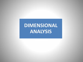
8. DIMENSIONS OF SOME COMMON PHYSICAL
QUANTITIES
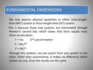
[x], Length – L
[m], Mass – M
[t], Time – T
[v], Velocity – LT-1
[a], Acceleration – LT-2
[F], Force – MLT-2
[Q], Discharge – L3T-1
[r], Mass Density – ML-3
[P], Pressure – ML-1T-2
[E], Energy – ML2T-2

9. BASIC CONCEPTS
 All theoretical equations that relate physical quantities must be
dimensionally homogeneous. That is, all the terms in an equation
must have the same dimensions. For example
 Q = A.V (homogeneous)
 L3T-1 = L3T-1
 We do, however sometimes use no homogeneous equation, the
best known example in fluid mechanics being the Manning
equation.


 Manning's equation is an empirical equation. Generally the use of
such equations is limited to specialized areas.

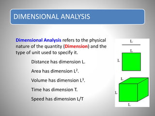
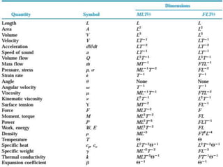
10. To illustrate the basic principles of dimensional analysis, let us
explore the equation for the speed V with which a pressure wave
travels through a fluid. We must visualize the physical problem to
consider physical factors probably influence the speed. Certainly
the compressibility Ev must be factor; also the density and the
kinematic viscosity of the fluid might be factors. The dimensions of
these quantities, written in square brackets are
V=[LT-1], Ev=[FL-2]=[ML-1T-2], r=[ML-3], ν=[L2T-1]
Here we converted the dimensions of Ev into the MLT system using
F=[MLT-2]. Clearly, adding or subtracting such quantities will not
produce dimensionally homogenous equations. We must therefore
multiply them in such a way that their dimensions balance. So let us
write
V=C Ev
a rb νd
Where C is a dimensionless constant, and let solve for the
exponents a, b, and d substituting the dimensions, we get

11. (LT-1)=(ML-1T-2)a (ML-3)b (L2T-1)d
To satisfy dimensional homogeneity, the exponents of each
dimension must be identical on both sides of this equation. Thus
For M: 0 = a + b
For L: 1 = -a -3b +2d
For T: -1 = -2a – d
Solving these three equations, we get
a=1/2, b=-1/2, d=0
So that V = C √(Ev/r)
This identifies basic form of the relationship, and it also determines
that the wave speed is not effected by the fluid’s kinematic
viscosity, ν.
Dimensional analysis along such lines was developed by Lord
Rayleigh.

12. METHODS FOR DIMENSIONAL ANALYSIS
Rayleigh’s Method
Buckingham’s ∏-method

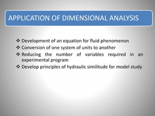
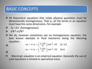
13. RAYLEIGH’S METHOD
Functional relationship between variables is
expressed in the form of an exponential relation
which must be dimensionally homogeneous
if “y” is a function of independent variables
x1,x2,x3,…..xn , then
In exponential form as
),.......,,( 321 nxxxxfy 
]),.......()(,)(,)[( 321
z
n
cba
xxxxy 

14. Procedure :
 Write MLT forms of the given data
 Write the same equation in exponential form
 Select suitable system of fundamental dimensions
 Substitute dimensions of the physical quantities
 Apply dimensional homogeneity
 Equate the powers and compute the values of the
exponents
 Substitute the values of exponents
 Simplify the expression
 Ideal up to three independent variables, can be used for
four.
RAYLEIGH’S METHOD

15. BUCKINGHAM’S ∏ METHOD
A more generalized method of dimension analysis developed by E.
Buckingham and others and is most popular now. This arranges the
variables into a lesser number of dimensionless groups of variables.
Because Buckingham used ∏ (pi) to represent the product of variables
in each groups, we call this method Buckingham pi theorem.
“If ‘n’ is the total number of variables in a dimensionally homogenous
equation containing ‘m’ fundamental dimensions, then they may be
grouped into (n-m) ∏ terms.
f(X1, X2, ……Xn) = 0
then the functional relationship will be written as
Ф (∏1 , ∏2 ,………….∏n-m) = 0
The final equation obtained is in the form of:
∏1= f (∏2,∏3,………….∏n-m) = 0
Suitable where n ≥ 4
Not applicable if (n-m) = 0

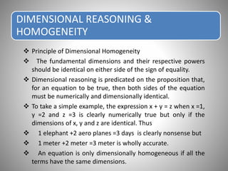
16. Procedure :
 List all physical variables and note ‘n’ and ‘m’.
 n = Total no. of variables
 m = No. of fundamental dimensions (That is, [M], [L], [T])
 Compute number of ∏-terms by (n-m)
 Write the equation in functional form
 Write equation in general form
 Select repeating variables. Must have all of the ‘m’
fundamental dimensions and should not form a ∏ among
themselves
 Solve each ∏-term for the unknown exponents by
dimensional homogeneity.
BUCKINGHAM’S ∏ METHOD

17. THANK YOU