SlideShare a Scribd company logo
1 of 76
Download to read offline
Rotations of Vectors
via Geometric Algebra:
Explanation, and Usage in Solving
Classic Geometric ”Construction” Problems
1
Geometric-Algebra Formulas
for Plane (2D) Geometry
The Geometric Product, and Relations Derived from It
For any two vectors a and b,
a · b = b · a
b ∧ a = −a ∧ b
ab = a · b + a ∧ b
ba = b · a + b ∧ a = a · b − a ∧ b
ab + ba = 2a · b
ab − ba = 2a ∧ b
ab = 2a · b + ba
ab = 2a ∧ b − ba
Definitions of Inner and Outer Products (Macdonald A. 2010 p. 101.)
The inner product
The inner product of a j-vector A and a k-vector B is
A · B = AB k−j. Note that if j>k, then the inner product doesn’t exist.
However, in such a case B · A = BA j−k does exist.
The outer product
The outer product of a j-vector A and a k-vector B is
A ∧ B = AB k+j.
Relations Involving the Outer Product and the Unit Bivector, i.
For any two vectors a and b,
ia = −ai
a ∧ b = [(ai) · b] i = − [a · (bi)] i = −b ∧ a
Equality of Multivectors
For any two multivectors M and N,
M = N if and only if for all k, M k = N k.
Formulas Derived from Projections of Vectors
and Equality of Multivectors
Any two vectors a and b can be written in the form of ”Fourier expansions”
with respect to a third vector, v:
a = (a · ˆv) ˆv + [a · (ˆvi)] ˆvi and b = (b · ˆv) ˆv + [b · (ˆvi)] ˆvi.
Using these expansions,
ab = {(a · ˆv) ˆv + [a · (ˆvi)] ˆvi} {(b · ˆv) ˆv + [b · (ˆvi)] ˆvi}
Equating the scalar parts of both sides of that equation,
2
a · b = [a · ˆv] [b · ˆv] + [a · (ˆvi)] [b · (ˆvi)], and
a ∧ b = {[a · ˆv] [b · (ˆvi)] − [a · (ˆvi)] [b · (ˆvi)]} i.
Also, a2
= [a · ˆv]
2
+ [a · (ˆvi)]
2
, and b2
= [b · ˆv]
2
+ [b · (ˆvi)]
2
.
Reflections of Vectors, Geometric Products, and Rotation operators
For any vector a, the product ˆvaˆv is the reflection of a with respect to the
direction ˆv.
For any two vectors a and b, ˆvabˆv = ba, and vabv = v2
ba.
Therefore, ˆveθiˆv = e−θi
, and veθi
v = v2
e−θi
.
3
The trouble with the very notion of ’application’ [of mathematics
to science, or of one branch of mathematics to another] is that it is
a one-way concept: we apply A to B. To counter this I have invented
the word ’interapplicability’. Mathematicians who work in these do-
mains more often speak of correspondence, which is a symmetric no-
tion. Although I began this discussion [of Descartes’s contributions]
in terms of application, we might better have spoken of Descartes
establishing a correspondence between arithmetic and geometry. I
once in conversation spoke of Descartes arithmetizing geometry; the
person with whom I was speaking, having in mind the way algebraic
problems of the day could now be solved geometrically, observed that
Descartes had geometrized algebra. Exactly so.1
1Hacking, Ian. 2014. Why is there Philosophy of Mathematics at All?. pp. 20-21.
Cambridge University Press, New York. I am grateful to “Lorena”, a student in philosophy
of Mathematics at La Universidad Nacional Aut´onoma de M´exico, for introducing me to this
book.
4
Rotations of Vectors via Geometric Algebra:
Explanation, and Usage in Solving Classic
Geometric ”Construction” Problems
Jim Smith
QueLaMateNoTeMate.webs.com
email: nitac14b@yahoo.com
February 11, 2016
Contents
1 Introduction 7
2 Important Facts about Tangents, Chords, and Angles 9
3 The Relationship between the Geometric Product and Rota-
tions 12
4 Using Exponential Expressions of Rotations to Solve Geometry
Problems 18
4.1 Problem 1 . . . . . . . . . . . . . . . . . . . . . . . . . . . . . . . 19
4.2 Problem 2 . . . . . . . . . . . . . . . . . . . . . . . . . . . . . . . 22
4.3 Problem 3 . . . . . . . . . . . . . . . . . . . . . . . . . . . . . . . 27
4.4 Problem 4 . . . . . . . . . . . . . . . . . . . . . . . . . . . . . . . 33
4.4.1 Solution Concept 1 . . . . . . . . . . . . . . . . . . . . . . 33
4.4.2 Solution Concept 2 . . . . . . . . . . . . . . . . . . . . . . 36
4.5 Problem 5 . . . . . . . . . . . . . . . . . . . . . . . . . . . . . . . 45
4.5.1 Solution Concept 1 . . . . . . . . . . . . . . . . . . . . . . 46
5
4.5.2 Solution Concept 2 . . . . . . . . . . . . . . . . . . . . . . 48
4.5.3 Solution Concept 3 . . . . . . . . . . . . . . . . . . . . . . 50
4.6 Problem 6 . . . . . . . . . . . . . . . . . . . . . . . . . . . . . . . 52
4.6.1 Solution Concept 1 . . . . . . . . . . . . . . . . . . . . . . 53
4.6.2 Solution Concept 2 . . . . . . . . . . . . . . . . . . . . . . 54
4.6.3 Solution Concept 3 . . . . . . . . . . . . . . . . . . . . . . 55
4.6.4 Solution Concept 4 . . . . . . . . . . . . . . . . . . . . . . 56
5 Literature Cited 58
6 Appendix A: Finding the Circumcenter Using the Inverse of a
Multivector 60
7 Appendix B: Useful Transformations of Products of Three and
Four vectors 69
7.1 Transforming Products of the Form ˆuvˆu . . . . . . . . . . . . . . 69
7.2 Useful Transformations of c2pt1p 2 . . . . . . . . . . . . . . . . 70
7.3 Transformations of Products of the Form uvwu . . . . . . . . . 73
8 Appendix C: Another Derivation of the Relationship between
Points of Tangency among Circles 74
6
1 Introduction
{Author’s note, 27 January 2016:
This document, in all of its versions, has been prepared for two very different
audiences: for my fellow students of GA, and for experts who are preparing ma-
terials for us, and need to know which GA concepts we understand and apply
readily, and which ones we do not. This new version should be useful to both
audiences. It presents a much easier way to find the circumcenter of a triangle
(pp. 22ff), but preserves the previous solution as Appendix A so that my ear-
lier oversights will be clear to readers. As a plus, that solution makes useful,
time-saving observations on inverses of multivectors, and on transformations of
vector expressions. }
{Author’s note, 27 January 2016:
I hope that the new material in this version will help students avoid forming
one of my own bad habits when using GA: the tendency to believe that GA can’t
possibly be as convenient as is claimed! That tendency can cause unnecessary
work by leading us to translate geometric products into quantities that are more
familiar, but much less efficient. In 4.2, we’ll learn time-saving maneuvers that
are available to us if we accept that GA’s theorems mean what they say.
A new section ( 2 ) provides background that will help us to formulate key aspects
of geometry problems in ways that can be manipulated via GA to find solutions.
The first three problems in this new version were added after I learned of the
solutions posted on line by Professor Ramon Gonz´alez Calvet, for the incenter
and circumcenter of a triangle. Professor Gonz´alez’s solutions do not use rota-
tions; the contrast between his insights and the ones used here is instructive.
A useful resource not mentioned in the previous version is ”Find tangents to
a circle from a point, using Geometric Algebra” (as GeoGebra worksheet, as
YouTube video). The present version solves that problem using rotations. }
{Introduction to the version of 31 December 2015:}
This document is part of a series of resources that I am preparing in support
of Professor David Hestenes’s goal of using Geometric Algebra (GA) to inte-
grate high-school algebra, geometry, trigonometry, and physics into a coherent
curriculum.
I will be grateful for any comments, suggestions, and corrections.
One important piece of advice before we start:
Don’t let yourself be intimidated by the equations that arise in
problems like these!
We’ll learn to recognize patterns (for example, products of four vectors that
represent a simple rotation) that will help us simplify complicated equations
readily. Also, I’ve presented more than one way to solve each problem. In addi-
7
tion to the way that appeared most reasonable and efficient, I’ve also included
at least one way ”sub-optimal” way, so that students can see that they needn’t
worry about having to find ”the way” to get the job done.
An additional benefit of presenting those sub-optimal ways (some of which,
like 4.5.2 border on the absurd) is that they help demonstrate the coherence
and flexibility of GA’s capacities for expressing and manipulating rotations.
Readers are encouraged to study the following GeoGebra worksheets and
videos before beginning:
”Answering Two Common Objections to Geometric Algebra”
As GeoGebra worksheet
As YouTube video.
”Geometric Algebra: Find unknown vector from two dot products”
As GeoGebra worksheet
As YouTube video
For an more-complete treatment of rotations in plane geometry, be sure to
read Hestenes D. 1999, pp. 78-92. His section on circles (pp. 87-89) is especially
relevant to the present document. Macdonald A. 2010 is invaluable in many
respects, and Gonz´alez Calvet R. 2001, Treatise of Plane Geometry through
Geometric Algebra is a must-read.
What we’ll see in this document ...
• Rotations of vectors as a natural development of the inner, outer, and
geometric products
• How ”construction” problems of classical geometry can be formulated in
terms of rotations and dilations of vectors, then solved by
– recognizing the geometric content of equations that arise; and
– making use of postulates about equality of multivectors.
• How Professor Alan Macdonald’s definitions of the inner and outer prod-
ucts simplify the solution process.
• How to simplify complicated products by
– using basic identities; and
– recognizing products that represent rotations and reflections
• Most importantly: That all this stuff about angles, exponents, and
geometric products really is coherent, and terms like eθi
really do follow
the rules of exponents.
The author may be contacted at QueLaMateNoTeMate.webs.com.
8
2 Important Facts about Tangents, Chords, and
Angles
This information provided in this section will help us to formulate problems in
symbolic terms that can be manipulated via GA to find solutions. Some of the
relationships listed here are provided for completeness, and are not used in this
document.
1. The mediatrix (perpendicular bisector) of a chord of a circle passes through
the circle’s center.
This important result from classical geometry can be proven simply via
GA. Using the circle’s center as the origin, the chord AB becomes the
vector a − b, and the vector from the center of the circle to the midpoint
of AB is
1
2
(a + b) .
The symbol ” ” is an
alternative to ”QED”: both are
used to show that the proof has
been completed.
According to the postulates of GA, two vectors are perpendicular if and
only if their dot product is zero, so let’s find (a − b)·(a + b). The vectors
a and b are radii of the same circle, so |a| = |b|. Therefore,
(a − b) · (a + b) = a · a − a · b − b · a + b · b
= a2
− b2
= 0.
This result shows that the line that passes through the circle’s center and
the chord’s midpoint is perpendicular to the chord. Therefore, that line
is the chord’s mediatrix.
9
2. Two consequences of the perpendicularity between any chord and the
radius drawn to its midpoint are
(a) that the line connecting the centers of two intersecting circles is per-
pendicular to their common chord;
and
(b) that the line line connecting the centers of two tangent circles passes
through the point of tangency.
3. The two tangents drawn to a circle from an external point are of equal
length: NS = NF.
4. A tangent to a circle is perpendicular to the line that passes through the
circle’s center and the point of tangency.
10
For a GA proof of this relationship, see ”Find tangents to a circle from
a point, using Geometric Algebra”(as GeoGebra worksheet, as YouTube
video).
5. An angle inscribed in a circle is equal to half the central angle that sub-
tends the same arc. For example, all of the purple angles—including the
angle formed by the segment BA and the ray
−→
R subtend the same arc
(ABD). For details, see Hestenes D. 1999, p. 89. Therefore, all are equal
to each other, and measure
1
2
∠DCA.
A corollary is that any angle inscribed in a semicircle is a right angle:
6. The measure of an angle whose vertex lies outside a circle is equal to half
the difference between the measures of the central angles that subtend
the arcs cut by the rays that form the angle’s sides. For example, θ =
1
2
(α − β).
11
(Note that GA’s sign convention for angles is that counter-clockwise ro-
tations are positive.) A special case of this relationship is the angle
between the tangents drawn to a circle from an external point: θ =
1
2
[(2π − β) − β] = π − β.
7. The measure of an angle whose vertex lies inside a circle is equal to half
the sum the measures of the central angles that subtend the arcs cut by
the lines that form the angle’s sides. For example, θ =
1
2
(α + β).
3 The Relationship between the Geometric Prod-
uct and Rotations
Let’s begin by reviewing a variation on a sequence of operations that we saw in
the worksheet and video, ”Answering Two Common Objections to Geometric
Algebra”:
12
https://www.youtube.com/watch?v=oB0DZiF86Ns
http://tube.geogebra.org/material/simple/id/1565271.
Given any two vectors a and b, we can express b as the vector sum of
its projections upon a and ai, where i is the unit bivector of the plane that
contains a and b. (Please recall that ai is the 90◦
counter-clockwise rotation
of a.)
b = Pa (b) + Pai (b)
= (b · ˆa) ˆa + b · ˆai ˆai
=
|b|
|a|
a ˆb · ˆa + ˆb · ˆai ˆi .
Looking now at our diagram, we can see that ˆb · ˆa = cos θ and ˆb · ˆai =
sin θ.
Therefore, we can write that last result as
b =
|b|
|a|
a (cos θ + sin θi) ,
one geometrical interpretation of which is that b is obtained by rotating a
counterclockwise through the angle θ, and dilating it by the factor |b|/|a|. (Or
by dilating, then rotating; the operations commute.)
Now, we write cos θ + sin θi in exponential form, as eθi
, to obtain
b =
|b|
|a|
aeθi
.
Before we proceed, we should do a few trial calculations to assure ourselves
that the preceding formulas work, and that we understand them. For example,
we know that if we rotate the vector a clockwise by 90◦
(π/2 radians), then
dilate it by a factor of 2, we obtain the vector 2ai. Let’s see whether that’s the
13
result that we obtain from our formulas:
2
1
a cos
π
2
+ sin
π
2
i = 2a (0 + 1i) = 2ai.
We also know that if we rotate a through the angle θ, then rotate the
resulting vector through the angle φ, the result should be the vector a rotated
through the angle θ + φ. Is that what the formulas tell us? Using the symbol
a to represent the vector that’s obtained by the rotation through θ, we have
a = a (cos θ + sin θi) .
The rotation of that vector (a ) through the angle φ is then
a = a (cos φ + sin φi)
= [a (cos θ + sin θi)]
a
(cos φ + sin φi)
= a cos θ cos φ + sin θ sin φi2
+ (cos θ sin φ + sin θ cos φ) i
= a [(cos θ cos φ − sin θ sin φ) + (cos θ sin φ + sin θ cos φ) i]
= a [cos (θ + φ) + sin (θ + φ) i] ,
which is a rotated through the angle θ + φ. We could have obtained that same
result using the exponential form:
a = aeθi
a
eφi
= ae(θ+φ)i
= a [cos (θ + φ) + sin (θ + φ) i] .
These encouraging results should help us see that the formulas that we’ve
developed thus far really do provide convenient ways of expressing and manip-
ulating rotations of vectors symbolically. But now, we’ll do something that at
first sight seems pointless, even if correct. Starting from our result b =
|b|
|a|
aeθi
,
where θ is the angle from a to b, we can see that
ab = a
|b|
|a|
aeθi
=
|b|
|a|
a2
eθi
=
|b|
|a|
|a|
2
eθi
= |a| |b| eθi
.
So, the geometric product ab is equal to |a| |b| eθi
. This result, too, deserves
some discussion before we continue. Let’s start by considering what happens to
14
some third vector v, coplanar with a and b, when we right-multiply that vector
by ab :
v (ab) = v |a| |b| eθi
= |a| |b| veθi
,
More generally, the product of
any two vectors evaluates to the
sum of a scalar and a bivector,
so in plane (2-D) geometry, the
product of any even number of
vectors must also evaluate to
the sum of a scalar and a
bivector, while the product of
any odd number of vectors
evaluates to a vector. This fact
will be important to us later.
For example, see the margin
note ”A word about what we’re
working toward here” (p. 37 ).
meaning that when right-multiplied by ab, the vector v is dilated by the scalar
factor |a| |b|, then rotated through the angle θ. Hildebrand and Oldenburg
2015 were referring to this property of the geometric property when they said
that geometric products are used for handling transformations. We should
also note that both |b|
|a|
eθi
and |a| |b| eθi
have the form of the product of (1) a
scalar dilation factor; and (2) an operator that rotates by an angle equal to that
between a and b. Incidentally, this result also shows that the product of any
three coplanar vectors is a vector. We’ll make use of that important fact later.
Of course we should also note that because ab = |a| |b| eθi
,
ab
|a| |b|
= eθi
.
When we need to rotate vectors to solve ”construction” problems later in this
video, we’ll use that equivalence as a convenient way to obtain an expression
for eθi
.
Those of you who’ve studied rotations may be be objecting that the way
to rotate a vector v through the angle θ is to multiply v on the left by e
−
θ
2
i
,
and on the right by e
θ
2
i
:
e
−
θ
2
i
ve
θ
2
i
= v, rotated ccw by θ.
This is a very brief —and not
entirely satisfactory —
explanation of what i represents
in 3-D rotations. For details,
see Macdonald 2010, pp. 89-91
and 125-127.
That’s true: it’s the form used in 3-D (and higher), with i being the unit
bivector for the plane of rotation. But in 2-D, e
−
θ
2
i
ve
θ
2
i
reduces to eθi
, as we’ll
now see:
e
−
θ
2
i
ve
θ
2
i
= cos −
θ
2
+ sin −
θ
2
i v cos
θ
2
+ sin
θ
2
i
= cos
θ
2
− sin
θ
2
i v cos
θ
2
+ sin
θ
2
i
= cos
θ
2
v − sin
θ
2
iv cos
θ
2
+ sin
θ
2
i
=

cos
θ
2
v + sin
θ
2
vi
=−iv

 cos
θ
2
+ sin
θ
2
i
= v cos
θ
2
+ sin
θ
2
i cos
θ
2
+ sin
θ
2
i
= ve
θ
2
i
e
θ
2
i
= ve
θ
2
i +
θ
2
i
= veθi
.
15
Before we leave the subject of rotations, we should treat the square root of
a rotation operator, such as the square root of the operator eαi
that rotates ˆu
into ˆv in the following figure.
There are times when we might wish to express the square root of that
operator in terms of ˆu and ˆv. For example, knowing that the central angle
formed by vectors a and b in the following figure is 2θ (page 11),
how could we express the operator that rotates b−x into a−x? That operator
involves a dilation as well as a rotation (except when |b − x| = |a − x|), so let’s
see first how we’d express the pure rotation eθi
in terms of ˆa and ˆb.
Let’s address that question by adding a few elements to our diagram in
which the operator eαi
rotated ˆu into ˆv.
16
Note how the familiar scalar
identity (pm
)n
≡ pmn
applies to
rotation operators as well:
√
eαi = eαi
1
2
= e
1
2
(αi)
= e
α
2
i
.
We see that the unit vector that bisects α is
(ˆu − ˆv) i
2 (1 − ˆu · ˆv)
. Two rotations
through the angle α/2 produce a rotation through α, so
√
eαi = e
α
2
i
= either of ˆu
(ˆu − ˆv) i
2 (1 − ˆu · ˆv)
and
(ˆu − ˆv) i
2 (1 − ˆu · ˆv)
ˆv,
both of which reduce to
e
α
2
i
=
i − ˆuˆvi
2 (1 − ˆu · ˆv)
.
Therefore, in the case of our diagram with the circle that passes through
the points a. b, and x,
we multiply the rotation operator e
α
2
i
by the dilation factor
|a − x|
|b − x|
, and find
17
that
a − x =
|a − x|
|b − x|
e
α
2
i
=
|a − x|
|b − x|




i − ˆbˆai
2 1 − ˆb · ˆa



 .
Now that we know how to find the square root of an operator that produces
a pure rotation, how can we find the square root of an operator of the form λeθi
(with scalar λ), which combines a dilation and a rotation? The exponents in
rotation operators obey all of the usual rules about exponents, so
√
λeθi =
√
λ
√
eθi
=
√
λe
θ
2
i
.
4 Using Exponential Expressions of Rotations
to Solve Geometry Problems
In this section, we’ll see that GA’s ability to manipulate rotations algebraically
enables us to solve a given problem in many different ways. We’ll make extensive
use of our results b = |b|
|a|
aeθi
, ab = |a| |b| eθi
, and v (ab) = v |a| |b| eθi
.
One important piece of advice before we start:
Don’t let yourself be intimidated by the equations
that arise in problems like these!
We’ll learn to recognize patterns (for example, products of four vectors that
represent a simple rotation) that will help us simplify complicated equations
readily.
18
4.1 Problem 1
Derive equations for the tangents to a circle from a point outside it.
Identifying Potentially Useful Elements of the Problem We’ll begin by
identifying elements of the problem that might be sufficient to provide sufficient
information for constructing one of the two tangents. The point t is a point
of tangency. In deriving our solution, we’ll used the same symbol —that is, t
—to denote both the point of tangency and the vector to that point from the
external point p. We’ll rely upon context to tell the reader whether t is being
used to refer to the point, or to the vector.
We can solve the problem if we can identify either of the angles θ and α,
or either of the vectors t and ˆt. What elements of the problem might help us
identify θ, α, t, and ˆt , and how are all of those quantities related?
|t − c| = r.
Firstly, because ptc is a right triangle, t2
= c2
− r2
. From Section 2 , we
find that θ =
1
2
[(π − α) − α] = π
2
− α. Therefore, θ + α =
π
2
. Finally, eθi
= ˆcˆt,
and eαi
=
t − c
|t − c|
(−ˆc) =
(c − t) ˆc
r
.
Formulating a Strategy Now, let’s combine that information in a way that
might lead us to a a solution. A reasonable way to begin is by noting that
19
because θ + α = π
2
, we can write
e(θ+α)i
= e
π
2
i
,
eθi
eαi
= i,
ˆcˆt
(c − t) ˆc
r
= i.
To put that result in a more-convenient form, we’ll multiply both sides by
c2
r |t| (which is also |c|
2
r |t|) to obtain
ct (c − t) c = c2
r |t| i.
The symbol ”≡” is used to
communicate that the
quantities uvwu and u2
wv are
”equivalent”, or ”identical”:
they’re equal for any three
coplanar vectors, not just for
some three particular vectors of
interest.
As shown in the Appendix (7.3) , for any three coplanar vectors u, v and ,
w, uvwu ≡ u2
wv. (Note the reversal of the order of v and w.) That identity
enables us to make the following simplifications:
ct (c − t) c = c2
r |t| i,
c [t (c − t)] c = c2
r |t| i,
c2
ct − t2
= c2
r |t| i,
ct − t2
= r |t| i.
Solving the Equation That last result is quite concise, but is it useful to
us? Yes: to obtain t from ct, we just left-multiply by c−1
. The other quantities
in the result that we just obtained are already known to us: t2
= c2
− r2
, so
|t| =
√
c2 − r2. The rest is straightforward:
ct − t2
= r |t| i,
ct = c2
− r2
+ r c2 − r2 i,
c−1
ct =
c
c2
=c−1
c2
− r2
+ r c2 − r2 i ,
t = c2
− r2 c
c2
+ r c2 − r2
c
c2
i,
= 1 −
r
|c|
2
c +

 r
|c|
1 −
r
|c|
2

 ci.
We’ve now identified one of the points of tangency. Finding the other (t2) turns
out to be easier.
20
Remember: ˆcˆc = 1, and for any
vector v, vˆv = ˆvv = |v|.
In this case, eθi
= ˆt2ˆc, and eαi
= (−ˆc)
t2 − c
r
=
ˆc (c − t2)
r
. Using those
expressions in our equation eθi
eαi
= i,
ˆt2ˆc
ˆc (c − t2)
r
= i,
ˆt2ˆcˆc (c − t2)
r
= i
ˆt2c − ˆt2t2 = ri,
t2c − t2t2 = r |t2| i,
t2c − t2
2 = r |t2| i,
t2c = t2
2 + r |t2| i,
∴ t2c = c2
− r2
+ r c2 − r2 i.
Comparing that equation to the analogous one that we obtained when
finding t,
ct = c2
− r2
+ r
√
c2 − r2 i,
Right-multiplying by c−1
, rather
than left-multiplying, has
inverted the sign of the ci term.
we see the right-hand sides are identical, but the order of the multiplication on
the left-hand side is inverted. To solve for t, we left-multiplied by c−1
, but we’ll
right-multiply by c−1
to solve for t2. What difference will that make? Let’s
see. . .
t2 = c2
− r2
+ r c2 − r2 i
c
c2
=c−1
= 1 −
r
|c|
2
c +

 r
|c|
1 −
r
|c|
2

 ic,
= 1 −
r
|c|
2
c +

 r
|c|
1 −
r
|c|
2

 (−ci)
=ci
,
= 1 −
r
|c|
2
c −

 r
|c|
1 −
r
|c|
2

 ci.
21
As a contrast that might prove useful, this problem is solved without using
rotations in ”Find tangents to a circle from a point, using Geometric Algebra”
(as GeoGebra worksheet, as YouTube video).
4.2 Problem 2
Derive an equation for the position of the circumcenter of a triangle with respect
to one of its vertices.
Identifying Potentially Useful Elements of the Problem This problem
can be solved in several different ways. For example, because the mediatrix
of any chord in a circle passes through the circle’s center (1 ), we can find the
circumcenter of our triangle by finding the point at which the mediatrices of
any two sides of the triangle intersect. We can also find the circumcenter via
simple trigonometry.
However, we wish to solve this problem by using rotations, so let’s begin by
asking, ”Is the circumcenter involved in the rotation of any identifiable vectors?”
As soon as we add the circumcenter to our previous diagram, and draw vectors
from the circumcenter to any two of the given triangle’s vertices,
22
Two methods of solving
problems via rotations:
• Equate two expressions
for the same angle (in
this case, α); and
• Write one vector as a
”rotation + dilation” of
the other. In this case,
c − q is a pure rotation
of b − q because both are
radii of the same circle.
Quite often, the equation
obtained via one of these
methods is much easier to solve
than that obtained via the
other.
we can see that the required circle converts the given triangle into ”three in-
scribed angles” (5). Therefore, we can choose any of the triangle’s vertices the
origin (we’ve chosen a), and write α = 2θ, from which eθi
eθi
= e2θi
.
Formulating a Strategy One strategy is to express the equality of angles
that we’ve just identified in terms of products of vectors, in order to obtain an
equation involving q:
eαi
= e2θi
eαi
= eθi
eθi
b − q
|b − q|
c − q
|c − q|
= ˆbˆc ˆbˆc .
Then, we’d expand both sides of the equation that we’ve just obtained, after
which we’d use other manipulations to identify q.
We’ll use that strategy in later problems, but before we dive into it here,
we should also note that c − q is a pure rotation of b − q because both are radii
of the same circle:
[b − q] eαi
= c − q
[b − q] eθi
eθi
= c − q
[b − q] ˆbˆc ˆbˆc = c − q,
b ˆbˆc ˆbˆc = bˆb ˆcˆbˆc
= |b| ˆcˆbˆc
= ˆc |b| ˆb ˆc
= ˆcbˆc.
from which
b ˆbˆc ˆbˆc − q ˆbˆc ˆbˆc = c − q,
q − q ˆbˆc ˆbˆc = c − b ˆbˆc ˆbˆc ,
q 1 − ˆbˆcˆbˆc = c − b ˆbˆc ˆbˆc
q 1 − ˆbˆcˆbˆc = c − ˆcbˆc.
23
Is that result helpful? Yes, because 1− ˆbˆcˆbˆc has a multiplicative inverse in
GA. Therefore, we can write the following in a purely formal way, then identify
what that inverse is, precisely:
q 1 − ˆbˆcˆbˆc 1 − ˆbˆcˆbˆc
−1
= (c − ˆcbˆc) 1 − ˆbˆcˆbˆc
−1
∴ q = (c − ˆcbˆc) 1 − ˆbˆcˆbˆc
−1
.
Appendix A (p. 60) solves for q
in this way. Although it’s more
complicated than the ways that
we’ll see here shortly, it’s
recommended (along with the
comments thereon) for its
time-saving pointers regarding
inverses of multivectors, and for
its observations on geometric
interpretation of results and
transformations of vectors.
However, is there an even-easier way? Let’s add a few more elements to
our diagram, then examine it again:
We see now that a rotation through our angle θ, in combination with a dilation
by the scalar factor
|d − q|
|b − q|
, will transform the vector b − q into d − q:
d − q =
|d − q|
|b − q|
(b − q) eθi
=
|d − q|
|b − q|
(b − q) ˆbˆc.
The next few paragraphs
indicate how we’d use ordinary
trigonometry to identify the
position of the incenter with
respect to the midpoint of
segment bc. Note also that
|b − c|
2
= |b − d|
= |b − q| ˆbi · ˆc
∴ |b − q| =
|b − c|
2 ˆbi · ˆc
.
Determining the value of
|d − q|
|b − q|
is easy enough: d − q is the projection of b − q
upon (b − c) i, so
|d − q| = |b − q| cos θ
= |b − q| ˆb · ˆc;
∴
|d − q|
|b − q|
= ˆb · ˆc.
Putting these observations and results together, our equation
d − q =
|d − q|
|b − q|
(b − q) ˆbˆc
24
becomes
d − q = ˆb · ˆc (b − q) ˆbˆc.
To solve that equation for q, we rearrange it as
q ˆb · ˆc ˆbˆc − 1 = ˆb · ˆc ˆbˆc − d,
then right-multiply both sides by ˆb · ˆc ˆbˆc − 1
−1
.
That task promises to be somewhat easier than finding q via the equation
that we obtained previously, which was
q = (c − ˆcbˆc) 1 − ˆbˆcˆbˆc
−1
.
Still, we can do even better. Let’s recall the first strategy that we identified for
finding q: that of writing the rotation operator e2θi
as the product of the unit
vector in the direction b−q and the unit vector in the direction c−q. Combining
that idea with the experience we’ve gained subsequently from formulating two
alternative strategies, we can see potential benefit in writing
The unit vector in the direction (b − c) i is the rotation, through the angle
θ, of the unit vector in the direction b − q.
That is,
(b − c) i
|b − c|
=
b − q
|b − q|
eθi
From our previous work, we can
derive that
|b − q|
|b − c|
=
1
2 ˆbi · ˆc
.
from which
|b − q|
|b − c|
(b − c) i = (b − q) ˆbˆc, and
qˆbˆc = bˆbˆc −

 (b − c) i
2 ˆbi · ˆc


= |b| ˆc −

 (b − c) i
2 ˆbi · ˆc

.
That equation is the one that we shall now solve.
Solving the Equation In the equation
qˆbˆc = |b| ˆc −

 (b − c) i
2 ˆbi · ˆc

,
25
q is right-multiplied by ˆbˆc . We can undo those operations by right-multiplying
by ˆcˆb, which of course happens to be ˆbˆc
−1
:
qˆbˆc ˆcˆb = |b| ˆc −

 (b − c) i
2 ˆbi · ˆc

 ˆcˆb
q = |b| ˆcˆcˆb −

(b − c) ˆicˆb
2 ˆbi · ˆc


= b +

cˆcˆb − bˆcˆb
2 ˆbi · ˆc

i
= b +


|c| ˆb − b 2ˆc · ˆb − ˆbˆc
2 ˆbi · ˆc

i
= b +


|c| ˆb + |b| ˆc − 2 ˆb · ˆc b
2 ˆbi · ˆc

i
Appendix A (p. 60) discusses in
detail many aspects of finding
inverses of multivectors. One
quick way to see that ˆbˆc
−1
is
ˆcˆb is by noting that ˆbˆc = eθi
,
the multiplicative inverse of
which is e−θi
, which in turn, as
we can deduce from our
diagrams, is ˆcˆb.
This answer is satisfactory for computing q, but we can transform it into a
version that’s more useful and informative.
Interpreting the Solution, and Transforming It into a More-Useful
Form Readers are encouraged to review the extensive treatment that this
subject is given in Appendix A (p. 60), for the version of the solution obtained
by solving the equation
q = (c − ˆcbˆc) 1 − ˆbˆcˆbˆc
−1
.
Here, we’ll transform the solution that we just obtained into a form that shows
that q lies along the mediatrix of segment bc. We begin the transformation by
going back a few steps to
q = b +

cˆcˆb − bˆcˆb
2 ˆbi · ˆc

i,
26
then continuing
q = b +


cˆcˆb − b 2ˆb · ˆc − ˆbˆc
2 ˆbi · ˆc

i
= b +


cˆcˆb + bˆbˆc − 2 ˆb · ˆc b
2 ˆbi · ˆc

i
= b +


c ˆc · ˆb + ˆc ∧ ˆb + b ˆb · ˆc + ˆb ∧ ˆc − 2 ˆb · ˆc b
2 ˆbi · ˆc

i
= b +


(c − b) ˆb · ˆc + (b − c) ˆb ∧ ˆc
2 ˆbi · ˆc

i
= b +


(c − b) ˆb · ˆc + (b − c) ˆbi · ˆc i
2 ˆbi · ˆc

i
= b +


ˆb · ˆc
ˆbi · ˆc

 c − b
2
i +
c − b
2
=
b + c
2
+
ˆb · ˆc
ˆb · (ˆci)
b − c
2
i .
The geometric significance of that version is shown in the following figure:
As we knew from the classical solution and from trigonometry, q lies along the
mediatrix of segment bc.
4.3 Problem 3
Derive an equation for the position of the incenter of a triangle with respect to
one of its vertices.
27
Identifying Potentially Useful Elements of the Problem Although the
problem is posed as one of finding the incenter, we can see that each of the
triangle’s vertices is a point from which tangents are drawn to the required
circle. Thus, we have three cases of Problem 1 (4.1). So, let’s choose one of the
vertices as the origin, then identify elements that might be useful.
One key fact is that from Problem 1, we know that the incenter must lie
along the bisector of the angle formed by the tangents drawn to the circle. Thus
the incenter lies along the direction
ˆb + ˆc
2
. A second is that the radii from the
incenter to the points of tangency are perpendicular to the triangle’s sides. A
third is that the lengths of the tangents from each vertex are equal. From the
latter, we can deduce that the length of the segment cb is equal to the sum of
the lengths of segments cg and bf.
We can also see several rotations that we might be able to formulate via
GA and use to find the answer, so let’s add a few more elements to our figure
so that we can treat those rotations more precisely.
28
Although we drew this diagram in order to examine rotations, we can see that
it also helps us refine our initial observations about lengths of segments. Why
not do so now, before moving on to the rotations?
We noted that the sides of the triangle are perpendicular to the radii drawn
from the incenter, so we know that vector f is q’s projection upon ˆb:
f = q · ˆb ˆb.
Because the two tangents drawn to a circle from a given point are equal in
length, we know that |g| = |f|. Therefore,
g = q · ˆb ˆc.
Our initial observation that the length of segment bc is the sum of the
lengths of segments cg and bf can also be translated into a ”GA-friendly”
vector equation:
|c − b| = |g − c| + |f − b|
= |c| − |g| + |b| − |f|
= |c| − q · ˆb + |b| − q · ˆb.
Therefore,
q · ˆb =
|b| + |c| − |c − b|
2
.
That result is sure to be important; we could solve for q immediately if
we knew the geometric product qˆb, and all we need to do in order to form
that product is to determine the outer product q ∧ ˆb. That outer product will
probably arise somewhere in the expressions for rotations that we intend to
examine, so let’s turn to those now.
29
One of those rotations is that of vector f through the angle θ to give vector
g:
g = feθi
, with eθi
= ˆbˆc.
A more-exotic example is illustrated by the following diagram.
We express the vector h in two ways: as q plus the rotation of f − q through
the angle β,
h = q + (f − q) eβi
.
and as the vector b plus the rotation of f − b through the angle ψ:
h = b + (f − b) eψi
.
30
The rotation operator eψi
can be written as the geometric product −ˆb
c − b
|c − b|
=
|b| − ˆbc
|c − b|
. To derive an expression for β, we use the theorem about the measure
of an angle drawn from a point exterior to a circle (p. 11). The angles β and
δ are shown as negative (clockwise) angles in our diagram, so β + δ = −2π.
Therefore,
ψ =
1
2

β − (−2π − β)
=δ

 ,
= β + π,
from which β = ψ − π (which is clearly a negative angle).
These observations appear to have provided enough information —and in
”GA-friendly form”—to solve the problem, so let’s formulate a strategy.
Formulating a Strategy Our observations have suggested two strategies:
1. Identify q from the known value of q · ˆb and from the value of q · ˆb, which
is still unknown, but which we should be able to determine by analyzing
rotations; and
2. Although the solution via the
second strategy is not presented
in this document, that strategy
does work. Equating the two
expressions for h gives
q + (f − q) eβi
= b + (f − b) eψi
,
q + (q − f) eψi
= b + (f − b) eψi
,
and
q (1 + b) eψi
= b 1 − eψi
+ 2feψi
.
From there, we’d right-multiply
both sides by 1 + eψi −1
to
solve for q . See Appendix A (p.
60) for the method.
Equate the two expressions that we obtained for the vector h:
h = b + (f − b) eψi
.
and
h = q + (f − q) eβi
.
with f = q · ˆb ˆb =
|b| + |c| − |c − b|
2
ˆb, and
eβi
= e(ψ−π)i
= eψi
e(−π)i
=−1
= −eψi
=
ˆbc − |b|
|c − b|
.
An important piece of
information that neither of our
strategies uses.
We’ll use the first strategy because it appears to be simpler. However,
this is a good moment to note that neither of the strategies makes use of an
important observation that we made earlier: the point q lies along the direction
ˆb + ˆc
2
. We can express that observation in terms such as
q ∧ ˆb + ˆc = 0, and q ∧ ˆb + q ∧ ˆc = 0.
Let’s summarize the information that we’ve identified as relevant to the
strategy we’ve chosen:
31
q · ˆb =
|b| + |c| − |c − b|
2
q ∧ ˆb + ˆc = 0, or equivalently, q ∧ ˆb + q ∧ ˆc = 0.
Having formed q ∧ ˆb + ˆc so easily, and recognizing that we’d need to work a
bit to find q∧ˆc, we might ask now whether we’d be better off finding q· ˆb + ˆc ,
so that we can then find q from the geometric product q ˆb + ˆc . This moment
in our solution process is where our initial exploration of lengths of segments
pays off: we found that |g| = |f| = q · ˆb =
|b| + |c| − |c − b|
2
. That additional
information makes the route clear to us:
q · ˆb + ˆc = q · ˆb + q · ˆc = |b| + |c| − |c − b| ;
q ∧ ˆb + ˆc = 0;
∴ q ˆb + ˆc = q · ˆb + q · ˆc = |b| + |c| − |c − b| .
We’ll find q by solving that equation.
Solving the Equation Our equation is
q ˆb + ˆc = q · ˆb + q · ˆc = |b| + |c| − |c − b|,
which we solve via
q ˆb + ˆc ˆb + ˆc
−1
= [|b| + |c| − |c − b|] ˆb + ˆc
−1
q = [|b| + |c| − |c − b|]



ˆb + ˆc
ˆb + ˆc
2



= [|b| + |c| − |c − b|]
ˆb + ˆc
2 + 2ˆb · ˆc
=
|b| + |c| − |c − b|
1 + ˆb · ˆc
ˆb + ˆc
2
.
Interpreting the Solution The incenter lies along the bisector of the angle
formed by sides b and c, at a distance from point a equal to
|b| + |c| − |c − b|
1 + ˆb · ˆc
times the length of
ˆb + ˆc
2
.
Because the assumptions that we made about the vertex a apply to all three
vertices of any triangle, our solution is valid for all vertices of every triangle.
Therefore, the incenter is the point of intersection of the bisectors of the three
angles formed by the sides of the triangle. This result is the same as that
obtained via classical geometry.
32
4.4 Problem 4
Given two circles, and a point p on one of them, construct the circles that are
tangent to both of the given circles, with p being one of the points of tangency.
This problem has two solutions (i.e., the red and magenta circles). We’ll
find them in four ways, using two different concepts.
4.4.1 Solution Concept 1
In this first solution, we won’t think about the problem in terms of rotating
vectors; instead, we’ll use the expressions that we’ve developed as a means of
expressing angles between pairs of vectors in a convenient way. From there,
we’ll go on to solve for the vectors from the origin to the points of tangency
between the given circles and the ones that we’re asked to construct. Please
note that the solution presented here, although it uses the same ideas as the one
presented in ”Answering Two Common Objections to Geometric Algebra” (on
YouTube, on GeoGebraTube), is considerably ”cleaner” because we’re using
the starting point of the vectors t1 and t2 is used as the origin, rather than the
center of the circle on which p is located.
33
The angle between the directions of vectors t1 and p−t1 is θ, in the positive
(i.e., ccw) direction. Because the triangle pt1c2 is isosceles, the angle between
the directions of t1 −p and p−c2 is θ as well. Also, |t1| = r1, and |p − c2| = r2.
Therefore,
t1 (p − t1) = |t1| |p − t1| eθi
= r1 |p − t1| eθi
;
and
(t1 − p) (p − c2) = |t2| |p − c2| eθi
= r2 |p − t1| eθi
,
from which
(t1 − p) (p − c2) =
r2
r1
t1 (p − t1) .
Additional details on the
maneuvers needed here can be
found in Appendix C (page 74 )
and in ”Answering Two
Common Objections to
Geometric Algebra”:
On YouTube
On GeoGebraTube.
In those sources, you’ll also find
other ways to solve such
equations.
Expanding both sides, recognizing that t2
1 = r2
1, and rearranging, we obtain
t1
r2
r1
− 1 p + c2 = r1r2 + pc2 − p2
.
Now, we right-multiply both sides by the inverse of
r2
r1
− 1 p + c2 to
solve for t1. (Recall that the inverse of a vector v is v/ |v|
2
.) After rearranging
the right-hand side, we arrive at
t1 =
r2
2 − r1r2 + c2
2 −
r2
r1
− 1 p2
+ 2
r2
r1
− 1 p · c2 p + r1r2 −
r2
r1
p2
c2
r2
r1
− 1
2
p2 + c2
2 + 2
r2
r1
− 1 p · c2
.
To find t2, we recognize that the angles φ are equal.
34
Using the same ideas as in the solution for t1, we write
−t2 (p − t2) = |−t2| |p − t2| eφi
= r1 |p − t2| eφi
;
and
(t2 − p) (p − c2) = |t2| |p − c2| eφi
= r2 |p − t1| eφi
,
which leads to
t2
r2
r1
+ 1 p − c2 = r1r2 − pc2 + p2
,
and
t2 =
r2
2 + r1r2 + c2
2 +
r2
r1
+ 1 p2
− 2
r2
r1
+ 1 p · c2 p +
r2
r1
p2
− r1r2 c2
r2
r1
+ 1
2
p2 + c2
2 − 2
r2
r1
+ 1 p · c2
.
You’ve probably been thinking that the problem asks us to do more than
find t1 and t2: we’re required to identify (that is, to give equations for) the
tangent circles. So, now that we’ve found the points of tangency, how do we
proceed?
35
We can also express e
α
2
i
directly
in terms of the vectors c2 − p
and t2. See page 16 .
One possibility is given in Hestenes D. 1999, pp. 88-89. We’ll use the
magenta circle as our example. Knowing t2, we can determine the angle α.
Thus, we know that every point x on the magenta circle satisfies the condition
expressed by the equation
(p − x)
−1
(t2 − x) = δe
α
2
i
,
where δ is a scalar, −∞ < δ < ∞ . To each finite value of δ, there corresponds
a unique point x; the absolute value of δ increases without limit (”goes to
infinity”) as x approaches p.
4.4.2 Solution Concept 2
In our second Solution Concept, we makes life more difficult for ourselves—deliberately—in
order to demonstrate ideas that will prove helpful in more-difficult problems
later on. We begin by re-examining our figure, and noting from plane geome-
try, the angle between the vectors p − c3 and t1 − c3 is 2ψ.
36
Thus
t1 − c3 = (p − c3) e2ψi
.
To obtain an expression for eψi
, we can use either
[− (p − c2) i] (t1 − p)
|(−p − c2| i| |t1 − p|
or
(p − t1) t1i
|p − t1| |t1i|
.
We’ll opt for the latter, because it promises to be simpler to use. From the
preceding, we can see that we can obtain the vector t1 − c3 by rotating the
vector p − c3 counterclockwise through the angle ψ twice:
(p − c3) eψi
eψi
= t1 − c3.
A word about what we’re
working toward here: We’re
going to try to form an equation
in which one side is a product of
vectors, and the other is either a
pure scalar or a pure bivector.
Then, we’ll use postulates about
the equality of multivectors to
obtain an equation that we can
solve simply for t1.
That information doesn’t appear useful until we recognize that p − c3 =
−
r3
r2
(p − c2), and t1 − c3 = −
r3
r1
t1. Making these substitutions, and using the
expression that we chose for eψi
, the previous equation becomes
−
r3
r2
(p − c2)
=p−c3
(p − t1) t1i
|p − t1| |t1i|
(p − t1) t1i
|p − t1| |t1i|
= −
r3
r1
t1.
We can simplify that result, using |t1i| = r1, thereby finding that
(p − c2) (p − t1) t1i (p − t1) t1i = r1r2 |p − t1|
2
t1.
”Switching places of i’s and
vectors” is a common and
important maneuver that we’ll
use many times in this
document. You’ll learn to
simplify it quite soon: just
examine the term on which
you’re working, and count the
number of ”switches” that will
be needed to bring the i’s
together within that term to
make a ”-1”. That is, an ”i2
”.
If that number is even, then the
sign of the term inverts; if odd,
the sign remains unchanged. In
the present example, we made
two switches, so the sign
inverted.
Next, we eliminate the two factors i on the left-hand side by ”bringing
them together”. To do so, we just make a series of ”switches” of place between
one of the i’s and an adjacent vector. We use the identify iv ≡ −vi to keep
track of sign changes:
(p − c2) (p − t1) t1i (p − t1) t1i = r1r2 |p − t1|
2
t1
Repeating the previous equation
,
37
− (p − c2) (p − t1) t1 (p − t1) i
1st switch
t1i = r1r2 |p − t1|
2
t1,
(p − c2) (p − t1) t1 (p − t1) t1i
2nd
i = r1r2 |p − t1|
2
t1,
(p − c2) (p − t1) t1 (p − t1) t1i2
= r1r2 |p − t1|
2
t1,
(p − c2) (p − t1) t1 (p − t1) (−1) = r1r2 |p − t1|
2
t1,
(p − c2) (p − t1) t1 (p − t1) = −r1r2 |p − t1|
2
t1.
The key equation for Concept 2
Right-multiplying now by t1
−1
, we obtain the key equation for Concept 2:
(p − c2) (p − t1) t1 (p − t1) = −r1r2 |p − t1|
2
.
The right-hand side is a scalar. That result deserves several comments. The
first is that as we saw earlier, the geometric product of any three coplanar
vectors is another vector in the same plane. Therefore, the geometric product
of any four coplanar vectors is the sum of a scalar and a bivector, only. More to
the point, because (p − c2) (p − t1) t1 (p − t1) evaluates to a scalar, its bivector
part is zero:
(p − c2) (p − t1) t1 (p − t1) 2 = 0.
We’ll see, shortly, how to make use of that fact, but first let’s note an-
other important aspect of our key equation: it contains the sequence of factors
(p − t1) t1 (p − t1), which is of the form uvu. That’s noteworthy because for
any two vectors v and ˆu, the product ˆuvˆu is the reflection of v with respect
to ˆu. Hence, (p − t1) t1 (p − t1) is the reflection of t1 with respect to (p − t1),
and multiplied by the factor |p − t1|
2
. Based upon those observations, and upon
|p − c2| = r2 and t1 = r1, we can see that the equation
(p − c2) (p − t1) t1 (p − t1) = −r1r2 |p − t1|
2
tells us that (p − t1) t1 (p − t1) is equal to |p − t1|
2
t1 in magnitude, and is
parallel to p − c2, but opposite in direction.
Now that we’ve discussed some of the geometric significance of the equation
(p − c2) (p − t1) t1 (p − t1) = −r1r2 |p − t1|
2
,
we’ll solve that equation in three ways.
Concept 2, Solution Method 1 As noted above, the right-hand side of our
key equation (Page 38)
(p − c2) (p − t1) t1 (p − t1) = −r1r2 |p − t1|
2
Now we see why we wanted (p.
37) an equation in which one
side was either a pure scalar or
a pure bivector: The left-hand
side of our key equation is the
product of an even number of
vectors, so it must evaluate to a
multivector that’s the sum of a
scalar and a bivector. Because
the right-hand side is a pure
scalar, the bivector part of the
left-hand side must be zero.
is a scalar. Therefore,
(p − c2) (p − t1) t1 (p − t1) 2 = 0.
38
To use that fact, we’ll begin by expanding the left-hand side, then simpli-
fying. (Again, t2
1 = r2
1.)
(p − c2) (p − t1) t1 (p − t1) = ppt1p − ppt1t1 − pt1t1p + pt1t1t1 − c2pt1p
+c2pt1t1 + c2t1t1p − c2t1t1t1
= p2
t1p − 2r1
2
p2
+ r1
2
pt1 − c2pt1p + 2r1
2
c2p
−r1
2
c2t1.
Now, we need to identify the bivector part of the simplified expansion. The
bivector part of a sum of terms is the sum of the terms’ respective bivector
parts. (Note that r1
2
p2
is a scalar, so its bivector part is zero.) The only term
whose bivector part might cause us some trouble is c2pt1p. What is c2pt1p 2?
Several different ways of identifying it are presented in the Appendix (7.2).
The most straightforward way uses the identity that for any two vectors u and
v, uv ≡ 2u · v − vu. Therefore,
c2pt1p 2 = c2 (2p · t1 − t1p) p 2
= 2 (p · t1) c2p − p2
c2t1 2
= 2 (p · t1) c2 ∧ p − p2
c2 ∧ t1.
An important identity that’s
useful in solving equations that
arise when working with
rotations:
u ∧ v = [(ui) · v] i
= − [u · (vi)] i.
Using this expression, and our identity that for any two vectors u and v,
u ∧ v = [(ui) · v] i, we arrive at
(p − c2) (p − t1) t1 (p − t1) 2 = p2
− r1
2
c2 ∧ t1 − p2
− r1
2
p ∧ t1
−2 (p · t1) c2 ∧ p + 2r1
2
c2 ∧ p
= p2
− r1
2
[(c2i) · t1] i − p2
− r1
2
[(pi) · t1] i
−2 (p · t1) [(c2i) · p] i + 2r1
2
[(c2i) · p] i.
Now, we can make use of the fact that (p − c2) (p − t1) t1 (p − t1) 2 is
zero:
p2
− r1
2
[(c2i) · t1] i − p2
− r1
2
[(pi) · t1] i − 2 (p · t1) [(c2i) · p] i + 2r1
2
[(c2i) · p] i = 0,
which (after eliminating the factor i) we can rearrange as follows :
[2 (c2i) · p] p + p2
− r2
1 (pi − c2i)
W e ll call this vector ”z”
·t1 = 2r2
1 (c2i) · p.
Therefore,
t1 · ˆz =
2r2
1 (c2i) · p
|z|
.
That result is useful to us because we also know that t1 = (t1 · ˆz) ˆz +
[t1 · (ˆzi)] ˆzi, and t2
1 = r2
1. From those facts, we can show that
t1 · (ˆzi) = ± r2
1 − (t1 · ˆz)
2
.
39
But which root is correct: the positive, or the negative? To answer that ques-
tion, let’s attempt to identify the vector t2.
Looking again at our diagram, we find that
(p − c4) e2ϕi
= t2 − c4.
Proceeding now in the same way that we did to find t1,
−
r4
r2
(p − c2) eϕi
eϕi
=
r4
r1
t2
−
r4
r2
(p − c2)
(p − t2) (−t2i)
|p − t2| |−t2i|
=eϕi
(p − t2) (−t2i)
|(−t2i)| |−t2i|
=
r4
r1
t2
(p − c2) (p − t2) t2 (p − t2) t2 =
r2
r1
|p − t2|
2
|t2|
2
t2
Therefore,
(p − c2) (p − t2) t2 (p − t2) = r1r2 |p − t2|
2
.
Let’s compare that equation to the corresponding one that we obtained for
t1 (Page 38):
(p − c2) (p − t1) t1 (p − t1) = −r1r2 |p − t1|
2
The right-hand sides of the two equations have opposite algebraic signs. Those
signs, plus the fact that the right-hand sides are scalars, tell us that the vector
(p − t2) t2 (p − t2) is parallel to p − c2, while the vector (p − t1) t1 (p − t1) is
anti-parallel to it. Therefore, t1 and t2 are not the same vector.
Nevertheless, both of those vectors have the same length (= r1), and
both have the same projection upon z, as we can show by recognizing that
(p − c2) (p − t2) t2 (p − t2) 2 = 0, then proceeding as we did for t1. In this
way we arrive at
[2 (c2i) · p] p + p2
− r2
1 (pi − c2i)
T his is the same vector ”z” as for t1
·t2 = 2r2
1 (c2i) · p
=t1·z
,
40
∴ t2 · ˆz =
2r2
1 (c2i) · p
|z|
= t1 · ˆz.
Their components perpendicular to z are of equal length = r2
1 − (t1 · ˆz)
2
,
but are oppositely directed. (That’s why the vectors (p − t2) t1 (p − t1) and
(p − t2) t2 (p − t2) are oppositely directed.) Therefore, the solution obtained
by using the present method is
t =
2r2
1 (c2i) · p
|z|
ˆz ±



r1
2 −
2r2
1 (c2i) · p
|z|
2



ˆzi,
where
z = [2 (c2i) · p] p + p2
− r2
1 (pi − c2i) .
That form of the solution is satisfactory for computing t; if we wished,
we could transform it into another form by using ideas presented in the work-
sheet and video, ”Find unknown vector from two dot products” (as GeoGebra
worksheet , as YouTube video).
Concept 2, Solution Method 2 We’ll start from our key equation for this
concept (Page 38):
(p − c2) (p − t1) t1 (p − t1) = −r1r2 |p − t1|
2
.
In Solution Method 1 for this concept, we used the fact that the left-
hand side evaluates to a scalar, and thereby arrived at an equation for the dot
product t1 ·z. However, we made no use of the fact the left-hand side evaluates
to the specific scalar −r1r2 |p − t1|
2
. In the present Method, we’ll use that
information to find t1’s dot product with a second vector, which we’ll call ˆw1.
Knowing t1’s dot products with those two vectors, we’ll be able to find t1 using
methods developed in the worksheet and video, ”Find unknown vector from two
dot products” (As GeoGebra worksheet , As YouTube video).
41
From Method 1, we also know that (p − c2) (p − t1) t1 (p − t1) can be ex-
panded as
(p − c2) (p − t1) t1 (p − t1) = p2
t1p + r1
2
pt1 − r1
2
c2t1 + 2r1
2
c2p − 2r1
2
p2
− 2 (p · t1) c2p − p2
c2t1
=c2pt1p
.
Because |p − t1|
2
is (p − t1)
2
,
p2
t1p + r1
2
pt1 − r1
2
c2t1 + 2r1
2
c2p − 2r1
2
p2
− 2 (p · t1) c2p − p2
c2t1 = −r1r2 p2
− 2p · t1 + r1
2
=(p−t1)2
.
Equating the scalar parts of the two sides, and rearranging, we obtain
p2
+ r1
2
− 2 (r1r2 + c2 · p) p + p2
− r1
2
c2
W e ll call this w1.
·t1 = 2r1
2
p2
− c2 · p
−r1r2 p2
+ r1
2
.
Similarly, starting from
(p − c2) (p − t2) t2 (p − t2) = r1r2 |p − t2|
2
,
we find that
p2
+ r1
2
+ 2 (r1r2 − c2 · p) p + p2
− r1
2
c2
W e ll call this w2.
·t2 = 2r1
2
p2
− c2 · p
+r1r2 p2
+ r1
2
.
We now have a pair of ”dot-product” equations for each of the vectors t1
and t2:
z · t1 = 2r2
1 (c2i) · p,
w1 · t1 = 2r1
2
p2
− c2 · p − r1r2 p2
+ r1
2
.
z · t2 = 2r2
1 (c2i) · p,
w2 · t2 = 2r1
2
p2
− c2 · p + r1r2 p2
+ r1
2
.
In the worksheet and video ”Find unknown vector from two dot products”,
we learned that given the dot products of an unknown vector x with two known
vectors a and b, we can find x by writing it as a linear combination of a and b,
x = αa + βb,
from which we can then form the pair of linear equations
a · x = αa2
+ βa · b,
b · x = αa · b + βb2
.
42
Solving those equations for α and β, we obtain
α =
b2
a · x − (a · b) (b · x)
a2b2 − (a · b)
2 ,
β =
a2
b · x − (a · b) (a · x)
a2b2 − (a · b)
2 .
Making use of that solution, we find that
t1 = α1w1 + β1z,
where
α1 =
z2
w1 · t1 − (w1 · z) (z · t1)
w1
2z2 − (w1 · z)
2 ,
β =
w1
2
z · t1 − (w1 · z) (w1 · t1)
w1
2z2 − (w1 · z)
2 ,
w1 = p2
+ r1
2
− 2 (r1r2 + c2 · p) p + p2
− r1
2
c2,
w2 = p2
+ r1
2
+ 2 (r1r2 − c2 · p) p + p2
− r1
2
c2,
z = [2 (c2i) · p] p + p2
− r2
1 (pi − c2i),
w1 · t1 = 2r1
2
p2
− c2 · p − r1r2 p2
+ r1
2
,
w1 · t2 = 2r1
2
p2
− c2 · p + r1r2 p2
+ r1
2
,
z · t1 = z · t2 = 2r2
1 (c2i) · p.
Concept 2, Solution Method 3 Anyone who’s studied Geometric Alge-
bra—even casually—knows that the method usually prescribed for solving for
an unknown vector x in a given problem is to find x’s inner and outer products
with a known vector b, then proceed as follows:
x · b + x ∧ b = xb
x = (xb) b−1
Very antiseptic-looking! However, in this section, we’ll learn that x·b and x∧b
can take quite-complicated forms.
As we did in previous sections, we’ll start with our key equation:
(p − c2) (p − t1) t1 (p − t1) = −r1r2 |p − t1|
2
.
Again, we’ll expand the left-hand side. But this time, we’ll maintain p−c2
intact, as a single factor:
(p − c2) pt1p − 2r1
2
p + r1
2
t1
=(p−t1)t1(p−t1)
= −r1r2 |p − t1|
2
.
43
Examining the left-hand side, we see an interesting possibility: if we left-
multiply by (p − c2)
−1
, and right-multiply by p, we’ll obtain a sum of three
terms: a scalar, and two terms that are scalar multiples of geometric products
of p and t1. On the right-hand side, we’ll obtain a scalar multiple of the product
(p − c2) p:
(p − c2)
−1
(p − c2) pt1p − 2r1
2
p + r1
2
t1 p = (p − c2)
−1
−r1r2 |p − t1|
2
p
p2
pt1 + r1
2
t1p − 2r1
2
p2
= −
r1r2 |p − t1|
2
(p − c2)
2 (p − c2) p =
r1r2 |p − t1|
2
(p − c2)
2 c2p − p2
.
Now, we can develop expressions for t1 · p and t1 ∧ p. Equating the scalar
parts of both sides, and solving for t1 · p, we find that
t1 · p =
2r1
2
p2
(p − c2)
2
− r1r2 p2
+ r1
2
p2
− c2 · p
(p2 + r1
2) (p − c2)
2
− 2r1r2 (p2 − c2 · p)
.
Equating the bivector parts of both sides, we obtain
t1 ∧ p =
r1r2 p2
− 2t1 · p + r1
2
(p2 − r1
2) (p − c2)
2 [(pi) · c2] i
=p∧c2
.
Note that our expression for t1 ∧p contains the quantity t1 ·p. That’s fine,
because the expression for t1 ·p allows us to calculate the value of t1 ·p directly
from known quantities (r1, r2, p, and c2), after which we’d use that value to
calculate t1 ∧ p. If we wished, we could also do the work symbolically. That
is, we could substitute our expression for t1 · p into our expression for t1 ∧ p,
then do the algebra to obtain an expression for t1 ∧ p in terms of the known
quantities.
Having obtained these expressions for t1 · p and t1 ∧ p, how do we use
them to determine t1? This is where we need to understand the meaning of the
symbol ”+” in the ”antiseptic” version of the solution
t1 · p + t1 ∧ p = t1p
t1 = (t1p) p−1
.
We’ll see a brief explanation here; more details are given in the worksheet
and video ”Answering Two Common Objections to Geometric Algebra” (As
GeoGebra worksheet , As YouTube video). To solve for t1, starting from the
preceding equations, we write
t1 = (t1 · p + t1 ∧ p)
=t1p
p−1
= (t1 · p) p−1
+ (t1 ∧ p) p−1
=
t1 · p
p2
p +
t1 ∧ p
p2
p.
44
Every exterior product (including t1 ∧ p) is a scalar multiple of the unit
bivector i. Therefore, the second term on the right-hand side of the above
equation is a scalar multiple of ip, which is a vector. For that reason, the
second term is also a scalar multiple of −pi, where pi is the 90◦
counter-
clockwise rotation of p.
Therefore, the solution t1 =
t1 · p
p2
p +
t1 ∧ p
p2
p
expresses t1 as a linear combination of the vectors p and pi.
The analysis that we’ve just seen shows why we can view the operation
represented by the symbol ”+” in the definition x · b + x ∧ p = xb as a ”latent
vector addition” that becomes ”activated” when right-multiplied by a vector.
When multiplied by the vector b−1
, the result is x.
With that understanding, we can see how to put the product (t1 ∧ p) p−1
into a form that’s useful to us:
(t1 ∧ p) p−1
=
r1r2 p2
− 2t1 · p + r1
2
(p2 + r1
2) (p − c2)
2 [(pi) · c2] i
p
p2
=p−1
= −
r1r2 p2
− 2t1 · p + r1
2
p2 (p2 + r1
2) (p − c2)
2 [(pi) · c2] pi.
Therefore, the solution given by the present method is
t1 · p =



2r1
2
p2
(p − c2)
2
− r1r2 p2
+ r1
2
p2
− c2 · p
p2 (p2 + r1
2) (p − c2)
2
− 2r1r2 (p2 − c2 · p)



=(t1·p)/p2
p
−
r1r2 p2
− 2t1 · p + r1
2
p2 (p2 + r1
2) (p − c2)
2 [(pi) · c2] pi.
Again, this solution could be simplified algebraically. (We’ll omit the solu-
tion for t2.)
4.5 Problem 5
Given a circle and two points outside of it, identify the circles that are tangent
to the given one, and that pass through both of the given points.
45
We’ll see three ways to arrive at equations that can be solved for the points
of tangency by using Method 1 from Problem 4, Concept 2 (4.4.2).
4.5.1 Solution Concept 1
How would we proceed after
identifying the points of
tangency?
As is known from classical
geometry, we can construct a
circle if we know any three
points that lie on it. One of the
GA expressions of that truth is
that if c, d, and e are three
known points on a circle, then
every other point x on that
circle must satisfy the condition
expressed by the ”cross-ratio”
equation
(c − x)−1
(d − x)
(c − e)−1
(d − e)
= a scalar.
For details, see Hestenes D.
1999, p. 89.
In our case, for the circle that
contains t1, the known points
would be a, b, and t1, so one
version of the cross-ratio
equation for that circle would be
(a − x)−1
(b − x)
(a − t1)−1
(b − t1)
= ascalar.
Other versions can be obtained
by interchanging a, b, and t1.
This way is the simplest: we’ll begin by identifying the elements shown in
the following figure:
Now, we obtain two expressions for eθi
, and equate them to each other.
We’ll use the fact that |t1i| = |t1| = r:
(a − b) (t1 − b)
|a − b| |t1 − b|
=
(a − t1) t1i
|a − t1| |t1i|
Both sides are expressions for eθi
.
Next, we form an equation in which one side is a product of the vectors
that are involved, and the other side is either a scalar or a bivector:
46
(a − t1)
(a − b) (t1 − b)
|a − b| |t1 − b|
t1i = (a − t1)
(a − t1) t1i
|a − t1| |t1i|
t1i
(a − t1) (a − b) (t1 − b) t1i (−i) = |a − t1| |t1 − b| (a − t1) r (−i)
(a − t1) (a − b) (t1 − b) t1 = − |a − t1| |t1 − b| (a − t1) ri.
The right-hand side is a bivector, so (a − t1) (a − b) (t1 − b) t1 0 = 0. A
convenient way to expand (a − t1) (a − b) (t1 − b) t1 is via
a2
− ab − t1a + t1b t1
2
+ t1b ,
which works out to
b2
− r2
at1 − a2
− r2
bt1 + r2
a2
− b2
− r2
ab + t1abt1.
Therefore,
b2
− r2
at1 − a2
− r2
bt1 + r2
a2
− b2
− r2
ab + t1abt1 0 = 0.
The term t1abt1 is interesting. At the beginning of 4.4.2, we saw that the
product ˆuvˆu evaluates to a vector: specifically, the reflection of v with respect
to ˆu. Similarly, the product ˆuvwˆu is the reflection of the geometric product
vw. But let’s see exactly why that is, and what it means. We’ll discover that
the scalar part of vw: is unaffected by the reflection, but the bivector part is
reversed, so that ˆuvwˆu = wv:
ˆuvwˆu = ˆu (v · w + v ∧ w) ˆu
= ˆu (v · w) ˆu + ˆu (v ∧ w) ˆu
= ˆu2
(v · w) + ˆu [(vi) · w] iˆu
= v · w + ˆu [−v · (wi)] (−ˆui)
= v · w + ˆu2
[(wi) · v] i
= w · v + w ∧ v
= wv.
Another interesting aspect of the product ˆuvwˆu is that the reflection of the
exterior product of v and w is equal to the exterior product of the two vectors’
reflections:
ˆuvwˆu = ˆuv (ˆuˆu) wˆu
= (ˆuvˆu) (ˆuwˆu) .
That observation provides a geometric interpretation of why reflecting a bivector
changes its sign: the direction of the turn from v to w reverses.
47
Returning now to t1abt1, we see that
t1abt1 = |t1|ˆt1ab |t1|ˆt1
= |t1|
2 ˆt1abˆt1
= r2
ba.
We derived that equivalence so we could deal with the term t1abt1 in the
equation
b2
− r2
at1 − a2
− r2
bt1 + r2
a2
− b2
− r2
ab + t1abt1 0 = 0.
Making that substitution, and taking the scalar part of each term,
b2
− r2
a · t1 − a2
− r2
b · t1 + r2
a2
− b2
− r2
a · b + r2
a · b = 0,
b2
− r2
a − a2
− r2
b · t1 = r2
b2
− a2
.
We can solve that equation as we did in Problem 4, Concept 2, Method
1. Rather that do so immediately, we’ll first derive it starting from a different
concept, which will help show that all this stuff about angles, exponents, and
geometric products really is coherent, and that terms like eθi
really do follow
the rules of exponents.
4.5.2 Solution Concept 2
This is one of the ”sub-optimal” (to the point of absurdity!) solution strate-
gies, referred to in the Introduction, that help demonstrate the coherence and
flexibility of GA’s capacities for expressing and manipulating rotations.
By adding the mediatrix of the segment ab to our previous diagram, and
analyzing a bit,
48
we can show, using plane geometry or Hestenes 1999 pp. 87-90, that
ψ = α + β,
where the algebraic signs of α and β follow GA’s usual right-hand convention.
Therefore, eψi
= e(α+β)i
= eαi
eβi
, which we’ll express as
t1 [(b − a) i]
|t1| |(b − a) i|
=eψi
=
t1 (a − t1)
|t1| |a − t1|
=eαi
t1 (b − t1)
|t1| |b − t1|
eβi
.
Now, using manipulations that we’ve seen previously,
t1
−1 t1 [(b − a) i]
|t1| |(b − a) i|
= t1
−1 t1 (a − t1)
|t1| |a − t1|
t1 (b − t1)
|t1| |b − t1|
,
(b − a) i
|b − a|
=
(a − t1) t1 (b − t1)
r |a − t1| |b − t1|
(b − a)
(b − a) i
|b − a|
= (b − a)
(a − t1) t1 (b − t1)
r |a − t1| |b − t1|
|b − a|
2
i
|b − a|
=
(b − a) (a − t1) t1 (b − t1)
r |a − t1| |b − t1|
we arrive at
(b − a) (a − t1) t1 (b − t1) = r |b − a| |a − t1| |b − t1| i.
For t2, the corresponding equation is
(b − a) (a − t2) t2 (b − t2) = r |b − a| |a − t2| |b − t2| i.
49
The right-hand sides of each of those equations is a bivector. Therefore (in
the case of t1),
(b − a) (a − t1) t1 (b − t1) 0 = 0.
Expanding the left-hand side, we obtain
bat1b − r2
ba − r2
b2
+ r2
bt1 − a2
t1b + r2
a2
+ r2
ba − r2
at1.
From the work that we did earlier in this problem, on the product t1abt1, we
know that t1abt1 0 = b2
a · t1. Using that result, we find that
(b − a) (a − t1) t1 (b − t1) 0 = b2
a·t1−rs
b2
+r2
b·t1−a2
t1·b+r2
a2
−r2
a·t1,
which we set equal to zero, then rearrange as
b2
− r2
a − a2
− r2
b · t1 = r2
b2
− a2
.
This is the same equation at which we arrived in 4.5.1. From 4.4.2 , we know
that there are two solutions, which turn out to be
t =
r2
b2
− a2
|z|
ˆz ±



r1
2 −
r2
b2
− a2
|z|
2



ˆzi,
where z = b2
− r2
a − a2
− r2
b.
4.5.3 Solution Concept 3
This concept serves to demonstrate the coherence and flexibility of GA’s capac-
ities for expressing and manipulating rotations without being quite as ”absurd”
as the previous. Actually, it’s quite practical. Here, we’ll treat only the solution
for t1.
50
From classical plane geometry, we know that θ = 1
2 (α − β), where the
positive direction of each angle is given by GA’s usual right-hand rule. Using
ideas that we’ve seen several times now, we write
eθi
= e
α
2
−
β
2
i
eθi
= e
α
2
i
e
−
β
2
i
(it1) (b − a)
|it1| |b − a|
=eθi
=
(it1) (b − t1)
|it1| |b − t1|
=e
α
2
i
(t1i) (a − t1)
|t1i| |a − t1|
=e
−
β
2
i
b − a
|b − a|
=
b − t1
|b − t1|
(t1i) (a − t1)
r1 |a − t1|
(b − a) (b − t1) t1i (a − t1) = r1 |b − a| |b − t1| |a − t1|
(b − a) (b − t1) t1 (a − t1) i = −r1 |b − a| |b − t1| |a − t1|
(b − a) (b − t1) t1 (a − t1) = r1 |b − a| |b − t1| |a − t1| i
A bivector
(b − a) (b − t1) t1 (a − t1) 0 = 0.
Now, we proceed as we did in Concept 1 and Concept 2 for this problem. Again,
we’d arrive at equation
b2
− r2
a − a2
− r2
b · t1 = r2
b2
− a2
,
from which we’d find t1 and t2 as before.
51
4.6 Problem 6
Given two points on the same side of a given line, find the circles tangent to
the given line. and that pass through the given points.
The term ”a given line” needs some explanation in the context of a problem
like this one. In classical geometry, the line and points would be presented to
us on a sheet of paper: we wouldn’t need to do anything to characterize their
positions before getting down to work with a ruler, a compass, and a good,
sharp pencil. However, to solve the problem via GA, someone needs to specify
the location and orientation of the line for us in terms of quantities that GA
can manipulate.
A reasonable way to do so (we’ll see another one in 4.6.4) is by using some
convenient point q on the line as our origin, and specifying direction via the
vector ˆg:
Having found the point of
tangency for one of the required
circles, we’d give the equation
for that circle in the form of a
cross ratio. (See p. 46 .)
Then, we can solve for the two points of tangency using either of the meth-
ods that we saw in Problem 5.
52
4.6.1 Solution Concept 1
In our first solution for the present problem, the vector ˆg plays the same role
that t1i did in Problem 5:
To solve this problem, we equate two expressions for eθi
, then proceed to
obtain an equation in which one side is either a scalar (only) or a bivector(only):
ˆg (b − t1)
|b − t1|
=
(t1 − a) (b − a)
|t1 − a| |b − a|
,
ˆg (b − λ1ˆg)
|b − λ1ˆg|
=
(λ1ˆg − a) (b − a)
|λ1ˆg − a| |b − a|
,
(b − λ1ˆg) ˆg (λ1ˆg − a) (b − a) = |b − a| |λ1ˆg − a| |b − λ1ˆg|.
The right-hand side is a scalar, so the bivector part of the left-hand side is equal
to zero. The expansion of the left-hand side is
λ1b2
− λ1ba − bˆgab + a2
bˆg − λ1
2
ˆgb + λ1
2
ˆga + λ1ab − λ1a2
.
From our work in Problem 5, Solution Concept 2, we know that bˆgab = −b2ˆga.
Using that fact, the bivector part of the left-hand side is
2λ1a ∧ b + b2ˆg ∧ a − a2ˆg ∧ b − λ1
2
ˆg ∧ b + λ1
2
ˆg ∧ a.
Setting it equal to zero, we arrive (after some rearranging) at
λ1
2
[ˆg ∧ a − ˆg ∧ b] + λ1 [2a ∧ b] + b2ˆg ∧ a − a2ˆg ∧ b = 0,
and
53
λ1
2
[(ˆgi) · a − (ˆgi) · b] + λ1 [2 (ai) · b] + b2
(ˆgi) · a − a2
(ˆgi) · b = 0.
The solutions to that quadratic are
λ =
− (ai) · b ± [(ai) · b]
2
+ (a2 + b2) [(ˆgi) · a] [(ˆgi) · b] − a2 [(ˆgi) · b]
2
− b2 [(ˆgi) · a]
2
(ˆgi) · a − (ˆgi) · b
.
4.6.2 Solution Concept 2
We could have derived the same quadratic using the method that we saw in
Problem 5, Solution Concept 2. The vector ˆgi plays (in some respects) the
same role that t1 did in Problem 5, Solution Concept 2:
As in Problem 5, ψ = α + β, where the algebraic signs of α and β follow GA’s
usual right-hand convention. Therefore,
eψi
= e(α+β)i
= eαi
eβi
,
which we’ll express as
ˆgi [(b − a) i]
|ˆgi| |(b − a) i|
=eψi
=
ˆgi (a − t1)
|ˆgi| |a − t1|
=eαi
ˆgi (b − t1)
|ˆgi| |b − t1|
eβi
.
From there,
ˆgi [(b − a) i]
|ˆgi| |(b − a) i|
=eψi
=
ˆgi (a − t1)
|ˆgi| |a − t1|
=eαi
ˆgi (b − t1)
|ˆgi| |b − t1|
eβi
,
(b − a) i
|b − a|
=
(a − t1) ˆgi (b − t1)
|a − t1| |b − t1|
,
54
(b − a) i
|b − a|
= −
(a − t1) ˆg (b − t1) i
|a − t1| |b − t1|
,
(a − t1) ˆg (b − t1)
|a − t1| |b − t1|
= −
(b − a)
|b − a|
,
(b − a) (a − t1) ˆg (b − t1) = − |b − a| |a − t1| |b − t1|.
Here’s the expansion of the left-hand side:
baˆgb − baˆgt1 − bt1ˆgb + bt1ˆgt1 − a2ˆgb + a2ˆgt1 + at1ˆgb − at1ˆgt1.
From our work in 4.5.2, we know that baˆgb = b2ˆga. Using that fact, and making
the substitution t1 = λ1ˆg, the left-hand side becomes
b2ˆga − λ1ba − λ1b2
+ λ2
1bˆg − a2ˆgb + λ1a2
+ λ1ab − λ2
1aˆg.
Setting the bivector part of that expression equal to zero, we obtain the same
quadratic that we solved at the end of Solution Concept 1.
4.6.3 Solution Concept 3
As mentioned at the beginning of this problem, the location and orientation of
the given line need to be specified in terms of quantities that GA can manipulate.
In this third Solution Concept, we specify the line’s orientation via the unit
vector of the line’s direction, and the line’s position via the vector h. We also
take the unusual step of using a as the origin, thereby simplifying the solution
process.
Equating two expressions for eθi
, we have
55
ˆg (b − s)
|b − s|
=
sb
|s| |b|
,
from which we then obtain
sˆg (b − s) b = |s| |b − s| |b|
scalar
.
Now, as in previous solutions of our three problems, we expand the left-hand
side, then find its bivector part , and set it equal to zero:
b2
sˆg − (2s · ˆg − ˆgs) sb 2 = 0,
b2
sˆg − (2s · ˆg) sb − s2ˆgb 2 = 0,
b2
s ∧ ˆg − (2s · ˆg) s ∧ b − s2ˆg ∧ b 2 = 0.
From our diagram, s = h+γˆg. Making this substitution, the preceding equation
becomes (after some manipulation)
[(ˆgi) · b] γ2
+ 2 [(hi) · b] γ + (ˆgi) · b2
h − h2
b .
The solutions to that quadratic are
γ =
− (hi) · b ± [(hi) · b]
2
− [(ˆgi) · b] [(ˆgi) · (b2h − h2b)]
(ˆgi) · b
.
4.6.4 Solution Concept 4
This concept is closely related to the previous one, and very much in the spirit
of GA: Since we’re expressing the position of the line by means of a vector (h)
that’s perpendicular to the line, why use a separate vector (ˆg) to express the
line’s direction? Instead, we can use the vector ˆhi:
56
Equating two expressions for eθi
, we have
ˆhi (b − s)
|b − s|
=
sb
|s| |b|
,
from which we then obtain
bsˆhi (b − s) = |s| |b − s| |b|
scalar
,
bsˆh (s − b) i = |s| |b − s| |b|,
bsˆh (s − b) = − |s| |b − s| |b| i
bivector
,
bsˆhs − bsˆhb
=b2 ˆhs
= − |s| |b − s| |b| i,
bs 2ˆh · s − sˆh
=ˆhs
−b2 ˆhs = − |s| |b − s| |b| i,
2 ˆh · s bs − s2
bˆh − b2 ˆhs = − |s| |b − s| |b| i.
The right-hand side is a bivector, so the scalar part of the left-hand side is
zero:
2 ˆh · s b · s − s2
b · ˆh − b2 ˆh · s = 0.
From our diagram, s = h + γˆhi. Therefore, ˆh · s = ˆh · h = |h|, and
s2
= h2
+ γ2
. Making those substitutions,
57
2 |h| b · h + γb · ˆhi − h2
+ γ2
b · ˆh − b2
|h| = 0,
ˆh · b γ2
− 2 |h| b · ˆhi γ + b2
|h| + h2
b · ˆh
=|h|2
b·ˆh
−2 |h| b · h = 0,
ˆh · b γ2
− [2 (hi) · b] γ + b2
|h| − |h| h · b = 0
The solutions to that quadratic are
γ =
(hi) · b ± [(hi) · b]
2
+ [h · b]
2
− b2 [h · b]
ˆh · b
.
We can simplify that equation by recalling that the vector b is the vector
sum of its projections upon the directions ˆh and ˆhi:
b = b · ˆh ˆh + b · ˆhi ˆhi,
from which b · ˆh h + b · ˆhi hi = |h| b. Therefore, [(hi) · b]
2
+ [h · b]
2
=
b2
h2
. Using that substitution, the solutions to our quadratic become
γ =
(hi) · b ± b2h2 − b2 [h · b]
ˆh · b
=
(hi) · b ± |b| h2 − [h · b]
ˆh · b
.
Comparing that version of the solution to the following, which we obtained
by using ˆg to give the direction of the line,
γ =
− (hi) · b ± [(hi) · b]
2
− [(ˆgi) · b] [(ˆgi) · (b2h − h2b)]
(ˆgi) · b
,
we can see that the ”ˆh version” is much ”cleaner”, although I must point out
that we could also have cleaned-up the ˆg version with a bit of effort.
5 Literature Cited
GeoGebra Worksheets and Related Videos (by title, in alphabetical order):
”Answering Two Common Objections to Geometric Algebra”
GeoGebra worksheet: http://tube.geogebra.org/m/1565271
YouTube video: https://www.youtube.com/watch?v=oB0DZiF86Ns.
58
”Find tangents to a circle from a point, using Geometric Algebra”
GeoGebra worksheet: http://tube.geogebra.org/material/simple/id/1510715
YouTube video: as https://www.youtube.com/watch?v=GdIbJ0EQZqo
”Geometric Algebra: Find unknown vector from two dot products”
GeoGebra worksheet:
http://tube.geogebra.org/material/simple/id/1481375
YouTube video:
https://www.youtube.com/watch?v=2cqDVtHcCoE
”Inner and Outer Products of Vectors Inscribed in a Circle”
GeoGebra worksheet:
GeoGebra worksheet: http://tube.geogebra.org/material/simple/id/1015919
YouTube video:
https://www.youtube.com/watch?v=fa5wsDAdSwM
Books and articles (according to author, in alphabetical order):
Gonz´alez Calvet R. 2001. Treatise of Plane Geometry through Geometric
Algebra. 89.218.153.154:280/CDO/BOOKS/Matem/Calvet.Treatise.pdf.
Retrieved 30 December 2015.
Hestenes D. 1999. New Foundations for Classical Mechanics (Second
Edition). Kluwer Academic Publishers, Dordrecht/Boston/London.
Hildenbrand D. 2015. ”Geometric Algebra: A Foundation of Elementary
Geometry with possible Applications in Computer Algebra based Dynamic
Geometry Systems”. The Electronic Journal of Mathematics and Technology,
Volume 9, Number 3, 2015
http://www.gaalop.de/wp-content/uploads/eJMT-Hildenbrand.pdf
Macdonald A. 2010. Linear and Geometric Algebra. CreateSpace Independent
Publishing Platform, ASIN: B00HTJNRLY.
Smith J. A. 2014. “Resoluciones de ’problemas de construcci´on’ geom´etricos
por medio de la geometr´ıa cl´asica, y el ´Algebra Geom´etrica”,
http://quelamatenotemate.webs.com/3%20soluciones
%20construccion%20geom%20algebra%20Cliffod.xps
59
6 Appendix A: Finding the Circumcenter Using
the Inverse of a Multivector
This Appendix presents a solution method that takes considerably more work
than that given in the main text (pp. 23 ff), but which has useful, time-saving
pointers and observations about inverses of multivectors and transformations of
expressions. We begin with the following diagram:
In the main text , we noted that the angle between the vectors b − q and c − q
is 2θ, and therefore that
[b − q] eαi
= c − q
[b − q] eθi
eθi
= c − q
[b − q] ˆbˆc ˆbˆc = c − q.
Because c − q and b − q are radii of the same circle, c − q is a pure rotation
(that is, without any dilation) of b − q. Therefore,
[b − q] eαi
= c − q
[b − q] eθi
eθi
= c − q
[b − q] ˆbˆc ˆbˆc = c − q,
b ˆbˆc ˆbˆc = bˆb ˆcˆbˆc
= |b| ˆcˆbˆc
= ˆc |b| ˆb ˆc
= ˆcbˆc.
from which
b ˆbˆc ˆbˆc − q ˆbˆc ˆbˆc = c − q,
q − q ˆbˆc ˆbˆc = c − b ˆbˆc ˆbˆc ,
q 1 − ˆbˆcˆbˆc = c − b ˆbˆc ˆbˆc
q 1 − ˆbˆcˆbˆc = c − ˆcbˆc.
60
Is that result helpful? Yes, because 1− ˆbˆcˆbˆc has a multiplicative inverse in
GA. Therefore, we can write the following in a purely formal way, then identify
what that inverse is, precisely:
q 1 − ˆbˆcˆbˆc 1 − ˆbˆcˆbˆc
−1
= (c − ˆcbˆc) 1 − ˆbˆcˆbˆc
−1
∴ q = (c − ˆcbˆc) 1 − ˆbˆcˆbˆc
−1
.
Now here is where we can cause ourselves much unnecessary work if we
don’t familiarize ourselves with GA’s theorems about inverses of multivectors.
Based upon those theorems (Hestenes D. pp. 37, 45-46), the multiplicative
inverse M−1
of a multivector M is
M−1
=
M†
M†M 0
,
where M†
is the ”reverse” of M. GA’s theorems also tell us that the reverse of
the sum of two multivectors A and B is
(A + B)
†
= A†
+ B†
.
I wasted a great deal of time in
my original solution because I
thought —mistakenly—that I
needed to identify the scalar
and bivector parts of ˆbˆcˆbˆc
explicitly in order to find the
inverse of 1 − ˆbˆcˆbˆc.
Every scalar is a multivector, and so is the product ˆbˆcˆbˆc. Therefore,
1 − ˆbˆcˆbˆc
†
= 1†
− ˆbˆcˆbˆc
†
.
Next, we use the fact that the reverse of a scalar is that same scalar, and
that the reverse of a geometric product of vectors is that same product written
in reverse order:
1 − ˆbˆcˆbˆc
†
= 1†
− ˆbˆcˆbˆc
†
= 1 − ˆcˆbˆcˆb.
Now we can write
1 − ˆbˆcˆbˆc
−1
=
1 − ˆbˆcˆbˆc
†
1 − ˆbˆcˆbˆc
†
1 − ˆbˆcˆbˆc 0
=
1 − ˆcˆbˆcˆb
1 − ˆcˆbˆcˆb 1 − ˆbˆcˆbˆc 0
.
We’ll leave the numerator as-is, but we’ll expand and simplify the denominator.
First, we’ll see an efficient procedure for effecting the expansion and simplifi-
cation, after which we’ll se my original, less-inspired way, so that students can
see that they needn’t find ”the” way to get the job done.
The efficient procedure begins by expanding 1 − ˆcˆbˆcˆb 1 − ˆbˆcˆbˆc as the
product of two binomials:
61
1 − ˆcˆbˆcˆb 1 − ˆbˆcˆbˆc = 1 − ˆcˆbˆcˆb − ˆbˆcˆbˆc + ˆcˆbˆcˆb ˆbˆcˆbˆc
Simplifies to 1
.
ˆbˆcˆb evaluates to a vector
(page 15) .
Next, we write ˆcˆbˆcˆb as ˆc ˆbˆcˆb , and ˆbˆcˆbˆc as ˆbˆcˆb ˆc.
1 − ˆcˆbˆcˆb 1 − ˆbˆcˆbˆc = 2 − ˆc ˆbˆcˆb − ˆbˆcˆb ˆc.
Now, we recall that the denominator is 1 − ˆcˆbˆcˆb 1 − ˆbˆcˆbˆc 0 rather than
1 − ˆcˆbˆcˆb 1 − ˆbˆcˆbˆc itself, so the bivector terms —, that is, the terms ˆc ∧
ˆbˆcˆb and ˆbˆcˆb ∧ˆc —in the geometric products ˆc ˆbˆcˆb , and ˆbˆcˆbˆc as ˆbˆcˆb ˆc
don’t concern us:
1 − ˆcˆbˆcˆb 1 − ˆbˆcˆbˆc 0 = 2 − ˆc · ˆbˆcˆb − ˆbˆcˆb · ˆc.
The two dot products are equal, so we write
1 − ˆcˆbˆcˆb 1 − ˆbˆcˆbˆc 0 = 2 − 2 ˆc · ˆbˆcˆb .
Two indispensable identities:
uv = 2u · v − vu
and uv = 2u ∧ v + vu.
For any two vectors u and v,
u = (u · ˆv) ˆv + [u · (ˆvi)] ˆvi.
Therefore, for the unit vector ˆu,
ˆu2
= 1 = [ˆu · ˆv]2
+ [u · (ˆvi)]2
.
Finally, we expand ˆbˆcˆb, (for example, as 2ˆc · ˆb − ˆbˆc) , then simplify:
1 − ˆcˆbˆcˆb 1 − ˆbˆcˆbˆc 0 = 2 − 2 ˆc · 2ˆb · ˆc − ˆcˆb ˆb
= 2 − 2



ˆc ·

 2ˆb · ˆc ˆb − ˆcˆbˆb
=ˆc





= 2 − 2 2 ˆb · ˆc
2
− 1
= 4 − 4 ˆb · ˆc
2
= 4 1 − ˆb · ˆc
2
= (also ) 4 ˆbi · ˆc
2
and 4 ˆb · (ˆci)
2
.
My less-efficient procedure, mentioned earlier, expresses ˆbˆcˆbˆc as ˆbˆc
2
,
which then becomes
ˆbˆcˆbˆc = ˆbˆc
2
= ˆb · ˆc + ˆb ∧ ˆc
2
= ˆb · ˆc + ˆbi · ˆc i
2
= ˆb · ˆc
2
− ˆbi · ˆc
2
+ 2 ˆb · ˆc ˆbi · ˆc i.
62
Similarly,
ˆcˆbˆcˆb = ˆcˆb
2
= ˆc · ˆb + ˆc ∧ ˆb
2
= ˆc · ˆb + (ˆci) · ˆb i
2
= ˆc · ˆb
2
− (ˆci) · ˆb
2
+ 2 ˆc · ˆb (ˆci) · ˆb i.
The bivector terms have
canceled out, but they would
not have entered into
1 − ˆcˆbˆcˆb 1 − ˆbˆcˆbˆc 0
anyway.
Because (ˆci) · ˆb = − ˆbi · ˆc ,
ˆcˆbˆcˆb + ˆbˆcˆbˆc = 2 ˆc · ˆb
2
− (ˆci) · ˆb
2
.
We’ll use that result in our expansion of 1 − ˆcˆbˆcˆb 1 − ˆbˆcˆbˆc , then sim-
plify:
1 − ˆcˆbˆcˆb 1 − ˆbˆcˆbˆc = 1 − ˆcˆbˆcˆb − ˆbˆcˆbˆc + ˆcˆbˆcˆb ˆbˆcˆbˆc
= 2 − 2 ˆcˆbˆcˆb + ˆbˆcˆbˆc
= 2 − 2 ˆc · ˆb
2
− (ˆci) · ˆb
2
= 2 − 2 1 − 2 (ˆci) · ˆb
2
= 4 (ˆci) · ˆb
2
,
Having shown that 1 − ˆcˆbˆcˆb 1 − ˆbˆcˆbˆc 0 = 4 (ˆci) · ˆb
2
= 4 ˆbi · ˆc
2
,
we can identify 1 − ˆbˆcˆbˆc
−1
explicitly:
1 − ˆbˆcˆbˆc
−1
=
1 − ˆcˆbˆcˆb
1 − ˆcˆbˆcˆb 1 − ˆbˆcˆbˆc 0
=
1 − ˆcˆbˆcˆb
4 ˆbi · ˆc
2 .
63
Now we’re ready to solve for the circumcenter, q, via
q = (c − ˆcbˆc) 1 − ˆbˆcˆbˆc
−1
= (c − ˆcbˆc)



1 − ˆcˆbˆcˆb
4 ˆbi · ˆc
2



=
c − ˆbcˆb + b − ˆcbˆc
4 ˆbi · ˆc
2
=
c − ˆbcˆb
4 ˆbi · ˆc
2 +
b − ˆcbˆc
4 ˆbi · ˆc
2 .
We’ll transform that result after examining it a bit. The vector ˆbcˆb is the
reflection of c with respect to the direction of b (7.1) . Similarly, ˆcbˆc is the
reflection of b with respect to the direction of c (page 73). Thus, the vectors
c − ˆbcˆb and b − ˆcbˆc are as shown:
cb − bc = 2c ∧ b.
The perpendicularities shown here can be demonstrated in several ways. One
of the easiest is by using the definition of the dot product given on p. 51 of
Macdonald A. 2010. For example,
c − ˆbcˆb · b = c − ˆbcˆb b 0
= cb − ˆbcˆbb 0
= cb − bc 0
= 0.
Therefore, our result
q =
c − ˆbcˆb
4 ˆbi · ˆc
2 +
b − ˆcbˆc
4 ˆbi · ˆc
2
64
As our diagram suggests, our
answer has the form of a linear
combination of bi and ci.
is as illustrated below:
Interpreting the Solution, and Transforming It into a More-Useful
Form We shouldn’t be surprised to find that the vector q is the sum of vectors
that are perpendicular to the triangle’s sides, because we know that every vector
v can be written as a linear combination of any two non-parallel vectors that
are coplanar with it. The sides of a triangle cannot be parallel to each other;
therefore, neither can the vectors that are perpendicular to them. Hence, the
vector q is guaranteed to be some linear combination of the vectors that are
perpendicular to the triangle’s sides.
However, that rather dismissive analysis cannot have told us the whole
story about the vector q, because the point q is the point of intersection of the
mediatrices of the triangle’s sides. Therefore, we must be able to write q as
q = λ [(b − c) i], where λ is some scalar:
65
So, what is the value of λ? To determine it, let’s go back to our equation
q =
c − ˆbcˆb + b − ˆcbˆc
4 ˆbi · ˆc
2 .
The transformations that we’ll
use to introduce bi and ci are
useful in other contexts as well.
For example, the projection of a
vector u upon a vector v is
[(u · (ˆv)] ˆv. If we need to
express that projection in terms
of ˆu and ˆui, we can do so via
either of the transformations
given here. However, those may
not be the most-efficient
methods.
That equation doesn’t mention bi or ci explicitly, but we can introduce
them in at least two ways. One is to recognize that ˆb can be written as
ˆb = ˆb · ˆc ˆc + ˆb · (ˆci) ˆci.
Using that substitution, we can transform the vector ˆbcˆb into a linear combi-
nation of c and ci:
ˆbcˆb = ˆb · ˆc ˆc + ˆb · (ˆci) ˆci c ˆb · ˆc ˆc + ˆb · (ˆci) ˆci
= (after simplifying) ˆb · ˆc
2
− ˆb · (ˆci)
2
c + 2 ˆb · ˆc ˆb · (ˆci) ci.
Therefore,
c − ˆbcˆb = c − ˆb · ˆc
2
− ˆb · (ˆci)
2
c − 2 ˆb · ˆc ˆb · (ˆci) ci
=



1 − ˆb · ˆc
2
=[ˆb·(ˆci)]
2
+ ˆb · (ˆci)
2



c − 2 ˆb · ˆc ˆb · (ˆci) ci
= 2 ˆb · (ˆci)
2
c − 2 ˆb · ˆc ˆb · (ˆci) ci.
We can transform b − ˆcbˆc, similarly, by writing ˆc as
ˆc = ˆc · ˆb ˆb + ˆc · ˆbi ˆbi.
After expanding and simplifying, we obtain
b − ˆcbˆc = 2 ˆc · ˆbi
2
b − 2 ˆc · ˆb ˆc · ˆbi bi
= 2 ˆb · (ˆci)
2
b + 2 ˆb · ˆc ˆb · (ˆci) bi.
Using these transformations of c − ˆbcˆb and b − ˆcbˆc,
c − ˆbcˆb + b − ˆcbˆc = 2 ˆb · (ˆci)
2
(b + c) + 2 ˆb · ˆc ˆb · (ˆci) [(b − c) i].
66
Now we can put our expression for q in the desired form:
q =
c − ˆbcˆb + b − ˆcbˆc
4 ˆbi · ˆc
2
=
2 ˆb · (ˆci)
2
(b + c) + 2 ˆb · ˆc ˆb · (ˆci) [(b − c) i]
4 ˆbi · ˆc
2
=
b + c
2
+
ˆb · ˆc
ˆb · (ˆci)
(b − c) i
2
.
I confess that when I first saw
this possibility, I had a hard
time believing that it could be
legitimate.
A second way of transforming ˆbcˆb and ˆcbˆc provides a surprising example
of GA’s flexibility. Treating ˆbcˆb first,
ˆbcˆb = ˆb (|c| ˆc) ˆb
= (|c|) ˆbˆcˆb
= (cˆc) ˆbˆcˆb
= c ˆcˆbˆcˆb
= c ˆb · ˆc
2
− ˆbi · ˆc
2
+ 2 ˆb · ˆc (ˆci) · ˆb i
We saw this expansion earlier.
= ˆb · ˆc
2
− ˆb · (ˆci)
2
c + 2 ˆb · ˆc ˆb · (ˆci) ci,
which is the result that we obtained by substituting ˆb · ˆc ˆc + ˆb · (ˆci) ˆci
67
for ˆb in ˆbcˆb. Applying the same ideas to ˆcbˆc,
ˆcbˆc = ˆc |b| ˆb ˆc
= (|b|) ˆcˆbˆc
= bˆb ˆcˆbˆc
= b ˆbˆcˆbˆc
= b ˆc · ˆb
2
− (ˆci) · ˆb
2
+ 2 ˆc · ˆb ˆbi · ˆc i
We saw this expansion earlier.
= ˆb · ˆc
2
− ˆb · (ˆci)
2
b − 2 ˆb · ˆc ˆb · (ˆci) ci,
Again, this is the result that we obtained earlier.
68
7 Appendix B: Useful Transformations of Prod-
ucts of Three and Four vectors
Readers may wish to consult Macdonald A. 2010’s definitions of the dot and
wedge products (p. 101) regarding some steps in the transformations. Those
definitions can be invaluable as sources for ideas about transformations.
Note that some of this material is taken directly from the main text, with-
out modification.
7.1 Transforming Products of the Form ˆuvˆu
As noted in 4.4.2, for any two vectors ˆu and v, the product ˆuvˆu (which evaluates
to a vector) is the reflection of v with respect to ˆu. Therefore,
ˆuvˆu = v − 2 v · ˆui ˆui.
We also note that because u = |u| ˆu,
uvu = u2
(ˆuvˆu) = u2
v − 2 [v · (ui)] ui.
69
7.2 Useful Transformations of c2pt1p 2
In 4.4.2 , we used the identity uv ≡ 2u · v − vu to derive an expression for
c2pt1p 2 as follows:
c2pt1p 2 = c2 (2p · t1 − t1p) p 2
= 2 (p · t1) c2p − p2
c2t1 2
= 2 (p · t1) c2 ∧ p − p2
c2 ∧ t1
= 2 (pi · t1) [(c2i) · p] i − p2
[(c2i) · t1] i.
In this section, we’ll derive other expressions that are equivalent to c2pt1p 2.
For convenience, we’ll omit the subscripts from c2 and t1.
Version 1
This version may be the simplest. In the main text, we saw that we wish to
obtain equivalents that contain only two types of terms: products of the known
vectors c and p, and products of t with those known vectors. We can do so as
follows:
cptp = c (pt) p
= c (p · t + p ∧ t) p
= (p · t) cp + c (p ∧ t) p
= (p · t) cp + c [(pi) · t] i
=p∧t
p
= (p · t) cp + [(pi) · t]
a scalar
cip
= (p · t) cp + [(pi) · t] c (−pi)
= (p · t) cp − [(pi) · t] cpi.
We need to find the bivector part of that result:
cptp 2 = (t · p) cp − [t · (pi)] cpi 2
= t · p cp 2 − [t · (pi)] cpi 2
= (t · p) [ci · (p)] i
=c∧p
− [t · (pi)] (c · p + c ∧ p) i 2
= (t · p) [ci · (p)] i
=c∧p
− [t · (pi)] [ (c · p) i 2 + (c ∧ p) i 2] .
Now, we note that (c ∧ p) i is a scalar, so (c ∧ p) i 2 = 0:
(c ∧ p) i = [ci · p] ii
= − (ci) · p.
Therefore,
70
cptp 2 = (t · p) [ci · (p)] i − [t · (pi)] (c · p) i.
Version 2
cptp = cp {(t · ˆp) ˆp + [t · (ˆpi)] ˆpi}
= c



(t · ˆp) pˆpp
=|p|2
ˆp
+ [t · (ˆpi)] pˆpip



= c {(t · p) p − [t · (ˆpi)] pˆppi}
= c {(t · p) p − [t · (pi)] pi}
= (t · p) cp − [t · (pi)] cpi.
We arrived at that same expression in Version 1, then proceeded from there to
obtain
cptp 2 = (t · p) [ci · (p)] i − [t · (pi)] (c · p) i,
Version 3
In the main text, we used the identity ab = 2a · b − 2ba to find an equivalent
for cptp 2. Now, we’ll use the identity ab = 2a ∧ b + 2ba.
cptp = c (pt) p
= c [2p ∧ t + tp] p
= 2 [(pi) · t] cip + p2
cp.
Now, using ideas that we saw in Versions 1 and 2, we find that
cptp 2 = p2
[(ci) · t] i − 2c · p [(pi) · t] i.
Version 4
As noted in 4.4.2, for any two vectors ˆu and v, the product ˆuvˆu (which evaluates
to a vector) is the reflection of v with respect to ˆu. Therefore,
ˆuvˆu = v − 2 v · ˆui ˆui.
71
We also note that because u = |u| ˆu,
uvu = u2
(ˆuvˆu) = u2
v − 2 [v · (ui)] ui.
From that result, we can see that
cptp = p2
c t − 2 t · ˆpi ˆpi
= p2
ct − 2 [t · (pi)] cpi.
We want to find the bivector part:
cptp 2 = p2
c ∧ t − 2 [t · (pi)] cpi 2
= p2
[ci · t] i − 2 [t · (pi)] (c · p) i.
See Version 1 for details on handling of cpi 2.
Version 5
The method we’ll use for our last version is nothing fancy: just ”brute force
and ignorance”. But for that same reason, the method is useful when dealing
with products of four distinct vectors, in which cases there are no symmetries,
etc. of which we can take advantage:
cptp = {cp) {tp}
=



c · p + [(ci) · p] i
=c∧p






t · p + [(ti) · p] i
=t∧p



.
The expansion of that product will produce three types of terms: scalars with
scalars; bivectors with bivectors; and scalars with bivectors. Only the last of
these evaluate to bivectors, so
72
cptp 2 = (c · p) [(ti) · p] i + [(ci) · p] i (t · p).
As noted earlier in this Appendix, we want an equivalent of cptp 2 that con-
tains only two types of products: those of known vectors c and p, and those of
t with c and p. For that reason, we transform (ti) · p into − (t) · pi, to give us
cptp 2 = [(ci) · p] (t · p) i − (c · p) [(pi) · t] i.
7.3 Transformations of Products of the Form uvwu
At the beginning of 4.4.2, we saw that the product ˆuvˆu evaluates to a vector:
specifically, the reflection of v with respect to ˆu. Similarly, the product ˆuvwˆu
is the reflection of the geometric product vw. But let’s see exactly why that is,
and what it means. We’ll discover that the scalar part of vw: is unaffected by
the reflection, bu the bivector part is reversed, so that ˆuvwˆu = wv:
ˆuvwˆu = ˆu (v · w + v ∧ w) ˆu
= ˆu (v · w) ˆu + ˆu (v ∧ w) ˆu
= ˆu2
(v · w) + ˆu [(vi) · w] iˆu
= v · w + ˆu [−v · (wi)] (−ˆui)
= v · w + ˆu2
[(wi) · v] i
= w · v + w ∧ v
= wv.
Another interesting aspect of the product ˆuvwˆu is that the reflection of the
exterior product of v and w is equal to the exterior product of the two vectors’
reflections:
ˆuvwˆu = ˆuv (ˆuˆu) wˆu
= (ˆuvˆu) (ˆuwˆu) .
That observation provides a geometric interpretation of why reflecting a bivector
changes its sign: the direction of the turn from v to w reverses.
73
8 Appendix C: Another Derivation of the Rela-
tionship between Points of Tangency among
Circles
In this Appendix, we’ll encounter a potential difficulty that can arise when
solving problems involving tangency, after which we’ll deal with that difficulty
via a maneuver that is often available to us. The problem that we’ll solve is
Using the information shown for the situation in the following diagram,
derive an equation for t2 in terms of t1, c2, r1, and r2.
We’ll begin by equating two expressions for the rotation operator eθi
:
[i (t2 − c2)] (t1 − t2)
|t2 − c2| |t1 − t2|
=
(t2 − t1) t1i
|t2 − t1| |t1|
.
NOTE: t1
2
= r1
2
, but
t2
2
= r2
2
.
Making the substitutions |t1| = r1 and |t2 − c2| = r2, and switching places
between vectors and the bivector i while changing algebraic signs accordingly
(page 37), we obtain
(t2 − c2) (t1 − t2) i
r2 |t1 − t2|
=
(t2 − t1) t1i
|t2 − t1| r1
, then
(t2 − c2) (t1 − t2) =
r2
r1
(t2 − t1) t1, and finally
1 −
r2
r1
t2t1 + c2t2 − t2
2
= c2t1 − r1r2.
This is the maneuver mentioned
in the introduction to this
Appendix.
The terms c2t2 and t2
2
are troublesome. What might we do about them?
There should be some relationship between those terms and r2 because
74
(t2 − c2)
2
= r2
2
:
(t2 − c2)
2
= r2
2
t2
2
− 2t2 · c2 + c2
2
= r2
2
∴ 2t2 · c2 − t2
2
= c2
2
− r2
2
.
Does that result help us to deal with the troublesome combination ”c2t2 −t2
2
”?
Since the relationship we’ve just found between c2, t2, and r2 involves t2 · c2
rather than t2c2, let’s write c2t2 − t2
2
as
c2t2 − t2
2
= c2 · t2 + c2 ∧ t2 − t2
2
.
We see now that there might be a role here for the relationship 2t2·c2−t2
2
=
c2
2
− r2
2
that we found between c2, t2, and r2.
c2t2 − t2
2
= c2 · t2 + c2 ∧ t2 − t2
2
= 2c2 · t2 − t2
2
− c2 · t2 + c2 ∧ t2
= c2
2
− r2
2
− c2 · t2 + c2 ∧ t2.
With this substitution, our earlier equation
1 −
r2
r1
t2t1 + c2t2 − t2
2
= c2t1 − r1r2
becomes
1 −
r2
r1
t2t1 + c2
2
− r2
2
− c2 · t2 + c2 ∧ t2 = c2t1 − r1r2.
This is a good time to pause and recall that we want to derive an equation
for t2. From experience, we know that to do so, we’ll want to transform the
equation we just obtained into one that has the form
A product of t2 and some known vector = Some known multivector,
where the ”known vector” may be a linear combination of known vectors. For
example, of t1 —which we’re treating as known—and c2. Similarly, the known
multivector may be the sum of known scalars, known bivectors, and products
of known vectors. As a first step in writing an equation of that form, let’s move
all terms that don’t involve t2 to the right-hand side:
1 −
r2
r1
t2t1 − c2 · t2 + c2 ∧ t2 = r2
2
− r1r2 − c2
2
+ c2t1.
75
The t2t1 term is a right-multiplication of t2 by the known vector t1. Now,
if we can transform −c2 ·t2 +c2 ∧t2 into a right-multiplication of t2, we’ll have
a left-hand side of the form that we desire. You’ve probably seen already what
we need to do:
1 −
r2
r1
t2t1 − c2 · t2 + c2 ∧ t2 = r2
2
− r1r2 − c2
2
+ c2t1
1 −
r2
r1
t2t1 − c2 · t2 − t2 ∧ c2 = r2
2
− r1r2 − c2
2
+ c2t1
1 −
r2
r1
t2t1 − t2c2 = r2
2
− r1r2 − c2
2
+ c2t1
t2 1 −
r2
r1
t1 − c2 = r2
2
− r1r2 − c2
2
+ c2t1.
Now, we solve for t2 via
t2 = r2
2
− r1r2 − c2
2
+ c2t1 1 −
r2
r1
t1 − c2
−1
.
To effect the operations on the right-hand side, we may choose to write c2t1 as
c2 · t1 + [(c2i) · t1] i. If we do so, then the expression for t2 becomes
t2 =
2r2
2
− r1r2 +
r2
r1
− 2 c2
2
−
r2
3
r1
t1 + r1
2
+ c2
2
− r2
2
c2 + 2 [(c2i) · t1] c2i
c2
2 + (r1 − r2)
2
− 2 1 −
r2
r1
c2 · t1
.
How would the equation for t3 in the following situation differ from the
equation for t2 that we just derived?
76

More Related Content

What's hot

Basys Board Digilent Manual
Basys Board Digilent ManualBasys Board Digilent Manual
Basys Board Digilent Manualzhwryan
 
Methods of solving ODE
Methods of solving ODEMethods of solving ODE
Methods of solving ODEkishor pokar
 
Lattice lecture Final DM Updated2.ppt
Lattice lecture Final DM Updated2.pptLattice lecture Final DM Updated2.ppt
Lattice lecture Final DM Updated2.pptAkash588342
 
Teori graph rinaldi munir
Teori graph   rinaldi munirTeori graph   rinaldi munir
Teori graph rinaldi muniresa_esa
 
Materi ii kinematika
Materi ii   kinematikaMateri ii   kinematika
Materi ii kinematikamunnarauzatul
 
Set, Relations and Functions
Set, Relations and FunctionsSet, Relations and Functions
Set, Relations and Functionssuthi
 
Transformando regra de três composta em regra de três simples
Transformando regra de três composta em regra de três simplesTransformando regra de três composta em regra de três simples
Transformando regra de três composta em regra de três simplesisaac_deus
 
Chapter 5 Graphs (1).ppt
Chapter 5 Graphs (1).pptChapter 5 Graphs (1).ppt
Chapter 5 Graphs (1).pptishan743441
 
Some Engg. Applications of Matrices and Partial Derivatives
Some Engg. Applications of Matrices and Partial DerivativesSome Engg. Applications of Matrices and Partial Derivatives
Some Engg. Applications of Matrices and Partial DerivativesSanjaySingh011996
 
Graph theory concepts complex networks presents-rouhollah nabati
Graph theory concepts   complex networks presents-rouhollah nabatiGraph theory concepts   complex networks presents-rouhollah nabati
Graph theory concepts complex networks presents-rouhollah nabatinabati
 
Analysis of messy data vol i designed experiments 2nd ed
Analysis of messy data vol i designed experiments 2nd edAnalysis of messy data vol i designed experiments 2nd ed
Analysis of messy data vol i designed experiments 2nd edJavier Buitrago Gantiva
 
Introduction to set theory
Introduction to set theoryIntroduction to set theory
Introduction to set theoryNittaya Noinan
 
2ª lista de exercícios 2º ano equações, inequações e funções trigonométricas
2ª lista de exercícios 2º ano  equações, inequações e funções trigonométricas2ª lista de exercícios 2º ano  equações, inequações e funções trigonométricas
2ª lista de exercícios 2º ano equações, inequações e funções trigonométricascarlos josé gomes
 
Gradient divergence curl
Gradient divergence curlGradient divergence curl
Gradient divergence curlVikas Vikram
 

What's hot (20)

Basys Board Digilent Manual
Basys Board Digilent ManualBasys Board Digilent Manual
Basys Board Digilent Manual
 
Methods of solving ODE
Methods of solving ODEMethods of solving ODE
Methods of solving ODE
 
Lattice lecture Final DM Updated2.ppt
Lattice lecture Final DM Updated2.pptLattice lecture Final DM Updated2.ppt
Lattice lecture Final DM Updated2.ppt
 
01 teorema-de-tales
01 teorema-de-tales01 teorema-de-tales
01 teorema-de-tales
 
Teori graph rinaldi munir
Teori graph   rinaldi munirTeori graph   rinaldi munir
Teori graph rinaldi munir
 
cxc.Mathsexam1
cxc.Mathsexam1cxc.Mathsexam1
cxc.Mathsexam1
 
Materi ii kinematika
Materi ii   kinematikaMateri ii   kinematika
Materi ii kinematika
 
Set, Relations and Functions
Set, Relations and FunctionsSet, Relations and Functions
Set, Relations and Functions
 
Transformando regra de três composta em regra de três simples
Transformando regra de três composta em regra de três simplesTransformando regra de três composta em regra de três simples
Transformando regra de três composta em regra de três simples
 
Chapter 5 Graphs (1).ppt
Chapter 5 Graphs (1).pptChapter 5 Graphs (1).ppt
Chapter 5 Graphs (1).ppt
 
Some Engg. Applications of Matrices and Partial Derivatives
Some Engg. Applications of Matrices and Partial DerivativesSome Engg. Applications of Matrices and Partial Derivatives
Some Engg. Applications of Matrices and Partial Derivatives
 
Graph theory concepts complex networks presents-rouhollah nabati
Graph theory concepts   complex networks presents-rouhollah nabatiGraph theory concepts   complex networks presents-rouhollah nabati
Graph theory concepts complex networks presents-rouhollah nabati
 
Analysis of messy data vol i designed experiments 2nd ed
Analysis of messy data vol i designed experiments 2nd edAnalysis of messy data vol i designed experiments 2nd ed
Analysis of messy data vol i designed experiments 2nd ed
 
Sets in discrete mathematics
Sets in discrete mathematicsSets in discrete mathematics
Sets in discrete mathematics
 
Introduction to set theory
Introduction to set theoryIntroduction to set theory
Introduction to set theory
 
Relasi.pptx
 Relasi.pptx Relasi.pptx
Relasi.pptx
 
2ª lista de exercícios 2º ano equações, inequações e funções trigonométricas
2ª lista de exercícios 2º ano  equações, inequações e funções trigonométricas2ª lista de exercícios 2º ano  equações, inequações e funções trigonométricas
2ª lista de exercícios 2º ano equações, inequações e funções trigonométricas
 
Operations on graph
Operations on graphOperations on graph
Operations on graph
 
Questões do enem
Questões do enemQuestões do enem
Questões do enem
 
Gradient divergence curl
Gradient divergence curlGradient divergence curl
Gradient divergence curl
 

Similar to Rotations of Vectors via Geometric Algebra: Explanation, and Usage in Solving Classic Geometric "Construction" Problems (Version of 11 February 2016)

ABSTRACT ALGEBRA A STUDY GUIDE FOR BEGINNERS
ABSTRACT ALGEBRA  A STUDY GUIDE FOR BEGINNERSABSTRACT ALGEBRA  A STUDY GUIDE FOR BEGINNERS
ABSTRACT ALGEBRA A STUDY GUIDE FOR BEGINNERSAngie Miller
 
Solution of the Special Case "CLP" of the Problem of Apollonius via Vector Ro...
Solution of the Special Case "CLP" of the Problem of Apollonius via Vector Ro...Solution of the Special Case "CLP" of the Problem of Apollonius via Vector Ro...
Solution of the Special Case "CLP" of the Problem of Apollonius via Vector Ro...James Smith
 
Additional Solutions of the Limiting Case "CLP" of the Problem of Apollonius ...
Additional Solutions of the Limiting Case "CLP" of the Problem of Apollonius ...Additional Solutions of the Limiting Case "CLP" of the Problem of Apollonius ...
Additional Solutions of the Limiting Case "CLP" of the Problem of Apollonius ...James Smith
 
Librodecalculo3 130926170959-phpapp01
Librodecalculo3 130926170959-phpapp01Librodecalculo3 130926170959-phpapp01
Librodecalculo3 130926170959-phpapp01PaReJaiiZz
 
Vector calculus corral
Vector calculus corralVector calculus corral
Vector calculus corralduvasxel
 
A General Purpose Exact Solution Method For Mixed Integer Concave Minimizatio...
A General Purpose Exact Solution Method For Mixed Integer Concave Minimizatio...A General Purpose Exact Solution Method For Mixed Integer Concave Minimizatio...
A General Purpose Exact Solution Method For Mixed Integer Concave Minimizatio...Martha Brown
 
9A Two-Dimensional Geometry
9A Two-Dimensional Geometry9A Two-Dimensional Geometry
9A Two-Dimensional GeometryKayla Smith
 
Introduction to the Finite Element Method
Introduction to the Finite Element MethodIntroduction to the Finite Element Method
Introduction to the Finite Element MethodMohammad Tawfik
 
Arfken_Weber_Harris__Instructors_manual_Mathemati.pdf
Arfken_Weber_Harris__Instructors_manual_Mathemati.pdfArfken_Weber_Harris__Instructors_manual_Mathemati.pdf
Arfken_Weber_Harris__Instructors_manual_Mathemati.pdfMochammadDafaAgilSya
 
Solution of the CCP Case of the Problem of Apollonius via Geometric (Clifford...
Solution of the CCP Case of the Problem of Apollonius via Geometric (Clifford...Solution of the CCP Case of the Problem of Apollonius via Geometric (Clifford...
Solution of the CCP Case of the Problem of Apollonius via Geometric (Clifford...James Smith
 
Deturck wilf
Deturck wilfDeturck wilf
Deturck wilfCAALAAA
 
Grade 9 Learning Module in Math - Module 1 and 2
Grade 9 Learning Module in Math - Module 1 and 2Grade 9 Learning Module in Math - Module 1 and 2
Grade 9 Learning Module in Math - Module 1 and 2R Borres
 
Progr dinamica de_vazut
Progr dinamica de_vazutProgr dinamica de_vazut
Progr dinamica de_vazutCapcelea Titu
 

Similar to Rotations of Vectors via Geometric Algebra: Explanation, and Usage in Solving Classic Geometric "Construction" Problems (Version of 11 February 2016) (20)

Abstract algebra
Abstract algebraAbstract algebra
Abstract algebra
 
abstract algebra
abstract algebraabstract algebra
abstract algebra
 
ABSTRACT ALGEBRA A STUDY GUIDE FOR BEGINNERS
ABSTRACT ALGEBRA  A STUDY GUIDE FOR BEGINNERSABSTRACT ALGEBRA  A STUDY GUIDE FOR BEGINNERS
ABSTRACT ALGEBRA A STUDY GUIDE FOR BEGINNERS
 
Solution of the Special Case "CLP" of the Problem of Apollonius via Vector Ro...
Solution of the Special Case "CLP" of the Problem of Apollonius via Vector Ro...Solution of the Special Case "CLP" of the Problem of Apollonius via Vector Ro...
Solution of the Special Case "CLP" of the Problem of Apollonius via Vector Ro...
 
Additional Solutions of the Limiting Case "CLP" of the Problem of Apollonius ...
Additional Solutions of the Limiting Case "CLP" of the Problem of Apollonius ...Additional Solutions of the Limiting Case "CLP" of the Problem of Apollonius ...
Additional Solutions of the Limiting Case "CLP" of the Problem of Apollonius ...
 
Librodecalculo3 130926170959-phpapp01
Librodecalculo3 130926170959-phpapp01Librodecalculo3 130926170959-phpapp01
Librodecalculo3 130926170959-phpapp01
 
Vector
VectorVector
Vector
 
Libro de calculo 3
Libro de calculo 3Libro de calculo 3
Libro de calculo 3
 
Vector Calculus
 Vector Calculus Vector Calculus
Vector Calculus
 
Vector calculus corral
Vector calculus corralVector calculus corral
Vector calculus corral
 
book for vector analysis
book for vector analysis book for vector analysis
book for vector analysis
 
PBL Implementation Mathematics
PBL Implementation MathematicsPBL Implementation Mathematics
PBL Implementation Mathematics
 
A General Purpose Exact Solution Method For Mixed Integer Concave Minimizatio...
A General Purpose Exact Solution Method For Mixed Integer Concave Minimizatio...A General Purpose Exact Solution Method For Mixed Integer Concave Minimizatio...
A General Purpose Exact Solution Method For Mixed Integer Concave Minimizatio...
 
9A Two-Dimensional Geometry
9A Two-Dimensional Geometry9A Two-Dimensional Geometry
9A Two-Dimensional Geometry
 
Introduction to the Finite Element Method
Introduction to the Finite Element MethodIntroduction to the Finite Element Method
Introduction to the Finite Element Method
 
Arfken_Weber_Harris__Instructors_manual_Mathemati.pdf
Arfken_Weber_Harris__Instructors_manual_Mathemati.pdfArfken_Weber_Harris__Instructors_manual_Mathemati.pdf
Arfken_Weber_Harris__Instructors_manual_Mathemati.pdf
 
Solution of the CCP Case of the Problem of Apollonius via Geometric (Clifford...
Solution of the CCP Case of the Problem of Apollonius via Geometric (Clifford...Solution of the CCP Case of the Problem of Apollonius via Geometric (Clifford...
Solution of the CCP Case of the Problem of Apollonius via Geometric (Clifford...
 
Deturck wilf
Deturck wilfDeturck wilf
Deturck wilf
 
Grade 9 Learning Module in Math - Module 1 and 2
Grade 9 Learning Module in Math - Module 1 and 2Grade 9 Learning Module in Math - Module 1 and 2
Grade 9 Learning Module in Math - Module 1 and 2
 
Progr dinamica de_vazut
Progr dinamica de_vazutProgr dinamica de_vazut
Progr dinamica de_vazut
 

More from James Smith

Using a Common Theme to Find Intersections of Spheres with Lines and Planes v...
Using a Common Theme to Find Intersections of Spheres with Lines and Planes v...Using a Common Theme to Find Intersections of Spheres with Lines and Planes v...
Using a Common Theme to Find Intersections of Spheres with Lines and Planes v...James Smith
 
Via Geometric Algebra: Direction and Distance between Two Points on a Spheric...
Via Geometric Algebra: Direction and Distance between Two Points on a Spheric...Via Geometric Algebra: Direction and Distance between Two Points on a Spheric...
Via Geometric Algebra: Direction and Distance between Two Points on a Spheric...James Smith
 
Solution of a Vector-Triangle Problem Via Geometric (Clifford) Algebra
Solution of a Vector-Triangle Problem Via Geometric (Clifford) AlgebraSolution of a Vector-Triangle Problem Via Geometric (Clifford) Algebra
Solution of a Vector-Triangle Problem Via Geometric (Clifford) AlgebraJames Smith
 
Via Geometric (Clifford) Algebra: Equation for Line of Intersection of Two Pl...
Via Geometric (Clifford) Algebra: Equation for Line of Intersection of Two Pl...Via Geometric (Clifford) Algebra: Equation for Line of Intersection of Two Pl...
Via Geometric (Clifford) Algebra: Equation for Line of Intersection of Two Pl...James Smith
 
Solution of a Sangaku ``Tangency" Problem via Geometric Algebra
Solution of a Sangaku ``Tangency" Problem via Geometric AlgebraSolution of a Sangaku ``Tangency" Problem via Geometric Algebra
Solution of a Sangaku ``Tangency" Problem via Geometric AlgebraJames Smith
 
Un acercamiento a los determinantes e inversos de matrices
Un acercamiento a los determinantes e inversos de matricesUn acercamiento a los determinantes e inversos de matrices
Un acercamiento a los determinantes e inversos de matricesJames Smith
 
Understanding the "Chain Rule" for Derivatives by Deriving Your Own Version
Understanding the "Chain Rule" for Derivatives by Deriving Your Own VersionUnderstanding the "Chain Rule" for Derivatives by Deriving Your Own Version
Understanding the "Chain Rule" for Derivatives by Deriving Your Own VersionJames Smith
 
Making Sense of Bivector Addition
Making Sense of Bivector AdditionMaking Sense of Bivector Addition
Making Sense of Bivector AdditionJames Smith
 
Learning Geometric Algebra by Modeling Motions of the Earth and Shadows of Gn...
Learning Geometric Algebra by Modeling Motions of the Earth and Shadows of Gn...Learning Geometric Algebra by Modeling Motions of the Earth and Shadows of Gn...
Learning Geometric Algebra by Modeling Motions of the Earth and Shadows of Gn...James Smith
 
Solution of a High-School Algebra Problem to Illustrate the Use of Elementary...
Solution of a High-School Algebra Problem to Illustrate the Use of Elementary...Solution of a High-School Algebra Problem to Illustrate the Use of Elementary...
Solution of a High-School Algebra Problem to Illustrate the Use of Elementary...James Smith
 
Nuevo Manual de la UNESCO para la Enseñanza de Ciencias
Nuevo Manual de la UNESCO para la Enseñanza de CienciasNuevo Manual de la UNESCO para la Enseñanza de Ciencias
Nuevo Manual de la UNESCO para la Enseñanza de CienciasJames Smith
 
Calculating the Angle between Projections of Vectors via Geometric (Clifford)...
Calculating the Angle between Projections of Vectors via Geometric (Clifford)...Calculating the Angle between Projections of Vectors via Geometric (Clifford)...
Calculating the Angle between Projections of Vectors via Geometric (Clifford)...James Smith
 
Estimation of the Earth's "Unperturbed" Perihelion from Times of Solstices an...
Estimation of the Earth's "Unperturbed" Perihelion from Times of Solstices an...Estimation of the Earth's "Unperturbed" Perihelion from Times of Solstices an...
Estimation of the Earth's "Unperturbed" Perihelion from Times of Solstices an...James Smith
 
Projection of a Vector upon a Plane from an Arbitrary Angle, via Geometric (C...
Projection of a Vector upon a Plane from an Arbitrary Angle, via Geometric (C...Projection of a Vector upon a Plane from an Arbitrary Angle, via Geometric (C...
Projection of a Vector upon a Plane from an Arbitrary Angle, via Geometric (C...James Smith
 
Formulas and Spreadsheets for Simple, Composite, and Complex Rotations of Vec...
Formulas and Spreadsheets for Simple, Composite, and Complex Rotations of Vec...Formulas and Spreadsheets for Simple, Composite, and Complex Rotations of Vec...
Formulas and Spreadsheets for Simple, Composite, and Complex Rotations of Vec...James Smith
 
"Rotation of a Rotation" via Geometric (Clifford) Algebra
"Rotation of a Rotation" via Geometric (Clifford) Algebra"Rotation of a Rotation" via Geometric (Clifford) Algebra
"Rotation of a Rotation" via Geometric (Clifford) AlgebraJames Smith
 
Sismos: Recursos acerca de la inspección y refuerzo de edificios dañados por ...
Sismos: Recursos acerca de la inspección y refuerzo de edificios dañados por ...Sismos: Recursos acerca de la inspección y refuerzo de edificios dañados por ...
Sismos: Recursos acerca de la inspección y refuerzo de edificios dañados por ...James Smith
 
How to Effect a Composite Rotation of a Vector via Geometric (Clifford) Algebra
How to Effect a Composite Rotation of a Vector via Geometric (Clifford) AlgebraHow to Effect a Composite Rotation of a Vector via Geometric (Clifford) Algebra
How to Effect a Composite Rotation of a Vector via Geometric (Clifford) AlgebraJames Smith
 
A Modification of the Lifshitz-Slyozov-Wagner Equation for Predicting Coarsen...
A Modification of the Lifshitz-Slyozov-Wagner Equation for Predicting Coarsen...A Modification of the Lifshitz-Slyozov-Wagner Equation for Predicting Coarsen...
A Modification of the Lifshitz-Slyozov-Wagner Equation for Predicting Coarsen...James Smith
 
Calculating Dimensions for Constructing Super Adobe (Earth Bag) Domes
Calculating Dimensions for Constructing Super Adobe (Earth Bag) DomesCalculating Dimensions for Constructing Super Adobe (Earth Bag) Domes
Calculating Dimensions for Constructing Super Adobe (Earth Bag) DomesJames Smith
 

More from James Smith (20)

Using a Common Theme to Find Intersections of Spheres with Lines and Planes v...
Using a Common Theme to Find Intersections of Spheres with Lines and Planes v...Using a Common Theme to Find Intersections of Spheres with Lines and Planes v...
Using a Common Theme to Find Intersections of Spheres with Lines and Planes v...
 
Via Geometric Algebra: Direction and Distance between Two Points on a Spheric...
Via Geometric Algebra: Direction and Distance between Two Points on a Spheric...Via Geometric Algebra: Direction and Distance between Two Points on a Spheric...
Via Geometric Algebra: Direction and Distance between Two Points on a Spheric...
 
Solution of a Vector-Triangle Problem Via Geometric (Clifford) Algebra
Solution of a Vector-Triangle Problem Via Geometric (Clifford) AlgebraSolution of a Vector-Triangle Problem Via Geometric (Clifford) Algebra
Solution of a Vector-Triangle Problem Via Geometric (Clifford) Algebra
 
Via Geometric (Clifford) Algebra: Equation for Line of Intersection of Two Pl...
Via Geometric (Clifford) Algebra: Equation for Line of Intersection of Two Pl...Via Geometric (Clifford) Algebra: Equation for Line of Intersection of Two Pl...
Via Geometric (Clifford) Algebra: Equation for Line of Intersection of Two Pl...
 
Solution of a Sangaku ``Tangency" Problem via Geometric Algebra
Solution of a Sangaku ``Tangency" Problem via Geometric AlgebraSolution of a Sangaku ``Tangency" Problem via Geometric Algebra
Solution of a Sangaku ``Tangency" Problem via Geometric Algebra
 
Un acercamiento a los determinantes e inversos de matrices
Un acercamiento a los determinantes e inversos de matricesUn acercamiento a los determinantes e inversos de matrices
Un acercamiento a los determinantes e inversos de matrices
 
Understanding the "Chain Rule" for Derivatives by Deriving Your Own Version
Understanding the "Chain Rule" for Derivatives by Deriving Your Own VersionUnderstanding the "Chain Rule" for Derivatives by Deriving Your Own Version
Understanding the "Chain Rule" for Derivatives by Deriving Your Own Version
 
Making Sense of Bivector Addition
Making Sense of Bivector AdditionMaking Sense of Bivector Addition
Making Sense of Bivector Addition
 
Learning Geometric Algebra by Modeling Motions of the Earth and Shadows of Gn...
Learning Geometric Algebra by Modeling Motions of the Earth and Shadows of Gn...Learning Geometric Algebra by Modeling Motions of the Earth and Shadows of Gn...
Learning Geometric Algebra by Modeling Motions of the Earth and Shadows of Gn...
 
Solution of a High-School Algebra Problem to Illustrate the Use of Elementary...
Solution of a High-School Algebra Problem to Illustrate the Use of Elementary...Solution of a High-School Algebra Problem to Illustrate the Use of Elementary...
Solution of a High-School Algebra Problem to Illustrate the Use of Elementary...
 
Nuevo Manual de la UNESCO para la Enseñanza de Ciencias
Nuevo Manual de la UNESCO para la Enseñanza de CienciasNuevo Manual de la UNESCO para la Enseñanza de Ciencias
Nuevo Manual de la UNESCO para la Enseñanza de Ciencias
 
Calculating the Angle between Projections of Vectors via Geometric (Clifford)...
Calculating the Angle between Projections of Vectors via Geometric (Clifford)...Calculating the Angle between Projections of Vectors via Geometric (Clifford)...
Calculating the Angle between Projections of Vectors via Geometric (Clifford)...
 
Estimation of the Earth's "Unperturbed" Perihelion from Times of Solstices an...
Estimation of the Earth's "Unperturbed" Perihelion from Times of Solstices an...Estimation of the Earth's "Unperturbed" Perihelion from Times of Solstices an...
Estimation of the Earth's "Unperturbed" Perihelion from Times of Solstices an...
 
Projection of a Vector upon a Plane from an Arbitrary Angle, via Geometric (C...
Projection of a Vector upon a Plane from an Arbitrary Angle, via Geometric (C...Projection of a Vector upon a Plane from an Arbitrary Angle, via Geometric (C...
Projection of a Vector upon a Plane from an Arbitrary Angle, via Geometric (C...
 
Formulas and Spreadsheets for Simple, Composite, and Complex Rotations of Vec...
Formulas and Spreadsheets for Simple, Composite, and Complex Rotations of Vec...Formulas and Spreadsheets for Simple, Composite, and Complex Rotations of Vec...
Formulas and Spreadsheets for Simple, Composite, and Complex Rotations of Vec...
 
"Rotation of a Rotation" via Geometric (Clifford) Algebra
"Rotation of a Rotation" via Geometric (Clifford) Algebra"Rotation of a Rotation" via Geometric (Clifford) Algebra
"Rotation of a Rotation" via Geometric (Clifford) Algebra
 
Sismos: Recursos acerca de la inspección y refuerzo de edificios dañados por ...
Sismos: Recursos acerca de la inspección y refuerzo de edificios dañados por ...Sismos: Recursos acerca de la inspección y refuerzo de edificios dañados por ...
Sismos: Recursos acerca de la inspección y refuerzo de edificios dañados por ...
 
How to Effect a Composite Rotation of a Vector via Geometric (Clifford) Algebra
How to Effect a Composite Rotation of a Vector via Geometric (Clifford) AlgebraHow to Effect a Composite Rotation of a Vector via Geometric (Clifford) Algebra
How to Effect a Composite Rotation of a Vector via Geometric (Clifford) Algebra
 
A Modification of the Lifshitz-Slyozov-Wagner Equation for Predicting Coarsen...
A Modification of the Lifshitz-Slyozov-Wagner Equation for Predicting Coarsen...A Modification of the Lifshitz-Slyozov-Wagner Equation for Predicting Coarsen...
A Modification of the Lifshitz-Slyozov-Wagner Equation for Predicting Coarsen...
 
Calculating Dimensions for Constructing Super Adobe (Earth Bag) Domes
Calculating Dimensions for Constructing Super Adobe (Earth Bag) DomesCalculating Dimensions for Constructing Super Adobe (Earth Bag) Domes
Calculating Dimensions for Constructing Super Adobe (Earth Bag) Domes
 

Recently uploaded

Gardella_Mateo_IntellectualProperty.pdf.
Gardella_Mateo_IntellectualProperty.pdf.Gardella_Mateo_IntellectualProperty.pdf.
Gardella_Mateo_IntellectualProperty.pdf.MateoGardella
 
How to Give a Domain for a Field in Odoo 17
How to Give a Domain for a Field in Odoo 17How to Give a Domain for a Field in Odoo 17
How to Give a Domain for a Field in Odoo 17Celine George
 
Holdier Curriculum Vitae (April 2024).pdf
Holdier Curriculum Vitae (April 2024).pdfHoldier Curriculum Vitae (April 2024).pdf
Holdier Curriculum Vitae (April 2024).pdfagholdier
 
1029-Danh muc Sach Giao Khoa khoi 6.pdf
1029-Danh muc Sach Giao Khoa khoi  6.pdf1029-Danh muc Sach Giao Khoa khoi  6.pdf
1029-Danh muc Sach Giao Khoa khoi 6.pdfQucHHunhnh
 
Unit-V; Pricing (Pharma Marketing Management).pptx
Unit-V; Pricing (Pharma Marketing Management).pptxUnit-V; Pricing (Pharma Marketing Management).pptx
Unit-V; Pricing (Pharma Marketing Management).pptxVishalSingh1417
 
psychiatric nursing HISTORY COLLECTION .docx
psychiatric  nursing HISTORY  COLLECTION  .docxpsychiatric  nursing HISTORY  COLLECTION  .docx
psychiatric nursing HISTORY COLLECTION .docxPoojaSen20
 
Web & Social Media Analytics Previous Year Question Paper.pdf
Web & Social Media Analytics Previous Year Question Paper.pdfWeb & Social Media Analytics Previous Year Question Paper.pdf
Web & Social Media Analytics Previous Year Question Paper.pdfJayanti Pande
 
Unit-IV; Professional Sales Representative (PSR).pptx
Unit-IV; Professional Sales Representative (PSR).pptxUnit-IV; Professional Sales Representative (PSR).pptx
Unit-IV; Professional Sales Representative (PSR).pptxVishalSingh1417
 
Measures of Dispersion and Variability: Range, QD, AD and SD
Measures of Dispersion and Variability: Range, QD, AD and SDMeasures of Dispersion and Variability: Range, QD, AD and SD
Measures of Dispersion and Variability: Range, QD, AD and SDThiyagu K
 
Key note speaker Neum_Admir Softic_ENG.pdf
Key note speaker Neum_Admir Softic_ENG.pdfKey note speaker Neum_Admir Softic_ENG.pdf
Key note speaker Neum_Admir Softic_ENG.pdfAdmir Softic
 
ICT Role in 21st Century Education & its Challenges.pptx
ICT Role in 21st Century Education & its Challenges.pptxICT Role in 21st Century Education & its Challenges.pptx
ICT Role in 21st Century Education & its Challenges.pptxAreebaZafar22
 
Unit-IV- Pharma. Marketing Channels.pptx
Unit-IV- Pharma. Marketing Channels.pptxUnit-IV- Pharma. Marketing Channels.pptx
Unit-IV- Pharma. Marketing Channels.pptxVishalSingh1417
 
Sports & Fitness Value Added Course FY..
Sports & Fitness Value Added Course FY..Sports & Fitness Value Added Course FY..
Sports & Fitness Value Added Course FY..Disha Kariya
 
APM Welcome, APM North West Network Conference, Synergies Across Sectors
APM Welcome, APM North West Network Conference, Synergies Across SectorsAPM Welcome, APM North West Network Conference, Synergies Across Sectors
APM Welcome, APM North West Network Conference, Synergies Across SectorsAssociation for Project Management
 
Activity 01 - Artificial Culture (1).pdf
Activity 01 - Artificial Culture (1).pdfActivity 01 - Artificial Culture (1).pdf
Activity 01 - Artificial Culture (1).pdfciinovamais
 
This PowerPoint helps students to consider the concept of infinity.
This PowerPoint helps students to consider the concept of infinity.This PowerPoint helps students to consider the concept of infinity.
This PowerPoint helps students to consider the concept of infinity.christianmathematics
 
Paris 2024 Olympic Geographies - an activity
Paris 2024 Olympic Geographies - an activityParis 2024 Olympic Geographies - an activity
Paris 2024 Olympic Geographies - an activityGeoBlogs
 
Russian Escort Service in Delhi 11k Hotel Foreigner Russian Call Girls in Delhi
Russian Escort Service in Delhi 11k Hotel Foreigner Russian Call Girls in DelhiRussian Escort Service in Delhi 11k Hotel Foreigner Russian Call Girls in Delhi
Russian Escort Service in Delhi 11k Hotel Foreigner Russian Call Girls in Delhikauryashika82
 
PROCESS RECORDING FORMAT.docx
PROCESS      RECORDING        FORMAT.docxPROCESS      RECORDING        FORMAT.docx
PROCESS RECORDING FORMAT.docxPoojaSen20
 

Recently uploaded (20)

Gardella_Mateo_IntellectualProperty.pdf.
Gardella_Mateo_IntellectualProperty.pdf.Gardella_Mateo_IntellectualProperty.pdf.
Gardella_Mateo_IntellectualProperty.pdf.
 
How to Give a Domain for a Field in Odoo 17
How to Give a Domain for a Field in Odoo 17How to Give a Domain for a Field in Odoo 17
How to Give a Domain for a Field in Odoo 17
 
Holdier Curriculum Vitae (April 2024).pdf
Holdier Curriculum Vitae (April 2024).pdfHoldier Curriculum Vitae (April 2024).pdf
Holdier Curriculum Vitae (April 2024).pdf
 
1029-Danh muc Sach Giao Khoa khoi 6.pdf
1029-Danh muc Sach Giao Khoa khoi  6.pdf1029-Danh muc Sach Giao Khoa khoi  6.pdf
1029-Danh muc Sach Giao Khoa khoi 6.pdf
 
Unit-V; Pricing (Pharma Marketing Management).pptx
Unit-V; Pricing (Pharma Marketing Management).pptxUnit-V; Pricing (Pharma Marketing Management).pptx
Unit-V; Pricing (Pharma Marketing Management).pptx
 
psychiatric nursing HISTORY COLLECTION .docx
psychiatric  nursing HISTORY  COLLECTION  .docxpsychiatric  nursing HISTORY  COLLECTION  .docx
psychiatric nursing HISTORY COLLECTION .docx
 
Web & Social Media Analytics Previous Year Question Paper.pdf
Web & Social Media Analytics Previous Year Question Paper.pdfWeb & Social Media Analytics Previous Year Question Paper.pdf
Web & Social Media Analytics Previous Year Question Paper.pdf
 
Unit-IV; Professional Sales Representative (PSR).pptx
Unit-IV; Professional Sales Representative (PSR).pptxUnit-IV; Professional Sales Representative (PSR).pptx
Unit-IV; Professional Sales Representative (PSR).pptx
 
Measures of Dispersion and Variability: Range, QD, AD and SD
Measures of Dispersion and Variability: Range, QD, AD and SDMeasures of Dispersion and Variability: Range, QD, AD and SD
Measures of Dispersion and Variability: Range, QD, AD and SD
 
INDIA QUIZ 2024 RLAC DELHI UNIVERSITY.pptx
INDIA QUIZ 2024 RLAC DELHI UNIVERSITY.pptxINDIA QUIZ 2024 RLAC DELHI UNIVERSITY.pptx
INDIA QUIZ 2024 RLAC DELHI UNIVERSITY.pptx
 
Key note speaker Neum_Admir Softic_ENG.pdf
Key note speaker Neum_Admir Softic_ENG.pdfKey note speaker Neum_Admir Softic_ENG.pdf
Key note speaker Neum_Admir Softic_ENG.pdf
 
ICT Role in 21st Century Education & its Challenges.pptx
ICT Role in 21st Century Education & its Challenges.pptxICT Role in 21st Century Education & its Challenges.pptx
ICT Role in 21st Century Education & its Challenges.pptx
 
Unit-IV- Pharma. Marketing Channels.pptx
Unit-IV- Pharma. Marketing Channels.pptxUnit-IV- Pharma. Marketing Channels.pptx
Unit-IV- Pharma. Marketing Channels.pptx
 
Sports & Fitness Value Added Course FY..
Sports & Fitness Value Added Course FY..Sports & Fitness Value Added Course FY..
Sports & Fitness Value Added Course FY..
 
APM Welcome, APM North West Network Conference, Synergies Across Sectors
APM Welcome, APM North West Network Conference, Synergies Across SectorsAPM Welcome, APM North West Network Conference, Synergies Across Sectors
APM Welcome, APM North West Network Conference, Synergies Across Sectors
 
Activity 01 - Artificial Culture (1).pdf
Activity 01 - Artificial Culture (1).pdfActivity 01 - Artificial Culture (1).pdf
Activity 01 - Artificial Culture (1).pdf
 
This PowerPoint helps students to consider the concept of infinity.
This PowerPoint helps students to consider the concept of infinity.This PowerPoint helps students to consider the concept of infinity.
This PowerPoint helps students to consider the concept of infinity.
 
Paris 2024 Olympic Geographies - an activity
Paris 2024 Olympic Geographies - an activityParis 2024 Olympic Geographies - an activity
Paris 2024 Olympic Geographies - an activity
 
Russian Escort Service in Delhi 11k Hotel Foreigner Russian Call Girls in Delhi
Russian Escort Service in Delhi 11k Hotel Foreigner Russian Call Girls in DelhiRussian Escort Service in Delhi 11k Hotel Foreigner Russian Call Girls in Delhi
Russian Escort Service in Delhi 11k Hotel Foreigner Russian Call Girls in Delhi
 
PROCESS RECORDING FORMAT.docx
PROCESS      RECORDING        FORMAT.docxPROCESS      RECORDING        FORMAT.docx
PROCESS RECORDING FORMAT.docx
 

Rotations of Vectors via Geometric Algebra: Explanation, and Usage in Solving Classic Geometric "Construction" Problems (Version of 11 February 2016)

  • 1. Rotations of Vectors via Geometric Algebra: Explanation, and Usage in Solving Classic Geometric ”Construction” Problems 1
  • 2. Geometric-Algebra Formulas for Plane (2D) Geometry The Geometric Product, and Relations Derived from It For any two vectors a and b, a · b = b · a b ∧ a = −a ∧ b ab = a · b + a ∧ b ba = b · a + b ∧ a = a · b − a ∧ b ab + ba = 2a · b ab − ba = 2a ∧ b ab = 2a · b + ba ab = 2a ∧ b − ba Definitions of Inner and Outer Products (Macdonald A. 2010 p. 101.) The inner product The inner product of a j-vector A and a k-vector B is A · B = AB k−j. Note that if j>k, then the inner product doesn’t exist. However, in such a case B · A = BA j−k does exist. The outer product The outer product of a j-vector A and a k-vector B is A ∧ B = AB k+j. Relations Involving the Outer Product and the Unit Bivector, i. For any two vectors a and b, ia = −ai a ∧ b = [(ai) · b] i = − [a · (bi)] i = −b ∧ a Equality of Multivectors For any two multivectors M and N, M = N if and only if for all k, M k = N k. Formulas Derived from Projections of Vectors and Equality of Multivectors Any two vectors a and b can be written in the form of ”Fourier expansions” with respect to a third vector, v: a = (a · ˆv) ˆv + [a · (ˆvi)] ˆvi and b = (b · ˆv) ˆv + [b · (ˆvi)] ˆvi. Using these expansions, ab = {(a · ˆv) ˆv + [a · (ˆvi)] ˆvi} {(b · ˆv) ˆv + [b · (ˆvi)] ˆvi} Equating the scalar parts of both sides of that equation, 2
  • 3. a · b = [a · ˆv] [b · ˆv] + [a · (ˆvi)] [b · (ˆvi)], and a ∧ b = {[a · ˆv] [b · (ˆvi)] − [a · (ˆvi)] [b · (ˆvi)]} i. Also, a2 = [a · ˆv] 2 + [a · (ˆvi)] 2 , and b2 = [b · ˆv] 2 + [b · (ˆvi)] 2 . Reflections of Vectors, Geometric Products, and Rotation operators For any vector a, the product ˆvaˆv is the reflection of a with respect to the direction ˆv. For any two vectors a and b, ˆvabˆv = ba, and vabv = v2 ba. Therefore, ˆveθiˆv = e−θi , and veθi v = v2 e−θi . 3
  • 4. The trouble with the very notion of ’application’ [of mathematics to science, or of one branch of mathematics to another] is that it is a one-way concept: we apply A to B. To counter this I have invented the word ’interapplicability’. Mathematicians who work in these do- mains more often speak of correspondence, which is a symmetric no- tion. Although I began this discussion [of Descartes’s contributions] in terms of application, we might better have spoken of Descartes establishing a correspondence between arithmetic and geometry. I once in conversation spoke of Descartes arithmetizing geometry; the person with whom I was speaking, having in mind the way algebraic problems of the day could now be solved geometrically, observed that Descartes had geometrized algebra. Exactly so.1 1Hacking, Ian. 2014. Why is there Philosophy of Mathematics at All?. pp. 20-21. Cambridge University Press, New York. I am grateful to “Lorena”, a student in philosophy of Mathematics at La Universidad Nacional Aut´onoma de M´exico, for introducing me to this book. 4
  • 5. Rotations of Vectors via Geometric Algebra: Explanation, and Usage in Solving Classic Geometric ”Construction” Problems Jim Smith QueLaMateNoTeMate.webs.com email: nitac14b@yahoo.com February 11, 2016 Contents 1 Introduction 7 2 Important Facts about Tangents, Chords, and Angles 9 3 The Relationship between the Geometric Product and Rota- tions 12 4 Using Exponential Expressions of Rotations to Solve Geometry Problems 18 4.1 Problem 1 . . . . . . . . . . . . . . . . . . . . . . . . . . . . . . . 19 4.2 Problem 2 . . . . . . . . . . . . . . . . . . . . . . . . . . . . . . . 22 4.3 Problem 3 . . . . . . . . . . . . . . . . . . . . . . . . . . . . . . . 27 4.4 Problem 4 . . . . . . . . . . . . . . . . . . . . . . . . . . . . . . . 33 4.4.1 Solution Concept 1 . . . . . . . . . . . . . . . . . . . . . . 33 4.4.2 Solution Concept 2 . . . . . . . . . . . . . . . . . . . . . . 36 4.5 Problem 5 . . . . . . . . . . . . . . . . . . . . . . . . . . . . . . . 45 4.5.1 Solution Concept 1 . . . . . . . . . . . . . . . . . . . . . . 46 5
  • 6. 4.5.2 Solution Concept 2 . . . . . . . . . . . . . . . . . . . . . . 48 4.5.3 Solution Concept 3 . . . . . . . . . . . . . . . . . . . . . . 50 4.6 Problem 6 . . . . . . . . . . . . . . . . . . . . . . . . . . . . . . . 52 4.6.1 Solution Concept 1 . . . . . . . . . . . . . . . . . . . . . . 53 4.6.2 Solution Concept 2 . . . . . . . . . . . . . . . . . . . . . . 54 4.6.3 Solution Concept 3 . . . . . . . . . . . . . . . . . . . . . . 55 4.6.4 Solution Concept 4 . . . . . . . . . . . . . . . . . . . . . . 56 5 Literature Cited 58 6 Appendix A: Finding the Circumcenter Using the Inverse of a Multivector 60 7 Appendix B: Useful Transformations of Products of Three and Four vectors 69 7.1 Transforming Products of the Form ˆuvˆu . . . . . . . . . . . . . . 69 7.2 Useful Transformations of c2pt1p 2 . . . . . . . . . . . . . . . . 70 7.3 Transformations of Products of the Form uvwu . . . . . . . . . 73 8 Appendix C: Another Derivation of the Relationship between Points of Tangency among Circles 74 6
  • 7. 1 Introduction {Author’s note, 27 January 2016: This document, in all of its versions, has been prepared for two very different audiences: for my fellow students of GA, and for experts who are preparing ma- terials for us, and need to know which GA concepts we understand and apply readily, and which ones we do not. This new version should be useful to both audiences. It presents a much easier way to find the circumcenter of a triangle (pp. 22ff), but preserves the previous solution as Appendix A so that my ear- lier oversights will be clear to readers. As a plus, that solution makes useful, time-saving observations on inverses of multivectors, and on transformations of vector expressions. } {Author’s note, 27 January 2016: I hope that the new material in this version will help students avoid forming one of my own bad habits when using GA: the tendency to believe that GA can’t possibly be as convenient as is claimed! That tendency can cause unnecessary work by leading us to translate geometric products into quantities that are more familiar, but much less efficient. In 4.2, we’ll learn time-saving maneuvers that are available to us if we accept that GA’s theorems mean what they say. A new section ( 2 ) provides background that will help us to formulate key aspects of geometry problems in ways that can be manipulated via GA to find solutions. The first three problems in this new version were added after I learned of the solutions posted on line by Professor Ramon Gonz´alez Calvet, for the incenter and circumcenter of a triangle. Professor Gonz´alez’s solutions do not use rota- tions; the contrast between his insights and the ones used here is instructive. A useful resource not mentioned in the previous version is ”Find tangents to a circle from a point, using Geometric Algebra” (as GeoGebra worksheet, as YouTube video). The present version solves that problem using rotations. } {Introduction to the version of 31 December 2015:} This document is part of a series of resources that I am preparing in support of Professor David Hestenes’s goal of using Geometric Algebra (GA) to inte- grate high-school algebra, geometry, trigonometry, and physics into a coherent curriculum. I will be grateful for any comments, suggestions, and corrections. One important piece of advice before we start: Don’t let yourself be intimidated by the equations that arise in problems like these! We’ll learn to recognize patterns (for example, products of four vectors that represent a simple rotation) that will help us simplify complicated equations readily. Also, I’ve presented more than one way to solve each problem. In addi- 7
  • 8. tion to the way that appeared most reasonable and efficient, I’ve also included at least one way ”sub-optimal” way, so that students can see that they needn’t worry about having to find ”the way” to get the job done. An additional benefit of presenting those sub-optimal ways (some of which, like 4.5.2 border on the absurd) is that they help demonstrate the coherence and flexibility of GA’s capacities for expressing and manipulating rotations. Readers are encouraged to study the following GeoGebra worksheets and videos before beginning: ”Answering Two Common Objections to Geometric Algebra” As GeoGebra worksheet As YouTube video. ”Geometric Algebra: Find unknown vector from two dot products” As GeoGebra worksheet As YouTube video For an more-complete treatment of rotations in plane geometry, be sure to read Hestenes D. 1999, pp. 78-92. His section on circles (pp. 87-89) is especially relevant to the present document. Macdonald A. 2010 is invaluable in many respects, and Gonz´alez Calvet R. 2001, Treatise of Plane Geometry through Geometric Algebra is a must-read. What we’ll see in this document ... • Rotations of vectors as a natural development of the inner, outer, and geometric products • How ”construction” problems of classical geometry can be formulated in terms of rotations and dilations of vectors, then solved by – recognizing the geometric content of equations that arise; and – making use of postulates about equality of multivectors. • How Professor Alan Macdonald’s definitions of the inner and outer prod- ucts simplify the solution process. • How to simplify complicated products by – using basic identities; and – recognizing products that represent rotations and reflections • Most importantly: That all this stuff about angles, exponents, and geometric products really is coherent, and terms like eθi really do follow the rules of exponents. The author may be contacted at QueLaMateNoTeMate.webs.com. 8
  • 9. 2 Important Facts about Tangents, Chords, and Angles This information provided in this section will help us to formulate problems in symbolic terms that can be manipulated via GA to find solutions. Some of the relationships listed here are provided for completeness, and are not used in this document. 1. The mediatrix (perpendicular bisector) of a chord of a circle passes through the circle’s center. This important result from classical geometry can be proven simply via GA. Using the circle’s center as the origin, the chord AB becomes the vector a − b, and the vector from the center of the circle to the midpoint of AB is 1 2 (a + b) . The symbol ” ” is an alternative to ”QED”: both are used to show that the proof has been completed. According to the postulates of GA, two vectors are perpendicular if and only if their dot product is zero, so let’s find (a − b)·(a + b). The vectors a and b are radii of the same circle, so |a| = |b|. Therefore, (a − b) · (a + b) = a · a − a · b − b · a + b · b = a2 − b2 = 0. This result shows that the line that passes through the circle’s center and the chord’s midpoint is perpendicular to the chord. Therefore, that line is the chord’s mediatrix. 9
  • 10. 2. Two consequences of the perpendicularity between any chord and the radius drawn to its midpoint are (a) that the line connecting the centers of two intersecting circles is per- pendicular to their common chord; and (b) that the line line connecting the centers of two tangent circles passes through the point of tangency. 3. The two tangents drawn to a circle from an external point are of equal length: NS = NF. 4. A tangent to a circle is perpendicular to the line that passes through the circle’s center and the point of tangency. 10
  • 11. For a GA proof of this relationship, see ”Find tangents to a circle from a point, using Geometric Algebra”(as GeoGebra worksheet, as YouTube video). 5. An angle inscribed in a circle is equal to half the central angle that sub- tends the same arc. For example, all of the purple angles—including the angle formed by the segment BA and the ray −→ R subtend the same arc (ABD). For details, see Hestenes D. 1999, p. 89. Therefore, all are equal to each other, and measure 1 2 ∠DCA. A corollary is that any angle inscribed in a semicircle is a right angle: 6. The measure of an angle whose vertex lies outside a circle is equal to half the difference between the measures of the central angles that subtend the arcs cut by the rays that form the angle’s sides. For example, θ = 1 2 (α − β). 11
  • 12. (Note that GA’s sign convention for angles is that counter-clockwise ro- tations are positive.) A special case of this relationship is the angle between the tangents drawn to a circle from an external point: θ = 1 2 [(2π − β) − β] = π − β. 7. The measure of an angle whose vertex lies inside a circle is equal to half the sum the measures of the central angles that subtend the arcs cut by the lines that form the angle’s sides. For example, θ = 1 2 (α + β). 3 The Relationship between the Geometric Prod- uct and Rotations Let’s begin by reviewing a variation on a sequence of operations that we saw in the worksheet and video, ”Answering Two Common Objections to Geometric Algebra”: 12
  • 13. https://www.youtube.com/watch?v=oB0DZiF86Ns http://tube.geogebra.org/material/simple/id/1565271. Given any two vectors a and b, we can express b as the vector sum of its projections upon a and ai, where i is the unit bivector of the plane that contains a and b. (Please recall that ai is the 90◦ counter-clockwise rotation of a.) b = Pa (b) + Pai (b) = (b · ˆa) ˆa + b · ˆai ˆai = |b| |a| a ˆb · ˆa + ˆb · ˆai ˆi . Looking now at our diagram, we can see that ˆb · ˆa = cos θ and ˆb · ˆai = sin θ. Therefore, we can write that last result as b = |b| |a| a (cos θ + sin θi) , one geometrical interpretation of which is that b is obtained by rotating a counterclockwise through the angle θ, and dilating it by the factor |b|/|a|. (Or by dilating, then rotating; the operations commute.) Now, we write cos θ + sin θi in exponential form, as eθi , to obtain b = |b| |a| aeθi . Before we proceed, we should do a few trial calculations to assure ourselves that the preceding formulas work, and that we understand them. For example, we know that if we rotate the vector a clockwise by 90◦ (π/2 radians), then dilate it by a factor of 2, we obtain the vector 2ai. Let’s see whether that’s the 13
  • 14. result that we obtain from our formulas: 2 1 a cos π 2 + sin π 2 i = 2a (0 + 1i) = 2ai. We also know that if we rotate a through the angle θ, then rotate the resulting vector through the angle φ, the result should be the vector a rotated through the angle θ + φ. Is that what the formulas tell us? Using the symbol a to represent the vector that’s obtained by the rotation through θ, we have a = a (cos θ + sin θi) . The rotation of that vector (a ) through the angle φ is then a = a (cos φ + sin φi) = [a (cos θ + sin θi)] a (cos φ + sin φi) = a cos θ cos φ + sin θ sin φi2 + (cos θ sin φ + sin θ cos φ) i = a [(cos θ cos φ − sin θ sin φ) + (cos θ sin φ + sin θ cos φ) i] = a [cos (θ + φ) + sin (θ + φ) i] , which is a rotated through the angle θ + φ. We could have obtained that same result using the exponential form: a = aeθi a eφi = ae(θ+φ)i = a [cos (θ + φ) + sin (θ + φ) i] . These encouraging results should help us see that the formulas that we’ve developed thus far really do provide convenient ways of expressing and manip- ulating rotations of vectors symbolically. But now, we’ll do something that at first sight seems pointless, even if correct. Starting from our result b = |b| |a| aeθi , where θ is the angle from a to b, we can see that ab = a |b| |a| aeθi = |b| |a| a2 eθi = |b| |a| |a| 2 eθi = |a| |b| eθi . So, the geometric product ab is equal to |a| |b| eθi . This result, too, deserves some discussion before we continue. Let’s start by considering what happens to 14
  • 15. some third vector v, coplanar with a and b, when we right-multiply that vector by ab : v (ab) = v |a| |b| eθi = |a| |b| veθi , More generally, the product of any two vectors evaluates to the sum of a scalar and a bivector, so in plane (2-D) geometry, the product of any even number of vectors must also evaluate to the sum of a scalar and a bivector, while the product of any odd number of vectors evaluates to a vector. This fact will be important to us later. For example, see the margin note ”A word about what we’re working toward here” (p. 37 ). meaning that when right-multiplied by ab, the vector v is dilated by the scalar factor |a| |b|, then rotated through the angle θ. Hildebrand and Oldenburg 2015 were referring to this property of the geometric property when they said that geometric products are used for handling transformations. We should also note that both |b| |a| eθi and |a| |b| eθi have the form of the product of (1) a scalar dilation factor; and (2) an operator that rotates by an angle equal to that between a and b. Incidentally, this result also shows that the product of any three coplanar vectors is a vector. We’ll make use of that important fact later. Of course we should also note that because ab = |a| |b| eθi , ab |a| |b| = eθi . When we need to rotate vectors to solve ”construction” problems later in this video, we’ll use that equivalence as a convenient way to obtain an expression for eθi . Those of you who’ve studied rotations may be be objecting that the way to rotate a vector v through the angle θ is to multiply v on the left by e − θ 2 i , and on the right by e θ 2 i : e − θ 2 i ve θ 2 i = v, rotated ccw by θ. This is a very brief —and not entirely satisfactory — explanation of what i represents in 3-D rotations. For details, see Macdonald 2010, pp. 89-91 and 125-127. That’s true: it’s the form used in 3-D (and higher), with i being the unit bivector for the plane of rotation. But in 2-D, e − θ 2 i ve θ 2 i reduces to eθi , as we’ll now see: e − θ 2 i ve θ 2 i = cos − θ 2 + sin − θ 2 i v cos θ 2 + sin θ 2 i = cos θ 2 − sin θ 2 i v cos θ 2 + sin θ 2 i = cos θ 2 v − sin θ 2 iv cos θ 2 + sin θ 2 i =  cos θ 2 v + sin θ 2 vi =−iv   cos θ 2 + sin θ 2 i = v cos θ 2 + sin θ 2 i cos θ 2 + sin θ 2 i = ve θ 2 i e θ 2 i = ve θ 2 i + θ 2 i = veθi . 15
  • 16. Before we leave the subject of rotations, we should treat the square root of a rotation operator, such as the square root of the operator eαi that rotates ˆu into ˆv in the following figure. There are times when we might wish to express the square root of that operator in terms of ˆu and ˆv. For example, knowing that the central angle formed by vectors a and b in the following figure is 2θ (page 11), how could we express the operator that rotates b−x into a−x? That operator involves a dilation as well as a rotation (except when |b − x| = |a − x|), so let’s see first how we’d express the pure rotation eθi in terms of ˆa and ˆb. Let’s address that question by adding a few elements to our diagram in which the operator eαi rotated ˆu into ˆv. 16
  • 17. Note how the familiar scalar identity (pm )n ≡ pmn applies to rotation operators as well: √ eαi = eαi 1 2 = e 1 2 (αi) = e α 2 i . We see that the unit vector that bisects α is (ˆu − ˆv) i 2 (1 − ˆu · ˆv) . Two rotations through the angle α/2 produce a rotation through α, so √ eαi = e α 2 i = either of ˆu (ˆu − ˆv) i 2 (1 − ˆu · ˆv) and (ˆu − ˆv) i 2 (1 − ˆu · ˆv) ˆv, both of which reduce to e α 2 i = i − ˆuˆvi 2 (1 − ˆu · ˆv) . Therefore, in the case of our diagram with the circle that passes through the points a. b, and x, we multiply the rotation operator e α 2 i by the dilation factor |a − x| |b − x| , and find 17
  • 18. that a − x = |a − x| |b − x| e α 2 i = |a − x| |b − x|     i − ˆbˆai 2 1 − ˆb · ˆa     . Now that we know how to find the square root of an operator that produces a pure rotation, how can we find the square root of an operator of the form λeθi (with scalar λ), which combines a dilation and a rotation? The exponents in rotation operators obey all of the usual rules about exponents, so √ λeθi = √ λ √ eθi = √ λe θ 2 i . 4 Using Exponential Expressions of Rotations to Solve Geometry Problems In this section, we’ll see that GA’s ability to manipulate rotations algebraically enables us to solve a given problem in many different ways. We’ll make extensive use of our results b = |b| |a| aeθi , ab = |a| |b| eθi , and v (ab) = v |a| |b| eθi . One important piece of advice before we start: Don’t let yourself be intimidated by the equations that arise in problems like these! We’ll learn to recognize patterns (for example, products of four vectors that represent a simple rotation) that will help us simplify complicated equations readily. 18
  • 19. 4.1 Problem 1 Derive equations for the tangents to a circle from a point outside it. Identifying Potentially Useful Elements of the Problem We’ll begin by identifying elements of the problem that might be sufficient to provide sufficient information for constructing one of the two tangents. The point t is a point of tangency. In deriving our solution, we’ll used the same symbol —that is, t —to denote both the point of tangency and the vector to that point from the external point p. We’ll rely upon context to tell the reader whether t is being used to refer to the point, or to the vector. We can solve the problem if we can identify either of the angles θ and α, or either of the vectors t and ˆt. What elements of the problem might help us identify θ, α, t, and ˆt , and how are all of those quantities related? |t − c| = r. Firstly, because ptc is a right triangle, t2 = c2 − r2 . From Section 2 , we find that θ = 1 2 [(π − α) − α] = π 2 − α. Therefore, θ + α = π 2 . Finally, eθi = ˆcˆt, and eαi = t − c |t − c| (−ˆc) = (c − t) ˆc r . Formulating a Strategy Now, let’s combine that information in a way that might lead us to a a solution. A reasonable way to begin is by noting that 19
  • 20. because θ + α = π 2 , we can write e(θ+α)i = e π 2 i , eθi eαi = i, ˆcˆt (c − t) ˆc r = i. To put that result in a more-convenient form, we’ll multiply both sides by c2 r |t| (which is also |c| 2 r |t|) to obtain ct (c − t) c = c2 r |t| i. The symbol ”≡” is used to communicate that the quantities uvwu and u2 wv are ”equivalent”, or ”identical”: they’re equal for any three coplanar vectors, not just for some three particular vectors of interest. As shown in the Appendix (7.3) , for any three coplanar vectors u, v and , w, uvwu ≡ u2 wv. (Note the reversal of the order of v and w.) That identity enables us to make the following simplifications: ct (c − t) c = c2 r |t| i, c [t (c − t)] c = c2 r |t| i, c2 ct − t2 = c2 r |t| i, ct − t2 = r |t| i. Solving the Equation That last result is quite concise, but is it useful to us? Yes: to obtain t from ct, we just left-multiply by c−1 . The other quantities in the result that we just obtained are already known to us: t2 = c2 − r2 , so |t| = √ c2 − r2. The rest is straightforward: ct − t2 = r |t| i, ct = c2 − r2 + r c2 − r2 i, c−1 ct = c c2 =c−1 c2 − r2 + r c2 − r2 i , t = c2 − r2 c c2 + r c2 − r2 c c2 i, = 1 − r |c| 2 c +   r |c| 1 − r |c| 2   ci. We’ve now identified one of the points of tangency. Finding the other (t2) turns out to be easier. 20
  • 21. Remember: ˆcˆc = 1, and for any vector v, vˆv = ˆvv = |v|. In this case, eθi = ˆt2ˆc, and eαi = (−ˆc) t2 − c r = ˆc (c − t2) r . Using those expressions in our equation eθi eαi = i, ˆt2ˆc ˆc (c − t2) r = i, ˆt2ˆcˆc (c − t2) r = i ˆt2c − ˆt2t2 = ri, t2c − t2t2 = r |t2| i, t2c − t2 2 = r |t2| i, t2c = t2 2 + r |t2| i, ∴ t2c = c2 − r2 + r c2 − r2 i. Comparing that equation to the analogous one that we obtained when finding t, ct = c2 − r2 + r √ c2 − r2 i, Right-multiplying by c−1 , rather than left-multiplying, has inverted the sign of the ci term. we see the right-hand sides are identical, but the order of the multiplication on the left-hand side is inverted. To solve for t, we left-multiplied by c−1 , but we’ll right-multiply by c−1 to solve for t2. What difference will that make? Let’s see. . . t2 = c2 − r2 + r c2 − r2 i c c2 =c−1 = 1 − r |c| 2 c +   r |c| 1 − r |c| 2   ic, = 1 − r |c| 2 c +   r |c| 1 − r |c| 2   (−ci) =ci , = 1 − r |c| 2 c −   r |c| 1 − r |c| 2   ci. 21
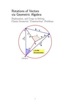
  • 22. As a contrast that might prove useful, this problem is solved without using rotations in ”Find tangents to a circle from a point, using Geometric Algebra” (as GeoGebra worksheet, as YouTube video). 4.2 Problem 2 Derive an equation for the position of the circumcenter of a triangle with respect to one of its vertices. Identifying Potentially Useful Elements of the Problem This problem can be solved in several different ways. For example, because the mediatrix of any chord in a circle passes through the circle’s center (1 ), we can find the circumcenter of our triangle by finding the point at which the mediatrices of any two sides of the triangle intersect. We can also find the circumcenter via simple trigonometry. However, we wish to solve this problem by using rotations, so let’s begin by asking, ”Is the circumcenter involved in the rotation of any identifiable vectors?” As soon as we add the circumcenter to our previous diagram, and draw vectors from the circumcenter to any two of the given triangle’s vertices, 22
  • 23. Two methods of solving problems via rotations: • Equate two expressions for the same angle (in this case, α); and • Write one vector as a ”rotation + dilation” of the other. In this case, c − q is a pure rotation of b − q because both are radii of the same circle. Quite often, the equation obtained via one of these methods is much easier to solve than that obtained via the other. we can see that the required circle converts the given triangle into ”three in- scribed angles” (5). Therefore, we can choose any of the triangle’s vertices the origin (we’ve chosen a), and write α = 2θ, from which eθi eθi = e2θi . Formulating a Strategy One strategy is to express the equality of angles that we’ve just identified in terms of products of vectors, in order to obtain an equation involving q: eαi = e2θi eαi = eθi eθi b − q |b − q| c − q |c − q| = ˆbˆc ˆbˆc . Then, we’d expand both sides of the equation that we’ve just obtained, after which we’d use other manipulations to identify q. We’ll use that strategy in later problems, but before we dive into it here, we should also note that c − q is a pure rotation of b − q because both are radii of the same circle: [b − q] eαi = c − q [b − q] eθi eθi = c − q [b − q] ˆbˆc ˆbˆc = c − q, b ˆbˆc ˆbˆc = bˆb ˆcˆbˆc = |b| ˆcˆbˆc = ˆc |b| ˆb ˆc = ˆcbˆc. from which b ˆbˆc ˆbˆc − q ˆbˆc ˆbˆc = c − q, q − q ˆbˆc ˆbˆc = c − b ˆbˆc ˆbˆc , q 1 − ˆbˆcˆbˆc = c − b ˆbˆc ˆbˆc q 1 − ˆbˆcˆbˆc = c − ˆcbˆc. 23
  • 24. Is that result helpful? Yes, because 1− ˆbˆcˆbˆc has a multiplicative inverse in GA. Therefore, we can write the following in a purely formal way, then identify what that inverse is, precisely: q 1 − ˆbˆcˆbˆc 1 − ˆbˆcˆbˆc −1 = (c − ˆcbˆc) 1 − ˆbˆcˆbˆc −1 ∴ q = (c − ˆcbˆc) 1 − ˆbˆcˆbˆc −1 . Appendix A (p. 60) solves for q in this way. Although it’s more complicated than the ways that we’ll see here shortly, it’s recommended (along with the comments thereon) for its time-saving pointers regarding inverses of multivectors, and for its observations on geometric interpretation of results and transformations of vectors. However, is there an even-easier way? Let’s add a few more elements to our diagram, then examine it again: We see now that a rotation through our angle θ, in combination with a dilation by the scalar factor |d − q| |b − q| , will transform the vector b − q into d − q: d − q = |d − q| |b − q| (b − q) eθi = |d − q| |b − q| (b − q) ˆbˆc. The next few paragraphs indicate how we’d use ordinary trigonometry to identify the position of the incenter with respect to the midpoint of segment bc. Note also that |b − c| 2 = |b − d| = |b − q| ˆbi · ˆc ∴ |b − q| = |b − c| 2 ˆbi · ˆc . Determining the value of |d − q| |b − q| is easy enough: d − q is the projection of b − q upon (b − c) i, so |d − q| = |b − q| cos θ = |b − q| ˆb · ˆc; ∴ |d − q| |b − q| = ˆb · ˆc. Putting these observations and results together, our equation d − q = |d − q| |b − q| (b − q) ˆbˆc 24
  • 25. becomes d − q = ˆb · ˆc (b − q) ˆbˆc. To solve that equation for q, we rearrange it as q ˆb · ˆc ˆbˆc − 1 = ˆb · ˆc ˆbˆc − d, then right-multiply both sides by ˆb · ˆc ˆbˆc − 1 −1 . That task promises to be somewhat easier than finding q via the equation that we obtained previously, which was q = (c − ˆcbˆc) 1 − ˆbˆcˆbˆc −1 . Still, we can do even better. Let’s recall the first strategy that we identified for finding q: that of writing the rotation operator e2θi as the product of the unit vector in the direction b−q and the unit vector in the direction c−q. Combining that idea with the experience we’ve gained subsequently from formulating two alternative strategies, we can see potential benefit in writing The unit vector in the direction (b − c) i is the rotation, through the angle θ, of the unit vector in the direction b − q. That is, (b − c) i |b − c| = b − q |b − q| eθi From our previous work, we can derive that |b − q| |b − c| = 1 2 ˆbi · ˆc . from which |b − q| |b − c| (b − c) i = (b − q) ˆbˆc, and qˆbˆc = bˆbˆc −   (b − c) i 2 ˆbi · ˆc   = |b| ˆc −   (b − c) i 2 ˆbi · ˆc  . That equation is the one that we shall now solve. Solving the Equation In the equation qˆbˆc = |b| ˆc −   (b − c) i 2 ˆbi · ˆc  , 25
  • 26. q is right-multiplied by ˆbˆc . We can undo those operations by right-multiplying by ˆcˆb, which of course happens to be ˆbˆc −1 : qˆbˆc ˆcˆb = |b| ˆc −   (b − c) i 2 ˆbi · ˆc   ˆcˆb q = |b| ˆcˆcˆb −  (b − c) ˆicˆb 2 ˆbi · ˆc   = b +  cˆcˆb − bˆcˆb 2 ˆbi · ˆc  i = b +   |c| ˆb − b 2ˆc · ˆb − ˆbˆc 2 ˆbi · ˆc  i = b +   |c| ˆb + |b| ˆc − 2 ˆb · ˆc b 2 ˆbi · ˆc  i Appendix A (p. 60) discusses in detail many aspects of finding inverses of multivectors. One quick way to see that ˆbˆc −1 is ˆcˆb is by noting that ˆbˆc = eθi , the multiplicative inverse of which is e−θi , which in turn, as we can deduce from our diagrams, is ˆcˆb. This answer is satisfactory for computing q, but we can transform it into a version that’s more useful and informative. Interpreting the Solution, and Transforming It into a More-Useful Form Readers are encouraged to review the extensive treatment that this subject is given in Appendix A (p. 60), for the version of the solution obtained by solving the equation q = (c − ˆcbˆc) 1 − ˆbˆcˆbˆc −1 . Here, we’ll transform the solution that we just obtained into a form that shows that q lies along the mediatrix of segment bc. We begin the transformation by going back a few steps to q = b +  cˆcˆb − bˆcˆb 2 ˆbi · ˆc  i, 26
  • 27. then continuing q = b +   cˆcˆb − b 2ˆb · ˆc − ˆbˆc 2 ˆbi · ˆc  i = b +   cˆcˆb + bˆbˆc − 2 ˆb · ˆc b 2 ˆbi · ˆc  i = b +   c ˆc · ˆb + ˆc ∧ ˆb + b ˆb · ˆc + ˆb ∧ ˆc − 2 ˆb · ˆc b 2 ˆbi · ˆc  i = b +   (c − b) ˆb · ˆc + (b − c) ˆb ∧ ˆc 2 ˆbi · ˆc  i = b +   (c − b) ˆb · ˆc + (b − c) ˆbi · ˆc i 2 ˆbi · ˆc  i = b +   ˆb · ˆc ˆbi · ˆc   c − b 2 i + c − b 2 = b + c 2 + ˆb · ˆc ˆb · (ˆci) b − c 2 i . The geometric significance of that version is shown in the following figure: As we knew from the classical solution and from trigonometry, q lies along the mediatrix of segment bc. 4.3 Problem 3 Derive an equation for the position of the incenter of a triangle with respect to one of its vertices. 27
  • 28. Identifying Potentially Useful Elements of the Problem Although the problem is posed as one of finding the incenter, we can see that each of the triangle’s vertices is a point from which tangents are drawn to the required circle. Thus, we have three cases of Problem 1 (4.1). So, let’s choose one of the vertices as the origin, then identify elements that might be useful. One key fact is that from Problem 1, we know that the incenter must lie along the bisector of the angle formed by the tangents drawn to the circle. Thus the incenter lies along the direction ˆb + ˆc 2 . A second is that the radii from the incenter to the points of tangency are perpendicular to the triangle’s sides. A third is that the lengths of the tangents from each vertex are equal. From the latter, we can deduce that the length of the segment cb is equal to the sum of the lengths of segments cg and bf. We can also see several rotations that we might be able to formulate via GA and use to find the answer, so let’s add a few more elements to our figure so that we can treat those rotations more precisely. 28
  • 29. Although we drew this diagram in order to examine rotations, we can see that it also helps us refine our initial observations about lengths of segments. Why not do so now, before moving on to the rotations? We noted that the sides of the triangle are perpendicular to the radii drawn from the incenter, so we know that vector f is q’s projection upon ˆb: f = q · ˆb ˆb. Because the two tangents drawn to a circle from a given point are equal in length, we know that |g| = |f|. Therefore, g = q · ˆb ˆc. Our initial observation that the length of segment bc is the sum of the lengths of segments cg and bf can also be translated into a ”GA-friendly” vector equation: |c − b| = |g − c| + |f − b| = |c| − |g| + |b| − |f| = |c| − q · ˆb + |b| − q · ˆb. Therefore, q · ˆb = |b| + |c| − |c − b| 2 . That result is sure to be important; we could solve for q immediately if we knew the geometric product qˆb, and all we need to do in order to form that product is to determine the outer product q ∧ ˆb. That outer product will probably arise somewhere in the expressions for rotations that we intend to examine, so let’s turn to those now. 29
  • 30. One of those rotations is that of vector f through the angle θ to give vector g: g = feθi , with eθi = ˆbˆc. A more-exotic example is illustrated by the following diagram. We express the vector h in two ways: as q plus the rotation of f − q through the angle β, h = q + (f − q) eβi . and as the vector b plus the rotation of f − b through the angle ψ: h = b + (f − b) eψi . 30
  • 31. The rotation operator eψi can be written as the geometric product −ˆb c − b |c − b| = |b| − ˆbc |c − b| . To derive an expression for β, we use the theorem about the measure of an angle drawn from a point exterior to a circle (p. 11). The angles β and δ are shown as negative (clockwise) angles in our diagram, so β + δ = −2π. Therefore, ψ = 1 2  β − (−2π − β) =δ   , = β + π, from which β = ψ − π (which is clearly a negative angle). These observations appear to have provided enough information —and in ”GA-friendly form”—to solve the problem, so let’s formulate a strategy. Formulating a Strategy Our observations have suggested two strategies: 1. Identify q from the known value of q · ˆb and from the value of q · ˆb, which is still unknown, but which we should be able to determine by analyzing rotations; and 2. Although the solution via the second strategy is not presented in this document, that strategy does work. Equating the two expressions for h gives q + (f − q) eβi = b + (f − b) eψi , q + (q − f) eψi = b + (f − b) eψi , and q (1 + b) eψi = b 1 − eψi + 2feψi . From there, we’d right-multiply both sides by 1 + eψi −1 to solve for q . See Appendix A (p. 60) for the method. Equate the two expressions that we obtained for the vector h: h = b + (f − b) eψi . and h = q + (f − q) eβi . with f = q · ˆb ˆb = |b| + |c| − |c − b| 2 ˆb, and eβi = e(ψ−π)i = eψi e(−π)i =−1 = −eψi = ˆbc − |b| |c − b| . An important piece of information that neither of our strategies uses. We’ll use the first strategy because it appears to be simpler. However, this is a good moment to note that neither of the strategies makes use of an important observation that we made earlier: the point q lies along the direction ˆb + ˆc 2 . We can express that observation in terms such as q ∧ ˆb + ˆc = 0, and q ∧ ˆb + q ∧ ˆc = 0. Let’s summarize the information that we’ve identified as relevant to the strategy we’ve chosen: 31
  • 32. q · ˆb = |b| + |c| − |c − b| 2 q ∧ ˆb + ˆc = 0, or equivalently, q ∧ ˆb + q ∧ ˆc = 0. Having formed q ∧ ˆb + ˆc so easily, and recognizing that we’d need to work a bit to find q∧ˆc, we might ask now whether we’d be better off finding q· ˆb + ˆc , so that we can then find q from the geometric product q ˆb + ˆc . This moment in our solution process is where our initial exploration of lengths of segments pays off: we found that |g| = |f| = q · ˆb = |b| + |c| − |c − b| 2 . That additional information makes the route clear to us: q · ˆb + ˆc = q · ˆb + q · ˆc = |b| + |c| − |c − b| ; q ∧ ˆb + ˆc = 0; ∴ q ˆb + ˆc = q · ˆb + q · ˆc = |b| + |c| − |c − b| . We’ll find q by solving that equation. Solving the Equation Our equation is q ˆb + ˆc = q · ˆb + q · ˆc = |b| + |c| − |c − b|, which we solve via q ˆb + ˆc ˆb + ˆc −1 = [|b| + |c| − |c − b|] ˆb + ˆc −1 q = [|b| + |c| − |c − b|]    ˆb + ˆc ˆb + ˆc 2    = [|b| + |c| − |c − b|] ˆb + ˆc 2 + 2ˆb · ˆc = |b| + |c| − |c − b| 1 + ˆb · ˆc ˆb + ˆc 2 . Interpreting the Solution The incenter lies along the bisector of the angle formed by sides b and c, at a distance from point a equal to |b| + |c| − |c − b| 1 + ˆb · ˆc times the length of ˆb + ˆc 2 . Because the assumptions that we made about the vertex a apply to all three vertices of any triangle, our solution is valid for all vertices of every triangle. Therefore, the incenter is the point of intersection of the bisectors of the three angles formed by the sides of the triangle. This result is the same as that obtained via classical geometry. 32
  • 33. 4.4 Problem 4 Given two circles, and a point p on one of them, construct the circles that are tangent to both of the given circles, with p being one of the points of tangency. This problem has two solutions (i.e., the red and magenta circles). We’ll find them in four ways, using two different concepts. 4.4.1 Solution Concept 1 In this first solution, we won’t think about the problem in terms of rotating vectors; instead, we’ll use the expressions that we’ve developed as a means of expressing angles between pairs of vectors in a convenient way. From there, we’ll go on to solve for the vectors from the origin to the points of tangency between the given circles and the ones that we’re asked to construct. Please note that the solution presented here, although it uses the same ideas as the one presented in ”Answering Two Common Objections to Geometric Algebra” (on YouTube, on GeoGebraTube), is considerably ”cleaner” because we’re using the starting point of the vectors t1 and t2 is used as the origin, rather than the center of the circle on which p is located. 33
  • 34. The angle between the directions of vectors t1 and p−t1 is θ, in the positive (i.e., ccw) direction. Because the triangle pt1c2 is isosceles, the angle between the directions of t1 −p and p−c2 is θ as well. Also, |t1| = r1, and |p − c2| = r2. Therefore, t1 (p − t1) = |t1| |p − t1| eθi = r1 |p − t1| eθi ; and (t1 − p) (p − c2) = |t2| |p − c2| eθi = r2 |p − t1| eθi , from which (t1 − p) (p − c2) = r2 r1 t1 (p − t1) . Additional details on the maneuvers needed here can be found in Appendix C (page 74 ) and in ”Answering Two Common Objections to Geometric Algebra”: On YouTube On GeoGebraTube. In those sources, you’ll also find other ways to solve such equations. Expanding both sides, recognizing that t2 1 = r2 1, and rearranging, we obtain t1 r2 r1 − 1 p + c2 = r1r2 + pc2 − p2 . Now, we right-multiply both sides by the inverse of r2 r1 − 1 p + c2 to solve for t1. (Recall that the inverse of a vector v is v/ |v| 2 .) After rearranging the right-hand side, we arrive at t1 = r2 2 − r1r2 + c2 2 − r2 r1 − 1 p2 + 2 r2 r1 − 1 p · c2 p + r1r2 − r2 r1 p2 c2 r2 r1 − 1 2 p2 + c2 2 + 2 r2 r1 − 1 p · c2 . To find t2, we recognize that the angles φ are equal. 34
  • 35. Using the same ideas as in the solution for t1, we write −t2 (p − t2) = |−t2| |p − t2| eφi = r1 |p − t2| eφi ; and (t2 − p) (p − c2) = |t2| |p − c2| eφi = r2 |p − t1| eφi , which leads to t2 r2 r1 + 1 p − c2 = r1r2 − pc2 + p2 , and t2 = r2 2 + r1r2 + c2 2 + r2 r1 + 1 p2 − 2 r2 r1 + 1 p · c2 p + r2 r1 p2 − r1r2 c2 r2 r1 + 1 2 p2 + c2 2 − 2 r2 r1 + 1 p · c2 . You’ve probably been thinking that the problem asks us to do more than find t1 and t2: we’re required to identify (that is, to give equations for) the tangent circles. So, now that we’ve found the points of tangency, how do we proceed? 35
  • 36. We can also express e α 2 i directly in terms of the vectors c2 − p and t2. See page 16 . One possibility is given in Hestenes D. 1999, pp. 88-89. We’ll use the magenta circle as our example. Knowing t2, we can determine the angle α. Thus, we know that every point x on the magenta circle satisfies the condition expressed by the equation (p − x) −1 (t2 − x) = δe α 2 i , where δ is a scalar, −∞ < δ < ∞ . To each finite value of δ, there corresponds a unique point x; the absolute value of δ increases without limit (”goes to infinity”) as x approaches p. 4.4.2 Solution Concept 2 In our second Solution Concept, we makes life more difficult for ourselves—deliberately—in order to demonstrate ideas that will prove helpful in more-difficult problems later on. We begin by re-examining our figure, and noting from plane geome- try, the angle between the vectors p − c3 and t1 − c3 is 2ψ. 36
  • 37. Thus t1 − c3 = (p − c3) e2ψi . To obtain an expression for eψi , we can use either [− (p − c2) i] (t1 − p) |(−p − c2| i| |t1 − p| or (p − t1) t1i |p − t1| |t1i| . We’ll opt for the latter, because it promises to be simpler to use. From the preceding, we can see that we can obtain the vector t1 − c3 by rotating the vector p − c3 counterclockwise through the angle ψ twice: (p − c3) eψi eψi = t1 − c3. A word about what we’re working toward here: We’re going to try to form an equation in which one side is a product of vectors, and the other is either a pure scalar or a pure bivector. Then, we’ll use postulates about the equality of multivectors to obtain an equation that we can solve simply for t1. That information doesn’t appear useful until we recognize that p − c3 = − r3 r2 (p − c2), and t1 − c3 = − r3 r1 t1. Making these substitutions, and using the expression that we chose for eψi , the previous equation becomes − r3 r2 (p − c2) =p−c3 (p − t1) t1i |p − t1| |t1i| (p − t1) t1i |p − t1| |t1i| = − r3 r1 t1. We can simplify that result, using |t1i| = r1, thereby finding that (p − c2) (p − t1) t1i (p − t1) t1i = r1r2 |p − t1| 2 t1. ”Switching places of i’s and vectors” is a common and important maneuver that we’ll use many times in this document. You’ll learn to simplify it quite soon: just examine the term on which you’re working, and count the number of ”switches” that will be needed to bring the i’s together within that term to make a ”-1”. That is, an ”i2 ”. If that number is even, then the sign of the term inverts; if odd, the sign remains unchanged. In the present example, we made two switches, so the sign inverted. Next, we eliminate the two factors i on the left-hand side by ”bringing them together”. To do so, we just make a series of ”switches” of place between one of the i’s and an adjacent vector. We use the identify iv ≡ −vi to keep track of sign changes: (p − c2) (p − t1) t1i (p − t1) t1i = r1r2 |p − t1| 2 t1 Repeating the previous equation , 37
  • 38. − (p − c2) (p − t1) t1 (p − t1) i 1st switch t1i = r1r2 |p − t1| 2 t1, (p − c2) (p − t1) t1 (p − t1) t1i 2nd i = r1r2 |p − t1| 2 t1, (p − c2) (p − t1) t1 (p − t1) t1i2 = r1r2 |p − t1| 2 t1, (p − c2) (p − t1) t1 (p − t1) (−1) = r1r2 |p − t1| 2 t1, (p − c2) (p − t1) t1 (p − t1) = −r1r2 |p − t1| 2 t1. The key equation for Concept 2 Right-multiplying now by t1 −1 , we obtain the key equation for Concept 2: (p − c2) (p − t1) t1 (p − t1) = −r1r2 |p − t1| 2 . The right-hand side is a scalar. That result deserves several comments. The first is that as we saw earlier, the geometric product of any three coplanar vectors is another vector in the same plane. Therefore, the geometric product of any four coplanar vectors is the sum of a scalar and a bivector, only. More to the point, because (p − c2) (p − t1) t1 (p − t1) evaluates to a scalar, its bivector part is zero: (p − c2) (p − t1) t1 (p − t1) 2 = 0. We’ll see, shortly, how to make use of that fact, but first let’s note an- other important aspect of our key equation: it contains the sequence of factors (p − t1) t1 (p − t1), which is of the form uvu. That’s noteworthy because for any two vectors v and ˆu, the product ˆuvˆu is the reflection of v with respect to ˆu. Hence, (p − t1) t1 (p − t1) is the reflection of t1 with respect to (p − t1), and multiplied by the factor |p − t1| 2 . Based upon those observations, and upon |p − c2| = r2 and t1 = r1, we can see that the equation (p − c2) (p − t1) t1 (p − t1) = −r1r2 |p − t1| 2 tells us that (p − t1) t1 (p − t1) is equal to |p − t1| 2 t1 in magnitude, and is parallel to p − c2, but opposite in direction. Now that we’ve discussed some of the geometric significance of the equation (p − c2) (p − t1) t1 (p − t1) = −r1r2 |p − t1| 2 , we’ll solve that equation in three ways. Concept 2, Solution Method 1 As noted above, the right-hand side of our key equation (Page 38) (p − c2) (p − t1) t1 (p − t1) = −r1r2 |p − t1| 2 Now we see why we wanted (p. 37) an equation in which one side was either a pure scalar or a pure bivector: The left-hand side of our key equation is the product of an even number of vectors, so it must evaluate to a multivector that’s the sum of a scalar and a bivector. Because the right-hand side is a pure scalar, the bivector part of the left-hand side must be zero. is a scalar. Therefore, (p − c2) (p − t1) t1 (p − t1) 2 = 0. 38
  • 39. To use that fact, we’ll begin by expanding the left-hand side, then simpli- fying. (Again, t2 1 = r2 1.) (p − c2) (p − t1) t1 (p − t1) = ppt1p − ppt1t1 − pt1t1p + pt1t1t1 − c2pt1p +c2pt1t1 + c2t1t1p − c2t1t1t1 = p2 t1p − 2r1 2 p2 + r1 2 pt1 − c2pt1p + 2r1 2 c2p −r1 2 c2t1. Now, we need to identify the bivector part of the simplified expansion. The bivector part of a sum of terms is the sum of the terms’ respective bivector parts. (Note that r1 2 p2 is a scalar, so its bivector part is zero.) The only term whose bivector part might cause us some trouble is c2pt1p. What is c2pt1p 2? Several different ways of identifying it are presented in the Appendix (7.2). The most straightforward way uses the identity that for any two vectors u and v, uv ≡ 2u · v − vu. Therefore, c2pt1p 2 = c2 (2p · t1 − t1p) p 2 = 2 (p · t1) c2p − p2 c2t1 2 = 2 (p · t1) c2 ∧ p − p2 c2 ∧ t1. An important identity that’s useful in solving equations that arise when working with rotations: u ∧ v = [(ui) · v] i = − [u · (vi)] i. Using this expression, and our identity that for any two vectors u and v, u ∧ v = [(ui) · v] i, we arrive at (p − c2) (p − t1) t1 (p − t1) 2 = p2 − r1 2 c2 ∧ t1 − p2 − r1 2 p ∧ t1 −2 (p · t1) c2 ∧ p + 2r1 2 c2 ∧ p = p2 − r1 2 [(c2i) · t1] i − p2 − r1 2 [(pi) · t1] i −2 (p · t1) [(c2i) · p] i + 2r1 2 [(c2i) · p] i. Now, we can make use of the fact that (p − c2) (p − t1) t1 (p − t1) 2 is zero: p2 − r1 2 [(c2i) · t1] i − p2 − r1 2 [(pi) · t1] i − 2 (p · t1) [(c2i) · p] i + 2r1 2 [(c2i) · p] i = 0, which (after eliminating the factor i) we can rearrange as follows : [2 (c2i) · p] p + p2 − r2 1 (pi − c2i) W e ll call this vector ”z” ·t1 = 2r2 1 (c2i) · p. Therefore, t1 · ˆz = 2r2 1 (c2i) · p |z| . That result is useful to us because we also know that t1 = (t1 · ˆz) ˆz + [t1 · (ˆzi)] ˆzi, and t2 1 = r2 1. From those facts, we can show that t1 · (ˆzi) = ± r2 1 − (t1 · ˆz) 2 . 39
  • 40. But which root is correct: the positive, or the negative? To answer that ques- tion, let’s attempt to identify the vector t2. Looking again at our diagram, we find that (p − c4) e2ϕi = t2 − c4. Proceeding now in the same way that we did to find t1, − r4 r2 (p − c2) eϕi eϕi = r4 r1 t2 − r4 r2 (p − c2) (p − t2) (−t2i) |p − t2| |−t2i| =eϕi (p − t2) (−t2i) |(−t2i)| |−t2i| = r4 r1 t2 (p − c2) (p − t2) t2 (p − t2) t2 = r2 r1 |p − t2| 2 |t2| 2 t2 Therefore, (p − c2) (p − t2) t2 (p − t2) = r1r2 |p − t2| 2 . Let’s compare that equation to the corresponding one that we obtained for t1 (Page 38): (p − c2) (p − t1) t1 (p − t1) = −r1r2 |p − t1| 2 The right-hand sides of the two equations have opposite algebraic signs. Those signs, plus the fact that the right-hand sides are scalars, tell us that the vector (p − t2) t2 (p − t2) is parallel to p − c2, while the vector (p − t1) t1 (p − t1) is anti-parallel to it. Therefore, t1 and t2 are not the same vector. Nevertheless, both of those vectors have the same length (= r1), and both have the same projection upon z, as we can show by recognizing that (p − c2) (p − t2) t2 (p − t2) 2 = 0, then proceeding as we did for t1. In this way we arrive at [2 (c2i) · p] p + p2 − r2 1 (pi − c2i) T his is the same vector ”z” as for t1 ·t2 = 2r2 1 (c2i) · p =t1·z , 40
  • 41. ∴ t2 · ˆz = 2r2 1 (c2i) · p |z| = t1 · ˆz. Their components perpendicular to z are of equal length = r2 1 − (t1 · ˆz) 2 , but are oppositely directed. (That’s why the vectors (p − t2) t1 (p − t1) and (p − t2) t2 (p − t2) are oppositely directed.) Therefore, the solution obtained by using the present method is t = 2r2 1 (c2i) · p |z| ˆz ±    r1 2 − 2r2 1 (c2i) · p |z| 2    ˆzi, where z = [2 (c2i) · p] p + p2 − r2 1 (pi − c2i) . That form of the solution is satisfactory for computing t; if we wished, we could transform it into another form by using ideas presented in the work- sheet and video, ”Find unknown vector from two dot products” (as GeoGebra worksheet , as YouTube video). Concept 2, Solution Method 2 We’ll start from our key equation for this concept (Page 38): (p − c2) (p − t1) t1 (p − t1) = −r1r2 |p − t1| 2 . In Solution Method 1 for this concept, we used the fact that the left- hand side evaluates to a scalar, and thereby arrived at an equation for the dot product t1 ·z. However, we made no use of the fact the left-hand side evaluates to the specific scalar −r1r2 |p − t1| 2 . In the present Method, we’ll use that information to find t1’s dot product with a second vector, which we’ll call ˆw1. Knowing t1’s dot products with those two vectors, we’ll be able to find t1 using methods developed in the worksheet and video, ”Find unknown vector from two dot products” (As GeoGebra worksheet , As YouTube video). 41
  • 42. From Method 1, we also know that (p − c2) (p − t1) t1 (p − t1) can be ex- panded as (p − c2) (p − t1) t1 (p − t1) = p2 t1p + r1 2 pt1 − r1 2 c2t1 + 2r1 2 c2p − 2r1 2 p2 − 2 (p · t1) c2p − p2 c2t1 =c2pt1p . Because |p − t1| 2 is (p − t1) 2 , p2 t1p + r1 2 pt1 − r1 2 c2t1 + 2r1 2 c2p − 2r1 2 p2 − 2 (p · t1) c2p − p2 c2t1 = −r1r2 p2 − 2p · t1 + r1 2 =(p−t1)2 . Equating the scalar parts of the two sides, and rearranging, we obtain p2 + r1 2 − 2 (r1r2 + c2 · p) p + p2 − r1 2 c2 W e ll call this w1. ·t1 = 2r1 2 p2 − c2 · p −r1r2 p2 + r1 2 . Similarly, starting from (p − c2) (p − t2) t2 (p − t2) = r1r2 |p − t2| 2 , we find that p2 + r1 2 + 2 (r1r2 − c2 · p) p + p2 − r1 2 c2 W e ll call this w2. ·t2 = 2r1 2 p2 − c2 · p +r1r2 p2 + r1 2 . We now have a pair of ”dot-product” equations for each of the vectors t1 and t2: z · t1 = 2r2 1 (c2i) · p, w1 · t1 = 2r1 2 p2 − c2 · p − r1r2 p2 + r1 2 . z · t2 = 2r2 1 (c2i) · p, w2 · t2 = 2r1 2 p2 − c2 · p + r1r2 p2 + r1 2 . In the worksheet and video ”Find unknown vector from two dot products”, we learned that given the dot products of an unknown vector x with two known vectors a and b, we can find x by writing it as a linear combination of a and b, x = αa + βb, from which we can then form the pair of linear equations a · x = αa2 + βa · b, b · x = αa · b + βb2 . 42
  • 43. Solving those equations for α and β, we obtain α = b2 a · x − (a · b) (b · x) a2b2 − (a · b) 2 , β = a2 b · x − (a · b) (a · x) a2b2 − (a · b) 2 . Making use of that solution, we find that t1 = α1w1 + β1z, where α1 = z2 w1 · t1 − (w1 · z) (z · t1) w1 2z2 − (w1 · z) 2 , β = w1 2 z · t1 − (w1 · z) (w1 · t1) w1 2z2 − (w1 · z) 2 , w1 = p2 + r1 2 − 2 (r1r2 + c2 · p) p + p2 − r1 2 c2, w2 = p2 + r1 2 + 2 (r1r2 − c2 · p) p + p2 − r1 2 c2, z = [2 (c2i) · p] p + p2 − r2 1 (pi − c2i), w1 · t1 = 2r1 2 p2 − c2 · p − r1r2 p2 + r1 2 , w1 · t2 = 2r1 2 p2 − c2 · p + r1r2 p2 + r1 2 , z · t1 = z · t2 = 2r2 1 (c2i) · p. Concept 2, Solution Method 3 Anyone who’s studied Geometric Alge- bra—even casually—knows that the method usually prescribed for solving for an unknown vector x in a given problem is to find x’s inner and outer products with a known vector b, then proceed as follows: x · b + x ∧ b = xb x = (xb) b−1 Very antiseptic-looking! However, in this section, we’ll learn that x·b and x∧b can take quite-complicated forms. As we did in previous sections, we’ll start with our key equation: (p − c2) (p − t1) t1 (p − t1) = −r1r2 |p − t1| 2 . Again, we’ll expand the left-hand side. But this time, we’ll maintain p−c2 intact, as a single factor: (p − c2) pt1p − 2r1 2 p + r1 2 t1 =(p−t1)t1(p−t1) = −r1r2 |p − t1| 2 . 43
  • 44. Examining the left-hand side, we see an interesting possibility: if we left- multiply by (p − c2) −1 , and right-multiply by p, we’ll obtain a sum of three terms: a scalar, and two terms that are scalar multiples of geometric products of p and t1. On the right-hand side, we’ll obtain a scalar multiple of the product (p − c2) p: (p − c2) −1 (p − c2) pt1p − 2r1 2 p + r1 2 t1 p = (p − c2) −1 −r1r2 |p − t1| 2 p p2 pt1 + r1 2 t1p − 2r1 2 p2 = − r1r2 |p − t1| 2 (p − c2) 2 (p − c2) p = r1r2 |p − t1| 2 (p − c2) 2 c2p − p2 . Now, we can develop expressions for t1 · p and t1 ∧ p. Equating the scalar parts of both sides, and solving for t1 · p, we find that t1 · p = 2r1 2 p2 (p − c2) 2 − r1r2 p2 + r1 2 p2 − c2 · p (p2 + r1 2) (p − c2) 2 − 2r1r2 (p2 − c2 · p) . Equating the bivector parts of both sides, we obtain t1 ∧ p = r1r2 p2 − 2t1 · p + r1 2 (p2 − r1 2) (p − c2) 2 [(pi) · c2] i =p∧c2 . Note that our expression for t1 ∧p contains the quantity t1 ·p. That’s fine, because the expression for t1 ·p allows us to calculate the value of t1 ·p directly from known quantities (r1, r2, p, and c2), after which we’d use that value to calculate t1 ∧ p. If we wished, we could also do the work symbolically. That is, we could substitute our expression for t1 · p into our expression for t1 ∧ p, then do the algebra to obtain an expression for t1 ∧ p in terms of the known quantities. Having obtained these expressions for t1 · p and t1 ∧ p, how do we use them to determine t1? This is where we need to understand the meaning of the symbol ”+” in the ”antiseptic” version of the solution t1 · p + t1 ∧ p = t1p t1 = (t1p) p−1 . We’ll see a brief explanation here; more details are given in the worksheet and video ”Answering Two Common Objections to Geometric Algebra” (As GeoGebra worksheet , As YouTube video). To solve for t1, starting from the preceding equations, we write t1 = (t1 · p + t1 ∧ p) =t1p p−1 = (t1 · p) p−1 + (t1 ∧ p) p−1 = t1 · p p2 p + t1 ∧ p p2 p. 44
  • 45. Every exterior product (including t1 ∧ p) is a scalar multiple of the unit bivector i. Therefore, the second term on the right-hand side of the above equation is a scalar multiple of ip, which is a vector. For that reason, the second term is also a scalar multiple of −pi, where pi is the 90◦ counter- clockwise rotation of p. Therefore, the solution t1 = t1 · p p2 p + t1 ∧ p p2 p expresses t1 as a linear combination of the vectors p and pi. The analysis that we’ve just seen shows why we can view the operation represented by the symbol ”+” in the definition x · b + x ∧ p = xb as a ”latent vector addition” that becomes ”activated” when right-multiplied by a vector. When multiplied by the vector b−1 , the result is x. With that understanding, we can see how to put the product (t1 ∧ p) p−1 into a form that’s useful to us: (t1 ∧ p) p−1 = r1r2 p2 − 2t1 · p + r1 2 (p2 + r1 2) (p − c2) 2 [(pi) · c2] i p p2 =p−1 = − r1r2 p2 − 2t1 · p + r1 2 p2 (p2 + r1 2) (p − c2) 2 [(pi) · c2] pi. Therefore, the solution given by the present method is t1 · p =    2r1 2 p2 (p − c2) 2 − r1r2 p2 + r1 2 p2 − c2 · p p2 (p2 + r1 2) (p − c2) 2 − 2r1r2 (p2 − c2 · p)    =(t1·p)/p2 p − r1r2 p2 − 2t1 · p + r1 2 p2 (p2 + r1 2) (p − c2) 2 [(pi) · c2] pi. Again, this solution could be simplified algebraically. (We’ll omit the solu- tion for t2.) 4.5 Problem 5 Given a circle and two points outside of it, identify the circles that are tangent to the given one, and that pass through both of the given points. 45
  • 46. We’ll see three ways to arrive at equations that can be solved for the points of tangency by using Method 1 from Problem 4, Concept 2 (4.4.2). 4.5.1 Solution Concept 1 How would we proceed after identifying the points of tangency? As is known from classical geometry, we can construct a circle if we know any three points that lie on it. One of the GA expressions of that truth is that if c, d, and e are three known points on a circle, then every other point x on that circle must satisfy the condition expressed by the ”cross-ratio” equation (c − x)−1 (d − x) (c − e)−1 (d − e) = a scalar. For details, see Hestenes D. 1999, p. 89. In our case, for the circle that contains t1, the known points would be a, b, and t1, so one version of the cross-ratio equation for that circle would be (a − x)−1 (b − x) (a − t1)−1 (b − t1) = ascalar. Other versions can be obtained by interchanging a, b, and t1. This way is the simplest: we’ll begin by identifying the elements shown in the following figure: Now, we obtain two expressions for eθi , and equate them to each other. We’ll use the fact that |t1i| = |t1| = r: (a − b) (t1 − b) |a − b| |t1 − b| = (a − t1) t1i |a − t1| |t1i| Both sides are expressions for eθi . Next, we form an equation in which one side is a product of the vectors that are involved, and the other side is either a scalar or a bivector: 46
  • 47. (a − t1) (a − b) (t1 − b) |a − b| |t1 − b| t1i = (a − t1) (a − t1) t1i |a − t1| |t1i| t1i (a − t1) (a − b) (t1 − b) t1i (−i) = |a − t1| |t1 − b| (a − t1) r (−i) (a − t1) (a − b) (t1 − b) t1 = − |a − t1| |t1 − b| (a − t1) ri. The right-hand side is a bivector, so (a − t1) (a − b) (t1 − b) t1 0 = 0. A convenient way to expand (a − t1) (a − b) (t1 − b) t1 is via a2 − ab − t1a + t1b t1 2 + t1b , which works out to b2 − r2 at1 − a2 − r2 bt1 + r2 a2 − b2 − r2 ab + t1abt1. Therefore, b2 − r2 at1 − a2 − r2 bt1 + r2 a2 − b2 − r2 ab + t1abt1 0 = 0. The term t1abt1 is interesting. At the beginning of 4.4.2, we saw that the product ˆuvˆu evaluates to a vector: specifically, the reflection of v with respect to ˆu. Similarly, the product ˆuvwˆu is the reflection of the geometric product vw. But let’s see exactly why that is, and what it means. We’ll discover that the scalar part of vw: is unaffected by the reflection, but the bivector part is reversed, so that ˆuvwˆu = wv: ˆuvwˆu = ˆu (v · w + v ∧ w) ˆu = ˆu (v · w) ˆu + ˆu (v ∧ w) ˆu = ˆu2 (v · w) + ˆu [(vi) · w] iˆu = v · w + ˆu [−v · (wi)] (−ˆui) = v · w + ˆu2 [(wi) · v] i = w · v + w ∧ v = wv. Another interesting aspect of the product ˆuvwˆu is that the reflection of the exterior product of v and w is equal to the exterior product of the two vectors’ reflections: ˆuvwˆu = ˆuv (ˆuˆu) wˆu = (ˆuvˆu) (ˆuwˆu) . That observation provides a geometric interpretation of why reflecting a bivector changes its sign: the direction of the turn from v to w reverses. 47
  • 48. Returning now to t1abt1, we see that t1abt1 = |t1|ˆt1ab |t1|ˆt1 = |t1| 2 ˆt1abˆt1 = r2 ba. We derived that equivalence so we could deal with the term t1abt1 in the equation b2 − r2 at1 − a2 − r2 bt1 + r2 a2 − b2 − r2 ab + t1abt1 0 = 0. Making that substitution, and taking the scalar part of each term, b2 − r2 a · t1 − a2 − r2 b · t1 + r2 a2 − b2 − r2 a · b + r2 a · b = 0, b2 − r2 a − a2 − r2 b · t1 = r2 b2 − a2 . We can solve that equation as we did in Problem 4, Concept 2, Method 1. Rather that do so immediately, we’ll first derive it starting from a different concept, which will help show that all this stuff about angles, exponents, and geometric products really is coherent, and that terms like eθi really do follow the rules of exponents. 4.5.2 Solution Concept 2 This is one of the ”sub-optimal” (to the point of absurdity!) solution strate- gies, referred to in the Introduction, that help demonstrate the coherence and flexibility of GA’s capacities for expressing and manipulating rotations. By adding the mediatrix of the segment ab to our previous diagram, and analyzing a bit, 48
  • 49. we can show, using plane geometry or Hestenes 1999 pp. 87-90, that ψ = α + β, where the algebraic signs of α and β follow GA’s usual right-hand convention. Therefore, eψi = e(α+β)i = eαi eβi , which we’ll express as t1 [(b − a) i] |t1| |(b − a) i| =eψi = t1 (a − t1) |t1| |a − t1| =eαi t1 (b − t1) |t1| |b − t1| eβi . Now, using manipulations that we’ve seen previously, t1 −1 t1 [(b − a) i] |t1| |(b − a) i| = t1 −1 t1 (a − t1) |t1| |a − t1| t1 (b − t1) |t1| |b − t1| , (b − a) i |b − a| = (a − t1) t1 (b − t1) r |a − t1| |b − t1| (b − a) (b − a) i |b − a| = (b − a) (a − t1) t1 (b − t1) r |a − t1| |b − t1| |b − a| 2 i |b − a| = (b − a) (a − t1) t1 (b − t1) r |a − t1| |b − t1| we arrive at (b − a) (a − t1) t1 (b − t1) = r |b − a| |a − t1| |b − t1| i. For t2, the corresponding equation is (b − a) (a − t2) t2 (b − t2) = r |b − a| |a − t2| |b − t2| i. 49
  • 50. The right-hand sides of each of those equations is a bivector. Therefore (in the case of t1), (b − a) (a − t1) t1 (b − t1) 0 = 0. Expanding the left-hand side, we obtain bat1b − r2 ba − r2 b2 + r2 bt1 − a2 t1b + r2 a2 + r2 ba − r2 at1. From the work that we did earlier in this problem, on the product t1abt1, we know that t1abt1 0 = b2 a · t1. Using that result, we find that (b − a) (a − t1) t1 (b − t1) 0 = b2 a·t1−rs b2 +r2 b·t1−a2 t1·b+r2 a2 −r2 a·t1, which we set equal to zero, then rearrange as b2 − r2 a − a2 − r2 b · t1 = r2 b2 − a2 . This is the same equation at which we arrived in 4.5.1. From 4.4.2 , we know that there are two solutions, which turn out to be t = r2 b2 − a2 |z| ˆz ±    r1 2 − r2 b2 − a2 |z| 2    ˆzi, where z = b2 − r2 a − a2 − r2 b. 4.5.3 Solution Concept 3 This concept serves to demonstrate the coherence and flexibility of GA’s capac- ities for expressing and manipulating rotations without being quite as ”absurd” as the previous. Actually, it’s quite practical. Here, we’ll treat only the solution for t1. 50
  • 51. From classical plane geometry, we know that θ = 1 2 (α − β), where the positive direction of each angle is given by GA’s usual right-hand rule. Using ideas that we’ve seen several times now, we write eθi = e α 2 − β 2 i eθi = e α 2 i e − β 2 i (it1) (b − a) |it1| |b − a| =eθi = (it1) (b − t1) |it1| |b − t1| =e α 2 i (t1i) (a − t1) |t1i| |a − t1| =e − β 2 i b − a |b − a| = b − t1 |b − t1| (t1i) (a − t1) r1 |a − t1| (b − a) (b − t1) t1i (a − t1) = r1 |b − a| |b − t1| |a − t1| (b − a) (b − t1) t1 (a − t1) i = −r1 |b − a| |b − t1| |a − t1| (b − a) (b − t1) t1 (a − t1) = r1 |b − a| |b − t1| |a − t1| i A bivector (b − a) (b − t1) t1 (a − t1) 0 = 0. Now, we proceed as we did in Concept 1 and Concept 2 for this problem. Again, we’d arrive at equation b2 − r2 a − a2 − r2 b · t1 = r2 b2 − a2 , from which we’d find t1 and t2 as before. 51
  • 52. 4.6 Problem 6 Given two points on the same side of a given line, find the circles tangent to the given line. and that pass through the given points. The term ”a given line” needs some explanation in the context of a problem like this one. In classical geometry, the line and points would be presented to us on a sheet of paper: we wouldn’t need to do anything to characterize their positions before getting down to work with a ruler, a compass, and a good, sharp pencil. However, to solve the problem via GA, someone needs to specify the location and orientation of the line for us in terms of quantities that GA can manipulate. A reasonable way to do so (we’ll see another one in 4.6.4) is by using some convenient point q on the line as our origin, and specifying direction via the vector ˆg: Having found the point of tangency for one of the required circles, we’d give the equation for that circle in the form of a cross ratio. (See p. 46 .) Then, we can solve for the two points of tangency using either of the meth- ods that we saw in Problem 5. 52
  • 53. 4.6.1 Solution Concept 1 In our first solution for the present problem, the vector ˆg plays the same role that t1i did in Problem 5: To solve this problem, we equate two expressions for eθi , then proceed to obtain an equation in which one side is either a scalar (only) or a bivector(only): ˆg (b − t1) |b − t1| = (t1 − a) (b − a) |t1 − a| |b − a| , ˆg (b − λ1ˆg) |b − λ1ˆg| = (λ1ˆg − a) (b − a) |λ1ˆg − a| |b − a| , (b − λ1ˆg) ˆg (λ1ˆg − a) (b − a) = |b − a| |λ1ˆg − a| |b − λ1ˆg|. The right-hand side is a scalar, so the bivector part of the left-hand side is equal to zero. The expansion of the left-hand side is λ1b2 − λ1ba − bˆgab + a2 bˆg − λ1 2 ˆgb + λ1 2 ˆga + λ1ab − λ1a2 . From our work in Problem 5, Solution Concept 2, we know that bˆgab = −b2ˆga. Using that fact, the bivector part of the left-hand side is 2λ1a ∧ b + b2ˆg ∧ a − a2ˆg ∧ b − λ1 2 ˆg ∧ b + λ1 2 ˆg ∧ a. Setting it equal to zero, we arrive (after some rearranging) at λ1 2 [ˆg ∧ a − ˆg ∧ b] + λ1 [2a ∧ b] + b2ˆg ∧ a − a2ˆg ∧ b = 0, and 53
  • 54. λ1 2 [(ˆgi) · a − (ˆgi) · b] + λ1 [2 (ai) · b] + b2 (ˆgi) · a − a2 (ˆgi) · b = 0. The solutions to that quadratic are λ = − (ai) · b ± [(ai) · b] 2 + (a2 + b2) [(ˆgi) · a] [(ˆgi) · b] − a2 [(ˆgi) · b] 2 − b2 [(ˆgi) · a] 2 (ˆgi) · a − (ˆgi) · b . 4.6.2 Solution Concept 2 We could have derived the same quadratic using the method that we saw in Problem 5, Solution Concept 2. The vector ˆgi plays (in some respects) the same role that t1 did in Problem 5, Solution Concept 2: As in Problem 5, ψ = α + β, where the algebraic signs of α and β follow GA’s usual right-hand convention. Therefore, eψi = e(α+β)i = eαi eβi , which we’ll express as ˆgi [(b − a) i] |ˆgi| |(b − a) i| =eψi = ˆgi (a − t1) |ˆgi| |a − t1| =eαi ˆgi (b − t1) |ˆgi| |b − t1| eβi . From there, ˆgi [(b − a) i] |ˆgi| |(b − a) i| =eψi = ˆgi (a − t1) |ˆgi| |a − t1| =eαi ˆgi (b − t1) |ˆgi| |b − t1| eβi , (b − a) i |b − a| = (a − t1) ˆgi (b − t1) |a − t1| |b − t1| , 54
  • 55. (b − a) i |b − a| = − (a − t1) ˆg (b − t1) i |a − t1| |b − t1| , (a − t1) ˆg (b − t1) |a − t1| |b − t1| = − (b − a) |b − a| , (b − a) (a − t1) ˆg (b − t1) = − |b − a| |a − t1| |b − t1|. Here’s the expansion of the left-hand side: baˆgb − baˆgt1 − bt1ˆgb + bt1ˆgt1 − a2ˆgb + a2ˆgt1 + at1ˆgb − at1ˆgt1. From our work in 4.5.2, we know that baˆgb = b2ˆga. Using that fact, and making the substitution t1 = λ1ˆg, the left-hand side becomes b2ˆga − λ1ba − λ1b2 + λ2 1bˆg − a2ˆgb + λ1a2 + λ1ab − λ2 1aˆg. Setting the bivector part of that expression equal to zero, we obtain the same quadratic that we solved at the end of Solution Concept 1. 4.6.3 Solution Concept 3 As mentioned at the beginning of this problem, the location and orientation of the given line need to be specified in terms of quantities that GA can manipulate. In this third Solution Concept, we specify the line’s orientation via the unit vector of the line’s direction, and the line’s position via the vector h. We also take the unusual step of using a as the origin, thereby simplifying the solution process. Equating two expressions for eθi , we have 55
  • 56. ˆg (b − s) |b − s| = sb |s| |b| , from which we then obtain sˆg (b − s) b = |s| |b − s| |b| scalar . Now, as in previous solutions of our three problems, we expand the left-hand side, then find its bivector part , and set it equal to zero: b2 sˆg − (2s · ˆg − ˆgs) sb 2 = 0, b2 sˆg − (2s · ˆg) sb − s2ˆgb 2 = 0, b2 s ∧ ˆg − (2s · ˆg) s ∧ b − s2ˆg ∧ b 2 = 0. From our diagram, s = h+γˆg. Making this substitution, the preceding equation becomes (after some manipulation) [(ˆgi) · b] γ2 + 2 [(hi) · b] γ + (ˆgi) · b2 h − h2 b . The solutions to that quadratic are γ = − (hi) · b ± [(hi) · b] 2 − [(ˆgi) · b] [(ˆgi) · (b2h − h2b)] (ˆgi) · b . 4.6.4 Solution Concept 4 This concept is closely related to the previous one, and very much in the spirit of GA: Since we’re expressing the position of the line by means of a vector (h) that’s perpendicular to the line, why use a separate vector (ˆg) to express the line’s direction? Instead, we can use the vector ˆhi: 56
  • 57. Equating two expressions for eθi , we have ˆhi (b − s) |b − s| = sb |s| |b| , from which we then obtain bsˆhi (b − s) = |s| |b − s| |b| scalar , bsˆh (s − b) i = |s| |b − s| |b|, bsˆh (s − b) = − |s| |b − s| |b| i bivector , bsˆhs − bsˆhb =b2 ˆhs = − |s| |b − s| |b| i, bs 2ˆh · s − sˆh =ˆhs −b2 ˆhs = − |s| |b − s| |b| i, 2 ˆh · s bs − s2 bˆh − b2 ˆhs = − |s| |b − s| |b| i. The right-hand side is a bivector, so the scalar part of the left-hand side is zero: 2 ˆh · s b · s − s2 b · ˆh − b2 ˆh · s = 0. From our diagram, s = h + γˆhi. Therefore, ˆh · s = ˆh · h = |h|, and s2 = h2 + γ2 . Making those substitutions, 57
  • 58. 2 |h| b · h + γb · ˆhi − h2 + γ2 b · ˆh − b2 |h| = 0, ˆh · b γ2 − 2 |h| b · ˆhi γ + b2 |h| + h2 b · ˆh =|h|2 b·ˆh −2 |h| b · h = 0, ˆh · b γ2 − [2 (hi) · b] γ + b2 |h| − |h| h · b = 0 The solutions to that quadratic are γ = (hi) · b ± [(hi) · b] 2 + [h · b] 2 − b2 [h · b] ˆh · b . We can simplify that equation by recalling that the vector b is the vector sum of its projections upon the directions ˆh and ˆhi: b = b · ˆh ˆh + b · ˆhi ˆhi, from which b · ˆh h + b · ˆhi hi = |h| b. Therefore, [(hi) · b] 2 + [h · b] 2 = b2 h2 . Using that substitution, the solutions to our quadratic become γ = (hi) · b ± b2h2 − b2 [h · b] ˆh · b = (hi) · b ± |b| h2 − [h · b] ˆh · b . Comparing that version of the solution to the following, which we obtained by using ˆg to give the direction of the line, γ = − (hi) · b ± [(hi) · b] 2 − [(ˆgi) · b] [(ˆgi) · (b2h − h2b)] (ˆgi) · b , we can see that the ”ˆh version” is much ”cleaner”, although I must point out that we could also have cleaned-up the ˆg version with a bit of effort. 5 Literature Cited GeoGebra Worksheets and Related Videos (by title, in alphabetical order): ”Answering Two Common Objections to Geometric Algebra” GeoGebra worksheet: http://tube.geogebra.org/m/1565271 YouTube video: https://www.youtube.com/watch?v=oB0DZiF86Ns. 58
  • 59. ”Find tangents to a circle from a point, using Geometric Algebra” GeoGebra worksheet: http://tube.geogebra.org/material/simple/id/1510715 YouTube video: as https://www.youtube.com/watch?v=GdIbJ0EQZqo ”Geometric Algebra: Find unknown vector from two dot products” GeoGebra worksheet: http://tube.geogebra.org/material/simple/id/1481375 YouTube video: https://www.youtube.com/watch?v=2cqDVtHcCoE ”Inner and Outer Products of Vectors Inscribed in a Circle” GeoGebra worksheet: GeoGebra worksheet: http://tube.geogebra.org/material/simple/id/1015919 YouTube video: https://www.youtube.com/watch?v=fa5wsDAdSwM Books and articles (according to author, in alphabetical order): Gonz´alez Calvet R. 2001. Treatise of Plane Geometry through Geometric Algebra. 89.218.153.154:280/CDO/BOOKS/Matem/Calvet.Treatise.pdf. Retrieved 30 December 2015. Hestenes D. 1999. New Foundations for Classical Mechanics (Second Edition). Kluwer Academic Publishers, Dordrecht/Boston/London. Hildenbrand D. 2015. ”Geometric Algebra: A Foundation of Elementary Geometry with possible Applications in Computer Algebra based Dynamic Geometry Systems”. The Electronic Journal of Mathematics and Technology, Volume 9, Number 3, 2015 http://www.gaalop.de/wp-content/uploads/eJMT-Hildenbrand.pdf Macdonald A. 2010. Linear and Geometric Algebra. CreateSpace Independent Publishing Platform, ASIN: B00HTJNRLY. Smith J. A. 2014. “Resoluciones de ’problemas de construcci´on’ geom´etricos por medio de la geometr´ıa cl´asica, y el ´Algebra Geom´etrica”, http://quelamatenotemate.webs.com/3%20soluciones %20construccion%20geom%20algebra%20Cliffod.xps 59
  • 60. 6 Appendix A: Finding the Circumcenter Using the Inverse of a Multivector This Appendix presents a solution method that takes considerably more work than that given in the main text (pp. 23 ff), but which has useful, time-saving pointers and observations about inverses of multivectors and transformations of expressions. We begin with the following diagram: In the main text , we noted that the angle between the vectors b − q and c − q is 2θ, and therefore that [b − q] eαi = c − q [b − q] eθi eθi = c − q [b − q] ˆbˆc ˆbˆc = c − q. Because c − q and b − q are radii of the same circle, c − q is a pure rotation (that is, without any dilation) of b − q. Therefore, [b − q] eαi = c − q [b − q] eθi eθi = c − q [b − q] ˆbˆc ˆbˆc = c − q, b ˆbˆc ˆbˆc = bˆb ˆcˆbˆc = |b| ˆcˆbˆc = ˆc |b| ˆb ˆc = ˆcbˆc. from which b ˆbˆc ˆbˆc − q ˆbˆc ˆbˆc = c − q, q − q ˆbˆc ˆbˆc = c − b ˆbˆc ˆbˆc , q 1 − ˆbˆcˆbˆc = c − b ˆbˆc ˆbˆc q 1 − ˆbˆcˆbˆc = c − ˆcbˆc. 60
  • 61. Is that result helpful? Yes, because 1− ˆbˆcˆbˆc has a multiplicative inverse in GA. Therefore, we can write the following in a purely formal way, then identify what that inverse is, precisely: q 1 − ˆbˆcˆbˆc 1 − ˆbˆcˆbˆc −1 = (c − ˆcbˆc) 1 − ˆbˆcˆbˆc −1 ∴ q = (c − ˆcbˆc) 1 − ˆbˆcˆbˆc −1 . Now here is where we can cause ourselves much unnecessary work if we don’t familiarize ourselves with GA’s theorems about inverses of multivectors. Based upon those theorems (Hestenes D. pp. 37, 45-46), the multiplicative inverse M−1 of a multivector M is M−1 = M† M†M 0 , where M† is the ”reverse” of M. GA’s theorems also tell us that the reverse of the sum of two multivectors A and B is (A + B) † = A† + B† . I wasted a great deal of time in my original solution because I thought —mistakenly—that I needed to identify the scalar and bivector parts of ˆbˆcˆbˆc explicitly in order to find the inverse of 1 − ˆbˆcˆbˆc. Every scalar is a multivector, and so is the product ˆbˆcˆbˆc. Therefore, 1 − ˆbˆcˆbˆc † = 1† − ˆbˆcˆbˆc † . Next, we use the fact that the reverse of a scalar is that same scalar, and that the reverse of a geometric product of vectors is that same product written in reverse order: 1 − ˆbˆcˆbˆc † = 1† − ˆbˆcˆbˆc † = 1 − ˆcˆbˆcˆb. Now we can write 1 − ˆbˆcˆbˆc −1 = 1 − ˆbˆcˆbˆc † 1 − ˆbˆcˆbˆc † 1 − ˆbˆcˆbˆc 0 = 1 − ˆcˆbˆcˆb 1 − ˆcˆbˆcˆb 1 − ˆbˆcˆbˆc 0 . We’ll leave the numerator as-is, but we’ll expand and simplify the denominator. First, we’ll see an efficient procedure for effecting the expansion and simplifi- cation, after which we’ll se my original, less-inspired way, so that students can see that they needn’t find ”the” way to get the job done. The efficient procedure begins by expanding 1 − ˆcˆbˆcˆb 1 − ˆbˆcˆbˆc as the product of two binomials: 61
  • 62. 1 − ˆcˆbˆcˆb 1 − ˆbˆcˆbˆc = 1 − ˆcˆbˆcˆb − ˆbˆcˆbˆc + ˆcˆbˆcˆb ˆbˆcˆbˆc Simplifies to 1 . ˆbˆcˆb evaluates to a vector (page 15) . Next, we write ˆcˆbˆcˆb as ˆc ˆbˆcˆb , and ˆbˆcˆbˆc as ˆbˆcˆb ˆc. 1 − ˆcˆbˆcˆb 1 − ˆbˆcˆbˆc = 2 − ˆc ˆbˆcˆb − ˆbˆcˆb ˆc. Now, we recall that the denominator is 1 − ˆcˆbˆcˆb 1 − ˆbˆcˆbˆc 0 rather than 1 − ˆcˆbˆcˆb 1 − ˆbˆcˆbˆc itself, so the bivector terms —, that is, the terms ˆc ∧ ˆbˆcˆb and ˆbˆcˆb ∧ˆc —in the geometric products ˆc ˆbˆcˆb , and ˆbˆcˆbˆc as ˆbˆcˆb ˆc don’t concern us: 1 − ˆcˆbˆcˆb 1 − ˆbˆcˆbˆc 0 = 2 − ˆc · ˆbˆcˆb − ˆbˆcˆb · ˆc. The two dot products are equal, so we write 1 − ˆcˆbˆcˆb 1 − ˆbˆcˆbˆc 0 = 2 − 2 ˆc · ˆbˆcˆb . Two indispensable identities: uv = 2u · v − vu and uv = 2u ∧ v + vu. For any two vectors u and v, u = (u · ˆv) ˆv + [u · (ˆvi)] ˆvi. Therefore, for the unit vector ˆu, ˆu2 = 1 = [ˆu · ˆv]2 + [u · (ˆvi)]2 . Finally, we expand ˆbˆcˆb, (for example, as 2ˆc · ˆb − ˆbˆc) , then simplify: 1 − ˆcˆbˆcˆb 1 − ˆbˆcˆbˆc 0 = 2 − 2 ˆc · 2ˆb · ˆc − ˆcˆb ˆb = 2 − 2    ˆc ·   2ˆb · ˆc ˆb − ˆcˆbˆb =ˆc      = 2 − 2 2 ˆb · ˆc 2 − 1 = 4 − 4 ˆb · ˆc 2 = 4 1 − ˆb · ˆc 2 = (also ) 4 ˆbi · ˆc 2 and 4 ˆb · (ˆci) 2 . My less-efficient procedure, mentioned earlier, expresses ˆbˆcˆbˆc as ˆbˆc 2 , which then becomes ˆbˆcˆbˆc = ˆbˆc 2 = ˆb · ˆc + ˆb ∧ ˆc 2 = ˆb · ˆc + ˆbi · ˆc i 2 = ˆb · ˆc 2 − ˆbi · ˆc 2 + 2 ˆb · ˆc ˆbi · ˆc i. 62
  • 63. Similarly, ˆcˆbˆcˆb = ˆcˆb 2 = ˆc · ˆb + ˆc ∧ ˆb 2 = ˆc · ˆb + (ˆci) · ˆb i 2 = ˆc · ˆb 2 − (ˆci) · ˆb 2 + 2 ˆc · ˆb (ˆci) · ˆb i. The bivector terms have canceled out, but they would not have entered into 1 − ˆcˆbˆcˆb 1 − ˆbˆcˆbˆc 0 anyway. Because (ˆci) · ˆb = − ˆbi · ˆc , ˆcˆbˆcˆb + ˆbˆcˆbˆc = 2 ˆc · ˆb 2 − (ˆci) · ˆb 2 . We’ll use that result in our expansion of 1 − ˆcˆbˆcˆb 1 − ˆbˆcˆbˆc , then sim- plify: 1 − ˆcˆbˆcˆb 1 − ˆbˆcˆbˆc = 1 − ˆcˆbˆcˆb − ˆbˆcˆbˆc + ˆcˆbˆcˆb ˆbˆcˆbˆc = 2 − 2 ˆcˆbˆcˆb + ˆbˆcˆbˆc = 2 − 2 ˆc · ˆb 2 − (ˆci) · ˆb 2 = 2 − 2 1 − 2 (ˆci) · ˆb 2 = 4 (ˆci) · ˆb 2 , Having shown that 1 − ˆcˆbˆcˆb 1 − ˆbˆcˆbˆc 0 = 4 (ˆci) · ˆb 2 = 4 ˆbi · ˆc 2 , we can identify 1 − ˆbˆcˆbˆc −1 explicitly: 1 − ˆbˆcˆbˆc −1 = 1 − ˆcˆbˆcˆb 1 − ˆcˆbˆcˆb 1 − ˆbˆcˆbˆc 0 = 1 − ˆcˆbˆcˆb 4 ˆbi · ˆc 2 . 63
  • 64. Now we’re ready to solve for the circumcenter, q, via q = (c − ˆcbˆc) 1 − ˆbˆcˆbˆc −1 = (c − ˆcbˆc)    1 − ˆcˆbˆcˆb 4 ˆbi · ˆc 2    = c − ˆbcˆb + b − ˆcbˆc 4 ˆbi · ˆc 2 = c − ˆbcˆb 4 ˆbi · ˆc 2 + b − ˆcbˆc 4 ˆbi · ˆc 2 . We’ll transform that result after examining it a bit. The vector ˆbcˆb is the reflection of c with respect to the direction of b (7.1) . Similarly, ˆcbˆc is the reflection of b with respect to the direction of c (page 73). Thus, the vectors c − ˆbcˆb and b − ˆcbˆc are as shown: cb − bc = 2c ∧ b. The perpendicularities shown here can be demonstrated in several ways. One of the easiest is by using the definition of the dot product given on p. 51 of Macdonald A. 2010. For example, c − ˆbcˆb · b = c − ˆbcˆb b 0 = cb − ˆbcˆbb 0 = cb − bc 0 = 0. Therefore, our result q = c − ˆbcˆb 4 ˆbi · ˆc 2 + b − ˆcbˆc 4 ˆbi · ˆc 2 64
  • 65. As our diagram suggests, our answer has the form of a linear combination of bi and ci. is as illustrated below: Interpreting the Solution, and Transforming It into a More-Useful Form We shouldn’t be surprised to find that the vector q is the sum of vectors that are perpendicular to the triangle’s sides, because we know that every vector v can be written as a linear combination of any two non-parallel vectors that are coplanar with it. The sides of a triangle cannot be parallel to each other; therefore, neither can the vectors that are perpendicular to them. Hence, the vector q is guaranteed to be some linear combination of the vectors that are perpendicular to the triangle’s sides. However, that rather dismissive analysis cannot have told us the whole story about the vector q, because the point q is the point of intersection of the mediatrices of the triangle’s sides. Therefore, we must be able to write q as q = λ [(b − c) i], where λ is some scalar: 65
  • 66. So, what is the value of λ? To determine it, let’s go back to our equation q = c − ˆbcˆb + b − ˆcbˆc 4 ˆbi · ˆc 2 . The transformations that we’ll use to introduce bi and ci are useful in other contexts as well. For example, the projection of a vector u upon a vector v is [(u · (ˆv)] ˆv. If we need to express that projection in terms of ˆu and ˆui, we can do so via either of the transformations given here. However, those may not be the most-efficient methods. That equation doesn’t mention bi or ci explicitly, but we can introduce them in at least two ways. One is to recognize that ˆb can be written as ˆb = ˆb · ˆc ˆc + ˆb · (ˆci) ˆci. Using that substitution, we can transform the vector ˆbcˆb into a linear combi- nation of c and ci: ˆbcˆb = ˆb · ˆc ˆc + ˆb · (ˆci) ˆci c ˆb · ˆc ˆc + ˆb · (ˆci) ˆci = (after simplifying) ˆb · ˆc 2 − ˆb · (ˆci) 2 c + 2 ˆb · ˆc ˆb · (ˆci) ci. Therefore, c − ˆbcˆb = c − ˆb · ˆc 2 − ˆb · (ˆci) 2 c − 2 ˆb · ˆc ˆb · (ˆci) ci =    1 − ˆb · ˆc 2 =[ˆb·(ˆci)] 2 + ˆb · (ˆci) 2    c − 2 ˆb · ˆc ˆb · (ˆci) ci = 2 ˆb · (ˆci) 2 c − 2 ˆb · ˆc ˆb · (ˆci) ci. We can transform b − ˆcbˆc, similarly, by writing ˆc as ˆc = ˆc · ˆb ˆb + ˆc · ˆbi ˆbi. After expanding and simplifying, we obtain b − ˆcbˆc = 2 ˆc · ˆbi 2 b − 2 ˆc · ˆb ˆc · ˆbi bi = 2 ˆb · (ˆci) 2 b + 2 ˆb · ˆc ˆb · (ˆci) bi. Using these transformations of c − ˆbcˆb and b − ˆcbˆc, c − ˆbcˆb + b − ˆcbˆc = 2 ˆb · (ˆci) 2 (b + c) + 2 ˆb · ˆc ˆb · (ˆci) [(b − c) i]. 66
  • 67. Now we can put our expression for q in the desired form: q = c − ˆbcˆb + b − ˆcbˆc 4 ˆbi · ˆc 2 = 2 ˆb · (ˆci) 2 (b + c) + 2 ˆb · ˆc ˆb · (ˆci) [(b − c) i] 4 ˆbi · ˆc 2 = b + c 2 + ˆb · ˆc ˆb · (ˆci) (b − c) i 2 . I confess that when I first saw this possibility, I had a hard time believing that it could be legitimate. A second way of transforming ˆbcˆb and ˆcbˆc provides a surprising example of GA’s flexibility. Treating ˆbcˆb first, ˆbcˆb = ˆb (|c| ˆc) ˆb = (|c|) ˆbˆcˆb = (cˆc) ˆbˆcˆb = c ˆcˆbˆcˆb = c ˆb · ˆc 2 − ˆbi · ˆc 2 + 2 ˆb · ˆc (ˆci) · ˆb i We saw this expansion earlier. = ˆb · ˆc 2 − ˆb · (ˆci) 2 c + 2 ˆb · ˆc ˆb · (ˆci) ci, which is the result that we obtained by substituting ˆb · ˆc ˆc + ˆb · (ˆci) ˆci 67
  • 68. for ˆb in ˆbcˆb. Applying the same ideas to ˆcbˆc, ˆcbˆc = ˆc |b| ˆb ˆc = (|b|) ˆcˆbˆc = bˆb ˆcˆbˆc = b ˆbˆcˆbˆc = b ˆc · ˆb 2 − (ˆci) · ˆb 2 + 2 ˆc · ˆb ˆbi · ˆc i We saw this expansion earlier. = ˆb · ˆc 2 − ˆb · (ˆci) 2 b − 2 ˆb · ˆc ˆb · (ˆci) ci, Again, this is the result that we obtained earlier. 68
  • 69. 7 Appendix B: Useful Transformations of Prod- ucts of Three and Four vectors Readers may wish to consult Macdonald A. 2010’s definitions of the dot and wedge products (p. 101) regarding some steps in the transformations. Those definitions can be invaluable as sources for ideas about transformations. Note that some of this material is taken directly from the main text, with- out modification. 7.1 Transforming Products of the Form ˆuvˆu As noted in 4.4.2, for any two vectors ˆu and v, the product ˆuvˆu (which evaluates to a vector) is the reflection of v with respect to ˆu. Therefore, ˆuvˆu = v − 2 v · ˆui ˆui. We also note that because u = |u| ˆu, uvu = u2 (ˆuvˆu) = u2 v − 2 [v · (ui)] ui. 69
  • 70. 7.2 Useful Transformations of c2pt1p 2 In 4.4.2 , we used the identity uv ≡ 2u · v − vu to derive an expression for c2pt1p 2 as follows: c2pt1p 2 = c2 (2p · t1 − t1p) p 2 = 2 (p · t1) c2p − p2 c2t1 2 = 2 (p · t1) c2 ∧ p − p2 c2 ∧ t1 = 2 (pi · t1) [(c2i) · p] i − p2 [(c2i) · t1] i. In this section, we’ll derive other expressions that are equivalent to c2pt1p 2. For convenience, we’ll omit the subscripts from c2 and t1. Version 1 This version may be the simplest. In the main text, we saw that we wish to obtain equivalents that contain only two types of terms: products of the known vectors c and p, and products of t with those known vectors. We can do so as follows: cptp = c (pt) p = c (p · t + p ∧ t) p = (p · t) cp + c (p ∧ t) p = (p · t) cp + c [(pi) · t] i =p∧t p = (p · t) cp + [(pi) · t] a scalar cip = (p · t) cp + [(pi) · t] c (−pi) = (p · t) cp − [(pi) · t] cpi. We need to find the bivector part of that result: cptp 2 = (t · p) cp − [t · (pi)] cpi 2 = t · p cp 2 − [t · (pi)] cpi 2 = (t · p) [ci · (p)] i =c∧p − [t · (pi)] (c · p + c ∧ p) i 2 = (t · p) [ci · (p)] i =c∧p − [t · (pi)] [ (c · p) i 2 + (c ∧ p) i 2] . Now, we note that (c ∧ p) i is a scalar, so (c ∧ p) i 2 = 0: (c ∧ p) i = [ci · p] ii = − (ci) · p. Therefore, 70
  • 71. cptp 2 = (t · p) [ci · (p)] i − [t · (pi)] (c · p) i. Version 2 cptp = cp {(t · ˆp) ˆp + [t · (ˆpi)] ˆpi} = c    (t · ˆp) pˆpp =|p|2 ˆp + [t · (ˆpi)] pˆpip    = c {(t · p) p − [t · (ˆpi)] pˆppi} = c {(t · p) p − [t · (pi)] pi} = (t · p) cp − [t · (pi)] cpi. We arrived at that same expression in Version 1, then proceeded from there to obtain cptp 2 = (t · p) [ci · (p)] i − [t · (pi)] (c · p) i, Version 3 In the main text, we used the identity ab = 2a · b − 2ba to find an equivalent for cptp 2. Now, we’ll use the identity ab = 2a ∧ b + 2ba. cptp = c (pt) p = c [2p ∧ t + tp] p = 2 [(pi) · t] cip + p2 cp. Now, using ideas that we saw in Versions 1 and 2, we find that cptp 2 = p2 [(ci) · t] i − 2c · p [(pi) · t] i. Version 4 As noted in 4.4.2, for any two vectors ˆu and v, the product ˆuvˆu (which evaluates to a vector) is the reflection of v with respect to ˆu. Therefore, ˆuvˆu = v − 2 v · ˆui ˆui. 71
  • 72. We also note that because u = |u| ˆu, uvu = u2 (ˆuvˆu) = u2 v − 2 [v · (ui)] ui. From that result, we can see that cptp = p2 c t − 2 t · ˆpi ˆpi = p2 ct − 2 [t · (pi)] cpi. We want to find the bivector part: cptp 2 = p2 c ∧ t − 2 [t · (pi)] cpi 2 = p2 [ci · t] i − 2 [t · (pi)] (c · p) i. See Version 1 for details on handling of cpi 2. Version 5 The method we’ll use for our last version is nothing fancy: just ”brute force and ignorance”. But for that same reason, the method is useful when dealing with products of four distinct vectors, in which cases there are no symmetries, etc. of which we can take advantage: cptp = {cp) {tp} =    c · p + [(ci) · p] i =c∧p       t · p + [(ti) · p] i =t∧p    . The expansion of that product will produce three types of terms: scalars with scalars; bivectors with bivectors; and scalars with bivectors. Only the last of these evaluate to bivectors, so 72
  • 73. cptp 2 = (c · p) [(ti) · p] i + [(ci) · p] i (t · p). As noted earlier in this Appendix, we want an equivalent of cptp 2 that con- tains only two types of products: those of known vectors c and p, and those of t with c and p. For that reason, we transform (ti) · p into − (t) · pi, to give us cptp 2 = [(ci) · p] (t · p) i − (c · p) [(pi) · t] i. 7.3 Transformations of Products of the Form uvwu At the beginning of 4.4.2, we saw that the product ˆuvˆu evaluates to a vector: specifically, the reflection of v with respect to ˆu. Similarly, the product ˆuvwˆu is the reflection of the geometric product vw. But let’s see exactly why that is, and what it means. We’ll discover that the scalar part of vw: is unaffected by the reflection, bu the bivector part is reversed, so that ˆuvwˆu = wv: ˆuvwˆu = ˆu (v · w + v ∧ w) ˆu = ˆu (v · w) ˆu + ˆu (v ∧ w) ˆu = ˆu2 (v · w) + ˆu [(vi) · w] iˆu = v · w + ˆu [−v · (wi)] (−ˆui) = v · w + ˆu2 [(wi) · v] i = w · v + w ∧ v = wv. Another interesting aspect of the product ˆuvwˆu is that the reflection of the exterior product of v and w is equal to the exterior product of the two vectors’ reflections: ˆuvwˆu = ˆuv (ˆuˆu) wˆu = (ˆuvˆu) (ˆuwˆu) . That observation provides a geometric interpretation of why reflecting a bivector changes its sign: the direction of the turn from v to w reverses. 73
  • 74. 8 Appendix C: Another Derivation of the Rela- tionship between Points of Tangency among Circles In this Appendix, we’ll encounter a potential difficulty that can arise when solving problems involving tangency, after which we’ll deal with that difficulty via a maneuver that is often available to us. The problem that we’ll solve is Using the information shown for the situation in the following diagram, derive an equation for t2 in terms of t1, c2, r1, and r2. We’ll begin by equating two expressions for the rotation operator eθi : [i (t2 − c2)] (t1 − t2) |t2 − c2| |t1 − t2| = (t2 − t1) t1i |t2 − t1| |t1| . NOTE: t1 2 = r1 2 , but t2 2 = r2 2 . Making the substitutions |t1| = r1 and |t2 − c2| = r2, and switching places between vectors and the bivector i while changing algebraic signs accordingly (page 37), we obtain (t2 − c2) (t1 − t2) i r2 |t1 − t2| = (t2 − t1) t1i |t2 − t1| r1 , then (t2 − c2) (t1 − t2) = r2 r1 (t2 − t1) t1, and finally 1 − r2 r1 t2t1 + c2t2 − t2 2 = c2t1 − r1r2. This is the maneuver mentioned in the introduction to this Appendix. The terms c2t2 and t2 2 are troublesome. What might we do about them? There should be some relationship between those terms and r2 because 74
  • 75. (t2 − c2) 2 = r2 2 : (t2 − c2) 2 = r2 2 t2 2 − 2t2 · c2 + c2 2 = r2 2 ∴ 2t2 · c2 − t2 2 = c2 2 − r2 2 . Does that result help us to deal with the troublesome combination ”c2t2 −t2 2 ”? Since the relationship we’ve just found between c2, t2, and r2 involves t2 · c2 rather than t2c2, let’s write c2t2 − t2 2 as c2t2 − t2 2 = c2 · t2 + c2 ∧ t2 − t2 2 . We see now that there might be a role here for the relationship 2t2·c2−t2 2 = c2 2 − r2 2 that we found between c2, t2, and r2. c2t2 − t2 2 = c2 · t2 + c2 ∧ t2 − t2 2 = 2c2 · t2 − t2 2 − c2 · t2 + c2 ∧ t2 = c2 2 − r2 2 − c2 · t2 + c2 ∧ t2. With this substitution, our earlier equation 1 − r2 r1 t2t1 + c2t2 − t2 2 = c2t1 − r1r2 becomes 1 − r2 r1 t2t1 + c2 2 − r2 2 − c2 · t2 + c2 ∧ t2 = c2t1 − r1r2. This is a good time to pause and recall that we want to derive an equation for t2. From experience, we know that to do so, we’ll want to transform the equation we just obtained into one that has the form A product of t2 and some known vector = Some known multivector, where the ”known vector” may be a linear combination of known vectors. For example, of t1 —which we’re treating as known—and c2. Similarly, the known multivector may be the sum of known scalars, known bivectors, and products of known vectors. As a first step in writing an equation of that form, let’s move all terms that don’t involve t2 to the right-hand side: 1 − r2 r1 t2t1 − c2 · t2 + c2 ∧ t2 = r2 2 − r1r2 − c2 2 + c2t1. 75
  • 76. The t2t1 term is a right-multiplication of t2 by the known vector t1. Now, if we can transform −c2 ·t2 +c2 ∧t2 into a right-multiplication of t2, we’ll have a left-hand side of the form that we desire. You’ve probably seen already what we need to do: 1 − r2 r1 t2t1 − c2 · t2 + c2 ∧ t2 = r2 2 − r1r2 − c2 2 + c2t1 1 − r2 r1 t2t1 − c2 · t2 − t2 ∧ c2 = r2 2 − r1r2 − c2 2 + c2t1 1 − r2 r1 t2t1 − t2c2 = r2 2 − r1r2 − c2 2 + c2t1 t2 1 − r2 r1 t1 − c2 = r2 2 − r1r2 − c2 2 + c2t1. Now, we solve for t2 via t2 = r2 2 − r1r2 − c2 2 + c2t1 1 − r2 r1 t1 − c2 −1 . To effect the operations on the right-hand side, we may choose to write c2t1 as c2 · t1 + [(c2i) · t1] i. If we do so, then the expression for t2 becomes t2 = 2r2 2 − r1r2 + r2 r1 − 2 c2 2 − r2 3 r1 t1 + r1 2 + c2 2 − r2 2 c2 + 2 [(c2i) · t1] c2i c2 2 + (r1 − r2) 2 − 2 1 − r2 r1 c2 · t1 . How would the equation for t3 in the following situation differ from the equation for t2 that we just derived? 76