Volume 12, Issue 6 Ver. IV (Nov. - Dec. 2015)

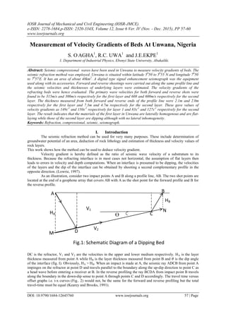
1. IOSR Journal of Mechanical and Civil Engineering (IOSR-JMCE)
e-ISSN: 2278-1684,p-ISSN: 2320-334X, Volume 12, Issue 6 Ver. IV (Nov. - Dec. 2015), PP 57-60
www.iosrjournals.org
DOI: 10.9790/1684-12645760 www.iosrjournals.org 57 | Page
Measurement of Velocity Gradients of Beds At Unwana, Nigeria
S. O.
AGHA1
, R.C. UWA1
and J.E.EKPE1
1. Department of Industrial Physics, Ebonyi State University, Abakaliki.
Abstract: Seismic compressional waves have been used in Unwana to measure velocity gradients of beds. The
seismic refraction method was employed. Unwana is situated within latitude 50
50'
to 50
55'
N and longitude 70
50'
to 70
57'
E. It has an area of about 48km2
. A digital type signal enhancement seismograph was the equipment
used along with its accessories. Forward and reverse shootings were carried out along the same profile line and
the seismic velocities and thicknesses of underlying layers were estimated. The velocity gradients of the
refracting beds were hence evaluated. The primary wave velocities for both forward and reverse shots were
found to be 315m/s and 300m/s respectively for the first layer and 608 and 600m/s respectively for the second
layer. The thickness measured from both forward and reverse ends of the profile line were 2.1m and 2.0m
respectively for the first layer and 7.3m and 4.7m respectively for the second layer. These gave values of
velocity gradients as 149s-1
and 150s-1
respectively for layer 1 and 83s-1
and 127s-1
respectively for the second
layer. The result indicates that the materials of the first layer in Unwana are laterally homogenous and are flat-
laying while those of the second layer are dipping although with no lateral inhomogeneity.
Keywords: Refraction, compressional, seismic, seismograph.
I. Introduction
The seismic refraction method can be used for very many purposes. These include determination of
groundwater potential of an area, deduction of rock lithology and estimation of thickness and velocity values of
rock layers.
This work shows how the method can be used to deduce velocity gradient.
Velocity gradient is hereby defined as the ratio of seismic wave velocity of a substratum to its
thickness. Because the refracting interface is in most cases not horizontal, the assumption of flat layers then
leads to errors in velocity and depth computations. When an interface is presumed to be dipping, the velocities
of the layers and the dip of the interface can be obtained by shooting a second complementary profile in the
opposite direction. (Lowrie, 1997).
As an illustration, consider two impact points A and B along a profile line, AB. The two shot points are
located at the end of a geophone array that covers AB with A as the shot point for the forward profile and B for
the reverse profile.
DC is the refractor, V1 and V2 are the velocities in the upper and lower medium respectively. HA is the layer
thickness measured from point A while HB is the layer thickness measured from point B and 𝜃 is the dip angle
of the interface (fig. I). Obviously, HA > HB. When an impact is made at A, the seismic ray ADCB from point A
impinges on the refractor at point D and travels parallel to the boundary along the up-dip direction to point C as
a head wave before entering a receiver at B. In the reverse profiling the ray BCDA from impact point B travels
along the boundary in the down-dip sense to point A through points C and D accordingly. The travel time versus
offset graphs i.e. t-x curves (Fig.. 2) would not, be the same for the forward and reverse profiling but the total
travel-time must be equal (Kearey and Brooks, 1991).
D
HB
Ө
B
NV1
M
A
HA C
V2
Fig.1: Schematic Diagram of a Dipping Bed

2. Measurement Of Velocity Gradients Of Beds At Unwana, Nigeria
DOI: 10.9790/1684-12645760 www.iosrjournals.org 58 | Page
From the T-X curves, true velocities V1 and V2 of the first and second layers of the subsurface can be obtained
as follows.
𝑉1 =
𝑉𝐼𝐹 + 𝑉𝐼𝑅
2 … … … … … … … … … … . (1)
𝑉2 =
2 cos 𝜃
1
𝑉2𝐹
+
1
𝑉2𝑅
… … … … … … … … … … … … . . …. (2)
where F and R represent forward and reverse profiles respectively and 𝜃 is the dip angle. VIF and VIR
are calculated from the reciprocal slopes, M of the curves. The dip angle 𝜃 and the critical angle, ic are
determined from V1,VIF, and V1R respectively as follows:
𝜃 =
1
2
𝑆𝑖𝑛−1
𝑉1
𝑉1𝐹
+ 𝑠𝑖𝑛−1
𝑉1
𝑉1𝑅
… … … … … … … . . (3)
𝑖 𝐶 =
1
2
𝑆𝑖𝑛−1
𝑉1
𝑉1𝐹
− 𝑠𝑖𝑛−1
𝑉1
𝑉1𝑅
… … … … … … … . . (4)
With the knowledge of the dip angle, 𝜃 the true velocity, V2 is calculated as shown in equation (2) above
(Okwueze, 1988).
Apparent velocities V2F and V2R are obtained from the relations:
1
𝑉2𝐹
=
1
𝑉1
𝑆𝑖𝑛 𝑖 𝑐 + 𝜃 … … … … … … … … … … … . . (5)
1
𝑉2𝑅
=
1
𝑉1
𝑆𝑖𝑛 𝑖 𝑐 − 𝜃 … … … … … … … … … … … . . (6)
The velocity gradient (V/h) at each of the short points for a given layer thickness, h are evaluated using the
values of V1F, V1R, V2F and V2R, etc. This work involves the use of the seismic refraction method to estimate the
velocity gradient at Unwana, Nigeria. Unwana is situated within latitude 50
50'
to 50
55'
N and longitude 70
50'
to
70
55'
E
II. Materials And Method
As in all seismic refraction surveys involving shallow investigations, the materials needed included a
seismograph, sets of geophones, and source of signal. In this particular work, the seismograph was a signal
enhancement type. The geophones were electromagnetic type with frequency 10Hz. The signal was
compressional waves generated mechanically, as a result, only P-wave geophones were arrayed. Single line
𝑀1𝑅 =
1
𝑉1𝑅
TRTF
𝑀2𝑅 =
1
𝑉2𝑅
𝑀𝐼𝐹 =
1
𝑉𝐼𝐹
𝑀2𝐹 =
1
𝑉2𝐹
Distance (x)
Figure 2: T-X curves for forward and reverse
profiles.

3. Measurement Of Velocity Gradients Of Beds At Unwana, Nigeria
DOI: 10.9790/1684-12645760 www.iosrjournals.org 59 | Page
profiling method of seismic refraction survey was adopted. About 12 geophones were interconnected in series
with the shot point and the inter-geophone spacing was 5m. After the initial shooting (forward shooting), the
shot point was moved to the rear of the geophone array for the reverse shot. The shot-detector spacing at both
extremes of the array was also 5m.
III. Result And Discussion
Fig. 4 shows the T-X graph of P-wave data obtained at the study area.
Table 1 shows the velocity gradient (V/h) measured from each end of the shot points for the various layers
delineated by the wave in the study area
Table 1: Velocity (V), thickness (h), and velocity gradient (V/h) obtained in the study area
LAYER FORWARD SHOT REVERSE SHOT
V(m/s) h(m) V/h(s-1
) V(m/s) h(m) V/h(s-1
)
1 314 2.1 140.05 300 2.0 150
2 608 7.3 83.02 600 4.7 127
3 1714 - 1867
IV. Discussion
The T-X graph reveal three geoseismic layers with velocities 314m/s, 608m/s and 1714m/s for layers
1,2 and 3 respectively for the forward shot and velocities 300m/s, 600m/s and 1867m/s for layers 1,2,3
respectively for the reverse shot. These velocities as well as the layer thicknesses, measured from each end of
the profile and the evaluated velocity gradient, are shown in Table I.
Looking at the result, it is seen from Table I that the velocity values for forward and reverse shots which are
314m/s and 300m/s for layer 1 are nearly the same. Their thicknesses also are approximately equal - 2.1m from
the forward shot point and 2.0m from the reverse shot point. The velocity gradients measured are therefore
equal.
However for the second layer, although the seismic velocities measured from both ends of the shot
point are nearly the same (608m/s and 600m/s for forward and reverse shots respectively), the thicknesses at
both ends differ markedly – 7.3m and 4.7m respectively. For this reason, the velocity gradients at both ends of
the shot vary widely – 83.02s-1
and 127s-1
for the forward and reverse ends respectively.
V. Conclusion
The fact that the thickness values of both forward and reverse shots for the first layer are approximately
the same indicates that the interface has negligible dip. The refractor is therefore flat-laying. Again because the
seismic velocities measured from both ends of the profile line are nearly equal implies that lateral differences in
composition of materials are negligible. Thus the materials of the first layer are homogenous and are interpreted
Distance, x (m)
Time,T
(ms)
0 5 10 15 20 25 30 35 40 45
300m/s
588m/s
600m/s
1714m/s1867m/s
313m/s

4. Measurement Of Velocity Gradients Of Beds At Unwana, Nigeria
DOI: 10.9790/1684-12645760 www.iosrjournals.org 60 | Page
to be probably sandy clay. To confirm the absence of dip in the first layer and the homogeneity of materials
there, the velocity gradient has the same value at both ends of the profile line.
However the result for the second layer indicates the presence of dip given the wide variation in thickness at
both ends of the profile line. The material composition nevertheless seems to be uniform throughout the layer as
the seismic velocities are nearly the same at both ends of the profile line. Thus, because of the variation in
thickness, the velocity gradient estimated at both ends of the profile varies widely. The second refractor
therefore is dipping.
References
[1]. Agha, S.O., and Arua, A.I. (2014). Integrated Geophysical Investigation of Sequence of Deposition of Sedimentary Strata in
Abakaliki. European Journal of Physical and Agricultural Sciences. 1(5), 1 – 5.
[2]. Agha, S.O., Okwueze, E.E., and Akpan, T. (2006). Determination of Strength of Foundation Materials in Afikpo, Nigeria, Using
Seismic Refraction Method. Nigerian Journal of Physics. 18(1), 33-37
[3]. Dobrin, M.B. (1976). Introduction to Geophysical Prospecting. McGraw-Hill Book Company Ltd. Japan.
[4]. Kearey, P., and Brooks, M. (1991). An Introduction to Geophysical Exploration(2nd
ed.). Blackwell Scientific Publications,
Cambridge, U.S.A.
[5]. Lowrie, W. (1997). Fundamentals of Geophysics (3rd
Edition). Cambridge University Press, New York.