1. A pluck test was performed on a Cantilever Beam.
To obtain the Acceleration data an IPhone was supported on its edge. Moreover the whole experiment
was captured using an Android phone camera. This was done to perform video analysis using software
called Tracker. Using the tracker two set of values were obtained one is the Acceleration data and the
other is the Amplitude data of vibrations.
This data is then analyzed to calculate the Frequency (F) of Vibrations and the Damping Ratio (Zeta).
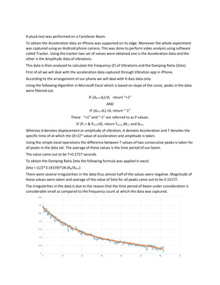
First of all we will deal with the acceleration data captured through Vibration app in iPhone.
According to the arrangement of our phone we will deal with X-Axis data only.
Using the following Algorithm in Microsoft Excel which is based on slope of the curve, peaks in the data
were filtered out.
IF (dX+1-dx)>0, return “+1”
AND
IF (dX+1-dx) <0, return “-1”
These “+1” and “-1” are referred to as P values.
IF (Px > & PX+1<0), return TX+1, dX+1 and AX+1
Whereas d denotes displacement or amplitude of vibration, A denotes Acceleration and T denotes the
specific time of at which the (X+1)th
value of acceleration and amplitude is taken.
Using the simple excel operations the difference between T values of two consecutive peaks is taken for
all peaks in the data set. The average of these values is the time period of our beam.
The value came out to be T=0.2727 seconds
To obtain the Damping Ratio Zeta the following formula was applied in excel.
Zeta = (1/2*3.14159)*LN (AX/AX+1)
There were several Irregularities in the data thus almost half of the values were negative. Magnitude of
these values were taken and average of the value of Zeta for all peaks came out to be 0.15177.
The irregularities in the data is due to the reason that the time period of beam under consideration is
considerable small as compared to the frequency count at which the data was captured.
2. It can be seen that there are several sharp jumps in the data therefore it distorted the value of Damping
Ratio Zeta significantly. To resolve this issue Non-Linear Regression was used to generate an equation.
A=0.2864566-0.01125606*t+0.0002089957*t2
-0.000001539428*t3
Zeta is now calculated for the Acceleration values obtained by the above equation. Which captures the
actual decay in the amplitude of the vibrating beam mass system.
This Zeta came out to be 0.0165
The Excel Solver File provided was also used to calculate Zeta on the same data
The data was divided into three subgroups to check if the zeta is changing with time and amplitude of
vibration. The three time sets are 0-20, 20-40 and 40-60 seconds.
0-20 Seconds
20-40 Seconds
3. 40-60
The video captured through an Android Phone is imported into tracker and using the Auto Track option
Acceleration Data and Amplitude data of vibrations is tracked and imported into Microsoft Excel.
Height of frame was 0.36 meters.
The same Excel operations which were performed on the IPhone data is now performed on Tracker data
and following results were obtained.
4. The regression equation obtained was
Y=3425.498-121.7211*X+1.653022*X2
-0.007769589*X3
The following Values were obtained.
Time Period= 0.273 Seconds
Zeta (Peak Values) = 0.0143
Zeta (Regression Model) = 0.01375
The Data was also then imported into provided Excel Solver file to obtain the results.
It can be observed from the plotted graph that there is a distortion in the acceleration plot this might be
due to the reason that the amplitude is in the direction of gravity therefore the graph is bent more
toward one side of the axis.
The same distortion can be observed in the amplitude data extracted through Tracker. In this case
where amplitude is distorted more on one side of the axis and is almost a flat line on the top. It is not
5. possible to fit a model even for a small time frame. The only solution is the data normalization which will
transfer the amplitude data equally on both side of the horizontal axes.
Several Iterations were performed in Tracker with changed Axis positions and also changing other
parameters in attempt to obtain better quality data but the same pattern was observed.
Summary of Results:
Data Type Time
Period
Frequency Damping
Ratio
(Peaks)
Damping
Ratio
(Regression)
Zeta
0-20 Sec
Zeta
20-40 Sec
Zeta
40-60 Sec
IPhone
Acceleration
0.2727 3.667 0.1517 0.0165 0.001645 0.00154 0.001543
Tracker
Acceleration
0.273 3.663 0.0143 0.01375 - - -
Tracker
Amplitude
- - - - - - -
IPhone data from: Syed Muhammad Raza (101903430)
Video File From: Ali Asad (101900486)
6. A pluck test was performed on a two story sway frame. To capture vibration response of the frame, two
mechanisms were used. First mechanism is that an IPhone was installed on the top of the frame to
capture the vibration data. Second mode of data collection is through video analysis software called
Tracker. The whole experiment was captured using a smart phone and then analyzed to obtain the
vibration data.
Three experiments were performed and the frame was excited in a different mode shape in each
experiment.
In the experiment used in this assignment the bottom storey of the frame was swayed.
Part 1: Tracker Video.
As it can be observed from the image above that both stories of the sway frame were tracked. The
reason to track both stories is to find the mode shapes of the sway frame.
The data extracted from the video is shown in the image below.
The red line represents the displacement of bottom story and the blue line represents the displacement
of top story.
The data is still in raw form and require two operations before further processing. These two operations
are the axis shift and mode decoupling. First of all to identify the modes FFT was performed on the data
and the results were plotted on Y axis with respect to frequency range on X Axis. This gives us frequency
spectrum.
7. Two peaks for each mode was observed and their frequency was noted. Frequency filters were applied
on the FFT results to filter the data. The frequency range applied to filter the first mode is 1-2 Hz and the
frequency range applied to filter second mode is 4-5 Hz. On the filtered data IFFT was performed to get
displacement data according to the desired frequency. It gives us the displacements for the respective
mode shapes.
The first mode plot for top and bottom storey is shown in the picture below.
Blue line represents top story and orange line represents bottom storey.
Similarly the second mode plot for top and bottom story is as follows.
Here the orange line represents the displacement of top story and blue line represent displacement of
bottom storey.
8. The thing to notice here is that it can be observed that the frequency of second mode is several times
more than the first mode. Another important thing to consider is that in the second mode the peak
displacements of first and second story have a phase shift, meaning that they are moving in different
directions at the same time.
To find out the mode shapes 50 consecutive data points for first mode and 25 consecutive data points
for second mode were chosen. The displacement of top story was scaled to unit displacement and the
corresponding displacement of bottom story was calculated. The average values for all the points were
taken and plotted as results.
The following mode shape was obtained from the above mentioned analysis for first mode. Similarly for
second mode.
The following mode shape was obtained for the second mode after performing the analysis.
9. To calculate the frequency and damping ratio the least square curve fit method is to be used.
The calculations for first mode is shown in the image below.
Calculations for the second mode is shown in the picture below.
Part B: IPhone Data Analysis
The plot of the data obtained through Vibration app in IPhone is displayed in the picture below.
Similarly the frequency data was also plotted.
10. The modes were then decoupled according to their frequency ranges. For this operation the same
procedure was followed as observed in the tracker app data analysis. Amplitudes of decoupled modes
are plotted in the image below.
To find out the FREQUENCY damping characteristics of the two modes Least Squares Curve Fit Method is
used. The results obtained for the first mode is shown in the image below.
11. Similarly for the second mode.
To calculate the mode shape from IPhone data we have to use analytical formulas for these we use the
frequency values calculated above.
The relevant calculations for the mode shape calculation are show in hand calculations at the end of the
assignment.
To find out the modal ratio five peaks were taken from the first mode data and five peaks from second
mode of IPhone data. Average value of these peaks for each mode were calculated and their ratio was
taken which came out to be 12.957. The same procedure was followed on Tracker data and modal ratio
was calculated which came out to be 7.253. The reason of this difference can be attribute to the
difference in the frequency of data counts per second. For iPhone frequency of data is 64 Hz and for
Tracker the data had 30 frames per second.
The first mode is at least 7 time more dominant then the second mode this can be attribute to the
nature of the pluck test. In first mode the stories are displaced in the same direction at the same time as
was the nature of our initial push. So the first mode came out to be dominant as compared to the
second mode in which the stories move in different directions at the same time.
Part 3: Eigen Value Analysis:
Now input the Values calculated from the static experiments in the Eigen Value Analysis Excel Sheet file.
The relevant calculations are shown on the attached papers on the end of assignment. The following
results were obtained from the calculations.
12. The results of the experiment is summarized as follows.
Summary
First Mode Second Mode
Frequency Damping
Ratio
Frequency Damping
Ratio
Vibration
Data
1.380 0.01024 4.405 0.005849
Tracker
Data
1.370 0.01019 4.366 0.006462
Eigen Value
Analysis
2.14 - 5.46 -