http://iosrjournals.org/iosr-jeee/pages/v6i3.html

1. IOSR Journal of Electrical and Electronics Engineering (IOSR-JEEE)
e-ISSN: 2278-1676,p-ISSN: 2320-3331,Volume 6, Issue 3 (May. - Jun. 2013), PP 82-90
www.iosrjournals.org
www.iosrjournals.org 82 | Page
Effects of Weight Approximation Methods on Performance of
Digital Beamforming Using Least Mean Squares Algorithm
Pranav Wani1
, Amalendu Patnaik2
1
B.Tech Student, IIT Roorkee, India
2
Assistant Professor, IIT Roorkee, India
Abstract : Adaptive Arrays are currently the subject of extensive research, for improving the quality of the
receiving signals in the presence of interfering signals in wireless communications. In this paper
beamforming is performed considering a digital system using Least Mean Squares algorithm. The main
emphasis is to discuss the effects of the weight approximation procedures on the overall performance of the
LMS algorithm and the Beamforming. The same results can be obtained for other adaptive beamforming
algorithms and their various modifications available in the literature. In this paper Least Mean Squares
Algorithm has been used to show the effects of weight approximation methods. Weight approximation methods
are used to convert the continuous valued weights into discrete valued weights which can be used by digital
systems for beamforming. Two algorithms have been proposed for weight approximation. Their performance
has been compared with the conventional methods. Comparisons have been made for Beampattern, Sidelobe
level, Convergence rate, Stability. The proposed algorithms have been observed to give overall better results
for slight increase in the computational cost. The effect of the convergence coefficient 𝞵 on the sidelobe levels
of beampattern has also been discussed.
Keywords – Digital Beamforming, Least Mean Squares Algorithm, Phased Array Antenna, Weight
Approximation
I. INTRODUCTION
An adaptive array [1] can be best described as a collection of sensors, feeding a weighting and
summing network, with automatic signal dependent weight adjustments to emphasis the desired signal. With the
direction of the incoming signals known or estimated, the next step is to use spatial processing techniques to
improve the reception performance of the receiving antenna array based on this information. Some of these
spatial processing techniques to improve the SNR are referred to as beamforming. Given a one dimensional
linear array of elements and an impinging wavefront from an arbitrary point source, the directional power
pattern P(Ѳ) can be expressed as
𝑃 Ѳ = 𝑎 𝑥 𝑒−𝑗𝛽𝑑 𝑥,Ѳ
𝑑𝑥
Where a(x) is the amplitude distribution along the array, B is the phase constant, and d(x, Ѳ) is the
relative distance the impinging wavefront, with an angle of arrival theta, has to travel between points uniformly
spaced a distance x apart along the length of the array.
There are several beamforming techniques available such as LMS, RMS, MVDR Beamforming,
Classical Beamformer etc [1]. With the advancement in the integrated digital systems, formation of beam is
being controlled by digital systems. Thus the selection of magnitude and phase of weights are being controlled
by digital systems. Digital systems have many benefits, most significantly the small space requirements, low
cost, very high speed. Thus in the backdrop of this it becomes important to investigate the various factors that
control the digital beamforming.
The main focus of this paper is to investigate the methods of converting the continuous weights to
discrete weights which can be used by digital systems.
II. Least Mean Squares Algorithm
2.1 Introduction
If sufficient knowledge of the desired signal is available, a reference signal d can then be generated.
These reference signals are used to determine the optimal weight vector wMSE=[W1, W2, ………. , Wn]. This is
done by minimizing the mean square error of the reference signals and the output of the N-element antenna
array.
The concept of reference signal use in adaptive antenna system was first introduced by Widrow where
he described several pilot-signal generation techniques. One of the proposed techniques was a two mode
adaption process whereby the transmitter alternated between sending a known pilot signal and actual data. The
receiver had the knowledge of the pilot signal and used it as the desired response for the LMS adaptive

2. Effects of Weight Approximation Methods On Performance of Digital Beamforming Using Least
www.iosrjournals.org 83 | Page
algorithm. During actual data transmission, adaption would be switched off and the weights would coast until
the pilot signal was turned back on. While this technique was never actually constructed, it provided the
necessary impetus.
For beamforming considerations, the reference signal is usually obtained by a periodic transmission
of a training sequence, which is a priori known at the receiver and is referred to as temporal reference.
Information about the direction of the signal of interest is usually referred to as spatial reference.
The LMS algorithm [1] is probably the most widely used adaptive filtering algorithm, being
employed in several communication systems. It has gained popularity due to it’s low computational complexity
and proven robustness. It incorporates new observations and iteratively minimizes linearly the mean square
error. The LMS[1] algorithm changes the weight vector w along the direction of the estimated gradient based on
the negative steepest descent method. By the quadratic characteristics of the mean square error function that has
only one minimum, the steepest descent is guaranteed to converge. The LMS [1] algorithm updates the weight
vector according to
𝑤 𝑘 + 1 = 𝑤 𝑘 −
𝜇
2
𝜕𝐽 𝑤,𝑤 ∗
𝜕𝐽 𝑤 ∗
= 𝑤 𝑘 + 𝜇𝑒∗
𝑘 𝑥(𝑘)
Where, the rate of change of the objective function Jw,w’=|e(k)|^2 has been derived earlier in and 𝞵
is a scalar constant which controls the rate of convergence and stability of the algorithm. In order to guarantee
stability in the mean-squared sense, the step size 𝞵 should be restricted in the interval
0 < 𝜇 < 2/𝜆 𝑚𝑎𝑥
𝜆 𝑚𝑎𝑥 ≤ 𝑡𝑟𝑎𝑐𝑒{𝑅 𝑥𝑥 }
0 < 𝜇 <
2
𝐸{𝑥𝑖
2
}𝑁
𝑖=1
Here N is the number of elements in the array. 𝞵 is the convergence coefficient. It determines the
convergence and stability of beampattern of the antenna. The algorithm can be stated as:
𝑒 𝑘 = 𝑑 𝑘 − 𝑤 𝐻
𝑘 𝑥 𝑘
𝑤 𝑘 + 1 = 𝑤 𝑘 + 𝜇𝑒∗
𝑘 𝑥 𝑘
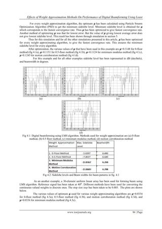
Beampattern of a 6-element linear array using LMS algorithm is shown below. The beam has been formed at
400
.
Fig 2.1: Beamforming using recursive Least Mean Squares algorithm for a 6-element uniform linear array.
Reference signal is at 400
2.2 Digital Beamforming using LMS Algorithm
While forming the beampattern using LMS algorithm, the weights are iteratively updated. The
magnitude and the phase of the weights are provided to the antenna elements using analog systems. With the
advances in the integrated digital systems, it has become more convenient to provide the required magnitude and
phase to the elements digitally. Since there exists a limitation to the values that can be provided using digital
systems, it becomes important to study the methods to convert the analog values to the digital values so as to
obtain the acceptable output of the antennas. In this report two available methods for the conversion of
contentious values to discrete values have been mentioned. Further two new methods have been suggested. It

3. Effects of Weight Approximation Methods On Performance of Digital Beamforming Using Least
www.iosrjournals.org 84 | Page
has been observed that the two new methods provide significant improvement over the available methods in
terms of antenna beampattern, sidelobe levels and small improvement over convergence rate.
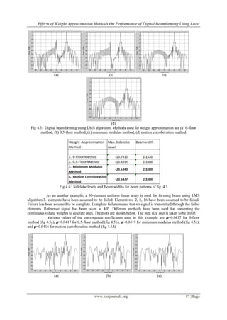
2.3 Importance of Convergence Coefficient
LMS algorithm depends on the continuous upgradation of the weights to get the desired beam in a
particular direction. The convergence rate of the algorithm depends on the convergence coefficient 𝞵. Larger
coefficient ensures larger steps, but it comes at the cost of stability. Smaller coefficients make the step size
smaller, but the deviation is also small, which compensates for the small step size. Thus too large or too small 𝞵
tends to give slow convergence. There is a optimum value of 𝞵 which provides the fastest convergence.
Thus the maximum convergence rate is obtained at a particular optimum value of 𝞵. This optimum
value depends on
-> The design of the array
-> The environmental condition
(Environmental conditions include the noise present in the environment.)
To illustrate the effect of convergence coefficient 𝞵 on the convergence rate a 6-element uniform
linear array has been considered. Beam has been formed using LMS algorithm. Error plots are shown below for
three values of 𝞵; 0.1, 0.2, and 0.3.
Fig 2.2: Error plots for different values of 𝞵 using Least Mean Squares Algorithm
III. Conversion Of Analogous Weights To Digital Weights
3.1 Conventional Algorithms to convert Continuous Valued Weights to Discrete Valued
Weights
a)0-Floor Method
This method is most basic way to determine the value of any number available in continuous scale
for the use in digital systems, and is widely used [2]. In this method the number is approximated to the nearest
available number to the left of it. Continuous weights are converted to discrete values by shifting the decimal
numbers to the nearest left integer. The LMS algorithm can thus be written as:
𝑒 𝑘 = 𝑑 𝑘 − 𝑤 𝐻
𝑘 𝑥 𝑘
𝑤 𝑘 + 1 = 𝑤 𝑘 + 𝜇𝑒∗
𝑘 𝑥 𝑘
𝑓 = 𝑓𝑙𝑜𝑜𝑟[
𝑤 𝑘 + 1
𝑠𝑡𝑒𝑝
]
𝑤(𝑘 + 1) = 𝑓 ∗ 𝑠𝑡𝑒𝑝
Here ‘w’ is the value of weight in continuous scale. ‘Step’ is the step size of the available digital
system. It is the minimum distance between two nearest numbers that the system can provide. Step is the
resolution of the digital system.
b)0.5-Floor Method
This method is another available method to convert the analog values to the digital [2]. In this
method the number is approximated to the nearest available value. It may thus be shifted either to the left or

4. Effects of Weight Approximation Methods On Performance of Digital Beamforming Using Least
www.iosrjournals.org 85 | Page
right depending upon it’s location between the two nearest available values. The LMS algorithm can thus be
given as: step is the step size.
𝑒 𝑘 = 𝑑 𝑘 − 𝑤 𝐻
𝑘 𝑥 𝑘
𝑤 𝑘 + 1 = 𝑤 𝑘 + 𝜇𝑒∗
𝑘 𝑥 𝑘
𝑤(𝑘 + 1) = 𝑤(𝑘 + 1) +
𝑠𝑡𝑒𝑝
2
𝑓 = 𝑓𝑙𝑜𝑜𝑟
𝑤(𝑘 + 1)
𝑠𝑡𝑒𝑝
𝑤(𝑘 + 1) = 𝑓 ∗ 𝑠𝑡𝑒𝑝
3.2 Improved Algorithms for converting Continuous valued Weights into Discrete Valued
Weights
a)Minimum Modulus Method
This is one of the two methods that have been proposed. After simulations it can be observed that
this method provides better results compared to the available methods.
In this method the value of the weights are selected to the nearest value available in the left or in the
right on the number line depending on the value of the modulus of the output. Thus a decimal number would be
shifted to the nearest value available in the left if the number if positive. Similarly, a number would be shifted to
the nearest value available in the right of the number scale, if the number is negative.
Thus the LMS algorithm can be written as:
𝑒 𝑘 = 𝑑 𝑘 − 𝑤 𝐻
𝑘 𝑥 𝑘
𝑤 𝑘 + 1 = 𝑤 𝑘 + 𝜇𝑒∗
𝑘 𝑥 𝑘
𝑤(𝑘 + 1) = 𝑤(𝑘 + 1) ; 𝑖𝑓 𝑤 ≥ 0
𝑤(𝑘 + 1) = 𝑤(𝑘 + 1) + 𝑠𝑡𝑒𝑝 ; 𝑖𝑓 𝑤 < 0
𝑓 = 𝑓𝑙𝑜𝑜𝑟[
𝑤(𝑘 + 1)
𝑠𝑡𝑒𝑝
]
𝑤(𝑘 + 1) = 𝑓 ∗ 𝑓𝑙𝑜𝑜𝑟
b)Motion Corroboration Method
In this method the value of the weights is approximated depending on the present value of the
weights as well as the previous values of the weights. The values are approximated so as to corroborate the
direction of motion of the weights. Thus if a number in the present iteration has shifted right with respect to it’s
position in previous iteration, then the number will be approximated to it’s nearest value available in the right.
Similarly, if a number has shifted left in it’s present iteration compared to it’s position in the previous iteration,
then the number will be approximated to the nearest available value to it’s left.
Thus the LMS algorithm using motion corroboration algorithm for weight approximation can be
written as: step is the step size, and e is the error.
𝑒 𝑘 = 𝑑 𝑘 − 𝑤 𝐻
𝑘 𝑥 𝑘
𝑤 𝑘 + 1 = 𝑤 𝑘 + 𝜇𝑒∗
𝑘 𝑥 𝑘
𝑤(𝑘 + 1) = 𝑤(𝑘 + 1) + 𝑠𝑡𝑒𝑝 ; 𝑖𝑓 𝑒 ≥ 0
𝑤(𝑘 + 1) = 𝑤(𝑘 + 1) ; 𝑖𝑓 𝑒 < 0
𝑓 = 𝑓𝑙𝑜𝑜𝑟
𝑤(𝑘 + 1)
𝑠𝑡𝑒𝑝
𝑤(𝑘 + 1) = 𝑓 ∗ 𝑠𝑡𝑒𝑝
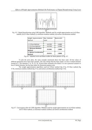
IV. Experimental Simulations
We have used a 10-element linear array. Beam has been formed using Least Mean Squares algorithm.
The reference signal has been taken at 400
. The step size ‘step’ used is 0.01. For weight approximation, above
discussed four algorithms have been used.

5. Effects of Weight Approximation Methods On Performance of Digital Beamforming Using Least
www.iosrjournals.org 86 | Page
For every weight approximation algorithm, the optimum 𝞵 has been calculated using Particle Swarm
Optimization Algorithm (PSO) to get the minimum sidelobe level. Minimum sidelobe level is obtained for 𝞵
which corresponds to the fastest convergence rate. Thus 𝞵 has been optimized to give fastest convergence rate.
Another method of optimizing 𝞵 was that for lowest error. But the value of 𝞵 giving lowest average error does
not give lowest sidelobe level. This result has been shown through simulation in section 5.
Thus for this simulation and for all the other simulations presented in this article, 𝞵 has been optimized
for every weight approximating algorithm, to give the fastest convergence rate. This ensures the minimum
sidelobe level for every algorithm.
After optimization, the various values of 𝞵 that have been used in this example are 𝞵=0.1148 for 0-floor
method (fig 4.1a), 𝞵=0.1151 for 0.5-floor method (fig 4.1b), 𝞵=0.1124 for minimum modulus method (fig 4.1c),
𝞵=0.1245 for motion corroboration method (fig 4.1d).
For this example and for all other examples sidelobe level has been represented in dB (decibels),
and beamwidth in degrees.
(a) (b) (c)
(d)
Fig 4.1: Digital beamforming using LMS algorithm. Methods used for weight approximation are (a) 0-floor
method, (b) 0.5 floor method, (c) minimum modulus method, (d) motion corroboration method
Fig 4.2: Sidelobe levels and Beam widths for beam patterns in fig. 4.1
As an another example, a 30-element uniform linear array has been used for forming beam using
LMS algorithm. Reference signal has been taken at 400
. Different methods have been used for converting the
continuous valued weights to discrete ones. The step size step has been taken to be 0.005. The plots are shown
below.
The various values of optimum 𝞵 used for various weight approximating algorithms are 𝞵=0.0334
for 0-floor method (fig 4.3a), 0.5-floor method (fig 4.3b), and motion corroboration method (fig 4.3d), and
𝞵=0.0336 for minimum modulus method (fig 4.3c).

6. Effects of Weight Approximation Methods On Performance of Digital Beamforming Using Least
www.iosrjournals.org 87 | Page
(a) (b) (c)
(d)
Fig 4.3: Digital beamforming using LMS algorithm. Methods used for weight approximation are (a) 0-floor
method, (b) 0.5-floor method, (c) minimum modulus method, (d) motion corroboration method
Fig 4.4: Sidelobe levels and Beam widths for beam patterns of fig. 4.3
As an another example, a 30-element uniform linear array is used for forming beam using LMS
algorithm.3- elements have been assumed to be failed. Element no. 2, 8, 16 have been assumed to be failed.
Failure has been assumed to be complete. Complete failure means that no signal is transmitted through the failed
elements. Reference signal has been taken at 400
. Different methods have been used for converting the
continuous valued weights to discrete ones. The plots are shown below. The step size step is taken to be 0.005.
Various values of the convergence coefficients used in this example are 𝞵=0.0417 for 0-floor
method (fig 4.5a), 𝞵=0.0417 for 0.5-floor method (fig 4.5b), 𝞵=0.0419 for minimum modulus method (fig 4.5c),
and 𝞵=0.0416 for motion corroboration method (fig 4.5d).
(a) (b) (c)

7. Effects of Weight Approximation Methods On Performance of Digital Beamforming Using Least
www.iosrjournals.org 88 | Page
(d)
Fig 4.5: Digital beamforming using LMS algorithm. Methods used for weight approximation are (a) 0-floor
method, (b) 0.5-floor method, (c) minimum modulus method, (d) motion corroboration method
Fig 4.6: Sidelobe levels and Beam widths for beam patterns of fig. 4.5
To plot the error plots, the same example mentioned above has been used. All the values of
different parameters have been kept constant. The only change that has been made is to have 6 failed elements
instead of 3. The elements 2, 8, 16, 22, 26, 30 have been assumed to be failed. It is not a practical scenario to
have 6 failed elements, but has been taken for illustration purpose only.
The weight approximation algorithms used are 0-floor method (fig 4.7a), 0.5-floor method (fig
4.7b), minimum modulus method (fig 4.7c), and motion corroboration method (fig 4.7d).
(a) (b) (c)
(d)
Fig 4.7: Convergence plots for LMS algorithm. Methods used for weight approximation are (a) 0-floor method,
(b) 0.5-floor method, (c) minimum modulus method, (d) motion corroboration method

8. Effects of Weight Approximation Methods On Performance of Digital Beamforming Using Least
www.iosrjournals.org 89 | Page
Fig 4.8: Sidelobe levels and Beam widths for convergence plots of fig. 4.7
From the above examples it can be observed that the two proposed algorithms, Minimum Modulus
method and Motion Corroboration method perform significantly better that the 0-floor method and 0.5-floor
method in terms of sidelobe level. The sidelobe levels obtained by the proposed methods are significantly lower
for a small increment in the beamwidth, and computational cost.
The convergence rate of LMS algorithm using motion corroboration is the fastest among the four
discussed algorithms. It can also be observed that the output of LMS using minimum variance method is the
most stable.
V. Efect Of Convergence Coefficient 𝞵
In this section, we wish to find the optimum value of convergence coefficient 𝞵 to get the lowest
sidelobe levels using Least Mean Squares Algorithm. Here we are using digital beamformer. For the purpose of
weight approximation we use motion corroboration algorithm.
For the purpose of simulation, a 6- element uniform linear array has been used. The step size step
has been fixed to 0.1. The reference signal is assumed to be at 400
. We have used five different values of 𝞵. One
of the values of 𝞵 has been calculated by PSO for the condition of fastest convergence rate. The value of 𝞵
found for fastest convergence rate was 𝞵=0.1423. Another value of 𝞵 was calculated using PSO for the
condition of lowest steady state error. The value of 𝞵 for lowest steady state error was found to be 𝞵=0.050. The
remaining three values were randomly taken to be in the vicinity of the two calculated values. The other three
values of 𝞵 that were used are 𝞵=0.0213, 0.00803, 0.0617.
The error plots for the two calculated values, fastest convergence rate (0.1423), and lowest steady
state error (0.050) are shown in fig 5.1. The beam patterns using all the five values of 𝞵 are shown in fig 5.2.
Fig 5.1: Convergence plot for LMS algorithm using motion corroboration method for weight approximation for
two values of 𝞵 (0.050, and 0.1423)

9. Effects of Weight Approximation Methods On Performance of Digital Beamforming Using Least
www.iosrjournals.org 90 | Page
Fig 5.2: Digital Beamforming using LMS algorithm with motion corroboration as weight selection algorithm.
Fig 5.3: Sidelobe levels and Beam widths for beam patterns of fig. 5.2
From the above plots it can be clearly seen that the lowest sidelobe levels is obtained in LMS
algorithm for the value of 𝞵 that corresponds to the fastest convergence rate. Thus it can be concluded that the
value of 𝞵 corresponding to the fastest convergence rate, and not the one corresponding to the lowest steady-
state error, results in the lowest sidelobe levels.
VI. Conclusion
In this article digital beamforming using Least Mean Squares algorithm was discussed. The focus of
this article was to discuss the effects of weight approximation algorithms on the beamforming algorithms.
Approximately the same effects can be observed with various beamforming algorithms and their derivatives
available in the literature. However in this article only basic LMS algorithm was considered.
In this article two new weight approximation methods were proposed. It was observed that the
performance of the proposed algorithms were better than the available methods. The new proposed methods
resulted in the significantly lower sidelobe levels and faster convergence rate at the rate of small increase in
computational cost. In this article it was also shown that the lowest sidelobe levels are obtained for 𝞵
corresponding to the fastest convergence rate and not necessarily to the 𝞵 corresponding to the lowest steady-
state error.
REFERENCES
[1] Constantine A. Balanis and Panayiotis I. Ioannides, Introduction to Smart Antennas, 1st
edition: Morgan & Claypool, 2007
[2] Donald Hearn and M. Pauline Baker, Computer Graphics – C Version, Prentice Hall of India.
[3] J. Kennedy and R. C. Eberhart, Swarm Intelligence, San Francisco, CA: Morgan Haufmann, 2001