1. As bean beetle embryos develop, time-lapse photographs of their eggs exhibit varying levels of brightness that correspond to different stages of maturation. These time
signals can be analyzed to pinpoint when different stages of development occur. These stages are marked by transitions in the time signal, for which we have developed
a method to accurately identify and predict. Wavelet transforms are utilized to analyze the signal over various time windows in order to identify features of varying
scales within the signal. Key features are then extracted from the wavelet analysis in order to use as inputs to a neural network, which will automate the process of
identifying and predicting the points of transition. We have studied this method’s accuracy at various levels of noise using simulated data based off lab data.
Abstract
Zachary Diener
Dr. Paul Pearson
Department of Mathematics
Hope College, Holland, MI 49423
Motivation
Bean beetles are an invasive agricultural pest native to Africa and Asia that
cause a great deal of damage to crops each year. Due to their short life span
and ease of care they are a model organism to study. This project focused on
using these beetles to test the practically of making time-frequency
predictions using neural networks which can then be expanded to study a
wider variety of pests in order to mitigate their damaging effects.
Artificial Neural Networks
Artificial neural networks are statistical learning models used in machine learning that make calculated
predictions of an output based on multiple inputs. These functions are modeled after the connections in the brain
and operate in a similar way. Rather than consisting of synapses and neurons, artificial neural networks consist of
3 parts. Those would be an Input Layer, Hidden Layer and Output Layer; all of which are connected through sets
of activation functions and weights. The network learns by changing weights through the optimization of a cost
function which analyzes the cost of making certain predictions on a set of training data where the desired output is
known. To prepare the time signals to be inputted into the neural network, time signals were processed using the
modified Haar Wavelet Transform, then key features were selected using the Kirsch 5 x 5 Edge Detector. This
resulted in an output matrix of dimension 70 x 1 which was then input into the neural network. This process was
repeated for all of the 330 simulation time signals. 200 of these signals were used as training data, thus the
network was told where the transition points should occur in each individual signal. The remaining 130 signals
were then used to test the accuracy of the networks predictions. For these signals the network was presented with
the input variables however the time at which the transition points occur was now withheld. The resulting
predictions were then compared with the expected values to determine the networks accuracy.
Heatmap Construction
Once an array of differences or wavelet scaling coefficients has been constructed, these extracted coefficients are plotted in
heatmap. These heatmap plots allow for the visualization of features across the various frequency levels extracted in the wavelet
transform. In the images below, a section of the scaling coefficients array is shown, along with the corresponding heatmap. The
darker regions of the heatmap correspond to large changes in the time signal while lighter regions indicate less change in the
signal. The uppermost row contains the highest frequency data while the lowest row contains the low frequency data. It is
apparent that the most significant features of the time signal occur after the 45th time unit.
Time
…
…
…
…
…
…
…
…
…
…
Heatmap of Haar Wavelet Transform Wavelet Scaling Coefficients Array
Conclusions and Future Work
The data chosen for this project, although synthetic, is essentially real laboratory data
with noise and time lags added, so the results of our research should generalize well to
real-world data. We found that using wavelet transforms to process signals in preparation
to utilize neural networks to make time-frequency predictions resulted in accurate
predictions of key points in a time signal. In the future we will continue to explore
various edge detectors and their effect on the the predictions of the neural network. We
would also like to explore various neural networks and their resulting prediction accuracy.
Kirsch Edge Detector
Acknowledgements
• Dr. Paul Pearson
• Dr. Brian Yurk
• David McMorris
• Nyenhuis Grant
• Hope College Mathematics
Department
Modified Haar Wavelet Transform
Wavelets are commonly utilized in signal processing for their ability to detect sudden changes in the signal. Wavelets express a
signal as a sum of smaller component waves of a fixed frequency. These component waves are calculated from a time dilated and
amplitude scaled “mother wavelet” and can extract data from various frequency levels. To process our signal a modified form of
the Haar Wavelet Transform was employed. Starting with the original time signal, an array of averages was calculated using a
sliding window of various frequencies. From here an array of the differences between the averages of various frequencies was
constructed. These differences correspond to the scaling coefficients used to translate the mother wavelet into the extracted
wavelets. These averages and differences can be described by the following functions when j ≥ 1, where j corresponds to the row
index and n corresponds to the column index.
Although it is not easily visually interpreted, the differences array contains the data which will exemplify the features of the time
signal. To reduce noise a soft threshold was applied to the array. This process takes values above the threshold and reduces them
by the threshold value. Values below the the negative of the threshold are increased by the threshold values. Finally values
between the threshold and its negative are set to zero. This process decreases the range of the data and removes a majority of the
Gaussian white noise.
Results
Using the Kirsch 5 x 5 Edge Detector and a neural network of 70 input variables and 30 hidden
variables we were able to on average predict the transition period within a window of 13.7 minutes.
Each signal was approximately 24 hours long and had varied amounts of injected noise. Our
network made very accurate predictions on all but the nosiest of signals. Below are the differences
between the expected and predicted values along with the corresponding noise of the signal.
Once the signal had been processed using the wavelet transforms and then plotted with the heatmap, it was
decided to select key features of the data in order to reduce the time needed to train the neural network. This
feature selection was done with the Kirsch Edge Detector. Using the Kirsch Filter matrix, which is rotated by 45
degrees to obtain the eight various filters, this method of feature selection rewards edges going in certain directions
and penalizes edges in other directions, depending on which filter is used. These filters select sections of the data
matrix, then both the filter and the selected data is flattened and the dot product of the two is calculated. This dot
product is then placed in the center of the the selected are of data. This process is then repeated as the filter slides
along the data matrix until reaching the end. The resulting output is a new data matrix in which the edges are are
more pronounced.