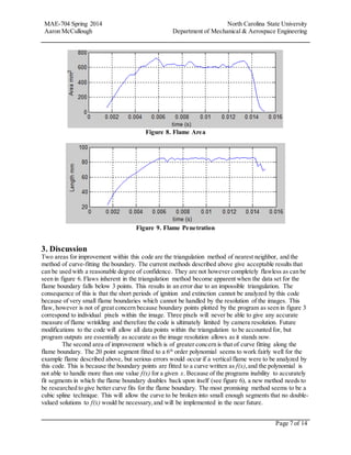
This document describes an image analysis program that analyzes high-speed camera images of turbulent flames. The program takes flame image files as input and generates a probability density function of radii of curvature along the flame boundary contour. It also tracks flame area and penetration over time. Key steps include thresholding images, finding boundary points, connecting points using Delaunay triangulation and nearest neighbors, fitting polynomials to contour segments, and calculating radii of curvature along the contour.

1. College of Engineering
Department of Mechanical and Aerospace Engineering
MAE-704
Fluid Dynamics of Combustion II
Image Analysis of Turbulent Flame Tomography
Aaron McCullough

2. MAE-704 Spring 2014 North Carolina State University
Aaron McCullough Department of Mechanical & Aerospace Engineering
Page 2 of 14
Abstract
A program for the analysis of turbulent flame images is presented. Flame image files are
accepted as inputs, and a contour of each flame boundary is then generated to produce a
probability density function of radii of curvature along the contour. Once this has been achieved,
turbulent scales responsible for flame shape can be ascertained based on flame geometry.
Secondary outputs are flame area and flame penetration as a function of flame lifetime. The code
is demonstrated to be a useful tool for post-processing of high-speed camera imaging, and areas
of improvement and further study are presented.

3. MAE-704 Spring 2014 North Carolina State University
Aaron McCullough Department of Mechanical & Aerospace Engineering
Page 3 of 14
1. Introduction
High speed photography is one of the most widely used experimental tools for combustion
research. One area of particular interest in which this tool is utilized is that of turbulent flame
imaging. Most scholarly articles on this topic deal with laser diagnostic techniques of flame
experimentation, but the specific area to which this project seeks to contribute is that of turbulent
flame tomography. Reference [1] provides an excellent example of what is being done in this
field today. In that particular study, flame images were converted to binary images and Fourier
transformations were used to determine flame curvature distribution. The method presented in
the following pages takes a more visual approach by directly analyzing turbulent flame images.
Once image data is obtained, the necessity arises for programming aids which can quickly
analyze flame images and output parameters and graphical data to describe the nature of the
flame. One such code has been developed by the author to achieve this goal, and the methods
employed in its development, and the resulting output are the subject of this report. Given a set
of frames from a high speed video of a turbulent flame in a combustion chamber, the primary
objective of this program is to determine the degree of wrinkling of the flame by generating a
probability density function of radius of curvature along the flame boundary. A secondary
objective is to track the flame area and flame penetration into the chamber over flame lifetime.
The code was written in MATLAB and is found in the appendix, however the following methods
will describe the approach used in analyzing images rather than detailing MATLAB specific
functions.
2. Methods
A Diesel flame was ignited in a combustion chamber with the following ambient conditions -
temperature of 1000 Kelvin, pressure of 44 Barr,density of 15 kg per cubic m, and 21% oxygen by
volume. The flame was photographed with a high speed camera at a rate of 4500 frames per second. The
resulting 400 x 128 pixel images were converted to .png files and were read into the program in this
format - shown below in figure 1. Using a reference image with a grid of known dimensions, it was
determined that there were approximately 35 mm per 148 pixels or .23 square mm per pixel.
Figure 1. Flame Image
The first step in image analysis is to determine the boundary points of the flame. Each pixel has a
grayscale value between 0 and 255. It has been determined that the best results come from setting the
threshold value at 40. The image is then scanned by the program and all pixels below 40 are set to zero,
and all above 40 are set to 200. This scan results in a matrix whose corresponding image is shown below
in figure 2.

4. MAE-704 Spring 2014 North Carolina State University
Aaron McCullough Department of Mechanical & Aerospace Engineering
Page 4 of 14
Figure 2. Flame Threshold
The next step in processing is to scan this image for boundary points. The condition for a boundary point
is a value of 200 at the point and at least one value of zero in the 4 locations adjacent to it. At this point in
the program, the boundary is also converted from pixel location to realx and y values in mm. The
resulting code generates x and y vectors which have been plotted in the image shown in figure 3.
Figure 3. Flame Boundary Points
Once these boundary points have been determined, they must be connected by a smooth contour. This
step represents the most challenging part of the program because an algorithm must be employed to sort
each boundary point based on which point is nearest to it. It has been ultimately discovered that a
Delaunay triangulation of the plot is needed to determine each point’s nearest neighbor. A description of
Delaunay triangulation is described in reference [2] and the nearest neighbor technique can be found in
reference [3]. Figure 4 shows the Delaunay triangulation of the example image.
Figure 4. Delaunay Triangulation
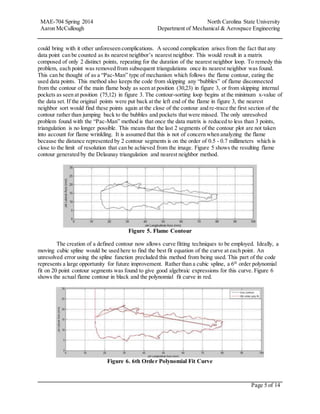
There are severalcomplications that must be dealt with when using this technique. The first is caused by
the nearest neighbor function. If the point of interest is used as the query point, it must be taken out of the
triangulation, or else it will be counted as its own nearest neighbor. For this reason,the code removes
each point from the data before performing a triangulation. It then inserts the point as a query point to find
its respective nearest neighbor. This complication could possibly be resolved by using a function which
finds the 2nd
nearest neighbor to a point included within the triangulation. Such a function was not
researched because the method described above was found to work well, and because such a function

5. MAE-704 Spring 2014 North Carolina State University
Aaron McCullough Department of Mechanical & Aerospace Engineering
Page 5 of 14
could bring with it other unforeseen complications. A second complication arises from the fact that any
data point can be counted as its nearest neighbor’s nearest neighbor. This would result in a matrix
composed of only 2 distinct points, repeating for the duration of the nearest neighbor loop. To remedy this
problem, each point was removed from subsequent triangulations once its nearest neighbor was found.
This can be thought of as a “Pac-Man” type of mechanism which follows the flame contour, eating the
used data points. This method also keeps the code from skipping any “bubbles” of flame disconnected
from the contour of the main flame body as seen at position (30,23) in figure 3, or from skipping internal
pockets as seen at position (75,12) in figure 3. The contour-sorting loop begins at the minimum x-value of
the data set. If the original points were put back at the left end of the flame in figure 3, the nearest
neighbor sort would find these points again at the close of the contour and re-trace the first section of the
contour rather than jumping back to the bubbles and pockets that were missed. The only unresolved
problem found with the “Pac-Man” method is that once the data matrix is reduced to less than 3 points,
triangulation is no longer possible. This means that the last 2 segments of the contour plot are not taken
into account for flame wrinkling. It is assumed that this is not of concern when analyzing the flame
because the distance represented by 2 contour segments is on the order of 0.5 - 0.7 millimeters which is
close to the limit of resolution that can be achieved from the image. Figure 5 shows the resulting flame
contour generated by the Delaunay triangulation and nearest neighbor method.
Figure 5. Flame Contour
The creation of a defined contour now allows curve fitting techniques to be employed. Ideally, a
moving cubic spline would be used here to find the best fit equation of the curve at each point. An
unresolved error using the spline function precluded this method from being used. This part of the code
represents a large opportunity for future improvement. Rather than a cubic spline, a 6th
order polynomial
fit on 20 point contour segments was found to give good algebraic expressions for this curve. Figure 6
shows the actual flame contour in black and the polynomial fit curve in red.
Figure 6. 6th Order Polynomial Fit Curve

6. MAE-704 Spring 2014 North Carolina State University
Aaron McCullough Department of Mechanical & Aerospace Engineering
Page 6 of 14
It can be seen in figure 6 that the polynomial fit has the most difficulty in areas where the contour doubles
back on itself and in regions of infinite slope. These areas specifically are examples of where a spline fit
would be more accurate. Other than these few discrepancies between the true contour and the polynomial
fit, the above figure shows a reasonably accurate algebraic representation of the flame boundary. Other
images within the video were also found to exhibit a similar degree of accuracy. Now that an algebraic
expression in terms of f(x) has been fitted to every segment of the flame boundary, the radius of curvature
at each point can be found by utilizing equation 1 below:
𝜌 =
(1+𝑓( 𝑥)′)3/2
𝑓(𝑥)′′
(1)
Where ρ is the radius of curvature, f(x) is the position of the boundary point as a function of x, and f(x)’
and f(x)’’ are the first and second derivatives of f with respect to x. When evaluated at all of the points
within the data set, this equation gives a distribution of all of the radii of curvature along the flame
boundary, which is ultimately the desired end output of this program. When this distribution is
normalized by the total number of radii measurements taken, the probability that a given radius will be
present on the contour is given by a probability density function shown below in figure 7.
Figure 7. PDF of Radii
The secondary objectives of the program are to plot both flame area and flame penetration from the
nozzle. Flame area was calculated by simply taking the sum of the white pixels in figure 2 and
multiplying by the conversion factor of .23 square mm per pixel. The flame penetration was calculated by
taking the difference between nozzle position and x-position of the flame tip. From the experiment, the
nozzle is known to be located at 19 pixels from the right edge of figure 1, which equates to 4.5 mm. The
outputs of the program for these parameters are shown below in figures 8 and 9.

7. MAE-704 Spring 2014 North Carolina State University
Aaron McCullough Department of Mechanical & Aerospace Engineering
Page 7 of 14
Figure 8. Flame Area
Figure 9. Flame Penetration
3. Discussion
Two areas for improvement within this code are the triangulation method of nearest neighbor, and the
method of curve-fitting the boundary. The current methods described above give acceptable results that
can be used with a reasonable degree of confidence. They are not however completely flawless as can be
seen in figure 6. Flaws inherent in the triangulation method become apparent when the data set for the
flame boundary falls below 3 points. This results in an error due to an impossible triangulation. The
consequence of this is that the short periods of ignition and extinction cannot be analyzed by this code
because of very small flame boundaries which cannot be handled by the resolution of the images. This
flaw, however is not of great concern because boundary points plotted by the program as seen in figure 3
correspond to individual pixels within the image. Three pixels will never be able to give any accurate
measure of flame wrinkling and therefore the code is ultimately limited by camera resolution. Future
modifications to the code will allow all data points within the triangulation to be accounted for, but
program outputs are essentially as accurate as the image resolution allows as it stands now.
The second area of improvement which is of greater concern is that of curve fitting along the
flame boundary. The 20 point segment fitted to a 6th
order polynomial seems to work fairly well for the
example flame described above, but serious errors would occur if a vertical flame were to be analyzed by
this code. This is because the boundary points are fitted to a curve written as f(x),and the polynomial is
not able to handle more than one value f(x) for a given x. Because of the programs inability to accurately
fit segments in which the flame boundary doubles back upon itself (see figure 6), a new method needs to
be researched to give better curve fits for the flame boundary. The most promising method seems to be a
cubic spline technique. This will allow the curve to be broken into small enough segments that no double-
valued solutions to f(x) would be necessary,and will be implemented in the near future.

8. MAE-704 Spring 2014 North Carolina State University
Aaron McCullough Department of Mechanical & Aerospace Engineering
Page 8 of 14
Because the current 6th
order polynomial method sometimes gives erratic solutions near segment
cut-offs or in areas of infinite slope, the radii of curvature calculated in equation 1 must be filtered to
throw out any extreme values that result from bad polynomial fits. Extremely small radii of less than 0.25
mm were also thrown out because the images tested did not allow for this type of resolution. It was found
that radii greater than 100 mm were generally the result of bad polynomial fits and could be neglected. As
can be seen in figure 7, there were very few radii found in the range beyond 20 mm. Based on the scale of
the radii, various transport or chemical mechanisms can be assumed to influence the flame shape. Larger
radii demonstrate larger eddies in the flow and smaller radii demonstrate smaller eddies. The most
influential mechanism was seen to create radii between 0 and 2 mm. Of course only those radii greater
than .25 mm were taken into account since the pdf was cut-off at 0.25 mm. The influential radii tend to
exponentially decrease in probability out to the 28-30 mm bin. After this, a few larger radii appear which
represent the largest aerodynamic scales influential upon flame shape. Once radii become larger than the
length of the flame itself, they do not give much useful information as to what scales are influential on
flame propagation. Figure 9 gives a useful reference for determining important time periods within the
flame’s lifetime. The time period of ignition and growth for this example is seen to occur from 1.5 ms to 6
ms. The flame then reaches a semi-steady state in which both flame length and area remain constant
between 6 ms and 14 ms. Global extinction then occurs rapidly in the time period between 14 ms and 15
ms.
Figure 10 shows pdf’s of flame radii at various points within its lifetime.
(a.) Ignition (b.) Growth
(c.) Maximum Flame Area (d.) Extinction
Figure 10. PDF of Curvature over Flame Lifetime

9. MAE-704 Spring 2014 North Carolina State University
Aaron McCullough Department of Mechanical & Aerospace Engineering
Page 9 of 14
Figure 10 shows that flame curvature exhibits a fairly constant distribution throughout its lifetime. Larger
scales effecting curvature are seen to exist in a more substantial way during extinction in the 58-60 mm
bin, but even here the smaller scales represented by the 0 – 2 mm bin dominate curvature. This brings up
another consideration - within the 0 – 2mm bin, which radii occur most frequently? Figure 11 shows the
results of breaking the first bin into smaller 0.25 mm bins.
Figure 101. PDF of Radii between 0.25 and 2 mm
From this consideration, the conclusion can be made that no one particular scale represented by the above
bins seems to dominate curvature at the lower end of the radii spectrum. Because radii measurements are
limited by image resolution, a higher resolution camera is needed to study scales in this regime. The code
presented in the appendix is able to handle images of any size and resolution, and is only limited by
memory and processing speed. All that can conclusively be said of this analysis is that the turbulent scales
primarily responsible for flame curvature are represented by radii in the range of 0 – 10 mm. If the bins
from 0 – 10 mm are given the same width as those in figure 11, the distribution shown in figure 12
results.
(a) Ignition (b) Growth

10. MAE-704 Spring 2014 North Carolina State University
Aaron McCullough Department of Mechanical & Aerospace Engineering
Page 10 of 14
(d) Maximum Flame Area (e) Extinction
Figure 12. PDF ofCurvature in the Range of0 – 10 mm
Figure 12 shows that even within the bins from 0 to 10 mm, the most influential scales still exist at the
lower end of the spectrum of curvature. To study these scales,a higher resolution image is needed. This
could be achieved by placing the camera closer to the flame, or using a lens capable of higher resolution.
Figures 8 and 9 give useful references for what is going on in the flame lifetime at a given instant.
These figures can be used in conjunction with curvature PDFs to give a better understanding of why the
flame may be exhibiting a certain radii probability distribution at a given time. Future work in the area of
flame area and penetration output could include a layered image showing all parts of the chamber touched
by the flame within the flame lifetime, and an included flame cone angle.
4. Conclusions
The method of image analysis described above represents an extremely useful tool for optical flame
analysis. The code can be easily modified to calculate other parameters of interest such as luminosity,
flame cone angle or any other geometric data that can be extracted from 2-D flame images. Based on the
outputs discussed above, various mechanisms responsible for flame curvature can be studied for turbulent
flames. The example flame video studied for this project demonstrated the highest probability for radii of
curvature within the 0 – 10 mm range. Future areas of study include smaller scale curvature regimes on
the order of 0 to 2 mm using higher resolution images, or other types of flames which may demonstrate
higher probability for larger radii of curvature. Major improvements on the code lie in the area of contour
generation and curve fitting techniques. There is also the possibility inputting multiple images from the
same instant to obtain a more complete picture of flame geometry. Photographs taken at 900
from the
plane shown in figure 1 could be analyzed in the same way in order to generate a PDF with more data
points. After taking all of these considerations into account, the program as it now stands still represents a
highly useful tool in turbulent flame analysis, and has been proven to be a strong foundation for
improvement and future modifications.

11. MAE-704 Spring 2014 North Carolina State University
Aaron McCullough Department of Mechanical & Aerospace Engineering
Page 11 of 14
5. References
[1] Yung-Cheng Chen, Munki Kim, Jeongjae Han, Sangwook Yun, Youngbin Yoon Analysis of flame
surface normal and curvature measured in turbulent premixed stagnation-point flames with
crossed-plane tomography
[2] de Berg, Mark; Otfried Cheong, Marc van Kreveld, Mark Overmars (2008). Computational
Geometry: Algorithms and Applications. Springer-Verlag. ISBN 978-3-540-77973-5.
[3] Andrew Moore. "An introductory tutorial on KD trees". Extract from Andrew Moore’s PhD Thesis.
Efficient Memory-based Learning for Robot Control PhD Thesis Technical Report No. 209,
Computer Laboratory, University of Cambridge
Appendix: MATLAB Code
% Aaron McCullough
% MAE 704 Final Project
% Dr. Tarek Echekki
% Post-processing of Flame Imaging in a Combustion Chamber
clear all
close all
clc
% Ambient Conditions
% T = 1000; % Temp in Kelvin
% P = 44; % Pressure in Barr
% X02 = .21; % Ambient percent oxygen
%% Image Processing
start = input('Enter the first frame number ');
finish = input('Enter the last frame number ');
nframes = finish-start+1;
duration = nframes/4500; % length of video in seconds. Each frame is 1/4500
sec
t=(start:finish)/4500;
Area = zeros(1,nframes); FP = zeros(1,nframes); % Area and Flame Penetration
data allocation
NozzlePos = 19*35/148; % Nozzle position in mm
time = 0;
% Loop to read specified frames within the video
for k = start:finish
% Individual Frame Work
clear frame; clear f; clear xvect; clear yvect; clear img;
img = sprintf('1_%i.png',k);
frame = (imread(img));
frame(:,:,1) = fliplr(frame(:,:,1));frame(:,:,2) =
fliplr(frame(:,:,2));frame(:,:,3) = fliplr(frame(:,:,3));
f = frame(7:125,:,1); % Cut off top and bottom white bars
% Dimensions of image matrix X columns by Y rows
X = size(f,2); Y = size(f,1);

12. MAE-704 Spring 2014 North Carolina State University
Aaron McCullough Department of Mechanical & Aerospace Engineering
Page 12 of 14
% Set threshold and redefine image (matrix f)
for y = 1:Y
for x = 1:X
if f(y,x)<40 % Threshold value
f(y,x)=0;
elseif f(y,x) >= 40
f(y,x) = 200;
end
end
end
Area(k-start+1) = sum(sum(f))/200*(35/148)^2; % flame area in mm^2
% find x and y values for boundary
i=1; % index for x and y vectors
xvect = zeros(1,length(f));
yvect = zeros(1,length(f));
for x = 2:X-1
for y = 2:Y-1
if f(y,x) == 200
m(1)= f(y+1,x);m(2)=f(y,x+1);m(3)=f(y-1,x);m(4)=f(y,x-1);
if length(find(m))~=length(m)
xvect(i) = x*35/148 - NozzlePos; % convert pixels to mm
yvect(i) = (Y - y)*35/148;
i=i+1;
end
end
end
end
lg = length(find(xvect));
xvect(lg+1:end)=[];
yvect(lg+1:end)=[];
xvect = xvect';yvect = yvect';
FP(k-start+1) = max(xvect);
% Nearest Neightbor Sort
map = [xvect yvect];
map2 = zeros(size(map));
lmp = length(map);
DT = delaunayTriangulation(map);
count = 1;
i=1; % index for old map
j=1; % index for new sorted map
while count < lmp-4
map1 = map;
qp = map(i,:); % Set query point
map1(i,:) = []; % Take out qp from map so that it won't count itself
as nearest neighbor
DT1 = delaunayTriangulation(map1); % triangulate the new map without
qp
vi1 = nearestNeighbor(DT1,qp); %Find index of nearest neighbor to
query point from original map
map2(j,:) = map(i,:);
map2(j+1,:) = map1(vi1,:);
map(i,:)=[]; % Pacman eats the used point ( < * * *
i = vi1; % next index in original map

13. MAE-704 Spring 2014 North Carolina State University
Aaron McCullough Department of Mechanical & Aerospace Engineering
Page 13 of 14
j = j+1; % index for next slot in the sorted map
count = count + 1;
end
map = map2(1:end-4,:); % Redefine the map as an ordered set of data
% Spline map polyfit groups of 20 as 6th order
% From polynomial, the radius of curvature is found at every point
lmp = length(map);
l = 1; % counter for while loop
spl = [];
radii = [];
while l <= lmp-20
section = map(l:l+20,:);
fit = polyfit(section(:,1),section(:,2),6);clc;
%pp = spline(section(:,1),section(:,2)) % attempt to use spline.
Gives
%chckxy error. This is the biggest area for code improvement.
df = polyder(fit); % first derivative of polynomial
dff = polyder(df); % second derivative of polynomial
xs = section(:,1); % x values
for i = 1:length(xs)
xpowers = [xs(i).^5 xs(i).^4 xs(i).^3 xs(i).^2 xs(i) 1];
yprime = sum(df.*xpowers); % Value of y' at specific point
ydubprime = sum(dff.*xpowers(2:end)); % Value of y'' at specific
point
ROCsect(i) = sqrt(1+yprime.^2).^3/ydubprime; % Equation for
radius of curvature at point
end
ROCsect(1) = []; % erase the repeated point
radiisect = ROCsect';
pval = polyval(fit,section(:,1));
new = [section(:,1) pval];
spl = vertcat(spl,new); % spline made up of polynomial fits
radii = [radii;radiisect];
l = l+19; % overlap 2 points from last segment to avoid spikes.
end
% Repeat the loop once more to include the last segment
section = map(l:end,:);
fit = polyfit(section(:,1),section(:,2),6);clc;
df = polyder(fit); % first derivative of polynomial
dff = polyder(df); % second derivative of polynomial
xs = section(:,1); % x values
for i = 1:length(xs)
xpowers = [xs(i).^5 xs(i).^4 xs(i).^3 xs(i).^2 xs(i) 1];
yprime = sum(df.*xpowers); % Value of y' at specific point
ydubprime = sum(dff.*xpowers(2:end)); % Value of y'' at specific
point
ROCsect(i) = sqrt(1+yprime.^2).^3/ydubprime; % Equation for radius of
curvature at point
end
ROCsect(1) = []; % erase the repeated point
radiisect = ROCsect';
pval = polyval(fit,section(:,1));
new = [section(:,1) pval];
spl = vertcat(spl,new); % spline made up of polynomial fits

14. MAE-704 Spring 2014 North Carolina State University
Aaron McCullough Department of Mechanical & Aerospace Engineering
Page 14 of 14
radii = [radii;radiisect];
% Filter Radii data
i = 1;
lrd = length(radii);
while i <= lrd
if or(radii(i)>100,radii(i)<.25)
radii(i)=[];
else
i = i + 1;
end
lrd = length(radii);
end
time = time + 1/4500;
xlbl = sprintf('radii (mm), time = %1.2e',time);
% Histogram of Radii
bins = 1:2:99;
N = hist(radii,bins);
prob = N./numel(radii);
figure(k)
subplot(3,1,1)
image(frame)
subplot(3,1,2)
plot(map(:,1),map(:,2),'k',spl(:,1),spl(:,2),'r');title('Flame
Boundary');xlabel('Jet Longitudinal Axis (mm)Nozzle at x = 0');ylabel('Jet
Lateral Axis (mm)')
axis([0 100 0 30])
grid on;
subplot(3,1,3)
bar(bins,prob)
xlabel(xlbl);ylabel('probablility');
axis([0 100 0 1])
%grid on
F(k-start+1)=getframe(figure(k));
%close(k)
end
%% Output
play = 'y';
while play == 'y'
fps = input('how many frames per second? '); %frames per second
figure(k+1)
movie(F,3,fps) % Plays movie of flame
play = input('play again? ','s');
end
close(k+1)
% Flame Area and Penetration Plots
figure(k+2)
subplot(2,1,1)
plot(t,Area);title('Flame Area vs Time');xlabel('time (s)');ylabel('Area
mm^2')
grid on
subplot(2,1,2)
plot(t,FP);title('Flame Penetration vs Time');xlabel('time
(s)');ylabel('Length mm')
grid on