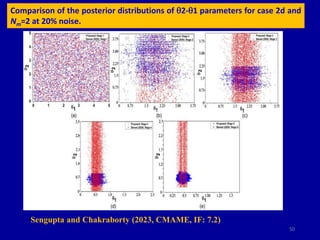
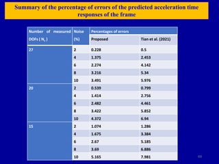
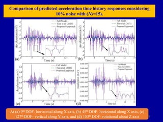
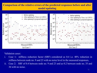
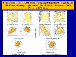
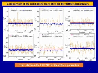
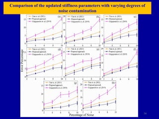
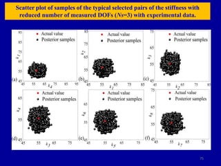
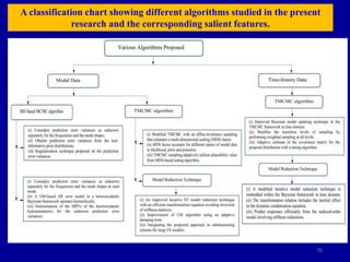
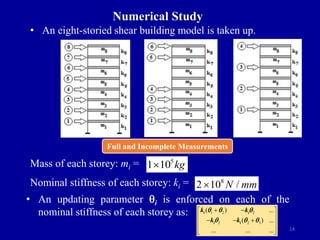
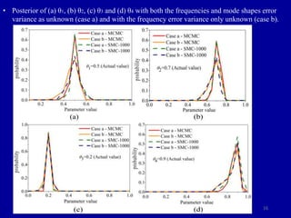
The document describes Bayesian model updating research using adaptive Bayesian filters and data-centric approaches. It outlines previous contributions, future research plans, and short-term objectives. The focus is on Bayesian updating with MCMC and TMCMC approaches to more accurately and efficiently update model parameters. Model reduction techniques are proposed in the frequency domain and time domain to address incomplete measured responses. Numerical studies on a shear building model demonstrate that the Bayesian updating algorithm can estimate parameters well when using 45 data sets and hyperparameters of 0.001, 0.001, with a maximum error of 2.5%.

1. Adaptive Bayesian filters and Data-centric
approaches in Model Updating
By
Dr. Partha Sengupta
Former Research Fellow
Department of Civil Engineering, Indian Institute of
Engineering Science and Technology, Shibpur
Presentation for the Position of Institute Post Doctoral Fellow

2. 2
Outlines of the Presentation
Research contributions so far
Future long-term research plans and goals
Short-term research objectives (next one year) and the
topic/content of possible first journal publication

3. 3
The focus of the present study is on:
Bayesian updating with MH-based MCMC and TMCMC approaches
for more accurate and efficient updating of model parameters.
To address the incompleteness of measured responses with the model
reduction techniques in the frequency domain and in the time domain.
Specifically
• Error Variance Models with MH-based MCMC
• TMCMC with model reduction using modal data
• TMCMC with model reduction in time domain

4. 4
Bayesian updating algorithm is proposed with homoscedastic and
heteroscedastic prediction error variance models.
 The prediction error variance models for non-informative prior estimation are
considered for both the frequencies and mode shapes.
 Three different choices of the hyperparameters are explored with each set
representing a prediction error model.
 The ill-conditioning problem is addressed by an improved regularization approach
based on the hyperparameters of the prediction error variances within the MH-
based MCMC algorithm.
 Then a Gaussian Mixture (GM) based Auto-regressive (AR) model in conditional
heteroscedastic (CH) (termed as GMARCH) framework is developed.
 The most probable values (MPVs) of the heteroscedastic parameters for the modal
observables are directly estimated using the suggested heteroscedastic error model
within the MH-based MCMC algorithm.
 The effectiveness of the proposed algorithm is illustrated numerically using an
eight-story shear building model and an experimental dataset examined at Los
Alamos National Laboratory (LANL).

5. 5
 A two-stage Bayesian model updating framework based on an affine-invariance
sampling in the TMCMC algorithm is explored.
 In the first stage, the proposed model reduction technique obtains the
transformation equation is expressed as a function of available modal responses
and mass matrices (usually invariant) only but eliminates the stiffness terms.
 The proposed model reduction technique is further integrated with a sub-
structuring scheme so that it can be easily applied to large FE models.
 In the second stage, an affine-invariance sampling approach is proposed to
estimate a multi-dimensional scaling (MDS) factor that accounts for the
frequencies and mode shapes.
 The effectiveness of the proposed algorithm is first demonstrated by considering
a simply-supported steel beam, a realistic ten-storied reinforced concrete (RC)
building.
A Bayesian updating algorithm is proposed along with an improvement in the
model reduction technique with modal data.

6. 6
 An improved Bayesian model updating technique in the TMCMC framework
in the time domain is investigated.
 An improved transformation equation is first obtained by expanding the
reduced structural matrices where the inertial effect is included in each term
of the dynamic condensation equation making it less dependent on the
selection of master DOFs.
 Further, the TMCMC algorithm is modified where the sample weights and the
scale of the proposal distribution for the random walk is adjusted accordingly.
 The efficiency of the algorithm is demonstrated considering simulated data of
a multi-storied frame and the available experimental dataset tested at LANL.
A Bayesian updating algorithm is proposed along with an improvement in the
model reduction technique in the time domain.

7. 7
Proposed Bayesian Model
Updating: Homoscedastic
Approach
Sengupta and Chakraborty (2022, SEM, IF: 3.534)

8. 8
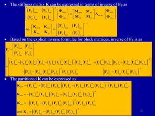
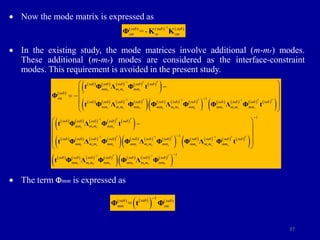
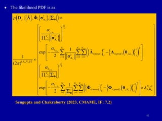
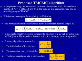
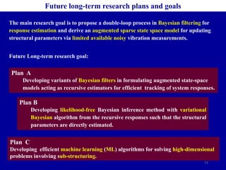
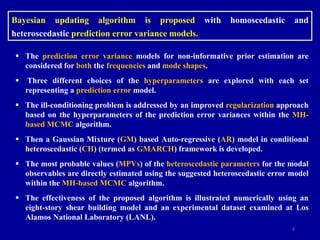
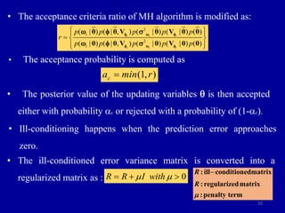
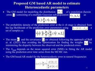
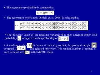
• The likelihood of outcome (D= w, f) for a parameter vector q:
2
2
ˆ
[ ( )]
1
( | ) exp
2
2 i
i
i i
i
p
w
w
w w
w

 

 
 
 
 
 
θ
θ
σ
σ
1
/2 1/2
1 1
( | ) exp ( ) ( )
(2 ) 2 i
i
T
i i i
i i
n
p 
 
   
   
 
   
 
θ V θ
V
f
f
f q f f f f

• The covariance matrix of mode shapes is as
where, is the variance of the mode shapes.
• The variance of mode shapes from dynamic test data is as:
2 2
, ,
1 1
1 1
ˆ ˆ
|| ||
i
J J
i j i j
j j
σ
Jm J
 
 
 
 
 
 
 
 
 
 
f f f
• The final representation of likelihood function is as:
2 2
1
( | ) ( | , ) ( | , ) ( | ) ( | )
i i i i i
m
i
i
p p p p p

 
D θ θ θ V θ V θ
w f w f
w  f 
2
i i
f f

 
V I
o o
n n
R 

I
2
i
f

where,

9. 9
• The prior distributions of the error variances for w and f, as:
• Sun and Büyüköztürk (2016) has adopted values as a1, b
2 2( 1)
2
( ) ( , ) exp
( )
i i
i
p IG
Ga
a
a
w w
w
b b
 a b 
a 
 
 
  
 
 
 
( 1)
( ) ( , ) exp
( )
i i
i
p IG
Ga
a
a
f f
f
b b
a b
a
 
 
  
 
 
 
V V
V
• A higher value of 1 for a and a very low value of b makes the
prediction error variance distribution concentrated.
• In the present study, the values of of a is decreased and b is
increased and both kept same.
• The hyperparameters are taken as 0.1, 0.01 and 0.001.
16
1 10


10. 10
• The acceptance criteria ratio of MH algorithm is modified as:
2
2
( | ) ( | , ) ( | ) ( | ) ( )
( | ) ( | , ) ( | ) ( | ) ( )
i i i
i i i
i
i
p p p p p
r
p p p p p
 
 
  
 
 
θ θ V θ V θ θ
θ θ V θ V θ θ
f w f
f w f
w f 
w f 
• The acceptance probability is computed as
• The posterior value of the updating variables q is then accepted
either with probability ac or rejected with a probability of (1-ac).
(1, )
c
a min r

• Ill-conditioning happens when the prediction error approaches
zero.
• The ill-conditioned error variance matrix is converted into a
regularized matrix as :

:ill conditionedmatrix
:regularizedmatrix
:penalty term
R
R

0
R I wi
R th
 
  

11. 11
• The regularization parameters are obtained as
 
 
1
,
i con
min mean r
 a

ω
 
 
2
,
i con
min mean r
f
 a

• The regularized prediction error variance matrices are obtained as:
2 2
ireg i i

 
ω ω ω
σ σ I
2 2
ireg i i
f f f



V V I
i. The value of the shape parameter used in obtaining the prior
distribution of the prediction error variances.
ii. Reciprocal condition number (rcon) of the error matrices
obtained by using the symbolic Math toolbox.
• The penalty term  is determined from the minimum value of the
following:

12. 12

13. 13
Sequential Monte Carlo (SMC) approach
• The SMC approach samples posterior PDF using a combination
of importance sampling and resampling mechanisms at different
levels (Au and Wang 2014) .
• The goodness of fit function is as:
• The importance weight updating is expressed as,
• The effective sample size (ESS) is as (Yang and Lam, 2018):
     
T
1
ˆ
( ) ( ) ( ) ( )
m
i i
i i i i
i
ω -ω f f f f

 
    
 
 

θ θ θ θ
       
1
1:g 1:g 1 g 1 g
( ) ( ) ( , )
g g g
w w w
  

θ θ θ θ
 
( ) ( ) 2 1
1
ESS( ) ( ( ) )
ss
N
h h
g g
h
w w 

 

14. 14
Numerical Study
• An eight-storied shear building model is taken up.
Full and Incomplete Measurements
Mass of each storey: mi =
• An updating parameter qi is enforced on each of the
nominal stiffness of each storey as: 1 2 2
2 2 3
( ) ...
( ) ...
... ... ...
 
 
 
  
 
 
 
i i
i i
k k
k k
q q q
q q q
5
1 10 kg

Nominal stiffness of each storey: ki = 8
2 10 /
N mm


15. 15
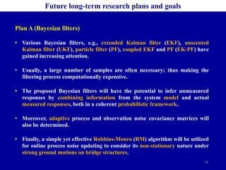
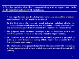
Actual
values
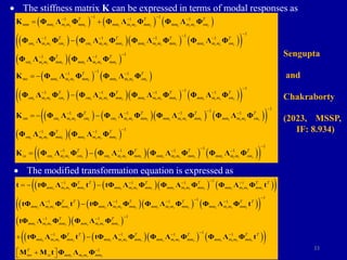
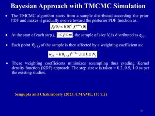
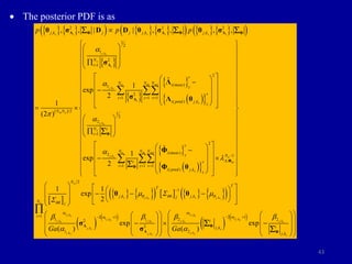
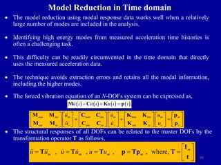
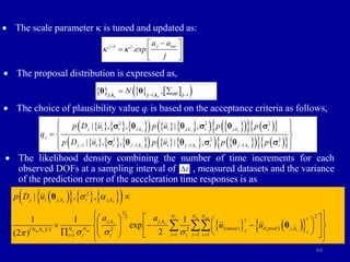
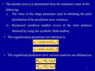
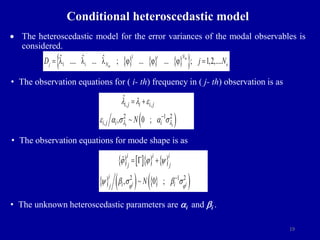
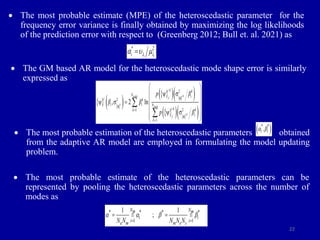
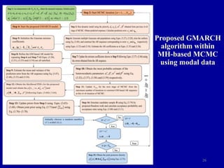
The posterior mean, standard deviation and percentage of errors (in square bracket) of
the parameters for different choice of hyper parameters and different data sets
(a,b) = (0.1,0.1) (a,b) = (0.01,0.01) (a,b) = (0.001,0.001)
15 sets 30sets 45sets 15sets 30sets 45sets 15sets 30sets 45sets
=0.5 0.55,0.11
[10.6]
0.54, 0.11
[7.1]
0.52,0.10
[4.6]
0.45,0.10
[9.1]
0.46, 0.09
[7.1]
0.48,0.08
[4.0]
0.48, 0.05
[3.8]
0.49, 0.05
[1.7]
0.49,0.04
[0.5]
=0.7 0.63,0.10
[9.8]
0.66,0.09
[5.1]
0.67,0.09
[3.1]
0.76,0.08
[8.7]
0.75,0.08
[8.2]
0.74,0.07
[6.5]
0.72,0.07
[3.5]
0.71,0.07
[1.8]
0.71,0.07
[1.5]
=0.2 0.24,0.05
[18.8]
0.22,0.04
[12.2]
0.21,0.04
[5.1]
0.22,0.04
[11.6]
0.22,0.04
[10.7]
0.21,0.04
[6.25]
0.22,0.04
[10.2]
0.21,0.04
[5.1]
0.20, 0.03
[2.5]
=0.9 0.79,0.14
[11.6]
0.79,0.14
[11.6]
0.82,0.13
[8.7]
0.95,0.09
[6.0]
0.93,0.07
[3.8]
0.93,0.05
[3.2]
0.85,0.08
[5.2]
0.87,0.08
[3.1]
0.88,0.07
[2.2]
=0.6 0.63,0.10
[5.8]
0.63,0.09
[4.6]
0.61,0.08
[2.0]
0.62,0.08
[3.6]
0.61,0.08
[2.2]
0.61,0.07
[1.7]
0.62,0.06
[4.0]
0.61,0.06
[2.0]
0.60,0.05
[0.2]
=1.0 0.88,0.12
[11.7]
0.91,0.11
[8.9]
0.93,0.10
[7.3]
0.90,0.11
[9.8]
0.91,0.10
[8.7]
0.93,0.09
[6.8]
0.95,0.08
[4.5]
0.97,0.08
[2.9]
0.98,0.07
[1.9]
=0.8 0.75,0.09
[6.1]
0.77,0.09
[3.2]
0.79,0.05
[1.0]
0.84,0.05
[5.1]
0.84,0.05
[4.4]
0.82,0.05
[2.7]
0.75,0.01
[5.8]
0.77,0.08
[3.6]
0.78,0.08
[2.2]
=0.4 0.34,0.14
[15.6]
0.35,0.13
[11.4]
0.38,0.12
[4.7]
0.42,0.07
[6.8]
0.42,0.06
[5.4]
0.41,0.06
[2.8]
0.41,0.06
[4.7]
0.41,0.06
[4.4]
0.41,0.05
[2.4]
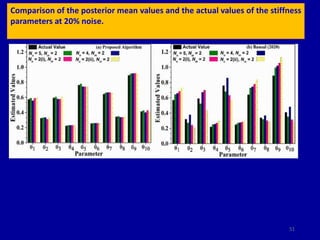
Comparison of actual and predicted parameters
• It can be noted that the posterior mean values are well estimated at 45 data sets with hyper
parameter values of (0.001, 0.001) with maximum error percentage of 2.5% for .
3
q

16. 16
• Posterior of (a) θ1, (b) θ2, (c) θ3 and (d) θ4 with both the frequencies and mode shapes error
variance as unknown (case a) and with the frequency error variance only unknown (case b).

17. 17
Proposed GM based AR conditionally
Heteroscedastic hierarchical error model
within MH-based MCMC algorithm
Sengupta et al. (ASCE-ASME J Risk Uncert. Part A, Revisions
submitted after positive round of reviews)

18. 18
An Autoregressive, heteroscedastic, hierarchical
model for Bayesian Updating
 Conventional Bayesian updating assumes a Gaussian distribution for modelling
the error in the observables (e.g., Modal parameters), which implies equal
variances at all modes, which is referred as homoscedasticity.
• The hierarchical Bayesian updating procedure presented by Behmanesh et al.
(2015) was adopted to efficiently embed the heteroscedasticity in the observation
equations.
• The present study attempt to improve on the selection of associated hyper
parameters with heteroscedastic framework by employing Gaussian Mixture
(GM) based Auto regressive (AR) model for the errors.
• The model is implemented using the Metropolis-Hastings (MH) based sampling
of the joint posterior for the MCMC simulation.

19. 19
Conditional heteroscedastic model
 The heteroscedastic model for the error variances of the modal observables is
considered.
• The observation equations for ( i- th) frequency in ( j- th) observation is as
• The observation equations for mode shape is as
• The unknown heteroscedastic parameters are ai and bi .
     
 
1
1
ˆ ˆ ˆ
.... ... ; ... ... ; 1,2,....
m
m
i N
j i N e
D j N
       
 
, ,
2 1 2
,
ˆ
, ~ 0 ;
i i
i j i i j
i j i i
N
 
  
 a  a 

 
      
     
 
2 1 2
ˆ
, ~ 0 ;
i i
i i i
j j
i
i i
j
N
 
  
 b  b 

  

20. 20
Proposed GM based AR model to estimate
Heteroscedastic parameters
 The GM model for modelling the distribution of a population (herein
error, ) consisting of a multiple Gaussian sub-population as
• The probability density of the prediction error at the k- th stage is obtained from
the log likelihoods of the prediction error parameters using a
set of samples as
• The mean and the covariance are obtained following the approach of Bull
et. al. (2021) thus avoiding the optimization for finding the weights by
minimizing the disparity between the observed and the predicted errors.
• The Ntrain depends on the mean squared error (MSE) in fitting the AR model
using the prediction error time series from the MCMC run.
• The GM based AR model for the heteroscedastic error in natural frequencies
   
, ,
1
| ,
k
N
i j m i j m m
m
p N

ε ε μ

 

 
   
, ,
1 1
ln ln | ,
train k
i j i j
N N
k k
m m m
k m
p N

ε ε μ
 
 
 
 
 
 
 
 
i,j
p ε
i,j
ε
 
i,j m m
N ,
ε μ Σ
{ :1,2,......, }
k train
N k N

m
μ m

 
m

 
  
  
,
,
2
2
2
1
1
, 2 ln
order k
i j i
train
i
k
i j i
k k
N
i
k
i i i N
k k
k
i
k
p α
ε α α
p α





 
 

 
 
 

 
 


ε
ε

21. 21
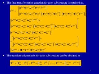
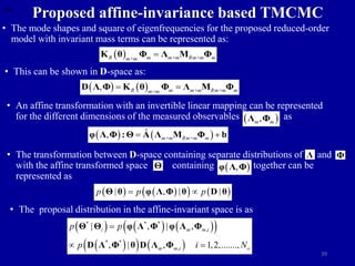
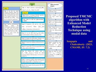
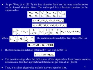
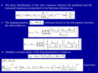
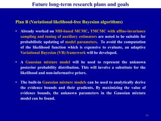
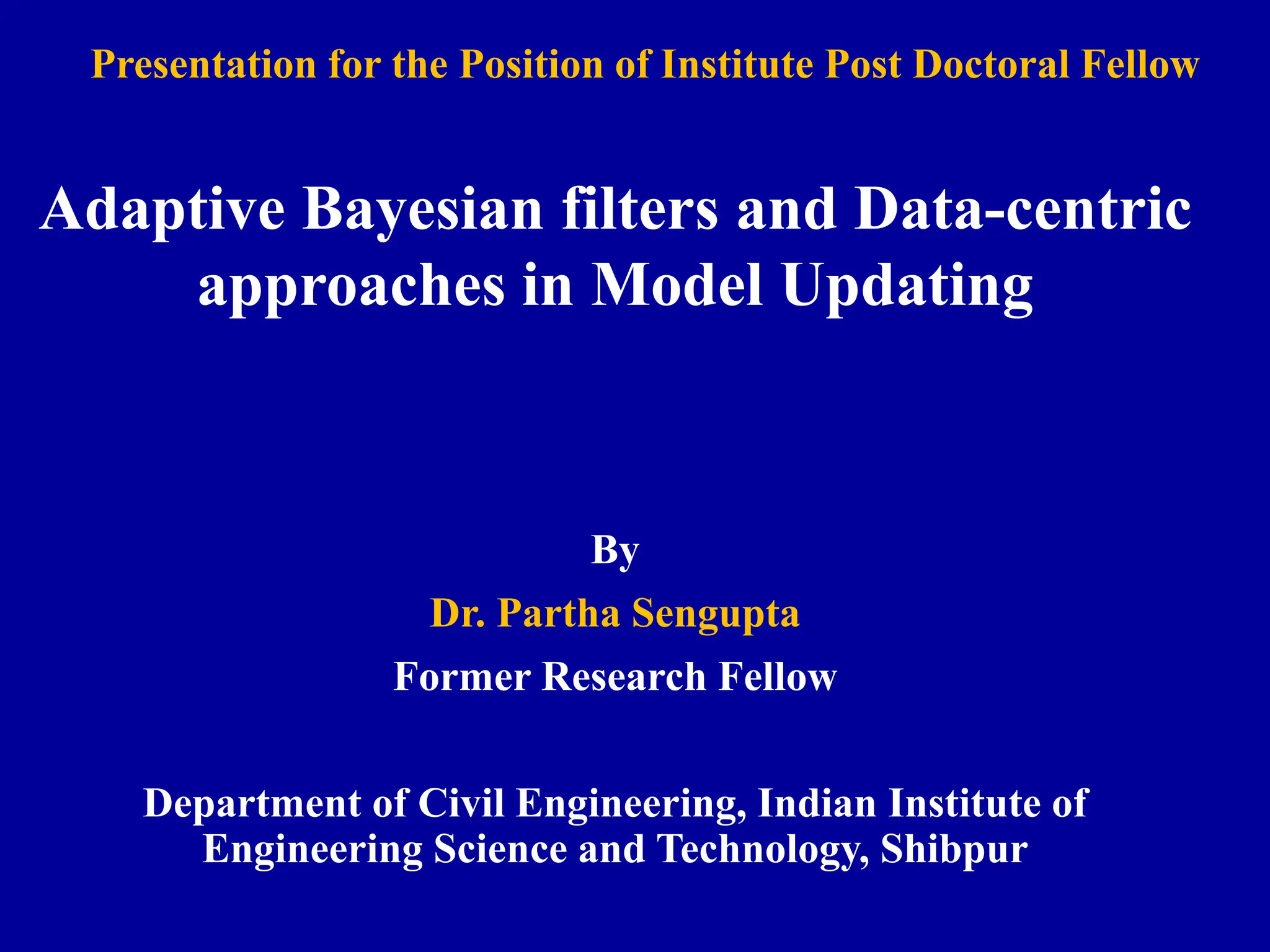
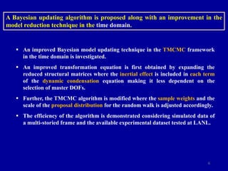
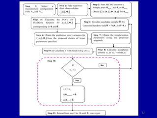
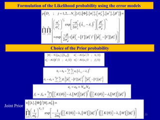
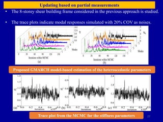
 The mean and the variance of the prediction error for the natural frequencies
become
 The outliers in the prediction errors are suitably trimmed using a methodology
for outlier detection from the probability of individual data points by Yuen and
Mu (2012)
 An expected Bayesian loss for the adaptive AR model considering the number
of measured DOFs (No) is as
 A confidence level cL is selected for use in a chi-square distribution
approximated from , denoted as
 The AR model is adaptively refined till
train train
i
N N
k k k
i 1 i 1 i
k 1 k 1
2 ( ( ) ( ))

 a  a  a
 
 
 
 
train train train
i
N N N
2
k k k k
i 2 i i 2 i
k 1 k 1 k 1
4 ( ( ) ( ( ))

 a  a a  a
  
  
 
1
1 [1/( 1)]
1 1
2 2 train
k N

 
 
   
 
 
 
m i
i
i
i
2
N i i
s s
i 1
ε ,
LR 2(N 1) (N 1)




a  



 

 
   
 
 
 
m
i
i
i
N
i 1
s
1
(N 1)










i
LR
2
( 1),
s
N 
 
2
( 1),
i i s
N
LR  
  


22. 22
 The most probable estimate (MPE) of the heteroscedastic parameter for the
frequency error variance is finally obtained by maximizing the log likelihoods
of the prediction error with respect to (Greenberg 2012; Bull et. al. 2021) as
 The GM based AR model for the heteroscedastic mode shape error is similarly
expressed as
 The most probable estimation of the heteroscedastic parameters obtained
from the adaptive AR model are employed in formulating the model updating
problem.
 The most probable estimate of the heteroscedastic parameters can be
represented by pooling the heteroscedastic parameters across the number of
modes as
* 2
i i
i  
a  

   
 
 
   
 
 
   
 
2
2
2
1
1
, 2 ln
i k
order
i
train
i k
i k k
N i
j
i k
i i N
i k k
k
i
j
k
p β
β β
p β
f
f

f

 
 
 
 
  
 
 
 
 


 
* *
i i
,
a b
* * * *
1 1
1 1
;
N N
m m
i i
i i
e m m e s
N N N N N
a a b b
 
 
 

23. 23
Formulation of the Likelihood probability using the error models
Choice of the Prior probability
Joint Prior
         
 
 
         
 
2 2 * *
1
2
* * *
2
,
2 2 2
1 1
2
; 1,2,... , , , , ,
ˆ
exp
2
ˆ ˆ
exp ( )
2
s
m e i
i i
i
j e
N
i i i
i j i
N N
i j i i
i i
T
i
j j
p D j N  f
  f
f
   a b
a a b
 
  
b
f f f f

 
 
  
 
 
 
   

 
 

   
   
 
 
 
    
 
 
 

    
 
 
 
 
 
 

     
   
   
2 *
1
2 * 2
1 1 1
~ , ~ 2 ; 2
~ 2 ; 2 2 ; 2
N IG b
IG d IG e f
q qq 
f q
q    a
 b 
 
    
      
 
2
1 0 ,
1 1
1 0
1 1
ˆ
ˆ ˆ
N N
m e
i i j i
i j
T
i i
N N i i
m e
i
j j
i j
b b
d d
a  
b f f f f
 
 
 
 
  
     
     
       
 
1 0
1 0
1
m d
T
N i i
m
i i
i
e e N N
f f K M K M
q  f q  f


 
   
   
   
   
   
     
 
     
       
 
2
2
2 2
1
, ,
1 1
exp
2
d
m
N
N T
i i
i i
i
K M K M
q
 q q
   q  
   
   
 q   f q   f
   
   
   
   
 
   


24. 24
Joint Posterior density
Improved MH algorithm for implementing the proposed model
       
         
     
     
1
2
* * *
2 2
2 2 2
,
2 2 2
1 1
*
1
2
2
2 2
ˆ
( , , , , , ) exp
2
ˆ ˆ
exp ( )
2
1 1
exp
2
S
m e
d
N
N N
i i i
i j i
i i i
i i
i i
T
i
i
j j
N
T
i
i i
S
K M K M
 f q
  f
f
f
q q
a a b
  q     
   
b
f f f f

q  f q 
 
 

 
   

    
     
     
 
  
 
    
 
 
   
 
 
 
   
   
   
     
  
 

 
 
   
       
 
*
*
1
1
2
1 1
2 2
1 1
2 2
1 1
2 2 2 2
1 1
exp exp
2 2
1 1
exp exp
2 2
i
T
e
b
d f
a
q qq q
 
b
f f q q
f
q  q 
 
   


 
 
 

 
   

 
       
 
     
       
 
 
       
       
   
  2
qq q

  I
• The proposal distribution is adopted to be from the acceptance/rejection criteria
in the MH draw as
     
 
,
N qq
 
θ θ priori

25. 25
• The acceptance probability is computed as
• The acceptance criteria ratio (Sedehi et. al. 2016) is calculated as
• The posterior value of the updating variables q is then accepted either with
probability or rejected with a probability of
• A random number is drawn at each step so that, the proposal sample i s
accepted if and rejected otherwise. This random number is updated at
each iteration step in the MCMC chain.
(1, )
c
a min r

               
   
 
               
   
 
2 2 2 2
2 2 2 2
( | , , , , ) ( , | ) ( ) , ,
( | , , , , ) ( , | ) ( ) , ,
j
j
p
r
p
 
 
  
 
 
D θ θ θ θ θ
D θ θ θ θ θ
 f  f
 f  f
 f     f     
 f     f     
c
a  
1 c
a

 
r
c
r a

 
itr
 
q

26. 26
Proposed GMARCH
algorithm within
MH-based MCMC
using modal data

27. 27
Updating based on partial measurements
• The 8-storey shear building frame considered in the previous approach is studied.
• The trace plots indicate modal responses simulated with 20% COV as noises.
Trace plot from the MCMC for the stiffness parameters
Proposed GMARCH model-based estimation of the heteroscedastic parameters

28. 28
AR model estimated heteroscedastic parameters for 20 percent noise
Modal assurance criterion vaues between the measured and updated mode
shapes for 20 percent noise
   
     
     
     
 
2
ˆ ˆ ˆ ˆ
,
T T T
MAC        


29. 29
Proposed Model Reduction Technique
using Modal Data
Sengupta and Chakraborty (2023, MSSP, IF: 8.934)

30. 30
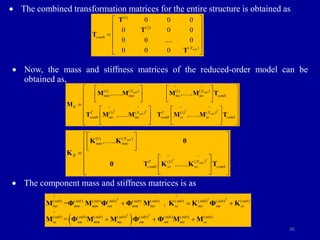
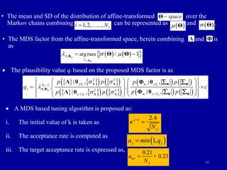
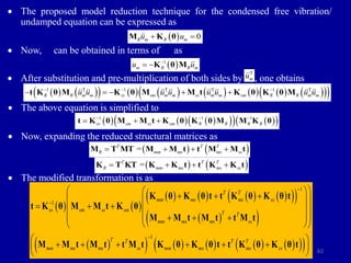
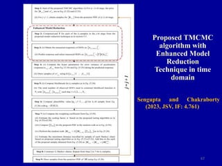
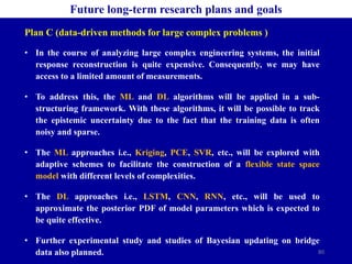
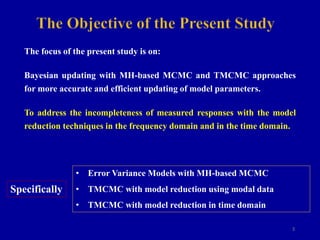
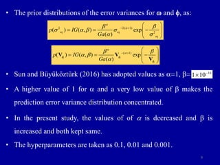
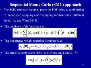
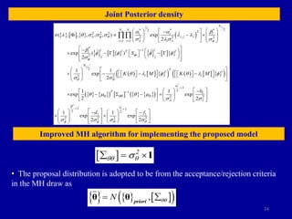
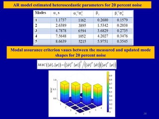
Model Reduction Formulation
 The generalized n-DOF linear system with M and K(θ) governed
by number of master (m) and slave (s) DOFs is as:
 The mode matrix for sm in terms of mm is as:
 The resulting equation for transformation parameter t is as:
 Transformation matrix T is as:
 The reduced M and K(θ) are as:
( ) ( )
( ) ( )
mm ms mm mm
mm
sm ss sm sm
   
   

   
   
   
   
mm ms
sm ss
K θ K θ Φ M M Φ
Λ
K θ K θ Φ M M Φ
sm mm

Φ tΦ
1 1 1
( ) ( ) ( )[ ]
T
ss ms ss ms ss mm mm mm
  
   
T
t K θ K θ K θ M M t Φ Λ Φ
T T
R R
and ( ) ( )
 
M T MT K θ T K θ T
 
T

T I t

31. 31
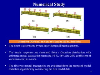
 The mode shape representing slave dofs s in terms of master dofs m for mr
number of modes m<< mr as
 The mode matrix is formulated as:
 The resulting formulation is as:
Proposed Transformation Formulation
 The flexibility matrix of a global structure, Fg can be obtained from its
vibration properties as,
1
F Φ Λ Φ

 T
g d d d
 Fg can be expressed for first mr modes as,
   
   
1 1
1
1 1
r r r r r r
r r r
r r r r r r
T T
g g
mm m mm mm m sm mm ms
T
g m m m T T
sm m mm sm m sm g g
sm ss
 

 
 
 
 
  
 
 
 
   
F F
Φ Λ Φ Φ Λ Φ
F Φ Λ Φ
Φ Λ Φ Φ Λ Φ F F
r r
sm mm

Φ tΦ
 
r r
mm sm

T
Φ Φ Φ
1 1 1
( ) ( ) ( )[ ] r r r
ss ms ss ms ss mm mm mm
  
   
T T
t K θ K θ K θ M M t Φ Λ Φ

32. 32
 The stiffness matrix K can be expressed in terms of inverse of Fg as
   
   
   
   
1
1
. .
r r
r r
r r
g g mm mm
mm ms mm ms
m m
sm ss
sm sm
g g
sm ss
g g
mm ms
mm ms
sm ss g g
sm ss


     
 
   
  
   
 
   
   
   
 
 
   

   
   
F F Φ Φ
M M
Λ
M M
Φ Φ
F F
F F
K K
i e
K K F F
 Based on the explicit inverse formulae for block matrices, inverse of Fg is as
   
   
             
                 
 
       
             
 
1
1
1 1
1 1 1 1 1 1
1 1
1 1 1
g g
mm ms
g
g g
sm ss
g g g g g g g g g g g g g g g
mm mm ms ss sm mm ms sm mm mm ms ss sm mm ms
g g g g g g g g g g
ss sm mm ms sm mm ss sm mm ms


 
     
 
  
 
 

 
 
 
   
 
  
 
  
 
 
F F
F
F F
F F F F F F F F F F F F F F F
F F F F F F F F F F
 The partitioned K can be expressed as
             
     
           
 
       
     
       
 
1
1 1 1 1
1
1 1
1
1 1
1
1
and
mm g g g g g g g g g
mm mm ms ss sm mm ms sm mm
ms g g g g g g
mm ms ss sm mm ms
sm g g g g g g
ss sm mm ms sm mm
ss g g g g
ss sm mm ms
,
K F F F F F F F F F
K F F F F F F
K F F F F F F
K F F F F

   

 

 


  
  
  
 

33. 33
 The stiffness matrix K can be expressed in terms of modal responses as
     
      
 
  
   
1 1
1 1 1
1
1
1 1 1 1
1
1 1
1
1 1
r r r r r r r r r r r r
r r r r r r r r r r r r r r r r
r r r r r r r r
r r r r r r r r
T T T
mm mm m m mm mm m m mm mm m m sm
T T T T
sm m m sm sm m m mm mm m m mm mm m m sm
T T
sm m m mm mm m m mm
T T
ms mm m m mm mm m m sm
 
  


   

 

 
 

 
K Φ Λ Φ Φ Λ Φ Φ Λ Φ
Φ Λ Φ Φ Λ Φ Φ Λ Φ Φ Λ Φ
Φ Λ Φ Φ Λ Φ
K Φ Λ Φ Φ Λ Φ
Φ
      
 
      
 
  
 
1
1
1 1 1 1
1
1
1 1 1 1
1
1 1
1
r r r r r r r r r r r r r r r r
r r r r r r r r r r r r r r r r
r r r r r r r r
r r r r
T T T T
sm m m sm sm m m mm mm m m mm mm m m sm
T T T T
sm sm m m sm sm m m mm mm m m mm mm m m sm
T T
sm m m mm mm m m mm
T
ss sm m m sm sm


   


   

 


  
 
Λ Φ Φ Λ Φ Φ Λ Φ Φ Λ Φ
K Φ Λ Φ Φ Λ Φ Φ Λ Φ Φ Λ Φ
Φ Λ Φ Φ Λ Φ
K Φ Λ Φ Φ
    
 
1
1
1 1 1
r r r r r r r r r r r r
T T T
m m mm mm m m mm mm m m sm


  
Λ Φ Φ Λ Φ Φ Λ Φ
 The modified transformation equation is expressed as
      
 
      
 
  
1
1 1 1 1
1
1
1 1 1 1
1
1 1
1
r r r r r r r r r r r r r r r r
r r r r r r r r r r r r r r r r
r r r r r r r r
r r r
T T T T T T
mm m m mm mm m m mm mm m m mm mm m m mm
T T T T T T
mm m m mm mm m m mm mm m m mm mm m m mm
T T
mm m m mm mm m m mm
mm m m

   


   

 

  


t tΦ Λ Φ t tΦ Λ Φ Φ Λ Φ Φ Λ Φ t
tΦ Λ Φ t tΦ Λ Φ Φ Λ Φ Φ Λ Φ t
tΦ Λ Φ Φ Λ Φ
tΦ Λ Φ
      
 
1
1 1 1
1
r r r r r r r r r r r r r
r r r r
T T T T T T
mm mm m m mm mm m m mm mm m m mm
T
ms ss mm m m mm

  


 

 
t tΦ Λ Φ Φ Λ Φ Φ Λ Φ t
M M t Φ Λ Φ
Sengupta
and
Chakraborty
(2023, MSSP,
IF: 8.934)

34. 34
Integration with Substructuring scheme
 The whole structure is divided into several substructures, and the
transformation matrices are constructed for each substructure.
 The reduced-order model obtained for each substructure are then assembled to
obtain a reduced-order model for the entire structure.
 Each substructure is generally divided into master, slave and interface DOFs.
 The master DOFs are usually selected based on the interface DOFs such that
the substructure matrices can be properly assembled.
 This involves consideration of a significant number of fixed-interface and
interface constrained modes and becomes inefficient for problems with a large
number of DOFs at the interface between substructures.
 The eigenvalue problem for substructure sub, where, can be
expressed in partitioned form as,
( ) ( )
( ) ( ) ( ) ( )
( )
( ) ( ) ( ) ( )
( ) ( )
r r
r r
r r
sub sub
sub sub sub sub
mm mm sub
mm ms mm ms
m m
sub sub sub sub
sub sub
sm ss sm ss
sm sm
   
   
   

   
   
   
   
   
Φ Φ
K K M M
Λ
K K M M
Φ Φ
1,2, ..., sub
sub N

Sengupta and Chakraborty (2023, MSSP, IF: 8.934)

35. 35
 The final transformation equation for each substructure is obtained as,
 The transformation matrix for each substructure can be obtained as
 
         
 
       
       
         
 
         
 
       
1
1 1 1
1
1
1
T T
r r r r
T T T T
r r r r r r r r r r r r
T T
r r r r
r r r r
sub sub sub sub sub
mm m m mm
sub
sub sub sub sub sub sub sub sub sub sub sub
mm m m mm mm m m mm mm m m mm
sub sub sub sub sub
mm m m mm
sub sub sub sub
mm m m mm

  



 

 
  
 
 

t Φ Λ Φ t
t
t Φ Λ Φ Φ Λ Φ Φ Λ Φ t
t Φ Λ Φ t
t Φ Λ Φ
       
         
 
       
       
 
         
 
       
   
1 1
1 1
1
1
1
1
1
T T T T
r r r r r r r r
T T
r r r r r r r r
T T
r r r r
T
r r r r r
sub sub sub sub sub sub sub
mm m m mm mm m m mm
sub sub sub sub sub sub sub
mm m m mm mm m m mm
sub sub sub sub sub
mm m m mm
sub sub sub sub sub
mm m m mm mm m
 
 





 
 
 
 
 


Φ Λ Φ Φ Λ Φ t
t Φ Λ Φ Φ Λ Φ
t Φ Λ Φ t
t Φ Λ Φ Φ Λ   
       
 
       
1 1
1
1
( ) ( )
T T
r r r r r r r
T
r r r r
sub sub sub sub sub
T
m mm mm m m mm
sub sub sub sub
sub sub
ms ss mm m m mm
 


 
 
 
 
 
 

 
Φ Φ Λ Φ t
M M t Φ Λ Φ
     
( ) ( ) ( )
(1) (1) (1) (2) (2) (2)
, ,.....,
T I t T I t T I t
  
sub sub sub
T
T T N N N
mm mm mm

36. 36
 The combined transformation matrices for the entire structure is obtained as
 Now, the mass and stiffness matrices of the reduced-order model can be
obtained as,
 The component mass and stiffness matrices is as
(1)
(2)
( )
0 0 0
0 0 0
0 0 .... 0
0 0 0 sub
comb
N
 
 
 

 
 
 
T
T
T
T
( ) ( )
(1) (1)
( ) ( )
(1) (1)
sub sub
T T
T T
sub sub
^
^
N N
mm mm ms ms comb
R ^ ^
^ ^
N N
T T
comb ms ms comb ss ss comb
,....., ,.....,
,....., ,.....,
 
   
 
   
   
 

 
   
 
   
 
   
 
M M M M T
M
T M M T M M T
T
( )
(1)
( )
(1)
sub
T
sub
N
mm mm
R ^
^
N
T
comb ss ss comb
,.....,
,.....,
 
 
 
 
 
 

 
 
 
 
 
 
 
K K 0
K
0 T K K T
 
T
T
( ) ( ) ( ) ( ) ( ) ( ) ( ) ( ) ( ) ( )
( ) ( ) ( ) ( ) ( ) ( ) ( ) ( )
T T
T
^ ^
sub sub sub sub sub sub sub sub sub sub
ms mm mm sm mm ms ss ms sm ss
^
sub sub sub sub sub sub sub sub
ss sm mm ms sm sm ms ss
= ,
=
  
  
M Φ M Φ Φ M K K Φ K
M Φ M M Φ Φ M M

37. 37
 Now the mode matrix is expressed as
 In the existing study, the mode matrices involve additional (m-mr) modes.
These additional (m-mr) modes are considered as the interface-constraint
modes. This requirement is avoided in the present study.
 The term mm is expressed as
1
( ) ( ) ( )
-
sub sub sub
sm ss sm
=

Φ K K
 
         
 
       
       
         
 
         
 
     
1
1 1 1
1
1
1
T T
r r r r
T T T T
r r r r r r r r r r r r
T T
r r r r
r r r r
sub sub sub sub sub
mm m m mm
sub
sm
sub sub sub sub sub sub sub sub sub sub sub
mm m m mm mm m m mm mm m m mm
sub sub sub sub sub
mm m m mm
sub sub sub s
mm m m mm

  



 

 
  
 
 

t Φ Λ Φ t
Φ
t Φ Λ Φ Φ Λ Φ Φ Λ Φ t
t Φ Λ Φ t
t Φ Λ Φ 
       
         
 
       
       
 
1 1
1 1
1
1
1
T T T T
r r r r r r r r
T T
r r r r r r r r
ub sub sub sub sub sub sub sub
mm m m mm mm m m mm
sub sub sub sub sub sub sub
mm m m mm mm m m mm
 
 



 
 
 
 
 
Φ Λ Φ Φ Λ Φ t
t Φ Λ Φ Φ Λ Φ
 
 
1
( ) ( )
sub
sub sub
mm sm
=

Φ t Φ

38. 38
Bayesian Approach with TMCMC Simulation
 The TMCMC algorithm starts from a sample distributed according the prior
PDF and makes it gradually evolve toward the posterior PDF function as:
 At the start of each step j, , the sample of size Ns is distributed as qj-1 .
 Each point qj−1,k of the sample is then affected by a weighting coefficient as:
 These weighting coefficients minimizes resampling thus evading Kernel
density function (KDF) approach. The step size k is taken = 0.2, 0.5, 1.0 as per
the existing studies.
( ) ( )
( ) 
θ θ θ
j
q prior
j
f l f
1  
j m
1
, 1,
( ) ,1



  
θ j j
q q
j k j k s
w l k N
Sengupta and Chakraborty (2023, CMAME, IF: 7.2)

39. 39
Proposed affine-invariance based TMCMC
• The mode shapes and square of eigenfrequencies for the proposed reduced-order
model with invariant mass terms can be represented as:
 
R m m×m Rm×m m
m×m

K θ Φ Λ M Φ
• This can be shown in D-space as:
   
, R m m×m Rm×m m
m×m
 
D Λ Φ K θ Φ Λ M Φ
• An affine transformation with an invertible linear mapping can be represented
for the different dimensions of the measured observables as
) as
 
,
m m
Λ Φ
   
ˆ
, m×m Rm×m m
 
φ Λ Φ : Θ A Λ M Φ b
• The transformation between D-space containing separate distributions of and
with the affine transformed space containing together can be
represented as
Λ Φ
Θ  
,
φ Λ Φ
   
   
| , | |
p p p
 
Θ θ φ Λ Φ θ D θ
• The proposal distribution in the affine-invariant space is as
     
 
 
   
* * *
,
* *
,
| , | ,
, | , 1,2,.......,
i m m i
m m i o
p p
p i N

 
Θ Θ φ Λ Φ φ Λ Φ
D Λ Φ θ D Λ Φ

40. 40
• The mean and SD of the distribution of affine-transformed over the
Markov chains combining can be represented as and .
) as
space

Θ
1,2,......., o
i N
  
 Θ  
 Θ
• The MDS factor from the affine-transformed space, herein combining and is
as
Λ Φ
   
 
,
, argmax / 1
m
m



  
 
Φ
Φ Θ Θ
 The plausibility value qj based on the proposed MDS factor is as
   
   
 
   
   
 
   
   
2 2
1
, 2 2
| , | ,
. .
| ,
| ,
s s
o
m
s
s
j,k m j,k
N
j
m j-1,k
j-1,k
p p p p
q c
p p
p p
 

 

 
   
 
   
 
 
 
 
 
 
 
 
Λ Λ Φ Φ
Λ Φ
Φ Φ
Λ Λ
Λ θ Φ θ
Φ θ
Λ θ
 
 
 A MDS based tuning algorithm is proposed as:
i. The initial value of k is taken as
ii. The acceptance rate is computed as
iii. The target acceptance rate is expressed as,
1 2.4
j
p
N
k 

 
1,
j j
a min q

0.21
0.23
tar
p
a +
N


41. 41
 The likelihood PDF is as
   
 
 
 
 
   
 
 
   
 
,
,
,
,
2
1
2
1
2
1
2
1
( ) ( ) ,
2
1 1 1
/2
1
2
2
1
2
( ) ( ) ,
1
ˆ ˆ
| , , ,
1 ˆ
exp
2
1
(2 )
1 ˆ
exp
2
i
j ks
o
i
o m set
j ks
s
i
m o
j ks
o
o
j ks
s
j
N
i
N N N v
v
i meas i pred j k
z z
i z v
N N
N i
i
N
v
i meas i pred j k
i z z
i
p
a
a

a
a

  



 
 
 

 
 
 
 
 
 

 
 
 

 
 
 

Λ Φ
Λ
Λ
Φ
Φ
D Λ Φ σ
σ
Λ Λ θ
σ
Φ Φ θ



 
2
1
,
1 1
m set
o
m
N N v
N
z v

 
 
 
 
 
 
 
 
 
 
 
 
 
 
 
 
 
 

 
 
 
 
 
 Φ
Sengupta and Chakraborty (2023, CMAME, IF: 7.2)

42. 42
 The prior PDF is as
     
 
 
   
       
 
 
 
 
 
, ,
1 ,
1 ,
, ,
,
, ,
2 ,
2 ,
,
,
2
,
2
1
, ,
2 1
1 1
2
2
1
2 1
2
,
2
| , ,
1 1
exp
2
exp
( )
exp
( )
s i
o
s j k s j k
s s
j ks
j ks
j k j k
s s
j ks
j ks j ks
j ks
j ks
j ks
s
j ks
j k
N
T
T
j k j k
j
j
i
j k
p
Ga
Ga
qq
q qq q
qq
a
a
a
a

  

b b
a
b
a

 
 

   
 
    
 
 
   
 
 
 
 
 
 
 
 
 
 
 
Λ Φ
Λ
Λ
Φ
θ σ
θ θ
σ
σ

 ,
1
2
,
o
j ks
s
N
i
i
j k
b

 
 
 
 

 
 
 
 

Φ


43. 43
 The posterior PDF is as
   
     
     
 
 
 
 
 
 
 
,
,
,
2 2 2
, , ,
1
2
1
2
1
2
( )
1
2
1 1 1
( ) ,
/2
1
2
2
1
, , | | , , , ,
ˆ
1
exp
2
1
(2 )
exp
s i s i s i
j ks
s
i
o m set
j ks
i
s
m o
j ks
s
j k j j j k j k
N
i
v
N N N i meas
z
v
i z v
i pred j k
z
N N
N i
i
p p p
a
a

a

  


 
 
 

 
 
 

 
 

 
 
 
 
 
 
 
 
 
 

 
 
Λ Φ Λ Φ Λ Φ
Λ
Λ
Φ
θ σ D D θ σ θ σ
σ
Λ
σ Λ θ
  

 
 
 
 
   
       
 
,
, ,
2
( )
2 1
,
1 1 1
( ) ,
2
1
, ,
1
ˆ
1
2
1 1
exp
2
o m set
j ks o
m
s
o
s j k s j k
s s
v
N N N i meas
z N
i v
i z v
i pred j k
z
N
T
T
j k j k
j
j

q qq q
qq
a

  

b

  

 
 
 
 
 
 
 
 
 
 
 
 
 
 
 
 
 
 

 
 
 
 
 
 
 
 
 
 
 
 
 
 
   
 
    
 
 
   
 
 
  Φ
Φ
Φ
Φ θ
θ θ

 
 
 
 
1 2
, ,
2
1 ,
,
, , , ,
,
, ,
,
1 2 1
2 1
1 2 2
2
2 ,
1 2
,
exp exp
( ) ( )
o
j k j k
s s
j k
j k s
s
j k j k j k j k
s s s s
j ks s
j k j k
s j k s
s s
N
i
i
i
j k
j k
Ga Ga
a a
a
a b b b
a a
  
   
   
 
 
   
 
  
 
   
 
   
   

Λ Φ
Λ Φ
σ
σ



44. 44
Proposed TMCMC
algorithm with
Enhanced Model
Reduction
Technique using
modal data
Sengupta and
Chakraborty (2023,
CMAME, IF: 7.2)

45. 45
Numerical Study
Measured DOFs: (a) at 5, (b) at 4, (c) and (d) at 2 locations
• The beam is discretized by ten Euler-Bernoulli beam elements.
• The modal responses are simulated from a Gaussian distribution with
estimated modal data as the mean and 10 %, 15% and 20% coefficient of
variation (cov) as noises.
• The first two natural frequencies are evaluated from the proposed model
reduction algorithm by considering the first modal data

46. 46
Comparison of the identification of the first two natural frequencies of the
beam for different number of measured dofs

47. 47
Modal assurance criterion values for 20 percent noise
• The reduced Rayleigh damping matrix can be obtained as,
   
i j
T
R 0 R 1 R 0 j i i j 1 j j i i
2 2 2 2
j i j i
2 2
a a , where a and a
C T CT M K
      
 
w w
w  w  w  w 
w w w w
• The amplitude of the complex FRFs and phase plots are obtained for the
actual and reduced system are as
1 1
 
 
  
 
 
0 I
A
M K M C 1 1
R
R R R R
 
 
  
 
 
0 I
A
M K M C

48. 48
Comparison of amplitude and phase for 2% and 10% damping at 10% noise
0 50 100 150 200 250
(a)
amplitude
(dB)
Frequency, w (rad/s)
Exact
Proposed
Bansal (2020)
40
30
0
20
10
0 50 100 150 200 250
(b)
amplitude
(dB)
Frequency, w (rad/s)
Exact
Proposed
Bansal (2020)
0
10
20
30
40
Amplitude at 2% damping Amplitude at 10% damping
0 50 100 150 200 250
(c)
phase
(deg)
Frequency, w (rad/s)
Exact
Proposed
Bansal (2020)
135
90
45
0
-45
-90
-135
0 50 100 150 200 250
(d)
phase
(deg)
Frequency, w (rad/s)
Exact
Proposed
Bansal (2020)
135
90
45
0
-45
-90
-135
Phase at 2% damping Phase at 10% damping

49. 49
Summary of computational time, maximum error percentage and MAC value
for the second modal frequency and mode shape of the beam under 20%
noise with Nm=1 and No=2 for case 2d.
Model reduction Computation
time (s)
Modal
Frequency
Mode shape
Error percentage Error
percentage
MAC
Proposed 2.8 0.18 0.2 0.9859
Bansal (2020) 5.3 1.96 3.07 0.9700
Tian et. al. (2019) 2.82 1.42 3.49 0.9862
Sun and Büyüköztürk
(2016) 4.13 2.11 4.46 0.9474
Jensen et. al. (2014) 3.41 1.75 3.91 0.9724
Xia and Lin (2004) 5.72 4.02 5.78 0.9305
Friswell et. al. (1995) 7.82 5.21 6.34 0.9228
Sengupta and Chakraborty (2023, MSSP, IF: 8.934)

50. 50
Comparison of the posterior distributions of q2-q1 parameters for case 2d and
Nm=2 at 20% noise.
Sengupta and Chakraborty (2023, CMAME, IF: 7.2)

51. 51
Comparison of the posterior mean values and the actual values of the stiffness
parameters at 20% noise.

52. 52
Example 2: A ten-storey building
Isometric view of the building model
• The building is modelled in ABAQUS 2020.
• The geometrical and material properties of the structure are adopted from
Jensen et. al. (2014).
• The floors of the building are modelled with shell elements with a thickness
of 0.3m and beam elements with rectangular cross section having dimensions
as taken by Jensen et. al. (2014).
• The number of dofs is about 40,000.

53. 53
Substructures from the finite element model
(Jensen et. al. 2014)

54. 54
Comparison of the maximum error percentage for the first and eleventh
modal frequency for different substructure cases
(a) Proposed (b) Bansal (2020)
0.0
0.2
0.4
0.6
0.8
First Modal Frequency (actual value=4.384 rad/s) (a)
Error
percentage
(%)
Number of measured dofs
Substructure Case1-10% noise Substructure Case2-10% noise
Substructure Case1-15% noise Substructure Case2-15% noise
Substructure Case1-20% noise Substructure Case2-20% noise
Substructure Case3-10% noise
Substructure Case3-15% noise
Substructure Case3-20% noise
30 40 50
0
5
10
First Modal Frequency (actual value=4.384 rad/s) (b)
Error
percentage
(%)
Number of measured dofs
Substructure Case1-10% noise Substructure Case2-10% noise
Substructure Case1-15% noise Substructure Case2-15% noise
Substructure Case1-20% noise Substructure Case2-20% noise
Substructure Case3-10% noise
Substructure Case3-15% noise
Substructure Case3-20% noise
30 40 50
0.0
0.3
0.6
0.9
Eleventh Modal Frequency (actual value=40.376 rad/s) (a)
Error
percentage
(%)
Number of measured dofs
Substructure Case1-10% noise Substructure Case2-10% noise
Substructure Case1-15% noise Substructure Case2-15% noise
Substructure Case1-20% noise Substructure Case2-20% noise
Substructure Case3-10% noise
Substructure Case3-15% noise
Substructure Case3-20% noise
30 40 50
0
5
10
15
20
Eleventh Modal Frequency (actual value=40.376 rad/s) (b)
Error
percentage
(%)
Number of measured dofs
Substructure Case1-10% noise Substructure Case2-10% noise
Substructure Case1-15% noise Substructure Case2-15% noise
Substructure Case1-20% noise Substructure Case2-20% noise
Substructure Case3-10% noise
Substructure Case3-15% noise
Substructure Case3-20% noise
30 40 50

55. 55
Comparison of the convergence of the eleventh modal frequency
(a) Proposed (b) Bansal (2020)
Modal assurance criterion values for 20 percent noise

56. 56
Amplitude at 2% damping Amplitude at 10% damping
Phase at 2% damping Phase at 10% damping
0
20
40
60
80
(a)
40
0 45
35
5 30
15 20
10 25
amplitude
(dB)
Frequency, w (rad/s)
Actual
Proposed
Bansal (2020)
0
20
40
(b)
0 35
5 30
15 20
10 25
amplitude
(dB)
Frequency, w (rad/s)
Actual
Proposed
Bansal (2020)
(c)
0 40
35
5 30
15 20
10 25
phase
(deg)
Frequency, w (rad/s)
Actual
Proposed
Bansal (2020)
0
90
180
-90
-180
(d)
0 40
35
5 30
15 20
10 25
phase
(deg)
Frequency, w (rad/s)
Actual
Proposed
Bansal (2020)
0
90
180
-90
-180
Comparison of amplitude and phase for 2% and 10% damping at 10% noise

57. 57
Summary of computational time, maximum error percentage and MAC value
of the 12th modal frequency and mode shape for substructure case 3 under
20% noise with Nm=4 and No=30.
Model reduction Computation
time (s)
Modal
Frequency
Mode shape
Error
percentage
Error
percentage
MAC
Proposed 1875 4.13 4.78 0.98
Bansal (2020) 9850 10.53 11.82 0.9604
Tian et. al. (2019) 8640 8.35 9.39 0.9765
Boo and Lee (2017) 9331.2 6.1 6.9 0.9381
Jensen et. al. (2016) 9611.1 6.6 7.4 0.9213
Sun and Büyüköztürk
(2016) 10353.6 14.3 17.1 0.9039
Xia and Lin (2004) 11676 16.6 20 0.8944
Friswell et. al. (1995) 14277.2 18 21.6 0.8871

58. 58
The identified posterior and marginal distributions of the unknown
parameters for No=30 and Nm=4 at 20% noise.

59. 59
Proposed Model Reduction Technique in
Time Domain
Sengupta and Chakraborty (2023, JSV, IF: 4.761)

60. 60
Model Reduction in Time domain
 The model reduction using modal response data works well when a relatively
large number of modes are included in the analysis.
 Identifying high energy modes from measured acceleration time histories is
often a challenging task.
 This difficulty can be readily circumvented in the time domain that directly
uses the measured acceleration data.
 The technique avoids extraction errors and retains all the modal information,
including the higher modes.
 The forced vibration equation of an N-DOFs system can be expressed as,
mm ms m mm ms m mm ms m m
sm ss s sm ss s sm ss s s
u u u
u u u
             
  
             
             
M M C C K K p
M M C C K K p
 The structural responses of all DOFs can be related to the master DOFs by the
transformation operator T as follows,
, , where, m
m m m m
u u , u u u u ,
 
      
 
I
T T T p Tp T
t
       
u u u
   
  
M C K p

61. 61
 As per Weng et al. (2017), the free vibration form has the same transformation
as the forced vibration form. The undamped free vibration equation can be
expressed as
0 0
T
ms ss
 
  
 
~
M
M M
Where, The reduced-order model by Tian et al. (2021) is
 The transformation relation obtained by Tian et al. (2021) is
 The iterations stop when the differences of the eigenvalues from two consecutive
iterations are less than a predefined tolerance as per Tian et al. (2021).
 Thus, it involves eigenvalue analysis at every iteration step.
0
mm ms m mm ms m
sm ss s sm ss s
u u
u u
     
 
     
     
M M K K
M M K K
 
1
s ss sm m ss s sm m
u u u u

   
K M M K
 
1
m ss sm m ss m sm m
u u u u

   
t K M M t K
1 1
0 0 0
m m
m m m G m m
T
s ss sm ss ms ss
u
u u u u u u
u  
      
     
      

      
~
I
T T T SMT
K K K M M
1
0 0 0
T
ss ms ss
,

   
 
   
   
~
S M
K M M
,
T T
d G G G G
 
M T MT K T KT
1
G d G

 
~
T T SMTM K

62. 62
 The proposed model reduction technique for the condensed free vibration/
undamped equation can be expressed as
 Now, can be obtained in terms of as
 After substitution and pre-multiplication of both sides by , one obtains
 The above equation is simplified to
 Now, expanding the reduced structural matrices as
 The modified transformation is as
   
       
 
 
 
 
 
         
 
 
1
1
1
T T
mm ms ms ss
ss sm ss sm
T T
mm ms ms ss
T T T T
mm ms ms ss mm ms ms ss



 
 
  
 
 
  
 
 
 
  
 
 
 
 
     
 
 
K θ K θ t t K θ K θ t
t K θ M M t K θ
M M t M t t M t
M M t M t t M t K θ K θ t t K θ K θ t
  0
R m R m
u u
 
M K θ
 
1
m R R m
u u

 K θ M
   
             
 
 
1 T 1 T T 1 T
R R m m ss sm m m ss m m sm R R m m
u u u u u u u u
  
    
t K θ M K θ M M t K θ K θ M
     
 
   
 
1 1 1
ss sm ss sm R R R R
  
  
t K θ M M t K θ K θ M M K θ
   
T T T
R mm ms ms ss
=
   
M T MT M M t t M M t
   
T T T
R mm ms ms ss
=
   
K T KT K K t t K K t
T
m
u

63. 63
Proposed TMCMC algorithm
 In the present study, for an improved estimate of transition PDFs, the maximum
likelihood PDF is obtained first from the samples at a particular stage and its
preceding stage of TMCMC.
 This is used to compute the weighting coefficient as:
 The proposal distribution covariance matrix is estimated from the sample as,
 k is a scaling factor chosen to suppress the rejection rate as well as tackle large
MCMC jumps. The step size k is taken = 0.2, 0.5, 1.0 as per the existing studies.
 A tuning algorithm is proposed as:
i. The initial value of k is taken as
ii. The acceptance rate is computed as
iii. The target acceptance rate is expressed as,
1 2.4
j
p
N
k 

 
1,
j j
a min q

0.21
0.23
tar
p
a +
N

( ) ,1
j j-1
q q
j,k max j-1,k j
l k N

  
θ s s
w
 
j j
N 1 N 1
T
j,k j-1,k j j-1,k j j j,k j-1,k
j
k =1 k =1
( )( ) with
qq k
 
    
 
θ m θ m m θ
s s s s s
s s
w w

64. 64
 The scale parameter k is tuned and updated as:
 The proposal distribution is expressed as,
 The choice of plausibility value qj is based on the acceptance criteria as follows,
 The likelihood density combining the number of time increments for each
observed DOFs at a sampling interval of , measured datasets and the variance
of the prediction error of the acceleration time responses is as
 
     
 
     
 
2
, ,
1
2
2
, ,
( ) ( ) ,
2 2
/2
1 1 1
1
| , ,
1 1 1
exp
2
(2 )
s s
s m set
s s
s
s m
m s
j i j k i j k
N N N v
v
j k j k
i meas i pred j k
N N
N N z z
i z v
i i
i i
p D u
a a
u u
 a
 

   


 
   
 
 
  
 
 
   
  
   
 
 
 
θ
θ
1
. j tar
j j
a a
exp
j
k k


 
  
 
     
 
1
, 1,
,
N qq 

 
θ θ
s s j
j k j k
     
     
   
 
   
 
     
     
   
 
   
 
2 2 2
2 2 2
1 1 1 1
| , , | ,
| , , | ,
s s s
s s s
j i i j,k i j,k i j,k i
j
j i i j ,k i j ,k i j ,k i
p D u p u p p
q
p D u p u p p
   
 
 
  
 
 
 q q  q 
 q q  q 
t


65. 65
 The prior distributions of the error variances between the predicted and the
measured responses incorporated in the Bayesian inference as,
 The hyperparameters estimated based on the discrepancy between
the observables as,
 Initially, a certain choice of the hyperparameters is made as:
Joint Prior
,
,
2( 1)
, ,
2 2
, , , , 2
, ,
( ) ( , ) ( ) exp
( )
j ks
j k
s s
s
s s s s
s s
j k j k
j k j k j k j k
j k j k
p IG
Ga
a
a
b b
 a b 
a 
   
  
 
 
 
   
 
 
2
( ) ( ) ,
1 1 1
( )
s m set
s
s s
v
v
N N N
i meas i pred j k
z z
j+1,k j,k v
i i v
i meas z
u u
a a
u
  
 

 
 
 
 
 

θ
 
 
 
 
 
 
2
( ) ( )
1 1 1
( ) , ( ) ,
1
s m set
s s
s s
T
v v
N N N
i meas i meas
z z
j+1,k j,k v v
i z v
i pred j k i pred j k
z z
u u
u u
b b
  
 
   
 
   
 
  
   
 
   
 
   
 

θ θ
,
,
and s
s
j k
j k
a b
;
j,k 0,0 m set j,k 0,0 m
s s
a a N N N
b b
   
   
 
 
   
       
     
,
, ,
,
2 1
2
1 ,
, , 1
1
1 1 1
exp exp
2
s
j ks
s
s
s
s j k s j k
s s
j k
N
T
N T
j k
j k j k
j
i
j j j
p qq
a
q qq q
qq qq qq
b
 




 
     
 
 
     
      
 
 
     
 
  
 
     

θ
θ θ

66. 66
Joint Posterior density
   
       
 
 
   
       
 
, ,
1
2
2
, ,
2
( ) ( ) ,
2 2
/2
1 1 1
1
2
1
, ,
1 1 1
, , exp
2
(2 )
1 1
exp
2
s m set
s s
s s
s m
m s
s
s j k s j k
s s
N N N v
v
j k j k
i j,k i i meas i pred j k
N N
z N N z z
i z v
i i
i
i
N
T
j k j k
j
j
a a
p u u u
q qq q
qq

 


 
  


 
 
 
 
 
   
 
 
 
 
 
  
 
 
 
 
 

     
  

 
 
θ θ
θ θ
   
,
1
2
,
1
1
1
exp
j ks
s
s
T
N
j k
i j j
a
qq qq
b



   
 
    
  
 
     
  
 
     

Sengupta and Chakraborty (2023, JSV, IF: 4.761)

67. 67
Proposed TMCMC
algorithm with
Enhanced Model
Reduction
Technique in time
domain
Sengupta and Chakraborty
(2023, JSV, IF: 4.761)

68. 68
Example 1: A nine-storey steel frame
Schematic diagram of the nine-storey steel frame
• The building is modelled in SAP2000.
• The geometrical and material properties are adopted from Tian et. al. (2021).
El centro ground motion

69. 69
Summary of the percentage of errors of the predicted acceleration time
responses of the frame
Number of measured
DOFs ( Ns )
Noise
(%)
Percentages of errors
Proposed Tian et al. (2021)
27 2 0.228 0.5
4 1.375 2.453
6 2.274 4.142
8 3.216 5.34
10 3.491 5.976
20 2 0.539 0.799
4 1.414 2.756
6 2.482 4.461
8 3.422 5.852
10 4.372 6.94
15 2 1.074 1.286
4 1.675 3.384
6 2.67 5.185
8 3.69 6.886
10 5.165 7.981

70. 70
Comparison of predicted acceleration time history responses considering
10% noise with (Ns=15).
At (a) 9th DOF- horizontal along X axis, (b) 45th DOF- horizontal along X axis, (c)
127th DOF- vertical along Y axis, and (d) 153th DOF- rotational about Z axis

71. 71
Comparison of the relative errors of the predicted responses before and after
model updating
Validation cases:
i. Case 1: stiffness reduction factor (SRF) considered as 0.4 i.e. 40% reduction in
stiffness between node no. 9 and 23 with no noise level in the measured responses,
ii. Case 2: SRF of 0.4 between node no. 9 and 23 and as 0.2 between node no. 35 and
36 with no noise.

72. 72
Comparisons of the TMCMC samples at different stages for the selected pairs
of q2-q1 the stiffness parameters with reduced number of measured DOFs
(Ns=15) at 10% noise.

73. 73
Comparisons of the normalized trace plots for the stiffness parameters
Trace plot from the TMCMC for the stiffness parameters

74. 74
Comparison of the updated stiffness parameters with varying degrees of
noise contamination

75. 75
Scatter plot of samples of the typical selected pairs of the stiffness with
reduced number of measured DOFs (Ns=3) with experimental data.

76. 76
A classification chart showing different algorithms studied in the present
research and the corresponding salient features.

77. 77
The main research goal is to propose a double-loop process in Bayesian filtering for
response estimation and derive an augmented sparse state space model for updating
structural parameters via limited available noisy vibration measurements.
Plan A
Developing variants of Bayesian filters in formulating augmented state-space
models acting as recursive estimators for efficient tracking of system responses.
Plan B
Developing likelihood-free Bayesian inference method with variational
Bayesian algorithm from the recursive responses such that the structural
parameters are directly estimated.
Plan C
Developing efficient machine learning (ML) algorithms for solving high-dimensional
problems involving sub-structuring.
Future Long-term research goal:
Future long-term research plans and goals

78. 78
Future long-term research plans and goals
Plan A (Bayesian filters)
• Various Bayesian filters, e.g., extended Kalman filter (EKF), unscented
Kalman filter (UKF), particle filter (PF), coupled EKF and PF (EK-PF) have
gained increasing attention.
• Usually, a large number of samples are often necessary; thus making the
filtering process computationally expensive.
• The proposed Bayesian filters will have the potential to infer unmeasured
responses by combining information from the system model and actual
measured responses, both in a coherent probabilistic framework.
• Moreover, adaptive process and observation noise covariance matrices will
also be determined.
• Finally, a simple yet effective Robbins-Monro (RM) algorithm will be utilized
for online process noise updating to consider its non-stationary nature under
strong ground motions on bridge structures.

79. 79
Future long-term research plans and goals
Plan B (Variational likelihood-free Bayesian algorithms)
• Already worked on MH-based MCMC, TMCMC with affine-invariance
sampling and tuning of auxiliary estimators are noted to be suitable for
probabilistic updating of model parameters. To avoid the computation
of the likelihood function which is expensive to evaluate, an adaptive
Variational Bayesian (VB) framework will be developed.
• A Gaussian mixture model will be used to represent the unknown
posterior probability distribution. This will involve a substitute for the
likelihood and non-informative priors.
• The built-in Gaussian mixture models can be used to analytically derive
the evidence bounds and their gradients. By maximizing the value of
evidence bounds, the unknown parameters in the Gaussian mixture
model can be found.

80. 80
Future long-term research plans and goals
Plan C (data-driven methods for large complex problems )
• In the course of analyzing large complex engineering systems, the initial
response reconstruction is quite expensive. Consequently, we may have
access to a limited amount of measurements.
• To address this, the ML and DL algorithms will be applied in a sub-
structuring framework. With these algorithms, it will be possible to track
the epistemic uncertainty due to the fact that the training data is often
noisy and sparse.
• The ML approaches i.e., Kriging, PCE, SVR, etc., will be explored with
adaptive schemes to facilitate the construction of a flexible state space
model with different levels of complexities.
• The DL approaches i.e., LSTM, CNN, RNN, etc., will be used to
approximate the posterior PDF of model parameters which is expected to
be quite effective.
• Further experimental study and studies of Bayesian updating on bridge
data also planned.

81. 81
Short-term research objectives (within a year) and the topic/content
of my possible first journal paper in this position
• At first, conducting a review on existing Bayesian filters, its variants, VB, models.
• Then, development of the aforementioned models with various types of response
based SHM problems will be performed.
• Numerical validation of the proposed double-loop Bayesian filtering algorithm
will be performed in noisy and limited data cases under different measurement
scenarios on bridge structures.
• Expect to develop two manuscript on the above contents by 6 months.
• Finally, development of the data-centric methods for sub-structuring problems
will be performed with formulation of efficient adaptive learning schemes for ML
to shift the focus of the training of the DL model to regions of high PDFs for
enhanced quantification of model parameter uncertainties.
• Verification by the actual experimental data along with benchmark problems
• Expect to develop another two manuscript based on this work by another 6
months

82. 82