Structural Analysis, Hibbeler, 8th ed Textbook

1
4
mm¿L
1
6
m12m¿
1 + m¿
22L
1
6
mm¿L
1
2
mm¿L
m21L + a24
1
12
mm¿a3 +
3a
L
-
a2
L2
bL
1
6
m3m¿
11L + b2 +
1
6
mm¿1L + a2
1
2
mm¿L
+ m¿
21m1 + 2m224L
1
12
3m¿13m1 + 5m224L
1
6
3m¿
112m1 + m22
1
6
m¿1m1 + 2m22L
1
2
m¿1m1 + m22L
5
12
mm¿L
1
6
m1m¿
1 + 2m¿
22L
1
3
mm¿L
1
2
mm¿L
2
3
mm¿L
1
2
m1m¿
1 + m¿
22L
1
2
mm¿L
mm¿L
L
L
0
m m¿ dx
Table for Evaluating m mⴕ dx
L
L
0
Beam Deflections and Slopes
Loading Equation ⫹ ⫹
at x = L
at x = L
v =
MO
2EI
x2
umax =
MOL
EI
vmax =
MOL2
2EI
at x = L
at x = L
v =
P
6EI
1x3
- 3Lx2
2
umax = -
PL2
2EI
vmax = -
PL3
3EI
g
c
g
u +
c
v +

Beam Deflections and Slopes (continued)
v = -
MOx
6EIL
1L2
- x2
2
uR =
MOL
3EI
vmax = -
MOL2
923EI
uL = -
MOL
6EI
L>2 … x … L
v = -
wL
384EI
18x3
- 24Lx2
+ 17L2
x - L3
2
uR =
7wL3
384EI
0 … x … L>2
uL = -
3wL3
128EI
v = -
wx
384EI
116x3
- 24Lx2
+ 9L3
2
at x =
L
2
v = -
wx
24EI
1x3
- 2Lx2
+ L3
2
umax = ⫾
wL3
24EI
vmax = -
5wL4
384EI
0 … x … a
u =
Pab1L + a2
6LEI
v = -
Pbx
6LEI
1L2
- b2
- x2
2
uL = -
Pab1L + b2
6LEI
0 … x … L>2
at x = 0 or x = L
at x = L>2
v =
P
48EI
14x3
- 3L2
x2,
umax = ⫾
PL2
16EI
vmax = -
PL3
48EI
at x = L
at x = L
v = -
w
24EI
1x4
- 4Lx3
+ 6L2
x2
2
umax = -
wL3
6EI
vmax = -
wL4
8EI

This page intentionally left blank

STRUCTURAL
ANALYSIS
EIGHTH EDITION
R. C. HIBBELER
PRENTICE HALL
Boston Columbus Indianapolis New York San Francisco Upper Saddle River
Amsterdam Cape Town Dubai London Madrid Milan Munich Paris
Montreal Toronto Delhi Mexico City Sao Paulo Sydney Hong Kong
Seoul Singapore Taipei Tokyo

Library of Congress Cataloging-in-Publication Data on File
Vice President and Editorial Director, ECS: Marcia J. Horton
Acquisitions Editor: Tacy Quinn/Norrin Dais
Managing Editor: Scott Disanno
Production Editor: Rose Kernan
Art Director: Kenny Beck
Managing Editor, AV Management and Production: Patricia Burns
Art Editor: Gregory Dulles
Media Editor: David Alick
Director, Image Resource Center: Melinda Reo
Manager, Rights and Permissions: Zina Arabia
Manager, Visual Research: Beth Brenzel
Manager, Cover Visual Research and Permissions: Karen Sanatar
Manufacturing Manager: Alexis Heydt-Long
Manufacturing Buyer: Lisa McDowell
Senior Marketing Manager: Tim Galligan
Cover Designer: Kenny Beck
About the Cover: Background Image: Orange Steel girders/zimmytws/Shutterstock; Inset image: Building under
construction/Vladitto/Shutterstock
© 2012 by R. C. Hibbeler
Published by Pearson Prentice Hall
Pearson Education, Inc.
Upper Saddle River, New Jersey 07458
All rights reserved. No part of this book may be reproduced, in any form or by any means, without permission in
writing from the publisher.
Pearson Prentice Hall™ is a trademark of Pearson Education, Inc.
The author and publisher of this book have used their best efforts in preparing this book.These efforts include the
development, research, and testing of the theories and programs to determine their effectiveness.The author and
publisher make no warranty of any kind, expressed or implied, with regard to these programs or the documentation
contained in this book.The author and publisher shall not be liable in any event for incidental or consequential
damages in connection with, or arising out of, the furnishing, performance, or use of these programs.
Previous editions copyright © 2009, 2006, 2002, 1999, 1995, 1990, 1985 by R. C. Hibbeler.
Pearson Education Ltd., London
Pearson Education Australia Pty. Ltd., Sydney
Pearson Education Singapore, Pte. Ltd.
Pearson Education North Asia Ltd., Hong Kong
Pearson Education Canada, Inc., Toronto
Pearson Educación de Mexico, S.A. de C.V.
Pearson Education—Japan, Tokyo
Pearson Education Malaysia, Pte. Ltd.
Pearson Education, Upper Saddle River, New Jersey
Printed in the United States of America.
10 9 8 7 6 5 4 3 2 1
ISBN-10: 0-13-257053-X
ISBN-13: 978-0-13-257053-4

To The Student
With the hope that this work will stimulate
an interest in Structural Analysis
and provide an acceptable guide to its understanding.

This book is intended to provide the student with a clear and thorough
presentation of the theory and application of structural analysis as it
applies to trusses, beams, and frames. Emphasis is placed on developing
the student’s ability to both model and analyze a structure and to
provide realistic applications encountered in professional practice.
For many years now, engineers have been using matrix methods to
analyze structures. Although these methods are most efficient for a
structural analysis, it is the author’s opinion that students taking a first
course in this subject should also be well versed in some of the more
important classicial methods. Practice in applying these methods will
develop a deeper understanding of the basic engineering sciences of
statics and mechanics of materials. Also, problem-solving skills are
further developed when the various techniques are thought out and
applied in a clear and orderly way. By solving problems in this way one
can better grasp the way loads are transmitted through a structure and
obtain a more complete understanding of the way the structure deforms
under load. Finally, the classicial methods provide a means of checking
computer results rather than simply relying on the generated output.
New to This Edition
• Fundamental Problems. These problem sets are selectively
located just after the example problems. They offer students simple
applications of the concepts and, therefore, provide them with the
chance to develop their problem-solving skills before attempting to
solve any of the standard problems that follow. You may consider
these problems as extended examples since they all have solutions and
answers that are given in the back of the book. Additionally, the
fundamental problems offer students an excellent means of studying
for exams, and they can be used at a later time to prepare for the exam
necessary to obtain a professional engineering license.
• Content Revision. Each section of the text was carefully reviewed
to enhance clarity. This has included incorporating the new ASCE/
SEI 07-10 standards on loading in Chapter 1, an improved explanation
of how to draw shear and moment diagrams and the deflection curve
of a structure, consolidating the material on structures having a
variable moment of inertia, providing further discussion for analyzing
structures having internal hinges using matrix analysis, and adding a
new Appendix B that discusses some of the common features used for
running current structural analysis computer software.
PREFACE

• Example Changes. In order to further illustrate practical
applications of the theory, throughout the text some of the examples
have been changed, and with the aid of photos, feature modeling and
analysis of loadings applied to actual structures.
• Additional Photos. The relevance of knowing the subject matter is
reflected by the realistic applications depicted in many new and updated
photos along with captions that are placed throughout the book.
• New Problems. There are approximately 70% new problems in
this edition.They retain a balance between easy, medium, and difficult
applications. In addition to the author, the problems have been
reviewed and checked by four other parties: Scott Hendricks, Karim
Nohra, Kurt Norlin, and Kai Beng Yap.
• Problem Arrangement. For convenience in assigning homework,
the problems are now placed throughout the text. This way each
chapter is organized into well-defined sections that contain an
explanation of specific topics, illustrative example problems, and a set
of homework problems that are arranged in approximate order of
increasing difficulty.
Organization and Approach
The contents of each chapter are arranged into sections with specific
topics categorized by title headings. Discussions relevant to a particular
theory are succinct, yet thorough. In most cases, this is followed by a
“procedure for analysis”guide,which provides the student with a summary
of the important concepts and a systematic approach for applying the
theory. The example problems are solved using this outlined method in
order to clarify its numerical application. Problems are given at the end
of each group of sections, and are arranged to cover the material in
sequential order. Moreover, for any topic they are arranged in
approximate order of increasing difficulty.
Hallmark Elements
• Photographs. Many photographs are used throughout the book to
explain how the principles of structural analysis apply to real-world
situations.
• Problems. Most of the problems in the book depict realistic
situations encountered in practice. It is hoped that this realism will
both stimulate the student’s interest in structural analysis and develop
the skill to reduce any such problem from its physical description to a
model or symbolic representation to which the appropriate theory can
be applied. Throughout the book there is an approximate balance of
problems using either SI or FPS units. The intent has been to develop
VIII PREFACE

problems that test the student’s ability to apply the theory, keeping in
mind that those problems requiring tedious calculations can be
relegated to computer analysis.
• Answers to Selected Problems. The answers to selected
problems are listed in the back of the book. Extra care has been taken
in the presentation and solution of the problems, and all the problem
sets have been reviewed and the solutions checked and rechecked to
ensure both their clarity and numerical accuracy.
• Example Problems. All the example problems are presented in a
concise manner and in a style that is easy to understand.
• Illustrations. Throughout the book, an increase in two-color art has
been added, including many photorealistic illustrations that provide a
strong connection to the 3-D nature of structural engineering.
• Triple Accuracy Checking. The edition has undergone rigorous
accuracy checking and proofing of pages. Besides the author’s review
of all art pieces and pages, Scott Hendricks of Virginia Polytechnic
Institute, Karim Nohra of the University of South Florida, and Kurt
Norlin of Laurel Technical Services rechecked the page proofs and
together reviewed the entire Solutions Manual.
Contents
This book is divided into three parts. The first part consists of seven
chapters that cover the classical methods of analysis for statically
determinate structures. Chapter 1 provides a discussion of the various
types of structural forms and loads. Chapter 2 discusses the determination
of forces at the supports and connections of statically determinate beams
and frames.The analysis of various types of statically determinate trusses
is given in Chapter 3, and shear and bending-moment functions and
diagrams for beams and frames are presented in Chapter 4. In Chapter 5,
the analysis of simple cable and arch systems is presented, and in
Chapter 6 influence lines for beams, girders, and trusses are discussed.
Finally, in Chapter 7 several common techniques for the approximate
analysis of statically indeterminate structures are considered.
In the second part of the book, the analysis of statically indeterminate
structures is covered in six chapters. Geometrical methods for calculating
deflections are discussed in Chapter 8. Energy methods for finding
deflections are covered in Chapter 9. Chapter 10 covers the analysis of
statically indeterminate structures using the force method of analysis, in
addition to a discussion of influence lines for beams. Then the
displacement methods consisting of the slope-deflection method in
Chapter 11 and moment distribution in Chapter 12 are discussed. Finally,
beams and frames having nonprismatic members are considered in
Chapter 13.
PREFACE IX

The third part of the book treats the matrix analysis of structures using
the stiffness method.Trusses are discussed in Chapter 14, beams in Chap-
ter 15, and frames in Chapter 16. A review of matrix algebra is given in
Appendix A, and Appendix B provides a general guide for using
available software for solving problem in structural analysis.
Resources for Instructors
• Instructor’s Solutions Manual. An instructor’s solutions manual
was prepared by the author. The manual was also checked as part of
the Triple Accuracy Checking program.
• Presentation Resources. AllartfromthetextisavailableinPowerPoint
slide and JPEG format. These files are available for download from
the Instructor Resource Center at www.pearsonhighered.com. If you
are in need of a login and password for this site, please contact your
local Pearson Prentice Hall representative.
• Video Solutions. Located on the Companion Website, Video
Solutions offer step-by-step solution walkthroughs of representative
homework problems from each chapter of the text.Make efficient use of
class time and office hours by showing students the complete and
concise problem solving approaches that they can access anytime and
view at their own pace.The videos are designed to be a flexible resource
to be used however each instructor and student prefers. A valuable
tutorial resource, the videos are also helpful for student self-evaluation
as students can pause the videos to check their understanding and work
alongside the video. Access the videos at www.pearsonhighered.com/
hibbeler and follow the links for the Structural Analysis text.
• STRAN. Developed by the author and Barry Nolan, a practicing
engineer, STRAN is a downloadable program for use with Structural
Analysis problems. Access STRAN on the Companion Website, www.
pearsonhighered.com/hibbeler and follow the links for the Structural
Analysis text. Complete instructions for how to use the software are
included on the Companion Website.
Resources for Students
• Companion Website. The Companion Website provides practice
and review materials including:
❍ Video Solutions—Complete, step-by-step solution walkthroughs
of representative homework problems from each chapter.Videos
offer:
■ Fully worked Solutions—Showing every step of representative
homework problems, to help students make vital connections
between concepts.
X PREFACE

■ Self-paced Instruction—Students can navigate each problem
and select, play, rewind, fast-forward, stop, and jump-to-
sections within each problem’s solution.
■ 24/7Access—Helpwheneverstudentsneeditwithover20hours
of helpful review.
❍ STRAN—A program you can use to solve two and three
dimensional trusses and beams, and two dimensional frames.
Instructions for downloading and how to use the program are
available on the Companion Website.
An access code for the Structural Analysis, Eighth Edition Companion
Website is included with this text. To redeem the code and gain access
to the site, go to www.prenhall.com/hibbeler and follow the directions
on the access code card. Access can also be purchased directly from
the site.
Acknowledgments
Over one hundred of my colleagues in the teaching profession and many
of my students have made valuable suggestions that have helped in the
development of this book, and I would like to hereby acknowledge all of
their comments. I personally would like to thank the reviewers contracted
by my editor for this new edition, namely:
Thomas H. Miller, Oregon State University
Hayder A. Rasheed, Kansas State University
Jeffrey A. Laman, Penn State University
Jerry R. Bayless, University of Missouri—Rolla
Paolo Gardoni, Texas A&M University
Timothy Ross, University of New Mexico
F.Wayne Klaiber, Iowa State University
Husam S. Najm, Rutgers University
Also, the constructive comments from Kai Beng Yap, and Barry Nolan,
both practicing engineers are greatly appreciated. Finally, I would like to
acknowledge the support I received from my wife Conny, who has
always been very helpful in preparing the manuscript for publication.
I would greatly appreciate hearing from you if at any time you have
any comments or suggestions regarding the contents of this edition.
Russell Charles Hibbeler
hibbeler@bellsouth.net
PREFACE XI

CREDITS
Chapter 1 opener: © CJ Gunther/epa/Corbis
Figure 1.6 (a), Page 7: Mark Harris/Photodisc/Getty Images
Chapter 2 opener: Joe Gough/Shutterstock
Chapter 3 opener: © Robert Shantz/Alamy
Chapter 4 opener: Ralf Broskvar/123rf
Chapter 5 opener: © Greg Balfour Evans/Alamy
Chapter 6 opener: © Accent Alaska.com/Alamy
Chapter 7 opener: © David R. Frazier Photolibrary, Inc./Alamy
Chapter 8 opener: [Photographer]/Stone/Getty Images
Chapter 9 opener: Alamy Images
Chapter 10 opener: Shutterstock
Chapter 11 opener: © 2011 Photos.com, a division of Getty
Images. All rights reserved.
Chapter 12 opener: Fotosearch/SuperStock
Chapter 13 opener: iStockphoto.com
Chapter 14 opener: © Corbis RF/Alamy
Chapter 15 opener: © Paul A. Souders/CORBIS
Chapter 16 opener: © Alan Schein/Corbis
Cover 1: zimmytwsShutterstock
Cover 2: VladittoShutterstock
Other photos provided by the author, R. C. Hibbeler.

1
Types of Structures and
Loads 3
1.1 Introduction 3
1.2 Classification of Structures 4
1.3 Loads 9
1.4 Structural Design 26
Problems 27
Chapter Review 31
4
Internal Loadings
Developed in Structural
Members 133
4.1 Internal Loadings at a Specified
Point 133
4.2 Shear and Moment Functions 139
4.3 Shear and Moment Diagrams
for a Beam 150
for a Frame 163
4.5 Moment Diagrams Constructed by
the Method of Superposition 168
Problems 173
Chapter Review 178
3
Analysis of Statically
Determinate
Trusses 79
3.1 Common Types of Trusses 79
3.2 Classification of Coplanar Trusses 85
3.3 The Method of Joints 94
3.4 Zero-Force Members 98
2
Determinate
Structures 33
2.1 Idealized Structure 33
2.2 Principle of Superposition 46
2.3 Equations of Equilibrium 47
2.4 Determinacy and Stability 48
2.5 Application of the Equations
of Equilibrium 59
Chapter Review 68
Fundamental Problems 70
Problems 72
Project Problem 77
CONTENTS
5
Cables and
Arches 181
5.1 Cables 181
5.2 Cable Subjected to Concentrated
Loads 182
5.3 Cable Subjected to a Uniform
Distributed Load 184
5.4 Arches 194
5.5 Three-Hinged Arch 195
Problems 201
Chapter Review 203
3.5 The Method of Sections 104
3.6 Compound Trusses 110
3.7 Complex Trusses 116
3.8 Space Trusses 120
Problems 127
Chapter Review 130

XVI CONTENTS
7
Approximate Analysis of
Statically Indeterminate
Structures 263
7.1 Use of Approximate Methods 263
7.2 Trusses 264
7.3 Vertical Loads on Building
Frames 270
7.4 Portal Frames and Trusses 273
7.5 Lateral Loads on Building Frames:
Portal Method 282
Cantilever Method 288
Problems 294
Chapter Review 296
9
Deflections Using Energy
Methods 341
9.1 External Work and Strain Energy 341
9.2 Principle of Work and Energy 345
9.3 Principle of Virtual Work 346
9.4 Method of Virtual Work: Trusses 348
9.5 Castigliano’s Theorem 355
9.6 Castigliano’s Theorem for Trusses 356
9.7 Method of Virtual Work: Beams
and Frames 364
9.8 Virtual Strain Energy Caused by Axial Load,
Shear, Torsion, and Temperature 375
9.9 Castigliano’s Theorem for Beams
and Frames 381
Problems 388
Chapter Review 392
8
Deflections 299
8.1 Deflection Diagrams and the Elastic
Curve 299
8.2 Elastic-Beam Theory 305
8.3 The Double Integration Method 307
8.4 Moment-Area Theorems 316
8.5 Conjugate-Beam Method 326
Problems 335
Chapter Review 338
6
Influence Lines for
Statically Determinate
Structures 205
6.1 Influence Lines 205
6.2 Influence Lines for Beams 213
6.3 Qualitative Influence Lines 216
6.4 Influence Lines for Floor Girders 228
6.5 Influence Lines for Trusses 232
6.6 Maximum Influence at a Point due to a
Series of Concentrated Loads 240
6.7 Absolute Maximum Shear and
Moment 250
Problems 255
Chapter Review 260

CONTENTS XVII
10
Indeterminate Structures
by the Force Method 395
10.1 Statically Indeterminate Structures 395
10.2 Force Method of Analysis: General
Procedure 398
10.3 Maxwell’s Theorem of Reciprocal
Displacements; Betti’s Law 402
10.4 Force Method of Analysis: Beams 403
10.5 Force Method of Analysis: Frames 411
10.6 Force Method of Analysis: Trusses 422
10.7 Composite Structures 425
10.8 Additional Remarks on the Force Method
of Analysis 428
10.9 Symmetric Structures 429
10.10 Influence Lines for Statically Indeterminate
Beams 435
10.11 Qualitative Influence Lines for Frames 439
Problems 446
Chapter Review 448
11
Displacement Method of
Analysis: Slope-Deflection
Equations 451
11.1 Displacement Method of Analysis:
General Procedures 451
11.2 Slope-Deflection Equations 453
11.3 Analysis of Beams 459
11.4 Analysis of Frames: No Sidesway 469
11.5 Analysis of Frames: Sidesway 474
Problems 482
Chapter Review 485
12
Displacement Method
of Analysis: Moment
Distribution 487
12.1 General Principles and
Definitions 487
12.2 Moment Distribution for
Beams 491
12.3 Stiffness-Factor Modifications 500
12.4 Moment Distribution for Frames:
No Sidesway 508
Sidesway 510
Problems 518
Chapter Review 521
13
Beams and Frames
Having Nonprismatic
Members 523
13.1 Loading Properties of Nonprismatic
Members 523
13.2 Moment Distribution for Structures Having
Nonprismatic Members 528
13.3 Slope-Deflection Equations for
Nonprismatic Members 534
Problems 536
Chapter Review 537

16
Plane Frame Analysis
Using the Stiffness
Method 595
16.1 Frame-Member Stiffness Matrix 595
16.2 Displacement and Force Transformation
Matrices 597
16.3 Frame-Member Global Stiffness
Matrix 599
16.4 Application of the Stiffness Method
for Frame Analysis 600
Problems 609
Appendices
A. Matrix Algebra for Structural
Analysis 612
B. General Procedure for Using
Structural Analysis Software 625
Fundamental Problems Partial Solutions
and Answers 628
Answers to Selected Problems 665
Index 685
15
Beam Analysis Using the
Stiffness Method 575
15.1 Preliminary Remarks 575
15.2 Beam-Member Stiffness Matrix 577
15.3 Beam-Structure Stiffness Matrix 579
XVIII CONTENTS
14
Truss Analysis Using the
Stiffness Method 539
14.1 Fundamentals of the Stiffness
Method 539
14.2 Member Stiffness Matrix 542
14.3 Displacement and Force Transformation
Matrices 543
14.4 Member Global Stiffness Matrix 546
14.5 Truss Stiffness Matrix 547
for Truss Analysis 552
14.7 Nodal Coordinates 560
14.8 Trusses Having Thermal Changes
and Fabrication Errors 564
14.9 Space-Truss Analysis 570
Chapter Review 571
Problems 572
for Beam Analysis 579
Problems 592

The diamond pattern framework (cross bracing) of these high-rise buildings is
used to resist loadings due to wind.

1
3
This chapter provides a discussion of some of the preliminary aspects
of structural analysis. The phases of activity necessary to produce a
structure are presented first, followed by an introduction to the basic
types of structures, their components, and supports. Finally, a brief
explanation is given of the various types of loads that must be
considered for an appropriate analysis and design.
1.1 Introduction
A structure refers to a system of connected parts used to support a load.
Important examples related to civil engineering include buildings, bridges,
and towers; and in other branches of engineering, ship and aircraft frames,
tanks, pressure vessels, mechanical systems, and electrical supporting
structures are important.
When designing a structure to serve a specified function for public use,
the engineer must account for its safety, esthetics, and serviceability,
while taking into consideration economic and environmental constraints.
Often this requires several independent studies of different solutions
before final judgment can be made as to which structural form is most
appropriate.This design process is both creative and technical and requires
a fundamental knowledge of material properties and the laws of
mechanics which govern material response.Once a preliminary design of a
structure is proposed, the structure must then be analyzed to ensure that
it has its required stiffness and strength. To analyze a structure properly,
certain idealizations must be made as to how the members are supported
and connected together. The loadings are determined from codes and
local specifications, and the forces in the members and their displacements
are found using the theory of structural analysis, which is the subject
matter of this text. The results of this analysis then can be used to
Types of Structures
and Loads

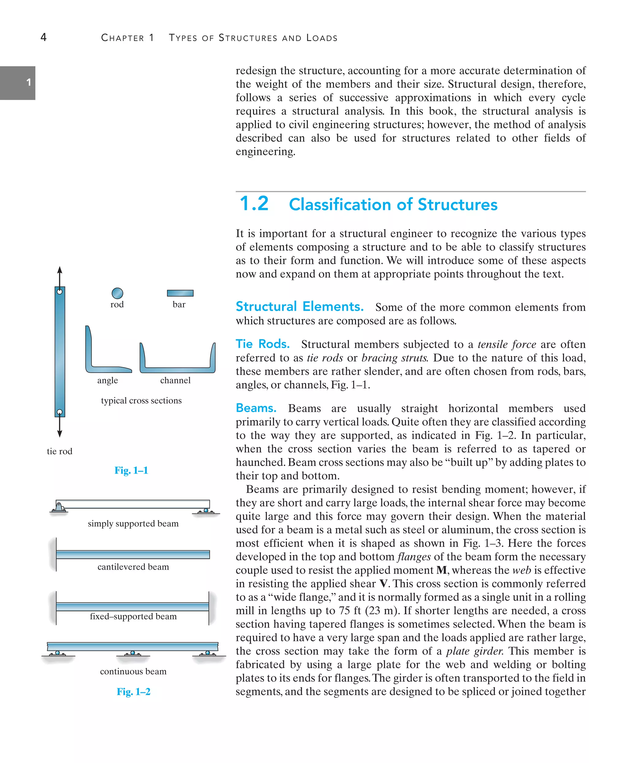
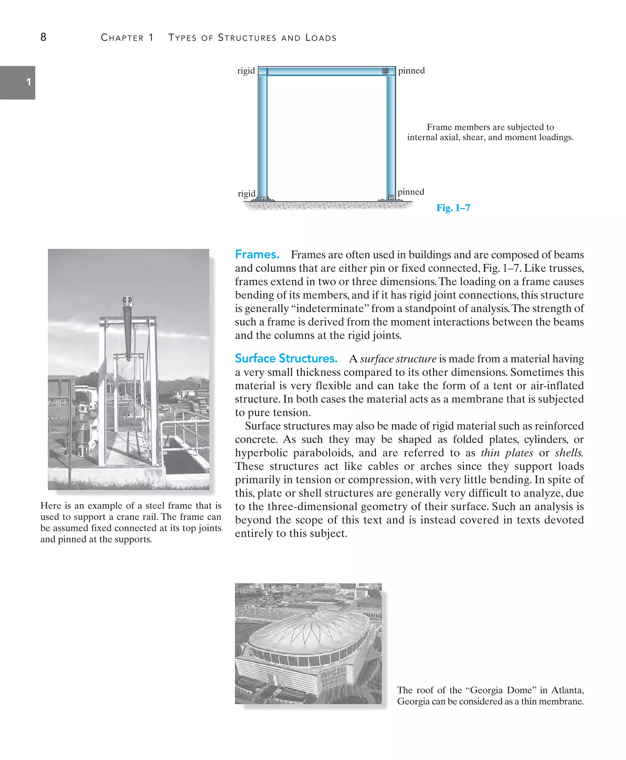
4 CHAPTER 1 TYPES OF STRUCTURES AND LOADS
1
redesign the structure, accounting for a more accurate determination of
the weight of the members and their size. Structural design, therefore,
follows a series of successive approximations in which every cycle
requires a structural analysis. In this book, the structural analysis is
applied to civil engineering structures; however, the method of analysis
described can also be used for structures related to other fields of
engineering.
1.2 Classification of Structures
It is important for a structural engineer to recognize the various types
of elements composing a structure and to be able to classify structures
as to their form and function. We will introduce some of these aspects
now and expand on them at appropriate points throughout the text.
Structural Elements. Some of the more common elements from
which structures are composed are as follows.
Tie Rods. Structural members subjected to a tensile force are often
referred to as tie rods or bracing struts. Due to the nature of this load,
these members are rather slender, and are often chosen from rods, bars,
angles, or channels, Fig. 1–1.
Beams. Beams are usually straight horizontal members used
primarily to carry vertical loads. Quite often they are classified according
to the way they are supported, as indicated in Fig. 1–2. In particular,
when the cross section varies the beam is referred to as tapered or
haunched. Beam cross sections may also be “built up” by adding plates to
their top and bottom.
Beams are primarily designed to resist bending moment; however, if
they are short and carry large loads, the internal shear force may become
quite large and this force may govern their design. When the material
used for a beam is a metal such as steel or aluminum, the cross section is
most efficient when it is shaped as shown in Fig. 1–3. Here the forces
developed in the top and bottom flanges of the beam form the necessary
couple used to resist the applied moment M, whereas the web is effective
in resisting the applied shear V. This cross section is commonly referred
to as a “wide flange,” and it is normally formed as a single unit in a rolling
mill in lengths up to 75 ft (23 m). If shorter lengths are needed, a cross
section having tapered flanges is sometimes selected. When the beam is
required to have a very large span and the loads applied are rather large,
the cross section may take the form of a plate girder. This member is
fabricated by using a large plate for the web and welding or bolting
plates to its ends for flanges.The girder is often transported to the field in
segments, and the segments are designed to be spliced or joined together
rod
tie rod
bar
angle channel
typical cross sections
Fig. 1–1
simply supported beam
cantilevered beam
fixed–supported beam
continuous beam
Fig. 1–2

1.2 CLASSIFICATION OF STRUCTURES 5
1
flange
flange
web
V
M
Fig. 1–3
at points where the girder carries a small internal moment. (See the
photo below.)
Concrete beams generally have rectangular cross sections, since it is
easy to construct this form directly in the field. Because concrete is
rather weak in resisting tension, steel “reinforcing rods” are cast into the
beam within regions of the cross section subjected to tension. Precast
concrete beams or girders are fabricated at a shop or yard in the same
manner and then transported to the job site.
Beams made from timber may be sawn from a solid piece of wood or
laminated. Laminated beams are constructed from solid sections of
wood, which are fastened together using high-strength glues.
The prestressed concrete girders are simply
supported and are used for this highway
bridge.
Shown are typical splice plate joints used
to connect the steel girders of a highway
bridge.
The steel reinforcement cage shown on the
right and left is used to resist any tension
that may develop in the concrete beams
which will be formed around it.

1
Columns. Members that are generally vertical and resist axial compressive
loads are referred to as columns, Fig. 1–4. Tubes and wide-flange cross
sections are often used for metal columns, and circular and square cross
sections with reinforcing rods are used for those made of concrete.
Occasionally, columns are subjected to both an axial load and a bending
moment as shown in the figure. These members are referred to as beam
columns.
Types of Structures. The combination of structural elements and
the materials from which they are composed is referred to as a structural
system. Each system is constructed of one or more of four basic types of
structures. Ranked in order of complexity of their force analysis, they are
as follows.
Trusses. When the span of a structure is required to be large and its
depth is not an important criterion for design, a truss may be selected.
Trusses consist of slender elements,usually arranged in triangular fashion.
Planar trusses are composed of members that lie in the same plane and
are frequently used for bridge and roof support, whereas space trusses have
members extending in three dimensions and are suitable for derricks
and towers.
Due to the geometric arrangement of its members, loads that cause the
entire truss to bend are converted into tensile or compressive forces in
the members. Because of this, one of the primary advantages of a truss,
compared to a beam, is that it uses less material to support a given load,
Fig. 1–5. Also, a truss is constructed from long and slender elements,
which can be arranged in various ways to support a load. Most often it is
Wide-flange members are often used for
columns. Here is an example of a beam
column.
beam column
column
Fig. 1–4

1.2 CLASSIFICATION OF STRUCTURES 7
1
economically feasible to use a truss to cover spans ranging from 30 ft
(9 m) to 400 ft (122 m), although trusses have been used on occasion for
spans of greater lengths.
Cables and Arches. Two other forms of structures used to span long
distances are the cable and the arch. Cables are usually flexible and carry
their loads in tension. They are commonly used to support bridges,
Fig. 1–6a, and building roofs. When used for these purposes, the cable has
an advantage over the beam and the truss, especially for spans that are
greater than 150 ft (46 m). Because they are always in tension, cables will
not become unstable and suddenly collapse, as may happen with beams or
trusses. Furthermore, the truss will require added costs for construction
and increased depth as the span increases. Use of cables, on the other
hand, is limited only by their sag, weight, and methods of anchorage.
The arch achieves its strength in compression, since it has a reverse
curvature to that of the cable. The arch must be rigid, however, in order
to maintain its shape, and this results in secondary loadings involving
shear and moment, which must be considered in its design. Arches are
frequently used in bridge structures, Fig. 1–6b, dome roofs, and for
openings in masonry walls.
Fig. 1–5
Fig. 1–6
Loading causes bending of truss,
which develops compression in top
members, tension in bottom
members.
Cables support their loads in tension.
(a)
Arches support their loads in compression.
(b)

1
Frames. Frames are often used in buildings and are composed of beams
and columns that are either pin or fixed connected, Fig. 1–7. Like trusses,
frames extend in two or three dimensions.The loading on a frame causes
bending of its members, and if it has rigid joint connections, this structure
is generally “indeterminate” from a standpoint of analysis.The strength of
such a frame is derived from the moment interactions between the beams
and the columns at the rigid joints.
Surface Structures. A surface structure is made from a material having
a very small thickness compared to its other dimensions. Sometimes this
material is very flexible and can take the form of a tent or air-inflated
structure. In both cases the material acts as a membrane that is subjected
to pure tension.
Surface structures may also be made of rigid material such as reinforced
concrete. As such they may be shaped as folded plates, cylinders, or
hyperbolic paraboloids, and are referred to as thin plates or shells.
These structures act like cables or arches since they support loads
primarily in tension or compression, with very little bending. In spite of
this, plate or shell structures are generally very difficult to analyze, due
to the three-dimensional geometry of their surface. Such an analysis is
beyond the scope of this text and is instead covered in texts devoted
entirely to this subject.
pinned
rigid
rigid pinned
Frame members are subjected to
internal axial, shear, and moment loadings.
Fig. 1–7
Here is an example of a steel frame that is
used to support a crane rail. The frame can
be assumed fixed connected at its top joints
and pinned at the supports.
The roof of the “Georgia Dome” in Atlanta,
Georgia can be considered as a thin membrane.

1.3 LOADS 9
1
1.3 Loads
Once the dimensional requirements for a structure have been defined,
it becomes necessary to determine the loads the structure must
support. Often, it is the anticipation of the various loads that will be
imposed on the structure that provides the basic type of structure that
will be chosen for design. For example, high-rise structures must
endure large lateral loadings caused by wind, and so shear walls and
tubular frame systems are selected, whereas buildings located in areas
prone to earthquakes must be designed having ductile frames and
connections.
Once the structural form has been determined, the actual design
begins with those elements that are subjected to the primary loads the
structure is intended to carry, and proceeds in sequence to the various
supporting members until the foundation is reached. Thus, a building
floor slab would be designed first, followed by the supporting beams,
columns, and last, the foundation footings. In order to design a structure,
it is therefore necessary to first specify the loads that act on it.
The design loading for a structure is often specified in codes. In general,
the structural engineer works with two types of codes: general building
codes and design codes.General building codes specify the requirements of
governmental bodies for minimum design loads on structures and
minimum standards for construction. Design codes provide detailed
technical standards and are used to establish the requirements for the
actual structural design.Table 1–1 lists some of the important codes used in
practice. It should be realized, however, that codes provide only a general
guide for design. The ultimate responsibility for the design lies with the
structural engineer.
TABLE 1–1 Codes
General Building Codes
Minimum Design Loads for Buildings and Other Structures,
ASCE/SEI 7-10,American Society of Civil Engineers
International Building Code
Design Codes
Building Code Requirements for Reinforced Concrete, Am. Conc. Inst. (ACI)
Manual of Steel Construction, American Institute of Steel Construction (AISC)
Standard Specifications for Highway Bridges, American Association of State
Highway and Transportation Officials (AASHTO)
National Design Specification for Wood Construction,American Forest and
Paper Association (AFPA)
Manual for Railway Engineering, American Railway Engineering
Association (AREA)

1
Since a structure is generally subjected to several types of loads, a brief
discussion of these loadings will now be presented to illustrate how one
must consider their effects in practice.
Dead Loads. Dead loads consist of the weights of the various
structural members and the weights of any objects that are permanently
attached to the structure. Hence, for a building, the dead loads include
the weights of the columns, beams, and girders, the floor slab, roofing,
walls, windows, plumbing, electrical fixtures, and other miscellaneous
attachments.
In some cases, a structural dead load can be estimated satisfactorily
from simple formulas based on the weights and sizes of similar
structures. Through experience one can also derive a “feeling” for the
magnitude of these loadings. For example, the average weight for timber
buildings is for steel framed buildings it is
and for reinforced concrete buildings it is
Ordinarily, though, once the materials
and sizes of the various components of the structure are determined,
their weights can be found from tables that list their densities.
The densities of typical materials used in construction are listed in
Table 1–2, and a portion of a table listing the weights of typical building
110–130 lb>ft2
15.3–6.2 kN>m2
2.
60–75 lb>ft2
12.9–3.6 kN>m2
2,
40–50 lb>ft2
11.9–2.4 kN>m2
2,
TABLE 1–2 Minimum Densities for Design Loads
from Materials*
lb兾ft3
kN兾m3
Aluminum 170 26.7
Concrete, plain cinder 108 17.0
Concrete, plain stone 144 22.6
Concrete, reinforced cinder 111 17.4
Concrete, reinforced stone 150 23.6
Clay, dry 63 9.9
Clay, damp 110 17.3
Sand and gravel, dry, loose 100 15.7
Sand and gravel, wet 120 18.9
Masonry, lightweight solid concrete 105 16.5
Masonry, normal weight 135 21.2
Plywood 36 5.7
Steel, cold-drawn 492 77.3
Wood, Douglas Fir 34 5.3
Wood, Southern Pine 37 5.8
Wood, spruce 29 4.5
*Reproduced with permission from American Society of Civil Engineers
Minimum Design Loads for Buildings and Other Structures, ASCE/SEI 7-10.
Copies of this standard may be purchased from ASCE at www.pubs.asce.org.

1.3 LOADS 11
1
components is given in Table 1–3. Although calculation of dead loads
based on the use of tabulated data is rather straightforward, it should be
realized that in many respects these loads will have to be estimated in
the initial phase of design. These estimates include nonstructural
materials such as prefabricated facade panels, electrical and plumbing
systems, etc. Furthermore, even if the material is specified, the unit
weights of elements reported in codes may vary from those given by
manufacturers, and later use of the building may include some changes
in dead loading.As a result, estimates of dead loadings can be in error by
15% to 20% or more.
Normally, the dead load is not large compared to the design load for
simple structures such as a beam or a single-story frame; however, for
multistory buildings it is important to have an accurate accounting of all
the dead loads in order to properly design the columns, especially for the
lower floors.
TABLE 1–3 Minimum Design Dead Loads*
Walls psf kN兾m2
4-in. (102 mm) clay brick 39 1.87
8-in. (203 mm) clay brick 79 3.78
12-in. (305 mm) clay brick 115 5.51
Frame Partitions and Walls
Exterior stud walls with brick veneer 48 2.30
Windows, glass, frame and sash 8 0.38
Wood studs unplastered 4 0.19
Wood studs plastered one side 12 0.57
Wood studs plastered two sides 20 0.96
Floor Fill
Cinder concrete, per inch (mm) 9 0.017
Lightweight concrete, plain, per inch (mm) 8 0.015
Stone concrete, per inch (mm) 12 0.023
Ceilings
Acoustical fiberboard 1 0.05
Plaster on tile or concrete 5 0.24
Suspended metal lath and gypsum plaster 10 0.48
Asphalt shingles 2 0.10
Fiberboard, (13 mm) 0.75 0.04
*Reproduced with permission from American Society of Civil Engineers Minimum Design Loads
for Buildings and Other Structures, ASCE/SEI 7-10.
1
2-in.
151 * 102 mm2
2 * 4 in.,
151 * 102 mm2
2 * 4 in.,
151 * 102 mm2
2 * 4 in.,

1
The live floor loading in this classroom
consists of desks, chairs and laboratory
equipment. For design the ASCE 7-10
Standard specifies a loading of 40 psf or
1.92 kN/m2
.
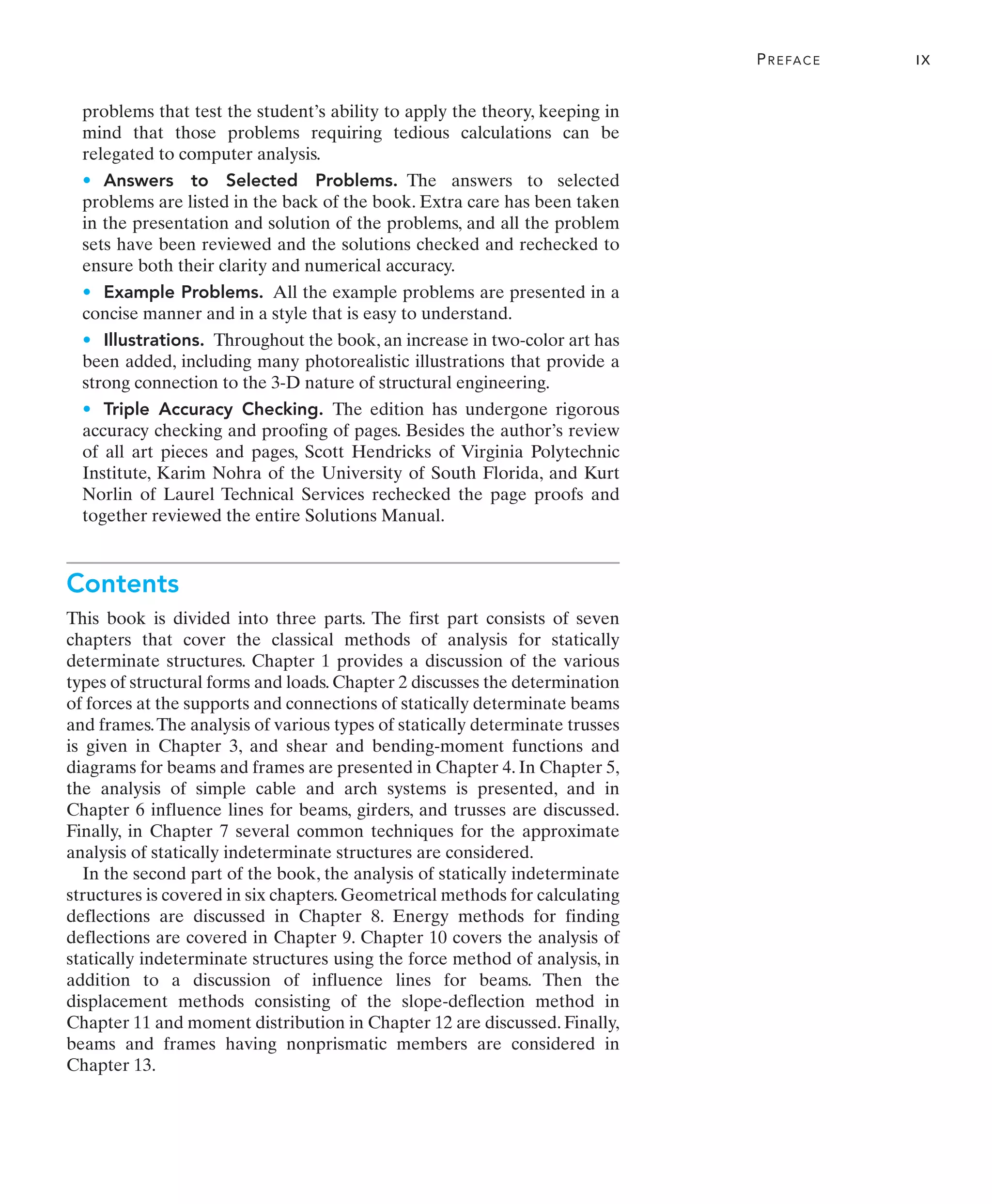
The floor beam in Fig. 1–8 is used to support the 6-ft width of a
lightweight plain concrete slab having a thickness of 4 in. The slab
serves as a portion of the ceiling for the floor below, and therefore its
bottom is coated with plaster. Furthermore, an 8-ft-high, 12-in.-thick
lightweight solid concrete block wall is directly over the top flange of
the beam. Determine the loading on the beam measured per foot of
length of the beam.
SOLUTION
Using the data in Tables 1–2 and 1–3, we have
Ans.
Here the unit k stands for “kip,” which symbolizes kilopounds. Hence,
1 k = 1000 lb.
Concrete slab:
Plaster ceiling:
Block wall:
Total load
[8 lb>1ft2 # in.2]14 in.216 ft2 = 192 lb>ft
15 lb>ft2
216 ft2 = 30 lb>ft
1105 lb>ft3
218 ft211 ft2 = 840 lb>ft
1062 lb>ft = 1.06 k>ft
EXAMPLE 1.1
3 ft
3 ft
8 ft
4 in.
12 in.
Fig. 1–8
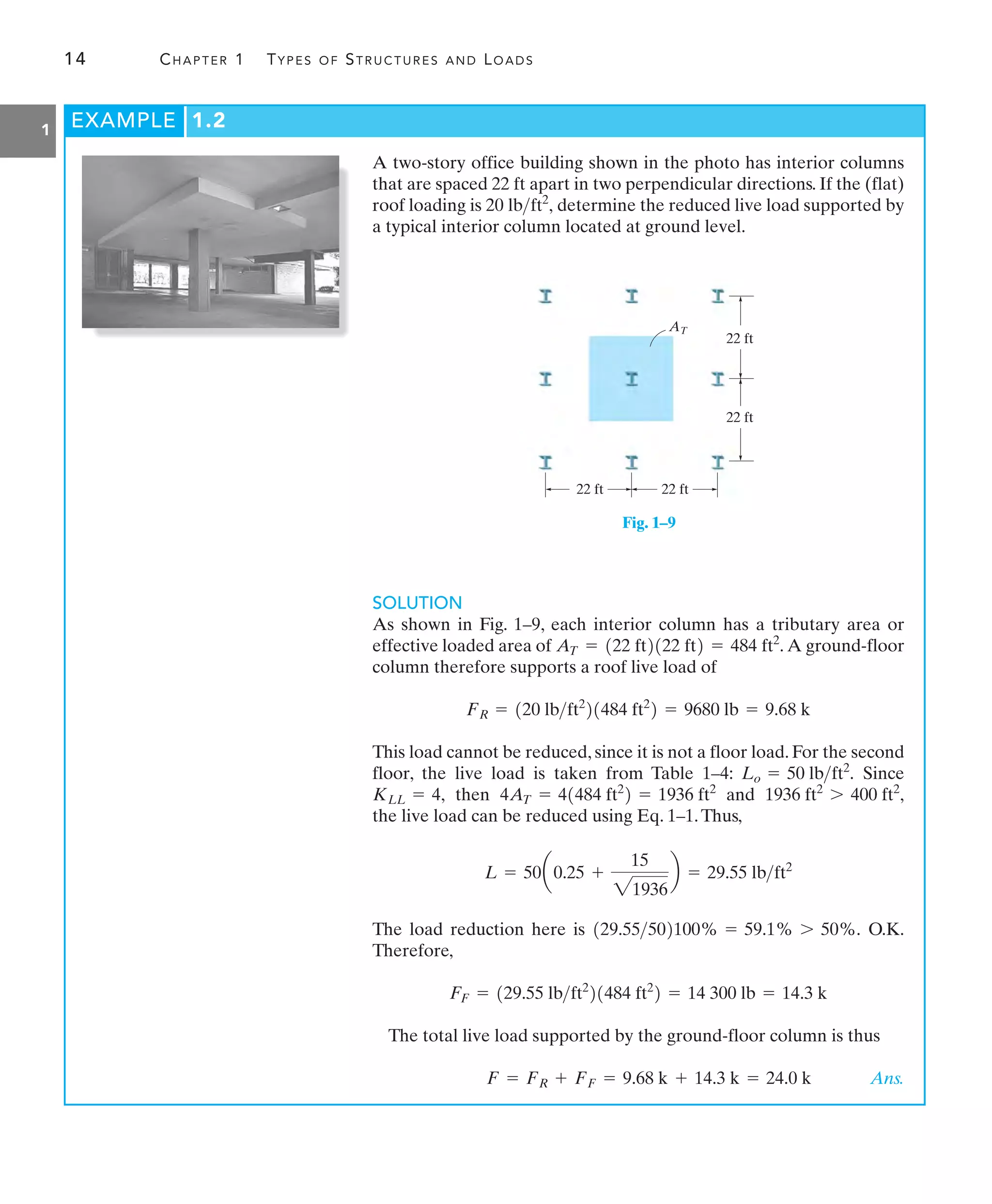
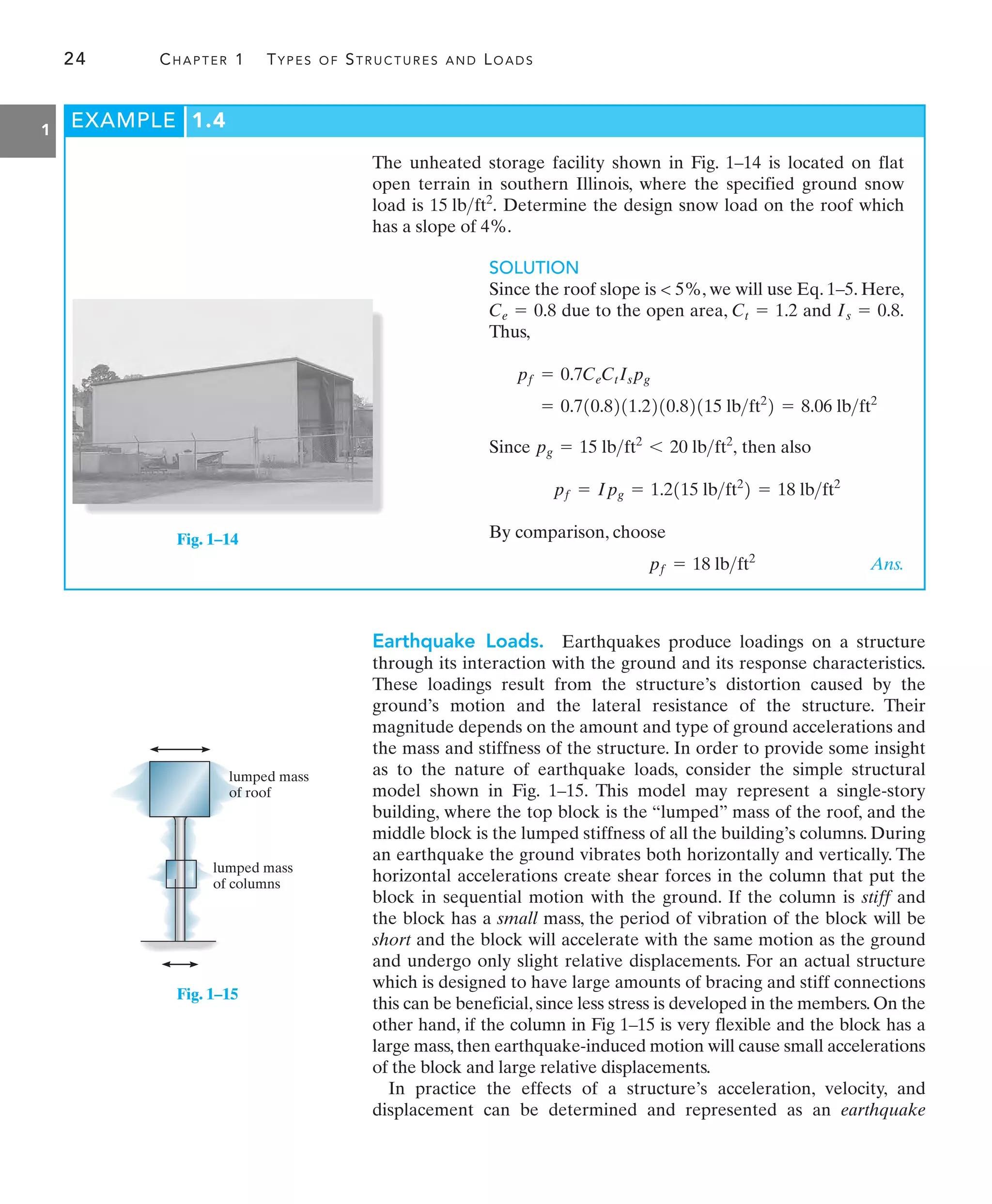
Live Loads. Live Loads can vary both in their magnitude and
location. They may be caused by the weights of objects temporarily
placed on a structure, moving vehicles, or natural forces. The minimum
live loads specified in codes are determined from studying the history
of their effects on existing structures. Usually, these loads include
additional protection against excessive deflection or sudden overload. In
Chapter 6 we will develop techniques for specifying the proper location
of live loads on the structure so that they cause the greatest stress or
deflection of the members. Various types of live loads will now be
discussed.
Building Loads. The floors of buildings are assumed to be subjected
to uniform live loads, which depend on the purpose for which the
building is designed. These loadings are generally tabulated in local,
state, or national codes. A representative sample of such minimum live
loadings, taken from the ASCE 7-10 Standard, is shown in Table 1–4.The
values are determined from a history of loading various buildings. They
include some protection against the possibility of overload due to
emergency situations, construction loads, and serviceability requirements
due to vibration. In addition to uniform loads, some codes specify
minimum concentrated live loads, caused by hand carts, automobiles, etc.,
which must also be applied anywhere to the floor system. For example,
both uniform and concentrated live loads must be considered in the
design of an automobile parking deck.

1.3 LOADS 13
1
For some types of buildings having very large floor areas, many codes
will allow a reduction in the uniform live load for a floor, since it is
unlikely that the prescribed live load will occur simultaneously throughout
the entire structure at any one time. For example, ASCE 7-10 allows a
reduction of live load on a member having an influence area of
or more. This reduced live load is calculated using the
following equation:
(1–1)
where
reduced design live load per square foot or square meter of area
supported by the member.
unreduced design live load per square foot or square meter of
area supported by the member (see Table 1–4).
live load element factor. For interior columns
tributary area in square feet or square meters.*
The reduced live load defined by Eq. 1–1 is limited to not less than 50%
of for members supporting one floor, or not less than 40% of for
members supporting more than one floor. No reduction is allowed for
loads exceeding or for structures used for public
assembly, garages, or roofs. Example 1–2 illustrates Eq. 1–1’s application.
100 lb>ft2
14.79 kN>m2
2,
Lo
Lo
AT =
KLL = 4.
KLL =
Lo =
L =
L = Loa0.25 +
4.57
2KLL AT
b 1SI units2
L = Loa0.25 +
15
2KLL AT
b 1FPS units2
400 ft2
137.2 m2
2
1KLL AT2
TABLE 1–4 Minimum Live Loads*
Live Load Live Load
Occupancy or Use psf kN兾m2
Occupancy or Use psf kN兾m2
Assembly areas and theaters Residential
Fixed seats 60 2.87 Dwellings (one- and two-family) 40 1.92
Movable seats 100 4.79 Hotels and multifamily houses
Garages (passenger cars only) 50 2.40 Private rooms and corridors 40 1.92
Office buildings Public rooms and corridors 100 4.79
Lobbies 100 4.79 Schools
Offices 50 2.40 Classrooms 40 1.92
Storage warehouse Corridors above first floor 80 3.83
Light 125 6.00
Heavy 250 11.97
*Reproduced with permission from Minimum Design Loads for Buildings and Other Structures,ASCE/SEI 7-10.
*Specific examples of the determination of tributary areas for beams and columns are
given in Sec. 2–1.

A two-story office building shown in the photo has interior columns
that are spaced 22 ft apart in two perpendicular directions. If the (flat)
roof loading is determine the reduced live load supported by
a typical interior column located at ground level.
20 lb>ft2
,
EXAMPLE 1.2
SOLUTION
As shown in Fig. 1–9, each interior column has a tributary area or
effective loaded area of A ground-floor
column therefore supports a roof live load of
This load cannot be reduced, since it is not a floor load. For the second
floor, the live load is taken from Table 1–4: Since
then and
the live load can be reduced using Eq. 1–1.Thus,
The load reduction here is O.K.
Therefore,
The total live load supported by the ground-floor column is thus
Ans.
F = FR + FF = 9.68 k + 14.3 k = 24.0 k
FF = 129.55 lb>ft2
21484 ft2
2 = 14 300 lb = 14.3 k
129.55>502100% = 59.1% 7 50%.
L = 50a0.25 +
15
21936
b = 29.55 lb>ft2
1936 ft2
7 400 ft2
,
4AT = 41484 ft2
2 = 1936 ft2
KLL = 4,
Lo = 50 lb>ft2
.
FR = 120 lb>ft2
21484 ft2
2 = 9680 lb = 9.68 k
AT = 122 ft2122 ft2 = 484 ft2
.
1
AT
22 ft
22 ft
22 ft
22 ft
Fig. 1–9

Highway Bridge Loads. The primary live loads on bridge spans are
those due to traffic, and the heaviest vehicle loading encountered is that
caused by a series of trucks. Specifications for truck loadings on highway
bridges are reported in the LRFD Bridge Design Specifications of the
American Association of State and Highway Transportation Officials
(AASHTO). For two-axle trucks, these loads are designated with an H,
followed by the weight of the truck in tons and another number which
gives the year of the specifications in which the load was reported.
H-series truck weights vary from 10 to 20 tons. However, bridges located
on major highways, which carry a great deal of traffic, are often designed
for two-axle trucks plus a one-axle semitrailer as in Fig. 1–10. These are
designated as HS loadings. In general, a truck loading selected for design
depends upon the type of bridge, its location, and the type of traffic
anticipated.
The size of the “standard truck” and the distribution of its weight is
also reported in the specifications.Although trucks are assumed to be on
the road, all lanes on the bridge need not be fully loaded with a row of
trucks to obtain the critical load, since such a loading would be highly
improbable.The details are discussed in Chapter 6.
Railroad Bridge Loads. The loadings on railroad bridges, as in
Fig. 1–11, are specified in the Specifications for Steel Railway Bridges
published by the American Railroad Engineers Association (AREA).
Normally, E loads, as originally devised by Theodore Cooper in 1894,
were used for design. B. Steinmann has since updated Cooper’s load
distribution and has devised a series of M loadings, which are currently
acceptable for design. Since train loadings involve a complicated series
of concentrated forces, to simplify hand calculations, tables and graphs
are sometimes used in conjunction with influence lines to obtain the
critical load.Also, computer programs are used for this purpose.
1.3 LOADS 15
1
Fig. 1–10
Fig. 1–11

1
Impact Loads. Moving vehicles may bounce or sidesway as they
move over a bridge, and therefore they impart an impact to the deck.The
percentage increase of the live loads due to impact is called the impact
factor, I.This factor is generally obtained from formulas developed from
experimental evidence. For example, for highway bridges the AASHTO
specifications require that
where L is the length of the span in feet that is subjected to the live
load.
In some cases provisions for impact loading on the structure of a
building must also be taken into account. For example, the ASCE 7-10
Standard requires the weight of elevator machinery to be increased by
100%, and the loads on any hangers used to support floors and balconies
to be increased by 33%.
Wind Loads. When structures block the flow of wind, the wind’s
kinetic energy is converted into potential energy of pressure, which
causes a wind loading. The effect of wind on a structure depends upon
the density and velocity of the air, the angle of incidence of the wind, the
shape and stiffness of the structure, and the roughness of its surface. For
design purposes, wind loadings can be treated using either a static or a
dynamic approach.
For the static approach, the fluctuating pressure caused by a constantly
blowing wind is approximated by a mean velocity pressure that acts on
the structure. This pressure q is defined by its kinetic energy,
where is the density of the air and V is its velocity. According to the
ASCE 7-10 Standard, this equation is modified to account for the
importance of the structure, its height, and the terrain in which it is
located. It is represented as
(1–2)
where
the velocity in miⲐh (m/s) of a 3-second gust of wind measured
33 ft (10 m) above the ground. Specific values depend upon
the “category” of the structure obtained from a wind map. For
V =
qz = 0.613KzKztKdV2
1N>m2
2
qz = 0.00256KzKztKdV2
1lb>ft2
2
r
q = 1
2 rV2
,
I =
50
L + 125
but not larger than 0.3

1.3 LOADS 17
1
example, the interior portion of the continental United States
reports a wind speed of 105 mi/h (47 m/s) if the structure
is an agricultural or storage building, since it is of low risk to
human life in the event of a failure. The wind speed is 120 mi/h
(54 m/s) for cases where the structure is a hospital, since its
failure would cause substantial loss of human life.
the velocity pressure exposure coefficient, which is a function
of height and depends upon the ground terrain.Table 1–5 lists
values for a structure which is located in open terrain with
scattered low-lying obstructions.
a factor that accounts for wind speed increases due to hills and
escarpments. For flat ground
a factor that accounts for the direction of the wind. It is used only
when the structure is subjected to combinations of loads (see
Sec. 1–4). For wind acting alone, Kd = 1.0.
Kd =
Kzt = 1.0.
Kzt =
Kz =
Hurricane winds caused this damage to a condominium in
Miami, Florida.
TABLE 1–5 Velocity Pressure
Exposure Coefficient for Terrain with
Low-Lying Obstructions
z
ft m Kz
0–15 0–4.6 0.85
20 6.1 0.90
25 7.6 0.94
30 9.1 0.98
40 12.2 1.04
50 15.2 1.09

1
Design Wind Pressure for Enclosed Buildings. Once the value for
is obtained, the design pressure can be determined from a list of
relevant equations listed in the ASCE 7-10 Standard. The choice
depends upon the flexibility and height of the structure, and whether
the design is for the main wind-force resisting system, or for the
building’s components and cladding. For example, using a “directional
procedure” the wind-pressure on an enclosed building of any height is
determined using a two-termed equation resulting from both external
and internal pressures, namely,
(1–3)
Here
for the windward wall at height z above the ground
(Eq. 1–2), and for the leeward walls, side walls,
and roof, where the mean height of the roof.
a wind-gust effect factor, which depends upon the exposure.
For example, for a rigid structure,
a wall or roof pressure coefficient determined from a
table. These tabular values for the walls and a roof pitch of
are given in Fig. 1–12. Note in the elevation view
that the pressure will vary with height on the windward
side of the building, whereas on the remaining sides and
on the roof the pressure is assumed to be constant.
Negative values indicate pressures acting away from the
surface.
the internal pressure coefficient, which depends upon the
type of openings in the building. For fully enclosed
buildings Here the signs indicate that
either positive or negative (suction) pressure can occur
within the building.
Application of Eq. 1–3 will involve calculations of wind pressures from
each side of the building, with due considerations for the possibility of
either positive or negative pressures acting on the building’s interior.
1GCpi2 = ;0.18.
1GCpi2 =
u = 10°
Cp =
G = 0.85.
G =
z = h,
q = qh
qz
q =
p = qGCp - qh1GCpi2
qz
Wind blowing on a wall will tend to tip a
building or cause it to sidesway. To prevent
this engineers often use cross bracing to
provide stability.Also, see p. 46.

1.3 LOADS 19
1
For high-rise buildings or those having a shape or location that makes
them wind sensitive, it is recommended that a dynamic approach be used
to determine the wind loadings. The methodology for doing this is also
outlined in the ASCE 7-10 Standard. It requires wind-tunnel tests to be
performed on a scale model of the building and those surrounding it, in
order to simulate the natural environment. The pressure effects of the
wind on the building can be determined from pressure transducers
attached to the model.Also, if the model has stiffness characteristics that
are in proper scale to the building, then the dynamic deflections of the
building can be determined.
Fig. 1–12
B
L
wind
qhGCp
qhGCp
qzGCp
qhGCp
ridge
plan
L
h
z
qhGCp qhGCp
qhGCp
qzGCp
elevation
u
Surface Use with
All values
All values
Wall pressure coefficients, Cp
(a)
Side walls
Windward
wall
Leeward
wall
L/B
01
2
4
Cp
qz
qh
qh
0.8
0.5
0.3
0.2
0.7
Maximum negative roof pressure
coefficients, Cp, for use with qh
Wind
direction
Normal to
ridge
h/L 10 u 10
Leeward
angle
Windward
angle u
0.7
0.9
1.3
0.3
0.5
0.7
0.25
0.5
1.0
(b)

The enclosed building shown in the photo and in Fig. 1–13a is used for
storage purposes and is located outside of Chicago, Illinois on open
flat terrain.When the wind is directed as shown, determine the design
wind pressure acting on the roof and sides of the building using the
ASCE 7-10 Specifications.
SOLUTION
First the wind pressure will be determined using Eq. 1–2. The basic
wind speed is since the building is used for storage.
Also, for flat terrain, . Since only wind loading is being
considered, . Therefore,
From Fig. 1–13a, so that the mean height
of the roof is Using the values of in
Table 1–5,calculated values of the pressure profile are listed in the table
in Fig. 1–13b. Note the value of was determined by linear interpola-
tion for i.e.,
and so
In order to apply Eq. 1–3 the gust factor is and
Thus,
(1)
The pressure loadings are obtained from this equation using the
calculated values for listed in Fig. 1–13b in accordance with the
wind-pressure profile in Fig. 1–12.
qz
= 0.85qCp 5.03
= q10.852Cp - 27.91;0.182
p = qGCp - qh1GCpi2
;0.18.
1GCpi2 =
G = 0.85,
qh = 28.2210.9902 = 27.9 psf.
Kz = 0.990,
11.04 - 0.982140 - 302 = 11.04 - Kz2140 - 31.62,
z = h,
Kz
Kz
h = 25 + 13.222 = 31.6 ft.
h¿ = 75 tan 10° = 13.22 ft
= 28.22 Kz
= 0.00256 Kz11.0211.02110522
qz = 0.00256 KzKztKdV2
Kd = 1.0
Kzt = 1.0
V = 105 mih,
EXAMPLE 1.3
1
Fig. 1–13
z (ft) Kz qz (psf)
0–15 0.85 24.0
20 0.90 25.4
25 0.94 26.5
0.990 27.9
h = 31.6
(b)
150 ft
wind
75 ft
75 ft
25 ft
h
h
(a)
10 h
10

1.3 LOADS 21
1
Windward Wall. Here the pressure varies with height z since
must be used. For all values of , so that from Eq. (1),
Leeward Wall. Here so that
Also, and so from Eq. (1),
Side Walls. For all values of , and therefore since
we must use in Eq. (1), we have
Windward Roof. Here so that
and Thus,
Leeward Roof. In this case therefore with we get
These two sets of loadings are shown on the elevation of the building,
representing either positive or negative (suction) internal building
pressure, Fig. 1–13c. The main framing structure of the building must
resist these loadings as well as for separate loadings calculated from
wind blowing on the front or rear of the building.
p = -12.2 psf or -2.09 psf
q = qh,
Cp = -0.3;
p = -21.6 psf or -11.6 psf
q = qh.
Cp = -0.7
hL = 31.621752 = 0.211 6 0.25,
p = -21.6 psf or -11.6 psf
q = qh
Cp = -0.7,
LB
p = -16.9 psf or -6.84 psf
q = qh
Cp = -0.5.
LB = 21752150 = 1,
p25 = 13.0 psf or 23.1 psf
p20 = 12.2 psf or 22.3 psf
p0-15 = 11.3 psf or 21.3 psf
Cp = 0.8,
LB
qzGCp
11.3 psf
12.2 psf
13.0 psf
21.6 psf
12.2 psf
16.9 psf
(c)
21.3 psf
22.3 psf
23.1 psf
11.6 psf
2.09 psf
6.84 psf

1
Design Wind Pressure for Signs. If the structure represents a sign, the
wind will produce a resultant force acting on the face of the sign which is
determined from
(1–4)
Here
the wind pressure evaluated at the height h, measured from the
ground to the top of the sign.
the wind-gust coefficient factor defined previously.
a force coefficient which depends upon the aspect ratio (width B of
the sign to height s of the sign), and the clear area ratio (sign height
s to the elevation h, measured from the ground to the top of the
sign). For cases of wind directed normal to the sign and through its
center, for , values are listed in Table 1–6.
the area of the face of the sign in ft2
(m2
).
As =
Bs = 4
Cf =
G =
qh =
F = qhGCfAs
Hurricane winds acting on the face of this
sign were strong enough to noticeably
bend the two supporting arms causing the
material to yield. Proper design would
have prevented this.
TABLE 1–6 Force Coefficients for
Above-Ground Solid Signs, Cf
s兾h Cf
1.35
0.9 1.45
0.5 1.70
0.2 1.80
1.85
…0.16
1
To allow for normal and oblique wind directions, the calculated
resultant force is assumed to act either through the geometric center of
the face of the sign or at other specified locations on the face of the sign
which depend upon the ratios s兾h and B兾s.

1.3 LOADS 23
1
Snow Loads. In some parts of the country, roof loading due to snow
can be quite severe, and therefore protection against possible failure is of
primary concern. Design loadings typically depend on the building’s
general shape and roof geometry, wind exposure, location, its
importance, and whether or not it is heated. Like wind, snow loads in
the ASCE 7-10 Standard are generally determined from a zone map
reporting 50-year recurrence intervals of an extreme snow depth. For
example, on the relatively flat elevation throughout the mid-section of
Illinois and Indiana, the ground snow loading is
However, for areas of Montana, specific case studies of ground snow
loadings are needed due to the variable elevations throughout the state.
Specifications for snow loads are covered in the ASCE 7-10 Standard,
although no single code can cover all the implications of this type of
loading.
If a roof is flat, defined as having a slope of less than 5%, then the
pressure loading on the roof can be obtained by modifying the ground
snow loading, by the following empirical formula
(1–5)
Here
an exposure factor which depends upon the terrain. For example,
for a fully exposed roof in an unobstructed area,
whereas if the roof is sheltered and located in the center of a large
city, then
a thermal factor which refers to the average temperature within
the building. For unheated structures kept below freezing
whereas if the roof is supporting a normally heated
structure, then
the importance factor as it relates to occupancy. For example,
for agriculture and storage facilities, and for
schools and hospitals.
If then use the largest value for either
computed from the above equation or from If
then use pf = Is120 lbft2
2.
10.96 kNm2
2,
pg 7 20 lbft2
pf = Ispg.
pf,
pg … 20 lbft2
10.96 kNm2
2,
Is = 1.20
Is = 0.80
Is =
Ct = 1.0.
Ct = 1.2,
Ct =
Ce = 1.2.
Ce = 0.8,
Ce =
pf = 0.7CeCtIspg
pg,
20 lbft2
10.96 kNm2
2.
Excessive snow and ice loadings act on this
roof.

1
Earthquake Loads. Earthquakes produce loadings on a structure
through its interaction with the ground and its response characteristics.
These loadings result from the structure’s distortion caused by the
ground’s motion and the lateral resistance of the structure. Their
magnitude depends on the amount and type of ground accelerations and
the mass and stiffness of the structure. In order to provide some insight
as to the nature of earthquake loads, consider the simple structural
model shown in Fig. 1–15. This model may represent a single-story
building, where the top block is the “lumped” mass of the roof, and the
middle block is the lumped stiffness of all the building’s columns. During
an earthquake the ground vibrates both horizontally and vertically. The
horizontal accelerations create shear forces in the column that put the
block in sequential motion with the ground. If the column is stiff and
the block has a small mass, the period of vibration of the block will be
short and the block will accelerate with the same motion as the ground
and undergo only slight relative displacements. For an actual structure
which is designed to have large amounts of bracing and stiff connections
this can be beneficial, since less stress is developed in the members. On the
other hand, if the column in Fig 1–15 is very flexible and the block has a
large mass, then earthquake-induced motion will cause small accelerations
of the block and large relative displacements.
In practice the effects of a structure’s acceleration, velocity, and
displacement can be determined and represented as an earthquake
The unheated storage facility shown in Fig. 1–14 is located on flat
open terrain in southern Illinois, where the specified ground snow
load is Determine the design snow load on the roof which
has a slope of 4%.
15 lbft2
.
EXAMPLE 1.4
Fig. 1–14
SOLUTION
Since the roof slope is 5%, we will use Eq. 1–5. Here,
due to the open area, and
Thus,
Since then also
By comparison, choose
Ans.
pf = 18 lbft2
pf = Ipg = 1.2115 lbft2
2 = 18 lbft2
pg = 15 lbft2
6 20 lbft2
,
= 0.710.8211.2210.82115 lbft2
2 = 8.06 lbft2
pf = 0.7CeCtIspg
Is = 0.8.
Ct = 1.2
Ce = 0.8
lumped mass
of columns
lumped mass
of roof
Fig. 1–15

1.3 LOADS 25
1
response spectrum. Once this graph is established, the earthquake
loadings can be calculated using a dynamic analysis based on the theory
of structural dynamics. This type of analysis is gaining popularity,
although it is often quite elaborate and requires the use of a computer.
Even so, such an analysis becomes mandatory if the structure is large.
Some codes require that specific attention be given to earthquake
design, especially in areas of the country where strong earthquakes
predominate. Also, these loads should be seriously considered when
designing high-rise buildings or nuclear power plants. In order to assess
the importance of earthquake design consideration, one can check the
seismic ground-acceleration maps published in the ASCE 7-10 Standard.
These maps provide the peak ground accelerations caused by an
earthquake along with risk coefficients. Regions vary from low risk, such
as parts of Texas, to very high risk, such as along the west coast of
California.
For small structures, a static analysis for earthquake design may be
satisfactory. This case approximates the dynamic loads by a set of
externally applied static forces that are applied laterally to the structure.
One such method for doing this is reported in the ASCE 7-10 Standard.
It is based upon finding a seismic response coefficient, , determined
from the soil properties, the ground accelerations, and the vibrational
response of the structure. For most structures, this coefficient is then
multiplied by the structure’s total dead load W to obtain the “base shear”
in the structure.The value of is actually determined from
where
the spectral response acceleration for short periods of vibration.
a response modification factor that depends upon the ductility of
the structure. Steel frame members which are highly ductile can
have a value as high as 8, whereas reinforced concrete frames
can have a value as low as 3.
the importance factor that depends upon the use of the building.
For example, for agriculture and storage facilities, and
for hospitals and other essential facilities.
With each new publication of the Standard, values of these coefficients
are updated as more accurate data about earthquake response become
available.
Hydrostatic and Soil Pressure. When structures are used to retain
water, soil, or granular materials, the pressure developed by these
loadings becomes an important criterion for their design. Examples of
such types of structures include tanks, dams, ships, bulkheads, and
retaining walls. Here the laws of hydrostatics and soil mechanics are
applied to define the intensity of the loadings on the structure.
Ie = 1.5
Ie = 1
Ie =
R =
SDS =
Cs =
SDS
RIe
Cs
Cs
The design of this retaining wall requires
estimating the soil pressure acting on it.
Also, the gate of the lock will be subjected
to hydrostatic pressure that must be
considered for its design.

1
Other Natural Loads. Several other types of live loads may also
have to be considered in the design of a structure, depending on its
location or use. These include the effect of blast, temperature changes,
and differential settlement of the foundation.
1.4 Structural Design
Whenever a structure is designed, it is important to give consideration
to both material and load uncertainties. These uncertainties include a
possible variability in material properties, residual stress in materials,
intended measurements being different from fabricated sizes, loadings
due to vibration or impact, and material corrosion or decay.
ASD. Allowable-stress design (ASD) methods include both the
material and load uncertainties into a single factor of safety. The many
types of loads discussed previously can occur simultaneously on a
structure, but it is very unlikely that the maximum of all these loads will
occur at the same time. For example, both maximum wind and
earthquake loads normally do not act simultaneously on a structure. For
allowable-stress design the computed elastic stress in the material must
not exceed the allowable stress for each of various load combinations.
Typical load combinations as specified by the ASCE 7-10 Standard
include
• dead load
•
•
LRFD. Since uncertainty can be considered using probability theory,
there has been an increasing trend to separate material uncertainty from
load uncertainty. This method is called strength design or LRFD (load
and resistance factor design). For example, to account for the uncertainty
of loads, this method uses load factors applied to the loads or
combinations of loads. According to the ASCE 7-10 Standard, some of
the load factors and combinations are
• 1.4 (dead load)
•
• 0.9 (dead load) 1.0 (wind load)
• 0.9 (dead load) 1.0 (earthquake load)
In all these cases, the combination of loads is thought to provide a
maximum, yet realistic loading on the structure.
+
+
1.2 1dead load2 + 1.6 1live load2 + 0.5 1snow load2
0.6 1dead load2 + 0.7 1earthquake load2
0.6 1dead load2 + 0.6 (wind load)

1.4 STRUCTURAL DESIGN 27
1
1–1. The floor of a heavy storage warehouse building is
made of 6-in.-thick stone concrete. If the floor is a slab
having a length of 15 ft and width of 10 ft, determine the
resultant force caused by the dead load and the live load.
1–2. The floor of the office building is made of 4-in.-thick
lightweight concrete. If the office floor is a slab having a
length of 20 ft and width of 15 ft, determine the resultant
force caused by the dead load and the live load.
*1–4. The “New Jersey” barrier is commonly used during
highway construction. Determine its weight per foot of
length if it is made from plain stone concrete.
PROBLEMS
Prob. 1–2
26 in.
40 in.
8 in.
10 in.
Prob. 1–3
12 in.
4 in.
24 in.
6 in.
55°
75°
Prob. 1–4
1–3. The T-beam is made from concrete having a specific
weight of 150 lb/ft3
. Determine the dead load per foot length
of beam. Neglect the weight of the steel reinforcement.
1–5. The floor of a light storage warehouse is made of
150-mm-thick lightweight plain concrete. If the floor is a
slab having a length of 7 m and width of 3 m, determine the
resultant force caused by the dead load and the live load.
1–6. The prestressed concrete girder is made from plain
stone concrete and four -in. cold-form steel reinforcing
rods. Determine the dead weight of the girder per foot of its
length.
3
4
8 in.
8 in.
4 in.
4 in.
6 in.
6 in.
6 in.
20 in.
Prob. 1–6

1
2.5 m
Prob. 1–7
1–7. The wall is 2.5 m high and consists of 51 mm ×
102 mm studs plastered on one side. On the other side is
13 mm fiberboard, and 102 mm clay brick. Determine the
average load in kN/m of length of wall that the wall exerts
on the floor.
1–11. A four-story office building has interior columns
spaced 30 ft apart in two perpendicular directions. If the
flat-roof live loading is estimated to be 30 lb/ft2
, determine
the reduced live load supported by a typical interior column
located at ground level.
*1–12. A two-story light storage warehouse has interior
columns that are spaced 12 ft apart in two perpendicular
directions. If the live loading on the roof is estimated to be
25 lb/ft2
, determine the reduced live load supported by a
typical interior column at (a) the ground-floor level, and (b)
the second-floor level.
1–13. The office building has interior columns spaced 5 m
apart in perpendicular directions. Determine the reduced
live load supported by a typical interior column located on
the first floor under the offices.
*1–8. A building wall consists of exterior stud walls with
brick veneer and 13 mm fiberboard on one side. If the wall
is 4 m high, determine the load in kN/m that it exerts on the
floor.
1–9. The interior wall of a building is made from 2 × 4
wood studs, plastered on two sides. If the wall is 12 ft high,
determine the load in lb/ft of length of wall that it exerts on
the floor.
1–10. The second floor of a light manufacturing building is
constructed from a 5-in.-thick stone concrete slab with an
added 4-in. cinder concrete fill as shown. If the suspended
ceiling of the first floor consists of metal lath and gypsum
plaster, determine the dead load for design in pounds per
square foot of floor area.
1–14. A two-story hotel has interior columns for the
rooms that are spaced 6 m apart in two perpendicular
directions. Determine the reduced live load supported by a
typical interior column on the first floor under the public
rooms.
4 in. cinder fill
5 in. concrete slab
ceiling
Prob. 1–10
Prob. 1–13

Prob. 1–16
Prob. 1–15
1.4 STRUCTURAL DESIGN 29
1
1–15. Wind blows on the side of a fully enclosed hospital
located on open flat terrain in Arizona. Determine the
external pressure acting over the windward wall, which has
a height of 30 ft.The roof is flat.
*1–16. Wind blows on the side of the fully enclosed
hospital located on open flat terrain in Arizona. Determine
the external pressure acting on the leeward wall, which has
a length of 200 ft and a height of 30 ft.
1–18. The light metal storage building is on open flat
terrain in central Oklahoma. If the side wall of the building
is 14 ft high, what are the two values of the external wind
pressure acting on this wall when the wind blows on the
back of the building? The roof is essentially flat and the
building is fully enclosed.
1–17. A closed storage building is located on open flat
terrain in central Ohio. If the side wall of the building is
20 ft high, determine the external wind pressure acting on
the windward and leeward walls. Each wall is 60 ft long.
Assume the roof is essentially flat.
Prob. 1–17
Prob. 1–18

1
*1–20. A hospital located in central Illinois has a flat roof.
Determine the snow load in kN/m2
that is required to
design the roof.
1–19. Determine the resultant force acting perpendicular
to the face of the billboard and through its center if it is
located in Michigan on open flat terrain. The sign is rigid
and has a width of 12 m and a height of 3 m. Its top side is
15 m from the ground.
Prob. 1–19
1–21. The school building has a flat roof. It is located in an
open area where the ground snow load is 0.68 kN/m2
.
Determine the snow load that is required to design the roof.
1–22. The hospital is located in an open area and has a
flat roof and the ground snow load is 30 lb/ft2
. Determine
the design snow load for the roof.
Prob. 1–21
Prob. 1–22

CHAPTER REVIEW 31
1
The basic structural elements are:
Tie Rods—Slender members subjected to tension. Often used for bracing.
Beams—Members designed to resist bending moment. They are often fixed or pin supported and can be in the form of a
steel plate girder, reinforced concrete, or laminated wood.
Columns—Members that resist axial compressive force. If the column also resists bending, it is called a beam column.
tie rod
beam column
column
simply supported beam
cantilevered beam
Loads are specified in codes such as the ASCE 7-10
code. Dead loads are fixed and refer to the weights of
members and materials. Live loads are movable
and consist of uniform building floor loads, traffic and
train loads on bridges, impact loads due to vehicles
and machines, wind loads, snow loads, earthquake
loads, and hydrostatic and soil pressure.
The types of structures considered in this book consist of trusses made from slender pin-connected members forming a
series of triangles, cables and arches, which carry tensile and compressive loads, respectively, and frames composed of
pin- or fixed-connected beams and columns.
CHAPTER REVIEW

Oftentimes the elements of a structure, like the beams and girders of this
building frame, are connected together in a manner whereby the analysis can
be considered statically determinate.

2
33
In this chapter we will direct our attention to the most common form
of structure that the engineer will have to analyze, and that is one
that lies in a plane and is subjected to a force system that lies in the
same plane. We begin by discussing the importance of choosing an
appropriate analytical model for a structure so that the forces in the
structure may be determined with reasonable accuracy. Then the criteria
necessary for structural stability are discussed. Finally, the analysis of
statically determinate, planar, pin-connected structures is presented.
2.1 Idealized Structure
An exact analysis of a structure can never be carried out, since estimates
always have to be made of the loadings and the strength of the
materials composing the structure. Furthermore, points of application
for the loadings must also be estimated. It is important, therefore,
that the structural engineer develop the ability to model or idealize a
structure so that he or she can perform a practical force analysis of the
members. In this section we will develop the basic techniques necessary
to do this.
Determinate Structures

34 CHAPTER 2 ANALYSIS OF STATICALLY DETERMINATE STRUCTURES
Fig. 2–2
2
Notice that the deck of this concrete bridge is
made so that one section can be considered
roller supported on the other section.
Support Connections. Structural members are joined together in
various ways depending on the intent of the designer.The three types of
joints most often specified are the pin connection, the roller support, and
the fixed joint. A pin-connected joint and a roller support allow some
freedom for slight rotation,whereas a fixed joint allows no relative rotation
between the connected members and is consequently more expensive to
fabricate. Examples of these joints, fashioned in metal and concrete, are
shown in Figs. 2–1 and 2–2, respectively. For most timber structures, the
members are assumed to be pin connected, since bolting or nailing them
will not sufficiently restrain them from rotating with respect to each other.
Idealized models used in structural analysis that represent pinned and
fixed supports and pin-connected and fixed-connected joints are shown
in Figs. 2–3a and 2–3b. In reality, however, all connections exhibit some
stiffness toward joint rotations, owing to friction and material behavior.
In this case a more appropriate model for a support or joint might be
that shown in Fig. 2–3c. If the torsional spring constant the joint is
a pin, and if the joint is fixed.
k : q,
k = 0,
Fig. 2–1
weld
weld
stiffeners
(b)
typical “fixed-supported” connection (concrete)
(a)
typical “pin-supported” connection (metal)
(a)
typical “roller-supported” connection (concrete)
(b)
typical “fixed-supported” connection (metal)

2.1 IDEALIZED STRUCTURE 35
2
Fig. 2–4
Fig. 2–3
When selecting a particular model for each support or joint, the engineer
must be aware of how the assumptions will affect the actual performance
of the member and whether the assumptions are reasonable for the
structural design. For example, consider the beam shown in Fig. 2–4a,
which is used to support a concentrated load P. The angle connection at
support A is like that in Fig. 2–1a and can therefore be idealized as a
typical pin support.Furthermore,the support at B provides an approximate
point of smooth contact and so it can be idealized as a roller.The beam’s
thickness can be neglected since it is small in comparison to the beam’s
length, and therefore the idealized model of the beam is as shown in
Fig. 2–4b.The analysis of the loadings in this beam should give results that
closely approximate the loadings in the actual beam.To show that the model
is appropriate,consider a specific case of a beam made of steel with
(8000 lb) and One of the major simplifications made here was
assuming the support at A to be a pin. Design of the beam using standard
code procedures* indicates that a W would be adequate for
supporting the load. Using one of the deflection methods of Chapter 8, the
rotation at the “pin” support can be calculated as
From Fig. 2–4c, such a rotation only moves the top or bottom flange a
distance of This small
amount would certainly be accommodated by the connection fabricated as
shown in Fig. 2–1a, and therefore the pin serves as an appropriate model.
¢ = ur = 10.0103 rad215.12 in.2 = 0.0528 in.!
u = 0.0103 rad = 0.59°.
10 * 19
L = 20 ft.
P = 8 k
*Codes such as the Manual of Steel Construction, American Institute of Steel Construction.
pin support pin-connected joint
(a)
fixed support
(b)
fixed-connected joint
torsional spring support torsional spring joint
(c)
k k
L
––
2
L
––
2
A
B
P
actual beam
(a)
L
––
2
L
––
2
P
B
A
idealized beam
(b) (c)
5.12 in.
5.12 in.
0.59
0.0528 in.
0.0528 in.
0.59

2
Other types of connections most commonly encountered on coplanar
structures are given in Table 2–1. It is important to be able to recognize
the symbols for these connections and the kinds of reactions they exert
on their attached members. This can easily be done by noting how the
connection prevents any degree of freedom or displacement of the
member. In particular, the support will develop a force on the member if
it prevents translation of the member, and it will develop a moment if it
prevents rotation of the member. For example, a member in contact
with a smooth surface (3) is prevented from translating only in one
direction, which is perpendicular or normal to the surface. Hence, the
surface exerts only a normal force F on the member in this direction.
The magnitude of this force represents one unknown.Also note that the
member is free to rotate on the surface, so that a moment cannot be
developed by the surface on the member.As another example, the fixed
support (7) prevents both translation and rotation of a member at the
point of connection. Therefore, this type of support exerts two force
components and a moment on the member. The “curl” of the moment
lies in the plane of the page, since rotation is prevented in that plane.
Hence, there are three unknowns at a fixed support.
In reality, all supports actually exert distributed surface loads on their
contacting members. The concentrated forces and moments shown in
Table 2–1 represent the resultants of these load distributions. This
representation is, of course, an idealization; however, it is used here since
the surface area over which the distributed load acts is considerably
smaller than the total surface area of the connecting members.
A typical rocker support used for a bridge
girder.
Rollers and associated bearing pads are
used to support the prestressed concrete
girders of a highway bridge.
The short link is used to connect the two
girders of the highway bridge and allow
for thermal expansion of the deck.
Typical pin used to support the steel
girder of a railroad bridge.

2
TABLE 2–1 Supports for Coplanar Structures
Type of Connection Idealized Symbol Reaction Number of Unknowns
(4)
smooth pin-connected collar
F
(1) light cable
U
weightless link
F
U
(2)
rollers
rocker
F
(3)
smooth contacting surface
F
(5)
smooth pin or hinge
U Fy
Fx
U
Fx
(7)
fixed support
Fy
M
One unknown. The reaction is a
force that acts in the direction
of the cable or link.
force that acts perpendicular to
the surface at the point of contact.
Two unknowns. The reactions are
two force components.
Two unknowns. The reactions
are a force and a moment.
Three unknowns. The reactions are
the moment and the two force
components.
fixed-connected collar
(6)
slider
F
M
U
U

Fig. 2–6
(a)
D
A
C
B
joist
slab
column
girder
idealized framing plan
(b)
Fig. 2–5
Idealized Structure. Having stated the various ways in which the
connections on a structure can be idealized, we are now ready to discuss
some of the techniques used to represent various structural systems by
idealized models.
As a first example, consider the jib crane and trolley in Fig. 2–5a. For
the structural analysis we can neglect the thickness of the two main
members and will assume that the joint at B is fabricated to be rigid.
Furthermore, the support connection at A can be modeled as a fixed
support and the details of the trolley excluded.Thus, the members of the
idealized structure are represented by two connected lines, and the load
on the hook is represented by a single concentrated force F, Fig. 2–5b.
This idealized structure shown here as a line drawing can now be used
for applying the principles of structural analysis, which will eventually
lead to the design of its two main members.
Beams and girders are often used to support building floors. In
particular, a girder is the main load-carrying element of the floor, whereas
the smaller elements having a shorter span and connected to the girders
are called beams. Often the loads that are applied to a beam or girder are
transmitted to it by the floor that is supported by the beam or girder.
Again, it is important to be able to appropriately idealize the system as a
series of models, which can be used to determine, to a close approxi-
mation, the forces acting in the members. Consider, for example, the
framing used to support a typical floor slab in a building, Fig. 2–6a. Here
the slab is supported by floor joists located at even intervals, and these
in turn are supported by the two side girders AB and CD. For analysis it
is reasonable to assume that the joints are pin and/or roller connected
to the girders and that the girders are pin and/or roller connected to the
columns. The top view of the structural framing plan for this system is
shown in Fig. 2–6b. In this “graphic” scheme, notice that the “lines”
representing the joists do not touch the girders and the lines for the girders
do not touch the columns. This symbolizes pin- and/ or roller-supported
connections. On the other hand, if the framing plan is intended to
represent fixed-connected members, such as those that are welded
2
F
3 m
A
B
actual structure
(a)
4 m
4 m
B
A
3 m
F
idealized structure
(b)

Fig. 2–7
2
instead of simple bolted connections, then the lines for the beams or
girders would touch the columns as in Fig. 2–7. Similarly, a fixed-
connected overhanging beam would be represented in top view as shown
in Fig. 2–8. If reinforced concrete construction is used, the beams and
girders are represented by double lines. These systems are generally all
fixed connected and therefore the members are drawn to the supports.
For example, the structural graphic for the cast-in-place reinforced
concrete system in Fig. 2–9a is shown in top view in Fig. 2–9b. The lines
for the beams are dashed because they are below the slab.
Structural graphics and idealizations for timber structures are similar
to those made of metal. For example, the structural system shown in
Fig. 2–10a represents beam-wall construction, whereby the roof deck is
supported by wood joists, which deliver the load to a masonry wall. The
joists can be assumed to be simply supported on the wall, so that the
idealized framing plan would be like that shown in Fig. 2–10b.
fixed-connected beam
idealized beam
fixed-connected overhanging beam
idealized beam
(a)
(b)
(a)
(b)
Fig. 2–8
Fig. 2–9
Fig. 2–10

Fig. 2–11
Tributary Loadings. When flat surfaces such as walls,floors,or roofs
are supported by a structural frame, it is necessary to determine how the
load on these surfaces is transmitted to the various structural elements
used for their support. There are generally two ways in which this can be
done. The choice depends on the geometry of the structural system, the
material from which it is made, and the method of its construction.
One-Way System. A slab or deck that is supported such that it delivers
its load to the supporting members by one-way action, is often referred to
as a one-way slab. To illustrate the method of load transmission, consider
the framing system shown in Fig. 2–11a where the beams AB, CD, and EF
rest on the girders AE and BF. If a uniform load of is placed on
the slab, then the center beam CD is assumed to support the load acting
on the tributary area shown dark shaded on the structural framing plan in
Fig. 2–11b. Member CD is therefore subjected to a linear distribution of
load of shown on the idealized beam in
Fig. 2–11c. The reactions on this beam (2500 lb) would then be applied to
the center of the girders AE (and BF), shown idealized in Fig. 2–11d. Using
this same concept,do you see how the remaining portion of the slab loading
is transmitted to the ends of the girder as 1250 lb?
1100 lbft2
215 ft2 = 500 lbft,
100 lbft2
2
(a)
10 ft
E
F
D
B
100 lb/ft2
A
C
5 ft
5 ft
(b)
A B
C
D
E F
2.5 ft
2.5 ft
2.5 ft
2.5 ft
A
C D
B
500 lb/ft
2500 lb
idealized beam
(c)
2500 lb
10 ft
A E
1250 lb
2500 lb
1250 lb
5 ft 5 ft
idealized girder
(d)
The structural framework of this building
consists of concrete floor joists, which were
formed on site using metal pans.These joists
are simply supported on the girders, which in
turn are simply supported on the columns.

2
For some floor systems the beams and girders are connected to the
columns at the same elevation, as in Fig. 2–12a. If this is the case, the slab
can in some cases also be considered a “one-way slab.” For example, if
the slab is reinforced concrete with reinforcement in only one direction,
or the concrete is poured on a corrugated metal deck, as in the above
photo, then one-way action of load transmission can be assumed. On the
other hand, if the slab is flat on top and bottom and is reinforced in two
directions, then consideration must be given to the possibility of the load
being transmitted to the supporting members from either one or two
directions. For example, consider the slab and framing plan in Fig. 2–12b.
According to the American Concrete Institute,ACI 318 code, if
and if the span ratio the slab will behave as a one-way slab,
since as becomes smaller, the beams AB, CD, and EF provide the
greater stiffness to carry the load.
L1
1L2L12 7 2,
L2 7 L1
girder
beam joist
column
(a)
A B
C D
E F
~
(b)
L1
L1
L2
L1
___
2
L1
___
2
concrete slab is
reinforced in
two directions,
poured on plane
forms
for one-way slab action
requires L2/L1 2
An example of one-way slab construction of a steel frame
building having a poured concrete floor on a corrugated
metal deck. The load on the floor is considered to be
transmitted to the beams, not the girders.
Fig. 2–12

2
Fig. 2–13
Fig. 2–14
Two-Way System. If, according to the ACI 318 concrete code the
support ratio in Fig. 2–12b is the load is assumed to be
delivered to the supporting beams and girders in two directions. When
this is the case the slab is referred to as a two-way slab. To show one
method of treating this case, consider the square reinforced concrete slab
in Fig. 2–13a, which is supported by four 10-ft-long edge beams, AB, BD,
DC, and CA. Here Due to two-way slab action, the assumed
tributary area for beam AB is shown dark shaded in Fig. 2–13b.This area
is determined by constructing diagonal 45° lines as shown. Hence if a
uniform load of is applied to the slab, a peak intensity of
will be applied to the center of beam AB,
resulting in a triangular load distribution shown in Fig. 2–13c. For other
geometries that cause two-way action, a similar procedure can be used.
For example, if it is then necessary to construct 45° lines
that intersect as shown in Fig. 2–14a. A loading placed on the
slab will then produce trapezoidal and triangular distributed loads on
members AB and AC, Fig. 2–14b and 2–14c, respectively.
100-lbft2
L2L1 = 1.5
1100 lbft2
215 ft2 = 500 lbft
100 lbft2
L2L1 = 1.
1L2L12 … 2,
(a)
10 ft
10 ft
A
C
D
B
100 lb/ft2
10 ft
5 ft
10 ft
A B
C D
45
45
(b)
500 lb/ft
A B
5 ft 5 ft
idealized beam
(c)
15 ft
5 ft 5 ft 5 ft
10 ft
5 ft
A B
C
D
45 45
(a)
500 lb/ft
A B
5 ft
idealized beam
(b)
5 ft 5 ft
500 lb/ft
A
5 ft
idealized beam
(c)
5 ft
C

2
The ability to reduce an actual structure to an idealized form, as shown
by these examples, can only be gained by experience.To provide practice
at doing this, the example problems and the problems for solution
throughout this book are presented in somewhat realistic form, and the
associated problem statements aid in explaining how the connections
and supports can be modeled by those listed in Table 2–1. In engineering
practice, if it becomes doubtful as to how to model a structure or transfer
the loads to the members, it is best to consider several idealized structures
and loadings and then design the actual structure so that it can resist the
loadings in all the idealized models.
EXAMPLE 2.1
The floor of a classroom is to be supported by the bar joists shown in
Fig. 2–15a. Each joist is 15 ft long and they are spaced 2.5 ft on centers.
The floor itself is to be made from lightweight concrete that is 4 in.
thick. Neglect the weight of the joists and the corrugated metal deck,
and determine the load that acts along each joist.
SOLUTION
The dead load on the floor is due to the weight of the concrete slab.From
Table 1–3 for 4 in. of lightweight concrete it is
From Table 1–4, the live load for a classroom is Thus the total
floor load is For the floor system,
and Since the concrete slab is treated
as a one-way slab.The tributary area for each joist is shown in Fig.2–15b.
Therefore the uniform load along its length is
This loading and the end reactions on each joist are shown in Fig.2–15c.
w = 72 lbft2
12.5 ft2 = 180 lbft
L2L1 7 2
L2 = 15 ft.
L1 = 2.5 ft
32 lbft2
+ 40 lbft2
= 72 lbft2
.
40 lbft2
.
14218 lbft2
2 = 32 lbft2
.
15 ft
2.5 ft
(b) 1350 lb
(c)
1350 lb
180 lb/ft
Fig. 2–15
(a)

2
The flat roof of the steel-frame building shown in the photo is
intended to support a total load of over its surface.
Determine the roof load within region ABCD that is transmitted to
beam BC.The dimensions are shown in Fig. 2–16a.
2 kNm2
EXAMPLE 2.2
2 m
(a)
B
A
C
D
1.5 m
1.5 m
2 m
2 m
4 m
B C
2 m
(b)
4 kN/m
1.5 m
1.5 m
A B
C
D
Fig. 2–16
SOLUTION
In this case and Since we
have two-way slab action.The tributary loading along each edge beam
is shown in Fig. 2–16a, where the lighter shaded trapezoidal area of
loading is transmitted to member BC.The peak intensity of this loading
is As a result, the distribution of load
along BC is shown in Fig. 2–16b.
12 kNm2
212 m2 = 4 kNm.
L2L1 = 1.25 6 2,
L1 = 4 m.
L2 = 5 m
This process of tributary load transmission should also be calculated
for the region to the right of BC shown in the photo, and this load
should also be placed on BC. See the next example.

EXAMPLE 2.3
The concrete girders shown in the photo of the passenger car park-
ing garage span 30 ft and are 15 ft on center. If the floor slab is 5 in.
thick and made of reinforced stone concrete, and the specified live
load is 50 lb兾ft2
(see Table 1–4), determine the distributed load the
floor system transmits to each interior girder.
SOLUTION
Here, and , so that We have a two-
way slab. From Table 1–2, for reinforced stone concrete, the specific
weight of the concrete is Thus the design floor loading is
A trapezoidal distributed loading is transmitted to each interior
girder AB from each of its sides. The maximum intensity of each of
these distributed loadings is , so that
on the girder this intensity becomes ,
Fig. 2–17b. Note: For design, consideration should also be given to the
weight of the girder.
2(843.75 lbft) = 1687.5 lbft
(112.5 lbft2
)(7.5 ft) = 843.75 lbft
p = 150 lbft3
a
5
12
ftb + 50 lbft2
= 112.5 lbft2
150 lbft3
.
L2L1 = 2.
L1 = 15 ft
L2 = 30 ft
2
15 ft
7.5 ft 7.5 ft
(a)
30 ft
15 ft
7.5 ft
A B
(b)
15 ft
1687.5 lb/ft
7.5 ft
A B
7.5 ft
Fig. 2–17

2
2.2 Principle of Superposition
The principle of superposition forms the basis for much of the theory of
structural analysis. It may be stated as follows: The total displacement or
internal loadings (stress) at a point in a structure subjected to several
external loadings can be determined by adding together the displacements
or internal loadings (stress) caused by each of the external loads acting
separately. For this statement to be valid it is necessary that a linear
relationship exist among the loads, stresses, and displacements.
Two requirements must be imposed for the principle of superposition
to apply:
1. The material must behave in a linear-elastic manner, so that
Hooke’s law is valid, and therefore the load will be proportional to
displacement.
2. The geometry of the structure must not undergo significant change
when the loads are applied, i.e., small displacement theory applies.
Large displacements will significantly change the position and
orientation of the loads. An example would be a cantilevered thin
rod subjected to a force at its end.
Throughout this text, these two requirements will be satisfied. Here only
linear-elastic material behavior occurs; and the displacements produced
by the loads will not significantly change the directions of applied
loadings nor the dimensions used to compute the moments of forces.
wind
The walls on the sides of this building are used to strengthen
its structure when the building is subjected to large hurricane
wind loadings applied to its front or back. These walls are
called “shear walls.”

2.3 EQUATIONS OF EQUILIBRIUM 47
2
M M
V
V
N N
internal loadings
Fig. 2–18
2.3 Equations of Equilibrium
It may be recalled from statics that a structure or one of its members is in
equilibrium when it maintains a balance of force and moment. In general
this requires that the force and moment equations of equilibrium be
satisfied along three independent axes, namely,
(2–1)
The principal load-carrying portions of most structures, however, lie in a
single plane, and since the loads are also coplanar, the above requirements
for equilibrium reduce to
(2–2)
Here and represent, respectively, the algebraic sums of the
x and y components of all the forces acting on the structure or one of its
members, and represents the algebraic sum of the moments of
these force components about an axis perpendicular to the x–y plane
(the z axis) and passing through point O.
Whenever these equations are applied, it is first necessary to draw a
free-body diagram of the structure or its members. If a member is selected,
it must be isolated from its supports and surroundings and its outlined
shape drawn. All the forces and couple moments must be shown that act
on the member. In this regard, the types of reactions at the supports can
be determined using Table 2–1. Also, recall that forces common to two
members act with equal magnitudes but opposite directions on the
respective free-body diagrams of the members.
If the internal loadings at a specified point in a member are to be
determined, the method of sections must be used. This requires that a
“cut” or section be made perpendicular to the axis of the member at the
point where the internal loading is to be determined. A free-body
diagram of either segment of the “cut” member is isolated and the internal
loads are then determined from the equations of equilibrium applied to
the segment. In general, the internal loadings acting at the section will
consist of a normal force N, shear force V, and bending moment M, as
shown in Fig. 2–18.
We will cover the principles of statics that are used to determine the
external reactions on structures in Sec. 2–5. Internal loadings in structural
members will be discussed in Chapter 4.
©MO
©Fy
©Fx
©MO = 0
©Fy = 0
©Fx = 0
©Fx = 0 ©Fy = 0 ©Fz = 0
©Mx = 0 ©My = 0 ©Mz = 0

2
2.4 Determinacy and Stability
Before starting the force analysis of a structure, it is necessary to establish
the determinacy and stability of the structure.
Determinacy. The equilibrium equations provide both the necessary
and sufficient conditions for equilibrium.When all the forces in a structure
can be determined strictly from these equations, the structure is referred
to as statically determinate. Structures having more unknown forces than
available equilibrium equations are called statically indeterminate. As a
general rule, a structure can be identified as being either statically
determinate or statically indeterminate by drawing free-body diagrams of
all its members, or selective parts of its members, and then comparing the
total number of unknown reactive force and moment components with
the total number of available equilibrium equations.* For a coplanar
structure there are at most three equilibrium equations for each part, so
that if there is a total of n parts and r force and moment reaction
components, we have
(2–3)
In particular, if a structure is statically indeterminate, the additional
equations needed to solve for the unknown reactions are obtained by
relating the applied loads and reactions to the displacement or slope at
different points on the structure. These equations, which are referred to
as compatibility equations, must be equal in number to the degree of
indeterminacy of the structure. Compatibility equations involve the
geometric and physical properties of the structure and will be discussed
further in Chapter 10.
We will now consider some examples to show how to classify the
determinacy of a structure.The first example considers beams; the second
example, pin-connected structures; and in the third we will discuss frame
structures. Classification of trusses will be considered in Chapter 3.
r 7 3n, statically indeterminate
r = 3n, statically determinate
*Drawing the free-body diagrams is not strictly necessary, since a “mental count” of the
number of unknowns can also be made and compared with the number of equilibrium
equations.

2.4 DETERMINACY AND STABILITY 49
2
EXAMPLE 2.4
Classify each of the beams shown in Fig. 2–19a through 2–19d
as statically determinate or statically indeterminate. If statically
indeterminate, report the number of degrees of indeterminacy. The
beams are subjected to external loadings that are assumed to be known
and can act anywhere on the beams.
SOLUTION
Compound beams, i.e., those in Fig. 2–19c and 2–19d, which are
composed of pin-connected members must be disassembled. Note
that in these cases, the unknown reactive forces acting between each
member must be shown in equal but opposite pairs. The free-body
diagrams of each member are shown.Applying or the
resulting classifications are indicated.
r 7 3n,
r = 3n
(a)
(c)
(b)
(d)
Fig. 2–19
Statically determinate Ans.
3 = 3112
n = 1,
r = 3,
Statically indeterminate to the second degree Ans.
5 7 3112
n = 1,
r = 5,
6 = 3122
n = 2,
r = 6,
Statically indeterminate to the first degree Ans.
10 7 3132
n = 3,
r = 10,

2
Classify each of the pin-connected structures shown in Fig. 2–20a
through 2–20d as statically determinate or statically indeterminate. If
statically indeterminate, report the number of degrees of indeterminacy.
The structures are subjected to arbitrary external loadings that are
assumed to be known and can act anywhere on the structures.
SOLUTION
Classification of pin-connected structures is similar to that of beams.
The free-body diagrams of the members are shown. Applying
or the resulting classifications are indicated.
r 7 3n,
r = 3n
EXAMPLE 2.5
(a)
(b)
(c)
Statically indeterminate to the fourth
degree Ans.
10 7 6,
n = 2,
r = 10,
9 = 9,
n = 3,
r = 9,
(d)
9 = 9,
n = 3,
r = 9,
Statically indeterminate to the first
degree Ans.
7 7 6
n = 2,
r = 7,
Fig. 2–20

2
EXAMPLE 2.6
Classify each of the frames shown in Fig. 2–21a and 2–21b as statically
determinate or statically indeterminate. If statically indeterminate,
report the number of degrees of indeterminacy. The frames are
subjected to external loadings that are assumed to be known and can
act anywhere on the frames.
SOLUTION
Unlike the beams and pin-connected structures of the previous
examples, frame structures consist of members that are connected
together by rigid joints. Sometimes the members form internal loops
as in Fig. 2–21a. Here ABCD forms a closed loop. In order to classify
these structures, it is necessary to use the method of sections and “cut”
the loop apart. The free-body diagrams of the sectioned parts are
drawn and the frame can then be classified. Notice that only one
section through the loop is required, since once the unknowns at
the section are determined, the internal forces at any point in the
members can then be found using the method of sections and the
equations of equilibrium. A second example of this is shown in
Fig. 2–21b. Although the frame in Fig. 2–21c has no closed loops
we can use this same method, using vertical sections, to classify it. For
this case we can also just draw its complete free-body diagram. The
resulting classifications are indicated in each figure.
(c)
B
A
C
D
(a)
Statically indeterminate to the
third degree Ans.
9 7 6,
n = 2,
r = 9,
sixth degree Ans.
9 7 3,
n = 1,
r = 9,
(This frame has no closed loops.)
Fig. 2–21
ninth degree Ans.
18 7 9,
n = 3,
r = 18,
(b)
sixth degree Ans.
18 7 12,
n = 4,
r = 18,
(a)
(c)

2
Fig. 2–22
Fig. 2–23
Stability. To ensure the equilibrium of a structure or its members, it is
not only necessary to satisfy the equations of equilibrium, but the
members must also be properly held or constrained by their supports.
Two situations may occur where the conditions for proper constraint
have not been met.
Partial Constraints. In some cases a structure or one of its members
may have fewer reactive forces than equations of equilibrium that must
be satisfied. The structure then becomes only partially constrained. For
example, consider the member shown in Fig. 2–22 with its corresponding
free-body diagram. Here the equation will not be satisfied for
the loading conditions and therefore the member will be unstable.
Improper Constraints. In some cases there may be as many
unknown forces as there are equations of equilibrium; however, instability
or movement of a structure or its members can develop because of
improper constraining by the supports. This can occur if all the support
reactions are concurrent at a point. An example of this is shown in
Fig. 2–23. From the free-body diagram of the beam it is seen that the
summation of moments about point O will not be equal to zero
thus rotation about point O will take place.
Another way in which improper constraining leads to instability occurs
when the reactive forces are all parallel.An example of this case is shown
in Fig. 2–24. Here when an inclined force P is applied, the summation of
forces in the horizontal direction will not equal zero.
1Pd Z 02;
©Fx = 0
A C
B
P
O O
FB
d
FA FC
P
d
concurrent reactions
P
A B C
P
FA FB FC
parallel reactions
P
A
A
P
FA
MA
partial constraints
Fig. 2–24

2
In general, then, a structure will be geometrically unstable—that is, it will
move slightly or collapse—if there are fewer reactive forces than equations
of equilibrium; or if there are enough reactions, instability will occur if the
lines of action of the reactive forces intersect at a common point or are
parallel to one another. If the structure consists of several members or
components, local instability of one or several of these members can
generally be determined by inspection. If the members form a collapsible
mechanism, the structure will be unstable. We will now formalize these
statements for a coplanar structure having n members or components
with r unknown reactions. Since three equilibrium equations are available
for each member or component, we have
(2–4)
If the structure is unstable, it does not matter if it is statically
determinate or indeterminate. In all cases such types of structures must
be avoided in practice.
The following examples illustrate how structures or their members can
be classified as stable or unstable. Structures in the form of a truss will
be discussed in Chapter 3.
r 6 3n unstable
r Ú 3n unstable if member reactions are
concurrent or parallel or some of the
components form a collapsible mechanism
The K-bracing on this frame
provides lateral support from
wind and vertical support of the
floor girders. Notice the use of
concrete grout, which is applied
to insulate the steel to keep it
from losing its stiffness in the
event of a fire.

Classify each of the structures in Fig. 2–25a through 2–25d as stable or
unstable. The structures are subjected to arbitrary external loads that
are assumed to be known.
SOLUTION
The structures are classified as indicated.
EXAMPLE 2.7
2
Fig. 2–25
B
(a)
A
A
B
(b)
B
A
B
C
(c)
A
B
C
D
(d)
The member is stable since the reactions are nonconcurrent and
nonparallel. It is also statically determinate. Ans.
The member is unstable since the three reactions are concurrent at B.
Ans.
The beam is unstable since the three reactions are all parallel. Ans.
The structure is unstable since so that, by Eq. 2–4,
Also, this can be seen by inspection, since AB can
move horizontally without restraint. Ans.
7 6 9.
r 6 3n,
n = 3,
r = 7,

2
Probs. 2–1/2–2
Probs. 2–3/2–4/2–5
2–1. The steel framework is used to support the rein-
forced stone concrete slab that is used for an office. The
slab is 200 mm thick. Sketch the loading that acts along
members BE and FED. Take , . Hint:
See Tables 1–2 and 1–4.
2–2. Solve Prob. 2–1 with , .
b = 4 m
a = 3 m
b = 5 m
a = 2 m
2–6. The frame is used to support a 2-in.-thick plywood
floor of a residential dwelling. Sketch the loading that
acts along members BG and ABCD. Set ,
. Hint: See Tables 1–2 and 1–4.
2–7. Solve Prob. 2–6, with , .
*2–8. Solve Prob. 2–6, with , .
b = 15 ft
a = 9 ft
b = 8 ft
a = 8 ft
b = 15 ft
a = 5 ft
PROBLEMS
2–3. The floor system used in a school classroom
consists of a 4-in. reinforced stone concrete slab. Sketch
the loading that acts along the joist BF and side girder
ABCDE. Set , . Hint: See Tables 1–2
and 1–4.
*2–4. Solve Prob. 2–3 with , .
2–5. Solve Prob. 2–3 with , .
b = 20 ft
a = 7.5 ft
b = 15 ft
a = 10 ft
b = 30 ft
a = 10 ft
2–9. The steel framework is used to support the 4-in.
reinforced stone concrete slab that carries a uniform live
loading of . Sketch the loading that acts along
members BE and FED. Set , . Hint:
See Table 1–2.
2–10. Solve Prob. 2–9, with , .
a = 4 ft
b = 12 ft
a = 7.5 ft
b = 10 ft
500 lbft2
A
B
C
D
E
F
b a
a
A
E
b
a
a
a
a
B
C
D
F
F
H
G
E
a
a
a
b
C
A
B
D
Probs. 2–6/2–7/2–8
A
B
C
D
E
F
b a
a
Probs. 2–9/2–10

2
(a)
(b)
(c)
(d)
(e)
Prob. 2–11
2–11. Classify each of the structures as statically
determinate, statically indeterminate, or unstable. If
indeterminate, specify the degree of indeterminacy. The
supports or connections are to be assumed as stated.
*2–12. Classify each of the frames as statically determinate
or indeterminate. If indeterminate, specify the degree of
indeterminacy.All internal joints are fixed connected.
(a)
(b)
(c)
(d)
Prob. 2–12

2
determinate, statically indeterminate, stable, or unstable.
If indeterminate, specify the degree of indeterminacy.
The supports or connections are to be assumed as stated.
The supports or connections are to be assumed as stated.
indeterminate, specify the degree of indeterminacy.
(a)
(b)
(c)
Prob. 2–15
roller
fixed
pin
(a)
fixed
fixed
(b)
pin pin
(c)
pin pin
Prob. 2–13
rocker
fixed
(a)
pin
pin
(b)
fixed
roller roller pin
pin
fixed
(c)
fixed fixed
pin
Prob. 2–14

2
(a)
(b)
(c)
(d)
Prob. 2–16
(a)
(b)
(c)
(d)
Prob. 2–17
*2–16. Classify each of the structures as statically determi-
nate, statically indeterminate, or unstable. If indeterminate,
specify the degree of indeterminacy.

2.5 APPLICATION OF THE EQUATIONS OF EQUILIBRIUM 59
2
2.5 Application of the Equations
of Equilibrium
Occasionally, the members of a structure are connected together in such a
way that the joints can be assumed as pins. Building frames and trusses
are typical examples that are often constructed in this manner. Provided a
pin-connected coplanar structure is properly constrained and contains no
more supports or members than are necessary to prevent collapse, the
forces acting at the joints and supports can be determined by applying the
three equations of equilibrium to each
member. Understandably, once the forces at the joints are obtained, the
size of the members, connections, and supports can then be determined
on the basis of design code specifications.
To illustrate the method of force analysis, consider the three-member
frame shown in Fig. 2–26a, which is subjected to loads and The
free-body diagrams of each member are shown in Fig. 2–26b. In total
there are nine unknowns; however, nine equations of equilibrium can be
written, three for each member, so the problem is statically determinate.
For the actual solution it is also possible, and sometimes convenient, to
consider a portion of the frame or its entirety when applying some of
these nine equations. For example, a free-body diagram of the entire
frame is shown in Fig. 2–26c. One could determine the three reactions
and on this “rigid” pin-connected system, then analyze
any two of its members, Fig. 2–26b, to obtain the other six unknowns.
Furthermore, the answers can be checked in part by applying the three
equations of equilibrium to the remaining“third”member.To summarize,
this problem can be solved by writing at most nine equilibrium equations
using free-body diagrams of any members and/or combinations of
connected members. Any more than nine equations written would not
be unique from the original nine and would only serve to check the
results.
Cx
Ay,
Ax,
P2.
P1
1©Fx = 0, ©Fy = 0, ©MO = 02
Bx
By Dy
Ay
Dx Ax
Dy
Dx
P1
Ex
Ey
Bx
By
P2
Ey
Ex
Cx
(b)
P1
Cx
Ax
Ay
(c)
P2
Fig. 2–26
B
D
E
C
P2
P1
(a)
A

2
Consider now the two-member frame shown in Fig. 2–27a. Here the
free-body diagrams of the members reveal six unknowns, Fig. 2–27b;
however, six equilibrium equations, three for each member, can be
written, so again the problem is statically determinate.As in the previous
case, a free-body diagram of the entire frame can also be used for part
of the analysis, Fig. 2–27c. Although, as shown, the frame has a tendency
to collapse without its supports, by rotating about the pin at B, this will
not happen since the force system acting on it must still hold it in
equilibrium. Hence, if so desired, all six unknowns can be determined by
applying the three equilibrium equations to the entire frame, Fig. 2–27c,
and also to either one of its members.
The above two examples illustrate that if a structure is properly
supported and contains no more supports or members than are necessary
to prevent collapse, the frame becomes statically determinate, and so the
unknown forces at the supports and connections can be determined
from the equations of equilibrium applied to each member. Also, if the
structure remains rigid (noncollapsible) when the supports are removed
(Fig. 2–26c), all three support reactions can be determined by applying
the three equilibrium equations to the entire structure. However, if the
structure appears to be nonrigid (collapsible) after removing the supports
(Fig. 2–27c), it must be dismembered and equilibrium of the individual
members must be considered in order to obtain enough equations to
determine all the support reactions.
B
A
D
C
P2
P1
(a)
P2
P1
(b)
Ay
Ax
Bx
By
Bx
By
Cx
Cy
B
P1
(c)
Ay
Ax
Cx
Cy
P2
Fig. 2–27

2
Procedure for Analysis
The following procedure provides a method for determining the joint
reactions for structures composed of pin-connected members.
Free-Body Diagrams
• Disassemble the structure and draw a free-body diagram of each
member. Also, it may be convenient to supplement a member
free-body diagram with a free-body diagram of the entire structure.
Some or all of the support reactions can then be determined using
this diagram.
• Recall that reactive forces common to two members act with
equal magnitudes but opposite directions on the respective free-
body diagrams of the members.
• All two-force members should be identified. These members,
regardless of their shape, have no external loads on them, and
therefore their free-body diagrams are represented with equal
but opposite collinear forces acting on their ends.
• In many cases it is possible to tell by inspection the proper
arrowhead sense of direction of an unknown force or couple
moment; however, if this seems difficult, the directional sense can
be assumed.
Equations of Equilibrium
• Count the total number of unknowns to make sure that an
equivalent number of equilibrium equations can be written for
solution. Except for two-force members, recall that in general
three equilibrium equations can be written for each member.
• Many times, the solution for the unknowns will be straightforward
if the moment equation is applied about a point (O)
that lies at the intersection of the lines of action of as many
unknown forces as possible.
• When applying the force equations and
orient the x and y axes along lines that will provide the simplest
reduction of the forces into their x and y components.
• If the solution of the equilibrium equations yields a negative
magnitude for an unknown force or couple moment, it indicates
that its arrowhead sense of direction is opposite to that which was
assumed on the free-body diagram.
©Fy = 0,
©Fx = 0
©MO = 0

Determine the reactions on the beam in Fig. 2–29a.
SOLUTION
Free-Body Diagram. As shown in Fig. 2–29b, the trapezoidal
distributed loading is segmented into a triangular and a uniform load.
The areas under the triangle and rectangle represent the resultant
forces. These forces act through the centroid of their corresponding
areas.
; Ans.
Ans.
Ans.
d+©MA = 0; -60142 - 60162 + MA = 0 MA = 600 kN # m
Ay - 60 - 60 = 0 Ay = 120 kN
+ c©Fy = 0;
Ax = 0
+
: ©Fx = 0
EXAMPLE 2.9
2
15 kN/m
12 m
5 kN/m
(a)
A
Fig. 2–29
Determine the reactions on the beam shown in Fig. 2–28a.
EXAMPLE 2.8
Ans.
Ans.
-60 sin 60° + 38.5 + Ay = 0 Ay = 13.4 k
+ c ©Fy = 0;
By = 38.5 k
-60 sin 60°(10) + 60 cos 60°(1) + By(14) - 50 = 0
d+©MA = 0;
(a)
A
1 ft
60 k
60
B
50 kft
10 ft 4 ft 7 ft
10 ft 4 ft
1 ft
60 sin 60 k
50 kft
(b)
Ax
Ay By
60 cos 60 k
A
Fig. 2–28
SOLUTION
Free-Body Diagram. As shown in Fig. 2–28b, the 60-k force is
resolved into x and y components. Furthermore, the 7-ft dimension line
is not needed since a couple moment is a free vector and can therefore
act anywhere on the beam for the purpose of computing the external
reactions.
Equations of Equilibrium. Applying Eqs. 2–2 in a sequence, using
previously calculated results, we have
; Ans.
Ax - 60 cos 60° = 0 Ax = 30.0 k
+
: ©Fx = 0
1 (10 kN/m)(12 m) 60 kN
6 m
5 kN/m
(b)
A
10 kN/m
4 m
Ay
Ax
MA
—
2
(5 kN/m)(12 m)
60 kN

2
EXAMPLE 2.10
Determine the reactions on the beam in Fig. 2–30a.Assume A is a pin
and the support at B is a roller (smooth surface).
SOLUTION
Free-Body Diagram. As shown in Fig. 2–30b, the support (“roller”)
at B exerts a normal force on the beam at its point of contact.The line
of action of this force is defined by the 3–4–5 triangle.
Equations of Equilibrium. Resolving into x and y components
and summing moments about A yields a direct solution for Why?
Using this result, we can then obtain and
Ans.
Ans.
Ans.
Ay = 2.70 k
Ay - 3500 + 3
511331.52 = 0
+ c©Fy = 0;
Ax = 1.07 k
Ax - 4
511331.52 = 0
:
+ ©Fx = 0;
NB = 1331.5 lb = 1.33 k
-350013.52 + A4
5 BNB142 + A3
5 BNB1102 = 0
d+©MA = 0;
Ay.
Ax
NB.
NB
3.5 ft 6.5 ft
3500 lb
A
(b)
Ax
Ay
4 ft
3
4
5
NB
7 ft 3 ft
500 lb/ft
A
B
4 ft
(a)
Fig. 2–30

The compound beam in Fig. 2–31a is fixed at A. Determine the
reactions at A, B, and C. Assume that the connection at B is a pin
and C is a roller.
EXAMPLE 2.11
2
400 lb/ft
A
B
6000 lbft
20 ft 15 ft
C
(a)
8000 lb
A B
6000 lbft
15 ft
C
(b)
Ax
MA
Ay 10 ft 10 ft
Bx
Cy
Bx
By
By
SOLUTION
Free-Body Diagrams. The free-body diagram of each segment is
shown in Fig. 2–31b.Why is this problem statically determinate?
Equations of Equilibrium. There are six unknowns.Applying the six
equations of equilibrium, using previously calculated results, we have
Segment BC:
Ans.
Ans.
Ans.
Segment AB:
Ans.
Ans.
Ans.
:
+ ©Fx = 0; Ax - 0 = 0 Ax = 0
+ c ©Fy = 0; Ay - 8000 + 400 = 0 Ay = 7.60 k
MA = 72.0 k # ft
d+©MA = 0; MA - 80001102 + 4001202 = 0
:
+ ©Fx = 0; Bx = 0
+ c ©Fy = 0; -400 + Cy = 0 Cy = 400 lb
d+©MC = 0; -6000 + By1152 = 0 By = 400 lb
Fig. 2–31

2
EXAMPLE 2.12
Determine the horizontal and vertical components of reaction at the
pins A, B, and C of the two-member frame shown in Fig. 2–32a.
3 kN/m
(a)
2 m
4
3
5
8 kN
2 m
C
1.5 m
2 m
A
B
2 m
4
3
5
A
2 m
8 kN
By
Bx
Ax
Ay
1.5 m
C
6 kN
1 m
Bx
By
1 m
Cx
Cy
(b)
Fig. 2–32
SOLUTION
Free-Body Diagrams. The free-body diagram of each member is
shown in Fig. 2–32b.
Equations of Equilibrium. Applying the six equations of equilibrium
in the following sequence allows a direct solution for each of the six
unknowns.
Member BC:
Ans.
Member AB:
Ans.
Ans.
Ans.
Member BC:
Ans.
Ans.
+ c©Fy = 0; 3 - 6 + Cy = 0 Cy = 3 kN
:
+ ©Fx = 0; 14.7 - Cx = 0 Cx = 14.7 kN
+ c ©Fy = 0; Ay - 4
5182 - 3 = 0 Ay = 9.40 kN
:
+ ©Fx = 0; Ax + 3
5182 - 14.7 = 0 Ax = 9.87 kN
d+©MA = 0; -8122 - 3122 + Bx11.52 = 0 Bx = 14.7 kN
d+©MC = 0; -By122 + 6112 = 0 By = 3 kN

2
The side of the building in Fig. 2–33a is subjected to a wind loading that
creates a uniform normal pressure of 15 kPa on the windward side
and a suction pressure of 5 kPa on the leeward side. Determine the
horizontal and vertical components of reaction at the pin connections
A, B, and C of the supporting gable arch.
EXAMPLE 2.13
60 kN/m 20 kN/m
60 kN/m 20 kN/m
B
3 m
3 m
3 m
3 m
(b)
A C
3 m
3 m
4 m
3 m
2 m
2 m
3 m
4 m
wind
(a)
A
C
B
Fig. 2–33
SOLUTION
Since the loading is evenly distributed, the central gable arch supports
a loading acting on the walls and roof of the dark-shaded tributary
area. This represents a uniform distributed load of
on the windward side and
on the leeward side, Fig. 2–33b.
20 kNm
15 kNm2
214 m2 =
14 m2 = 60 kNm
115 kNm2
2

2
*The problem can also be solved by applying the six equations of equilibrium only to
the two members. If this is done, it is best to first sum moments about point A on
member AB, then point C on member CB. By doing this, one obtains two equations to
be solved simultaneously for and By.
Bx
Free-Body Diagrams. Simplifying the distributed loadings, the free-
body diagrams of the entire frame and each of its parts are shown in
Fig. 2–33c.
180 kN
3 m
A C
45
254.6 kN
45
84.9 kN
1.5 m 1.5 m
Ax
Ay
60 kN
1.5 m
3 m
Cy
Cx
180 kN
(c)
C
45
254.6 kN
45
84.9 kN
1.5 m
Ax
Ay
60 kN
1.5 m
4.5 m
Cy
Cx
Bx
By
Bx
By
1.5 m
2.12 m
B B
A
Equations of Equilibrium. Simultaneous solution of equations is
avoided by applying the equilibrium equations in the following
sequence using previously computed results.*
Entire Frame:
Ans.
Ans.
Member AB:
Ans.
Ans.
Ans.
Member CB:
Ans.
Cx = 195.0 kN
:
+ ©Fx = 0; -Cx + 60 + 84.9 cos 45° + 75.0 = 0
By = 300.0 kN
+ c ©Fy = 0; -120.0 - 254.6 sin 45° + By = 0
Bx = 75.0 kN
:
+ ©Fx = 0; -285.0 + 180 + 254.6 cos 45° - Bx = 0
Ax = 285.0 kN
d+©MB = 0; -Ax162 + 120.0132 + 18014.52 + 254.612.122 = 0
Ay = 120.0 kN
+ c ©Fy = 0; -Ay - 254.6 sin 45° + 84.9 sin 45° + 240.0 = 0
Cy = 240.0 kN
- 1254.6 sin 45°211.52 + 184.9 sin 45°214.52 + Cy162 = 0
d+©MA = 0; -1180 + 60211.52 - 1254.6 + 84.92 cos 45°14.52

2
Supports—Structural members are often assumed to be pin connected if slight relative rotation can occur between them,
and fixed connected if no rotation is possible.
CHAPTER REVIEW
( )
typical “pin-supported” connection (metal)
Idealized Structures—By making assumptions about the supports and connections as being either roller supported, pinned,
or fixed, the members can then be represented as lines, so that we can establish an idealized model that can be used for
analysis.
weld
weld
stiffeners
typical “fixed-supported” connection (metal)
L
––
2
L
––
2
P
actual beam
L
––
2
L
––
2
P
idealized beam
The tributary loadings on slabs can be determined by first classifying the slab as a one-way or two-way slab. As a general
rule, if is the largest dimension, and , the slab will behave as a one-way slab. If , the slab will behave
as a two-way slab.
L2L1 … 2
L2L1 7 2
L2
L1
L1
L2
L1
___
2
L1
___
2
one-way slab action
requires L2/L1 2
L2
L1
two-way slab action
requires L2/L1 2

CHAPTER REVIEW 69
2
P
partial constraint
P
concurrent reactions
P
parallel reactions
Principle of Superposition—Either the loads or displacements can be added together provided the material is linear
elastic and only small displacements of the structure occur.
Equilibrium—Statically determinate structures can be analyzed by disassembling them and applying the equations of
equilibrium to each member.The analysis of a statically determinate structure requires first drawing the free-body diagrams
of all the members, and then applying the equations of equilibrium to each member.
The number of equations of equilibrium for all n members of a structure is 3n. If the structure has r reactions, then the
structure is statically determinate if
and statically indeterminate if
The additional number of equations required for the solution refers to the degree of indeterminacy.
Stability—If there are fewer reactions than equations of equilibrium, then the structure will be unstable because it is
partially constrained. Instability due to improper constraints can also occur if the lines of action of the reactions are
concurrent at a point or parallel to one another.
r 7 3n
r = 3n
g MO = 0
g Fy = 0
g Fx = 0

2
A
B
C
2 m
10 kN/m
45
4 m
F2–2
8 kN/m
4 m
1 m
10 kN
B
C
A
2 m
F2–4
A
C
B
2 m 2 m
60 kNm
3 m
F2–1
A
B
C
10 kN/m
60
2 m 2 m
F2–3
B
A
C
6 kN
2 kN
2 m 2 m
2 m
2 m
F2–6
FUNDAMENTAL PROBLEMS
F2–1. Determine the horizontal and vertical components
of reaction at the pins A, B, and C.
of reaction at the roller support A, and fixed support B.
of reaction at pins A, B, and C of the two-member frame.
F2–6. Determine the components of reaction at the roller
support A and pin support C. Joint B is fixed connected.
A
B
C
3 ft
4 ft
300 lb
2 ft
2 ft
F2–5

FUNDAMENTAL PROBLEMS 71
2
A
B C
D
4 ft
2 ft
8 ft
2 k/ft
0.5 k/ft
F2–9
A
B C
D
3 kN/m
8 kN 8 kN
2 m 2 m 2 m
3 m
4 m
F2–7
A
B C
D
2 m
3 m
6 kN
4 kN
6 kN
3 m
2 m 2 m
F2–8
of reaction at the pins A, B, and D of the three-member
frame.The joint at C is fixed connected.
F2–9. Determine the components of reaction at the fixed
support D and the pins A, B, and C of the three-member
frame. Neglect the thickness of the members.
1.5 kN/m
6 m
2 m 2 m 2 m
6 kN
8 kN 8 kN
6 kN
A
B C
D
F2–10

2
6 m 6 m 3 m
20 kN 20 kN 26 kN
5
12
13
A
B
Prob. 2–18
12 ft 12 ft
2 k/ft 2 k/ft
3 k/ft
600 k · ft
A
B
60
Prob. 2–19
24 ft
5 k/ft
2 k/ft
10 ft
A
B
Prob. 2–20
4 kN/m
18 kN
6 m
B
C
A
2 m 2 m
Prob. 2–21
2–18. Determine the reactions on the beam. Neglect the
thickness of the beam.
2–21. Determine the reactions at the supports A and B of
the compound beam.Assume there is a pin at C.
PROBLEMS
2–19. Determine the reactions on the beam. 2–22. Determine the reactions at the supports A, B, D,
and F.
*2–20. Determine the reactions on the beam. 2–23. The compound beam is pin supported at C and
supported by a roller at A and B.There is a hinge (pin) at D.
Determine the reactions at the supports.Neglect the thickness
of the beam.
B
8 k
2 k/ft
4 ft
4 ft 4 ft
4 ft
8 ft
2 ft
A
C
D
E
F
Prob. 2–22
A D B C
8 ft
3
4
5
8 ft
12 k
15 k · ft
4 k
30
8 k
8 ft
4 ft 2 ft
6 ft
Prob. 2–23

PROBLEMS 73
2
*2–24. Determine the reactions on the beam.The support
at B can be assumed to be a roller.
2–27. The compound beam is fixed at A and supported by
a rocker at B and C. There are hinges (pins) at D and E.
Determine the reactions at the supports.
2–25. Determine the reactions at the smooth support C
and pinned support A.Assume the connection at B is fixed
connected.
*2–28. Determine the reactions at the supports A and B.
The floor decks CD, DE, EF, and FG transmit their loads to
the girder on smooth supports. Assume A is a roller and B
is a pin.
2–26. Determine the reactions at the truss supports A
and B.The distributed loading is caused by wind.
the compound beam.There is a pin at C.
12 ft 12 ft
B
A
2 k/ft
Prob. 2–24
80 lb/ft
B
A
C
6 ft
10 ft
30
Prob. 2–25
A B
48 ft
600 lb/ft
400 lb/ft
48 ft
20 ft
Prob. 2–26
6 m
2 m
6 m
2 m 2 m
15 kN
A D B E
C
Prob. 2–27
4 ft 4 ft 4 ft 4 ft
3 ft 1 ft
3 k/ft
10 k
A
C
D E F G
B
Prob. 2–28
A
C B
4 kN/m
6 m 4.5 m
Prob. 2–29

2 A
C B
2 kN/m
6 m 4 m
Prob. 2–30
the compound beam.There is a pin at C.
2–33. Determine the horizontal and vertical components
of reaction acting at the supports A and C.
2–31. The beam is subjected to the two concentrated loads
as shown. Assuming that the foundation exerts a linearly
varying load distribution on its bottom, determine the load
intensities and for equilibrium (a) in terms of the
parameters shown; (b) set , .
L = 12 ft
P = 500 lb
w2
w1
*2–32. The cantilever footing is used to support a wall
near its edge A so that it causes a uniform soil pressure
under the footing. Determine the uniform distribution
loads, and , measured in lb/ft at pads A and B,
necessary to support the wall forces of 8000 lb and 20 000 lb.
wB
wA
2–34. Determine the reactions at the smooth support A
and the pin support B.The joint at C is fixed connected.
P 2P
w2
w1
L
__
3
L
__
3
L
__
3
Prob. 2–31
wA
A B
wB
8 ft
2 ft 3 ft
1.5 ft
8000 lb
20 000 lb
0.25 ft
Prob. 2–32
30 kN
50 kN
1.5 m
3 m
1.5 m
B
C
A
3 m
4 m
4 m
2 m
2 m
Prob. 2–33
150 lb/ft
B
A
C
60
10 ft
5 ft
Prob. 2–34

PROBLEMS 75
2
2–35. Determine the reactions at the supports A and B. 2–37. Determine the horizontal and vertical components
force at pins A and C of the two-member frame.
*2–36. Determine the horizontal and vertical components
of reaction at the supports A and B. Assume the joints at C
and D are fixed connections.
2–38. The wall crane supports a load of 700 lb. Determine
the horizontal and vertical components of reaction at the
pins A and D. Also, what is the force in the cable at the
winch W?
30 ft
20 ft
48 ft 48 ft
500 lb/ft
700 lb/ft
A
B
Prob. 2–35
6 m 8 m
4 m
20 kN
7 m
A
B
C D
30 kN
40 kN
12 kN/m
Prob. 2–36
3 m
3 m
200 N/m
A
B
C
Prob. 2–37
60
4 ft
D
A B
C
E
W
4 ft
700 lb
4 ft
Prob. 2–38

2
2–39. Determine the resultant forces at pins B and C on
member ABC of the four-member frame.
2–41. Determine the horizontal and vertical reactions at
the connections A and C of the gable frame.Assume that A,
B, and C are pin connections. The purlin loads such as D
and E are applied perpendicular to the center line of each
girder.
*2–40. Determine the reactions at the supports A and D.
Assume A is fixed and B and C and D are pins.
of reaction at A,C,and D.Assume the frame is pin connected
at A, C, and D, and there is a fixed-connected joint at B.
2 ft
150 lb/ft
4 ft
5 ft
5 ft
2 ft
A
F E D
B C
Prob. 2–39
A
B
D
C
w
w
L
1.5L
Prob. 2–40
800 lb
600 lb 600 lb
400 lb 400 lb
D G
E
C
F
A
B
120 lb/ft
800 lb
6 ft 6 ft 6 ft 6 ft
10 ft
5 ft
Prob. 2–41
A
C
D
B
50 kN
40 kN
4 m
6 m
1.5 m 1.5 m
15 kN/m
2 m
Prob. 2–42

PROJECT PROBLEM 77
2
at A, B, and C. Assume the frame is pin connected at these
points.The joints at D and E are fixed connected.
*2–44. Determine the reactions at the supports A and B.
The joints C and D are fixed connected.
18 ft 18 ft
10 ft
6 ft
A
B
C
D E
3 k/ft
1.5 k/ft
Prob. 2–43
4 m
A
C
D
B
3 m 1.5 m
2 m
10 kN/m
3
4
5
Prob. 2–44
PROJECT PROBLEM
2–1P. The railroad trestle bridge shown in the photo is
supported by reinforced concrete bents. Assume the two
simply supported side girders, track bed, and two rails have
a weight of 0.5 k ft and the load imposed by a train is 7.2 k ft
(see Fig. 1–11). Each girder is 20 ft long.Apply the load over
the entire bridge and determine the compressive force in
the columns of each bent. For the analysis assume all joints
are pin connected and neglect the weight of the bent. Are
these realistic assumptions?

Project Prob. 2–1P
P P
8 ft
18 ft
A D
B C
75 75

The forces in the members of this bridge can be analyzed using either the
method of joints or the method of sections.

3
79
In this chapter we will develop the procedures for analyzing statically
determinate trusses using the method of joints and the method of
sections. First, however, the determinacy and stability of a truss will be
discussed. Then the analysis of three forms of planar trusses will
be considered: simple, compound, and complex. Finally, at the end of
the chapter we will consider the analysis of a space truss.
3.1 Common Types of Trusses
A truss is a structure composed of slender members joined together at
their end points. The members commonly used in construction consist
of wooden struts, metal bars, angles, or channels. The joint connections
are usually formed by bolting or welding the ends of the members to a
common plate, called a gusset plate, as shown in Fig. 3–1, or by simply
passing a large bolt or pin through each of the members. Planar trusses
lie in a single plane and are often used to support roofs and bridges.
Determinate Trusses
The gusset plate is used to connect eight
members of the truss supporting structure
for a water tank.
gusset plate
Fig. 3–1

80 CHAPTER 3 ANALYSIS OF STATICALLY DETERMINATE TRUSSES
Roof Trusses. Roof trusses are often used as part of an industrial
building frame, such as the one shown in Fig. 3–2. Here, the roof load is
transmitted to the truss at the joints by means of a series of purlins. The
roof truss along with its supporting columns is termed a bent. Ordinarily,
roof trusses are supported either by columns of wood, steel, or reinforced
concrete, or by masonry walls.To keep the bent rigid, and thereby capable
of resisting horizontal wind forces, knee braces are sometimes used at the
supporting columns. The space between adjacent bents is called a bay.
Bays are economically spaced at about 15 ft (4.6 m) for spans around 60 ft
(18 m) and about 20 ft (6.1 m) for spans of 100 ft (30 m). Bays are often
tied together using diagonal bracing in order to maintain rigidity of the
building’s structure.
Trusses used to support roofs are selected on the basis of the span, the
slope, and the roof material. Some of the more common types of trusses
used are shown in Fig. 3–3. In particular, the scissors truss, Fig. 3–3a, can be
used for short spans that require overhead clearance.The Howe and Pratt
trusses, Figs. 3–3b and 3–3c, are used for roofs of moderate span, about
60 ft (18 m) to 100 ft (30 m).If larger spans are required to support the roof,
the fan truss or Fink truss may be used, Figs. 3–3d and 3–3e.These trusses
may be built with a cambered bottom cord such as that shown in Fig. 3–3f.
If a flat roof or nearly flat roof is to be selected, the Warren truss, Fig. 3–3g,
is often used. Also, the Howe and Pratt trusses may be modified for flat
roofs. Sawtooth trusses, Fig. 3–3h, are often used where column spacing is
not objectionable and uniform lighting is important. A textile mill would
be an example. The bowstring truss, Fig. 3–3i, is sometimes selected for
garages and small airplane hangars; and the arched truss, Fig. 3–3j, although
relatively expensive, can be used for high rises and long spans such as field
houses, gymnasiums, and so on.
3
span
bottom cord
knee brace
gusset
plates
top cord
roof
bay
purlins
Fig. 3–2
Although more decorative than structural,
these simple Pratt trusses are used for the
entrance of a building.

3.1 COMMON TYPES OF TRUSSES 81
3
Fig. 3–3
Fink
(e)
Howe
(b)
Pratt
(c)
fan
(d)
cambered Fink
(f)
Warren
(g)
sawtooth
(h)
roof
window
roof
window
bowstring
(i)
three-hinged arch
(j)
scissors
(a)

3
bottom cord
panel
floor beam
portal
end post
stringers
portal
bracing
top
lateral
bracing
sway
bracing
top cord
deck
Fig. 3–4
Bridge Trusses. The main structural elements of a typical bridge
truss are shown in Fig. 3–4. Here it is seen that a load on the deck is first
transmitted to stringers, then to floor beams, and finally to the joints of the
two supporting side trusses.The top and bottom cords of these side trusses
are connected by top and bottom lateral bracing, which serves to resist the
lateral forces caused by wind and the sidesway caused by moving vehicles
on the bridge. Additional stability is provided by the portal and sway
bracing. As in the case of many long-span trusses, a roller is provided at
one end of a bridge truss to allow for thermal expansion.
A few of the typical forms of bridge trusses currently used for single
spans are shown in Fig. 3–5. In particular, the Pratt, Howe, and Warren
trusses are normally used for spans up to 200 ft (61 m) in length. The
most common form is the Warren truss with verticals, Fig. 3–5c. For
larger spans, a truss with a polygonal upper cord, such as the Parker truss,
Fig. 3–5d, is used for some savings in material. The Warren truss with
verticals can also be fabricated in this manner for spans up to 300 ft (91 m).
The greatest economy of material is obtained if the diagonals have a
slope between 45° and 60° with the horizontal. If this rule is maintained,
then for spans greater than 300 ft (91 m), the depth of the truss must
increase and consequently the panels will get longer. This results in a
heavy deck system and, to keep the weight of the deck within tolerable
limits, subdivided trusses have been developed.Typical examples include
the Baltimore and subdivided Warren trusses, Figs. 3–5e and 3–5f. Finally,
the K-truss shown in Fig. 3–5g can also be used in place of a subdivided
truss, since it accomplishes the same purpose.
Parker trusses are used to support this
bridge.

3.1 COMMON TYPES OF TRUSSES 83
3
Fig. 3–5
Pratt
(a)
Howe
(b)
Warren (with verticals)
(c)
Parker
(d)
Baltimore
(e)
subdivided Warren
(f)
K-truss
(g)

Assumptions for Design. To design both the members and the
connections of a truss, it is first necessary to determine the force
developed in each member when the truss is subjected to a given
loading. In this regard, two important assumptions will be made in order
to idealize the truss.
1. The members are joined together by smooth pins. In cases where
bolted or welded joint connections are used, this assumption is
generally satisfactory provided the center lines of the joining members
are concurrent at a point, as in Fig. 3–1. It should be realized,
however, that the actual connections do give some rigidity to the
joint and this in turn introduces bending of the connected members
when the truss is subjected to a load. The bending stress developed
in the members is called secondary stress, whereas the stress in the
members of the idealized truss, having pin-connected joints, is called
primary stress.A secondary stress analysis of a truss can be performed
using a computer, as discussed in Chapter 16. For some types of
truss geometries these stresses may be large.
2. All loadings are applied at the joints. In most situations, such as for
bridge and roof trusses, this assumption is true. Frequently in the
force analysis, the weight of the members is neglected, since the
force supported by the members is large in comparison with their
weight. If the weight is to be included in the analysis, it is generally
satisfactory to apply it as a vertical force, half of its magnitude
applied at each end of the member.
Because of these two assumptions, each truss member acts as an axial
force member, and therefore the forces acting at the ends of the member
must be directed along the axis of the member. If the force tends to
elongate the member, it is a tensile force (T), Fig. 3–6a; whereas if the
force tends to shorten the member, it is a compressive force (C), Fig. 3–6b.
In the actual design of a truss it is important to state whether the force is
tensile or compressive. Most often, compression members must be made
thicker than tension members, because of the buckling or sudden
instability that may occur in compression members.
3
Fig. 3–6
C C
(b)
(a)
T T

3.2 CLASSIFICATION OF COPLANAR TRUSSES 85
3
3.2 Classification of Coplanar Trusses
Before beginning the force analysis of a truss, it is important to classify
the truss as simple, compound, or complex, and then to be able to specify
its determinacy and stability.
Simple Truss. To prevent collapse, the framework of a truss must be
rigid. Obviously, the four-bar frame ABCD in Fig. 3–7 will collapse unless a
diagonal, such as AC, is added for support.The simplest framework that is
rigid or stable is a triangle. Consequently, a simple truss is constructed by
starting with a basic triangular element, such as ABC in Fig. 3–8, and
connecting two members (AD and BD) to form an additional element.
Thus it is seen that as each additional element of two members is placed
on the truss, the number of joints is increased by one.
B
C
D
A
P
D
B
C
A
B
C
E
A
D F
simple truss
B
A
C
E
D
simple truss
Fig. 3–7
Fig. 3–8
Fig. 3–9 Fig. 3–10
An example of a simple truss is shown in Fig.3–9,where the basic“stable”
triangular element is ABC, from which the remainder of the joints, D, E,
and F, are established in alphabetical sequence. For this method of
construction, however, it is important to realize that simple trusses do not
have to consist entirely of triangles. An example is shown in Fig. 3–10,
where starting with triangle ABC, bars CD and AD are added to form
joint D. Finally, bars BE and DE are added to form joint E.

3
Compound Truss. A compound truss is formed by connecting two
or more simple trusses together. Quite often this type of truss is used to
support loads acting over a large span, since it is cheaper to construct a
somewhat lighter compound truss than to use a heavier single simple truss.
There are three ways in which simple trusses are joined together to
form a compound truss. The trusses may be connected by a common
joint and bar. An example is given in Fig. 3–11a, where the shaded truss
ABC is connected to the shaded truss CDE in this manner. The trusses
may be joined by three bars, as in the case of the shaded truss ABC
connected to the larger truss DEF, Fig. 3–11b.And finally, the trusses may
be joined where bars of a large simple truss, called the main truss, have
been substituted by simple trusses, called secondary trusses. An example
is shown in Fig. 3–11c, where dashed members of the main truss ABCDE
have been replaced by the secondary shaded trusses. If this truss carried
roof loads, the use of the secondary trusses might be more economical,
since the dashed members may be subjected to excessive bending,
whereas the secondary trusses can better transfer the load.
Complex Truss. A complex truss is one that cannot be classified as
being either simple or compound.The truss in Fig. 3–12 is an example.
Fig. 3–11
(a)
A
B E
D
C
simple
trusses
(b)
A
B
C
E
D F
simple
trusses
(c)
C
B
A D
E
secondary
simple
truss
secondary
simple
truss
secondary
simple
truss
main simple truss
Various types of compound trusses
Complex truss
Fig. 3–12

3
Determinacy. For any problem in truss analysis, it should be realized
that the total number of unknowns includes the forces in b number of
bars of the truss and the total number of external support reactions r.
Since the truss members are all straight axial force members lying in the
same plane,the force system acting at each joint is coplanar and concurrent.
Consequently, rotational or moment equilibrium is automatically satisfied
at the joint (or pin), and it is only necessary to satisfy and
to ensure translational or force equilibrium. Therefore, only two
equations of equilibrium can be written for each joint, and if there are j
number of joints, the total number of equations available for solution is 2j.
By simply comparing the total number of unknowns with the total
number of available equilibrium equations, it is therefore possible to
specify the determinacy for either a simple, compound, or complex truss.
We have
(3–1)
In particular, the degree of indeterminacy is specified by the difference in
the numbers
Stability. If a truss will be unstable, that is, it will
collapse, since there will be an insufficient number of bars or reactions to
constrain all the joints. Also, a truss can be unstable if it is statically
determinate or statically indeterminate. In this case the stability will
have to be determined either by inspection or by a force analysis.
External Stability. As stated in Sec. 2–4, a structure (or truss) is
externally unstable if all of its reactions are concurrent or parallel. For
example, the two trusses in Fig. 3–13 are externally unstable since the
support reactions have lines of action that are either concurrent or
parallel.
b + r 6 2j,
1b + r2 - 2j.
b + r 7 2j statically indeterminate
b + r = 2j statically determinate
1b + r2
©Fy = 0
©Fx = 0
unstable concurrent reactions unstable parallel reactions
Fig. 3–13

3
Internal Stability. The internal stability of a truss can often be
checked by careful inspection of the arrangement of its members. If it
can be determined that each joint is held fixed so that it cannot move in
a “rigid body” sense with respect to the other joints, then the truss will be
stable. Notice that a simple truss will always be internally stable, since by
the nature of its construction it requires starting from a basic triangular
element and adding successive “rigid elements,” each containing two
additional members and a joint. The truss in Fig. 3–14 exemplifies this
construction, where, starting with the shaded triangle element ABC, the
successive joints D, E, F, G, H have been added.
If a truss is constructed so that it does not hold its joints in a fixed
position, it will be unstable or have a “critical form.”An obvious example
of this is shown in Fig. 3–15, where it can be seen that no restraint or
fixity is provided between joints C and F or B and E, and so the truss
will collapse under load.
Fig. 3–14
Fig. 3–15
D C E
A
B F
H
G
D C E
A
B F
H
G
O
A B
D E
F
C
Fig. 3–16
To determine the internal stability of a compound truss, it is necessary to
identify the way in which the simple trusses are connected together. For
example, the compound truss in Fig. 3–16 is unstable since the inner simple
truss ABC is connected to the outer simple truss DEF using three bars,AD,
BE, and CF, which are concurrent at point O.Thus an external load can be
applied to joint A, B, or C and cause the truss ABC to rotate slightly.

3
If a truss is identified as complex, it may not be possible to tell by
inspection if it is stable. For example, it can be shown by the analysis
discussed in Sec. 3–7 that the complex truss in Fig. 3–17 is unstable or has
a “critical form” only if the dimension If it is stable.
The instability of any form of truss, be it simple, compound, or complex,
may also be noticed by using a computer to solve the 2j simultaneous
equations written for all the joints of the truss. If inconsistent results are
obtained, the truss will be unstable or have a critical form.
If a computer analysis is not performed, the methods discussed
previously can be used to check the stability of the truss.To summarize, if
the truss has b bars, r external reactions, and j joints, then if
(3–2)
Bear in mind, however, that if a truss is unstable, it does not matter
whether it is statically determinate or indeterminate. Obviously, the use of
an unstable truss is to be avoided in practice.
b + r 6 2j unstable
b + r Ú 2j unstable if truss support reactions
are concurrent or parallel or if
some of the components of the
truss form a collapsible mechanism
d Z d¿
d = d¿.
d¿
s
d
Fig. 3–17

3
Fig. 3–18
Classify each of the trusses in Fig. 3–18 as stable, unstable, statically
determinate, or statically indeterminate. The trusses are subjected to
arbitrary external loadings that are assumed to be known and can act
anywhere on the trusses.
SOLUTION
Fig. 3–18a. Externally stable, since the reactions are not concurrent
or parallel. Since then or
Therefore, the truss is statically determinate. By inspection the truss is
internally stable.
22 = 22.
b + r = 2j
j = 11,
r = 3,
b = 19,
EXAMPLE 3.1
Fig. 3–18b. Externally stable. Since then
or The truss is statically indeterminate to the first
degree. By inspection the truss is internally stable.
19 7 18.
b + r 7 2j
j = 9,
r = 4,
b = 15,
(a)
(b)

3
Fig. 3–18c. Externally stable. Since then
or The truss is statically determinate. By inspection
the truss is internally stable.
12 = 12.
b + r = 2j
j = 6,
r = 3,
b = 9,
Fig. 3–18d. Externally stable. Since then
or The truss is internally unstable.
15 6 16.
b + r 6 2j
j = 8,
r = 3,
b = 12,
(c)
(d)

3
Prob. 3–1
Prob. 3–2
3–1. Classify each of the following trusses as statically
indeterminate, state its degree.
3–2. Classify each of the following trusses as stable,
unstable, statically determinate, or statically indeterminate.
If indeterminate state its degree.
PROBLEMS
(a)
(b)
(c)
(d)
(a)
(b)
(c)

3
Prob. 3–3 Prob. 3–4
3–3. Classify each of the following trusses as statically
determinate, indeterminate, or unstable. If indeterminate,
state its degree.
*3–4. Classify each of the following trusses as statically
indeterminate, state its degree.
(a)
(b)
(c)
(a)
(b)
(c)
(d)

3.3 The Method of Joints
If a truss is in equilibrium, then each of its joints must also be in
equilibrium. Hence, the method of joints consists of satisfying the
equilibrium conditions and for the forces exerted on
the pin at each joint of the truss.
When using the method of joints, it is necessary to draw each joint’s
free-body diagram before applying the equilibrium equations. Recall
that the line of action of each member force acting on the joint is
specified from the geometry of the truss, since the force in a member
passes along the axis of the member. As an example, consider joint B of
the truss in Fig. 3–19a. From the free-body diagram, Fig. 3–19b, the only
unknowns are the magnitudes of the forces in members BA and BC. As
shown, is “pulling” on the pin, which indicates that member BA is in
tension, whereas is “pushing” on the pin, and consequently member
BC is in compression. These effects are clearly demonstrated by using
the method of sections and isolating the joint with small segments of the
member connected to the pin, Fig. 3–19c. Notice that pushing or pulling
on these small segments indicates the effect of the member being either
in compression or tension.
In all cases, the joint analysis should start at a joint having at least one
known force and at most two unknown forces, as in Fig. 3–19b. In this
way, application of and yields two algebraic equations
that can be solved for the two unknowns.When applying these equations,
the correct sense of an unknown member force can be determined using
one of two possible methods.
©Fy = 0
©Fx = 0
FBC
FBA
©Fy = 0
©Fx = 0
3
2 m
500 N
B
A C
45
2 m
(a)
B
500 N
FBC (compression)
FBA (tension)
45
(b)
45
B
500 N
FBC (compression)
FBA (tension)
(c)
Fig. 3–19

1. Always assume the unknown member forces acting on the joint’s
free-body diagram to be in tension, i.e.,“pulling” on the pin. If this is
done, then numerical solution of the equilibrium equations will
yield positive scalars for members in tension and negative scalars for
members in compression. Once an unknown member force is found,
use its correct magnitude and sense (T or C) on subsequent joint
free-body diagrams.
2. The correct sense of direction of an unknown member force can, in
many cases, be determined “by inspection.” For example, in
Fig. 3–19b must push on the pin (compression) since its horizontal
component, sin 45°, must balance the 500-N force
Likewise, is a tensile force since it balances the vertical
component, cos 45° In more complicated cases, the
sense of an unknown member force can be assumed; then, after
applying the equilibrium equations, the assumed sense can be veri-
fied from the numerical results. A positive answer indicates that
the sense is correct, whereas a negative answer indicates that the
sense shown on the free-body diagram must be reversed. This is the
method we will use in the example problems which follow.
1©Fy = 02.
FBC
FBA
1©Fx = 02.
FBC
FBC
3.3 THE METHOD OF JOINTS 95
3
The following procedure provides a means for analyzing a truss
using the method of joints.
• Draw the free-body diagram of a joint having at least one known
force and at most two unknown forces. (If this joint is at one of
the supports, it may be necessary to calculate the external
reactions at the supports by drawing a free-body diagram of the
entire truss.)
• Use one of the two methods previously described for establishing
the sense of an unknown force.
• The x and y axes should be oriented such that the forces on the
free-body diagram can be easily resolved into their x and y
components.Apply the two force equilibrium equations
and solve for the two unknown member forces, and
verify their correct directional sense.
• Continue to analyze each of the other joints, where again it is
necessary to choose a joint having at most two unknowns and at
least one known force.
• Once the force in a member is found from the analysis of a joint at
one of its ends, the result can be used to analyze the forces acting
on the joint at its other end. Remember, a member in compression
“pushes” on the joint and a member in tension “pulls” on the joint.
©Fy = 0,
©Fx = 0

3
Fig. 3–20
Determine the force in each member of the roof truss shown in the
photo. The dimensions and loadings are shown in Fig. 3–20a. State
whether the members are in tension or compression.
EXAMPLE 3.2
2 kN
3 kN 3 kN
G
F
B C
A 30⬚ 30⬚
60⬚ 60⬚
30⬚ 30⬚
60⬚ 60⬚ 30⬚ 30⬚
D
E
Ay ⫽ 4 kN Dy ⫽ 4 kN
(a)
Ax ⫽ 0
4 m 4 m 4 m
SOLUTION
Only the forces in half the members have to be determined, since the
truss is symmetric with respect to both loading and geometry.
Joint A, Fig. 3–20b. We can start the analysis at joint A.Why? The
free-body diagram is shown in Fig. 3–20b.
Ans.
Ans.
Joint G, Fig. 3–20c. In this case note how the orientation of the x,
y axes avoids simultaneous solution of equations.
Ans.
Ans.
Joint B, Fig. 3–20d.
Ans.
Ans.
FBC = 3.46 kN 1T2
FBC + 1.73 cos 60° + 3.00 cos 30° - 6.928 = 0
:
+ ©Fx = 0;
FBF = 1.73 kN 1T2
FBF sin 60° - 3.00 sin 30° = 0
+ c©Fy = 0;
FGF = 5.00 kN 1C2
8 - 3 sin 30° - 3.00 cos 60° - FGF = 0
+Q©Fx = 0;
FGB = 3.00 kN 1C2
FGB sin 60° - 3 cos 30° = 0
+a©Fy = 0;
FAB - 8 cos 30° = 0 FAB = 6.928 kN 1T2
:
+ ©Fx = 0;
4 - FAG sin 30° = 0 FAG = 8 kN 1C2
+ c ©Fy = 0;
y
x
FAG
FAB
A
4 kN
30⬚
(b)
3 kN
y
30⬚
x
G
8 kN
FGB
FGF
(c)
60⬚
30⬚
FBC
FBF
3.00 kN
6.928 kN
y
x
B
(d)
60⬚

3.3 THE METHOD OF JOINTS 97
3
EXAMPLE 3.3
Determine the force in each member of the scissors truss shown in
Fig. 3–21a. State whether the members are in tension or compression.
The reactions at the supports are given.
SOLUTION
The truss will be analyzed in the following sequence:
Joint E, Fig. 3–21b. Note that simultaneous solution of equations is
avoided by the x, y axes orientation.
Ans.
Ans.
Joint D, Fig. 3–21c.
Ans.
Ans.
Joint C, Fig. 3–21d.
Ans.
Ans.
Joint B, Fig. 3–21e.
Ans.
Ans.
Joint A, Fig. 3–21f.
Ans.
Notice that since the reactions have been calculated, a further check
of the calculations can be made by analyzing the last joint F.Try it and
find out.
+ c©Fy = 0; 125.4 - 692.7 sin 45° + 728.9 sin 30° = 0 check
FAF = 728.9 lb 1T2
:
+ ©Fx = 0; FAF cos 30° - 692.7 cos 45° - 141.4 = 0
FBA = 692.7 lb 1C2
639.1 + 207.1 cos 75° - FBA = 0
+b©Fx = 0;
FBF = 207.1 lb 1C2
FBF sin 75° - 200 = 0
+a©Fy = 0;
FCF = 728.8 lb 1T2
-FCF - 175 + 21639.12 cos 45° = 0
+ c©Fy = 0;
FCB = 639.1 lb 1C2
FCB sin 45° - 639.1 sin 45° = 0
:
+ ©Fx = 0;
+a©Fy = 0; -FDC + 639.1 = 0 FDC = 639.1 lb 1C2
+b©Fx = 0; -FDF sin 75° = 0 FDF = 0
FEF = 521.8 lb 1T2
639.1 cos 15° - FEF - 191.0 sin 30° = 0
+R©Fx = 0;
FED = 639.1 lb 1C2
191.0 cos 30° - FED sin 15° = 0
+Q©Fy = 0;
A
10 ft
10 ft
E
D
C
B
200 lb
175 lb
Ax 141.4 lb
Ay 125.4 lb Ey 191.0 lb
30
45 45
30
60 60
(a)
F
y
x
30
15
E
FED
FEF
191.0 lb
(b)
y
x
75 D
FDC
639.1 lb
(c)
FDF
y
x
45
C
639.1 lb
(d)
FCB
175 lb
45
FCF
y
x
B
200 lb
FBA
639.1 lb
75
FBF
(e)
y
A
141.4 lb
692.7 lb
30
FAF
45
x
125.4 lb
(f)
Fig. 3–21

3
3.4 Zero-Force Members
Truss analysis using the method of joints is greatly simplified if one is
able to first determine those members that support no loading. These
zero-force members may be necessary for the stability of the truss during
construction and to provide support if the applied loading is changed.
The zero-force members of a truss can generally be determined by
inspection of the joints, and they occur in two cases.
Case 1. Consider the truss in Fig. 3–22a. The two members at joint C
are connected together at a right angle and there is no external load on
the joint. The free-body diagram of joint C, Fig. 3–22b, indicates that the
force in each member must be zero in order to maintain equilibrium.
Furthermore, as in the case of joint A, Fig. 3–22c, this must be true
regardless of the angle, say between the members.
Case 2. Zero-force members also occur at joints having a geometry as
joint D in Fig. 3–23a. Here no external load acts on the joint, so that a
force summation in the y direction, Fig. 3–23b, which is perpendicular to
the two collinear members, requires that Using this result, FC
is also a zero-force member, as indicated by the force analysis of joint F,
Fig. 3–23c.
In summary, then, if only two non-collinear members form a truss
joint and no external load or support reaction is applied to the joint, the
members must be zero-force members, Case 1. Also, if three members
form a truss joint for which two of the members are collinear, the third
member is a zero-force member, provided no external force or support
reaction is applied to the joint, Case 2. Particular attention should be
directed to these conditions of joint geometry and loading, since the
analysis of a truss can be considerably simplified by first spotting
the zero-force members.
FDF = 0.
u,
x
y
FCB
FCD
C
(b)
兺Fx 0; FCB 0
兺Fy 0; FCD 0
兺Fx 0; FAE 0 0
FAE 0
A
FAB
y
x
FAE
(c)
兺Fy 0; FAB sin u 0
FAB 0 (since sin u 0)
u
A
B
C
D
E
F
G
P
(a)
x
y
FDF FDE
D
(b)
FDC
兺Fy 0; FDF 0
A E D
B C
(a)
P
x
y
FFG
FCF
F
FDF 0
FFE
(c)
兺Fy 0; FCF sin u 0 0
FCF 0 (since sin u 0)
u
Fig. 3–22
Fig. 3–23

3.4 ZERO-FORCE MEMBERS 99
3
EXAMPLE 3.4
Using the method of joints, indicate all the members of the truss shown
in Fig. 3–24a that have zero force.
SOLUTION
Looking for joints similar to those discussed in Figs. 3–22 and 3–23, we
have
Joint D, Fig. 3–24b.
Ans.
Ans.
Joint E, Fig. 3–24c.
Ans.
(Note that and an analysis of joint C would yield a force in
member CF.)
Joint H, Fig. 3–24d.
Ans.
Joint G, Fig. 3–24e. The rocker support at G can only exert an x
component of force on the joint, i.e., Hence,
Ans.
FGA = 0
+ c©Fy = 0;
Gx.
FHB = 0
+Q©Fy = 0;
FEC = P
FEF = 0
;
+ ©Fx = 0;
FDE = 0
FDE + 0 = 0
:
+ ©Fx = 0;
FDC = 0
FDC sin u = 0
+ c©Fy = 0;
A B
C
D
E
F
G
H
(a)
P
y
x
D
FDC
FDE
(b)
u
y
x
E
FEC
FEF
0
P
(c)
y
x
H
FHB
FHF
(d)
FHA
y
x
G
FGA
Gx
(e)
FGF
Fig. 3–24

3
F3–1. Determine the force in each member of the truss and
state whether it is in tension or compression.
F3–1
F3–2
F3–3
F3–4
F3–5
F3–6
3 m
40 kN
A B
C
4 m
2 m
6 kN
A
D
B
C
2 m
A B
D
3 m
3 m
C 10 kN
8 ft
2 k
A
D
B
C
6 ft
2 m
A
D
B
C
2 m
8 kN
60
A
H
B C D
E
G F
2 m
2 m 2 m 2 m
800 N
600 N
600 N
2 m

3
3–5. A sign is subjected to a wind loading that exerts
horizontal forces of 300 lb on joints B and C of one of
the side supporting trusses. Determine the force in each
member of the truss and state if the members are in tension
or compression.
3–7. Determine the force in each member of the truss.
State whether the members are in tension or compression.
Set
*3–8. If the maximum force that any member can support
is 8 kN in tension and 6 kN in compression, determine the
maximum force P that can be supported at joint D.
P = 8 kN.
PROBLEMS
Prob. 3–5
A
C
B
D
E
13 ft
13 ft
12 ft
5 ft
300 lb
12 ft
300 lb
45
Prob. 3–6
H
G
A
B C D
E
F
8 ft
2 k
2 k
4 ft
8 ft 8 ft 8 ft
1.5 k
State if the members are in tension or compression.
Indicate if the members are in tension or compression.
Assume all members are pin connected.
Prob. 3–9
A B C
F E
D
9 ft
12 ft 12 ft 12 ft
30
2 k
4 k 4 k
Probs. 3–7/3–8
60
60
4 m 4 m
B
E
D
C
A
4 m
P

3
*3–12. Determine the force in each member of the truss.
State if the members are in tension or compression.Assume
all members are pin connected. FE = ED.
AG = GF =
3–13. Determine the force in each member of the truss and
state if the members are in tension or compression.
Prob. 3–10
Prob. 3–11
Prob. 3–12
Prob. 3–13
B C
E
F
G
H
D
A
10 ft 10 ft 10 ft 10 ft
12 ft
3 k
2 k
3 k 8 kN
8 kN
4 kN 4 kN
8 kN
A
B C
F
G E
D
4 m 4 m
2 m
E
D
C
B
F
A 5 m
3 m
5 kN
4 kN
3 m 3 m 3 m
A
G
F
E
B C D
3 m
2 m
2 m
2 m
5 kN 5 kN 5 kN
all members are pin connected.

3
3–14. Determine the force in each member of the roof russ.
*3–16. Determine the force in each member of the truss.
3–15. Determine the force in each member of the roof truss.
State if the members are in tension or compression. Assume
all members are pin connected.
3–17. Determine the force in each member of the roof truss.
B is a pin and C is a roller support.
Prob. 3–16
Prob. 3–17
Prob. 3–14
Prob. 3–15
6 @ 4 m 24 m
3.5 m
4 kN
4 kN
4 kN 4 kN
4 kN
4 kN
8 kN
A
B C D E F
G
H
I
J
K
C
E
A
2 kN
2 m 2 m
30
30 30
30
45
D
B
45
F
10 kN 10 kN 10 kN
4 m
3 m
3 m
4 m 4 m 4 m
A
B C D
E
F
G
H
2 m 2 m
2 kN 2 kN
A
G
D
C
B
F
E
60 60 60
60
30

3
3.5 The Method of Sections
If the forces in only a few members of a truss are to be found, the method
of sections generally provides the most direct means of obtaining these
forces. The method of sections consists of passing an imaginary section
through the truss, thus cutting it into two parts. Provided the entire truss is
in equilibrium, each of the two parts must also be in equilibrium; and as a
result, the three equations of equilibrium may be applied to either one of
these two parts to determine the member forces at the “cut section.”
When the method of sections is used to determine the force in a
particular member, a decision must be made as to how to “cut” or section
the truss. Since only three independent equilibrium equations (
) can be applied to the isolated portion of the truss,
try to select a section that, in general, passes through not more than three
members in which the forces are unknown. For example, consider the
truss in Fig. 3–25a. If the force in member GC is to be determined,
section aa will be appropriate. The free-body diagrams of the two parts
are shown in Figs. 3–25b and 3–25c. In particular, note that the line of
action of each force in a sectioned member is specified from the
geometry of the truss, since the force in a member passes along the axis of
the member. Also, the member forces acting on one part of the truss are
equal but opposite to those acting on the other part—Newton’s third
law. As shown, members assumed to be in tension (BC and GC ) are
subjected to a “pull,” whereas the member in compression (GF) is
subjected to a “push.”
©MO = 0
©Fy = 0,
©Fx = 0,
D
C
B
A
G F E
2 m 2 m 2 m
1000 N
a
a
2 m
(a)
2 m
2 m
C
FGC
G
FGF
FBC
45
2 m
1000 N
(b)
FBC
FGC
FGF
G
45
2 m
2 m
C
Dy
Dx
Ex
(c)
Fig. 3–25

3.5 THE METHOD OF SECTIONS 105
3
The three unknown member forces and can be obtained
by applying the three equilibrium equations to the free-body diagram in
Fig. 3–25b. If, however, the free-body diagram in Fig. 3–25c is considered,
the three support reactions and will have to be determined
first. Why? (This, of course, is done in the usual manner by considering a
free-body diagram of the entire truss.) When applying the equilibrium
equations, consider ways of writing the equations so as to yield a direct
solution for each of the unknowns,rather than having to solve simultaneous
equations. For example, summing moments about C in Fig. 3–25b would
yield a direct solution for since and create zero moment
about C. Likewise, can be obtained directly by summing moments
about G. Finally, can be found directly from a force summation in the
vertical direction, since and have no vertical components.
As in the method of joints, there are two ways in which one can
determine the correct sense of an unknown member force.
1. Always assume that the unknown member forces at the cut section
are in tension, i.e., “pulling” on the member. By doing this, the
numerical solution of the equilibrium equations will yield positive
scalars for members in tension and negative scalars for members in
compression.
2. The correct sense of an unknown member force can in many cases be
determined “by inspection.” For example, is a tensile force as
represented in Fig. 3–25b, since moment equilibrium about G
requires that create a moment opposite to that of the 1000-N
force. Also, is tensile since its vertical component must balance
the 1000-N force. In more complicated cases, the sense of an
unknown member force may be assumed. If the solution yields a
negative scalar, it indicates that the force’s sense is opposite to that
shown on the free-body diagram. This is the method we will use in
the example problems which follow.
FGC
FBC
FBC
FBC
FGF
FGC
FBC
FGC
FBC
FGF
Ex
Dy,
Dx,
FGF
FGC,
FBC,
A truss bridge being constructed
over Lake Shasta in northern
California.

3
The following procedure provides a means for applying the method
of sections to determine the forces in the members of a truss.
Free-Body Diagram
• Make a decision as to how to “cut” or section the truss through
the members where forces are to be determined.
• Before isolating the appropriate section, it may first be necessary
to determine the truss’s external reactions, so that the three
equilibrium equations are used only to solve for member forces
at the cut section.
• Draw the free-body diagram of that part of the sectioned truss
which has the least number of forces on it.
• Use one of the two methods described above for establishing the
sense of an unknown force.
• Moments should be summed about a point that lies at the intersection
of the lines of action of two unknown forces; in this way, the third
unknown force is determined directly from the equation.
• If two of the unknown forces are parallel, forces may be summed
perpendicular to the direction of these unknowns to determine
directly the third unknown force.
An example of a Warren truss (with verticals)

3
EXAMPLE 3.5
Determine the force in members GJ and CO of the roof truss shown
in the photo. The dimensions and loadings are shown in Fig. 3–26a.
State whether the members are in tension or compression. The
reactions at the supports have been calculated.
SOLUTION
Member CF.
Free-Body Diagram. The force in member GJ can be obtained by
considering the section aa in Fig. 3–26a.The free-body diagram of the
right part of this section is shown in Fig. 3–26b.
Equations of Equilibrium. A direct solution for can be
obtained by applying Why? For simplicity, slide to
point G (principle of transmissibility), Fig. 3–26b.Thus,
Ans.
Member GC.
Free-Body Diagram. The force in CO can be obtained by using
section bb in Fig. 3–26a. The free-body diagram of the left portion of
the section is shown in Fig. 3–26c.
Equations of Equilibrium. Moments will be summed about point A
in order to eliminate the unknowns and .
Ans.
FCO = 173 lb 1T2
-30013.4642 + FCO162 = 0
d+©MA = 0;
FCD
FOP
FGJ = 346 lb 1C2
-FGJ sin 30°162 + 30013.4642 = 0
d+©MI = 0;
FGJ
©MI = 0.
FGJ
Fig. 3–26
30
I
1159.3 lb
(b)
150 lb
300 lb
3.464 ft
6 ft
G
FKJ
FGJ
FGH
500 lb
300 lb
300 lb
300 lb
300 lb
30
b
a
a
b
30
150 lb
300 lb
300 lb
M
L
N
O
P
K
J
I
150 lb
1159.3 lb
1159.3 lb 3 ft
3 ft
3 ft
3 ft
3 ft
3 ft
3 ft
3 ft
Ax 0
B C D E F G H
30
150 lb
300 lb
3.464 ft
1159.3 lb
(c)
6 ft
A
FOP
FCD
FCO
C
(a)

3
Determine the force in members GF and GD of the truss shown in
The reactions at the supports have been calculated.
EXAMPLE 3.6
SOLUTION
Free-Body Diagram. Section aa in Fig.3–27a will be considered.Why?
The free-body diagram to the right of this section is shown in Fig. 3–27b.
The distance EO can be determined by proportional triangles or
realizing that member GF drops vertically
Fig. 3–27a. Hence to drop 4.5 m from G the distance from C to O must
be 9 m.Also, the angles that and make with the horizontal are
and respectively.
Equations of Equilibrium. The force in GF can be determined
directly by applying Why? For the calculation use the
principle of transmissibility and slide to point O.Thus,
Ans.
The force in GD is determined directly by applying For
simplicity use the principle of transmissibility and slide to D.
Hence,
Ans.
FGD = 1.80 kN 1C2
-7132 + 2162 + FGD sin 56.3°162 = 0
d+©MO = 0;
FGD
©MO = 0.
FGF = 7.83 kN 1C2
-FGF sin 26.6°162 + 7132 = 0
d+©MD = 0;
FGF
©MD = 0.
tan-1
14.592 = 26.6°,
tan-1
14.532 = 56.3°
FGF
FGD
4.5 - 3 = 1.5 m in 3 m,
3 m 3 m
3 m
3 m
6 kN 8 kN 2 kN Ey 7 kN
Ay 9 kN
(a)
B C D
a
E
4.5 m
F
a
G
H
A
3 m
Ax 0
56.3
O
26.6
3 m 3 m
7 kN
2 kN
FCD D
FGF
FGD F
E
(b)
Fig. 3–27

3
EXAMPLE 3.7
FMB
FML
FBC
FLK
L
20 ft
15 ft
B
A
2900 lb 1200 lb
(b)
FBA
B
FMB
1200 lb
(c)
y
FBC
x
K J I H
a
15 ft 15 ft 15 ft 15 ft 15 ft 15 ft
Ay 2900 lb 1200 lb 1500 lb 1800 lb
(a)
Gy 1600 lb
A B C D E F G
M N O P
Ax 0 10 ft
10 ft
a
L
(d)
FMK
FMC
x
2900 lb
M
3
2
3
2
1200 lb
y
SOLUTION
Free-Body Diagram. Although section aa shown in Fig. 3–28a cuts
through four members, it is possible to solve for the force in member
BC using this section.The free-body diagram of the left portion of the
truss is shown in Fig. 3–28b.
Equations of Equilibrium. Summing moments about point L
eliminates three of the unknowns, so that
Ans.
Free-Body Diagrams. The force in MC can be obtained indirectly
by first obtaining the force in MB from vertical force equilibrium of
joint B, Fig. 3–28c, i.e., Then from the free-body
diagram in Fig. 3–28b.
Using these results, the free-body diagram of joint M is shown in
Fig. 3–28d.
Equations of Equilibrium.
Ans.
Sometimes,as in this example,application of both the method of sections
and the method of joints leads to the most direct solution to the problem.
It is also possible to solve for the force in MC by using the result for
In this case, pass a vertical section through LK, MK, MC, and BC,
Fig. 3–28a. Isolate the left section and apply ©MK = 0.
FBC.
FMK = 1532 lb 1C2 FMC = 1532 lb 1T2
2900 - 1200 - a
2
213
bFMC - a
2
213
bFMK = 0
+ c©Fy = 0;
a
3
213
bFMC - a
3
213
bFMK = 0
:
+ ©Fx = 0;
FML = 2900 lb 1T2
2900 - 1200 + 1200 - FML = 0
+ c©Fy = 0;
FMB = 1200 lb (T).
FBC = 2175 lb 1T2
-29001152 + FBC1202 = 0
d+©ML = 0;
Determine the force in members BC and MC of the K-truss shown in
The reactions at the supports have been calculated.
Fig. 3–28

3
3.6 Compound Trusses
In Sec. 3–2 it was stated that compound trusses are formed by connecting
two or more simple trusses together either by bars or by joints.
Occasionally this type of truss is best analyzed by applying both the
method of joints and the method of sections. It is often convenient to
first recognize the type of construction as listed in Sec. 3–2 and then
perform the analysis using the following procedure.
Indicate how to analyze the compound truss shown in Fig. 3–29a. The
EXAMPLE 3.8
2 m 2 m 2 m 2 m
4 kN
2 kN
4 kN
Ay = 5 kN Ey = 5 kN
(a)
D
C
B a
4 m
a
E
2 m
2 m
H
A
Ax = 0
I J K
F
G
FCD
4 kN
5 kN
(c)
3.46 kN
A
B
J
I
H
2 kN
FCK
C
4 sin 60 m
FHG
FJC
FBC
2 m
2 m
4 kN
5 kN
(b)
C
Fig. 3–29
SOLUTION
The truss is a compound truss since the simple trusses ACH and CEG
are connected by the pin at C and the bar HG.
Section aa in Fig. 3–29a cuts through bar HG and two other members
having unknown forces.A free-body diagram for the left part is shown
in Fig. 3–29b.The force in HG is determined as follows:
We can now proceed to determine the force in each member of the
simple trusses using the method of joints. For example, the free-body
diagram of ACH is shown in Fig. 3–29c. The joints of this truss can be
analyzed in the following sequence:
Joint A: Determine the force in AB and AI.
Joint H: Determine the force in HI and HJ.
Joint I: Determine the force in IJ and IB.
Joint B: Determine the force in BC and BJ.
Joint J: Determine the force in JC.
FHG = 3.46 kN 1C2
-5142 + 4122 + FHG14 sin 60°2 = 0
d+©MC = 0;

3.6 COMPOUND TRUSSES 111
3
EXAMPLE 3.9
Compound roof trusses are used in a garden center, as shown in the
photo. They have the dimensions and loading shown in Fig. 3–30a.
Indicate how to analyze this truss.
Fig. 3–30
SOLUTION
We can obtain the force in EF by using section aa in Fig. 3–30a. The
free-body diagram of the right segment is shown in Fig. 3–30b
Ans.
By inspection notice that BT, EO, and HJ are zero-force members
since at joints B, E, and H, respectively.Also, by applying
(perpendicular to AO) at joints P, Q, S, and T, we can
directly determine the force in members PU, QU, SC, and TC,
respectively.
+a©Fy = 0
+ c ©Fy = 0
FEF = 5.20 kN 1T2
-1112 - 1122 - 1132 - 1142 - 1152 - 0.5162 + 6162 - FEF16 tan 30°2 = 0
d+©MO = 0;
1 kN
30
a
a 30
O
P
R
S
T
Q
1 kN
N
1 kN
M
1 kN
L
1 kN
K
1 kN
J
I
H
G
F
E
D
U V
C
B
A
6 kN
6 kN 1 m
1 m
1 m
1 m 1 m 1 m
1 m
1 m
1 m
1 m 1 m 1 m
(a)
0.5 kN
0.5 kN
1 kN
1 kN
1 kN
1 kN
1 kN
O
30
1 kN
1 kN
1 kN
1 kN
1 kN
6 kN
1 m
1 m
1 m 1 m 1 m
1 m
(b)
0.5 kN
FOV
FEF
FON

3
Fig. 3–31
Indicate how to analyze the compound truss shown in Fig. 3–31a. The
EXAMPLE 3.10
SOLUTION
The truss may be classified as a type 2 compound truss since the
simple trusses ABCD and FEHG are connected by three nonparallel
or nonconcurrent bars, namely, CE, BH, and DG.
Using section aa in Fig. 3–31a we can determine the force in each
connecting bar.The free-body diagram of the left part of this section is
shown in Fig. 3–31b. Hence,
(1)
(2)
(3)
From Eq. (2), then solving Eqs. (1) and (3) simultaneously
yields
Analysis of each connected simple truss can now be performed
using the method of joints. For example, from Fig. 3–31c, this can be
done in the following sequence.
Joint A: Determine the force in AB and AD.
Joint D: Determine the force in DC and DB.
Joint C: Determine the force in CB.
FBH = FCE = 2.68 k 1C2 FDG = 3.78 k 1T2
FBH = FCE;
-FBH cos 45° + FDG - FCE cos 45° = 0
:
+
©Fx = 0;
3 - 3 - FBH sin 45° + FCE sin 45° = 0
+ c©Fy = 0;
+ FCE sin 45°162 = 0
-3162 - FDG16 sin 45°2 + FCE cos 45°1122
d+©MB = 0;
45
FCE
FDG
FBH
45
6 ft
12 ft
6 sin 45 ft
3 k 3 k
6 ft
B
(b)
45
3 k 3 k
B
3.78 k
2.68 k
A
D
2.68 k
C
(c)
45
6 ft 6 ft 6 ft 6 ft 6 ft
Ay 3 k 3 k Fy 3 k
(a)
3 k
A
6 ft
Ax 0 45
45
D
C H
G
E
F
45
12 ft
a
B
a

3
F3–8
F3–7. Determine the force in members HG, BG, and BC
and state whether they are in tension or compression.
F3–10. Determine the force in members GF, CF, and CD
F3–8. Determine the force in members HG, HC, and BC
F3–11. Determine the force in members FE, FC, and BC
F3–9. Determine the force in members ED, BD, and BC
and state whether they are in tension or compression. F3–12. Determine the force in members GF, CF, and CD
F3–7
F3–9
F3–10
F3–11
F3–12
A H G F E
B C D
2 k 2 k 2 k
5 ft 5 ft 5 ft 5 ft
5 ft
A
B C D
F
E
G
H
400 lb
400 lb 400 lb
400 lb 400 lb
8 ft 8 ft 8 ft 8 ft
6 ft
6 ft
A
B C
D
F E
G
1.5 m
1.5 m
1.5 m 3 m 1.5 m
2 kN 2 kN
4 kN
3 m
3 m
A
B C D
F
E
G
H
500 lb 500 lb 500 lb
4 ft 4 ft 4 ft 4 ft
3 ft
1 ft
A
B C D
F
E
G
H
I
J
4 ft 4 ft 4 ft 4 ft
3 ft
600 lb
600 lb
600 lb
600 lb
600 lb
2 m
8 kN
6 kN
A
B
C
D
E
2 m 2 m

3
3–19. Determine the force in members JK, JN, and CD.
State if the members are in tension or compression. Identify
all the zero-force members.
*3–20. Determine the force in members GF, FC, and CD
of the cantilever truss. State if the members are in tension or
compression.Assume all members are pin connected.
3–22. Determine the force in members BG, HG, and BC
of the truss and state if the members are in tension or
compression.
3–18. Determine the force in members GF, FC, and CD of
the bridge truss. State if the members are in tension or
compression.Assume all members are pin connected.
3–21. The Howe truss is subjected to the loading shown.
Determine the forces in members GF, CD, and GC. State if
the members are in tension or compression. Assume all
members are pin connected.
PROBLEMS
Prob. 3–18
Prob. 3–19
Prob. 3–20
Prob. 3–21
Prob. 3–22
10 k
B
15 k
C D
E
A
F
H
G
30 ft
15 ft
40 ft 40 ft 40 ft
40 ft
5 kN
G
H F
A
E
B C D
2 m 2 m 2 m 2 m
3 m
5 kN 5 kN
2 kN
2 kN
7 kN
B
6 kN
C
4 kN
D
E
A
F
H
G
4.5 m
3 m
12 m, 4 @ 3 m
B C
N O
E
F
G
H
I
J
K
L
M
D
A
2 k
20 ft 20 ft
20 ft
30 ft
2 k
2 m 2 m 2 m
3 m
A
B C D
E
F
G
12 kN
12 kN
12 kN

3
3–23. Determine the force in members GF, CF, and CD of
the roof truss and indicate if the members are in tension or
compression.
3–25. Determine the force in members IH, ID, and CD of
the truss.State if the members are in tension or compression.
3–26. Determine the force in members JI, IC, and CD of
the truss. State if the members are in tension or compression.
*3–24. Determine the force in members GF, FB, and BC
of the Fink truss and state if the members are in tension or
compression.
3–27. Determine the forces in members KJ, CD, and CJ
of the truss. State if the members are in tension or
compression.
Prob. 3–23
Prob. 3–24
Probs. 3–25/3–26
Prob. 3–27
2 m
2 kN
1.5 kN
1.70 m
0.8 m
1 m
A
B
C
D
E
H G F
2 m
1.5 m
D
H
I
J
K
A
C
B
E
G
F
10 m, 5 @ 2 m
5 m
3 kN
3 kN 3 kN 3 kN
1.5 kN
A
B
G
10 ft 10 ft 10 ft
C
30
60
30 60
F
600 lb
D
E
800 lb
800 lb
B
C E
F
G
H
I
J
K
L
D
A
5 kN 5 kN
15 kN 15 kN 10 kN
30 kN 20 kN
3 @ 1 m 3 m
6 @ 3 m 18 m

3
3.7 Complex Trusses
The member forces in a complex truss can be determined using the
method of joints; however, the solution will require writing the two
equilibrium equations for each of the j joints of the truss and then
solving the complete set of 2j equations simultaneously.* This approach
may be impractical for hand calculations, especially in the case of large
trusses. Therefore, a more direct method for analyzing a complex truss,
referred to as the method of substitute members, will be presented here.
With reference to the truss in Fig. 3–32a, the following steps are
necessary to solve for the member forces using the substitute-
member method.
P
E
D
F
A C
B
(a)
P
E
D
F
A C
B
(b)
Si¿ forces
E
D
F
A C
B
(c)
1
1
si forces
Fig. 3–32
*This can be readily accomplished using a computer as will be shown in Chapter 14.

3.7 COMPLEX TRUSSES 117
3
Reduction to Stable Simple Truss
Determine the reactions at the supports and begin by imagining how
to analyze the truss by the method of joints, i.e., progressing from
joint to joint and solving for each member force. If a joint is reached
where there are three unknowns, remove one of the members at the
joint and replace it by an imaginary member elsewhere in the truss.
By doing this, reconstruct the truss to be a stable simple truss.
For example, in Fig. 3–32a it is observed that each joint will have
three unknown member forces acting on it. Hence we will remove
member AD and replace it with the imaginary member EC,
Fig. 3–32b. This truss can now be analyzed by the method of joints
for the two types of loading that follow.
External Loading on Simple Truss
Load the simple truss with the actual loading P, then determine the
force in each member i. In Fig. 3–32b, provided the reactions
have been determined, one could start at joint A to determine the
forces in AB and AF, then joint F to determine the forces in FE
and FC, then joint D to determine the forces in DE and DC (both
of which are zero), then joint E to determine EB and EC, and
finally joint B to determine the force in BC.
Remove External Loading from Simple Truss
Consider the simple truss without the external load P. Place equal
but opposite collinear unit loads on the truss at the two joints from
which the member was removed. If these forces develop a force in
the ith truss member, then by proportion an unknown force x in the
removed member would exert a force in the ith member.
From Fig. 3–32c the equal but opposite unit loads will create no
reactions at A and C when the equations of equilibrium are applied
to the entire truss. The forces can be determined by analyzing the
joints in the same sequence as before, namely, joint A, then joints F,
D, E, and finally B.
Superposition
If the effects of the above two loadings are combined, the force in
the ith member of the truss will be
(1)
In particular, for the substituted member EC in Fig. 3–32b the
force Since member EC does not actually exist
on the original truss, we will choose x to have a magnitude such that
it yields zero force in EC. Hence,
(2)
or Once the value of x has been determined, the
force in the other members i of the complex truss can be determined
from Eq. (1).
x = -SEC
œ
sEC.
SEC
œ
+ xsEC = 0
SEC = SEC
œ
+ xsEC.
Si = Si
œ
+ xsi
si
xsi
si
Si
œ

3
Fig. 3–33
Determine the force in each member of the complex truss shown in
Fig. 3–33a. Assume joints B, F, and D are on the same horizontal line.
State whether the members are in tension or compression.
EXAMPLE 3.11
3 ft
4 ft
45° 45°
C
D
F
B
A E
5 k
8 ft
(a)
45 45
C
D
F
B
A
E
5 k
(b)
5 k
4.375 k 4.375 k
SOLUTION
Reduction to Stable Simple Truss. By inspection, each joint has
three unknown member forces. A joint analysis can be performed
by hand if, for example, member CF is removed and member DB
substituted, Fig. 3–33b.The resulting truss is stable and will not collapse.
External Loading on Simple Truss. As shown in Fig. 3–33b, the
support reactions on the truss have been determined. Using the
method of joints, we can first analyze joint C to find the forces in
members CB and CD; then joint F, where it is seen that FA and FE
are zero-force members; then joint E to determine the forces in
members EB and ED; then joint D to determine the forces in DA and
DB; then finally joint B to determine the force in BA. Considering
tension as positive and compression as negative, these forces are
recorded in column 2 of Table 1.
Si
œ

Remove External Loading from Simple Truss. The unit load
acting on the truss is shown in Fig. 3–33c. These equal but opposite
forces create no external reactions on the truss. The joint analysis
follows the same sequence as discussed previously, namely, joints C, F,
E, D, and B.The results of the force analysis are recorded in column 3
of Table 1.
Superposition. We require
Substituting the data for and where is negative since the
force is compressive, we have
The values of are recorded in column 4 of Table 1, and the actual
member forces are listed in column 5.
Si = Si
œ
+ xsi
xsi
-2.50 + x11.1672 = 0 x = 2.143
SDB
œ
sDB,
SDB
œ
SDB = SDB
œ
+ xsDB = 0
si
3.7 COMPLEX TRUSSES 119
3
C
D
B
F
A E
1 k
(c)
1 k
TABLE 1
Member
CB 3.54 2.02 (T)
CD 5.05 (C)
FA 0 0.833 1.79 (T)
FE 0 0.833 1.79 (T)
EB 0 1.53 (C)
ED 4.91 (C)
DA 5.34 3.81 (T)
DB 1.167 0
BA 2.50 1.96 (T)
CB 2.14 (T)
-0.536
-0.250
2.50
-2.50
-1.53
-0.712
-0.536
-0.250
-4.38
-1.53
-0.712
1.79
1.79
-1.52
-0.707
-3.54
-1.52
-0.707
Si
xsi
si
Si
œ

3
3.8 Space Trusses
A space truss consists of members joined together at their ends to form
a stable three-dimensional structure. In Sec. 3–2 it was shown that the
simplest form of a stable two-dimensional truss consists of the members
arranged in the form of a triangle. We then built up the simple plane
truss from this basic triangular element by adding two members at a
time to form further elements. In a similar manner, the simplest element
of a stable space truss is a tetrahedron, formed by connecting six members
together with four joints as shown in Fig. 3–34. Any additional members
added to this basic element would be redundant in supporting the force
P. A simple space truss can be built from this basic tetrahedral element
by adding three additional members and another joint forming
multiconnected tetrahedrons.
Determinacy and Stability. Realizing that in three dimensions
there are three equations of equilibrium available for each joint
then for a space truss with j number of joints, 3j
equations are available. If the truss has b number of bars and r number of
reactions,then like the case of a planar truss (Eqs.3–1 and 3–2) we can write
(3–3)
The external stability of the space truss requires that the support
reactions keep the truss in force and moment equilibrium about any and
all axes.This can sometimes be checked by inspection, although if the truss
is unstable a solution of the equilibrium equations will give inconsistent
results. Internal stability can sometimes be checked by careful inspection
of the member arrangement. Provided each joint is held fixed by its
supports or connecting members, so that it cannot move with respect to
the other joints, the truss can be classified as internally stable.Also, if we
do a force analysis of the truss and obtain inconsistent results, then the
truss configuration will be unstable or have a “critical form.”
Assumptions for Design. The members of a space truss may be
treated as axial-force members provided the external loading is applied
at the joints and the joints consist of ball-and-socket connections. This
assumption is justified provided the joined members at a connection
intersect at a common point and the weight of the members can be
neglected. In cases where the weight of a member is to be included in the
analysis, it is generally satisfactory to apply it as a vertical force, half of its
magnitude applied to each end of the member.
For the force analysis the supports of a space truss are generally
modeled as a short link, plane roller joint, slotted roller joint, or a
ball-and-socket joint. Each of these supports and their reactive force
components are shown in Table 3–1.
b + r 7 3j statically indeterminate—check stability
b + r = 3j statically determinate—check stability
b + r 6 3j unstable truss
©Fy = 0, ©Fz = 02,
1©Fx = 0,
Fig. 3–34
P
The roof of this pavilion is supported using
a system of space trusses.

3.8 SPACE TRUSSES 121
3
TABLE 3–1 Supports and Their Reactive Force Components
z
y
x
z
y
x
Fy
short link
z
y
x
(2)
(1)
roller
z
y
x
Fz
(3)
z
y
x
z
y
x Fz
Fx
slotted roller constrained
in a cylinder
(4)
z
y
x
ball-and-socket
z
y
x Fz
Fx
Fy

A FA
z
x
y
D
C
B
FD
FC
FB
Fig. 3–36
3
x, y, z, Force Components. Since the analysis of a space truss is
three-dimensional, it will often be necessary to resolve the force F in a
member into components acting along the x, y, z axes. For example, in
Fig. 3–35 member AB has a length l and known projections x, y, z along
the coordinate axes. These projections can be related to the member’s
length by the equation
(3–4)
Since the force F acts along the axis of the member, then the
components of F can be determined by proportion as follows:
(3–5)
Notice that this requires
(3–6)
Use of these equations will be illustrated in Example 3–12.
Zero-Force Members. In some cases the joint analysis of a truss
can be simplified if one is able to spot the zero-force members by
recognizing two common cases of joint geometry.
Case 1. If all but one of the members connected to a joint lie in the same
plane, and provided no external load acts on the joint, then the member
not lying in the plane of the other members must be subjected to zero
force. The proof of this statement is shown in Fig. 3–36, where members
A, B, C lie in the x–y plane. Since the z component of must be zero to
satisfy member D must be a zero-force member. By the same
reasoning, member D will carry a load that can be determined from
if an external force acts on the joint and has a component acting
along the z axis.
©Fz = 0
©Fz = 0,
FD
F = 2F2
x + F2
y + F2
z
Fx = Fa
x
l
b Fy = Fa
y
l
b Fz = Fa
z
l
b
l = 2x2
+ y2
+ z2
Fig. 3–35
z
Fy
F
Fz
Fx
B
x
x
A
l
z
y
y
Because of their cost effectiveness, towers
such as these are often used to support
multiple electric transmission lines.

3
Case 2. If it has been determined that all but two of several members
connected at a joint support zero force, then the two remaining members
must also support zero force, provided they do not lie along the same line.
This situation is illustrated in Fig. 3–37, where it is known that A and C are
zero-force members. Since is collinear with the y axis, then application
of or requires the x or z component of to be zero.
Consequently, This being the case, since ©Fy = 0.
FD = 0
FB = 0.
FB
©Fz = 0
©Fx = 0
FD
B
z
x
y
D
A
FA 0
FB
FD
C
FC 0
Either the method of sections or the method of joints can be used to
determine the forces developed in the members of a space truss.
Method of Sections
If only a few member forces are to be determined, the method of
sections may be used. When an imaginary section is passed through a
truss and the truss is separated into two parts, the force system acting on
either one of the parts must satisfy the six scalar equilibrium equations:
By
proper choice of the section and axes for summing forces and moments,
many of the unknown member forces in a space truss can be computed
directly, using a single equilibrium equation. In this regard, recall that
the moment of a force about an axis is zero provided the force is parallel
to the axis or its line of action passes through a point on the axis.
Method of Joints
Generally, if the forces in all the members of the truss must be
determined, the method of joints is most suitable for the analysis.
When using the method of joints, it is necessary to solve the three
scalar equilibrium equations at each
joint. Since it is relatively easy to draw the free-body diagrams and
apply the equations of equilibrium, the method of joints is very
consistent in its application.
©Fz = 0
©Fy = 0,
©Fx = 0,
©Mz = 0.
©My = 0,
©Mx = 0,
©Fz = 0,
©Fy = 0,
©Fx = 0,
Particular attention should be directed to the foregoing two cases of
joint geometry and loading, since the analysis of a space truss can be
considerably simplified by first spotting the zero-force members.
Fig. 3–37

3
Determine the force in each member of the space truss shown in
Fig. 3–38a. The truss is supported by a ball-and-socket joint at A, a
slotted roller joint at B, and a cable at C.
EXAMPLE 3.12
z
8 ft
8 ft
B
x
A
E
y
4 ft
4 ft
D
C
Ez = 600 lb
(a)
z
8 ft
8 ft
x
y
4 ft
600 lb
(b)
Ay
Ax
By
Bx
Cy
Az
SOLUTION
The truss is statically determinate since or
Fig. 3–38b.
Support Reactions. We can obtain the support reactions from the
free-body diagram of the entire truss, Fig. 3–38b, as follows:
Az = 600 lb
Az - 600 = 0
©Fz = 0;
Ay = 600 lb
Ay - 600 = 0
©Fy = 0;
Ax = 300 lb
300 - Ax = 0
©Fx = 0;
By = 600 lb
By182 - 600182 = 0
©Mx = 0;
Cy = 0
©Mz = 0;
Bx = 300 lb
-600142 + Bx182 = 0
©My = 0;
9 + 6 = 3152,
b + r = 3j
Fig. 3–38

3
Joint B. We can begin the method of joints at B since there are three
unknown member forces at this joint, Fig. 3–38c. The components of
can be determined by proportion to the length of member BE, as
indicated by Eqs. 3–5.We have
Ans.
Ans.
Ans.
Joint A. Using the result for the free-body
diagram of joint A is shown in Fig. 3–38d.We have
Ans.
Ans.
Ans.
Joint D. By inspection the members at joint D, Fig. 3–38a, support
zero force, since the arrangement of the members is similar to either
of the two cases discussed in reference to Figs. 3–36 and 3–37. Also,
from Fig. 3–38e,
Ans.
Ans.
Joint C. By observation of the free-body diagram, Fig. 3–38f,
Ans.
FCE = 0
FDC = 0
©Fz = 0;
FDE = 0
©Fx = 0;
FAD = 0
-300 + FAD + 670.8A 1
15 B = 0
©Fx = 0;
FAE = 670.8 lb 1C2
-FAEA 2
15 B + 600 = 0
©Fy = 0;
FAC = 0
600 - 600 + FAC sin 45° = 0
©Fz = 0;
FBA = 600 lb 1C2,
FBA - 900A 8
12 B = 0 FBA = 600 lb 1C2
©Fz = 0;
300 - FBC - 900A 4
12 B = 0 FBC = 0
©Fx = 0;
-600 + FBEA 8
12 B = 0 FBE = 900 lb 1T2
©Fy = 0;
FBE
z
y
x FCE
0
C
(f)
0
0 0
B
300 lb
600 lb
FBA
FBE
FBC
x
y
z
(c)
y
600 lb
z
300 lb
600 lb
600 lb
FAE
FAD
FAC
x
1
2
45
(d)
A
z
y
x
FDC
FDE
0
D
(e)

3
Fig. 3–39
Determine the zero-force members of the truss shown in Fig. 3–39a.
The supports exert components of reaction on the truss as shown.
EXAMPLE 3.13
SOLUTION
The free-body diagram, Fig. 3–39a, indicates there are eight unknown
reactions for which only six equations of equilibrium are available for
solution. Although this is the case, the reactions can be determined,
since or
To spot the zero-force members, we must compare the conditions of
joint geometry and loading to those of Figs. 3–36 and 3–37. Consider
joint F, Fig. 3–39b. Since members FC, FD, FE lie in the x–y plane
and FG is not in this plane, FG is a zero-force member. (
must be satisfied.) In the same manner, from joint E, Fig. 3–39c, EF is
a zero-force member, since it does not lie in the y–z plane. (
must be satisfied.) Returning to joint F, Fig. 3–39b, it can be seen that
since and there are no external
forces acting on the joint. Use this procedure to show that AB is a
zero force member.
The numerical force analysis of the joints can now proceed by
analyzing joint to determine the forces in GH, GB, GC.
Then analyze joint H to determine the forces in HE, HB, HA; joint E
to determine the forces in EA, ED; joint A to determine the forces in
AB, AD, and joint B to determine the force in BC and
joint D to determine the force in DC and and finally, joint C to
determine Cz.
Cy,
Cx,
Dz;
Dy,
Bz;
Bx,
Az;
G 1FGF = 02
FFE = FFG = 0,
FFD = FFC = 0,
©Fx– = 0
©Fz¿ = 0
16 + 8 = 3182.
b + r = 3j
x
z
A
H
G
F
E
B
D
C
Bz
Az
Dy
Cz
Cy
Cx
Dz
Bx
y
2 kN
4 kN
(a)
(b)
F
FFE
FFG
FFD
FFC
x¿
z¿
y¿
E
x¿¿
y¿¿
z¿¿
(c)
FEF
FEA
FEH
FED

3
3–29. Determine the forces in all the members of the
lattice (complex) truss. State if the members are in tension
or compression. Hint: Substitute member JE by one placed
between K and F.
3–31. Determine the force in all the members of the
complex truss. State if the members are in tension or
compression.
*3–28. Determine the forces in all the members of the
complex truss. State if the members are in tension or
compression. Hint: Substitute member AD with one placed
between E and C.
3–30. Determine the force in each member and state if the
members are in tension or compression.
PROBLEMS
Prob. 3–29
Prob. 3–30
Prob. 3–28
Prob. 3–31
D
E
B
C
A
F
600 lb
6 ft 6 ft
12 ft
30
30
45 45
B
A
E
F
C
D
1 m 1 m 1 m
1 m
2 m
4 kN 4 kN
K J
C
E
D
F
G
H
I
L
B
A
6 ft
12 ft
6 ft
6 ft 12 ft
2 k
D
E
B
C
A
F
4 kN
3 m 3 m
6 m
30
30
30
30

3
Prob. 3–32
*3–32. Determine the force developed in each member of
the space truss and state if the members are in tension or
compression.The crate has a weight of 150 lb.
3–34. Determine the force in each member of the space
truss and state if the members are in tension or compression.
The truss is supported by ball-and socket joints at C, D, E,
and G. Note: Although this truss is indeterminate to the first
degree, a solution is possible due to symmetry of geometry
and loading.
truss and state if the members are in tension or compression.
Hint: The support reaction at E acts along member EB.
Why?
3–35. Determine the force in members FE and ED of the
space truss and state if the members are in tension or
compression. The truss is supported by a ball-and-socket
joint at C and short links at A and B.
*3–36. Determine the force in members GD, GE, and FD
of the space truss and state if the members are in tension or
compression.
Prob. 3–33 Probs. 3–35/3–36
Prob. 3–34
x
y
z
A
B
C
6 ft
6 ft
6 ft
6 ft
D
G
A
F 3 kN
B
C
E
y
z
x
D
1 m
2 m
2 m
1.5 m
1 m
y
x
D
A
6 kN
C
B
E
z
5 m
2 m
4 m
3 m
3 m
z
x
y
500 lb
200 lb
6 ft
6 ft
F
E
D
G
C
4 ft
2 ft
3 ft
3 ft
A
B

PROJECT PROBLEM 129
3
Prob. 3–37
truss. Indicate if the members are in tension or compression.
3–38. Determine the force in members BE, DF, and BC of
the space truss and state if the members are in tension or
compression.
3–39. Determine the force in members CD, ED, and CF
of the space truss and state if the members are in tension or
compression.
Probs. 3–38/3–39
3–1P. The Pratt roof trusses are uniformly spaced every
15 ft. The deck, roofing material, and the purlins have an
average weight of . The building is located in
New York where the anticipated snow load is and
the anticipated ice load is .These loadings occur over
the horizontal projected area of the roof. Determine the
force in each member due to dead load, snow, and ice loads.
Neglect the weight of the truss members and assume A is
pinned and E is a roller.
8 lbft2
20 lbft2
5.6 lbft2
PROJECT PROBLEM
2 m
2 m
2 m
E
A
3 m
F
D
C
B 2 kN
2 m
z
y
x
2 kN
8 ft 8 ft 8 ft 8 ft
6 ft
6 ft
A
B
H
G
F
C D E
2 m
z
y
x
2 kN
E
A
B
D
C
2 m
2 m
45
4 kN

3
Trusses are composed of slender members joined together at their end points to form a series of triangles.
If the number of bars or members of a truss is b, and
there are r reactions and j joints, then if
the truss will be statically determinate
the truss will be statically indeterminate
b + r 7 2j
b + r = 2j
T T
C C
For analysis we assume the members are pin connected,
and the loads are applied at the joints. Thus, the members
will either be in tension or compression.
Trusses can be classified in three ways:
Simple trusses are formed by starting with an initial triangular element and connecting to it two other members and a joint
to form a second triangle, etc.
Compound trusses are formed by connecting together two or more simple trusses using a common joint and/or additional
member.
Complex trusses are those that cannot be classified as either simple or compound.
CHAPTER REVIEW
simple truss compound truss
simple
trusses
complex truss
compound truss
simple
trusses

CHAPTER REVIEW 131
3
unstable–concurrent reactions unstable–parallel reactions
unstable internally
The truss will be externally unstable if the reactions are concurrent or parallel.
Internal stability can be checked by counting the number of bars b, reactions r, and joints j.
If the truss is unstable.
If it may still be unstable, so it becomes necessary to inspect the truss and look for bar arrangements that form
a parallel mechanism, without forming a triangular element.
b + r Ú 2j
b + r 6 2j
Planar trusses can be analyzed by the method of joints.
This is done by selecting each joint in sequence, having at
most one known force and at least two unknowns. The
free-body diagram of each joint is constructed and two
force equations of equilibrium, , are
written and solved for the unknown member forces.
The method of sections requires passing a section
through the truss and then drawing a free-body diagram
of one of its sectioned parts. The member forces cut by
the section are then found from the three equations of
equilibrium. Normally a single unknown can be found if
one sums moments about a point that eliminates the two
other forces.
Compound and complex trusses can also be analyzed
by the method of joints and the method of sections. The
“method of substitute members” can be used to obtain a
direct solution for the force in a particular member of a
complex truss.
©Fx = 0, ©Fy = 0

The simply supported beams and girders of this building frame were designed
to resist the internal shear and moment acting throughout their lengths.

4
133
Before a structural member can be proportioned, it is necessary to
determine the force and moment that act within it. In this chapter we
will develop the methods for finding these loadings at specified points
along a member’s axis and for showing the variation graphically using
the shear and moment diagrams. Applications are given for both
beams and frames.
4.1 Internal Loadings at a Specified Point
As discussed in Sec. 2–3, the internal load at a specified point in a member
can be determined by using the method of sections. In general, this
loading for a coplanar structure will consist of a normal force N, shear
force V, and bending moment M.* It should be realized, however, that
these loadings actually represent the resultants of the stress distribution
acting over the member’s cross-sectional area at the cut section. Once
the resultant internal loadings are known, the magnitude of the stress
can be determined provided an assumed distribution of stress over the
cross-sectional area is specified.
Internal Loadings
Developed in
Structural Members
*Three-dimensional frameworks can also be subjected to a torsional moment, which
tends to twist the member about its axis.

134 CHAPTER 4 INTERNAL LOADINGS DEVELOPED IN STRUCTURAL MEMBERS
4
Sign Convention. Before presenting a method for finding the internal
normal force, shear force, and bending moment, we will need to establish
a sign convention to define their “positive” and “negative” values.*
Although the choice is arbitrary, the sign convention to be adopted here
has been widely accepted in structural engineering practice, and is
illustrated in Fig. 4–1a. On the left-hand face of the cut member the
normal force N acts to the right, the internal shear force V acts
downward, and the moment M acts counterclockwise. In accordance
with Newton’s third law, an equal but opposite normal force, shear force,
and bending moment must act on the right-hand face of the member at
the section. Perhaps an easy way to remember this sign convention is to
isolate a small segment of the member and note that positive normal
force tends to elongate the segment, Fig. 4–1b; positive shear tends to rotate
the segment clockwise, Fig. 4–1c; and positive bending moment tends to
bend the segment concave upward, so as to “hold water,” Fig. 4–1d.
Fig. 4–1
*This will be convenient later in Secs. 4–2 and 4–3 where we will express V and M as
functions of x and then plot these functions. Having a sign convention is similar to assigning
coordinate directions x positive to the right and y positive upward when plotting a function
y = f1x2.
M
N
V
N
V
M
(a)
N N
(b)
V
V
(c)
M M
(d)

4.1 INTERNAL LOADINGS AT A SPECIFIED POINT 135
4
The following procedure provides a means for applying the method
of sections to determine the internal normal force, shear force, and
bending moment at a specific location in a structural member.
Support Reactions
• Before the member is “cut” or sectioned, it may be necessary to
determine the member’s support reactions so that the equilibrium
equations are used only to solve for the internal loadings when
the member is sectioned.
• If the member is part of a pin-connected structure, the pin
reactions can be determined using the methods of Sec. 2–5.
Free-Body Diagram
• Keep all distributed loadings, couple moments, and forces acting
on the member in their exact location, then pass an imaginary
section through the member, perpendicular to its axis at the point
where the internal loading is to be determined.
• After the section is made, draw a free-body diagram of the
segment that has the least number of loads on it. At the section
indicate the unknown resultants N, V, and M acting in their
positive directions (Fig. 4–1a).
• Moments should be summed at the section about axes that pass
through the centroid of the member’s cross-sectional area, in
order to eliminate the unknowns N and V and thereby obtain a
direct solution for M.
• If the solution of the equilibrium equations yields a quantity
having a negative magnitude, the assumed directional sense of
the quantity is opposite to that shown on the free-body diagram.

4
EXAMPLE 4.1
1 m
(a)
1 m 1 m 1 m 1 m 1 m 1 m 1 m 1 m 1 m 1 m 1 m
1.2 m 1.2 m 1.2 m
3.6 kN 3.6 kN
7.2 kN
girder
43.2 kN
43.2 kN
C
7.2 kN 7.2 kN
edge
beam
girder
Fig. 4–2
(b)
7.2 kN
beam
0.5 m 0.5 m
1.8 kN/m
7 m
7.2 kN
girder
(c)
MC
VC
43.2 kN
1 m 1 m
0.4 m
1.2 m 1.2 m
3.6 kN 7.2 kN 7.2 kN
C
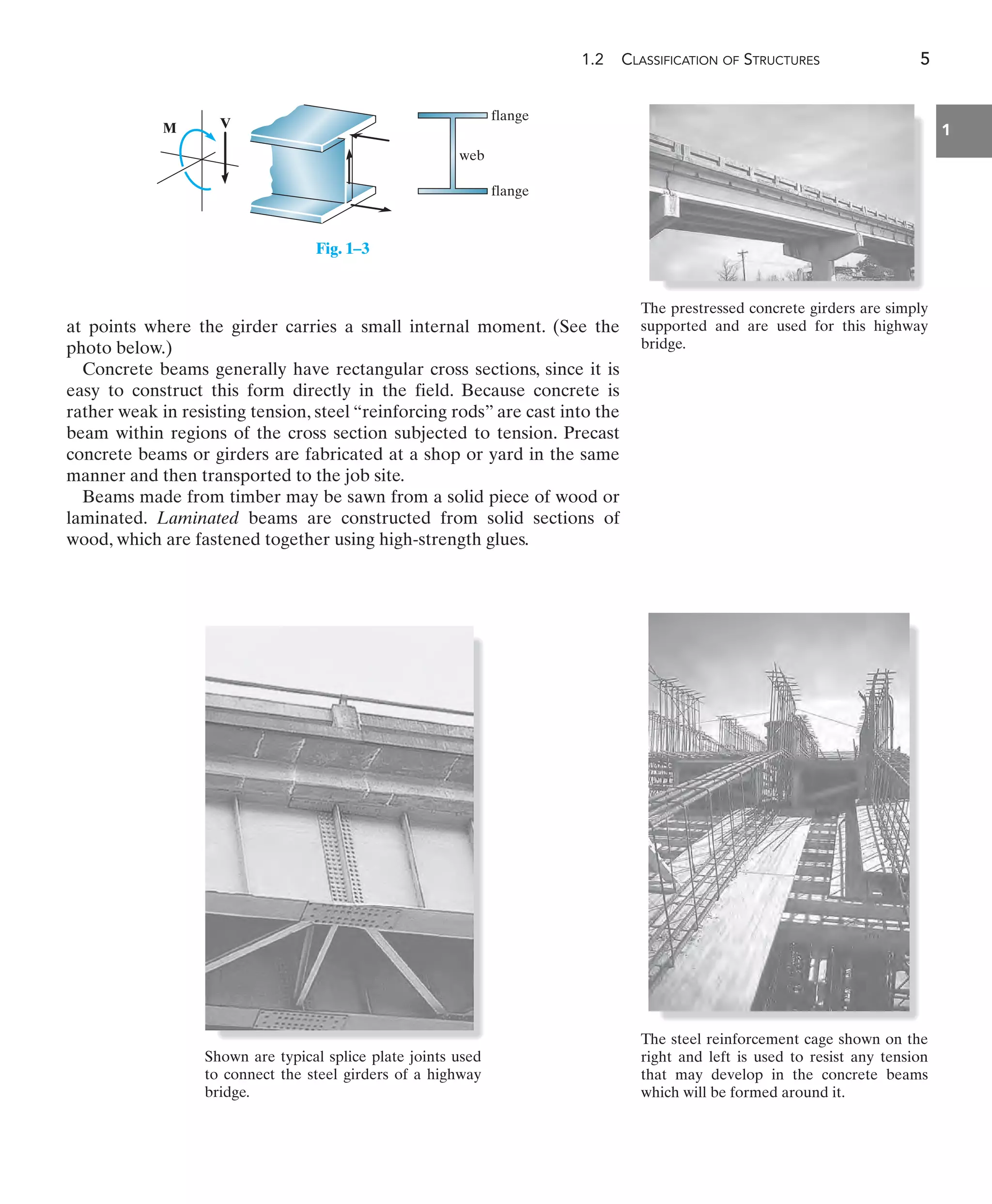
The building roof shown in the photo has a weight of and is
supported on 8-m long simply supported beams that are spaced 1 m
apart. Each beam, shown in Fig. 4–2b transmits its loading to two
girders, located at the front and back of the building. Determine the
internal shear and moment in the front girder at point C, Fig. 4–2a.
Neglect the weight of the members.
1.8 kNm2
Free-Body Diagram. The free-body diagram of the girder is shown
in Fig. 4–2a. Notice that each column reaction is
The free-body diagram of the left girder segment is shown in Fig. 4–2c.
Here the internal loadings are assumed to act in their positive directions.
[1213.6 kN2 + 1117.2 kN2]2 = 43.2 kN
Ans.
Ans.
MC = 30.2 kN # m
- 43.211.22 = 0
MC + 7.210.42 + 7.211.42 + 3.612.42
d+©MC = 0;
VC = 25.2 kN
43.2 - 3.6 - 217.22 - VC = 0
+ c ©Fy = 0;
SOLUTION
Support Reactions. The roof loading is transmitted to each beam
as a one-way slab . The tributary loading
on each interior beam is therefore
(The two edge beams support .) From Fig. 4–2b, the reaction
of each interior beam on the girder is 11.8 kNm218 m22 = 7.2 kN.
0.9 kNm
1.8 kNm.
11.8 kNm2
211 m2 =
1L2L1 = 8 m1 m = 8 7 22

4.1 INTERNAL LOADINGS AT A SPECIFIED POINT 137
4
EXAMPLE 4.2
Determine the internal shear and moment acting at a section passing
through point C in the beam shown in Fig. 4–3a.
SOLUTION
Support Reactions. Replacing the distributed load by its resultant
force and computing the reactions yields the results shown in Fig. 4–3b.
Free-Body Diagram. Segment AC will be considered since it yields
the simplest solution, Fig. 4–3c. The distributed load intensity at C is
computed by proportion, that is,
Ans.
Ans.
This problem illustrates the importance of keeping the distributed
loading on the beam until after the beam is sectioned. If the beam in
Fig. 4–3b were sectioned at C, the effect of the distributed load on
segment AC would not be recognized, and the result and
would be wrong.
MC = 54 k # ft
VC = 9 k
-9162 + 3122 + MC = 0 MC = 48 k # ft
d+©MC = 0;
VC = 6 k
9 - 3 - VC = 0
+ c©Fy = 0;
wC = 16 ft18 ft213 kft2 = 1 kft
A
6 ft
18 ft
C
(a)
3 k/ft
B
27 k
12 ft
(b)
6 ft
9 k 18 k
Fig. 4–3
1 k/ft
NC
MC
9 k
6 ft
2 ft
3 k
(c)
VC

4
EXAMPLE 4.3
The 9-k force in Fig. 4–4a is supported by the floor panel DE, which in
turn is simply supported at its ends by floor beams. These beams
transmit their loads to the simply supported girder AB. Determine the
internal shear and moment acting at point C in the girder.
12 ft 6 ft
4 ft
2 ft
9 k
3 k
5.25 k
24 ft
3.75 k
(b)
3 k
6 k
6 k
C
MC
VC
NC
A
12 ft 3 ft
3.75 k
6 k
(c)
Ans.
Ans.
-3.751152 + 6132 + MC = 0 MC = 38.25 k # ft
d+©MC = 0;
VC = -2.25 k
3.75 - 6 - VC = 0
+ c©Fy = 0;
SOLUTION
Support Reactions. Equilibrium of the floor panel, floor beams, and
girder is shown in Fig. 4–4b. It is advisable to check these results.
Free-Body Diagram. The free-body diagram of segment AC of the
girder will be used since it leads to the simplest solution, Fig. 4–4c.
Note that there are no loads on the floor beams supported by AC.
(a)
6 ft 6 ft
6 ft
4 ft
2 ft
9 k
A
B
C
D E
15 ft
24 ft
Fig. 4–4

4.2 SHEAR AND MOMENT FUNCTIONS 139
4
4.2 Shear and Moment Functions
The design of a beam requires a detailed knowledge of the variations of
the internal shear force V and moment M acting at each point along the
axis of the beam. The internal normal force is generally not considered
for two reasons: (1) in most cases the loads applied to a beam act
perpendicular to the beam’s axis and hence produce only an internal
shear force and bending moment, and (2) for design purposes the beam’s
resistance to shear, and particularly to bending, is more important than
its ability to resist normal force. An important exception to this occurs,
however, when beams are subjected to compressive axial forces, since
the buckling or instability that may occur has to be investigated.
The variations of V and M as a function of the position x of an arbitrary
point along the beam’s axis can be obtained by using the method of
sections discussed in Sec. 4–1. Here, however, it is necessay to locate the
imaginary section or cut at an arbitrary distance x from one end of the
beam rather than at a specific point.
In general,the internal shear and moment functions will be discontinuous,
or their slope will be discontinuous, at points where the type or magnitude
of the distributed load changes or where concentrated forces or couple
moments are applied. Because of this, shear and moment functions
must be determined for each region of the beam located between any
two discontinuities of loading. For example, coordinates and
will have to be used to describe the variation of V and M throughout
the length of the beam in Fig. 4–5a. These coordinates will be valid only
within regions from A to B for from B to C for and from C to D
for Although each of these coordinates has the same origin, as noted
here, this does not have to be the case. Indeed, it may be easier to
develop the shear and moment functions using coordinates
having origins at A, B, and D as shown in Fig. 4–5b. Here and are
positive to the right and is positive to the left.
x3
x2
x1
x3
x2,
x1,
x3.
x2,
x1,
x3
x2,
x1,
Additional reinforcement, provided by ver-
tical plates called stiffeners, is used over the
pin and rocker supports of these bridge
girders. Here the reactions will cause large
internal shear in the girders and the stiff-
eners will prevent localized buckling of the
girder flanges or web. Also, note the tipping
of the rocker support caused by the thermal
expansion of the bridge deck.
A
B C
D
P
w
x1
x2
x3
(a)
A
B C
D
P
w
x1 x2 x3
(b)
Fig. 4–5

4
The following procedure provides a method for determining the
variation of shear and moment in a beam as a function of position x.
Support Reactions
• Determine the support reactions on the beam and resolve all the
external forces into components acting perpendicular and parallel
to the beam’s axis.
Shear and Moment Functions
• Specify separate coordinates x and associated origins,extending into
regions of the beam between concentrated forces and/or couple
moments, or where there is a discontinuity of distributed loading.
• Section the beam perpendicular to its axis at each distance x, and
from the free-body diagram of one of the segments determine the
unknowns V and M at the cut section as functions of x. On the free-
body diagram, V and M should be shown acting in their positive
directions, in accordance with the sign convention given in Fig. 4–1.
• V is obtained from and M is obtained by summing
moments about the point S located at the cut section,
• The results can be checked by noting that and
where w is positive when it acts upward, away from
the beam.These relationships are developed in Sec. 4–3.
dVdx = w,
dMdx = V
©MS = 0.
©Fy = 0
The joists, beams, and girders used to support this floor can be
designed once the internal shear and moment are known
throughout their lengths.

4
EXAMPLE 4.4
Determine the shear and moment in the beam shown in Fig. 4–6a as a
function of x.
2 k/ft
x
30 ft
(a)
Fig. 4–6
20 ft
(b)
30 k
600 k ft
30 k
x
(c)
600 k ft
30 k
x
—
3
M
V
1 x
__ (__) x
2 15
x
w __ k/ft
15
SOLUTION
Support Reactions. For the purpose of computing the support
reactions, the distributed load is replaced by its resultant force of 30 k,
Fig. 4–6b. It is important to remember, however, that this resultant is
not the actual load on the beam.
Shear and Moment Functions. A free-body diagram of the beam
segment of length x is shown in Fig. 4–6c. Note that the intensity of
the triangular load at the section is found by proportion; that is,
or With the load intensity known, the resultant
of the distributed loading is found in the usual manner as shown in the
figure.Thus,
Ans.
Ans.
Note that and which serves as a
check of the results.
dVdx = -x15 = w,
dMdx = V
M = -600 + 30x - 0.0111x3
600 - 30x + c
1
2
a
x
15
bx d
x
3
+ M = 0
d+©MS = 0;
V = 30 - 0.0333x2
30 -
1
2
a
x
15
bx - V = 0
+ c©Fy = 0;
w = x15.
wx = 230

EXAMPLE 4.5
4
14 ft
48 k 60 k
100 kft
6 ft
108 k
1588 kft
(b)
48 k
6 ft
108 k
1588 kft
M
V
x2 6
x2
(d)
60 k
x1 x3 x4
x2
12 ft
20 ft
4 k/ft
100 k· ft
(a)
4x1
1588 k⭈ft
108 k M
V
x1
x1
—
2
(c)
Fig. 4–7
SOLUTION
Support Reactions. The reactions at the fixed support are
and Fig. 4–7b.
Shear and Moment Functions. Since there is a discontinuity of
distributed load at two regions of x must be considered in
order to describe the shear and moment functions for the entire
beam. Here is appropriate for the left 12 ft and can be used for
the remaining segment.
Notice that V and M are shown in the positive
directions, Fig. 4–7c.
Ans.
Ans.
Fig. 4–7d.
Ans.
Ans.
These results can be partially checked by noting that when
then and Also, note that
and dVdx = w.
dMdx = V
M = -100 k # ft.
V = 60 k
x2 = 20 ft,
M = 60x2 - 1300
1588 - 108x2 + 481x2 - 62 + M = 0
d+©MS = 0;
V = 60
108 - 48 - V = 0,
+ c©Fy = 0;
12 ft … x2 … 20 ft,
M = -1588 + 108x1 - 2x1
2
1588 - 108x1 + 4x1 a
x1
2
b + M = 0
d+©MS = 0;
V = 108 - 4x1
108 - 4x1 - V = 0,
+ c©Fy = 0;
0 … x1 … 12 ft.
x2
x1
x = 12 ft,
M = 1588 k # ft,
V = 108 k
function of x.

4
Fig. 4–8
EXAMPLE 4.6
function of x.
10 kN/m
30 kN/m
9 m
x
(a)
75 kN
20 kN/m
9 m
(b)
90 kN 90 kN
6 m
4.5 m
105 kN
10 kN/m
x
20(__) kN/m
9
10 kN/m
75 kN
10x
x
–
2
x
–
2
x
–
3
M
V
(c)
1 x
__ (20)(__) x
2 9
SOLUTION
Support Reactions. To determine the support reactions, the
distributed load is divided into a triangular and rectangular loading,
and these loadings are then replaced by their resultant forces. These
reactions have been computed and are shown on the beam’s free-
body diagram, Fig. 4–8b.
Shear and Moment Functions. A free-body diagram of the cut
section is shown in Fig. 4–8c. As above, the trapezoidal loading is
replaced by rectangular and triangular distributions. Note that the
intensity of the triangular load at the cut is found by proportion. The
resultant force of each distributed loading and its location are
indicated.Applying the equilibrium equations, we have
Ans.
Ans.
M = 75x - 5x2
- 0.370x3
-75x + 110x2a
x
2
b + c
1
2
1202a
x
9
bxd
x
3
+ M = 0
d+©MS = 0;
V = 75 - 10x - 1.11x2
75 - 10x - c
1
2
1202a
x
9
bx d - V = 0
+ c©Fy = 0;

4
F4–1. Determine the internal normal force, shear force,
and bending moment acting at point C in the beam.
A
C
B
2 m 1 m 2 m
1 m
10 kN
20 kN⭈m
F4–1
A B
8 kN/m
4 kN/m
1.5 m 1.5 m
C
F4–2
A B
C
6 kN/m
1.5 m 3 m
1.5 m
F4–3
A
B
300 lb/ft
3 ft
1.5 ft
1.5 ft
C
F4–4
1.5 m
3 m
3 m
45⬚
A B
C
5 kN/m
F4–5
800 lb
600 lb
A
C
B
150 lb/ft
3 ft 3 ft
3 ft 6 ft
F4–6

4
F4–7. Determine the internal shear and moment in the
beam as a function of x.
beam as a function of x throughout the beam.
B
3 m
6 kN
18 kN/m
A
x
F4–7
A B
12 kN/m
6 m
x
F4–8
A B
8 kN/m
4 m 4 m
x
F4–9
5 kN/m
A B
2 m 2 m
x
15 kN ·m
20 kN ·m
F4–10
5 kN/m
A
2 m 2 m
15 kN
x
F4–11
A B
2 k/ft
12 ft 12 ft
x
18 k
F4–12

4
4–2. Determine the internal normal force, shear force, and
bending moment in the beam at points C and D. Assume
the support at B is a roller. Point D is located just to the
right of the 10-k load.
*4–4. Determine the internal normal force, shear force,
and bending moment at point D.Take w 150 N兾m.
4–5. The beam AB will fail if the maximum internal
moment at D reaches or the normal force in
member BC becomes 1500 N. Determine the largest load w
it can support.
800 N # m
=
the support at A is a pin and B is a roller.
4–3. The boom DF of the jib crane and the column DE
have a uniform weight of 50 lb兾ft. If the hoist and load weigh
300 lb, determine the internal normal force, shear force, and
bending moment in the crane at points A, B, and C.
PROBLEMS
6 kN
20 kN·m
B
A C D
1 m 1 m 2 m 2 m
Prob. 4–1
10 ft 10 ft 10 ft
A
C D B
10 k
25 k·ft 25 k·ft
Prob. 4–2
5 ft
7 ft
C
D
F
E
B A
300 lb
2 ft 8 ft 3 ft
Prob. 4–3
4 m
A
D
B
C
4 m
4 m
3 m
w
Probs. 4–4/4–5

4
the support at A is a roller and B is a pin.
bending moment in the beam at point C. The support at A is
a roller and B is pinned.
bending moment at point C. Assume the reactions at the
supports A and B are vertical.
4–10. Determine the internal normal force, shear force,
and bending moment at point C. Assume the reactions at
the supports A and B are vertical.
A B
1.5 m
1.5 m
4 kN/m
C D
1.5 m
1.5 m
Prob. 4–6
D
A B
0.5 kN/m
1.5 kN/m
3 m
6 m
Prob. 4–8
3 m
C
A B
0.5 kN/m
1.5 kN/m
6 m
Prob. 4–7
5 kN
A C B
3 kN/m
1 m 2 m 2 m
Prob. 4–9
6 ft
A B
300 lb/ft
4.5 ft
400 lb/ft
4.5 ft
E
D
14 ft
Prob. 4–11
8 ft
C
A B
300 lb/ft
400 lb/ft
12 ft 9 ft
Prob. 4–10
*4–8. Determine the internal normal force, shear force,
and bending moment at point D. Assume the reactions at
bending moment at points D and E.Assume the reactions at

4
B
A
x
a b
L
P
Prob. 4–12
2 m 1 m
1 m
A
x
B
4 kN
6 kN
Prob. 4–13
*4–12. Determine the shear and moment throughout the
4–15. Determine the shear and moment throughout the
4–13. Determine the shear and moment in the floor girder
as a function of x.Assume the support at A is a pin and B is
a roller.
*4–16. Determine the shear and moment throughout the
B
A
x
a b
M0
L
Prob. 4–14
B
A
4 m
2 m
2 m
x
12 kN⭈m
7 kN
Prob. 4–15
A B
8 kN/m
3 m
3 m
x
Prob. 4–16
1 m 1 m 1 m
8 kN
8 kN
4 kN
A
x
Prob. 4–17

4
beam as functions of x.
4–21. Determine the shear and moment in the beam as a
function of x.
beam as functions of x.
tapered beam as a function of x.
*4–20. Determine the shear and moment in the beam as
functions of x.
6 ft 4 ft
2 k/ft
8 k
x
10 k
40 k⭈ft
Prob. 4–18
A B
x
4 ft 4 ft
150 lb/ft
6 ft
250 lb
250 lb
Prob. 4–19
x
B
A
w0
L
__
2
L
__
2
Prob. 4–20
A B
200 lb/ft
10 ft
800 lb
1200 lb⭈ft
x
Prob. 4–21
8 kN/m
x
9 m
A
B
Prob. 4–22

4
for a Beam
If the variations of V and M as functions of x obtained in Sec. 4–2 are
plotted, the graphs are termed the shear diagram and moment diagram,
respectively. In cases where a beam is subjected to several concentrated
forces, couples, and distributed loads, plotting V and M versus x can
become quite tedious since several functions must be plotted. In this
section a simpler method for constructing these diagrams is discussed—a
method based on differential relations that exist between the load, shear,
and moment.
To derive these relations, consider the beam AD in Fig. 4–9a, which is
subjected to an arbitrary distributed loading and a series of
concentrated forces and couples. In the following discussion, the
distributed load will be considered positive when the loading acts upward
as shown. We will consider the free-body diagram for a small segment of
the beam having a length Fig.4–9b.Since this segment has been chosen
at a point x along the beam that is not subjected to a concentrated force
or couple, any results obtained will not apply at points of concentrated
loading.The internal shear force and bending moment shown on the free-
body diagram are assumed to act in the positive direction according to the
established sign convention, Fig. 4–1. Note that both the shear force and
moment acting on the right face must be increased by a small, finite
amount in order to keep the segment in equilibrium. The distributed
loading has been replaced by a concentrated force that acts at a
fractional distance from the right end, where (For
example, if w(x) is uniform or constant, then will act at so
.) Applying the equations of equilibrium, we have
¢M = V¢x + w1x2 P1¢x22
-V¢x - M - w1x2 ¢x P1¢x2 + 1M + ¢M2 = 0
d+©MO = 0;
¢V = w1x2 ¢x
V + w1x2 ¢x - 1V + ¢V2 = 0
+ c©Fy = 0;
P = 1
2
1
2 ¢x,
w1x2¢x
0 6 P 6 1.
P1¢x2
w1x2¢x
¢x,
w = w1x2
M1
B C
M2
x x
F1
F2 F3
w w(x)
w
x
D
A
(a)
x
V V
(b)
w(x)x
w(x)
M
V
M M
O
P (x)
Fig. 4–9
The many concentrated loadings acting
on this reinforced concrete beam create a
variation of the internal loading in the
beam. For this reason, the shear and moment
diagrams must be drawn in order to properly
design the beam.

4.3 SHEAR AND MOMENT DIAGRAMS FOR A BEAM 151
4
Dividing by and taking the limit as these equations become
(4–1)
(4–2)
As noted, Eq. 4–1 states that the slope of the shear diagram at a point
(dV兾dx) is equal to the intensity of the distributed load w(x) at the point.
Likewise, Eq. 4–2 states that the slope of the moment diagram (dM兾dx) is
equal to the intensity of the shear at the point.
Equations 4–1 and 4–2 can be “integrated” from one point to another
between concentrated forces or couples (such as from B to C in Fig. 4–9a),
in which case
(4–3)
and
(4–4)
As noted, Eq. 4–3 states that the change in the shear between any two
points on a beam equals the area under the distributed loading diagram
between the points. Likewise, Eq. 4–4 states that the change in the moment
between the two points equals the area under the shear diagram between
the points. If the areas under the load and shear diagrams are easy to
compute,Eqs.4–3 and 4–4 provide a method for determining the numerical
values of the shear and moment at various points along a beam.
Change in
Moment
f = e
Area under
Shear Diagram
¢M =
L
V1x2 dx
Change in
Shear
f = c
Area under
Distributed Loading
Diagram
¢V =
L
w1x2 dx
Slope of
Moment Diagram
f = 5Shear
dM
dx
= V
Slope of
Shear Diagram
f = e
Intensity of
Distributed Load
dV
dx
= w1x2
¢x : 0,
¢x

4
From the derivation it should be noted that Eqs. 4–1 and 4–3 cannot be
used at points where a concentrated force acts, since these equations do
not account for the sudden change in shear at these points. Similarly,
because of a discontinuity of moment, Eqs. 4–2 and 4–4 cannot be used at
points where a couple moment is applied. In order to account for these
two cases, we must consider the free-body diagrams of differential
elements of the beam in Fig. 4–9a which are located at concentrated
force and couple moments. Examples of these elements are shown in
Figs. 4–10a and 4–10b, respectively. From Fig. 4–10a it is seen that force
equilibrium requires the change in shear to be
(4–5)
Thus,when F acts downward on the beam, is negative so that the shear
diagram shows a “jump” downward. Likewise, if F acts upward, the jump
is upward. From Fig. 4–10b, letting moment equilibrium
requires the change in moment to be
(4–6)
In this case, if an external couple moment is applied clockwise,
is positive, so that the moment diagram jumps upward, and when M acts
counterclockwise, the jump must be downward.
1¢M2
¢M
M¿
¢M = M¿
d+©MO = 0;
¢x : 0,
1¢V2
¢V
¢V = -F
+ c ©Fy = 0;
F
M
V V V
M M
(a)
x
M¿
M
V x
V V
(b)
M M
O
Fig. 4–10

4
The following procedure provides a method for constructing the shear
and moment diagrams for a beam using Eqs. 4–1 through 4–6.
Support Reactions
• Determine the support reactions and resolve the forces acting on
the beam into components which are perpendicular and parallel
to the beam’s axis.
Shear Diagram
• Establish the V and x axes and plot the values of the shear at the
two ends of the beam.
• Since the slope of the shear diagram at any point is
equal to the intensity of the distributed loading at the point. (Note
that w is positive when it acts upward.)
• If a numerical value of the shear is to be determined at the point,
one can find this value either by using the method of sections as
discussed in Sec. 4–1 or by using Eq. 4–3, which states that the
change in the shear force is equal to the area under the distributed
loading diagram.
• Since w(x) is integrated to obtain V, if w(x) is a curve of degree n,
then V(x) will be a curve of degree For example, if w(x) is
uniform, V(x) will be linear.
Moment Diagram
• Establish the M and x axes and plot the values of the moment at
the ends of the beam.
• Since the slope of the moment diagram at any point
is equal to the intensity of the shear at the point.
• At the point where the shear is zero, and therefore
this may be a point of maximum or minimum moment.
• If the numerical value of the moment is to be determined at a
point, one can find this value either by using the method of
sections as discussed in Sec. 4–1 or by using Eq. 4–4, which states
that the change in the moment is equal to the area under the shear
diagram.
• Since V(x) is integrated to obtain M, if V(x) is a curve of degree n,
then M(x) will be a curve of degree For example, if V(x) is
linear, M(x) will be parabolic.
n + 1.
dMdx = 0,
dMdx = V,
n + 1.
dVdx = w,

4
The two horizontal members of the power line support frame are
subjected to the cable loadings shown in Fig. 4–11a. Draw the shear
and moment diagrams for each member.
SOLUTION
Support Reactions. Each pole exerts a force of 6 kN on each
member as shown on the free-body diagram.
Shear Diagram. The end points and
are plotted first, Fig. 4–11b.As indicated, the shear between
each concentrated force is constant since The shear
just to the right of point B (or C and D) can be determined by the
method of sections,Fig.4–11d.The shear diagram can also be established
by “following the load” on the free-body diagram. Beginning at A the
4 kN load acts downward so No load acts between A
and B so the shear is constant.At B the 6 kN force acts upward, so the
shear jumps up 6 kN, from to , etc.
Moment Diagram. The moment at the end points and
is plotted first, Fig. 4–11c. The slope of the moment
diagram within each 1.5-m-long region is constant because V is
constant. Specific values of the moment, such as at C, can be deter-
mined by the method of sections, Fig. 4–11d, or by finding the change
in moment by the area under the shear diagram. For example, since
at A, then at C,
.
= -3 kN # m
+ 211.52
0 + 1-4211.52
=
MC = MA + ¢MAC
MA = 0
x = 6 m, M = 0
x = 0, M = 0
+2 kN
-4 kN
VA = -4 kN.
w = dVdx = 0.
V = 4 kN
x = 6 m,
x = 0, V = -4 kN
EXAMPLE 4.7
6 kN
6 kN
4 kN 4 kN
4 kN
1.5 m 1.5 m 1.5 m 1.5 m
(c)
(b)
(a)
1.5
6 6
3
3
2
4
4.5 6
x (m)
M (kNm)
8
2
4
3
1.5 4.5 6
x (m)
V (kN)
A B C D E
V negative constant
M slope negative constant
V positive constant
M slope positive constant
w 0
V slope 0
w 0
V slope 0
6 kN
4 kN
1.5 m 1.5 m
(d)
VC
MC
Fig. 4–11

4
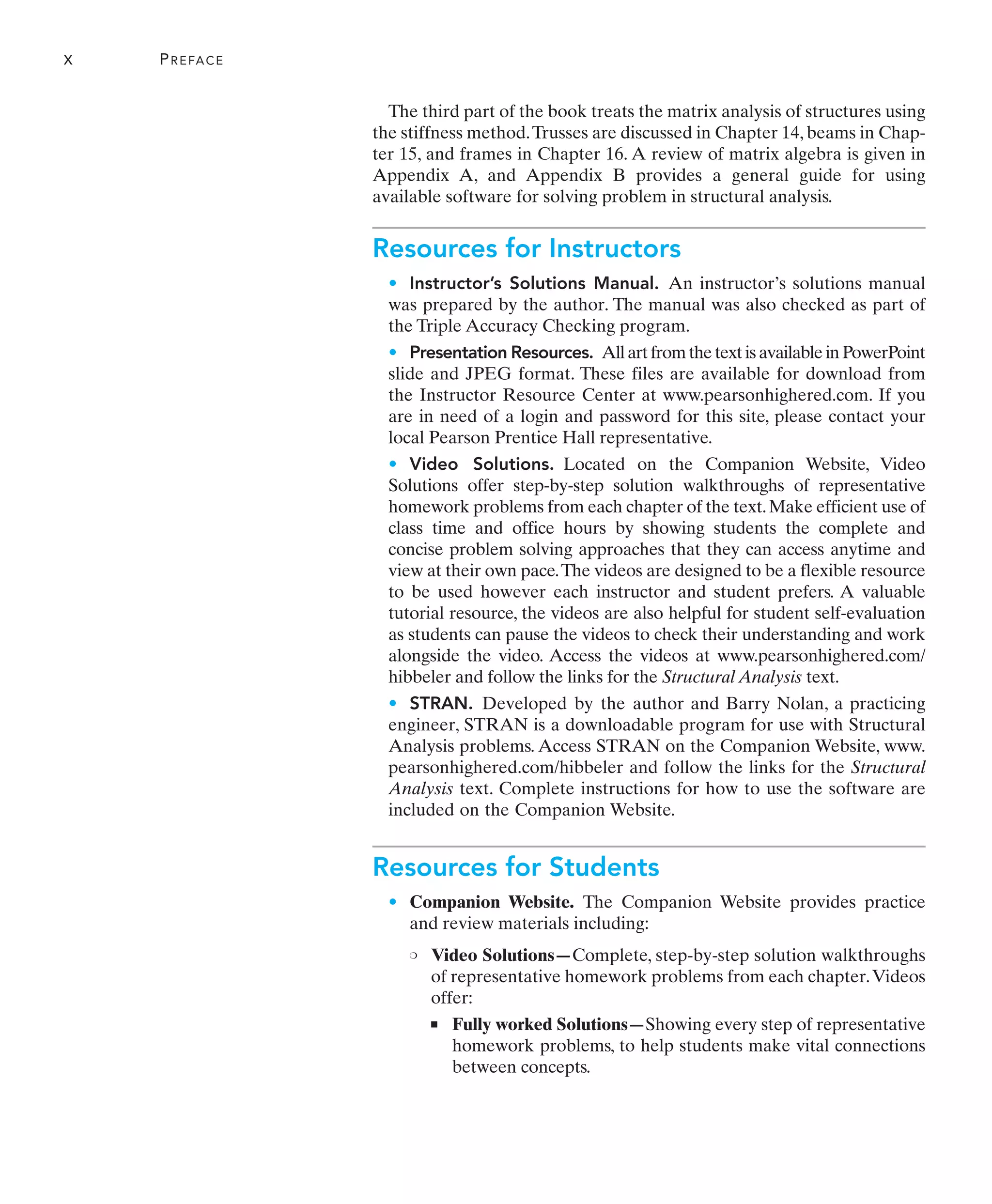
EXAMPLE 4.8
Draw the shear and moment diagrams for the beam in Fig. 4–12a.
9 m
20 kN/m
(a)
V (kN)
30
⫺60
x (m)
(c)
5.20 m
20 kN/m
(b)
30 kN 60 kN
104
M (kN⭈m)
x (m)
(d)
V positive decreasing
M slope positive decreasing
w negative increasing
V slope negative increasing
V negative increasing
M slope negative increasing
Fig. 4–12
SOLUTION
Support Reactions. The reactions have been calculated and are
shown on the free-body diagram of the beam, Fig. 4–12b.
Shear Diagram. The end points and
are first plotted. Note that the shear diagram starts
with zero slope since at and ends with a slope of
The point of zero shear can be found by using the method of
sections from a beam segment of length x,Fig.4–12e.We require
so that
Moment Diagram. For the value of shear is
positive but decreasing and so the slope of the moment diagram is also
positive and decreasing At
Likewise for the shear and so the slope of the
moment diagram are negative increasing as indicated.
The maximum value of moment is at since
at this point, Fig. 4–12d. From the free-body diagram in
Fig. 4–12e we have
M = 104 kN # m
-3015.202 +
1
2
c20a
5.20
9
b d15.202a
5.20
3
b + M = 0
d+©MS = 0;
V = 0
dMdx =
x = 5.20 m
5.20 m 6 x 6 9 m,
dMdx = 0.
x = 5.20 m,
1dMdx = V2.
0 6 x 6 5.20 m
30 -
1
2
c20a
x
9
b dx = 0 x = 5.20 m
+ c ©Fy = 0;
V = 0,
w = -20 kN/m.
x = 0,
w = 0
V = -60 kN
x = 9 m,
V = +30 kN
x = 0,
(e)
30 kN
[20 ( )]x
1
—
2
x
—
9
x
—
9
20 ( )
V
M
x
x
—
3

4
Draw the shear and moment diagrams for the beam shown in Fig.4–13a.
SOLUTION
Support Reactions. The reactions are calculated and indicated on
the free-body diagram.
Shear Diagram. The values of the shear at the end points A
and B are plotted.At C the shear is
discontinuous since there is a concentrated force of 600 lb there. The
value of the shear just to the right of C can be found by sectioning
the beam at this point. This yields the free-body diagram shown in
equilibrium in Fig. 4–13e. This point is plotted on the
shear diagram. Notice that no jump or discontinuity in shear occurs
at D, the point where the couple moment is applied,
Fig. 4–13b.
Moment Diagram. The moment at each end of the beam is zero,
Fig. 4–13d. The value of the moment at C can be determined by the
method of sections, Fig. 4–13e, or by finding the area under the shear
diagram between A and C. Since
Also, since the moment at D is
A jump occurs at point D due to the couple moment of
The method of sections, Fig. 4–13f, gives a value of just to
the right of D.
+2500 lb # ft
4000 lb # ft.
MD = -1500 lb # ft
MD = MC + ¢MCD = 1000 lb # ft + 1-500 lb215 ft2
MC = 1000 lb # ft,
MC = 1000 lb # ft
MC = MA + ¢MAC = 0 + 1100 lb)(10 ft)
MA = 0,
4000-lb # ft
1V = -500 lb2
1VB = -500 lb2
1VA = +100 lb2
EXAMPLE 4.9
10 ft 5 ft 5 ft
C D
600 lb
4000 lb⭈ft
(a)
B
A
V negative constant
M slope negative constant
V (lb)
100 x (ft)
⫺500
(c)
10 ft 5 ft
600 lb
4000 lb⭈ft
100 lb 500 lb
(b)
5 ft
M (lb⭈ft)
2500
⫺1500
1000
(d)
x (ft)
w =0
slope =0
V
10 ft
600 lb
1000 lb⭈ft
100 lb
(e)
⫺500 lb
C 10 ft 5 ft
600 lb
100 lb
(f)
2500 lb⭈ft
⫺500 lb
4000 lb⭈ft
D
Fig. 4–13

4
EXAMPLE 4.10
Draw the shear and moment diagrams for each of the beams shown in
Fig. 4–14.
SOLUTION
In each case the support reactions have been calculated and are
shown in the top figures. Following the techniques outlined in the pre-
vious examples, the shear and moment diagrams are shown under
each beam. Carefully notice how they were established, based on the
slope and moment, where and Calculated
values are found using the method of sections or finding the areas
under the load or shear diagrams.
dMdx = V.
dVdx = w
3 m
9 kN 9 kN
6 kN/m
3 m
x (m)
x (m)
V (kN)
M (kN⭈m)
9
3
3 6
–9
18
(a)
4 ft
6 k/ft
15 k
8 k
47 k
4 ft
(c)
4
⫺80
⫺20
8
x (ft)
M (k⭈ft)
20 k⭈ft
⫺15
8
8
32
4
x (ft)
V (k)
V positive decreasing
M slope positive decreasing
w negative constant
V slope negative constant
3 m
30 kN
8 kN/m
1.5 m
42 kN⭈m
15 kN⭈m
15
2.64
⫺42
⫺30
⫺6
1.5
12
1.5 4.5
x (m)
x (m)
V (kN)
M (kN⭈m)
(b)
Fig. 4–14

4
Fig. 4–15
The beam shown in the photo is used to support a portion of the
overhang for the entranceway of the building.The idealized model for
the beam with the load acting on it is shown in Fig. 4–15a.Assume B is
a roller and C is pinned. Draw the shear and moment diagrams for the
beam.
SOLUTION
Support Reactions. The reactions are calculated in the usual
manner.The results are shown in Fig. 4–15b.
Shear Diagram. The shear at the ends of the beam is plotted first,
i.e., and Fig.4–15c.To find the shear to the left
of B use the method of sections for segment AB, or calculate the area
under the distributed loading diagram, i.e.,
The support reaction causes the shear to jump up
The point of zero shear can be determined
from the slope or by proportional triangles,
Notice how the V diagram follows the
negative slope,defined by the constant negative distributed loading.
Moment Diagram. The moment at the end points is plotted first,
Fig. 4–15d. The values of and 0.239 on the
moment diagram can be calculated by the method of sections, or by
finding the areas under the shear diagram. For example,
Likewise,
show that the maximum positive moment is Notice
how the M diagram is formed, by following the slope, defined by the
V diagram.
0.239 kN # m.
MB = -2.81 kN # m.
MB - 0 = 1
21-7.50210.752 = -2.81,
¢M =
-2.81
MA = MC = 0,
x = 0.781 m.
2.1911 - x2,
7.81x =
-10 kNm,
-7.50 + 15.31 = 7.81 kN.
VB- = -7.50 kN.
¢V = VB - 0 = -1010.752,
VC = -2.19 kN,
VA = 0
EXAMPLE 4.11
0.75 m
10 kN/m
1 m
A B C
(a)
0.75 m
10 kN/m
1 m
A B C
2.19 kN
15.31 kN
(b)
x (m)
V (kN)
⫺7.50
⫺2.19
7.81
0.781 m
(c)
⫺2.81
0.239
x (m)
M (kN⭈m)
(d)

4
EXAMPLE 4.12
Draw the shear and moment diagrams for the compound beam shown
in Fig. 4–16a.Assume the supports at A and C are rollers and B and E
are pin connections.
SOLUTION
Support Reactions. Once the beam segments are disconnected
from the pin at B, the support reactions can be calculated as shown in
Fig. 4–16b.
Shear Diagram. As usual, we start by plotting the end shear at A
and E, Fig. 4–16c. The shape of the V diagram is formed by following
its slope, defined by the loading. Try to establish the values of shear
using the appropriate areas under the load diagram (w curve) to find
the change in shear.The zero value for shear at can either be
found by proportional triangles, or by using statics, as was done in
Fig. 4–12e of Example 4–8.
Moment Diagram. The end moments and
are plotted first, Fig. 4–16d. Study the diagram and note how the
various curves are established using Verify the numerical
values for the peaks using statics or by calculating the appropriate
areas under the shear diagram to find the change in moment.
dMdx = V.
ME = 0
MA = 60 k # ft
x = 2 ft
A B C D E
10 ft 6 ft 4 ft 6 ft
5 k
2 k/ft
3 k/ft
60 k · ft
(a)
6 ft
20 k 5 k 3 k/ft
60 k⭈ft
4 k
16 k
16 k
0
45 k 6 k
0
(b)
V (k)
4 2 10 16 20
⫺16
⫺21
24
6
32
x (ft)
(c)
M (k⭈ft)
64
60
2
10 16 20
⫺96
⫺180
32
x (ft)
(d)
Fig. 4–16

4
F4–13. Draw the shear and moment diagrams for the
beam. Indicate values at the supports and at the points
where a change in load occurs.
B
2 m
2 m
3 kN
A
8 kN
F4–13
B
A
4 m 2 m
2 m
6 kN
6 kN ·m
8 kN
F4–14
2 k/ft
A
10 ft
30 k·ft
F4–15
12 ft 12 ft
6 k/ft
A B
18 k
x
F4–16
A B
2 kN/m
2 kN/m
4.5 m
4.5 m
F4–17
A B
4 kN/m
1.5 m 2 m 1.5 m
F4–18
A B
6 kN/m
2 m 2 m 2 m
6 kN/m
F4–19
A B
2 k/ft
6 ft 6 ft
F4–20

4–23. Draw the shear and moment diagrams for the beam. 4–26. Draw the shear and moment diagrams for the beam.
PROBLEMS
6 ft
A
C D
E
B
6 ft
2 ft
4 ft 4 ft
500 lb
200 lb 300 lb
Prob. 4–23
4 ft
4 ft
4 ft
4 ft
4 ft
2 k 2 k 2 k
4 ft
4 ft
4 ft
4 ft
4 ft
A
2 k
Prob. 4–24
*4–24. Draw the shear and moment diagrams for the beam.
4–25. Draw the shear and moment diagrams for the beam.
B
D
A
2 m
1 m 2 m
1 m
0.4 m
6 kN
3
5
4
C
0.6 m
20 kN · m
Prob. 4–25
10 k 8 k
A C B
0.8 k/ft
6 ft 6 ft
12 ft 12 ft
Prob. 4–26
x
15 ft
600 lb⭈ft
A B
400 lb/ft
Prob. 4–27
L/3 L/3 L/3
M0
M0
Prob. 4–28
C
A
B
2 m
3 m
1.5 kN/m
Prob. 4–29
*4–28. Draw the shear and moment diagrams for the
beam (a) in terms of the parameters shown; (b) set
L = 8 m.
M0 = 500 N # m,

4
4–30. Draw the shear and bending-moment diagrams for
the beam.
C
A
B
20 ft 10 ft
50 lb/ft
200 lb⭈ft
Prob. 4–30
C
w
A
B
L
L
––
2
Prob. 4–31
250 lb/ft
150 lb ⭈ ft
150 lb ⭈ ft
A B
20 ft
Prob. 4–32
40 kN/m
20 kN
150 kN⭈m
A
B
8 m 3 m
Prob. 4–33
*4–36. Draw the shear and moment diagrams of the beam.
Assume the support at B is a pin and A is a roller.
*4–32. Draw the shear and moment diagrams for the beam.
x
4 ft 4 ft 4 ft 4 ft
200 lb/ft
C D E F G
A B
Prob. 4–34
A B
200 lb/ft
30 ft
800 lb
1200 lb⭈ft
Prob. 4–35
A B
800 lb · ft
100 lb/ft
16 ft
4 ft
Prob. 4–36
B
8 kN/m
1.5 m 6 m
A
Prob. 4–37
Assume the support at B is a pin.

4.4 SHEAR AND MOMENT DIAGRAMS FOR A FRAME 163
4
for a Frame
Recall that a frame is composed of several connected members that are
either fixed or pin connected at their ends. The design of these
structures often requires drawing the shear and moment diagrams for
each of the members. To analyze any problem, we can use the
procedure for analysis outlined in Sec. 4–3. This requires first
determining the reactions at the frame supports. Then, using the
method of sections, we find the axial force, shear force, and moment
acting at the ends of each member. Provided all loadings are resolved
into components acting parallel and perpendicular to the member’s
axis, the shear and moment diagrams for each member can then be
drawn as described previously.
When drawing the moment diagram, one of two sign conventions is
used in practice. In particular, if the frame is made of reinforced concrete,
designers often draw the moment diagram positive on the tension side of
the frame. In other words, if the moment produces tension on the outer
surface of the frame, the moment diagram is drawn positive on this side.
Since concrete has a low tensile strength, it will then be possible to tell at
a glance on which side of the frame the reinforcement steel must be
placed. In this text, however, we will use the opposite sign convention
and always draw the moment diagram positive on the compression side of
the member. This convention follows that used for beams discussed in
Sec. 4–1.
The following examples illustrate this procedure numerically.
The simply supported girder of this concrete building frame was
designed by first drawing its shear and moment diagrams.

4
Draw the moment diagram for the tapered frame shown in Fig. 4–17a.
Assume the support at A is a roller and B is a pin.
EXAMPLE 4.13
15 ft
5 k
C
5 ft
6 ft
3 k
(a)
A
B
Fig. 4–17
15 ft
5 k
5 ft
6 ft
3 k
3 k
1 k
(b)
6 k
5 ft
3 k
6 k
15 kft
3 k
6 k
A
5 k 1 k
3 k
15 kft
3 k
15 kft
C
6 k
15 kft
3 k
1 k
B
15 ft
1 k
3 k
(c)
15
15
15
6
11
(d)
M (kft)
member CB
member AC
M (kft)
x (ft)
x (ft)
SOLUTION
Support Reactions. The support reactions are shown on the
free-body diagram of the entire frame, Fig. 4–17b. Using these results,
the frame is then sectioned into two members, and the internal reac-
tions at the joint ends of the members are determined, Fig. 4–17c.
Note that the external 5-k load is shown only on the free-body diagram
of the joint at C.
Moment Diagram. In accordance with our positive sign convention,
and using the techniques discussed in Sec. 4–3, the moment diagrams
for the frame members are shown in Fig. 4–17d.

4
EXAMPLE 4.14
Draw the shear and moment diagrams for the frame shown in
Fig. 4–18a. Assume A is a pin, C is a roller, and B is a fixed joint.
Neglect the thickness of the members.
SOLUTION
Notice that the distributed load acts over a length of
The reactions on the entire frame are calculated
and shown on its free-body diagram, Fig. 4–18b. From this diagram the
free-body diagrams of each member are drawn, Fig. 4–18c. The
distributed loading on BC has components along BC and perpendicular
to its axis of
as shown. Using these results, the shear and moment diagrams are
also shown in Fig. 4–18c.
10.1414 kft2 cos 45° = 10.1414 kft2 sin 45° = 0.1 kft
10 ft 22 = 14.14 ft.
10 ft
1
4
.
1
4
f
t
1
.
0
6

5
0
.
3
5
4
k
1
0
.
6
0
.
6
2
5
0.5 k
0.5 k
2 k
2 k
(c)
0.5 k
1.06 k
1.77 k
1.77 k
2 k
0.5 k
1.06 k
0.1 k/ft
0.1 k/ft
5 kft
5 kft
5 kft
5 kft
M
(
k

f
t
)
M
(kft)
V
(
k
)
x
(
f
t
)
0.5
V
(k)
x
(ft)
–5
x
(ft)
x
(
f
t
)
Fig. 4–18
10 ft
0.1414 k/ft
10 ft
10 ft
A
B
C
(a)
20 ft
5 ft
(0.1414 k/ft)(14.14 ft) 2 k 0.5 k
0.5 k
2 k
(b)

4
EXAMPLE 4.15
Draw the shear and moment diagrams for the frame shown in Fig.4–19a.
Assume A is a pin, C is a roller, and B is a fixed joint.
40 kN/m
B
4 m
4 m
C
3 m
2 m
80 kN
A
(a)
Fig. 4–19
120 kN
2 m
6 m
80 kN
(b)
1.5 m
Cy 82.5 kN
36.87
Ay 2.5 kN
Ax 120 kN
SOLUTION
Support Reactions. The free-body diagram of the entire frame is
shown in Fig. 4–19b. Here the distributed load, which represents wind
loading, has been replaced by its resultant, and the reactions have been
computed. The frame is then sectioned at joint B and the internal
loadings at B are determined, Fig. 4–19c. As a check, equilibrium is
satisfied at joint B, which is also shown in the figure.
Shear and Moment Diagrams. The components of the distributed
load, and
are shown on member AB, Fig. 4–19d. The associated shear and
moment diagrams are drawn for each member as shown in Figs. 4–19d
and 4–19e.
196 kN215 m2 = 19.2 kNm,
172 kN215 m2 = 14.4 kNm

4
96 kN
2 kN
36.87
1.5 kN
72 kN
96 kN
72 kN
36.87
170 kNm
B
2 kN
1.5 kN
A
36.87
170 kNm
2.5 kN
B
170 kNm
1.5 kN 2 kN
B
2.5 kN
170 kNm
80 kN
C
82.5 kN
(c)
14.4 kN/m
70 kN
97.5 kN
A
19.2 kN/m
5 m
B
170 kNm
1.5 kN
2 kN
x (m)
4.86
2
170.1
170
4.86
x (m)
V (kN)
M (kNm)
70
(d)
B
2.5 kN
170 kNm
80 kN
C
82.5 kN
(e)
x (m)
2.5
V (kN)
2
82.5
M (kNm)
170 165
2
x (m)

4
4.5 Moment Diagrams Constructed by
the Method of Superposition
Since beams are used primarily to resist bending stress, it is important
that the moment diagram accompany the solution for their design. In
Sec. 4–3 the moment diagram was constructed by first drawing the shear
diagram. If we use the principle of superposition, however, each of the
loads on the beam can be treated separately and the moment diagram
can then be constructed in a series of parts rather than a single and
sometimes complicated shape. It will be shown later in the text that this
can be particularly advantageous when applying geometric deflection
methods to determine both the deflection of a beam and the reactions
on statically indeterminate beams.
Most loadings on beams in structural analysis will be a combination of
the loadings shown in Fig. 4–20. Construction of the associated moment
diagrams has been discussed in Example 4–8. To understand how to use
P
L
M
PL
x
(a)
Fig. 4–20
M0
L
M
x
(b)
M0
L
L
M
x
(c)
w0
parabolic curve
w0 L2
______
2
L
M
x
(d)
w0
w0 L2
______
6
cubic curve

4.5 MOMENT DIAGRAMS CONSTRUCTED BY THE METHOD OF SUPERPOSITION 169
4
the method of superposition to construct the moment diagram consider
the simply supported beam at the top of Fig. 4–21a. Here the reactions
have been calculated and so the force system on the beam produces a zero
force and moment resultant.The moment diagram for this case is shown at
the top of Fig. 4–21b. Note that this same moment diagram is produced for
the cantilevered beam when it is subjected to the same statically equivalent
system of loads as the simply supported beam. Rather than considering all
the loads on this beam simultaneously when drawing the moment diagram,
we can instead superimpose the results of the loads acting separately on
the three cantilevered beams shown in Fig. 4–21a. Thus, if the moment
diagram for each cantilevered beam is drawn,Fig.4–21b,the superposition
of these diagrams yields the resultant moment diagram for the simply
supported beam.For example,from each of the separate moment diagrams,
the moment at end A is as verified by the
top moment diagram in Fig. 4–21b. In some cases it is often easier to
construct and use a separate series of statically equivalent moment
diagrams for a beam, rather than construct the beam’s more complicated
“resultant” moment diagram.
MA = -200 - 300 + 500 = 0,
4 k/ft
A
300 kft
B
10 ft 10 ft
15 k 25 k
4 k/ft
10 ft
40 k
200 kft
ⴝ
ⴙ
10 ft
300 kft
300 kft
ⴙ
20 ft
500 kft
25 k
25 k
superposition of cantilevered beams
(a)
4 k/ft
A
300 kft
B
10 ft 10 ft
15 k 25 k
M (kft)
250
50
x(ft)
resultant moment diagram
M (kft)
200
ⴝ
ⴙ
x(ft)
M (kft)
x(ft)
ⴙ
300
M (kft)
x(ft)
500
superposition of associated moment diagrams
(b)
Fig. 4–21

4
In a similar manner, we can also simplify construction of the
“resultant” moment diagram for a beam by using a superposition of
“simply supported” beams. For example, the loading on the beam shown
at the top of Fig. 4–22a is equivalent to the beam loadings shown below
it. Consequently, the separate moment diagrams for each of these three
beams can be used rather than drawing the resultant moment diagram
5 kN/m
12 m
20 kNm 40 kNm
ⴝ
ⴙ
5 kN/m
12 m
ⴙ
12 m
20 kNm
12 m
40 kNm
superposition of simply supported beams
(a)
Fig. 4–22
M (kNm)
20
40
x (m)
resultant moment diagram
M (kNm)
x (m)
ⴝ
ⴙ
60.3
90
M (kNm)
x (m)
–20
ⴙ
M (kNm)
x (m)
40
(b)

4
EXAMPLE 4.16
Draw the moment diagrams for the beam shown at the top of Fig.4–23a
using the method of superposition. Consider the beam to be can-
tilevered from the support at B.
SOLUTION
If the beam were supported as a cantilever from B, it would be
subjected to the statically equivalent loadings shown in Fig. 4–23a.The
superimposed three cantilevered beams are shown below it together
with their associated moment diagrams in Fig. 4–23b. (As an aid to
their construction, refer to Fig. 4–20.) Although not needed here, the
sum of these diagrams will yield the resultant moment diagram for the
beam. For practice, try drawing this diagram and check the results.
ⴙ
ⴙ
(b)
M (kft)
187.5
x (ft)
x (ft)
x (ft)
M (kft)
150
337.5
Fig. 4–23
22.5 k
15 ft
superposition of cantilevered beams
(a)
ⴙ 5 k/ft
15 ft
5 k/ft
5 k/ft
A
B
150 kft
150 kft
5 ft 15 ft
22.5 k 15 k
5 ft 15 ft
22.5 k 15 k
150 kft
ⴝ
ⴙ
A
B

4
Draw the moment diagrams for the beam shown at the top of Fig.4–24a
using the method of superposition.Consider the beam to be cantilevered
from the pin at A.
SOLUTION
The superimposed cantilevered beams are shown in Fig. 4–24a
together with their associated moment diagrams, Fig. 4–24b. Notice
that the reaction at the pin (22.5 k) is not considered since it produces
no moment diagram. As an exercise verify that the resultant moment
diagram is given at the top of Fig. 4–24b.
EXAMPLE 4.17
5 k/ft
A
B
5 k/ft
15 k
15 k
superposition of cantilevered from A beams
(a)
B
225 kft
37.5 k
ⴝ
ⴙ
ⴙ
15 ft
5 ft
15 k
150 kft
22.5 k
15 ft
375 kft
5 ft
150 kft
150 kft
15 ft
Fig. 4–24
24.3
x (ft)
150
150
375
225
M (kft)
M (kft)
(b)
ⴝ
ⴙ
ⴙ
x (ft)
M (kft)
x (ft)
M (kft)
x (ft)
16.6 ft

4
4–38. Draw the shear and moment diagrams for each of
the three members of the frame. Assume the frame is pin
connected at A, C, and D and there is a fixed joint at B.
*4–40. Draw the shear and moment diagrams for each
member of the frame. Assume A is a rocker, and D is
pinned.
PROBLEMS
15 kN/m
50 kN
40 kN
A
D
B C
1.5 m 1.5 m
2 m
4 m
6 m
Prob. 4–38
A
B C
D
0.6 k/ft
0.8 k/ft
20 ft
16 ft
Prob. 4–39
2 k/ft
8 ft 4 ft
15 ft
D
A
B C
4 k
3 k
Prob. 4–40
4–39. Draw the shear and moment diagrams for each
member of the frame.Assume the support at A is a pin and
D is a roller.
member of the frame.Assume the frame is pin connected at
B, C, and D and A is fixed.
B C
D
A
3 k
6 k 6 k
3 k
15 ft
0.8 k/ft
8 ft 8 ft 8 ft
Prob. 4–41

4
member of the frame. Assume A is fixed, the joint at B is a
pin, and support C is a roller.
member of the frame.Assume the frame is roller supported
at A and pin supported at C.
B
A
C
0.5 k/ft
20 k
8 ft
6 ft 6 ft
3
4
5
Prob. 4–42
4 ft
15 k
4 k/ft
10 k
4 ft
10 ft
A
B
C
Prob. 4–43
member of the frame.Assume the frame is pin connected at
A, and C is a roller.
A
B
C
6 ft
6 ft
10 ft
1.5 k/ft
2 k
Prob. 4–44
member of the frame.The members are pin connected at A,
B, and C.
45
A B
C
15 kN 10 kN
4 kN/m
2 m 2 m 2 m
6 m
Prob. 4–45

4
member of the frame.
member of the frame. The joints at A, B, and C are pin
connected.
300 lb/ft
500 lb/ft
A
B
C
30
7 ft
3.5 ft
3.5 ft
7 ft
Prob. 4–47
6 ft 6 ft
8 ft
120 lb/ft
250 lb/ft
A
B
C
60
Prob. 4–48
5 kN 5 kN
10 kN
2 kN/m
3 m 3 m
4 m
2 m 2 m
A
B C
D
Prob. 4–46
member of the frame. Assume the joint at A is a pin and
support C is a roller.The joint at B is fixed.The wind load is
transferred to the members at the girts and purlins from the
simply supported wall and roof segments.
A
B
D
C
6 k
0.8 k/ft
3 k
8 ft 8 ft 8 ft
15 ft
Prob. 4–49
4–49. Draw the shear and moment diagrams for each of
the three members of the frame. Assume the frame is pin
connected at B, C, and D and A is fixed.

4
4–50. Draw the moment diagrams for the beam using the
method of superposition. The beam is cantilevered from A.
4–54. Draw the moment diagrams for the beam using
the method of superposition. Consider the beam to be
cantilevered from the pin support at A.
4–55. Draw the moment diagrams for the beam using
cantilevered from the rocker at B.
3 ft 3 ft
3 ft
A
600 lb 600 lb 600 lb
1200 lbft
Prob. 4–50
80 lb/ft
12 ft
12 ft
600 lb
Prob. 4–51
20 ft
150 lbft
150 lbft
A B
250 lb/ft
Probs. 4–52/4–53
method of superposition.
*4–52. Draw the moment diagrams for the beam using
cantilevered from end A.
method of superposition. Consider the beam to be simply
supported at A and B as shown.
Probs. 4–54/4–55
30 kN
80 kNm
4 kN/m
A
B
C
8 m 4 m
Prob. 4–56
30 kN
80 kNm
4 kN/m
A
B
C
8 m 4 m
method of superposition. Consider the beam to be simply
supported at A and B as shown.
200 lb/ft
100 lbft 100 lbft
A
B
20 ft
Prob. 4–57
*4–56. Draw the moment diagrams for the beam using
cantilevered from end C.

PROJECT PROBLEMS 177
4
4–1P. The balcony located on the third floor of a motel is
shown in the photo. It is constructed using a 4-in.-thick
concrete (plain stone) slab which rests on the four simply
supported floor beams, two cantilevered side girders AB
and HG, and the front and rear girders. The idealized
framing plan with average dimensions is shown in the
adjacent figure.According to local code,the balcony live load
is 45 psf. Draw the shear and moment diagrams for the front
girder BG and a side girder AB.Assume the front girder is a
channel that has a weight of 25 lb兾ft and the side girders are
wide flange sections that have a weight of 45 lb兾ft. Neglect
the weight of the floor beams and front railing. For this
solution treat each of the five slabs as two-way slabs.
PROJECT PROBLEMS
Prob. 4–1P
A
B C D E F
H
G
6 ft
4–2P. The canopy shown in the photo provides shelter
for the entrance of a building. Consider all members to be
simply supported. The bar joists at C, D, E, F each have a
weight of 135 lb and are 20 ft long. The roof is 4 in. thick
and is to be plain lightweight concrete having a density of
Live load caused by drifting snow is assumed to
be trapezoidal, with 60 psf at the right (against the wall)
and 20 psf at the left (overhang). Assume the concrete slab
is simply supported between the joists. Draw the shear and
moment diagrams for the side girder AB. Neglect its
weight.
102 lbft3
.
1.5 ft 1.5 ft 1.5 ft 1.5 ft 1.5 ft
A
C D E F
B
Prob. 4–2P

4
4–3P. The idealized framing plan for a floor system
located in the lobby of an office building is shown in the
figure. The floor is made using 4-in.-thick reinforced stone
concrete. If the walls of the elevator shaft are made from
4-in.-thick lightweight solid concrete masonry, having a
height of 10 ft, determine the maximum moment in beam
AB. Neglect the weight of the members.
8 ft 6 ft 6 ft
8 ft
8 ft
8 ft
Elevator
shaft
A B
I
J
C
F H
G
E
D
Prob. 4–3P
Structural members subjected to planar loads support
an internal normal force N, shear force V, and bend-
ing moment M. To find these values at a specific point
in a member, the method of sections must be used.
This requires drawing a free-body diagram of a seg-
ment of the member, and then applying the three
equations of equilibrium.Always show the three inter-
nal loadings on the section in their positive directions.
The internal shear and moment can be expressed as a
function of x along the member by establishing the
origin at a fixed point (normally at the left end of the
member, and then using the method of sections, where
the section is made a distance x from the origin). For
members subjected to several loads, different x coor-
dinates must extend between the loads
CHAPTER REVIEW
M
N
V
N
V
M
positive sign convention
P
w
x1
x2
x3

CHAPTER REVIEW 179
4
Shear and moment diagrams for structural members can be drawn by plotting the shear and moment functions. They also
can be plotted using the two graphical relationships.
Slope of
Moment Diagram
f = 5Shear
dM
dx
= V
Slope of
Shear Diagram
f = e
Intensity of
Distributed Load
dV
dx
= w(x)
Change in
Moment
f = e
Area under
Shear Diagram
¢M =
L
V(x)dx
Change in
Shear
f =
L
Area under
Distributed Loading
Diagram
¢V =
L
w(x)dx
Note that a point of zero shear locates the point of maximum moment since .
V = dMdx = 0
A force acting downward on the beam will cause the shear diagram to jump downwards, and a counterclockwise couple
moment will cause the moment diagram to jump downwards.
Using the method of superposition, the moment diagrams for a member can be represented by a series of simpler shapes.
The shapes represent the moment diagram for each of the separate loadings. The resultant moment diagram is then the
algebraic addition of the separate diagrams.
MR
P
VR
ML ML
VL
VL
V M
VR
x x
MR
M¿
ML
MR
M¿
P

This parabolic arch bridge supports the deck above it.

5
181
Cables and arches often form the main load-carrying element in many
types of structures, and in this chapter we will discuss some of the
important aspects related to their structural analysis. The chapter begins
with a general discussion of cables, followed by an analysis of cables
subjected to a concentrated load and to a uniform distributed load.
Since most arches are statically indeterminate, only the special case of a
three-hinged arch will be considered. The analysis of this structure will
provide some insight regarding the fundamental behavior of all arched
structures.
5.1 Cables
Cables are often used in engineering structures for support and to
transmit loads from one member to another. When used to support
suspension roofs, bridges, and trolley wheels, cables form the main
load-carrying element in the structure. In the force analysis of such
systems, the weight of the cable itself may be neglected; however, when
cables are used as guys for radio antennas, electrical transmission lines,
and derricks, the cable weight may become important and must be
included in the structural analysis. Two cases will be considered in the
sections that follow: a cable subjected to concentrated loads and a
cable subjected to a distributed load. Provided these loadings are
coplanar with the cable, the requirements for equilibrium are
formulated in an identical manner.
Cables and Arches

The deck of a cable-stayed bridge is
supported by a series of cables attached at
various points along the deck and pylons.
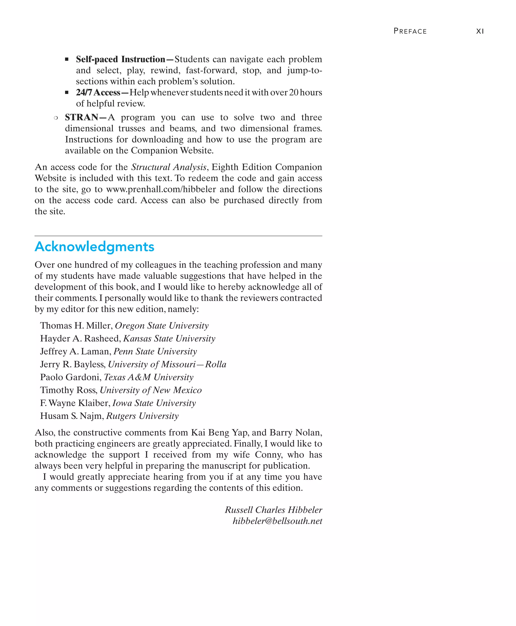
182 CHAPTER 5 CABLES AND ARCHES
When deriving the necessary relations between the force in the cable
and its slope, we will make the assumption that the cable is perfectly
flexible and inextensible. Due to its flexibility, the cable offers no
resistance to shear or bending and, therefore, the force acting in the
cable is always tangent to the cable at points along its length. Being
inextensible, the cable has a constant length both before and after the
load is applied.As a result, once the load is applied, the geometry of the
cable remains fixed, and the cable or a segment of it can be treated as a
rigid body.
5.2 Cable Subjected to Concentrated
Loads
When a cable of negligible weight supports several concentrated loads,
the cable takes the form of several straight-line segments, each of which
is subjected to a constant tensile force. Consider, for example, the cable
shown in Fig. 5–1. Here specifies the angle of the cable’s cord AB,
and L is the cable’s span. If the distances and and the loads
and are known, then the problem is to determine the nine
unknowns consisting of the tension in each of the three segments, the
four components of reaction at A and B, and the sags and at
the two points C and D. For the solution we can write two equations of
force equilibrium at each of points A, B, C, and D. This results in a total
of eight equations. To complete the solution, it will be necessary to know
something about the geometry of the cable in order to obtain the
necessary ninth equation. For example, if the cable’s total length
is specified, then the Pythagorean theorem can be used to relate to
each of the three segmental lengths, written in terms of
and Unfortunately, this type of problem cannot be solved easily by
hand. Another possibility, however, is to specify one of the sags, either
or instead of the cable length. By doing this, the equilibrium
equations are then sufficient for obtaining the unknown forces and the
remaining sag. Once the sag at each point of loading is obtained, can
then be determined by trigonometry.
When performing an equilibrium analysis for a problem of this type,
the forces in the cable can also be obtained by writing the equations of
equilibrium for the entire cable or any portion thereof. The following
example numerically illustrates these concepts.
l
yD,
yC
L3.
L2,
L1,
yD,
yC,
u,
l
l
yD
yC
P2
P1
L3
L2,
L1,
u
5
yC yD
C
D
A
B
L1 L2 L3
L
P1
P2
u
Fig. 5–1

5.2 CABLE SUBJECTED TO CONCENTRATED LOADS 183
5
EXAMPLE 5.1
Determine the tension in each segment of the cable shown in Fig. 5–2a.
Also, what is the dimension h?
SOLUTION
By inspection, there are four unknown external reactions (
and ) and three unknown cable tensions, one in each cable segment.
These seven unknowns along with the sag h can be determined from
the eight available equilibrium equations
applied to points A through D.
A more direct approach to the solution is to recognize that the slope
of cable CD is specified, and so a free-body diagram of the entire cable
is shown in Fig. 5–2b. We can obtain the tension in segment CD as
follows:
Ans.
Now we can analyze the equilibrium of points C and B in sequence.
Point C (Fig. 5–2c);
Ans.
Point B (Fig. 5–2d);
Ans.
Hence, from Fig. 5–2a,
Ans.
h = 12 m2 tan 53.8° = 2.74 m
uBA = 53.8° TBA = 6.90 kN
TBA sin uBA - 4.82 kN sin 32.3° - 3 kN = 0
+ c©Fy = 0;
-TBA cos uBA + 4.82 kN cos 32.3° = 0
:
+ ©Fx = 0;
uBC = 32.3° TBC = 4.82 kN
6.79 kN1452 - 8 kN + TBC sin uBC = 0
+ c©Fy = 0;
6.79 kN1352 - TBC cos uBC = 0
:
+ ©Fx = 0;
TCD = 6.79 kN
TCD135212 m2 + TCD145215.5 m2 - 3 kN12 m2 - 8 kN14 m2 = 0
d+©MA = 0;
1©Fx = 0, ©Fy = 02
Dy
Dx,
Ay,
Ax,
Fig. 5–2
y
x
C
TBC
6.79 kN
uBC
8 kN
(c)
3
4
5
y
x
B
TBA
uBA
3 kN
(d)
4.82 kN
32.3
2 m
3 kN
8 kN
2 m 1.5 m
2 m
2 m
h
A
B
C
(a)
D
2 m
3 kN
8 kN
2 m
2 m
A
B
C
D
(b)
TCD
Ay
Ax
1.5 m
3
4
5

5.3 Cable Subjected to a Uniform
Distributed Load
Cables provide a very effective means of supporting the dead weight of
girders or bridge decks having very long spans. A suspension bridge is a
typical example, in which the deck is suspended from the cable using a
series of close and equally spaced hangers.
In order to analyze this problem, we will first determine the shape of a
cable subjected to a uniform horizontally distributed vertical load
Fig. 5–3a. Here the x,y axes have their origin located at the lowest point
on the cable, such that the slope is zero at this point. The free-body
diagram of a small segment of the cable having a length is shown in
Fig. 5–3b. Since the tensile force in the cable changes continuously in
both magnitude and direction along the cable’s length, this change is
denoted on the free-body diagram by The distributed load is
represented by its resultant force which acts at from point O.
Applying the equations of equilibrium yields
Dividing each of these equations by and taking the limit as
and hence and we obtain
(5–1)
(5–2)
(5–3)
Integrating Eq. 5–1, where at we have:
(5–4)
which indicates the horizontal component of force at any point along the
cable remains constant.
Integrating Eq. 5–2, realizing that at gives
(5–5)
Dividing Eq. 5–5 by Eq. 5–4 eliminates T. Then using Eq. 5–3, we can
obtain the slope at any point,
(5–6)
tan u =
dy
dx
=
w0x
FH
T sin u = w0x
x = 0,
T sin u = 0
T cos u = FH
x = 0,
T = FH
dy
dx
= tan u
d1T sin u2
dx
= w0
d1T cos u2
dx
= 0
¢T : 0,
¢u : 0,
¢y : 0,
¢x : 0,
¢x
w01¢x21¢x22 - T cos u ¢y + T sin u ¢x = 0
d+©MO = 0;
-T sin u - w01¢x2 + 1T + ¢T2 sin1u + ¢u2 = 0
+ c©Fy = 0;
-T cos u + 1T + ¢T2 cos1u + ¢u2 = 0
:
+ ©Fx = 0;
¢x2
w0¢x,
¢T.
¢s
w0,
5
Fig. 5–3
w0
L
x x
h
(a)
x
y
x
s
T
O
T T
y
x
–––
2
w0(x)
(b)
u u
u

5.3 CABLE SUBJECTED TO A UNIFORM DISTRIBUTED LOAD 185
5
Performing a second integration with at yields
(5–7)
This is the equation of a parabola. The constant may be obtained by
using the boundary condition at Thus,
(5–8)
Finally, substituting into Eq. 5–7 yields
(5–9)
From Eq. 5–4, the maximum tension in the cable occurs when is
maximum; i.e., at Hence, from Eqs. 5–4 and 5–5,
(5–10)
Or, using Eq. 5–8, we can express in terms of i.e.,
(5–11)
Realize that we have neglected the weight of the cable, which is
uniform along the length of the cable, and not along its horizontal
projection. Actually, a cable subjected to its own weight and free of any
other loads will take the form of a catenary curve. However, if the sag-to-
span ratio is small, which is the case for most structural applications, this
curve closely approximates a parabolic shape, as determined here.
From the results of this analysis, it follows that a cable will maintain a
parabolic shape, provided the dead load of the deck for a suspension
bridge or a suspended girder will be uniformly distributed over the
horizontal projected length of the cable. Hence, if the girder in Fig. 5–4a
is supported by a series of hangers, which are close and uniformly
spaced, the load in each hanger must be the same so as to ensure that the
cable has a parabolic shape.
Using this assumption, we can perform the structural analysis of the
girder or any other framework which is freely suspended from the cable.
In particular, if the girder is simply supported as well as supported by
the cable, the analysis will be statically indeterminate to the first degree,
Fig. 5–4b. However, if the girder has an internal pin at some intermediate
point along its length, Fig. 5–4c, then this would provide a condition of
zero moment, and so a determinate structural analysis of the girder can
be performed.
Tmax = w0L21 + 1L2h22
w0,
Tmax
Tmax = 2FH
2
+ 1w0L22
x = L.
u
y =
h
L2
x2
FH =
w0L2
2h
x = L.
y = h
FH
y =
w0
2FH
x2
x = 0
y = 0
Fig. 5–4
(a)
(b)
(c)
The Verrazano-Narrows Bridge at the
entrance to New York Harbor has a main
span of 4260 ft (1.30 km).

5
Fig. 5–5
The cable in Fig. 5–5a supports a girder which weighs .
Determine the tension in the cable at points A, B, and C.
850 lbft
EXAMPLE 5.2
C
100 ft
20 ft
(a)
A
B
40 ft
(b)
100 ft x¿
40 ft
20 ft
A
C
B
y
x¿
x
SOLUTION
The origin of the coordinate axes is established at point B, the lowest
point on the cable, where the slope is zero, Fig. 5–5b. From Eq. 5–7, the
parabolic equation for the cable is:
(1)
Assuming point C is located from B, we have
(2)
Also, for point A,
x¿ = 41.42 ft
xœ2
+ 200x¿ - 10 000 = 0
40 =
425
21.25xœ2
[-1100 - x¿2]2
40 =
425
FH
[-1100 - x¿2]2
FH = 21.25xœ2
20 =
425
FH
xœ2
x¿
y =
w0
2FH
x2
=
850 lbft
2FH
x2
=
425
FH
x2

5
Thus, from Eqs. 2 and 1 (or Eq. 5–6) we have
(3)
At point A,
Using Eq. 5–4,
Ans.
At point B,
Ans.
At point C,
Ans.
TC =
FH
cos uC
=
36 459.2
cos 44.0°
= 50.7 k
uC = 44.0°
tan uC =
dy
dx
`
x=41.42
= 0.02331141.422 = 0.9657
x = 41.42 ft
TB =
FH
cos uB
=
36 459.2
cos 0°
= 36.5 k
tan uB =
dy
dx
`
x=0
= 0, uB = 0°
x = 0,
TA =
FH
cos uA
=
36 459.2
cos1-53.79°2
= 61.7 k
uA = -53.79°
tan uA =
dy
dx
`
x= -58.58
= 0.023311-58.582 = -1.366
x = -1100 - 41.422 = -58.58 ft
dy
dx
=
850
36 459.2
x = 0.02331x
FH = 21.25141.4222
= 36 459.2 lb

5
Fig. 5–6
The suspension bridge in Fig. 5–6a is constructed using the two
stiffening trusses that are pin connected at their ends C and supported
by a pin at A and a rocker at B. Determine the maximum tension in
the cable IH. The cable has a parabolic shape and the bridge is
subjected to the single load of 50 kN.
SOLUTION
The free-body diagram of the cable-truss system is shown in Fig. 5–6b.
According to Eq. 5–4 the horizontal component of
cable tension at I and H must be constant, Taking moments about
B, we have
Iy + Ay = 18.75
-Iy124 m2 - Ay124 m2 + 50 kN19 m2 = 0
d+©MB = 0;
FH.
1T cos u = FH2,
EXAMPLE 5.3
50 kN
A
D
F G C
B
E
4 @ 3 m 12 m 4 @ 3 m 12 m
8 m
6 m
(a)
I H
50 kN
24 m
(b)
Ay By
9 m
FH FH
Iy
Hy
Ax
B

5
If only half the suspended structure is considered, Fig. 5–6c, then
summing moments about the pin at C, we have
From these two equations,
To obtain the maximum tension in the cable, we will use Eq. 5–11, but
first it is necessary to determine the value of an assumed uniform
distributed loading from Eq. 5–8:
Thus, using Eq. 5–11, we have
Ans.
= 46.9 kN
= 3.125112 m221 + 112 m218 m222
Tmax = w0L21 + 1L2h22
w0 =
2FHh
L2
=
2128.125 kN218 m2
112 m22
= 3.125 kNm
w0
FH = 28.125 kN
18.75 = 0.667FH
Iy + Ay = 0.667FH
FH114 m2 - FH16 m2 - Iy112 m2 - Ay112 m2 = 0
d+©MC = 0;
12 m
6 m
14 m
C
(c)
Ay
FH
FH
Cx
Cy
Iy
Ax

5
Prob. 5–1
Prob. 5–2
Prob. 5–3
Probs. 5–4/5–5
5–1. Determine the tension in each segment of the cable
and the cable’s total length.
5–3. Determine the tension in each cable segment and the
distance yD.
PROBLEMS
5–2. Cable ABCD supports the loading shown. Determine
the maximum tension in the cable and the sag of point B.
*5–4. The cable supports the loading shown.Determine the
distance the force at point B acts from A. Set .
5–5. The cable supports the loading shown. Determine the
magnitude of the horizontal force P so that .
xB = 6 ft
P = 40 lb
xB
7 m
B
A
D
C
4 m 5 m 3 m
2 kN
4 kN
yD
2 m
5 ft
2 ft
3 ft
30 lb
D
C
B
A
xB
5
4
3
8 ft
P
1 m
A
B
C
D
yB 2 m
3 m
4 kN 6 kN
0.5 m
4 ft 5 ft
A
3 ft
B
7 ft
4 ft
C
D
50 lb
100 lb

5
Prob. 5–6
5–7. The cable is subjected to the uniform loading. If the
slope of the cable at point O is zero, determine the equation
of the curve and the force in the cable at O and B.
5–9. Determine the maximum and minimum tension in the
cable.
5–6. Determine the forces and needed to hold the
cable in the position shown, i.e., so segment CD remains
horizontal.Also find the maximum loading in the cable.
P2
P1 *5–8. The cable supports the uniform load of
Determine the tension in the cable at each
support A and B.
w0 = 600 lbft.
Prob. 5–7
Prob. 5–8
Prob. 5–9
A
P1 P2
5 kN
1.5 m
1 m
B
C D
E
4 m 4 m
5 m
2 m
15 ft
8 ft
y
x
A
O
B
15 ft
500 lb/ft
15 ft
A
B
10 ft
25 ft
w0
10 m
16 kN/m
2 m
y
x
A B
10 m

5
Prob. 5–10
Prob. 5–12
Prob. 5–13
Probs. 5–14/5–15
5–10. Determine the maximum uniform loading w,
measured in , that the cable can support if it is capable
of sustaining a maximum tension of 3000 lb before it will
break.
lbft
5–13. The trusses are pin connected and suspended from
the parabolic cable. Determine the maximum force in the
cable when the structure is subjected to the loading shown.
*5–12. The cable shown is subjected to the uniform load .
Determine the ratio between the rise h and the span L that
will result in using the minimum amount of material for the
cable.
w0
5–14. Determine the maximum and minimum tension in
the parabolic cable and the force in each of the hangers.The
girder is subjected to the uniform load and is pin connected
at B.
5–15. Draw the shear and moment diagrams for the pin-
connected girders AB and BC. The cable has a parabolic
shape.
A
D
B
C
E
30 ft
9 ft
1 ft
10 ft
10 ft
2 k/ft
4 k
5 k
A
F G H B
C
I
J
K
16 ft
4 @ 12 ft 48 ft 4 @ 12 ft 48 ft
D E
6 ft
14 ft
50 ft
6 ft
w
Prob. 5–11
50 ft
6 ft
w
L
h
w0
5–11. The cable is subjected to a uniform loading of
. Determine the maximum and minimum
tension in the cable.
w = 250 lb ft

5
A
B
2 m
3 kN 5 kN
C
F
D
E
2 m 2 m 2 m 2 m 2 m 2 m 2 m
9 m
3 m 3 m
*5–16. The cable will break when the maximum tension
reaches . Determine the maximum uni-
form distributed load w required to develop this maximum
tension.
5–17. The cable is subjected to a uniform loading of
kN/m. Determine the maximum and minimum
tension in cable.
w = 60
Tmax = 5000 kN
5–19. The beams AB and BC are supported by the cable
that has a parabolic shape. Determine the tension in the cable
at points D, F, and E, and the force in each of the equally
spaced hangers.
5–18. The cable AB is subjected to a uniform loading of
. If the weight of the cable is neglected and the
slope angles at points A and B are and , respectively,
determine the curve that defines the cable shape and the
maximum tension developed in the cable.
60°
30°
200 Nm
*5–20. Draw the shear and moment diagrams for beams
AB and BC.The cable has a parabolic shape.
Prob. 5–20
Probs. 5–16/5–17
Prob. 5–18
Prob. 5–19
15 m
200 N/m
y
x
A
B
60
30
100 m
12 m
w
A
B
2 m
3 kN 5 kN
C
F
D
E
2 m 2 m 2 m 2 m 2 m 2 m 2 m
9 m
3 m 3 m

5.4 Arches
Like cables, arches can be used to reduce the bending moments in
long-span structures. Essentially, an arch acts as an inverted cable, so it
receives its load mainly in compression although, because of its rigidity, it
must also resist some bending and shear depending upon how it is loaded
and shaped. In particular, if the arch has a parabolic shape and it is
subjected to a uniform horizontally distributed vertical load, then from the
analysis of cables it follows that only compressive forces will be resisted by
the arch. Under these conditions the arch shape is called a funicular arch
because no bending or shear forces occur within the arch.
A typical arch is shown in Fig. 5–7, which specifies some of the nomen-
clature used to define its geometry. Depending upon the application,
several types of arches can be selected to support a loading.A fixed arch,
Fig. 5–8a, is often made from reinforced concrete. Although it may
require less material to construct than other types of arches, it must have
solid foundation abutments since it is indeterminate to the third degree
and, consequently, additional stresses can be introduced into the arch
due to relative settlement of its supports.A two-hinged arch, Fig. 5–8b, is
commonly made from metal or timber. It is indeterminate to the first
degree, and although it is not as rigid as a fixed arch, it is somewhat
insensitive to settlement. We could make this structure statically
determinate by replacing one of the hinges with a roller. Doing so,
however, would remove the capacity of the structure to resist bending
along its span, and as a result it would serve as a curved beam, and not as
an arch.A three-hinged arch, Fig. 5–8c, which is also made from metal or
timber, is statically determinate. Unlike statically indeterminate arches,
it is not affected by settlement or temperature changes. Finally, if two-
and three-hinged arches are to be constructed without the need for
larger foundation abutments and if clearance is not a problem, then the
supports can be connected with a tie rod, Fig. 5–8d. A tied arch allows
the structure to behave as a rigid unit, since the tie rod carries the
horizontal component of thrust at the supports. It is also unaffected by
relative settlement of the supports.
5
Fig. 5–7
extrados
(or back)
abutment
intrados
(or soffit)
haunch
centerline rise
springline
crown
(a)
fixed arch
(b)
two-hinged arch
(d)
tied arch
(c)
three-hinged arch
Fig. 5–8

5.5 THREE-HINGED ARCH 195
5
5.5 Three-Hinged Arch
To provide some insight as to how arches transmit loads, we will now
consider the analysis of a three-hinged arch such as the one shown in
Fig. 5–9a. In this case, the third hinge is located at the crown and the
supports are located at different elevations. In order to determine the
reactions at the supports, the arch is disassembled and the free-body
diagram of each member is shown in Fig. 5–9b. Here there are six
unknowns for which six equations of equilibrium are available. One
method of solving this problem is to apply the moment equilibrium
equations about points A and B. Simultaneous solution will yield the
reactions and The support reactions are then determined from
the force equations of equilibrium. Once obtained, the internal normal
force, shear, and moment loadings at any point along the arch can be
found using the method of sections. Here, of course, the section should
be taken perpendicular to the axis of the arch at the point considered. For
example, the free-body diagram for segment AD is shown in Fig. 5–9c.
Three-hinged arches can also take the form of two pin-connected
trusses, each of which would replace the arch ribs AC and CB in Fig. 5–9a.
The analysis of this form follows the same procedure outlined above.The
following examples numerically illustrate these concepts.
Cy.
Cx
(a)
A
C
B
D
P1
P2
(b)
P1
P2
Ax
Ay
Cy
Cx
Cx
Cy
By
Bx
Ax
Ay
(c)
VD
ND
MD
Fig. 5–9
(b)
The three-hinge truss arch is used to support
a portion of the roof loading of this building
(a). The close-up photo shows the arch is
pinned at its top (b).
(a)

Fig. 5–10
5
The three-hinged open-spandrel arch bridge like the one shown in the
photo has a parabolic shape. If this arch were to support a uniform
load and have the dimensions shown in Fig. 5–10a, show that the arch
is subjected only to axial compression at any intermediate point such
as point D. Assume the load is uniformly transmitted to the arch ribs.
EXAMPLE 5.4
SOLUTION
Here the supports are at the same elevation. The free-body diagrams
of the entire arch and part BC are shown in Fig. 5–10b and Fig. 5–10c.
Applying the equations of equilibrium, we have:
Entire arch:
Cy = 25 k
Cy1100 ft2 - 50 k150 ft2 = 0
d+©MA = 0;
A
B
C
y
50 ft 25 ft 25 ft
25 ft
x
500 lb/ft
y x2
(50)2
(a)
D
25
Ay
B
50 ft 50 ft
50 k
(b)
Ax
Cy
Cx

5
Arch segment BC:
A section of the arch taken through point D,
is shown in Fig. 5–10d. The slope of
the segment at D is
Applying the equations of equilibrium, Fig. 5–10d we have
Ans.
Ans.
Ans.
Note: If the arch had a different shape or if the load were nonuniform, then the internal
shear and moment would be nonzero. Also, if a simply supported beam were used to
support the distributed loading, it would have to resist a maximum bending moment of
By comparison, it is more efficient to structurally resist the load in direct
compression (although one must consider the possibility of buckling) than to resist the
load by a bending moment.
M = 625 k # ft.
MD = 0
VD = 0
ND = 28.0 k
MD + 12.5 k112.5 ft2 - 25 k16.25 ft2 = 0
d+©MD = 0;
-12.5 k + ND sin 26.6° - VD cos 26.6° = 0
+ c©Fy = 0;
25 k - ND cos 26.6° - VD sin 26.6° = 0
:
+ ©Fx = 0;
u = -26.6°
tan u =
dy
dx
=
-50
15022
x `
x=25 ft
= -0.5
y = -2512522
15022
= -6.25 ft,
x = 25 ft,
By = 0
By - 25 k + 25 k = 0
+ c©Fy = 0;
Bx = 25 k
:
+ ©Fx = 0;
Cx = 25 k
-25 k125 ft2 + 25 k150 ft2 - Cx125 ft2 = 0
d+©MB = 0;
25 ft
25 k
(c)
Cy
Cx
25 ft
25 ft
By
Bx
B
12.5 ft
12.5 k
(d)
B
D
12.5 ft
26.6
ND
26.6
VD
MD
25 k
6.25 ft

5
Fig. 5–11
The three-hinged tied arch is subjected to the loading shown in
Fig. 5–11a. Determine the force in members CH and CB. The dashed
member GF of the truss is intended to carry no force.
EXAMPLE 5.5
SOLUTION
The support reactions can be obtained from a free-body diagram of
the entire arch, Fig. 5–11b:
A
15 kN
20 kN
15 kN
E
(b)
Ay
Ax
Ey
3 m 3 m 3 m 3 m
4 m
1 m
1 m
A
3 m 3 m 3 m 3 m
B
H
D
F
G
15 kN 20 kN
15 kN
C
E
(a)
Ey112 m2 - 15 kN13 m2 - 20 kN16 m2 - 15 kN19 m2 = 0
d+©MA = 0;
5 m
3 m 3 m
15 kN 20 kN
(c)
Cx
Cy
25 kN
FAE
0
C
The force components acting at joint C can be determined by consid-
ering the free-body diagram of the left part of the arch, Fig. 5–11c.
First, we determine the force:
FAE = 21.0 kN
FAE15 m2 - 25 kN16 m2 + 15 kN13 m2 = 0
d+©MC = 0;
Ay = 25 kN
Ay - 15 kN - 20 kN - 15 kN + 25 kN = 0
+c ©Fy = 0;
Ax = 0
:
+ ©Fx = 0;
Ey = 25 kN

5
Then,
To obtain the forces in CH and CB, we can use the method of joints
as follows:
Joint G; Fig. 5–11d,
Joint C; Fig. 5–11e,
Thus,
Ans.
Ans.
FCH = 4.74 kN 1T2
FCB = 26.9 kN 1C2
FCBA 1
110 B + FCHA 1
110 B - 20 kN + 10 kN = 0
+ c©Fy = 0;
FCBA 3
110 B - 21.0 kN - FCHA 3
110 B = 0
:
+ ©Fx = 0;
FGC = 20 kN 1C2
FGC - 20 kN = 0
+ c©Fy = 0;
25 kN - 15 kN - 20 kN + Cy = 0, Cy = 10 kN
+ c©Fy = 0;
-Cx + 21.0 kN = 0, Cx = 21.0 kN
:
+ ©Fx = 0;
FGC
FHG 0
20 kN
(d)
G
FCH
20 kN
3
1
FCB
10 kN
3
1
21.0 kN
(e)
C
Note: Tied arches are sometimes used for
bridges. Here the deck is supported by
suspender bars that transmit their load to
the arch. The deck is in tension so that it
supports the actual thrust or horizontal
force at the ends of the arch.

5
10 ft 10 ft
15 ft
yD
y cx2
x
y
C
D
E
Fig. 5–12
The three-hinged trussed arch shown in Fig. 5–12a supports the
symmetric loading. Determine the required height of the joints B
and D, so that the arch takes a funicular shape. Member HG is
intended to carry no force.
h1
EXAMPLE 5.6
SOLUTION
For a symmetric loading, the funicular shape for the arch must be
parabolic as indicated by the dashed line (Fig. 5–12b). Here we must
find the equation which fits this shape. With the x, y axes having an
origin at C, the equation is of the form To obtain the
constant c, we require
Therefore,
So that from Fig. 5–12a,
Ans.
Using this value, if the method of joints is now applied to the truss, the
results will show that the top cord and diagonal members will all be
zero-force members, and the symmetric loading will be supported
only by the bottom cord members AB, BC, CD, and DE of the truss.
h1 = 15 ft - 3.75 ft = 11.25 ft
yD = -10.0375ft2110 ft22
= -3.75 ft
c = 0.0375ft
-115 ft2 = -c120 ft22
y = -cx2
.
(b)
5 k 5 k 5 k 5 k
I
J
B
C
D
A
H G F
E
5 k
(a)
10 ft 10 ft
15 ft
h1 h1
10 ft 10 ft

5
5–21. The tied three-hinged arch is subjected to the
loading shown. Determine the components of reaction at
A and C and the tension in the cable.
5–23. The three-hinged spandrel arch is subjected to the
loading shown. Determine the internal moment in the arch
at point D.
PROBLEMS
5–22. Determine the resultant forces at the pins A, B, and
C of the three-hinged arched roof truss.
*5–24. The tied three-hinged arch is subjected to the
loading shown. Determine the components of reaction
A and C, and the tension in the rod.
3 m
5 m
3 m 3 m
1 m 1 m
2 m 2 m
B
C
A
2 kN
3 kN
4 kN 4 kN
5 kN
10 kN
15 kN
2 m
2 m
0.5 m
2 m 1 m
A
B
C
Prob. 5–21
Prob. 5–22
Prob. 5–23
Prob. 5–24
A
B
C
3 m
4 kN
8 kN 8 kN
4 kN 3 kN
6 kN 6 kN
3 kN
5 m
2 m 2 m 2 m 2 m 2 m 2 m
3 m 5 m 8 m
D
A
C
B
4 k
3 k
5 k
6 ft 6 ft
8 ft 10 ft 10 ft
15 ft

5
Probs. 5–25/5–26
Prob. 5–27
Prob. 5–28
Prob. 5–29
30 ft 30 ft
30 ft 30 ft 30 ft
10 ft
D E
20 k
20 k
60 k 40 k
40 k
B
A C
100 ft
30 ft
h1
h2
h3
30 ft 30 ft
5–25. The bridge is constructed as a three-hinged trussed
arch. Determine the horizontal and vertical components of
reaction at the hinges (pins) at A, B, and C. The dashed
member DE is intended to carry no force.
5–26. Determine the design heights and of the
bottom cord of the truss so the three-hinged trussed arch
responds as a funicular arch.
h3
h2,
h1,
*5–28. The three-hinged spandrel arch is subjected to the
uniform load of 20 kN兾m. Determine the internal moment
in the arch at point D.
of reaction at A, B, and C of the three-hinged arch.Assume
A, B, and C are pin connected.
5–29. The arch structure is subjected to the loading
shown. Determine the horizontal and vertical components
of reaction at A and D, and the tension in the rod AD.
E
C
2 k/ft
A
B
D
8 ft
3 k
4 ft 4 ft 6 ft
3 ft
3 ft
A C
D
B
5 m
3 m
3 m 8 m
20 kN/m
5 m
5 ft
8 ft
A
C
B
4 k
3 k 2 ft

5
CHAPTER REVIEW
Cables support their loads in tension if we consider them
perfectly flexible.
If the cable is subjected to concentrated loads then the
force acting in each cable segment is determined by
applying the equations of equilibrium to the free-body
diagram of groups of segments of the cable or to the joints
where the forces are applied.
If the cable supports a uniform load over a projected
horizontal distance, then the shape of the cable takes the
form of a parabola.
Arches are designed primarily to carry a compressive force.
A parabolic shape is required to support a uniform loading
distributed over its horizontal projection.
Three-hinged arches are statically determinate and can be
analyzed by separating the two members and applying the
equations of equilibrium to each member.
L1 L2 L3
L
P1
P2
w0
L
h
x
y
three-hinged arch
CHAPTER REVIEW 203

Moving loads caused by trains must be considered when designing the
members of this bridge. The influence lines for the members become an
important part of the structural analysis.

6
205
Influence lines have important application for the design of structures
that resist large live loads. In this chapter we will discuss how to draw
the influence line for a statically determinate structure. The theory is
applied to structures subjected to a distributed load or a series of
concentrated forces, and specific applications to floor girders and
bridge trusses are given. The determination of the absolute maximum
live shear and moment in a member is discussed at the end of
the chapter.
6.1 Influence Lines
In the previous chapters we developed techniques for analyzing the
forces in structural members due to dead or fixed loads. It was shown
that the shear and moment diagrams represent the most descriptive
methods for displaying the variation of these loads in a member. If a
structure is subjected to a live or moving load, however, the variation of
the shear and bending moment in the member is best described using
the influence line. An influence line represents the variation of either the
reaction, shear, moment, or deflection at a specific point in a member
as a concentrated force moves over the member. Once this line is
constructed, one can tell at a glance where the moving load should be
placed on the structure so that it creates the greatest influence at the
specified point. Furthermore, the magnitude of the associated reaction,
shear, moment, or deflection at the point can then be calculated from the
ordinates of the influence-line diagram. For these reasons, influence lines
play an important part in the design of bridges, industrial crane rails,
conveyors, and other structures where loads move across their span.
Influence Lines for
Statically Determinate
Structures

206 CHAPTER 6 INFLUENCE LINES FOR STATICALLY DETERMINATE STRUCTURES
6
Either of the following two procedures can be used to construct the
influence line at a specific point P in a member for any function
(reaction, shear, or moment). For both of these procedures we will
choose the moving force to have a dimensionless magnitude of unity.*
Tabulate Values
• Place a unit load at various locations, x, along the member, and
at each location use statics to determine the value of the function
(reaction, shear, or moment) at the specified point.
• If the influence line for a vertical force reaction at a point on a
beam is to be constructed, consider the reaction to be positive at
the point when it acts upward on the beam.
• If a shear or moment influence line is to be drawn for a point, take
the shear or moment at the point as positive according to the same
sign convention used for drawing shear and moment diagrams.
(See Fig. 4–1.)
• All statically determinate beams will have influence lines that
consist of straight line segments. After some practice one should
be able to minimize computations and locate the unit load only at
points representing the end points of each line segment.
• To avoid errors, it is recommended that one first construct a table,
listing “unit load at x” versus the corresponding value of the
function calculated at the specific point; that is, “reaction R,”
“shear V,” or “moment M.” Once the load has been placed at
various points along the span of the member, the tabulated values
can be plotted and the influence-line segments constructed.
Influence-Line Equations
• The influence line can also be constructed by placing the unit load
at a variable position x on the member and then computing the
value of R, V, or M at the point as a function of x. In this manner,
the equations of the various line segments composing the
influence line can be determined and plotted.
Although the procedure for constructing an influence line is rather
basic, one should clearly be aware of the difference between constructing
an influence line and constructing a shear or moment diagram. Influence
lines represent the effect of a moving load only at a specified point on a
member, whereas shear and moment diagrams represent the effect of
fixed loads at all points along the axis of the member.
*The reason for this choice will be explained in Sec. 6–2.

6.1 INFLUENCE LINES 207
6
EXAMPLE 6.1
Construct the influence line for the vertical reaction at A of the beam
in Fig. 6–1a.
SOLUTION
Tabulate Values. A unit load is placed on the beam at each selected
point x and the value of is calculated by summing moments about B.
For example, when and see Figs. 6–1b and 6–1c,
respectively.The results for are entered in the table, Fig. 6–1d.A plot
of these values yields the influence line for the reaction at A, Fig. 6–1e.
Ay
x = 5 ft,
x = 2.5 ft
Ay
(a)
A
B
10 ft
10 ft
(b)
Ay
1
By
x 2.5 ft
兺MB 0; Ay (10) 1 (7.5) 0
Ay 0.75
x 5 ft
10 ft
(c)
Ay
1
By
兺MB 0; Ay (10) 1 (5) 0
Ay 0.5
1
0.75
0.5
0.25
0
(d)
x Ay
0
2.5
5
7.5
10
(e)
Ay
x
10
1
Ay 1 __ x
10
1
influence line for Ay
x
10 ft
(f)
Ay
1
By
Influence-Line Equation. When the unit load is placed a variable
distance x from A, Fig. 6–1f, the reaction as a function of x can be
determined from
This line is plotted in Fig. 6–1e.
Ay = 1 - 1
10 x
-Ay1102 + 110 - x2112 = 0
d+©MB = 0;
Ay
Fig. 6–1

6
Construct the influence line for the vertical reaction at B of the beam
in Fig. 6–2a.
EXAMPLE 6.2
SOLUTION
Tabulate Values. Using statics, verify that the values for the reaction
listed in the table, Fig. 6–2b, are correctly computed for each
position x of the unit load. A plot of the values yields the influence
line in Fig. 6–2c.
By
Influence-Line Equation. Applying the moment equation about A,
in Fig. 6–2d,
This is plotted in Fig. 6–2c.
By = 1
5 x
By152 - 11x2 = 0
d+©MA = 0;
(a)
A B
5 m 5 m
x
1
0
0.5
1
1.5
2
(b)
x By
0
2.5
5
7.5
10
By
2
1
By __ x
5
x
10
(c)
influence line for By
A B
x
5 m 5 m
(d)
Ay By
1
Fig. 6–2

6
EXAMPLE 6.3
Construct the influence line for the shear at point C of the beam in
Fig. 6–3a.
SOLUTION
Tabulate Values. At each selected position x of the unit load,
the method of sections is used to calculate the value of Note in
particular that the unit load must be placed just to the left
and just to the right of point C since the shear is discontinu-
ous at C, Figs. 6–3b and 6–3c. A plot of the values in Fig. 6–3d yields
the influence line for the shear at C, Fig. 6–3e.
1x = 2.5+
2
1x = 2.5-
2
VC.
Influence-Line Equations. Here two equations have to be determined
since there are two segments for the influence line due to the
discontinuity of shear at C, Fig. 6–3f. These equations are plotted in
Fig. 6–3e.
2.5 ft
10 ft
C
(a)
A
B
0.75
C 10 ft
(b)
1
2.5
ft
0.25
MC
VC
兺Fy 0; VC 0.25
0.25 0.75
C 10 ft
(c)
1
1
2.5
ft
0.25
MC
VC
兺Fy 0; VC 0.75
0.25
(d)
x VC
0
2.5
2.5
5
7.5
10
0
0.25
0.75
0.5
0.25
0
VC
0.75
2.5
–0.25
10
x
(e)
influence line for VC
1
VC 1 __ x
10
1
VC __ x
10
x
(f)
0 x 2.5 ft
x
1
MC
VC
2.5 ft
MC
VC
2.5 ft
1
By
2.5 ft x 10 ft
1
Ay 1 __ x
10
1
Ay 1 __ x
10
Fig. 6–3

6
Construct the influence line for the shear at point C of the beam in
Fig. 6–4a.
SOLUTION
Tabulate Values. Using statics and the method of sections, verify
that the values of the shear at point C in Fig. 6–4b correspond to
each position x of the unit load on the beam. A plot of the values in
Fig. 6–4b yields the influence line in Fig. 6–4c.
VC
EXAMPLE 6.4
Influence-Line Equations. From Fig. 6–4d, verify that
These equations are plotted in Fig. 6–4c.
VC = 1 - 1
8 x 4 m 6 x … 12 m
VC = -1
8 x 0 … x 6 4 m
C
4 m 4 m 4 m
B
(a)
1
x
A
(b)
x VC
0
4
4
8
12
0
0.5
0.5
0
0.5
0.5
0.5
0.5
VC
4
8
1
VC 1 __ x
8
1
VC __ x
8
12
x
(c)
(d)
0 x 4 m
x
1
MC
VC
4 m
Ay 1 x
1
__
8
x
MC
VC
4 m
Ay 1 x
1
__
8
1
By
4 m x 12 m
Fig. 6–4

6
EXAMPLE 6.5
Construct the influence line for the moment at point C of the beam in
Fig. 6–5a.
SOLUTION
Tabulate Values. At each selected position of the unit load, the value
of is calculated using the method of sections. For example, see
Fig. 6–5b for A plot of the values in Fig. 6–5c yields the
influence line for the moment at C, Fig. 6–5d.
x = 2.5 ft.
MC
Influence-Line Equations. The two line segments for the influence
line can be determined using along with the method of
sections shown in Fig. 6–5e. These equations when plotted yield the
influence line shown in Fig. 6–5d.
©MC = 0
5 ft 6 x … 10 ft
MC = 5 - 1
2x
0 … x 6 5 ft
MC = 1
2x
MC - A1 - 1
10 xB5 = 0
MC + 115 - x2 - A1 - 1
10 xB5 = 0 d+©MC = 0;
d+©MC = 0;
10 ft
5 ft
A C
B
(a)
(b)
C
0.25
0.75
5 ft
MC
VC
兺MC 0; MC 0.25 (5) 0
MC 1.25
1
2.5 ft
0.25
(c)
x MC
0
2.5
5
7.5
10
0
1.25
2.5
1.25
0
MC
5 10
x
2.5
(d)
influence line for MC
1
MC 5 __ x
2
1
MC __ x
2
(e)
x
1
MC
VC
5 ft
1
Ay 1 __ x
10
x MC
VC
5 ft
1
By
1
Ay 1 __ x
10
Fig. 6–5

6
Construct the influence line for the moment at point C of the beam in
Fig. 6–6a.
EXAMPLE 6.6
SOLUTION
Tabulate Values. Using statics and the method of sections, verify
that the values of the moment at point C in Fig. 6–6b correspond
to each position x of the unit load. A plot of the values in Fig. 6–6b
yields the influence line in Fig. 6–6c.
MC
C
(a)
B
4 m 4 m 4 m
1
x
A
(b)
x MC
0
4
8
12
0
2
0
2
2
4
8 12
MC
2
x
(c)
(d)
0 x 4 m
x
1
MC
VC
4 m
x
MC
VC
4 m
1
By
4 m x 12 m
1
Ay 1 __ x
8
1
Ay 1 __ x
8
Influence-Line Equations. From Fig. 6–6d verify that
These equations are plotted in Fig. 6–6c.
MC = 4 - 1
2x 4 m 6 x … 12 m
MC = 1
2x 0 … x 6 4 m
Fig. 6–6

6.2 INFLUENCE LINES FOR BEAMS 213
6
6.2 Influence Lines for Beams
Since beams (or girders) often form the main load-carrying elements of
a floor system or bridge deck, it is important to be able to construct the
influence lines for the reactions, shear, or moment at any specified point
in a beam.
Loadings. Once the influence line for a function (reaction, shear, or
moment) has been constructed, it will then be possible to position the
live loads on the beam which will produce the maximum value of the
function.Two types of loadings will now be considered.
Concentrated Force. Since the numerical values of a function for an
influence line are determined using a dimensionless unit load, then for
any concentrated force F acting on the beam at any position x, the value
of the function can be found by multiplying the ordinate of the influence
line at the position x by the magnitude of F. For example, consider the
influence line for the reaction at A for the beam AB, Fig. 6–7. If the unit
load is at the reaction at A is as indicated from the
influence line. Hence, if the force F lb is at this same point, the reaction is
Of course, this same value can also be determined by
statics. Obviously, the maximum influence caused by F occurs when it is
placed on the beam at the same location as the peak of the influence line—
in this case at where the reaction would be
Uniform Load. Consider a portion of a beam subjected to a uniform
load Fig. 6–8. As shown, each dx segment of this load creates a
concentrated force of on the beam. If dF is located at x,
where the beam’s influence-line ordinate for some function (reaction,
shear,moment) is y,then the value of the function is
The effect of all the concentrated forces dF is determined by integrating
over the entire length of the beam, that is, Also,
since is equivalent to the area under the influence line, then, in
general, the value of a function caused by a uniform distributed load is
simply the area under the influence line for the function multiplied by the
intensity of the uniform load. For example, in the case of a uniformly
loaded beam shown in Fig. 6–9, the reaction can be determined from
the influence line as .This value
can of course also be determined from statics.
Ay = 1area21w02 = 31
21121L24w0 = 1
2w0L
Ay
1y dx
1w0y dx = w01y dx.
1dF21y2 = 1w0 dx2y.
dF = w0 dx
w0,
Ay = 1121F2 lb.
x = 0,
Ay = A1
2 B1F2 lb.
Ay = 1
2
x = 1
2 L,
B
A
L
F
1
x __ L
2
1
1
––
2
Ay
1
––
2
L L
x
x
dx
dF w0 dx
w0
A B
L
Ay
w0
dx
y
x
influence line for function
Ay
1
L
x
Fig. 6–7
Fig. 6–8
Fig. 6–9

6
Determine the maximum positive shear that can be developed at
point C in the beam shown in Fig. 6–10a due to a concentrated moving
load of 4000 lb and a uniform moving load of 2000 lb兾ft.
EXAMPLE 6.7
SOLUTION
The influence line for the shear at C has been established in
Example 6–3 and is shown in Fig. 6–10b.
Concentrated Force. The maximum positive shear at C will occur
when the 4000-lb force is located at since this is the positive
peak of the influence line.The ordinate of this peak is so that
Uniform Load. The uniform moving load creates the maximum
positive influence for when the load acts on the beam between
and since within this region the influence line
has a positive area.The magnitude of due to this loading is
Total Maximum Shear at C.
Ans.
Notice that once the positions of the loads have been established using
the influence line,Fig.6–10c,this value of can also be determined
using statics and the method of sections. Show that this is the case.
1VC2max
1VC2max = 3000 lb + 5625 lb = 8625 lb
VC = C1
2110 ft - 2.5 ft210.752D2000 lbft = 5625 lb
VC
x = 10 ft,
x = 2.5+
ft
VC
VC = 0.7514000 lb2 = 3000 lb
+0.75;
x = 2.5+
ft,
(a)
B
2.5 ft
10 ft
C
A
VC
0.75
0.25
2.5 10
x
(b)
B
C
2.5 ft
10 ft
(c)
4000 lb
2000 lb/ft
A
Fig. 6–10

6.2 INFLUENCE LINES FOR BEAMS 215
6
EXAMPLE 6.8
The frame structure shown in Fig. 6–11a is used to support a hoist for
transferring loads for storage at points underneath it. It is anticipated
that the load on the dolly is 3 kN and the beam CB has a mass of
24 kg兾m.Assume the dolly has negligible size and can travel the entire
length of the beam.Also, assume A is a pin and B is a roller. Determine
the maximum vertical support reactions at A and B and the maximum
moment in the beam at D.
SOLUTION
Maximum Reaction at A. We first draw the influence line for
Fig. 6–11b. Specifically, when a unit load is at A the reaction at A is 1
as shown. The ordinate at C, is 1.33. Here the maximum value for
occurs when the dolly is at C. Since the dead load (beam weight) must
be placed over the entire length of the beam, we have,
Ans.
Maximum Reaction at B. The influence line (or beam) takes the
shape shown in Fig. 6–11c. The values at C and B are determined by
statics. Here the dolly must be at B.Thus,
Ans.
Maximum Moment at D. The influence line has the shape shown
in Fig. 6–11d.The values at C and D are determined from statics. Here,
Ans.
= 2.46 kN # m
1MD2max = 300010.752 + 2419.812C1
21121-0.52D + 2419.812C1
213210.752D
= 3.31 kN
1By2max = 3000112 + 2419.812C1
2132112D + 2419.812C1
21121-0.3332D
= 4.63 kN
1Ay2max = 300011.332 + 2419.812C1
214211.332D
Ay
Ay,
1 m 1.5 m 1.5 m
3 kN
A B
D
C
(a)
3 m
1 m
0.333
1
x
By
(c)
influence line for By
1.5 m
0.5
0.75
x
MD
1.5 m
1 m
(d)
influence line for MD
x
1 m
Ay
1.33
1
(b)
Fig. 6–11

6.3 Qualitative Influence Lines
In 1886, Heinrich Müller-Breslau developed a technique for rapidly
constructing the shape of an influence line. Referred to as the Müller-
Breslau principle, it states that the influence line for a function (reaction,
shear, or moment) is to the same scale as the deflected shape of the beam
when the beam is acted upon by the function. In order to draw the
deflected shape properly, the capacity of the beam to resist the applied
function must be removed so the beam can deflect when the function is
applied. For example, consider the beam in Fig. 6–12a. If the shape of
the influence line for the vertical reaction at A is to be determined, the
pin is first replaced by a roller guide as shown in Fig. 6–12b. A roller
guide is necessary since the beam must still resist a horizontal force at A
but no vertical force. When the positive (upward) force is then
applied at A, the beam deflects to the dashed position,* which
represents the general shape of the influence line for Fig. 6–12c.
(Numerical values for this specific case have been calculated in
Example 6–1.) If the shape of the influence line for the shear at C is to
be determined, Fig. 6–13a, the connection at C may be symbolized by a
roller guide as shown in Fig. 6–13b. This device will resist a moment and
axial force but no shear.†
Applying a positive shear force to the beam
at C and allowing the beam to deflect to the dashed position, we find
the influence-line shape as shown in Fig. 6–13c. Finally, if the shape of
the influence line for the moment at C, Fig. 6–14a, is to be determined,
an internal hinge or pin is placed at C, since this connection resists axial
and shear forces but cannot resist a moment, Fig. 6–14b. Applying
positive moments to the beam, the beam then deflects to the dashed
position, which is the shape of the influence line, Fig. 6–14c.
The proof of the Müller-Breslau principle can be established using the
principle of virtual work. Recall that work is the product of either a linear
MC
VC
Ay,
Ay
6
A
(a)
Ay
A
deflected shape
(b)
Ay
x
(c)
*Throughout the discussion all deflected positions are drawn to an exaggerated scale to
illustrate the concept.
†Here the rollers symbolize supports that carry loads both in tension or compression.
See Table 2–1, support (2).
Fig. 6–12
Design of this bridge girder is based on
influence lines that must be constructed for
this train loading.

6.3 QUALITATIVE INFLUENCE LINES 217
6
displacement and force in the direction of the displacement or a rotational
displacement and moment in the direction of the displacement. If a rigid
body (beam) is in equilibrium, the sum of all the forces and moments on
it must be equal to zero. Consequently, if the body is given an imaginary
or virtual displacement, the work done by all these forces and couple
moments must also be equal to zero. Consider, for example, the simply
supported beam shown in Fig. 6–15a, which is subjected to a unit load
placed at an arbitrary point along its length. If the beam is given a virtual
(or imaginary) displacement at the support A, Fig. 6–15b, then only
the support reaction and the unit load do virtual work. Specifically,
does positive work and the unit load does negative work,
(The support at B does not move and therefore the force at B
does no work.) Since the beam is in equilibrium and therefore does not
actually move, the virtual work sums to zero, i.e.,
If is set equal to 1, then
In other words, the value of represents the ordinate of the influence
line at the position of the unit load. Since this value is equivalent to the
displacement at the position of the unit load, it shows that the shape
of the influence line for the reaction at A has been established. This
proves the Müller-Breslau principle for reactions.
dy¿
Ay
Ay = dy¿
dy
Ay dy - 1 dy¿ = 0
-1dy¿.
Ay dy
Ay
Ay
dy
C
(a)
VC
x
(c)
C
(a)
MC
(c)
x
C
VC
VC
deflected shape
(b)
deflected shape
C
MC MC
(b)
B
C
1
A
(a)
C
1
A
B
(b)
Ay
dy dy¿
Fig. 6–13 Fig. 6–14
Fig. 6–15

6
In the same manner, if the beam is sectioned at C, and the beam
undergoes a virtual displacement at this point, Fig. 6–15c, then only
the internal shear at C and the unit load do work. Thus, the virtual work
equation is
Again, if then
and the shape of the influence line for the shear at C has been established.
VC = dy¿
dy = 1,
VC dy - 1 dy¿ = 0
dy
Lastly, assume a hinge or pin is introduced into the beam at point C,
Fig. 6–15d. If a virtual rotation is introduced at the pin, virtual work
will be done only by the internal moment and the unit load. So
Setting it is seen that
which indicates that the deflected beam has the same shape as the
influence line for the internal moment at point C (see Fig. 6–14).
Obviously, the Müller-Breslau principle provides a quick method for
establishing the shape of the influence line. Once this is known, the
ordinates at the peaks can be determined by using the basic method
discussed in Sec. 6–1. Also, by simply knowing the general shape of
the influence line, it is possible to locate the live load on the beam and
then determine the maximum value of the function by using statics.
Example 6–12 illustrates this technique.
MC = dy¿
df = 1,
MC df - 1 dy¿ = 0
df
A
VC
(c)
VC 1
B
dy dy¿
C
MC
(d)
MC
1
B
A
df
dy¿
Fig. 6–15

6
EXAMPLE 6.9
For each beam in Fig. 6–16a through 6–16c, sketch the influence line
for the vertical reaction at A.
SOLUTION
The support is replaced by a roller guide at A since it will resist ,
but not .The force is then applied.
Ay
Ay
Ax
Again, a roller guide is placed at A and the force is applied.
Ay
A double-roller guide must be used at A in this case, since this type of
support will resist both a moment at the fixed support and axial
load but will not resist Ay.
Ax,
MA
(a)
A
Ay
A
deflected shape
Ay
x
A
(c)
Ay
A deflected shape
Ay
x
A
(b)
Ay
A
deflected shape
Ay
x
Fig. 6–16

6
For each beam in Figs. 6–17a through 6–17c, sketch the influence line
for the shear at B.
SOLUTION
The roller guide is introduced at B and the positive shear is
applied. Notice that the right segment of the beam will not deflect since
the roller at A actually constrains the beam from moving vertically,
either up or down. [See support (2) in Table 2–1.]
VB
EXAMPLE 6.10
Placing the roller guide at B and applying the positive shear at B
yields the deflected shape and corresponding influence line.
Again, the roller guide is placed at B, the positive shear is applied,
and the deflected shape and corresponding influence line are shown.
Note that the left segment of the beam does not deflect, due to the
fixed support.
(a)
A
B
VB
VB
A
B
deflected shape
VB
influence line for VB
x
B B
VB
VB
deflected shape influence line for VB
VB
x
(c)
B
(b)
B
VB
VB
deflected shape influence line for VB
VB
x
Fig. 6–17

6
EXAMPLE 6.11
For each beam in Figs. 6–18a through 6–18c, sketch the influence line
for the moment at B.
SOLUTION
A hinge is introduced at B and positive moments are applied to
the beam. The deflected shape and corresponding influence line are
shown.
MB
Placing a hinge at B and applying positive moments to the beam
yields the deflected shape and influence line.
MB
With the hinge and positive moment at B the deflected shape and
influence line are shown. The left segment of the beam is constrained
from moving due to the fixed wall at A.
B
(b)
B
MB
deflected shape
MB MB
x
influence line for MB
A
B
(c)
B
deflected shape
A
MB MB MB
x
(a)
B B
MB MB
deflected shape
x
MB
Fig. 6–18

6
Determine the maximum positive moment that can be developed at
point D in the beam shown in Fig. 6–19a due to a concentrated moving
load of 4000 lb, a uniform moving load of 300 lb兾ft, and a beam weight
of 200 lb兾ft.
EXAMPLE 6.12
SOLUTION
A hinge is placed at D and positive moments are applied to the
beam.The deflected shape and corresponding influence line are shown
in Fig. 6–19b. Immediately one recognizes that the concentrated
moving load of 4000 lb creates a maximum positive moment at D when
it is placed at D, i.e., the peak of the influence line. Also, the uniform
moving load of 300 lb兾ft must extend from C to E in order to cover
the region where the area of the influence line is positive. Finally, the
uniform weight of 200 lb兾ft acts over the entire length of the beam.The
loading is shown on the beam in Fig. 6–19c. Knowing the position of
the loads, we can now determine the maximum moment at D using
statics. In Fig. 6–19d the reactions on BE have been computed.
Sectioning the beam at D and using segment DE, Fig. 6–19e, we have
Ans.
MD = 22 500 lb # ft = 22.5 k # ft
-MD - 5000152 + 47501102 = 0
d+©MD = 0;
MD
deflected shape
MD
5 10
15 25
x
h¿
h
(b)
influence line for MD
MD MD
D
A
B
C
D
E
(a)
Fig. 6–19

This problem can also be worked by using numerical values for the
influence line as in Sec. 6–1. Actually, by inspection of Fig. 6–19b, only
the peak value h at D must be determined.This requires placing a unit
load on the beam at D in Fig. 6–19a and then solving for the internal
moment in the beam at D.Show that the value obtained is By
proportional triangles, or
Hence, with the loading on the beam as in Fig. 6–19c, using the areas
and peak values of the influence line, Fig. 6–19b, we have
Ans.
= 22 500 lb # ft = 22.5 k # ft
MD = 500C1
2125 - 10213.332D + 400013.332 - 200C1
2110213.332D
h¿ = 3.33.
h¿110 - 52 = 3.33115 - 102
h = 3.33.
6
D
200 lb/ft
500 lb/ft
4000 lb
B
A
5 ft
5 ft
5 ft 10 ft
(c)
E
C
15 ft
5 ft
2.5 ft 7.5 ft
4000 lb 7500 lb
1000 lb
1000 lb
Ax 0
Ay 500 lb By 500 lb
Bx 0
By 500 lb Cy 8250 lb Ey 4750 lb
2.5 ft
5 ft 5 ft
(d)
4000 lb 5000 lb
Ey 4750 lb
5 ft 5 ft
D
MD
VD
E
(e)

6
F6–1. Use the Müller-Breslau principle to sketch the
influence lines for the vertical reaction at A, the shear at C,
and the moment at C.
influence lines for the vertical reaction at A, the shear at C,
and the moment at C.
influence lines for the vertical reaction at A, the shear at D,
and the moment at B.
influence lines for the vertical reaction at A, the shear just
to the left of the roller support at E, and the moment at A.
influence lines for the vertical reaction at A, the shear at D,
and the moment at D.
F6–7. The beam supports a distributed live load of 1.5 kN/m
and single concentrated load of 8 kN. The dead load is
2 kN/m. Determine (a) the maximum positive moment at C,
(b) the maximum positive shear at C.
influence lines for the vertical reaction at A, the shear at B,
and the moment at B.
F6–8. The beam supports a distributed live load of 2 kN/m
and single concentrated load of 6 kN. The dead load is
4 kN/m. Determine (a) the maximum vertical positive
reaction at C, (b) the maximum negative moment at A.
C
A B
F6–1
D
C
A
B
F6–2
A
C
B
D
F6–3
C
A
B
F6–4
D E
C B
A
F 6–5
A
C
B
D
E
F6–6
A C
B
2 m 2 m
2 m
F6–7
A
C
D
B
3 m 3 m
3 m
F6–8

6
6–3. Draw the influence lines for (a) the vertical reaction
at A, (b) the moment at A, and (c) the shear at B. Assume
the support at A is fixed. Solve this problem using the basic
method of Sec. 6–1.
*6–4. Solve Prob. 6–3 using the Müller-Breslau principle.
6–9. Draw the influence line for (a) the vertical reaction at
A, (b) the shear at B, and (c) the moment at B.Assume A is
fixed. Solve this problem using the basic method of Sec. 6–1.
6–10. Solve Prob. 6–9 using the Müller-Breslau principle.
at B, (b) the shear just to the right of the rocker at A, and
(c) the moment at C. Solve this problem using the basic
6–6. Solve Prob. 6–5 using Müller-Breslau’s principle.
at A, (b) the shear at C, and (c) the moment at C. Solve this
problem using the basic method of Sec. 6–1.
*6–12. Solve Prob. 6–11 using Müller-Breslau’s principle.
6–1. Draw the influence lines for (a) the moment at C,
(b) the reaction at B, and (c) the shear at C. Assume A is
pinned and B is a roller. Solve this problem using the basic
6–7. Draw the influence line for (a) the moment at B,
(b) the shear at C, and (c) the vertical reaction at B. Solve
this problem using the basic method of Sec. 6–1. Hint: The
support at A resists only a horizontal force and a bending
moment.
*6–8. Solve Prob. 6–7 using the Müller-Breslau principle.
PROBLEMS
C
A B
10 ft 10 ft
10 ft
Probs. 6–1/6–2
B
5 ft 5 ft
A
Probs. 6–3/6–4
6 ft 6 ft
A
C
6 ft
B
Probs. 6–5/6–6
B
C
4 m 4 m 4 m
A
Probs. 6–7/6–8
B
1 m
2 m
A
Probs. 6–9/6–10
6 ft 6 ft
A
C
B
3 ft 3 ft
Probs. 6–11/6–12

6
at A, (b) the vertical reaction at B, (c) the shear just to the
right of the support at A, and (d) the moment at C.Assume
the support at A is a pin and B is a roller. Solve this problem
using the basic method of Sec. 6–1.
6–17. A uniform live load of 300 lb/ft and a single live
concentrated force of 1500 lb are to be placed on the beam.
The beam has a weight of 150 lb/ft. Determine (a) the max-
imum vertical reaction at support B, and (b) the maximum
negative moment at point B. Assume the support at A is a
pin and B is a roller.
6–15. The beam is subjected to a uniform dead load of
1.2 kN/m and a single live load of 40 kN. Determine (a) the
maximum moment created by these loads at C, and (b) the
maximum positive shear at C. Assume A is a pin. and B is
a roller.
6–18. The beam supports a uniform dead load of 0.4 k/ft,
a live load of 1.5 k/ft, and a single live concentrated force of
8 k. Determine (a) the maximum positive moment at C,
and (b) the maximum positive vertical reaction at B.
Assume A is a roller and B is a pin.
*6–16. The beam supports a uniform dead load of 500 N/m
and a single live concentrated force of 3000 N. Determine
(a) the maximum positive moment at C,and (b) the maximum
positive shear at C.Assume the support at A is a roller and B
is a pin.
6–19. The beam is used to support a dead load of 0.6 k/ft,
a live load of 2 k/ft and a concentrated live load of 8 k.
Determine (a) the maximum positive (upward) reaction at
A, (b) the maximum positive moment at C, and (c) the
maximum positive shear just to the right of the support at A.
Assume the support at A is a pin and B is a roller.
2 m 2 m
A B
C
2 m 2 m
Probs. 6–13/6–14
A
6 m 6 m
B
C
40 kN
Prob. 6–15
1 m 3 m
C
A B
Prob. 6–16
B
A
20 ft 10 ft
Prob. 6–17
B C A
10 ft 10 ft 15 ft
Prob. 6–18
B
C
A
5 ft
10 ft 10 ft 10 ft
Prob. 6–19

6
*6–20. The compound beam is subjected to a uniform
dead load of 1.5 kN兾m and a single live load of 10 kN.
Determine (a) the maximum negative moment created by
these loads at A, and (b) the maximum positive shear at B.
Assume A is a fixed support, B is a pin, and C is a roller.
6–23. The beam is used to support a dead load of 800 N/m,
a live load of 4 kN/m, and a concentrated live load of 20 kN.
Determine (a) the maximum positive (upward) reaction
at B, (b) the maximum positive moment at C, and (c) the
maximum negative shear at C. Assume B and D are pins.
6–21. Where should a single 500-lb live load be placed on
the beam so it causes the largest moment at D? What is this
moment? Assume the support at A is fixed, B is pinned, and
C is a roller.
*6–24. The beam is used to support a dead load of
400 lb/ft, a live load of 2 k兾ft, and a concentrated live load of
8 k. Determine (a) the maximum positive vertical reaction
at A, (b) the maximum positive shear just to the right of the
support at A, and (c) the maximum negative moment at C.
Assume A is a roller, C is fixed, and B is pinned.
6–22. Where should the beam ABC be loaded with a
300 lb/ft uniform distributed live load so it causes (a) the
largest moment at point A and (b) the largest shear at D?
Calculate the values of the moment and shear. Assume the
support at A is fixed, B is pinned and C is a roller.
6–25. The beam is used to support a dead load of 500 lb/ft,
a live load of 2 k/ft, and a concentrated live load of 8 k.
Determine (a) the maximum positive (upward) reaction at
A, (b) the maximum positive moment at E, and (c) the
maximum positive shear just to the right of the support
at C.Assume A and C are rollers and D is a pin.
A B C
5 m 10 m
Prob. 6–20
D
A B C
8 ft 8 ft 20 ft
Prob. 6–21
D
A B C
8 ft 8 ft 20 ft
Prob. 6–22
4 m 4 m 4 m 4 m
E
B
C D
A
Prob. 6–23
A B C
15 ft
10 ft
10 ft
Prob. 6–24
D
E
A
B C
5 ft 5 ft 5 ft 5 ft
Prob. 6–25

6
6.4 Influence Lines for Floor Girders
Occasionally, floor systems are constructed as shown in Fig. 6–20a,
where it can be seen that floor loads are transmitted from slabs to floor
beams, then to side girders, and finally supporting columns. An idealized
model of this system is shown in plane view, Fig. 6–20b. Here the slab is
assumed to be a one-way slab and is segmented into simply supported
spans resting on the floor beams. Furthermore, the girder is simply
supported on the columns. Since the girders are main load-carrying
members in this system, it is sometimes necessary to construct their
shear and moment influence lines. This is especially true for industrial
buildings subjected to heavy concentrated loads. In this regard, notice
that a unit load on the floor slab is transferred to the girder only at
points where it is in contact with the floor beams, i.e., points A, B, C, and
D. These points are called panel points, and the region between these
points is called a panel, such as BC in Fig. 6–20b.
Fig. 6–20
slab
floor beam
girder
column
A
B
C
D
(a)
P
A
B C
D
x
s
s
s
panel
(b)
1
P
1
d
(c)
FB FC
B C
F1 F2
d
F1
P
s
FB
MP
VP
(d)

6.4 INFLUENCE LINES FOR FLOOR GIRDERS 229
6
The influence line for a specified point on the girder can be determined
using the same statics procedure as in Sec. 6–1; i.e., place the unit load at
various points x on the floor slab and always compute the function
(shear or moment) at the specified point P in the girder, Fig. 6–20b.
Plotting these values versus x yields the influence line for the function
at P. In particular, the value for the internal moment in a girder panel
will depend upon where point P is chosen for the influence line, since the
magnitude of depends upon the point’s location from the end of the
girder. For example, if the unit load acts on the floor slab as shown in
Fig. 6–20c, one first finds the reactions and on the slab, then
calculates the support reactions and on the girder. The internal
moment at P is then determined by the method of sections, Fig. 6–20d.
This gives Using a similar analysis, the internal
shear can be determined. In this case, however, will be constant
throughout the panel and so it does not depend
upon the exact location d of P within the panel. For this reason, influence
lines for shear in floor girders are specified for panels in the girder and
not specific points along the girder.The shear is then referred to as panel
shear. It should also be noted that since the girder is affected only by the
loadings transmitted by the floor beams, the unit load is generally placed
at each floor-beam location to establish the necessary data used to draw
the influence line.
The following numerical examples should clarify the force analysis.
BC1VP = F1 - FB2
VP
VP
MP = F1d - FB1d - s2.
F2
F1
FC
FB
MP
The design of the floor system of this warehouse building
must account for critical locations of storage materials on the
floor. Influence lines must be used for this purpose. (Photo
courtesy of Portland Cement Association.)

6
Fig. 6–21
Draw the influence line for the shear in panel CD of the floor girder
in Fig. 6–21a.
EXAMPLE 6.13
(b)
x VCD
0
10
20
30
40
0.333
0
0.333
0.333
0
G
(c)
兺MG 0; Fy 0.333
10 ft 30 ft
A B
Gy
Fy
1
By 0
Ay 1
Fy 0.333
M
VCD
兺Fy 0; VCD 0.333
at x 0
0.333
0.333
0.333
VCD
10
20
25 30 40
x
influence line for VCD
(e)
G
(d)
兺MG 0; Fy 0.333
B
Gy
Fy
1
By 0
Fy 0.333
M
VCD
兺Fy 0; VCD 0.333
C
10 ft 20 ft
Cy 1
at x 20 ft
SOLUTION
Tabulate Values. The unit load is placed at each floor beam location
and the shear in panel CD is calculated.A table of the results is shown
in Fig. 6–21b.The details for the calculations when and
are given in Figs. 6–21c and 6–21d, respectively. Notice how in each
case the reactions of the floor beams on the girder are calculated first,
followed by a determination of the girder support reaction at F ( is
not needed), and finally, a segment of the girder is considered and the
internal panel shear is calculated.As an exercise, verify the values
for when 30 ft, and 40 ft.
x = 10 ft,
VCD
VCD
Gy
x = 20 ft
x = 0
G
A
B C D
x
(a)
E
10 ft 10 ft 10 ft 10 ft
F
Influence Line. When the tabular values are plotted and the points
connected with straight line segments, the resulting influence line for
is as shown in Fig. 6–21e.
VCD

6.4 INFLUENCE LINES FOR FLOOR GIRDERS 231
6
EXAMPLE 6.14
Draw the influence line for the moment at point F for the floor girder
in Fig. 6–22a.
SOLUTION
Tabulate Values. The unit load is placed at and each panel
point thereafter. The corresponding values for are calculated and
shown in the table, Fig. 6–22b. Details of the calculations for
are shown in Fig. 6–22c.As in the previous example, it is first necessary
to determine the reactions of the floor beams on the girder, followed
by a determination of the girder support reaction ( is not
needed), and finally segment GF of the girder is considered and the
internal moment is calculated.As an exercise, determine the other
values of listed in Fig. 6–22b.
Influence Line. A plot of the tabular values yields the influence line
for Fig. 6–22d.
MF,
MF
MF
Hy
Gy
x = 2 m
MF
x = 0
A
B C D
x
(a)
2 m 2 m
E
4 m 4 m 4 m
F
2 m 2 m
H
G
(b)
x MF
0
2
4
8
10
12
16
0
0.429
0.857
2.571
2.429
2.286
0
A B
1
Ay
By 0.5
兺MA 0; By 0.5
2 m
Hy
8 m 6 m
F
兺MH 0; Gy 0.0714
Gy
6 m
F
Gy 0.0714
VCD
MF
兺MF 0; MF 0.429
(c)
2 m 2 m
at x 2 m
MF
0.429
0.857
2.286
2.429
2.571
0 2 4 8 10 12 16
x
(d)
influence line for MF
Fig. 6–22

6
6.5 Influence Lines for Trusses
Trusses are often used as primary load-carrying elements for bridges.
Hence, for design it is important to be able to construct the influence
lines for each of its members. As shown in Fig. 6–23, the loading on
the bridge deck is transmitted to stringers, which in turn transmit the
loading to floor beams and then to the joints along the bottom cord of
the truss. Since the truss members are affected only by the joint loading,
we can therefore obtain the ordinate values of the influence line for a
member by loading each joint along the deck with a unit load and then
use the method of joints or the method of sections to calculate the force
in the member. The data can be arranged in tabular form, listing “unit
load at joint” versus “force in member.” As a convention, if the member
force is tensile it is considered a positive value; if it is compressive it is
negative. The influence line for the member is constructed by plotting
the data and drawing straight lines between the points.
The following examples illustrate the method of construction.
bottom cord
panel
floor beam
portal
end post
stringers
portal
bracing
sway
bracing
top cord
deck
lateral
bracing
Fig. 6–23
The members of this truss bridge were
designed using influence lines in accordance
with the AASHTO specifications.

6.5 INFLUENCE LINES FOR TRUSSES 233
6
EXAMPLE 6.15
Draw the influence line for the force in member GB of the bridge
truss shown in Fig. 6–24a.
0.25
兺Fy 0; 0.25 FGB sin 45 0
FGB 0.354
FHG
FGB
FBC
45
(c)
(b)
x FGB
0
6
12
18
24
0
0.354
0.707
0.354
0
A
B C D
E
H G F
6 m 6 m 6 m 6 m
6 m
(a)
1
0.354
0.354
0.707
6
8 12 18 24
(d)
FGB
influence line for FGB
x
SOLUTION
Tabulate Values. Here each successive joint at the bottom cord is
loaded with a unit load and the force in member GB is calculated
using the method of sections, Fig. 6–24b. For example, placing the unit
load at (joint B), the support reaction at E is calculated first,
Fig. 6–24a, then passing a section through HG, GB, BC and isolating
the right segment, the force in GB is determined, Fig. 6–24c. In the
same manner, determine the other values listed in the table.
Influence Line. Plotting the tabular data and connecting the points
yields the influence line for member GB, Fig. 6–24d. Since the influ-
ence line extends over the entire span of the truss, member GB is
referred to as a primary member. This means GB is subjected to a
force regardless of where the bridge deck (roadway) is loaded, except,
of course, at x 8 m.The point of zero force, is determined
by similar triangles between and that is,
so x = 6 + 2 = 8 m.
x¿ = 2 m,
112 - 62 = 0.354x¿,
10.354 + 0.7072
x = 12 m,
x = 6 m
x = 8 m,
x = 6 m
Fig. 6–24

6
Draw the influence line for the force in member CG of the bridge
truss shown in Fig. 6–25a.
EXAMPLE 6.16
SOLUTION
Tabulate Values. A table of unit-load position at the joints of the
bottom cord versus the force in member CG is shown in Fig. 6–25b.
These values are easily obtained by isolating joint C, Fig. 6–25c. Here
it is seen that CG is a zero-force member unless the unit load is
applied at joint C, in which case
Influence Line. Plotting the tabular data and connecting the points
yields the influence line for member CG as shown in Fig. 6–25d. In
particular, notice that when the unit load is at the force in
member CG is This situation requires the unit load to be
placed on the bridge deck between the joints. The transference of this
load from the deck to the truss is shown in Fig. 6–25e. From this one
can see that indeed by analyzing the equilibrium of joint C,
Fig. 6–25f. Since the influence line for CG does not extend over the
entire span of the truss, Fig. 6–25d, member CG is referred to as a
secondary member.
FCG = 0.5
FCG = 0.5.
x = 9 m,
FCG = 1 1T2.
FCG
FCD
FCB
1
C
(c)
FCG
1
6 12 18 24
x
(d)
influence line for FCG
x 9 m
(e)
0.5 0.5
truss loading
0.5 0.5
1
deck loading
FCG 0.5
FCD
FCB
0.5
C
(f)
A
B C D
E
H G F
6 m 6 m 6 m 6 m
6 m
(a)
Fig. 6–25
(b)
x FGC
0
6
12
18
24
0
0
1
0
0

EXAMPLE 6.17
In order to determine the maximum force in each member of the
Warren truss, shown in the photo, we must first draw the influence
lines for each of its members. If we consider a similar truss as shown
in Fig. 6–26a, determine the largest force that can be developed in
member BC due to a moving force of 25 k and a moving distributed
load of 0.6 k/ft.The loading is applied at the top cord.
6
*The largest tensile force in member GB of Example 6–15 is created when the
distributed load acts on the deck of the truss from to Fig. 6–24d.
x = 8 m,
x = 0
A
20 ft 20 ft 20 ft 20 ft
(a)
B C D E
H G
J F
15 ft
1
I
(b)
x FBC
0
20
40
60
80
0
1
0.667
0.333
0
0.25
兺MI 0; FBC (15) 0.25(60) 0
FBC 1.00 (T)
FHI
FIC
FBC
60 ft
(c)
15 ft
I
FBC
20
x
80
1
influence line for FBC
(d)
Fig. 6–26
SOLUTION
Tabulate Values. A table of unit-load position x at the joints along
the top cord versus the force in member BC is shown in Fig. 6–26b.
The method of sections can be used for the calculations. For example,
when the unit load is at joint Fig. 6–26a, the reaction
is determined first Then the truss is sectioned through
BC, IC, and HI, and the right segment is isolated, Fig. 6–26c. One
obtains by summing moments about point I, to eliminate and
In a similar manner determine the other values in Fig. 6–26b.
Influence Line. A plot of the tabular values yields the influence line,
Fig. 6–26d. By inspection, BC is a primary member.Why?
Concentrated Live Force. The largest force in member BC occurs
when the moving force of 25 k is placed at Thus,
Distributed Live Load. The uniform live load must be placed over
the entire deck of the truss to create the largest tensile force in BC.*
Thus,
Total Maximum Force.
Ans.
1FBC2max = 25.0 k + 24.0 k = 49.0 k
FBC = C1
2180211.002D0.6 = 24.0 k
FBC = 11.0021252 = 25.0 k
x = 20 ft.
FIC.
FHI
FBC
1Ey = 0.252.
Ey
I 1x = 20 ft2,

6
B
A C
G D E F
1.5 m
0.75 m 0.75 m
1.5 m 1.5 m 1.5 m
Prob. 6–27
D E
C
A
B
3 ft 3 ft 3 ft 3 ft
B
A C D E F
2 m
2 m
2 m
2 m
2 m
Prob. 6–29
15 ft
5 ft
10 ft 10 ft 15 ft
A
E
G D H
B F
C
5 ft 5 ft
Prob. 6–30
C
15 ft
15 ft
5 ft
A
B
D
Prob. 6–31
6–26. A uniform live load of 1.8 kN/m and a single
concentrated live force of 4 kN are placed on the floor beams.
Determine (a) the maximum positive shear in panel BC of
the girder and (b) the maximum moment in the girder at G.
6–29. Draw the influence line for (a) the shear in panel
BC of the girder, and (b) the moment at D.
PROBLEMS
6–27. A uniform live load of 2.8 kN/m and a single con-
centrated live force of 20 kN are placed on the floor beams.
If the beams also support a uniform dead load of 700 N兾m,
determine (a) the maximum positive shear in panel BC of
the girder and (b) the maximum positive moment in the
girder at G.
6–30. A uniform live load of 250 lb/ft and a single concen-
trated live force of 1.5 k are to be placed on the floor beams.
Determine (a) the maximum positive shear in panel AB,
and (b) the maximum moment at D. Assume only vertical
reaction occur at the supports.
*6–28. A uniform live load of 2 k/ft and a single concen-
trated live force of 6 k are placed on the floor beams. If
the beams also support a uniform dead load of 350 lb兾ft,
determine (a) the maximum positive shear in panel CD of
the girder and (b) the maximum negative moment in the
girder at D.Assume the support at C is a roller and E is a pin.
6–31. A uniform live load of 0.6 k/ft and a single concen-
trated live force of 5 k are to be placed on the top beams.
Determine (a) the maximum positive shear in panel BC of
the girder, and (b) the maximum positive moment at C.
Assume the support at B is a roller and at D a pin.
Prob. 6–26
A
0.5 m
0.25 m 0.25 m
0.5 m 0.5 m 0.5 m
B C
G D E F
Prob. 6–28

6
C D E
F
B
A
2 m 2 m 2 m 4 m
Prob. 6–32
B
A C D E F
Prob. 6–33
*6–32. Draw the influence line for the moment at F in the
girder. Determine the maximum positive live moment in
the girder at F if a single concentrated live force of 8 kN
moves across the top floor beams. Assume the supports for
all members can only exert either upward or downward
forces on the members.
6–35. Draw the influence line for the shear in panel CD of
the girder. Determine the maximum negative live shear in
panel CD due to a uniform live load of 500 lb/ft acting on
the top beams.
6–33. A uniform live load of 4 k/ft and a single concen-
trated live force of 20 k are placed on the floor beams. If the
beams also support a uniform dead load of 700 lb/ft,
determine (a) the maximum negative shear in panel DE of
the girder and (b) the maximum negative moment in the
girder at C.
*6–36. A uniform live load of 6.5 kN/m and a single
concentrated live force of 15 kN are placed on the floor
beams. If the beams also support a uniform dead load of
600 N/m, determine (a) the maximum positive shear in
panel CD of the girder and (b) the maximum positive
moment in the girder at D.
6–34. A uniform live load of 0.2 k/ft and a single concen-
trated live force of 4 k are placed on the floor beams.
Determine (a) the maximum positive shear in panel DE of
the girder, and (b) the maximum positive moment at H.
6–37. A uniform live load of 1.75 kN/m and a single
concentrated live force of 8 kN are placed on the floor beams.
If the beams also support a uniform dead load of 250 N/m,
determine (a) the maximum negative shear in panel BC of the
girder and (b) the maximum positive moment at B.
E H F G
D
C
B
A
6 ft
3 ft 3 ft
6 ft
6 ft
6 ft
6 ft
Prob. 6–34
8 ft
D
A B C
8 ft 8 ft 8 ft 8 ft
E
Prob. 6–35
4 m 4 m 4 m 4 m
E
B C D
A
Prob. 6–36
C
3 m 1.5 m
1.5 m
A
B
D
Prob. 6–37

6
A
L K J I H
B C D E F
G
6 ft
6 ft
6 ft
6 ft
6 ft
6 ft
8 ft
Probs. 6–38/6–39
A
L K J I H
B C D E F G
8 ft
8 ft
8 ft
8 ft
8 ft
8 ft
8 ft
Probs. 6–40/6–41
L K J I H
B C D E F
G
A
2 m 2 m 2 m 2 m 2 m 2 m
1.5 m
Probs. 6–42/6–43/6–44
L K J I H
G
F
E
D
C
B
A
4 m 4 m 4 m 4 m 4 m 4 m
3 m
Probs. 6–45/6–46/6–47
G F E
A
B C
D
60
60
20 ft 20 ft 20 ft
Prob. 6–48
G F E
A
B C
D
60
60
20 ft 20 ft 20 ft
Probs. 6–49/6–50
6–38. Draw the influence line for the force in (a) member
KJ and (b) member CJ.
JI, (b) member IE, and (c) member EF.
EH and (b) member JE.
6–46. Draw the influence line for the force in member JI.
6–47. Draw the influence line for the force in member AL.
*6–40. Draw the influence line for the force in member KJ.
6–41. Draw the influence line for the force in member JE.
*6–48. Draw the influence line for the force in member
BC of the Warren truss. Indicate numerical values for the
peaks.All members have the same length.
6–42. Draw the influence line for the force in member CD.
6–43. Draw the influence line for the force in member JK.
*6–44. Draw the influence line for the force in member DK.
6–49. Draw the influence line for the force in member BF
of the Warren truss. Indicate numerical values for the peaks.
All members have the same length.
6–50. Draw the influence line for the force in member FE
of the Warren truss. Indicate numerical values for the peaks.
All members have the same length.

6
K
L
M
N
A
B C D E F
G
J I H
9 ft
6 ft
6 @ 9 ft 54 ft
Probs. 6–51/6–52/6–53
6–51. Draw the influence line for the force in member CL.
*6–52. Draw the influence line for the force in member DL.
6–57. Draw the influence line for the force in member
CD, and then determine the maximum force (tension or
compression) that can be developed in this member due to
a uniform live load of 800 lb/ft which acts along the bottom
cord of the truss.
6–55. Draw the influence line for the force in member KJ.
6–58. Draw the influence line for the force in member
CF, and then determine the maximum force (tension or
a uniform live load of 800 lb/ft which is transmitted to the
truss along the bottom cord.
*6–56. Draw the influence line for the force in member
GD, then determine the maximum force (tension or
a uniform live load of 3 kN/m that acts on the bridge deck
along the bottom cord of the truss.
L K J I H
B C D E F
G
A
4 m 4 m 4 m 4 m 4 m 4 m
3 m
Prob. 6–54
L K J I H
B C D E F
G
A
4 m 4 m 4 m 4 m 4 m 4 m
3 m
Prob. 6–55
B C D
E
A
F
H
G
4.5 m
3 m
12 m, 4 @ 3 m
Prob. 6–56
A E
B
H
C
C
G
D
F
10 ft 10 ft 10 ft 10 ft
10 ft
Prob. 6–58
A E
B
H
C
C
G
D
F
10 ft 10 ft 10 ft 10 ft
10 ft
Prob. 6–57

6
6.6 Maximum Influence at a Point due
to a Series of Concentrated Loads
Once the influence line of a function has been established for a point in
a structure, the maximum effect caused by a live concentrated force is
determined by multiplying the peak ordinate of the influence line by the
magnitude of the force. In some cases, however, several concentrated
forces must be placed on the structure. An example would be the wheel
loadings of a truck or train. In order to determine the maximum effect in
this case, either a trial-and-error procedure can be used or a method that
is based on the change in the function that takes place as the load is
moved. Each of these methods will now be explained specifically as it
applies to shear and moment.
Shear. Consider the simply supported beam with the associated
influence line for the shear at point C in Fig. 6–27a. The maximum
positive shear at point C is to be determined due to the series of
concentrated (wheel) loads which move from right to left over the beam.
The critical loading will occur when one of the loads is placed just to the
right of point C, which is coincident with the positive peak of the
influence line. By trial and error each of three possible cases can
therefore be investigated, Fig. 6–27b.We have
Case 2, with the 1-k force located from the left support, yields the
largest value for and therefore represents the critical loading.
Actually investigation of Case 3 is unnecessary, since by inspection such
an arrangement of loads would yield a value of that would be less
than 1VC22.
1VC23
VC
5+
ft
Case 3: 1VC23 = 1102 + 41-0.1252 + 410.752 = 2.5 k
Case 2: 1VC22 = 11-0.1252 + 410.752 + 410.6252 = 5.375 k
Case 1: 1VC21 = 110.752 + 410.6252 + 410.52 = 5.25 k
A
C
B
10 ft 30 ft
1 k 4 k 4 k
5 ft
5 ft
0.75
0.25
10
VC
40
x
(a)
Fig. 6–27
As the train passes over this girder bridge
the engine and its cars will exert vertical
reactions on the girder.These along with the
dead load of the bridge must be considered
for design.

6.6 MAXIMUM INFLUENCE AT A POINT DUE TO A SERIES OF CONCENTRATED LOADS 241
6
A
C
B
10 ft 30 ft
1 k 4 k 4 k
5 ft
5 ft
1 k 4 k 4 k
5 ft 5 ft
10 ft
A
C
B
VC 0.75
0.625
0.5
0.25
10 15 20 40
x
Case 1
1 k 4 k 4 k
5 ft 5 ft
A
C
B
VC
0.75 0.625
10 15 40
x
5 ft
5
0.125
Case 2
0.25
1 k 4 k 4 k
5 ft
C
B
VC
0.75
0.25
10 40
x
5 ft
5
0.125
Case 3
(b)
Fig. 6–27

6
When many concentrated loads act on the span, as in the case of the
E-72 load of Fig. 1–11, the trial-and-error computations used above can
be tedious. Instead, the critical position of the loads can be determined in
a more direct manner by finding the change in shear, which occurs
when the loads are moved from Case 1 to Case 2, then from Case 2 to
Case 3, and so on. As long as each computed is positive, the new
position will yield a larger shear in the beam at C than the previous
position.Each movement is investigated until a negative change in shear is
computed. When this occurs, the previous position of the loads will give
the critical value. The change in shear for a load P that moves from
position to over a beam can be determined by multiplying P by the
change in the ordinate of the influence line, that is, If the slope
of the influence line is s, then and therefore
(6–1)
If the load moves past a point where there is a discontinuity or “jump”
in the influence line, as point C in Fig. 6–27a, then the change in shear is
simply
(6–2)
Use of the above equations will be illustrated with reference to the
beam, loading, and influence line for shown in Fig. 6–28a. Notice that
the magnitude of the slope of the influence line is
and the jump at C has a magnitude of
Consider the loads of Case 1 moving 5 ft to Case 2, Fig. 6–28b.When this
occurs, the 1-k load jumps down and all the loads move up the
slope of the influence line.This causes a change of shear,
Since is positive, Case 2 will yield a larger value for than Case 1.
[Compare the answers for and previously computed, where
indeed ] Investigating which occurs
when Case 2 moves to Case 3, Fig. 6–28b, we must account for the
downward (negative) jump of the 4-k load and the 5-ft horizontal
movement of all the loads up the slope of the influence line.We have
Since is negative, Case 2 is the position of the critical loading, as
determined previously.
¢V2–3
¢V2-3 = 41-12 + 11 + 4 + 4210.0252152 = -2.875 k
¢V2–3,
1VC22 = 1VC21 + 0.125.
1VC22
1VC21
VC
¢V1–2
¢V1-2 = 11-12 + [1 + 4 + 4]10.0252152 = +0.125 k
1-12
0.75 + 0.25 = 1.
0.2510 = 0.025,
s = 0.75140 - 102 =
VC,
¢V = P1y2 - y12
Jump
¢V = Ps1x2 - x12
Sloping Line
1y2 - y12 = s1x2 - x12,
1y2 - y12.
x2
x1
¢V
¢V
¢V,

6
A
C
B
10 ft 30 ft
1 k 4 k 4 k
5 ft
5 ft
1 k 4 k 4 k
5 ft 5 ft
10 ft
A
C
B
VC 0.75
0.625
0.5
0.25
10 15 20 40
x
Case 1
1 k 4 k 4 k
5 ft 5 ft
A
C
B
VC
0.75 0.625
10 15 40
x
5 ft
5
0.125
Case 2
0.25
1 k 4 k 4 k
5 ft
C
B
VC
0.75
0.25
10 40
x
5 ft
5
0.125
Case 3
(b)
0.75
0.25
10
VC
40
x
(a)
Fig. 6–28

6
Moment. We can also use the foregoing methods to determine the
critical position of a series of concentrated forces so that they create the
largest internal moment at a specific point in a structure. Of course, it is
first necessary to draw the influence line for the moment at the point and
determine the slopes s of its line segments. For a horizontal movement
of a concentrated force P, the change in moment, is
equivalent to the magnitude of the force times the change in the
influence-line ordinate under the load, that is,
(6–3)
As an example, consider the beam, loading, and influence line for the
moment at point C in Fig. 6–29a. If each of the three concentrated forces
is placed on the beam, coincident with the peak of the influence line, we
will obtain the greatest influence from each force. The three cases of
loading are shown in Fig. 6–29b.When the loads of Case 1 are moved 4 ft
to the left to Case 2, it is observed that the 2-k load decreases
since the slope is downward, Fig. 6–29a. Likewise, the 4-k and
3-k forces cause an increase of since the slope is
upward.We have
Since is positive, we must further investigate moving the loads
6 ft from Case 2 to Case 3.
Here the change is negative, so the greatest moment at C will occur when
the beam is loaded as shown in Case 2, Fig. 6–29c.The maximum moment
at C is therefore
The following examples further illustrate this method.
1MC2max = 214.52 + 417.52 + 316.02 = 57.0 k # ft
¢M2-3 = -12 + 42a
7.5
10
b162 + 3a
7.5
40 - 10
b162 = -22.5 k # ft
¢M1-2
¢M1-2 = -2a
7.5
10
b142 + 14 + 32a
7.5
40 - 10
b142 = 1.0 k # ft
[7.5140 - 102]
¢M1-2,
17.5102
¢M1-2,
¢M = Ps1x2 - x12
Sloping Line
¢M,
1x2 - x12
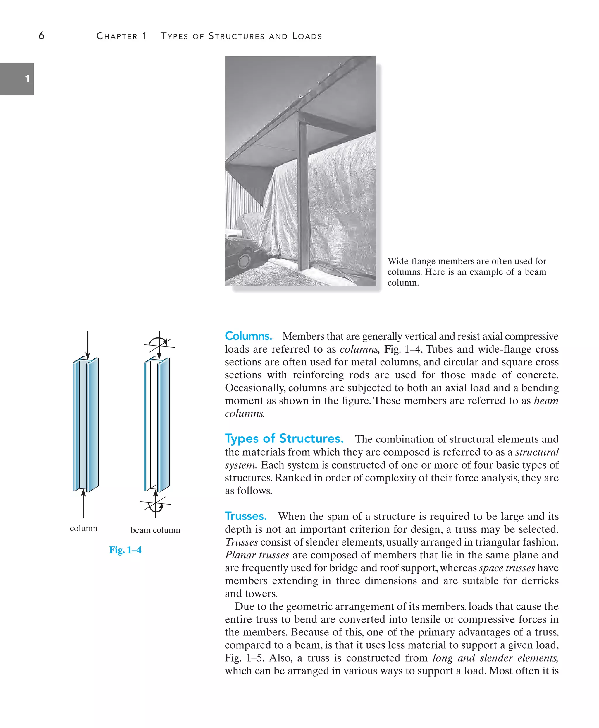
The girders of this bridge must resist the
maximum moment caused by the weight of
this jet plane as it passes over it.

6
MC
A
C
B
10 ft 30 ft
2 k 4 k 3 k
6 ft
4 ft
7.5
10 40
(a)
x
A
C
2 k 4 k 3 k
4 ft
10 ft 6 ft
B
Case 1
A
C
2 k 4 k 3 k
4 ft 6 ft
B
Case 3
(b)
A
C
2 k 4 k 3 k
4 ft
6 ft 6 ft
B
Case 2
4.5
7.5
6.0
6 10 16 40
MC
x
(c)
Fig. 6–29

6
Fig. 6–30
Determine the maximum positive shear created at point B in the beam
shown in Fig. 6–30a due to the wheel loads of the moving truck.
EXAMPLE 6.18
SOLUTION
The influence line for the shear at B is shown in Fig. 6–30b.
3-ft Movement of 4-k Load. Imagine that the 4-k load acts just to
the right of point B so that we obtain its maximum positive influence.
Since the beam segment BC is 10 ft long, the 10-k load is not as yet on
the beam. When the truck moves 3 ft to the left, the 4-k load jumps
downward on the influence line 1 unit and the 4-k, 9-k, and 15-k loads
create a positive increase in since the slope is upward to the left.
Although the 10-k load also moves forward 3 ft, it is still not on the
beam.Thus,
6-ft Movement of 9-k Load. When the 9-k load acts just to the right
of B, and then the truck moves 6 ft to the left, we have
Note in the calculation that the 10-k load only moves 4 ft on the beam.
¢VB = 91-12 + 14 + 9 + 152a
0.5
10
b162 + 10a
0.5
10
b142 = +1.4 k
¢VB = 41-12 + 14 + 9 + 152a
0.5
10
b3 = +0.2 k
¢VB,
6 ft
(a)
A
C
10 ft 10 ft 3 ft
6 ft
4 k 9 k 15 k 10 k
B
x
0.5
10 20
(b)
0.5
VB
influence line for VB

6
6-ft Movement of 15-k Load. If the 15-k load is positioned just to
the right of B and then the truck moves 6 ft to the left, the 4-k load
moves only 1 ft until it is off the beam, and likewise the 9-k load moves
only 4 ft until it is off the beam. Hence,
Since is now negative, the correct position of the loads
occurs when the 15-k load is just to the right of point B, Fig. 6–30c.
Consequently,
Ans.
In practice one also has to consider motion of the truck from left
to right and then choose the maximum value between these two
situations.
= 7.5 k
1VB2max = 41-0.052 + 91-0.22 + 1510.52 + 1010.22
¢VB
= -5.5 k
¢VB = 151-12 + 4a
0.5
10
b112 + 9a
0.5
10
b142 + 115 + 102a
0.5
10
b162
6 ft
A C
3 ft 6 ft
4 k 9 k 15 k 10 k
B
1 ft 4 ft
(c)
x
0.5
10 20
0.5
VB
1 4
0.05
0.2
16
0.2

6
Determine the maximum positive moment created at point B in the
beam shown in Fig. 6–31a due to the wheel loads of the crane.
EXAMPLE 6.19
SOLUTION
The influence line for the moment at B is shown in Fig. 6–31b.
2-m Movement of 3-kN Load. If the 3-kN load is assumed to act at
B and then moves 2 m to the right, Fig. 6–31b, the change in moment is
Why is the 4-kN load not included in the calculations?
3-m Movement of 8-kN Load. If the 8-kN load is assumed to act at
B and then moves 3 m to the right, the change in moment is
Notice here that the 4-kN load was initially 1 m off the beam, and
therefore moves only 2 m on the beam.
Since there is a sign change in the correct position of the
loads for maximum positive moment at B occurs when the 8-kN force
is at B, Fig. 6–31b.Therefore,
Ans.
1MB2max = 811.202 + 310.42 = 10.8 kN # m
¢MB,
= -8.40 kN # m
¢MB = -3a
1.20
3
b132 - 8a
1.20
3
b132 + 4a
1.20
2
b122
¢MB = -3a
1.20
3
b122 + 8a
1.20
3
b122 = 7.20 kN # m
2 m 3 m 2 m
A B C
4 kN
8 kN
3 kN
2 m
3 m
(a)
2 m 3 m
A B
4 kN
8 kN
3 kN
2 m
3 m
(b)
MB
1.20
2
5
0.8
x
0.4
7
Fig. 6–31

6
EXAMPLE 6.20
Determine the maximum compressive force developed in member
BG of the side truss in Fig. 6–32a due to the right side wheel loads of
the car and trailer. Assume the loads are applied directly to the truss
and move only to the right.
SOLUTION
The influence line for the force in member BG is shown in Fig. 6–32b.
Here a trial-and-error approach for the solution will be used. Since
we want the greatest negative (compressive) force in BG, we begin as
follows:
1.5-kN Load at Point C. In this case
4-kN Load at Point C. By inspection this would seem a more
reasonable case than the previous one.
2-kN Load at Point C. In this case all loads will create a compressive
force in BC.
Ans.
Since this final case results in the largest answer, the critical loading
occurs when the 2-kN load is at C.
= -2.66 kN
FBG = 2 kN1-0.6252 + 4 kNa
-0.625
6 m
b13 m2 + 1.5 kNa
-0.625
6 m
b11 m2
= -2.50 kN
FBG = 4 kN1-0.6252 + 1.5 kNa
-0.625
6 m
b14 m2 + 2 kN10.31252
= -0.729 kN
FBG = 1.5 kN1-0.6252 + 4102 + 2 kNa
0.3125
3 m
b11 m2
3
4 6 9 12
0.3125
0.625
FBG
x
(b)
influence line for FBG
A B C D E
3 m 3 m 3 m 3 m
4 m
(a)
1.5 kN
4 kN
2 kN
H G F
3 m 2 m
Fig. 6–32

6
6.7 Absolute Maximum Shear and Moment
In Sec. 6–6 we developed the methods for computing the maximum shear
and moment at a specified point in a beam due to a series of concentrated
moving loads. A more general problem involves the determination of
both the location of the point in the beam and the position of the loading
on the beam so that one can obtain the absolute maximum shear and
moment caused by the loads. If the beam is cantilevered or simply
supported, this problem can be readily solved.
Shear. For a cantilevered beam the absolute maximum shear will
occur at a point located just next to the fixed support. The maximum
shear is found by the method of sections, with the loads positioned
anywhere on the span, Fig. 6–33.
For simply supported beams the absolute maximum shear will occur just
next to one of the supports. For example, if the loads are equivalent, they
are positioned so that the first one in sequence is placed close to the
support, as in Fig. 6–34.
Moment. The absolute maximum moment for a cantilevered beam
occurs at the same point where absolute maximum shear occurs, although
in this case the concentrated loads should be positioned at the far end of
the beam, as in Fig. 6–35.
For a simply supported beam the critical position of the loads and the
associated absolute maximum moment cannot, in general, be determined
by inspection. We can, however, determine the position analytically. For
purposes of discussion, consider a beam subjected to the forces
shown in Fig. 6–36a. Since the moment diagram for a series of concen-
trated forces consists of straight line segments having peaks at each
force, the absolute maximum moment will occur under one of the forces.
Assume this maximum moment occurs under The position of the
loads on the beam will be specified by the distance x, measured
from to the beam’s centerline as shown.To determine a specific value
of x, we first obtain the resultant force of the system, and its distance
FR,
F2
F3
F2,
F1,
F2.
F3
F2,
F1,
Fig. 6–33
V
abs
max
V
abs
max
Mabs
max
F1
F2 F3
FR
By
Ay
A B
x
d2
d1
L
—
2
L
—
2
(a)
( x)
_
x¿
_
x¿
F1
d1
Ay
L
—
2
( x)
M2
V2
(b)
Fig. 6–34
Fig. 6–35
Fig. 6–36

6.7 ABSOLUTE MAXIMUM SHEAR AND MOMENT 251
6
measured from Once this is done, moments are summed about B,
which yields the beam’s left reaction, that is,
If the beam is sectioned just to the left of the resulting free-body
diagram is shown in Fig. 6–36b.The moment under is therefore
For maximum we require
or
Hence, we may conclude that the absolute maximum moment in a
simply supported beam occurs under one of the concentrated forces, such
that this force is positioned on the beam so that it and the resultant force
of the system are equidistant from the beam’s centerline. Since there are a
series of loads on the span (for example, in Fig. 6–36a), this
principle will have to be applied to each load in the series and the
corresponding maximum moment computed. By comparison, the largest
moment is the absolute maximum.As a general rule, though, the absolute
maximum moment often occurs under the largest force lying nearest the
resultant force of the system.
Envelope of Maximum Influence-Line Values. Rules or
formulations for determining the absolute maximum shear or moment
are difficult to establish for beams supported in ways other than the
cantilever or simple support discussed here. An elementary way to
proceed to solve this problem, however, requires constructing influence
lines for the shear or moment at selected points along the entire length
of the beam and then computing the maximum shear or moment in the
beam for each point using the methods of Sec. 6–6. These values when
plotted yield an “envelope of maximums,” from which both the absolute
maximum value of shear or moment and its location can be found.
Obviously, a computer solution for this problem is desirable for
complicated situations, since the work can be rather tedious if carried out
by hand calculations.
F3
F2,
F1,
x =
x¿
2
dM2
dx
=
-2FRx
L
+
FRx¿
L
= 0
M2
=
FRL
4
-
FRx¿
2
-
FRx2
L
+
FRxx¿
L
- F1d1
=
1
L
1FR2c
L
2
- 1x¿ - x2d a
L
2
- xb - F1d1
M2 = Aya
L
2
- xb - F1d1
©M = 0;
F2
M2
F2,
Ay =
1
L
1FR2c
L
2
- 1x¿ - x2d
©MB = 0;
Ay,
F2.
x¿
The absolute maximum moment in this
girder bridge is the result of the moving
concentrated loads caused by the wheels of
these train cars. The cars must be in the
critical position, and the location of the point
in the girder where the absolute maximum
moment occurs must be identified.

6
Determine the absolute maximum moment in the simply supported
bridge deck shown in Fig. 6–37a.
EXAMPLE 6.21
SOLUTION
The magnitude and position of the resultant force of the system are
determined first, Fig. 6–37a.We have
Let us first assume the absolute maximum moment occurs under
the 1.5-k load. The load and the resultant force are positioned
equidistant from the beam’s centerline, Fig. 6–37b. Calculating
first, Fig. 6–37b, we have
Now using the left section of the beam, Fig. 6–37c, yields
MS = 21.7 k # ft
-2.50116.672 + 21102 + MS = 0
d +©MS = 0;
-Ay1302 + 4.5116.672 = 0 Ay = 2.50 k
d +©MB = 0;
Ay
x = 6.67 ft
4.5x = 1.51102 + 11152
e +MRC
= ©MC;
FR = 2 + 1.5 + 1 = 4.5 k
+ TFR = ©F;
Ay 2.5 k
10 ft
MS
VS
1.5 k
2 k
6.67 ft
(c)
FR 4.5 k
A
B
15 ft
Ay By
(b)
15 ft
2 k 1.5 k 1 k
6.67 ft 6.67 ft
1.67 ft
5 ft
10 ft
1 k
2 k
FR 4.5 k
_
x6.67ft
30 ft
A
B
C
(a)
5 ft
1.5 k
Fig. 6–37

6
There is a possibility that the absolute maximum moment may
occur under the 2-k load, since and is between both 2 k
and 1.5 k. To investigate this case, the 2-k load and are positioned
equidistant from the beam’s centerline, Fig. 6–37d. Show that
as indicated in Fig. 6–37e and that
By comparison, the absolute maximum moment is
Ans.
which occurs under the 1.5-k load, when the loads are positioned on
the beam as shown in Fig. 6–37b.
MS = 21.7 k # ft
MS = 20.4 k # ft
Ay = 1.75 k
FR
FR
2 k 7 1.5 k
Ay 1.75 k
11.67 ft
MS
VS
2 k
(e)
FR 4.5 k
15 ft
Ay By
(d)
2 k 1.5 k
3.33 ft
11.67 ft
1 k

6
The truck has a mass of 2 Mg and a center of gravity at G as shown in
Fig. 6–38a. Determine the absolute maximum moment developed in
the simply supported bridge deck due to the truck’s weight.The bridge
has a length of 10 m.
SOLUTION
As noted in Fig. 6–38a, the weight of the truck,
and the wheel reactions have been calculated by statics.
Since the largest reaction occurs at the front wheel, we will select this
wheel along with the resultant force and position them equidistant from
the centerline of the bridge, Fig. 6–38b. Using the resultant force rather
than the wheel loads, the vertical reaction at B is then
The maximum moment occurs under the front wheel loading. Using
the right section of the bridge deck, Fig. 6–38c, we have
Ans.
Ms = 39.7 kN # m
8.82914.52 - Ms = 0
d +©Ms = 0;
By = 8.829 kN
By1102 - 19.6214.52 = 0
d +©MA = 0;
19.62kN,
21103
2kg19.81 m/s2
2 =
EXAMPLE 6.22
(a)
6.54 kN 13.08 kN
1 m
2 m
19.62 kN
G
5 m 5 m
(b)
A B
Ay By
6.54 kN
13.08 kN
13.08 kN
8.83 kN
0.5 m
0.5 m
19.62 kN
4.5 m
Vs
Ms
Fig. 6–38
(c)

6
6–59. Determine the maximum moment at point C on the
single girder caused by the moving dolly that has a mass of
2 Mg and a mass center at G.Assume A is a roller.
6–62. Determine the maximum positive moment at the
splice C on the side girder caused by the moving load which
travels along the center of the bridge.
PROBLEMS
*6–60. Determine the maximum moment in the
suspended rail at point B if the rail supports the load of
2.5 k on the trolley.
6–63. Determine the maximum moment at C caused by
the moving load.
*6–64. Draw the influence line for the force in member IH
of the bridge truss. Determine the maximum force (tension
or compression) that can be developed in this member
due to a 72-k truck having the wheel loads shown. Assume
the truck can travel in either direction along the center of the
deck, so that half its load is transferred to each of the two
side trusses.Also assume the members are pin connected at
the gusset plates.
G
5 m 5 m 5 m
C
B
A 1.5 m
0.5 m
Prob. 6–59
8 ft 8 ft
6 ft
6 ft
A B C
2.5 k
2 ft
1 ft
Prob. 6–61
8 ft 8 ft
6 ft
6 ft
A B C
2.5 k
2 ft
1 ft
Prob. 6–60
B
C
A
8 m 8 m 8 m
4 kN
4 m
8 kN
Prob. 6–62
15 ft 15 ft
A C B
2 ft 1 ft
2400 lb
Prob. 6–63
J I H G
A
B C D E
K L M
10 ft
10 ft
F
32 k 32 k
8 k
20 ft 20 ft 20 ft 20 ft 20 ft
25 ft 15 ft
Prob. 6–64
6–61. Determine the maximum positive shear at point B
if the rail supports the load of 2.5 k on the trolley.

6
6–65. Determine the maximum positive moment at
point C on the single girder caused by the moving load.
*6–68. Draw the influence line for the force in member IC
or compression) that can be developed in the member
the truck can travel in either direction along the center of
the deck, so that half the load shown is transferred to each
of the two side trusses. Also assume the members are pin
connected at the gusset plates.
6–66. The cart has a weight of 2500 lb and a center of
gravity at G. Determine the maximum positive moment
created in the side girder at C as it crosses the bridge.
Assume the car can travel in either direction along the
center of the deck, so that half its load is transferred to each
of the two side girders.
6–69. The truck has a mass of 4 Mg and mass center at
and the trailer has a mass of 1 Mg and mass center at
Determine the absolute maximum live moment developed
in the bridge.
G2.
G1,
6–67. Draw the influence line for the force in member BC
or compression) that can be developed in the member
the truck can travel in either direction along the center of the
deck, so that half the load shown is transferred to each of
the two side trusses. Also assume the members are pin
connected at the gusset plates.
6–70. Determine the absolute maximum live moment in
the bridge in Problem 6–69 if the trailer is removed.
5 m
A B
2 m
1.5 m
4 kN 6 kN 8 kN
5 m
C
Prob. 6–65
8 ft 8 ft
A B
1.5 ft 1 ft
G
C
Prob. 6–66
J I H G
D
C
B
E
F
15 ft
2 k
3 k
8 ft
A
20 ft 20 ft 20 ft 20 ft
Probs. 6–67/6–68
8 m
A B
G1
G2
1.5 m
0.75 m
1.5 m
Prob. 6–69
8 m
A B
G1
G2
1.5 m
0.75 m
1.5 m
Prob. 6–70

6
6–71. Determine the absolute maximum live shear
and absolute maximum moment in the jib beam AB
due to the 10-kN loading. The end constraints require
0.1 m … x … 3.9 m.
6–73. Determine the absolute maximum moment in the
girder bridge due to the truck loading shown. The load is
applied directly to the girder.
*6–72. Determine the maximum moment at C caused by
the moving loads.
6–74. Determine the absolute maximum shear in the beam
due to the loading shown.
4 m
x
A B
10 kN
Prob. 6–71
20 ft 30 ft
C
A B
2 k
2 k
4 k
6 k
3 ft 4 ft 3 ft
Prob. 6–72
B
80 ft
20 ft
8 ft
10 k
15 k
7 k
3 k
4 ft
A
Prob. 6–73
12 m
20 kN
25 kN
40 kN
4 m
A B
1.5 m
Prob. 6–75
12 m
20 kN
25 kN
40 kN
4 m
A B
1.5 m
Prob. 6–74
beam due to the loading shown.

6
*6–76. Determine the absolute maximum shear in the
bridge girder due to the loading shown.
6–79. Determine the absolute maximum shear in the beam
due to the loading shown.
girder due to the loading shown.
6–81. The trolley rolls at C and D along the bottom and
top flange of beam AB. Determine the absolute maximum
moment developed in the beam if the load supported by the
trolley is 2 k. Assume the support at A is a pin and at B a
roller.
30 ft
8 ft
B
A
10 k
6 k
Prob. 6–77
30 ft
8 ft
B
A
10 k
6 k
Prob. 6–76
25 ft
10 k
8 k
3 k
2 ft
2 ft
3 ft
4 k
Prob. 6–78
30 ft
3 k
6 k
2 k
3 ft
3 ft
5 ft
4 k
Prob. 6–80
30 ft
3 k
6 k
2 k
3 ft
3 ft
5 ft
4 k
Prob. 6–79
A
D
B
C
1 ft
0.5 ft
20 ft
Prob. 6–81
bridge girder due to the loading shown.
*6–80. Determine the absolute maximum moment in the
bridge due to the loading shown.

6
6–1P. The chain hoist on the wall crane can be placed
anywhere along the boom and has a
rated capacity of 28 kN. Use an impact factor of 0.3 and
determine the absolute maximum bending moment in the
boom and the maximum force developed in the tie rod BC.
The boom is pinned to the wall column at its left end A.
Neglect the size of the trolley at D.
(0.1 m 6 x 6 3.4 m)
6–2P. A simply supported pedestrian bridge is to be
constructed in a city park and two designs have been
proposed as shown in case a and case b. The truss members
are to be made from timber.The deck consists of 1.5-m-long
planks that have a mass of .A local code states the
live load on the deck is required to be 5 kPa with an impact
factor of 0.2. Consider the deck to be simply supported on
stringers. Floor beams then transmit the load to the bottom
joints of the truss. (See Fig. 6–23.) In each case find the
member subjected to the largest tension and largest
compression load and suggest why you would choose one
design over the other. Neglect the weights of the truss
members.
20 kgm2
PROJECT PROBLEMS
0.75 m
3 m
x
0.5 m
0.1 m
28 kN
A
D
B
C
Prob. 6–1P
E
1.25 m 1.25 m 1.25 m 1.25 m
1.25 m
case b
A
B C D
F
G
H
1.25 m 1.25 m 1.25 m 1.25 m
1.25 m
case a
A
B C D
E
E
F
G
H
Prob. 6–2P

6
An influence line indicates the value of a reaction, shear, or moment at a specific point on a member, as a unit load moves
over the member.
Once the influence line for a reaction, shear, or moment (function) is constructed, then it will be possible to locate the
live load on the member to produce the maximum positive or negative value of the function.
A concentrated live force is applied at the positive (negative) peaks of the influence line. The value of the function is
then equal to the product of the influence line ordinate and the magnitude of the force.
The general shape of the influence line can be established using the Müller-Breslau principle, which states that the
influence line for a reaction, shear, or moment is to the same scale as the deflected shape of the member when it is acted
upon by the reaction, shear, or moment.
1
1
––
2
Ay
1
––
2
L
1
––
2 )F
Ay (
L
x
B
A
L
F
1
x __ L
2
Ay
A B
L
Ay
w0 Ay
1
L
x
1
––
2
(1)(L)(w0)
Ay
Ay
deflected shape
(b)
A uniform distributed load extends over a positive (negative) region of the influence line. The value of the function is
then equal to the product of the area under the influence line for the region and the magnitude of the uniform load.
A
(a)
CHAPTER REVIEW

CHAPTER REVIEW 261
6
Influence lines for floor girders and trusses can be established by placing the unit load at each panel point or joint, and
calculating the value of the required reaction, shear, or moment.
When a series of concentrated loads pass over the member, then the various positions of the load on the member have
to be considered to determine the largest shear or moment in the member. In general, place the loadings so that each
contributes its maximum influence, as determined by multiplying each load by the ordinate of the influence line. This
process of finding the actual position can be done using a trial-and-error procedure, or by finding the change in either the
shear or moment when the loads are moved from one position to another. Each moment is investigated until a negative
value of shear or moment occurs. Once this happens the previous position will define the critical loading.
V
abs
max
Absolute maximum moment in a cantilevered beam
occurs when the series of concentrated loads are placed
at the farthest point away from the fixed support.
F1
F2 F3
FR
By
Ay
L
—
2
—
2
L
—
2
_
x¿
_
x¿ —
2
_
x¿
Absolute maximum shear in a cantilever or simply
supported beam will occur at a support, when one of the
loads is placed next to the support.
To determine the absolute maximum moment in a simply
supported beam, the resultant of the force system is first
determined. Then it, along with one of the concentrated
forces in the system is positioned so that these two forces
are equidistant from the centerline of the beam. The
maximum moment then occurs under the selected force.
Each force in the system is selected in this manner, and
by comparison the largest for all these cases is the
absolute maximum moment.
Mabs
max
V
abs
max

The portal to this bridge must resist loteral loads due to wind and traffic. An
approximate analysis can be made of the forces produced for a preliminary
design of the members, before a more exact structural analysis is done.

7
263
In this chapter we will present some of the approximate methods used
to analyze statically indeterminate trusses and frames. These methods
were developed on the basis of structural behavior, and their accuracy
in most cases compares favorably with more exact methods of analysis.
Although not all types of structural forms will be discussed here, it is
hoped that enough insight is gained from the study of these methods
so that one can judge what would be the best approximations to
make when performing an approximate force analysis of a statically
indeterminate structure.
7.1 Use of Approximate Methods
When a model is used to represent any structure, the analysis of it must
satisfy both the conditions of equilibrium and compatibility of
displacement at the joints.As will be shown in later chapters of this text,
the compatibility conditions for a statically indeterminate structure can
be related to the loads provided we know the material’s modulus of
elasticity and the size and shape of the members. For an initial design,
however, we will not know a member’s size, and so a statically
indeterminate analysis cannot be considered. For analysis a simpler model
of the structure must be developed, one that is statically determinate.
Once this model is specified, the analysis of it is called an approximate
analysis. By performing an approximate analysis, a preliminary design of
the members of a structure can be made, and when this is complete, the
more exact indeterminate analysis can then be performed and the design
refined. An approximate analysis also provides insight as to a structure’s
behavior under load and is beneficial when checking a more exact analysis
or when time, money, or capability are not available for performing the
more exact analysis.
Approximate Analysis of
Statically Indeterminate
Structures

264 CHAPTER 7 APPROXIMATE ANALYSIS OF STATICALLY INDETERMINATE STRUCTURES
Realize that, in a general sense, all methods of structural analysis are
approximate, simply because the actual conditions of loading, geometry,
material behavior, and joint resistance at the supports are never known in
an exact sense.In this text,however,the statically indeterminate analysis of
a structure will be referred to as an exact analysis, and the simpler statically
determinate analysis will be referred to as the approximate analysis.
7.2 Trusses
A common type of truss often used for lateral bracing of a building or
for the top and bottom cords of a bridge is shown in Fig. 7–1a. (Also see
Fig. 3–4.) When used for this purpose, this truss is not considered a
primary element for the support of the structure, and as a result it is
often analyzed by approximate methods. In the case shown, it will be
noticed that if a diagonal is removed from each of the three panels, it
will render the truss statically determinate. Hence, the truss is statically
indeterminate to the third degree (using Eq. 3–1, or
) and therefore we must make three assumptions
regarding the bar forces in order to reduce the truss to one that is
statically determinate. These assumptions can be made with regard to
the cross-diagonals, realizing that when one diagonal in a panel is in
tension the corresponding cross-diagonal will be in compression. This is
evident from Fig. 7–1b, where the “panel shear” V is carried by the
vertical component of tensile force in member a and the vertical
component of compressive force in member b. Two methods of analysis
are generally acceptable.
Method 1: If the diagonals are intentionally designed to be long
and slender, it is reasonable to assume that they cannot
support a compressive force; otherwise, they may easily
buckle. Hence the panel shear is resisted entirely by the
tension diagonal, whereas the compressive diagonal is
assumed to be a zero-force member.
Method 2: If the diagonal members are intended to be constructed
from large rolled sections such as angles or channels, they
may be equally capable of supporting a tensile and
compressiveforce.Herewewillassumethatthetensionand
compression diagonals each carry half the panel shear.
Both of these methods of approximate analysis are illustrated
numerically in the following examples.
16 + 3 7 8122
b + r 7 2j,
7
a
b
P2
P1
(a)
R1 R2
F2
F1
R1
Fb
Fa
V R1
(b)
Fig. 7–1
An approximate method can be used to determine the
forces in the cross bracing in each panel of this bascule
railroad bridge. Here the cross members are thin and
so we can assume they carry no compressive force.

7.2 TRUSSES 265
7
EXAMPLE 7.1
Determine (approximately) the forces in the members of the truss
shown in Fig. 7–2a. The diagonals are to be designed to support both
tensile and compressive forces, and therefore each is assumed to carry
half the panel shear.The support reactions have been computed.
FEB
E
6.67 kN
8.33 kN
5 3
4
(f)
6.67 kN
5
4
3
8.33 kN
FAF
A
10 kN
6.67 kN
8.33 kN
5
4
3
(c)
D
C
3 m
10 kN
FED
FDB
FEC
FBC
V 10 kN 3
4
5
(d)
4
5
3
FDC
D
6.67 kN
8.33 kN
5 3
4
(e)
10 kN 10 kN
20 kN
(a)
A
4 m 4 m
3 m
B
C
D
E
20 kN
F
F
A
3 m
10 kN
20 kN
FFE
FFB F
FAE F
FAB
V 10 kN
3
4
5
(b)
3
4
5
Fig. 7–2
SOLUTION
By inspection the truss is statically indeterminate to the second
degree. The two assumptions require the tensile and compressive
diagonals to carry equal forces, that is, For a vertical
section through the left panel, Fig. 7–2b, we have
Ans.
so that
Ans.
Ans.
Ans.
Ans.
From joint A, Fig. 7–2c,
Ans.
A vertical section through the right panel is shown in Fig. 7–2d.
Show that
Ans.
Ans.
Furthermore, using the free-body diagrams of joints D and E,
Figs. 7–2e and 7–2f, show that
Ans.
Ans.
FEB = 10 kN 1T2
FDC = 5 kN 1C2
FEC = 8.33 kN 1C2, FBC = 6.67 kN 1T2
FDB = 8.33 kN 1T2, FED = 6.67 kN 1C2
+ c ©Fy = 0; FAF - 8.33A3
5 B - 10 = 0 FAF = 15 kN 1T2
d+©MF = 0; -8.33A4
5 B132 + FAB132 = 0 FAB = 6.67 kN 1T2
d+©MA = 0; -8.33A4
5 B132 + FFE132 = 0 FFE = 6.67 kN 1C2
FAE = 8.33 kN 1C2
FFB = 8.33 kN 1T2
+ c©Fy = 0; 20 - 10 - 2A3
5 BF = 0 F = 8.33 kN
FFB = FAE = F.

7
Cross bracing is used to provide lateral support for this bridge deck due
to the wind and unbalanced traffic loads. Determine (approximately)
the forces in the members of this truss. Assume the diagonals are
slender and therefore will not support a compressive force. The loads
and support reactions are shown in Fig. 7–3a.
EXAMPLE 7.2
(a)
8 k
A
8 k
15 ft 15 ft 15 ft 15 ft
B C D E
2 k
15 ft
F
4 k
G
4 k
H
4 k
I
2 k
J
8 k
A
2 k
J
V 6 k
FAI 0
FAB
FJB
FJI
15 ft
(b)
45
45
A
8 k
0
0
FJA
(c)
Fig. 7–3
SOLUTION
By inspection the truss is statically indeterminate to the fourth
degree. Thus the four assumptions to be used require that each
compression diagonal sustain zero force. Hence, from a vertical
section through the left panel, Fig. 7–3b, we have
Ans.
Ans.
Ans.
Ans.
From joint A, Fig. 7–3c,
Ans.
FJA = 8 k 1C2
FAB = 0
-FAB1152 = 0
d+©MJ = 0;
FJI = 6 k 1C2
-8.49 sin 45°1152 + FJI1152 = 0
d+©MA = 0;
FJB = 8.49 k 1T2
8 - 2 - FJB cos 45° = 0
+ c©Fy = 0;
FAI = 0

7.2 TRUSSES 267
7
A vertical section of the truss through members IH, IC, BH, and BC
is shown in Fig. 7–3d.The panel shear is
We require
Ans.
Ans.
Ans.
Ans.
From joint B, Fig. 7–3e,
Ans.
The forces in the other members can be determined by symmetry,
except however, from joint C, Fig. 7–3f, we have
Ans.
FCH = 4 k 1C2
212.83 sin 45°2 - FCH = 0
+ c ©Fy = 0;
FCH;
FBI = 6 k 1C2
8.49 sin 45° - FBI = 0
+ c ©Fy = 0;
FBC = 6 k 1T2
-81152 + 21152 + FBC1152 = 0
d+©MI = 0;
FIH = 8 k 1C2
-81152 + 21152 - 2.83 sin 45°1152 + FIH1152 = 0
d+©MB = 0;
FIC = 2.83 k 1T2
8 - 2 - 4 - FIC cos 45° = 0
+ c©Fy = 0;
FBH = 0
V = ©Fy = 8 - 2 - 4 = 2 k.
8 k
A
15 ft
B
4 k
I
2 k
J
V 2 k
FIH
FIC
FBH 0
FBC
15 ft
45
45
(d)
FBI
8.49 k
6 k
0
0
45
45
45
B
(e)
FCH
2.83 k
6 k
2.83 k
6 k
45
45
C
(f)

7
7–1. Determine (approximately) the force in each member
of the truss. Assume the diagonals can support either a
tensile or a compressive force.
7–2. Solve Prob. 7–1 assuming that the diagonals cannot
support a compressive force.
7–6. Solve Prob. 7–5 assuming that the diagonals cannot
PROBLEMS
*7–4. Solve Prob. 7–3 assuming that the diagonals cannot
tensile or compressive force.
*7–8. Solve Prob. 7–7 assuming that the diagonals cannot
Probs. 7–5/7–6
Probs. 7–3/7–4
Probs. 7–1/7–2
3 m
3 m
3 m
50 kN
A
D
B
C
40 kN 20 kN
F E
20 ft
20 ft
20 ft 20 ft
10 k
H
A D
B C
10 k
G
10 k
F
10 k
5 k
E
8 ft
6 ft
8 ft 8 ft
7 k
H
A D
B C
14 k
G
14 k
F
7 k
2 k
E
8 kN
4 kN
F E D
1.5 m
A B C
2 m 2 m
Probs. 7–7/7–8

7.2 TRUSSES 269
7
of the truss. Assume the diagonals can support both tensile
and compressive forces.
7–11. Determine (approximately) the force in each
member of the truss. Assume the diagonals can support
either a tensile or compressive force.
15 ft
15 ft
2 k
2 k
1.5 k
15 ft
15 ft
E
F
A B
C
G
D
8 kN
1.5 m
E
F
A
B
C
D
10 kN
2 m
2 m
Prob. 7–12
Prob. 7–10
15 ft
15 ft
2 k
2 k
1.5 k
15 ft
15 ft
E
F
A B
C
G
D
8 kN
1.5 m
E
F
A
B
C
D
10 kN
2 m
2 m
Prob. 7–11
Prob. 7–9
of the truss. Assume the diagonals DG and AC cannot
*7–12. Determine (approximately) the force in each
member of the truss. Assume the diagonals cannot support
a compressive force.

7.3 Vertical Loads on Building Frames
Building frames often consist of girders that are rigidly connected to
columns so that the entire structure is better able to resist the effects of
lateral forces due to wind and earthquake. An example of such a rigid
framework, often called a building bent, is shown in Fig. 7–4.
In practice, a structural engineer can use several techniques for
performing an approximate analysis of a building bent. Each is based
upon knowing how the structure will deform under load. One technique
would be to consider only the members within a localized region of the
structure.This is possible provided the deflections of the members within
the region cause little disturbance to the members outside the region.
Most often, however, the deflection curve of the entire structure is
considered. From this, the approximate location of points of inflection,
that is,the points where the member changes its curvature,can be specified.
These points can be considered as pins since there is zero moment within
the member at the points of inflection. We will use this idea in this
section to analyze the forces on building frames due to vertical loads, and
in Secs. 7–5 and 7–6 an approximate analysis for frames subjected to
lateral loads will be presented. Since the frame can be subjected to both
of these loadings simultaneously, then, provided the material remains
elastic, the resultant loading is determined by superposition.
Assumptions for Approximate Analysis. Consider a typical
girder located within a building bent and subjected to a uniform vertical
load, as shown in Fig. 7–5a. The column supports at A and B will each
exert three reactions on the girder, and therefore the girder will be
statically indeterminate to the third degree (6 reactions – 3 equations of
equilibrium). To make the girder statically determinate, an approximate
analysis will therefore require three assumptions. If the columns are
extremely stiff, no rotation at A and B will occur, and the deflection
7
typical building frame
Fig. 7–4

7.3 VERTICAL LOADS ON BUILDING FRAMES 271
curve for the girder will look like that shown in Fig. 7–5b. Using one of
the methods presented in Chapters 9 through 11, an exact analysis
reveals that for this case inflection points, or points of zero moment,
occur at 0.21L from each support. If, however, the column connections at
A and B are very flexible, then like a simply supported beam, zero
moment will occur at the supports, Fig. 7–5c. In reality, however, the
columns will provide some flexibility at the supports, and therefore we
will assume that zero moment occurs at the average point between the
two extremes, i.e., at from each support, Fig. 7–5d.
Furthermore, an exact analysis of frames supporting vertical loads
indicates that the axial forces in the girder are negligible.
In summary then, each girder of length L may be modeled by a simply
supported span of length 0.8L resting on two cantilevered ends, each
having a length of 0.1L, Fig. 7–5e. The following three assumptions are
incorporated in this model:
1. There is zero moment in the girder, 0.1L from the left support.
2. There is zero moment in the girder, 0.1L from the right support.
3. The girder does not support an axial force.
By using statics, the internal loadings in the girders can now be
obtained and a preliminary design of their cross sections can be made.
The following example illustrates this numerically.
10.21L + 022 L 0.1L
7
w column
column
girder
A B
L
(a)
w
A B
L
points of zero
moment
0.21L 0.21L
fixed supported
(b)
w
A B
L
simply supported
(c)
point of
zero
moment
point of
zero
moment
w
L
assumed points of zero
moment
0.1L
approximate case
(d)
0.1L
Fig. 7–5
w
0.1L
model
(e)
0.1L
0.8L

7
Fig. 7–6
Determine (approximately) the moment at the joints E and C caused
by members EF and CD of the building bent in Fig. 7–6a.
EXAMPLE 7.3
SOLUTION
For an approximate analysis the frame is modeled as shown in Fig. 7–6b.
Note that the cantilevered spans supporting the center portion of the
girder have a length of Equilibrium requires the
end reactions for the center portion of the girder to be 6400 lb, Fig. 7–6c.
The cantilevered spans are then subjected to a reaction moment of
Ans.
This approximate moment, with opposite direction, acts on the joints
at E and C, Fig. 7–6a. Using the results, the approximate moment
diagram for one of the girders is shown in Fig. 7–6d.
M = 1600112 + 6400122 = 14 400 lb # ft = 14.4 k # ft
0.1L = 0.11202 = 2 ft.
800 lb/ft
E F
C D
A B
800 lb/ft
20 ft
(a)
800 lb/ft
16 ft
800 lb/ft
2 ft 2 ft
(b)
16 ft
6400 lb 6400 lb
12 800 lb
1600 lb 6400 lb
14 400 lbft 14 400 lbft
1600 lb
6400 lb
8000 lb 8000 lb
2 ft 2 ft
(c)
M (kft)
x (ft)
20
18
2
14.4
25.6
(d)

7.4 PORTAL FRAMES AND TRUSSES 273
7.4 Portal Frames and Trusses
Frames. Portal frames are frequently used over the entrance of a
bridge*
and as a main stiffening element in building design in order to
transfer horizontal forces applied at the top of the frame to the
foundation. On bridges, these frames resist the forces caused by wind,
earthquake, and unbalanced traffic loading on the bridge deck. Portals
can be pin supported, fixed supported, or supported by partial fixity.The
approximate analysis of each case will now be discussed for a simple
three-member portal.
Pin Supported. A typical pin-supported portal frame is shown in
Fig. 7–7a. Since four unknowns exist at the supports but only three
equilibrium equations are available for solution, this structure is statically
indeterminate to the first degree. Consequently, only one assumption
must be made to reduce the frame to one that is statically determinate.
The elastic deflection of the portal is shown in Fig. 7–7b. This diagram
indicates that a point of inflection, that is, where the moment changes
from positive bending to negative bending, is located approximately at
the girder’s midpoint. Since the moment in the girder is zero at this point,
we can assume a hinge exists there and then proceed to determine the
reactions at the supports using statics. If this is done, it is found that the
horizontal reactions (shear) at the base of each column are equal and
the other reactions are those indicated in Fig. 7–7c. Furthermore, the
moment diagrams for this frame are indicated in Fig. 7–7d.
7
l
h
P
(a)
2
Ph
—
2
Ph
—
2
Ph
—
2
Ph
—
moment
diagram
(d)
l
h
P

assumed
hinge
(b)
l
—
2
P
—
2
P
—
l
Ph
—
2
l
Ph
—
h
2
P
—
l
Ph
—
2
P
—
l
Ph
—
h
P
(c)
l
—
2
*See Fig. 3–4.
Fig. 7–7

Fixed Supported. Portals with two fixed supports, Fig. 7–8a, are
statically indeterminate to the third degree since there are a total of six
unknowns at the supports. If the vertical members have equal lengths
and cross-sectional areas, the frame will deflect as shown in Fig. 7–8b. For
this case we will assume points of inflection occur at the midpoints of all
three members, and therefore hinges are placed at these points. The
reactions and moment diagrams for each member can therefore be
determined by dismembering the frame at the hinges and applying
the equations of equilibrium to each of the four parts. The results are
shown in Fig. 7–8c. Note that, as in the case of the pin-connected portal,
the horizontal reactions (shear) at the base of each column are equal.
The moment diagram for this frame is indicated in Fig. 7–8d.
7
Partial Fixity. Since it is both difficult and costly to construct a
perfectly fixed support or foundation for a portal frame, it is conservative
and somewhat realistic to assume a slight rotation occurs at the supports,
Fig. 7–9a. As a result, the points of inflection on the columns lie
somewhere between the case of having a pin-supported portal, Fig. 7–7a,
where the “inflection points” are at the supports (base of columns), and a
fixed-supported portal, Fig. 7–8a, where the inflection points are at the
center of the columns. Many engineers arbitrarily define the location at
, Fig. 7–9b, and therefore place hinges at these points, and also at the
center of the girder.
h3
h
P
(b)

assumed
hinges
l
h
P
(a)
P
2
h
—
2l
Ph
—
2
P
—
2
l
—
2
P
—
2l
Ph
—
2
P
—
2l
Ph
—
2
P
—
2l
Ph
—
2l
Ph
— 2l
Ph
—
2
P
—
4
Ph
—
2
P
—
2l
Ph
—
4
Ph
—
2
P
—
2l
Ph
—
2
h
—
(c)
2
P
—
4
Ph
—
(d)
moment
diagram
4
Ph
—
4
Ph
—
4
Ph
—
4
Ph
—
4
Ph
—
Fig. 7–8

Trusses. When a portal is used to span large distances, a truss may be
used in place of the horizontal girder. Such a structure is used on large
bridges and as transverse bents for large auditoriums and mill buildings.
A typical example is shown in Fig. 7–10a. In all cases, the suspended truss
is assumed to be pin connected at its points of attachment to the columns.
Furthermore, the truss keeps the columns straight within the region of
attachment when the portal is subjected to the sidesway Fig. 7–10b.
Consequently, we can analyze trussed portals using the same assumptions
as those used for simple portal frames. For pin-supported columns,
assume the horizontal reactions (shear) are equal, as in Fig. 7–7c. For
fixed-supported columns, assume the horizontal reactions are equal and
an inflection point (or hinge) occurs on each column, measured midway
between the base of the column and the lowest point of truss member
connection to the column. See Fig. 7–8c and Fig. 7–10b.
The following example illustrates how to determine the forces in the
members of a trussed portal using the approximate method of analysis
described above.
¢,
7
l
h
P
(a)
P
(b)
assumed
hinges
3
h
—
3
h
—
u u
P
h
l
(a)
P
(b)
h
—
2

P
—
2
P
—
2
assumed
hinges
Fig. 7–10
Fig. 7–9

7
Determine by approximate methods the forces acting in the members
of the Warren portal shown in Fig. 7–11a.
EXAMPLE 7.4
SOLUTION
The truss portion B, C, F, G acts as a rigid unit. Since the supports
are fixed, a point of inflection is assumed to exist
above A and I, and equal horizontal reactions or shear act at the base
of the columns, i.e., With these
assumptions, we can separate the structure at the hinges J and K,
Fig. 7–11b, and determine the reactions on the columns as follows:
Lower Half of Column
Upper Portion of Column
d+©MJ = 0; -4015.52 + N182 = 0 N = 27.5 kN
d+©MA = 0; M - 3.51202 = 0 M = 70 kN # m
V = 40 kN2 = 20 kN.
©Fx = 0;
7 m2 = 3.5 m
(a)
8 m
4 m 2 m
2 m
2 m
7 m
4 m
C D E
B H
F
G
A
I
40 kN
3.5 m
40 kN
V 20 kN
N
V 20 kN
J
A
K
N
M
N
V 20 kN
V 20 kN
N
N
V 20 kN
3.5 m
M
N
V 20 kN
5.5 m
(b)
Fig. 7–11

7
Using the method of sections, Fig. 7–11c, we can now proceed to
obtain the forces in members CD, BD, and BH.
Ans.
Ans.
Ans.
In a similar manner, show that one obtains the results on the free-
body diagram of column FGI in Fig. 7–11d. Using these results, we can
now find the force in each of the other truss members of the portal
using the method of joints.
Joint D, Fig. 7–11e
Ans.
Ans.
Joint H, Fig. 7–11f
Ans.
These results are summarized in Fig. 7–11g.
FHE sin 45° - 38.9 sin 45° = 0 FHE = 38.9 kN 1T2
+ c©Fy = 0;
75 - 2138.9 cos 45°2 - FDE = 0 FDE = 20 kN 1C2
:
+ ©Fx = 0;
FDH sin 45° - 38.9 sin 45° = 0 FDH = 38.9 kN 1C2
+ c©Fy = 0;
FBH = 27.5 kN 1T2
FBH122 - 2015.52 + 27.5122 = 0
d+©MD = 0;
FCD = 75 kN 1C2
-2013.52 - 40122 + FCD122 = 0
d+©MB = 0;
FBD = 38.9 kN 1T2
-27.5 + FBD sin 45° = 0
+ c©Fy = 0;
40 kN
20 kN
2 m
3.5 m
27.5 kN
2 m
FCD
FBD
FBH
45
B
(c)
D
20 kN
2 m
3.5 m
27.5 kN
2 m
45
G
35 kN
E
38.9 kN
27.5 kN
(d)
FDE
FDH
45 45
75 kN
38.9 kN
y
x
D
(e)
FHE
45 45
27.5 kN
y
x
H
38.9 kN
27.5 kN
(f)
40 kN
20 kN
70 kNm
27.5 kN 27.5 kN
70 kNm
20 kN
C D E F
B
H
G
75 kN(C) 20 kN(C) 35 kN(T)
27.5 kN (T)
3
8
.
9
k
N
(
T
)
27.5 kN (C)
38.9 kN
(C) 38.9 kN
(T)
(g)
3
8
.
9
k
N
(
C
)

7
Prob. 7–13
6 m
A B C D
E F G H
8 m 6 m
6 m
3 kN/m
Prob. 7–14
400 lb/ft
F
E
A B C
D
15 ft 20 ft
Prob. 7–15
8 m
A
C
E
B
D
F
5 kN/m
9 kN/m
Prob. 7–16
A B D
E
F
K
L
G
H I J
C
5 kN/m
5 kN/m
3 kN/m
8 m 8 m 8 m
7–13. Determine (approximately) the internal moments
at joints A and B of the frame.
7–15. Determine (approximately) the internal moment at
A caused by the vertical loading.
PROBLEMS
at joints F and D of the frame.
*7–16. Determine (approximately) the internal moments
at A and B caused by the vertical loading.

7
Prob. 7–17
20 ft 40 ft 30 ft
A
H
I
B
G F
K
L
E
D
J
C
0.5 k/ft
1.5 k/ft 1.5 k/ft
Prob. 7–18
15 ft 20 ft
A
D
F
C
H
G
E
B
400 lb/ft
1200 lb/ft
7–18. Determine (approximately) the support actions at
A, B, and C of the frame.
*7–20. Determine (approximately) the internal moment
and shear at the ends of each member of the portal frame.
Assume the supports at A and D are partially fixed, such
that an inflection point is located at h/3 from the bottom of
each column.
at joints I and L. Also, what is the internal moment at joint
H caused by member HG?
7–19. Determine (approximately) the support reactions
at A and B of the portal frame. Assume the supports are
(a) pinned, and (b) fixed.
Prob. 7–19
6 m
4 m
12 kN
A
D C
B
Prob. 7–20
P
B
A
C
D
b
h

7
Probs. 7–21/7–22
7 ft
500 lb
B
A
E G
H
F
D
C
6 ft
1.5 ft
1.5 ft 1.5 ft
Probs. 7–23/7–24
8 ft
2 k
8 ft
6 ft
12 ft
A B
C D
F
E
G
1 k
Prob. 7–25
2 m 2 m
1.5 m
5 m
A B
D
G
F
C
E
4 kN
8 kN
Prob. 7–26
2 m 2 m
1.5 m
5 m
A B
D
G
F
C
E
4 kN
8 kN
7–21. Draw (approximately) the moment diagram for
member ACE of the portal constructed with a rigid member
EG and knee braces CF and DH. Assume that all points of
connection are pins. Also determine the force in the knee
brace CF.
7–22. Solve Prob. 7–21 if the supports at A and B are fixed
instead of pinned.
7–25. Draw (approximately) the moment diagram for col-
umn AGF of the portal. Assume all truss members and the
columns to be pin connected at their ends. Also determine
the force in all the truss members.
7–23. Determine (approximately) the force in each truss
member of the portal frame. Also find the reactions at the
fixed column supports A and B.Assume all members of the
truss to be pin connected at their ends.
*7–24. Solve Prob. 7–23 if the supports at A and B are
pinned instead of fixed.
7–26. Draw (approximately) the moment diagram for col-
umn AGF of the portal. Assume all the members of the
truss to be pin connected at their ends. The columns are
fixed at A and B. Also determine the force in all the truss
members.

7
7–27. Determine (approximately) the force in each truss
member of the portal frame. Also find the reactions at the
fixed column supports A and B.Assume all members of the
truss to be pin connected at their ends.
pinned instead of fixed.
column ACD of the portal. Assume all truss members and
the columns to be pin connected at their ends. Also
determine the force in members FG, FH, and EH.
fixed instead of pinned.
7–29. Determine (approximately) the force in members
GF, GK, and JK of the portal frame.Also find the reactions
at the fixed column supports A and B.Assume all members
of the truss to be connected at their ends.
7–30. Solve Prob. 7–29 if the supports at A and B are pin
connected instead of fixed.
column AJI of the portal.Assume all truss members and the
columns to be pin connected at their ends. Also determine
the force in members HG, HL, and KL.
7–34. Solve Prob. 7–33 if the supports at A and B are fixed
instead of pinned.
6 m
6 m
1.5 m
1.5 m
3 m
3 m
8 kN
8 kN
A
A
F
F
I
I
G
G
B
B
2 m
2 m
1.5 m
1.5 m
H
H C
C
D
D
E
E
3 m
3 m 3 m
3 m
12 kN
12 kN
Probs. 7–27/7–28
D
C
E
H
I
K
F
L
J
G
8 ft 8 ft 8 ft 8 ft
12 ft
3 ft
6 ft
A
4 k
B
Probs. 7–29/7–30
D
C
E H I
K
F
L
J
G
8 ft 8 ft 8 ft 8 ft
12 ft
3 ft
6 ft
6 ft
A
4 k
B
Probs. 7–31/7–32
4 kN
2 kN
O
K L M N
A B
C
D
E
F
G
J
I
H
1.5 m
4 m
1 m
6 @ 1.5 m 9 m
Probs. 7–33/7–34

7
Portal Method
In Sec. 7–4 we discussed the action of lateral loads on portal frames and
found that for a frame fixed supported at its base, points of inflection
occur at approximately the center of each girder and column and the
columns carry equal shear loads, Fig. 7–8. A building bent deflects in
the same way as a portal frame, Fig. 7–12a, and therefore it would be
appropriate to assume inflection points occur at the center of the columns
and girders. If we consider each bent of the frame to be composed of a
series of portals, Fig. 7–12b, then as a further assumption, the interior
columns would represent the effect of two portal columns and would
therefore carry twice the shear V as the two exterior columns.
(a)
P
inflection point
(b)
V V V V
Fig. 7–12

7.5 LATERAL LOADS ON BUILDING FRAMES: PORTAL METHOD 283
7
In summary, the portal method for analyzing fixed-supported building
frames requires the following assumptions:
1. A hinge is placed at the center of each girder, since this is assumed
to be a point of zero moment.
2. A hinge is placed at the center of each column, since this is assumed
3. At a given floor level the shear at the interior column hinges is twice
that at the exterior column hinges, since the frame is considered to
be a superposition of portals.
These assumptions provide an adequate reduction of the frame to one
that is statically determinate yet stable under loading.
By comparison with the more exact statically indeterminate analysis,
the portal method is most suitable for buildings having low elevation and
uniform framing.The reason for this has to do with the structure’s action
under load. In this regard, consider the frame as acting like a cantilevered
beam that is fixed to the ground. Recall from mechanics of materials that
shear resistance becomes more important in the design of short beams,
whereas bending is more important if the beam is long. (See Sec. 7–6.)
The portal method is based on the assumption related to shear as stated
in item 3 above.
The following examples illustrate how to apply the portal method to
analyze a building bent.
The portal method of analysis can be used to (approximately) perform a lateral-load
analysis of this single-story frame.

7
Determine (approximately) the reactions at the base of the columns
of the frame shown in Fig. 7–13a. Use the portal method of analysis.
EXAMPLE 7.5
SOLUTION
Applying the first two assumptions of the portal method, we place
hinges at the centers of the girders and columns of the frame,
Fig. 7–13a. A section through the column hinges at I, J, K, L yields
the free-body diagram shown in Fig. 7–13b. Here the third assumption
regarding the column shears applies.We require
Using this result, we can now proceed to dismember the frame at
the hinges and determine their reactions. As a general rule, always
start this analysis at the corner or joint where the horizontal load is
applied. Hence, the free-body diagram of segment IBM is shown in
Fig. 7–13c. The three reaction components at the hinges and
are determined by applying
respectively. The adjacent segment MJN is analyzed next, Fig. 7–13d,
followed by segment NKO, Fig. 7–13e, and finally segment OGL,
Fig. 7–13f. Using these results, the free-body diagrams of the columns
with their support reactions are shown in Fig. 7–13g.
©Fy = 0,
©Fx = 0,
©MM = 0,
My
Mx,
Iy,
:
+ ©Fx = 0; 1200 - 6V = 0 V = 200 lb
B M D N F O G
I J K L
A C E H
1200 lb
12 ft
16 ft 16 ft 16 ft
(a)
Fig. 7–13
1200 lb
V
Iy
I
2V
Jy
J
2V
Ky
K
V
Ly
L
(b)

7
If the horizontal segments of the girders in Figs. 7–13c, d, e and f are
considered, show that the moment diagram for the girder looks like
that shown in Fig. 7–13h.
Jy 0
150 lb
J
8 ft
400 lb
Nx = 600 lb
Ny 150 lb
8 ft
1000 lb
6 ft
(d)
M
N
Ky 0
8 ft
400 lb
O
Ox = 200 lb
Oy = 150 lb
8 ft
600 lb
150 lb 6 ft
(e)
N
K
O G
L
Ly 150 lb
8 ft
6 ft
200 lb
200 lb
150 lb
(f)
I
1200 lb
Iy 150 lb
8 ft
6 ft
200 lb
M
Mx 1000 lb
My 150 lb
(c)
B
L
K
J
I
Ax 200 lb
6 ft
150 lb
(g)
200 lb
MA 1200 lbft
Ay 150 lb
Cx 400 lb
6 ft
400 lb
MC 2400 lbft
Ex 400 lb
6 ft
400 lb
ME 2400 lbft
Hx 200 lb
6 ft
150 lb
200 lb
MH 1200 lbft
Hy 150 lb
(h)
1.2
1.2 1.2
1.2 1.2 1.2
M (kft)
8 16 24 32 40 48
x (ft)

7
of the frame shown in Fig. 7–14a. Use the portal method of analysis.
EXAMPLE 7.6
SOLUTION
First hinges are placed at the centers of the girders and columns of the
frame, Fig. 7–14a.A section through the hinges at O, P, Q and J, K, L
yields the free-body diagrams shown in Fig. 7–14b.The column shears
are calculated as follows:
20 + 30 - 4V¿ = 0 V¿ = 12.5 kN
:
+ ©Fx = 0;
20 - 4V = 0 V = 5 kN
:
+ ©Fx = 0;
20 kN
V
Oy
2.5 m
2V
Py
V
Qy
20 kN
30 kN
G R H S I
D M E N F
O P Q
J K L
A C
5 m
6 m
8 m 8 m
(a)
B
20 kN
5 m
30 kN
3 m
V¿
Jy
2V¿
Ky
V¿
Ly
(b)
Fig. 7–14

7
Using these results, we can now proceed to analyze each part of the
frame. The analysis starts with the corner segment OGR, Fig. 7–14c.
The three unknowns and have been calculated using the
equations of equilibrium. With these results segment OJM is analyzed
next, Fig. 7–14d; then segment JA, Fig. 7–14e; RPS, Fig. 7–14f; PMKN,
Fig. 7–14g; and KB, Fig. 7–14h. Complete this example and analyze seg-
ments SIQ, then QNL, and finally LC, and show that
and Also, use the results and
show that the moment diagram for DMENF is given in Fig. 7–14i.
MC = 37.5 kN # m.
Cy = 15.625 kN,
Cx = 12.5 kN,
Ry
Rx,
Oy,
20 kN
Oy 3.125 kN
4 m
2.5 m
5 kN
Rx 15 kN
Ry 3.125 kN
(c)
G
O
R
30 kN
Jy 15.625 kN
4 m
3 m
Mx 22.5 kN
My 12.5 kN
(d)
2.5 m
3.125 kN
5 kN
O
M
J
12.5 kN
2.5 m
4 m
R
10 kN
4 m
P
S
Sx 5 kN
Sy 3.125 kN
Py 0
(f)
3.125 kN
15 kN
M
4 m
Ky 0
4 m
2.5 m
3 m
10 kN
22.5 kN
12.5 kN
25 kN
Ny 12.5 kN
Nx 7.5 kN
(g)
P
K
N
(i)
50 50
50 50
M (kNm)
4 8 12 16
x (m)
J
A
3 m
15.625 kN
12.5 kN
Ax 12.5 kN
MA 37.5 kNm
Ay 15.625 kN
(e)
K
B
3 m
25 kN
Bx 25 kN
MB 75 kNm
By 0
(h)

7
Fig. 7–15
Cantilever Method
The cantilever method is based on the same action as a long
cantilevered beam subjected to a transverse load. It may be recalled
from mechanics of materials that such a loading causes a bending stress
in the beam that varies linearly from the beam’s neutral axis, Fig. 7–15a.
In a similar manner, the lateral loads on a frame tend to tip the frame
over, or cause a rotation of the frame about a “neutral axis” lying in a
horizontal plane that passes through the columns between each floor.
To counteract this tipping, the axial forces (or stress) in the columns will
be tensile on one side of the neutral axis and compressive on the other
side, Fig. 7–15b. Like the cantilevered beam, it therefore seems reasonable
to assume this axial stress has a linear variation from the centroid of the
column areas or neutral axis. The cantilever method is therefore
appropriate if the frame is tall and slender, or has columns with different
cross-sectional areas.
P
beam
(a)
building frame
(b)

7.6 LATERAL LOADS ON BUILDING FRAMES: CANTILEVER METHOD 289
7
The building framework has rigid connections.A lateral-load analysis can be performed
(approximately) by using the cantilever method of analysis.
In summary, using the cantilever method, the following assumptions
apply to a fixed-supported frame.
1. A hinge is placed at the center of each girder, since this is assumed
2. A hinge is placed at the center of each column, since this is assumed
3. The axial stress in a column is proportional to its distance from the
centroid of the cross-sectional areas of the columns at a given floor
level. Since stress equals force per area, then in the special case of
the columns having equal cross-sectional areas, the force in a column
is also proportional to its distance from the centroid of the column
areas.
These three assumptions reduce the frame to one that is both stable and
statically determinate.
The following examples illustrate how to apply the cantilever method
to analyze a building bent.

7
EXAMPLE 7.7
C
4 m
30 kN
15 kN
4 m
B
A
G
H
I
J
D
K
E
L
F
6 m
(a)
30 kN
2 m
Hx
Hy Ky
Kx
3 m 3 m
(c)
Fig. 7–16
6 m
(b)
–
x 3 m
of the frame shown in Fig. 7–16a. The columns are assumed to have
equal cross-sectional areas. Use the cantilever method of analysis.
SOLUTION
First hinges are placed at the midpoints of the columns and girders.
The locations of these points are indicated by the letters G through L
in Fig. 7–16a.The centroid of the columns’ cross-sectional areas can be
determined by inspection, Fig. 7–16b, or analytically as follows:
The axial stress in each column is thus proportional to its distance
from this point. Here the columns have the same cross-sectional area,
and so the force in each column is also proportional to its distance
from the centroid. Hence, a section through the hinges H and K at the
top story yields the free-body diagram shown in Fig. 7–16c. Note how
the column to the left of the centroid must be subjected to tension
and the one on the right is subjected to compression.This is necessary
in order to counteract the tipping caused by the 30-kN force.
Summing moments about the neutral axis, we have
The unknowns can be related by proportional triangles, Fig. 7–16c,
that is,
Thus,
Hy = Ky = 10 kN
Hy
3
=
Ky
3
or Hy = Ky
-30122 + 3Hy + 3Ky = 0
d+©M = 0;
x =
©x
'
A
©A
=
01A2 + 61A2
A + A
= 3 m

7
In a similar manner, using a section of the frame through the hinges
at G and L, Fig. 7–16d, we have
Since or then
Each part of the frame can now be analyzed using the above results.
As in Examples 7–5 and 7–6, we begin at the upper corner where the
applied loading occurs, i.e., segment HCI, Fig. 7–16a. Applying the
three equations of equilibrium, yields
the results for and respectively, shown on the free-body
diagram in Fig. 7–16e. Using these results, segment IDK is analyzed
next, Fig. 7–16f; followed by HJG, Fig. 7–16g; then KJL, Fig. 7–16h; and
finally the bottom portions of the columns, Fig. 7–16i and Fig. 7–16j.
The moment diagrams for each girder are shown in Fig. 7–16k.
Iy,
Ix,
Hx,
©Fy = 0,
©Fx = 0,
©MI = 0,
Gy = Ly = 35 kN
Gy = Ly,
Gy3 = Ly3
-30162 - 15122 + 3Gy + 3Ly = 0
d+©M = 0;
15 kN
10 kN
15 kN
2 m
2 m
3 m
Jx 7.5 kN
Jy 25 kN
35 kN
Gx 22.5 kN
(g)
J
G
H
10 kN
15 kN
25 kN
3 m
7.5 kN
2 m
2 m
Lx 22.5 kN
35 kN
(h)
K
J
L
2 m
35 kN
22.5 kN
Ax 22.5 kN
MA 45 kNm
Ay 35 kN
(i)
G
A
30 kN
2 m
3 m
Hx 15 kN
10 kN
Ix 15 kN
Iy 10 kN
I
(e)
C
H
15 kN
10 kN
3 m
2 m
Kx 15 kN
10 kN
(f)
D
I
K
2 m
35 kN
22.5 kN
Fx 22.5 kN
MF 45 kNm
Fy 35 kN
(j)
L
F
30
30
M (kNm)
3
6
3
6
x (m)
(k)
75
75
M (kNm)
x (m)
30 kN
4 m
Gx
Gy Ly
Lx
3 m 3 m
(d)
15 kN
2 m

7
Fig. 7–17
Show how to determine (approximately) the reactions at the base of the
columns of the frame shown in Fig. 7–17a. The columns have the cross-
sectional areas shown in Fig. 7–17b. Use the cantilever method of analysis.
EXAMPLE 7.8
SOLUTION
First, hinges are assumed to exist at the centers of the girders and
columns of the frame, Fig. 7–17d and Fig. 7–17e. The centroid of the
columns’ cross-sectional areas is determined from Fig. 7–17b as follows:
First we will consider the section through hinges at L, M, N and O.
x =
©x
'
A
©A
=
01102 + 20182 + 35162 + 601102
10 + 8 + 6 + 10
= 28.53 ft
8 k
10 k
12 ft
16 ft
L
E
P Q R
10 in2
I J K
8 in2
6 in2
10 in2
8 in2
6 in2
F G H
O
N
M 10 in2
10 in2
A B C D
20 ft 15 ft 25 ft
(a)
20 ft
(b)
15 ft 25 ft
10 in.2
8 in.2
6 in.2
10 in.2
–
x
SN
SO
28.53 ft 31.47 ft
(c)
8.53 ft 6.47 ft
SL
SM
8 k
6 ft
Lx
Mx
My 0.239 Ly
Nx
Ny 0.136 Ly
Ox
Oy 1.103 Ly
Ly
28.53 ft 31.47 ft
(d)
8.53 ft 6.47 ft
8 k
12 ft
10 k
Ex
Fx Gx
Hx
Ey 3.627 k Fy 0.868 k Gy 0.494 k
Hy 4.001 k
8.53 ft 6.47 ft
28.53 ft 31.47 ft
(e)
8 ft

7
In this problem the columns have different cross-sectional areas, so we
must consider the axial stress in each column to be proportional to its
distance from the neutral axis, located at
We can relate the column stresses by proportional triangles,Fig.7–17c.
Expressing the relations in terms of the force in each column, since
we have
Now that each force is related to Ly, the free-body diagram is shown
in Fig. 7–17d.
Note how the columns to the left of the centroid are subjected to
tension and those on the right are subjected to compression. Why?
Summing moments about the neutral axis, we have
Solving,
Using this same method, show that one obtains the results in Fig. 7–17e
for the columns at E, F, G, and H.
We can now proceed to analyze each part of the frame. As in the
previous examples, we begin with the upper corner segment LP,
Fig. 7–17f. Using the calculated results, segment LEI is analyzed next,
Fig. 7–17g, followed by segment EA, Fig. 7–17h. One can continue to
analyze the other segments in sequence, i.e., PQM, then MJFI, then
FB, and so on.
Ly = 0.725 k My = 0.174 k Ny = 0.0987 k Oy = 0.800 k
+ (0.136Ly)16.47 ft2 + (1.103Ly)131.47 ft2 = 0
-8 k 16 ft2 + Ly128.53 ft2 + (0.239Ly)18.53 ft2
d+©M = 0;
Oy
10 in2
=
31.47
28.53
a
Ly
10 in2
b Oy = 1.103Ly
sO =
31.47 ft
28.53 ft
sL;
Ny
6 in2
=
6.47
28.53
a
Ly
10 in2
b Ny = 0.136Ly
sN =
6.47 ft
28.53 ft
sL;
My
8 in2
=
8.53
28.53
a
Ly
10 in2
b My = 0.239Ly
sM =
8.53 ft
28.53 ft
sL;
s = F/A,
x = 28.53 ft.
8 k
6 ft
10 ft
Py 0.725 k
Px 6.791 k
Lx 1.209 k
0.725 k
P
L
Ex 2.720 k
3.627 k
10 k
8 ft
6 ft
10 ft
1.209 k
0.725 k
Ix 8.489 k
Iy 2.902 k
L
I
E
3.627 k
8 ft
MA 21.764 kft
2.720 k
Ay 3.627 k
Ax 2.720 k
E
A
(f)
(g)
(h)

7
6 m
A B C
E D
F
8 m 8 m
15 kN
Prob. 7–35
15 ft
A B C E
D
J I H G F
18 ft
18 ft 18 ft 18 ft
4 k
Prob. 7–36
9 kN
5 m
5 m 5 m
4 m
4 m
J K L
G
F
E H
D
C
B
A
I
12 kN
Probs. 7–37/7–38
12 ft
15 ft
4 k
5 k
A
D
E
F
C
B
12 ft
Probs. 7–39/7–40
7–35. Use the portal method of analysis and draw the
moment diagram for girder FED.
7–39. Use the portal method of analysis and draw the
moment diagram for column AFE.
*7–40. Solve Prob. 7–39 using the cantilever method of
analysis.All the columns have the same cross-sectional area.
PROBLEMS
7–37. Use the portal method and determine (approximately)
the reactions at supports A, B, C, and D.
7–38. Use the cantilever method and determine
(approximately) the reactions at supports A, B, C, and D.
All columns have the same cross-sectional area.
*7–36. Use the portal method of analysis and draw the
moment diagram for girder JIHGF.
7–41. Use the portal method and determine (approximately)
the reactions at A.
7–42. Use the cantilever method and determine
(approximately) the reactions at A.All of the columns have
the same cross-sectional area.
3 k
18 ft 20 ft
15 ft
15 ft
G
F
E
H
D
C
B
A
I
4 k
Probs. 7–41/7–42

7
girder PQRST and column BGLQ of the building frame.
Use the portal method.
*7–44. Draw (approximately) the moment diagram for
girder PQRST and column BGLQ of the building frame.
All columns have the same cross-sectional area. Use the
cantilever method.
7–45. Draw the moment diagram for girder IJKL of the
building frame. Use the portal method of analysis.
7–46. Solve Prob. 7–45 using the cantilever method of
analysis. Each column has the cross-sectional area indicated.
6 k
9 k
9 k
15 ft 15 ft 20 ft 20 ft
10 ft
10 ft
10 ft
P Q R S T
K L M N O
F G H I J
A B C D E
Probs. 7–43/7–44
20 kN
24 (103
) m2
Area 16 (103
) m2
16 (103
) m2
24 (103
) m2
4 m 5 m 4 m
4 m
4 m
J K L
G
F
E H
D
C
B
A
I
40 kN
Probs. 7–45/7–46
15 ft
5 ft
4 ft 4 ft
wind
8 ft
3 ft
3 ft
3 ft
E
A
C
D
B
Prob. 7–1P
7–1P. The storage building bents shown in the photo are
spaced 10 ft apart and can be assumed pin connected at all
points of support. Use the idealized model shown and
determine the anticipated wind loading on the bent. Note
that the wind loading is transmitted from the wall to the
four purlins, then to the columns on the right side. Do an
approximate analysis and determine the maximum axial
load and maximum moment in column AB. Assume the
columns and knee braces are pinned at their ends.The building
is located on flat terrain in New Orleans, Louisiana, where
.
V = 125 mih
PROJECT PROBLEMS

7
An approximate structural analysis is used to reduce a
statically indeterminate structure to one that is statically
determinate. By doing so a preliminary design of the
members can be made, and once complete, the more exact
indeterminate analysis can then be performed and the
design refined.
Trusses having cross-diagonal bracing within their panels
can be analyzed by assuming the tension diagonal supports
the panel shear and the compressive diagonal is a zero-force
member. This is reasonable if the members are long and
slender. For larger cross sections, it is reasonable to assume
each diagonal carries one-half the panel shear.
The approximate analysis of a vertical uniform load acting
on a girder of length L of a fixed-connected building frame
can be approximated by assuming that the girder does not
support an axial load, and there are inflection points
(hinges) located 0.1L from the supports.
a
b
P2
P1
R1 R2
F2
F1
R1
Fb
Fa
V R1
w
L
w
0.1L 0.1L
0.8L
CHAPTER REVIEW

CHAPTER REVIEW 297
7
Portal frames having fixed supports are approximately analyzed by assuming there are hinges at the midpoint of each
column height, measured to the bottom of the truss bracing. Also, for these, and pin-supported frames, each column is
assumed to support half the shear load on the frame.
For fixed-connected building frames subjected to lateral loads, we can assume there are hinges at the centers of the
columns and girders. If the frame has a low elevation, shear resistance is important and so we can use the portal method,
where the interior columns at any floor level carry twice the shear as that of the exterior columns. For tall slender frames,
the cantilever method can be used, where the axial stress in a column is proportional to its distance from the centroid of the
cross-sectional area of all the columns at a given floor level.
P
h
l
P
V
N N
V
2V
Portal method
Cantilever method
P
P
h
—
2

P
—
2
P
—
2
assumed
hinges
P
inflection point

The deflection of this arch bridge must be carefully monitored while it
is under construction.

8
299
In this chapter we will show how to determine the elastic deflections of
a beam using the method of double integration and two important
geometrical methods, namely, the moment-area theorems and the
conjugate-beam method. Double integration is used to obtain equations
which define the slope and the elastic curve. The geometric methods
provide a way to obtain the slope and deflection at specific points
on the beam. Each of these methods has particular advantages or
disadvantages, which will be discussed when each method is presented.
8.1 Deflection Diagrams and the Elastic
Curve
Deflections of structures can occur from various sources, such as loads,
temperature, fabrication errors, or settlement. In design, deflections must
be limited in order to provide integrity and stability of roofs, and prevent
cracking of attached brittle materials such as concrete, plaster or glass.
Furthermore, a structure must not vibrate or deflect severely in order to
“appear” safe for its occupants. More important, though, deflections at
specified points in a structure must be determined if one is to analyze
statically indeterminate structures.
The deflections to be considered throughout this text apply only to
structures having linear elastic material response. Under this condition,
a structure subjected to a load will return to its original undeformed
position after the load is removed.The deflection of a structure is caused
Deflections

300 CHAPTER 8 DEFLECTIONS
8
by its internal loadings such as normal force, shear force, or bending
moment. For beams and frames, however, the greatest deflections are
most often caused by internal bending, whereas internal axial forces
cause the deflections of a truss.
Before the slope or displacement of a point on a beam or frame
is determined, it is often helpful to sketch the deflected shape of the
structure when it is loaded in order to partially check the results. This
deflection diagram represents the elastic curve or locus of points which
defines the displaced position of the centroid of the cross section along
the members. For most problems the elastic curve can be sketched
without much difficulty.When doing so, however, it is necessary to know
the restrictions as to slope or displacement that often occur at a support
or a connection. With reference to Table 8–1, supports that resist a force,
such as a pin, restrict displacement; and those that resist moment, such as
a fixed wall, restrict rotation. Note also that deflection of frame members
that are fixed connected (4) causes the joint to rotate the connected
members by the same amount . On the other hand, if a pin connection
is used at the joint,the members will each have a different slope or rotation
at the pin, since the pin cannot support a moment (5).
u
The two-member frames support both the dead load
of the roof and a live snow loading. The frame can be
considered pinned at the wall, fixed at the ground, and
having a fixed-connected joint.
(1)
0
roller or rocker
(2)
0
pin
(3)
0
u 0
fixed support
(4)
fixed-connected joint
(5)
pin-connected joint
u
u
u
u
u2
u1
TABLE 8–1

8.1 DEFLECTION DIAGRAMS AND THE ELASTIC CURVE 301
8
If the elastic curve seems difficult to establish, it is suggested that
the moment diagram for the beam or frame be drawn first. By our sign
convention for moments established in Chapter 4, a positive moment
tends to bend a beam or horizontal member concave upward, Fig. 8–1.
Likewise, a negative moment tends to bend the beam or member concave
downward, Fig. 8–2. Therefore, if the shape of the moment diagram is
known, it will be easy to construct the elastic curve and vice versa. For
example, consider the beam in Fig. 8–3 with its associated moment
diagram. Due to the pin-and-roller support, the displacement at A and D
must be zero. Within the region of negative moment, the elastic curve is
concave downward; and within the region of positive moment, the elastic
curve is concave upward. In particular, there must be an inflection point
at the point where the curve changes from concave down to concave up,
since this is a point of zero moment. Using these same principles, note
how the elastic curve for the beam in Fig. 8–4 was drawn based on its
moment diagram. In particular, realize that the positive moment reaction
from the wall keeps the initial slope of the beam horizontal.
M M
positive moment,
concave upward
M M
negative moment,
concave downward
beam
P1
P2
B C D
M
x
moment diagram
inflection point
deflection curve
A
M
M
beam
P1
M
M
M
x
moment diagram
inflection point
deflection curve
P2
Fig. 8–4
Fig. 8–3
Fig. 8–2
Fig. 8–1

8
Draw the deflected shape of each of the beams shown in Fig. 8–5.
SOLUTION
In Fig. 8–5a the roller at A allows free rotation with no deflection
while the fixed wall at B prevents both rotation and deflection. The
deflected shape is shown by the bold line. In Fig. 8–5b, no rotation or
deflection can occur at A and B. In Fig. 8–5c, the couple moment will
rotate end A. This will cause deflections at both ends of the beam
since no deflection is possible at B and C. Notice that segment CD
remains undeformed (a straight line) since no internal load acts
within it. In Fig. 8–5d, the pin (internal hinge) at B allows free
rotation, and so the slope of the deflection curve will suddenly change
at this point while the beam is constrained by its supports. In Fig. 8–5e,
the compound beam deflects as shown. The slope abruptly changes
on each side of the pin at B. Finally, in Fig. 8–5f, span BC will deflect
concave upwards due to the load. Since the beam is continuous, the
end spans will deflect concave downwards.
EXAMPLE 8.1
Fig. 8–5
D
A C
B
(d)
P
B
w
A D
C
(f)
C
B
(e)
P
A
A
w
(b)
B
A
(a)
P
B
M
D
B
A
C
(c)

8.1 DEFLECTION DIAGRAMS AND THE ELASTIC CURVE 303
8
EXAMPLE 8.2
Draw the deflected shapes of each of the frames shown in Fig. 8–6.
Fig. 8–6
(d)
A I H
G F
D E
B
C
P
P
(a)
A D
B C
P
(b)
A F E
B C D
P
(c)
A H G F
B C D E
w
SOLUTION
In Fig. 8–6a, when the load P pushes joints B and C to the right, it will
cause clockwise rotation of each column as shown. As a result, joints
B and C must rotate clockwise. Since the 90° angle between the
connected members must be maintained at these joints, the beam BC
will deform so that its curvature is reversed from concave up on the
left to concave down on the right. Note that this produces a point of
inflection within the beam.
In Fig. 8–6b, P displaces joints B, C, and D to the right, causing
each column to bend as shown. The fixed joints must maintain their
90° angles, and so BC and CD must have a reversed curvature with an
inflection point near their midpoint.
In Fig. 8–6c, the vertical loading on this symmetric frame will bend
beam CD concave upwards, causing clockwise rotation of joint C and
counterclockwise rotation of joint D. Since the 90° angle at the joints
must be maintained, the columns bend as shown. This causes spans
BC and DE to be concave downwards, resulting in counterclockwise
rotation at B and clockwise rotation at E.The columns therefore bend
as shown. Finally, in Fig. 8–6d, the loads push joints B and C to the
right, which bends the columns as shown. The fixed joint B maintains
its 90° angle; however, no restriction on the relative rotation between
the members at C is possible since the joint is a pin. Consequently,
only beam CD does not have a reverse curvature.

8
F8–1. Draw the deflected shape of each beam. Indicate
the inflection points.
F8–3. Draw the deflected shape of each frame. Indicate
F8–2. Draw the deflected shape of each frame. Indicate
(a)
F8–1
(c)
F8–2
F8–3
(a)
(b)
(c)
(b)
(a)
(b)

8.2 ELASTIC-BEAM THEORY 305
8
8.2 Elastic-Beam Theory
In this section we will develop two important differential equations that
relate the internal moment in a beam to the displacement and slope of
its elastic curve. These equations form the basis for the deflection
methods presented in this chapter, and for this reason the assumptions
and limitations used in their development should be fully understood.
To derive these relationships, we will limit the analysis to the most
common case of an initially straight beam that is elastically deformed by
loads applied perpendicular to the beam’s x axis and lying in the
plane of symmetry for the beam’s cross-sectional area, Fig. 8–7a. Due to
the loading, the deformation of the beam is caused by both the internal
shear force and bending moment. If the beam has a length that is much
greater than its depth, the greatest deformation will be caused by
bending, and therefore we will direct our attention to its effects.
Deflections caused by shear will be discussed later in the chapter.
When the internal moment M deforms the element of the beam, each
cross section remains plane and the angle between them becomes ,
Fig. 8–7b. The arc dx that represents a portion of the elastic curve
intersects the neutral axis for each cross section. The radius of curvature
for this arc is defined as the distance , which is measured from the center
of curvature to dx. Any arc on the element other than dx is subjected
to a normal strain. For example, the strain in arc ds, located at a position
y from the neutral axis, is However,
and , and so
If the material is homogeneous and behaves in a linear elastic manner,
then Hooke’s law applies, Also, since the flexure formula
applies, Combining these equations and substituting into
the above equation, we have
(8–1)
Here
the radius of curvature at a specific point on the elastic curve
( is referred to as the curvature)
the internal moment in the beam at the point where is to be
determined
the material’s modulus of elasticity
the beam’s moment of inertia computed about the neutral axis
I =
E =
r
M =
1r
r =
1
r
=
M
EI
s = -MyI.
P = sE.
P =
1r - y2 du - r du
r du
or
1
r
= -
P
y
ds¿ = 1r - y2 du
ds = dx = r du
P = 1ds¿ - ds2ds.
O¿
r
du
x–v (a)
A B
x
dx
v
P
w
u
(b)
y y
dx
ds
dx
ds¿
before
deformation
after
deformation
du
M M
O¿
r r
Fig. 8–7

8
The product EI in this equation is referred to as the flexural rigidity,
and it is always a positive quantity. Since then from Eq. 8–1,
(8–2)
If we choose the axis positive upward, Fig. 8–7a, and if we can express
the curvature in terms of x and , we can then determine the
elastic curve for the beam. In most calculus books it is shown that this
curvature relationship is
Therefore,
(8–3)
This equation represents a nonlinear second-order differential equation.
Its solution, gives the exact shape of the elastic curve—
assuming, of course, that beam deflections occur only due to bending.
In order to facilitate the solution of a greater number of problems,
Eq. 8–3 will be modified by making an important simplification. Since the
slope of the elastic curve for most structures is very small,we will use small
deflection theory and assume Consequently its square will be
negligible compared to unity and therefore Eq. 8–3 reduces to
(8–4)
It should also be pointed out that by assuming the original
length of the beam’s axis x and the arc of its elastic curve will be approx-
imately the same. In other words, ds in Fig. 8–7b is approximately equal
to dx, since
This result implies that points on the elastic curve will only be displaced
vertically and not horizontally.
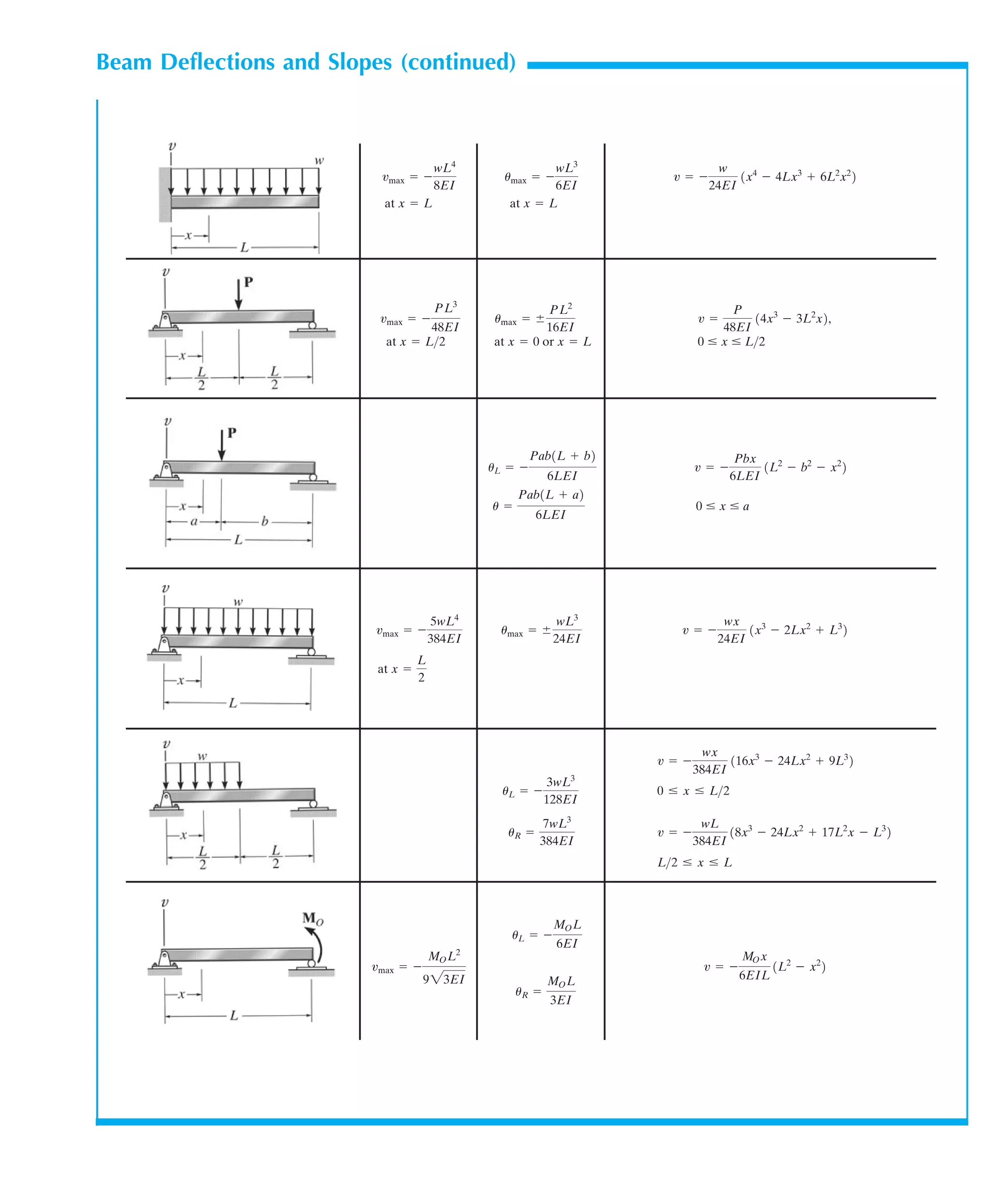
Tabulated Results. In the next section we will show how to apply
Eq. 8–4 to find the slope of a beam and the equation of its elastic curve.
The results from such an analysis for some common beam loadings often
encountered in structural analysis are given in the table on the inside
front cover of this book. Also listed are the slope and displacement at
critical points on the beam. Obviously, no single table can account for the
many different cases of loading and geometry that are encountered in
practice. When a table is not available or is incomplete, the displacement
or slope of a specific point on a beam or frame can be determined by using
the double integration method or one of the other methods discussed
in this and the next chapter.
ds = 2dx2
+ dv2
= 21 + 1dvdx22
dx L dx
dvdx L 0,
d2
v
dx2
=
M
EI
dvdx L 0.
v = f1x2,
M
EI
=
d2
vdx2
[1 + 1dvdx22
]32
1
r
=
d2
vdx2
[1 + 1dvdx22
]32
v
11r2
v
du =
M
EI
dx
dx = r du,

8.3 THE DOUBLE INTEGRATION METHOD 307
8
8.3 The Double Integration Method
Once M is expressed as a function of position x, then successive
integrations of Eq. 8–4 will yield the beam’s slope,
(Eq. 8–2), and the equation of the elastic curve,
respectively. For each integration it is
necessary to introduce a “constant of integration” and then solve for the
constants to obtain a unique solution for a particular problem. Recall
from Sec. 4–2 that if the loading on a beam is discontinuous—that is, it
consists of a series of several distributed and concentrated loads—then
several functions must be written for the internal moment, each valid
within the region between the discontinuities. For example, consider the
beam shown in Fig. 8–8. The internal moment in regions AB, BC, and
CD must be written in terms of the and coordinates. Once
these functions are integrated through the application of Eq. 8–4 and
the constants of integration determined, the functions will give the slope
and deflection (elastic curve) for each region of the beam for which
they are valid.
Sign Convention. When applying Eq. 8–4, it is important to use
the proper sign for M as established by the sign convention that was used
in the derivation of this equation, Fig. 8–9a. Furthermore, recall that
positive deflection, , is upward, and as a result, the positive slope angle
will be measured counterclockwise from the x axis.The reason for this is
shown in Fig. 8–9b. Here, positive increases dx and d in x and create
an increase that is counterclockwise.Also, since the slope angle will
be very small, its value in radians can be determined directly from
Boundary and Continuity Conditions. The constants of
integration are determined by evaluating the functions for slope or
displacement at a particular point on the beam where the value of the
function is known. These values are called boundary conditions. For
example, if the beam is supported by a roller or pin, then it is required
that the displacement be zero at these points.Also, at a fixed support the
slope and displacement are both zero.
If a single x coordinate cannot be used to express the equation for the
beam’s slope or the elastic curve, then continuity conditions must be
used to evaluate some of the integration constants. Consider the beam
in Fig. 8–10. Here the and coordinates are valid only within the
regions AB and BC, respectively. Once the functions for the slope and
deflection are obtained, they must give the same values for the slope and
deflection at point B, so that the elastic curve is physically
continuous. Expressed mathematically, this requires and
These equations can be used to determine two constants
of integration.
v11a2 = v21a2.
u11a2 = u21a2
x1 = x2 = a,
x2
x1
u L tan u = dvdx.
u
du
v
v
u
v
x3
x1, x2,
v = f1x2 = 1 11MEI2 dx,
11MEI2 dx
u L tan u = dvdx =
A D
P
w
x1
x2
x3
C
B
M M
(a)
v
x
dv
v
r
r
x
dx
O¿
u
du
elastic curve
ds
(b)
A
P
x1
x2
C
B
v1,v2
a b
v
u
Fig. 8–8
Fig. 8–9
Fig. 8–10

8
The following procedure provides a method for determining the
slope and deflection of a beam (or shaft) using the method of double
integration. It should be realized that this method is suitable only
for elastic deflections for which the beam’s slope is very small.
Furthermore, the method considers only deflections due to bending.
Additional deflection due to shear generally represents only a few
percent of the bending deflection, and so it is usually neglected in
engineering practice.
Elastic Curve
• Draw an exaggerated view of the beam’s elastic curve. Recall that
points of zero slope and zero displacement occur at a fixed
support, and zero displacement occurs at pin and roller supports.
• Establish the x and v coordinate axes. The x axis must be parallel
to the undeflected beam and its origin at the left side of the beam,
with a positive direction to the right.
• If several discontinuous loads are present, establish x coordi-
nates that are valid for each region of the beam between the
discontinuities.
• In all cases, the associated positive v axis should be directed
upward.
Load or Moment Function
• For each region in which there is an x coordinate, express the
internal moment M as a function of x.
• Always assume that M acts in the positive direction when apply-
ing the equation of moment equilibrium to determine
Slope and Elastic Curve
• Provided EI is constant, apply the moment equation
which requires two integrations. For each integration it is
important to include a constant of integration. The constants are
determined using the boundary conditions for the supports and the
continuity conditions that apply to slope and displacement at points
where two functions meet.
• Once the integration constants are determined and substituted
back into the slope and deflection equations, the slope and
displacement at specific points on the elastic curve can be deter-
mined.The numerical values obtained can be checked graphically
by comparing them with the sketch of the elastic curve.
• Positive values for slope are counterclockwise and positive
displacement is upward.
M(x),
EId2
vdx2
=
M = f(x).

EXAMPLE 8.3
Each simply supported floor joist shown in the photo is subjected to
a uniform design loading of 4 kN/m, Fig. 8–11a. Determine the
maximum deflection of the joist. EI is constant.
Elastic Curve. Due to symmetry, the joist’s maximum deflection
will occur at its center. Only a single x coordinate is needed to
determine the internal moment.
Moment Function. From the free-body diagram, Fig. 8–11b, we have
Slope and Elastic Curve. Applying Eq. 8–4 and integrating twice
gives
Here at so that , and at , so that
The equation of the elastic curve is therefore
At note that The maximum deflection is
therefore
Ans.
vmax = -
521
EI
dv/dx = 0.
x = 5 m,
EIv = 3.333x3
- 0.1667x4
- 166.7x
C1 = -166.7.
x = 10
v = 0
C2 = 0
x = 0
v = 0
EIv = 3.333x3
- 0.1667x4
+ C1x + C2
EI
dv
dx
= 10x2
- 0.6667x3
+ C1
EI
d2
v
dx2
= 20x - 2x2
M = 20x - 4xa
x
2
b = 20x - 2x2
4 kN/m
(a)
10 m
x
20 kN 20 kN
x
_
2
(4 x) N
(b)
x
20 kN
M
V
Fig. 8–11
8

8
The cantilevered beam shown in Fig. 8–12a is subjected to a couple
moment at its end. Determine the equation of the elastic curve.
EI is constant.
M0
EXAMPLE 8.4
SOLUTION
Elastic Curve. The load tends to deflect the beam as shown in
Fig. 8–9a. By inspection, the internal moment can be represented
throughout the beam using a single x coordinate.
Moment Function. From the free-body diagram, with M acting in
the positive direction, Fig. 8–12b, we have
Slope and Elastic Curve. Applying Eq. 8–4 and integrating twice
yields
(1)
(2)
(3)
Using the boundary conditions at and at
then Substituting these results into Eqs. (2) and
(3) with we get
Ans.
v =
M0x2
2EI
u =
M0x
EI
u = dvdx,
C1 = C2 = 0.
x = 0,
v = 0
x = 0
dvdx = 0
EIv =
M0x2
2
+ C1x + C2
EI
dv
dx
= M0x + C1
EI
d2
v
dx2
= M0
M = M0
L
x A
M0
(a)
x
M
M0
(b)
Fig. 8–12

8
Maximum slope and displacement occur at , for which
(4)
(5)
The positive result for indicates counterclockwise rotation and the
positive result for indicates that is upward. This agrees with the
results sketched in Fig. 8–12a.
In order to obtain some idea as to the actual magnitude of the slope
and displacement at the end A, consider the beam in Fig. 8–12a to
have a length of 12 ft, support a couple moment of and be
made of steel having If this beam were designed
without a factor of safety by assuming the allowable normal stress is
equal to the yield stress then a would be
found to be adequate From Eqs. (4) and (5) we get
Since this justifies the use of Eq. 8–4, rather
than applying the more exact Eq. 8–3, for computing the deflection of
beams. Also, since this numerical application is for a cantilevered
beam, we have obtained larger values for maximum and than
would have been obtained if the beam were supported using pins,
rollers, or other supports.
v
u
u2
A = 0.00297 rad2
V 1,
vA =
15 k # ft112 in.ft2112 ft22
112 in.1 ft22
21291103
2 kin2
2116.4 in4
2
= 3.92 in.
uA =
15 k # ft112 in.ft2112 ft2112 in.ft2
291103
2 kin2
116.4 in4
2
= 0.0545 rad
1I = 16.4 in.4
2.
W6 * 9
sallow = 36 ksi,
Est = 291103
2 ksi.
15 k # ft,
vA
vA
uA
vA =
M0L2
2EI
uA =
M0L
EI
A 1x = L2

8
The beam in Fig. 8–13a is subjected to a load P at its end. Determine
the displacement at C. EI is constant.
EXAMPLE 8.5
SOLUTION
Elastic Curve. The beam deflects into the shape shown in
Fig. 8–13a. Due to the loading, two x coordinates must be considered.
Moment Functions. Using the free-body diagrams shown in
Fig. 8–13b, we have
Slope and Elastic Curve. Applying Eq. 8–4,
for x1,
(1)
(2)
EIv1 = -
P
12
x3
1 + C1x1 + C2
EI
dv1
dx1
= -
P
4
x2
1 + C1
EI
d2
v1
dx2
1
= -
P
2
x1
= Px2 - 3Pa 2a … x2 … 3a
M2 = -
P
2
x2 +
3P
2
1x2 - 2a2
M1 = -
P
2
x1 0 … x1 … 2a
x2
A
P
C
B
2a a
x1
(a)
vC
V2
M2
x2
P
––
2 3P
___
2
2a
(b)
Fig. 8–13
x1
P
__
2
V1
M1

8
For x2,
(3)
(4)
The four constants of integration are determined using three bound-
ary conditions, namely, at at and
at and one continuity equation. Here the continuity of slope at
the roller requires at (Note that
continuity of displacement at B has been indirectly considered in the
boundary conditions, since at ) Applying
these four conditions yields
Solving, we obtain
Substituting and into Eq. (4) gives
The displacement at C is determined by setting We get
Ans.
vC = -
Pa3
EI
x2 = 3a.
v2 =
P
6EI
x3
2 -
3
2
Pa
EI
x2
2 +
10Pa2
3EI
x2 -
2Pa3
EI
C4
C3
C1 =
Pa2
3
C2 = 0 C3 =
10
3
Pa2
C4 = -2Pa3
-
P
4
12a22
+ C1 =
P
2
12a22
- 3Pa12a2 + C3
dv112a2
dx1
=
dv212a2
dx2
;
0 =
P
6
12a23
-
3
2
Pa12a22
+ C312a2 + C4
v2 = 0 at x2 = 2a;
0 = -
P
12
12a23
+ C112a2 + C2
v1 = 0 at x1 = 2a;
0 = 0 + 0 + C2
v1 = 0 at x1 = 0;
x1 = x2 = 2a.
v1 = v2 = 0
x1 = x2 = 2a.
dv1dx1 = dv2dx2
x2 = 2a,
v2 = 0
x1 = 2a,
x1 = 0, v1 = 0
v1 = 0
EIv2 =
P
6
x3
2 -
3
2
Pax2
2 + C3x2 + C4
EI
dv2
dx2
=
P
2
x2
2 - 3Pax2 + C3
EI
d2
v2
dx2
2
= Px2 - 3Pa

8
F8–4. Determine the equation of the elastic curve for the
beam using the x coordinate that is valid for EI
is constant.
0 6 x 6 L.
is constant.
0 6 x 6 L.
is constant.
0 6 x 6 L.
is constant.
0 6 x 6 L.
is constant.
0 6 x 6 L.
is constant.
0 6 x 6 L.
L
__
2
L
__
2
x
A B
P
L
__
2
L
__
2
x
A B
M0
A
L
B
M0
x
L
x
P
L
x
w0
F8–4
F8–5
F8–6
F8–7
F8–8
F8–9
w
L
x

8
8–2. The bar is supported by a roller constraint at B, which
allows vertical displacement but resists axial load and moment.
If the bar is subjected to the loading shown, determine the
slope at A and the deflection at C. EI is constant.
8–3. Determine the deflection at B of the bar in Prob. 8–2.
8–7. Determine the elastic curve for the simply supported
beam using the x coordinate Also, determine
the slope at A and the maximum deflection of the beam.
EI is constant.
0 … x … L2.
*8–4. Determine the equations of the elastic curve using the
coordinates and , specify the slope and deflection at B.
EI is constant.
8–5. Determine the equations of the elastic curve using the
coordinates and , and specify the slope and deflection
at point B. EI is constant.
x3
x1
x2
x1
*8–8. Determine the equations of the elastic curve using
the coordinates and , and specify the slope at C and
displacement at B. EI is constant.
8–9. Determine the equations of the elastic curve using
the coordinates and , and specify the slope at B and
deflection at C. EI is constant.
x3
x1
x2
x1
A B
P
P
L
x2
x1
a a
w
A
B
L L
x1 x2
C
L
x
A B
w0
L
A
B
a
w
x1
x2 x3
C
B
A
a
x1
x3
x2
a
w
C
P
A
C
B
L
2
L
2
8–1. Determine the equations of the elastic curve for the
beam using the and coordinates. Specify the slope at
A and the maximum deflection. EI is constant.
x2
x1
8–6. Determine the maximum deflection between the
supports A and B. EI is constant. Use the method of
integration.
PROBLEMS
Prob. 8–1
Probs. 8–2/8–3
Probs. 8–4/8–5
Prob. 8–7
Prob. 8–6
Probs. 8–8/8–9

8
8.4 Moment-Area Theorems
The initial ideas for the two moment-area theorems were developed by
Otto Mohr and later stated formally by Charles E. Greene in 1873.These
theorems provide a semigraphical technique for determining the slope of
the elastic curve and its deflection due to bending. They are particularly
advantageous when used to solve problems involving beams, especially
those subjected to a series of concentrated loadings or having segments
with different moments of inertia.
To develop the theorems, reference is made to the beam in Fig. 8–14a.
If we draw the moment diagram for the beam and then divide it by the
flexural rigidity, EI, the “M/EI diagram” shown in Fig. 8–14b results. By
Eq. 8–2,
Thus it can be seen that the change in the slope of the tangents on
either side of the element dx is equal to the lighter-shaded area under the
M/EI diagram. Integrating from point A on the elastic curve to point B,
Fig. 8–14c, we have
(8–5)
This equation forms the basis for the first moment-area theorem.
Theorem 1:The change in slope between any two points on the elastic
curve equals the area of the M/EI diagram between these two points.
The notation is referred to as the angle of the tangent at B
measured with respect to the tangent at A. From the proof it should be
evident that this angle is measured counterclockwise from tangent A to
tangent B if the area of the M/EI diagram is positive, Fig. 8–14c.
Conversely, if this area is negative, or below the x axis, the angle is
measured clockwise from tangent A to tangent B. Furthermore, from the
dimensions of Eq. 8–5, is measured in radians.
uBA
uBA
uBA
uBA =
L
B
A
M
EI
dx
du
du = a
M
EI
b dx
(a)
A B
w
x dx
M
___
EI M
___
EI
A B
x dx
(b)
x
A
B
elastic curve
tan B tan A
uB/A
(c)
Fig. 8–14

8.4 MOMENT-AREA THEOREMS 317
8
The second moment-area theorem is based on the relative deviation of
tangents to the elastic curve. Shown in Fig. 8–15c is a greatly exaggerated
view of the vertical deviation dt of the tangents on each side of the
differential element dx. This deviation is measured along a vertical line
passing through point A. Since the slope of the elastic curve and its
deflection are assumed to be very small, it is satisfactory to approximate
the length of each tangent line by x and the arc by dt. Using the
circular-arc formula where r is of length x,we can write
Using Eq. 8–2, the vertical deviation of the tangent at
A with respect to the tangent at B can be found by integration, in which
case
(8–6)
Recall from statics that the centroid of an area is determined from
Since represents an area of the M/EI dia-
gram, we can also write
(8–7)
Here is the distance from the vertical axis through A to the centroid of
the area between A and B, Fig. 8–15b.
The second moment-area theorem can now be stated as follows:
Theorem 2: The vertical deviation of the tangent at a point (A) on
the elastic curve with respect to the tangent extended from another
point (B) equals the “moment” of the area under the M/EI diagram
between the two points (A and B). This moment is computed about
point A (the point on the elastic curve), where the deviation is
to be determined.
Provided the moment of a positive M/EI area from A to B is
computed, as in Fig. 8–15b, it indicates that the tangent at point A is above
the tangent to the curve extended from point B, Fig. 8–15c. Similarly,
negative M/EI areas indicate that the tangent at A is below the tangent
extended from B. Note that in general is not equal to which is
shown in Fig. 8–15d. Specifically, the moment of the area under the M/EI
diagram between A and B is computed about point A to determine
Fig. 8–15b, and it is computed about point B to determine
It is important to realize that the moment-area theorems can only be
used to determine the angles or deviations between two tangents on the
beam’s elastic curve. In general, they do not give a direct solution for the
slope or displacement at a point on the beam.These unknowns must first
be related to the angles or vertical deviations of tangents at points on
the elastic curve. Usually the tangents at the supports are drawn in this
regard since these points do not undergo displacement and/or have zero
slope. Specific cases for establishing these geometric relationships are
given in the example problems.
tBA.
tAB,
tBA,
tAB
tAB
x
tAB = x
L
B
A
M
EI
dx
1MEI dx
x1dA = 1x dA.
tAB =
L
B
A
x
M
EI
dx
du = 1MEI2 dx,
dt = x du.
s = ur,
ds¿ (a)
A B
w
x dx
A B
_
x
(b)
x
M
___
EI
elastic curve
x dx
A B
tan A
ds¿
dt
tan B
(c)
tA/B
elastic curve
A
B
tan A
tA/B tB/A
tan B
(d)
Fig. 8–15

8
The following procedure provides a method that may be used to determine the
displacement and slope at a point on the elastic curve of a beam using the
moment-area theorems.
M/EI Diagram
• Determine the support reactions and draw the beam’s M/EI diagram.
• If the beam is loaded with concentrated forces, the M/EI diagram will consist of a
series of straight line segments, and the areas and their moments required for the
moment-area theorems will be relatively easy to compute.
• If the loading consists of a series of concentrated forces and distributed loads, it may
be simpler to compute the required M/EI areas and their moments by drawing the
M/EI diagram in parts, using the method of superposition as discussed in Sec. 4–5.
In any case, the M/EI diagram will consist of parabolic or perhaps higher-order
curves, and it is suggested that the table on the inside back cover be used to locate
the area and centroid under each curve.
Elastic Curve
• Draw an exaggerated view of the beam’s elastic curve. Recall that points of zero
slope occur at fixed supports and zero displacement occurs at all fixed, pin, and
roller supports.
• If it becomes difficult to draw the general shape of the elastic curve, use the
moment (or M/EI) diagram. Realize that when the beam is subjected to a positive
moment the beam bends concave up, whereas negative moment bends the beam
concave down. Furthermore, an inflection point or change in curvature occurs
where the moment in the beam (or M/EI) is zero.
• The displacement and slope to be determined should be indicated on the curve.
Since the moment-area theorems apply only between two tangents, attention
should be given as to which tangents should be constructed so that the angles or
deviations between them will lead to the solution of the problem. In this regard,
the tangents at the points of unknown slope and displacement and at the supports
should be considered, since the beam usually has zero displacement and/or zero
slope at the supports.
Moment-Area Theorems
• Apply Theorem 1 to determine the angle between two tangents, and Theorem 2
to determine vertical deviations between these tangents.
• Realize that Theorem 2 in general will not yield the displacement of a point on the
elastic curve. When applied properly, it will only give the vertical distance or
deviation of a tangent at point A on the elastic curve from the tangent at B.
• After applying either Theorem 1 or Theorem 2, the algebraic sign of the answer
can be verified from the angle or deviation as indicated on the elastic curve.

8
15 ft 15 ft
M
––
EI
A
B C
x
60
__
EI
30
__
EI
(b)
tan B
A
tan C
tan A
C
B
uB/A
uC/A
(c)
uB
uC
EXAMPLE 8.6
Determine the slope at points B and C of the beam shown in Fig. 8–16a.
Take and
SOLUTION
M/EI Diagram. This diagram is shown in Fig. 8–16b. It is easier to
solve the problem in terms of EI and substitute the numerical data as
a last step.
Elastic Curve. The 2-k load causes the beam to deflect as shown in
Fig. 8–16c. (The beam is deflected concave down, since M/EI is
negative.) Here the tangent at A (the support) is always horizontal.
The tangents at B and C are also indicated.We are required to find
and . By the construction, the angle between tan A and tan B, that
is, is equivalent to
Also,
Moment-Area Theorem. Applying Theorem 1, is equal to the
area under the M/EI diagram between points A and B; that is,
Substituting numerical data for E and I, and converting feet to inches,
we have
Ans.
The negative sign indicates that the angle is measured clockwise from
A, Fig. 8–16c.
In a similar manner, the area under the M/EI diagram between
points A and C equals We have
Substituting numerical values for EI, we have
Ans.
= -0.00745 rad
uC =
-900 k # ft2
1144 in2
ft2
2
291103
2 kin2
1600 in4
2
uC = uCA =
1
2
a -
60 k # ft
EI
b130 ft2 = -
900 k # ft2
EI
uCA.
= -0.00559 rad
uB =
-675 k # ft2
1144 in2
1 ft2
2
291103
2 kin2
1600 in4
2
= -
675 k # ft2
EI
uB = uBA = - a
30 k # ft
EI
b115 ft2 -
1
2
a
60 k # ft
EI
-
30 k # ft
EI
b115 ft2
uBA
uC = uCA
uB = uBA
uB.
uBA,
uC
uB
I = 600in4
.
E = 291103
2 ksi
Fig. 8–16
2 k
A
C
B
30 ft
15 ft
(a)

8
Determine the deflection at points B and C of the beam shown in
Fig. 8–17a. Values for the moment of inertia of each segment are
indicated in the figure.Take
SOLUTION
M/EI Diagram. By inspection, the moment diagram for the beam is
a rectangle. Here we will construct the M/EI diagram relative to ,
realizing that . Fig. 8–17b. Numerical data for will be
substituted as a last step.
Elastic Curve. The couple moment at C causes the beam to deflect
as shown in Fig. 8–17c. The tangents at A (the support), B, and C are
indicated. We are required to find and . These displacements
can be related directly to the deviations between the tangents, so that
from the construction is equal to the deviation of tan B relative to
tan A; that is,
Also,
Moment-Area Theorem. Applying Theorem 2, is equal to the
moment of the area under the diagram between A and B
computed about point B, since this is the point where the tangential
deviation is to be determined. Hence, from Fig. 8–17b,
Substituting the numerical data yields
Ans.
Likewise, for we must compute the moment of the entire
diagram from A to C about point C.We have
Ans.
Since both answers are positive, they indicate that points B and C lie
above the tangent at A.
= 0.00906 m = 9.06 mm
=
7250 N # m3
EIBC
=
7250 N # m3
[2001109
2 Nm2
][41106
2110-12
2 m4
]
¢C = tCA = c
250 N # m
EIBC
14 m2d15 m2 + c
500 N # m
EIBC
13 m2d11.5 m2
MEIBC
tCA
= 0.0025 m = 2.5 mm.
¢B =
2000 N # m3
[2001109
2 Nm2
][41106
2 mm4
11 m4
1103
24
mm4
2]
¢B = tBA = c
250 N # m
EIBC
14 m2d12 m2 =
2000 N # m3
EIBC
MEIBC
tBA
¢C = tCA
¢B = tBA
¢B
¢C
¢B
EIBC
IAB = 2IBC
IBC
E = 200 GPa.
EXAMPLE 8.7
(a)
4 m
IAB 8(106
) mm4
3 m
IBC 4(106
)mm4
A
B C 500 Nm
4 m
2 m
3 m
A B C
250
____
EIBC
M
____
EIBC
500
____
EIBC
x
(b)
tan B
A
tan A
B tB/A
B
Ctan C
C tC/A
(c)
Fig. 8–17

8
EXAMPLE 8.8
Determine the slope at point C of the beam in Fig. 8–18a.
,
SOLUTION
M/EI Diagram. Fig. 8–18b.
Elastic Curve. Since the loading is applied symmetrically to the
beam, the elastic curve is symmetric, as shown in Fig. 8–18c. We are
required to find This can easily be done, realizing that the tangent
at D is horizontal, and therefore, by the construction, the angle
between tan C and tan D is equal to that is,
Moment-Area Theorem. Using Theorem 1, is equal to the
shaded area under the M/EI diagram between points C and D. We
have
Thus,
Ans.
uC =
135 kN # m2
[2001106
2 kNm2
][61106
2110-12
2 m4
]
= 0.112 rad
=
135 kN # m2
EI
uC = uDC = 3 ma
30 kN # m
EI
b +
1
2
13 m2a
60 kN # m
EI
-
30 kN # m
EI
b
uDC
uC = uDC
uC;
uDC
uC.
I = 6(106
) mm4
.
E = 200 GPa
uD/C
horizontal
tan D
tan C
D
C
uC
(c)
3 m
(b)
C D
x
M
___
EI 60
___
EI
30
___
EI
A B
3 m 6 m
Fig. 8–18
20 kN
3 m 3 m 6 m
C D
(a)
A
B

8 k
6 ft 12 ft 6 ft
C
(a)
A
B
8
Determine the slope at point C of the beam in Fig. 8–19a.
,
SOLUTION
Elastic Curve. The elastic curve is shown in Fig. 8–19c. We are
required to find To do this, establish tangents at A, B (the
supports), and C and note that is the angle between the tangents
at A and C. Also, the angle in Fig. 8–19c can be found using
This equation is valid since is actually very small,
so that can be approximated by the length of a circular arc
defined by a radius of and sweep of . (Recall that .)
From the geometry of Fig. 8–19c, we have
(1)
Moment-Area Theorems. Using Theorem 1, is equivalent to
the area under the M/EI diagram between points A and C; that is,
Applying Theorem 2, is equivalent to the moment of the area
under the M/EI diagram between B and A about point B, since this is
the point where the tangential deviation is to be determined.We have
Substituting these results into Eq. 1, we have
so that
Ans.
= 0.00119 rad
uC =
144 k # ft2
291103
2 kin2
1144 in2
ft2
2 600 in4
11 ft4
11224
in4
2
uC =
4320 k # ft3
124 ft2 EI
-
36 k # ft2
EI
=
144 k # ft2
EI
=
4320 k # ft3
EI
+
2
3
16 ft2c
1
2
16 ft2a
36 k # ft
EI
b d
tBA = c6 ft +
1
3
118 ft2d c
1
2
118 ft2a
36 k # ft
EI
b d
tBA
uCA =
1
2
16 ft2a
12 k # ft
EI
b =
36 k # ft2
EI
uCA
uC = f - uCA =
tBA
24
- uCA
s = ur
f
LAB = 24 ft
tBA
tBA
f = tBALAB.
f
uCA
uC.
I = 600 in4
.
E = 29(103
) ksi
EXAMPLE 8.9
(b)
x
M
___
EI
36
___
EI
12
___
EI
6 ft 6 ft
12 ft
tan B
tan C
C
uC
(c)
A
uC/A
tB/A
B
tan A
f
Fig. 8–19

8
Fig. 8–20
EXAMPLE 8.10
Determine the deflection at C of the beam shown in Fig. 8–20a. Take
SOLUTION
Elastic Curve. Here we are required to find Fig. 8–20c. This is
not necessarily the maximum deflection of the beam, since the loading
and hence the elastic curve are not symmetric. Also indicated in
Fig. 8–20c are the tangents at A, B (the supports), and C. If is
determined, then can be found from proportional triangles, that is,
or From the construction in Fig. 8–20c,
we have
(1)
Moment-Area Theorem. We will apply Theorem 2 to determine
and Here is the moment of the M/EI diagram between
A and B about point A,
and is the moment of the M/EI diagram between C and B about C.
Substituting these results into Eq. (1) yields
Working in units of kips and inches, we have
Ans.
= 0.511 in.
¢C =
180 k # ft3
11728 in3
ft3
2
291103
2 kin2
121 in4
2
¢C =
1
2
a
480 k # ft3
EI
b -
60 k # ft3
EI
=
180 k # ft3
EI
tCB = c
1
3
112 ft2d c
1
2
112 ft2a
2.5 k # ft
EI
b d =
60 k # ft3
EI
tCB
tAB = c
1
3
124 ft2d c
1
2
124 ft2a
5 k # ft
EI
b d =
480 k # ft3
EI
tAB
tCB.
tAB
¢C =
tAB
2
- tCB
¢¿ = tAB2.
¢¿12 = tAB24
¢¿
tAB
¢C,
E = 29(103
) ksi, I = 21 in4
.
A
5 kft
12 ft 12 ft
C
(a)
B
(b)
x
M
___
EI
2.5
___
EI
5
___
EI
12 ft 12 ft
12 ft 12 ft
C
C
tan A
A
tan C
B
tan B
tC/B
¿
tA/B
(c)

8
EXAMPLE 8.11
M
___
EI
8 m 8 m
x
192
___
EI
(b)
C
¿
tC/A
tan A
tan C
tan B tB/A
A
B
C
(c)
6 kN/m
8 m 8 m
C
A
B
(a)
24 kN
72 kN
Fig. 8–21
Determine the deflection at point C of the beam shown in Fig. 8–21a.
SOLUTION
M/EI Diagram. As shown in Fig. 8–21b, this diagram consists of a
triangular and a parabolic segment.
Elastic Curve. The loading causes the beam to deform as shown in
Fig. 8–21c.We are required to find By constructing tangents at A,
B (the supports), and C, it is seen that However,
can be related to by proportional triangles, that is,
or Hence
(1)
Moment-Area Theorem. We will apply Theorem 2 to determine
and Using the table on the inside back cover for the
parabolic segment and considering the moment of the M/EI diagram
between A and C about point C, we have
The moment of the M/EI diagram between A and B about point B gives
Why are these terms negative? Substituting the results into Eq.(1) yields
Thus,
Ans.
= -0.143 m
¢C =
-7168 kN # m3
[2001106
2 kNm2
][2501106
2110-12
2 m4
]
= -
7168 kN # m3
EI
¢C = -
11 264 kN # m3
EI
- 2a-
2048 kN # m3
EI
b
tBA = c
1
3
18 m2d c
1
2
18 m2a-
192 kN # m
EI
b d = -
2048 kN # m3
EI
= -
11 264 kN # m3
EI
+ c
1
3
18 m2 + 8 md c
1
2
18 m2a-
192 kN # m
EI
b d
tCA = c
3
4
18 m2d c
1
3
18 m2a-
192 kN # m
EI
b d
tBA.
tCA
¢C = tCA - 2tBA
¢¿ = 2tBA.
¢¿16 = tBA8
tBA
¢¿
¢C = tCA - ¢¿.
¢C.
E = 200 GPa, I = 250(106
) mm4
.

8
EXAMPLE 8.12
Determine the slope at the roller B of the double overhang beam
shown in Fig. 8–22a.Take
SOLUTION
M/EI Diagram. The M/EI diagram can be simplified by drawing it
in parts and considering the M/EI diagrams for the three loadings
each acting on a cantilever beam fixed at D, Fig. 8–22b. (The 10-kN
load is not considered since it produces no moment about D.)
Elastic Curve. If tangents are drawn at B and C, Fig. 8–22c, the
slope B can be determined by finding and for small angles,
(1)
Moment Area Theorem. To determine we apply the moment
area theorem by finding the moment of the M/EI diagram between
BC about point C.This only involves the shaded area under two of the
diagrams in Fig. 8–22b.Thus,
Substituting into Eq. (1),
Ans.
= 0.00741 rad
uB =
53.33 kN # m3
12 m2[2001106
2 kNm3
][181106
2110-12
2 m4
]
=
53.33 kN # m3
EI
tCB = 11 m2c12 m2a
-30 kN # m
EI
b d + a
2 m
3
b c
1
2
12 m2a
10 kN # m
EI
b d
tCB
uB =
tCB
2 m
tCB,
E = 200 GPa, I = 18(106
) mm4
.
A
30 kNm
10 kN
2 m 2 m
5 kN 5 kN
2 m
B C
(a)
D
(b)
2 4 6
x
2
+
+
4 6
x
4 6
x
M
—
EI
M
—
EI
10
—
EI
20
—
EI
–30
–—
EI
10
—
EI
M
—
EI
(c)
2 m
tC/B
tan C
tan B
uB
uB
Fig. 8–22

8
8.5 Conjugate-Beam Method
The conjugate-beam method was developed by H. Müller-Breslau in
1865. Essentially, it requires the same amount of computation as the
moment-area theorems to determine a beam’s slope or deflection;
however, this method relies only on the principles of statics, and hence
its application will be more familiar.
The basis for the method comes from the similarity of Eq. 4–1 and
Eq. 4–2 to Eq. 8–2 and Eq. 8–4.To show this similarity, we can write these
equations as follows:
Or integrating,
Here the shear V compares with the slope the moment M compares
with the displacement , and the external load w compares with the M/EI
diagram. To make use of this comparison we will now consider a beam
having the same length as the real beam, but referred to here as the
“conjugate beam,” Fig. 8–23. The conjugate beam is “loaded” with
the M/EI diagram derived from the load w on the real beam. From the
above comparisons, we can state two theorems related to the conjugate
beam, namely,
Theorem 1: The slope at a point in the real beam is numerically
equal to the shear at the corresponding point in the conjugate beam.
Theorem 2: The displacement of a point in the real beam is
numerically equal to the moment at the corresponding point in the
conjugate beam.
Conjugate-Beam Supports. When drawing the conjugate beam
it is important that the shear and moment developed at the supports of the
conjugate beam account for the corresponding slope and displacement of
the real beam at its supports, a consequence of Theorems 1 and 2. For
v
u,
V =
L
w dx
D D
u =
L
a
M
EI
b dx
5
M =
L
c
L
w dx d dx
D D
v =
L
c
L
a
M
EI
b dx d dx
dV
dx
= w
du
dx
=
M
EI
4
d2
M
dx2
= w
d2
v
dx2
=
M
EI
L
L
A B
w
real beam
A¿ B¿
conjugate beam
M
___
EI
Fig. 8–23

8.5 CONJUGATE-BEAM METHOD 327
8
example, as shown in Table 8–2, a pin or roller support at the end of the
real beam provides zero displacement, but the beam has a nonzero slope.
Consequently, from Theorems 1 and 2, the conjugate beam must be
supported by a pin or roller, since this support has zero moment but has
a shear or end reaction. When the real beam is fixed supported (3), both
the slope and displacement at the support are zero. Here the conjugate
beam has a free end, since at this end there is zero shear and zero moment.
Corresponding real and conjugate-beam supports for other cases are listed
in the table. Examples of real and conjugate beams are shown in Fig. 8–24.
Note that, as a rule, neglecting axial force, statically determinate real
beams have statically determinate conjugate beams; and statically
indeterminate real beams, as in the last case in Fig. 8–24, become unstable
conjugate beams. Although this occurs, the M/EI loading will provide the
necessary “equilibrium” to hold the conjugate beam stable.
TABLE 8–2
Real Beam Conjugate Beam
1)
2)
3)
4)
5)
6)
7)
0
pin
0
roller
0
fixed
free
internal pin
internal roller
hinge
M 0
V
pin
M 0
V
roller
M 0
V 0
free
M
V
fixed
M 0
V
hinge
M 0
V
hinge
M
V
internal roller
u
u
u
u 0
0
u
0
u

u

8
Fig. 8–24
real beam conjugate beam
The following procedure provides a method that may be used to determine the
displacement and slope at a point on the elastic curve of a beam using the
conjugate-beam method.
Conjugate Beam
• Draw the conjugate beam for the real beam. This beam has the same length as
the real beam and has corresponding supports as listed in Table 8–2.
• In general, if the real support allows a slope, the conjugate support must develop a
shear; and if the real support allows a displacement, the conjugate support must
develop a moment.
• The conjugate beam is loaded with the real beam’s M/EI diagram. This loading is
assumed to be distributed over the conjugate beam and is directed upward when
M/EI is positive and downward when M/EI is negative. In other words, the loading
always acts away from the beam.
Equilibrium
• Using the equations of equilibrium, determine the reactions at the conjugate
beam’s supports.
• Section the conjugate beam at the point where the slope and displacement of
the real beam are to be determined. At the section show the unknown shear
and moment acting in their positive sense.
• Determine the shear and moment using the equations of equilibrium. and
equal and , respectively, for the real beam. In particular, if these values are
positive, the slope is counterclockwise and the displacement is upward.
¢
u
M¿
V¿
M¿
V¿
¢
u

8
EXAMPLE 8.13
Determine the slope and deflection at point B of the steel beam
shown in Fig. 8–25a. The reactions have been computed.
SOLUTION
Conjugate Beam. The conjugate beam is shown in Fig. 8–25b. The
supports at and correspond to supports A and B on the real
beam,Table 8–2. It is important to understand why this is so.The M/EI
diagram is negative, so the distributed load acts downward, i.e., away
from the beam.
Equilibrium. Since and are to be determined, we must
compute and in the conjugate beam, Fig. 8–25c.
Ans.
Ans.
The negative signs indicate the slope of the beam is measured
clockwise and the displacement is downward, Fig. 8–25d.
= -0.0873 ft = -1.05 in.
=
-14 062.5 k # ft3
291103
211442 kft2
[80011224
] ft4
¢B = MB¿ = -
14 062.5 k # ft3
EI
562.5 k # ft2
EI
125 ft2 + MB¿ = 0
d+©MB¿ = 0;
= -0.00349 rad
=
-562.5 k # ft2
291103
2 kin2
1144 in2
ft2
2800 in4
11 ft4
11224
in4
2
uB = VB¿ = -
562.5 k # ft2
EI
-
562.5 k # ft2
EI
- VB¿ = 0
+ c©Fy = 0;
MB¿
VB¿
¢B
uB
B¿
A¿
I = 800 in4
.
E = 29(103
) ksi,
5 k
15 ft 15 ft
A
B
75 kft
real beam
(a)
5 k
15 ft 15 ft
A¿ B¿
75
__
EI
conjugate beam
(b)
5 ft 25 ft
562.5
_____
EI
MB¿
VB¿
reactions
(c)
A
B
(d)
uB
B
Fig. 8–25

8
Determine the maximum deflection of the steel beam shown in
Fig. 8–26a. The reactions have been computed.
SOLUTION
Conjugate Beam. The conjugate beam loaded with the M/EI
diagram is shown in Fig. 8–26b. Since the M/EI diagram is positive, the
distributed load acts upward (away from the beam).
Equilibrium. The external reactions on the conjugate beam are
determined first and are indicated on the free-body diagram in
Fig. 8–26c. Maximum deflection of the real beam occurs at the point
where the slope of the beam is zero. This corresponds to the same
point in the conjugate beam where the shear is zero. Assuming this
point acts within the region from , we can isolate the
section shown in Fig. 8–26d. Note that the peak of the distributed
loading was determined from proportional triangles, that is,
We require so that
Using this value for x, the maximum deflection in the real beam corre-
sponds to the moment . Hence,
Ans.
The negative sign indicates the deflection is downward.
= -0.0168 m = -16.8 mm
=
-201.2 kN # m3
[2001106
2 kNm2
][601106
2 mm4
11 m4
1103
24
mm4
2]
¢max = M¿ = -
201.2 kN # m3
EI
45
EI
16.712 - c
1
2
a
216.712
EI
b6.71d
1
3
16.712 + M¿ = 0
d+©M = 0;
M¿
x = 6.71 m 10 … x … 9 m2 OK
-
45
EI
+
1
2
a
2x
EI
bx = 0
+ c©Fy = 0;
V¿ = 0
wx = (18EI)9.
A¿
0 … x … 9 m
I = 60(106
) mm4
.
E = 200 GPa,
EXAMPLE 8.14
6 m
external reactions
(c)
81
__
EI
4 m 2 m
27
__
EI
45
__
EI
63
__
EI
18 x 2x
__ (_) __
EI 9 EI
M¿
A¿
x
internal reactions
(d)
45
__
EI
V¿ 0
9 m 3 m
8 kN
2 kN 6 kN
real beam
(a)
B
18
__
EI
9 m 3 m
conjugate beam
(b)
A¿ B¿
Fig. 8–26

12 18 24 36
120 120
144
M (kft)
x (ft)
moment diagram
(b)
8
EXAMPLE 8.15
The girder in Fig.8–27a is made from a continuous beam and reinforced
at its center with cover plates where its moment of inertia is larger.
The 12-ft end segments have a moment of inertia of and
the center portion has a moment of inertia of Determine
the deflection at the center C. Take The reactions
have been calculated.
SOLUTION
Conjugate Beam. The moment diagram for the beam is determined
first,Fig.8–27b.Since for simplicity,we can express the load on
the conjugate beam in terms of the constant EI, as shown in Fig. 8–27c.
Equilibrium. The reactions on the conjugate beam can be calculated
by the symmetry of the loading or using the equations of equilibrium.
The results are shown in Fig. 8–27d. Since the deflection at C is to be
determined, we must compute the internal moment at . Using
the method of sections, segment is isolated and the resultants of
the distributed loads and their locations are determined,Fig.8–27e.Thus,
Substituting the numerical data for EI and converting units, we have
Ans.
The negative sign indicates that the deflection is downward.
¢C = MC¿ = -
11 736 k # ft3
11728 in3
ft3
2
291103
2 kin2
1450 in4
2
= -1.55 in.
MC¿ = -
11 736 k # ft3
EI
1116
EI
1182 -
720
EI
1102 -
360
EI
132 -
36
EI
122 + MC¿ = 0
d+©MC¿ = 0;
A¿C¿
C¿
I¿ = 2I,
E = 29(103
) ksi.
I¿ = 900 in4
.
I = 450 in4
,
12 ft 12 ft
6 ft 6 ft
6 k 8 k 6 k
10 k 10 k
I¿ = 900 in4
I = 450 in4 I = 450 in4
A B
C
C
real beam
(a)
120
___
EI
60
___
EI
72
___
EI
60
___
EI
120
___
EI
12 ft 12 ft
6 ft 6 ft
C¿
A¿ B¿
conjugate beam
(c)
8 ft
720
___
EI 72
___
EI
A¿ B¿
external reactions
(d)
8 ft
10 ft
10 ft
720
___
EI
720
___
EI
1116
____
EI
1116
____
EI
18 ft
720
___
EI
36
___
EI
A¿
C¿
internal reactions
(e)
10 ft
1116
____
EI
360
___
EI
3 ft
2 ft
VC¿
MC¿
Fig. 8–27

8
Fig. 8–28
Determine the displacement of the pin at B and the slope of each
beam segment connected to the pin for the compound beam shown in
Fig. 8–28a.
SOLUTION
Conjugate Beam. The elastic curve for the beam is shown in
Fig. 8–28b in order to identify the unknown displacement and the
slopes and to the left and right of the pin. Using Table 8–2,
the conjugate beam is shown in Fig. 8–28c. For simplicity in calculation,
the M/EI diagram has been drawn in parts using the principle of
superposition as described in Sec. 4–5. In this regard, the real beam is
thought of as cantilevered from the left support, A. The moment
diagrams for the 8-k load, the reactive force and the
loading are given. Notice that negative regions of this diagram
develop a downward distributed load and positive regions have a
distributed load that acts upward.
30-k # ft
Cy = 2 k,
(uB)R
(uB)L
¢B
E = 29(103
) ksi, I = 30 in4
.
EXAMPLE 8.16
12 ft
8 k
real beam
(a)
A B
12 ft 15 ft
C
30 kft
A
8 k
C
30 kft
elastic curve
(b)
B
B
(uB)R (uB)L
78
–––
EI
15 ft
B¿
conjugate beam
(c)
12 ft 12 ft
A¿ C¿
30
–––
EI
96
–––
EI
B¿
external reactions
(d)
11 ft
576
___
EI
20 ft
228.6
_____
EI
1170
____
EI 15 ft
4.5 ft
3.6
___
EI
1521
____
EI

8
(e)
MB¿
(VB¿)R
15 ft
7.5 ft
5 ft
3.6
___
EI
225
___
EI
450
___
EI
B¿
(f)
15 ft
7.5 ft
5 ft
225
___
EI
450
___
EI
MB¿
(VB¿)L
B¿
228.6
____
EI
3.6
___
EI
Equilibrium. The external reactions at and are calculated first
and the results are indicated in Fig. 8–28d. In order to determine
the conjugate beam is sectioned just to the right of and the
shear force is computed, Fig. 8–28e.Thus,
Ans.
The internal moment at yields the displacement of the pin.Thus,
Ans.
The slope can be found from a section of beam just to the left
of , Fig. 8–28f.Thus,
Ans.
Obviously, for this segment is the same as previously
calculated,since the moment arms are only slightly different in Figs. 8–28e
and 8–28f.
¢B = MB¿
1uB2L = 1VB¿2L = 0
1VB¿2L +
228.6
EI
+
225
EI
-
450
EI
-
3.6
EI
= 0
+ c ©Fy = 0;
B¿
(uB)L
= -0.381 ft = -4.58 in.
=
-2304 k # ft3
[291103
211442 kft2
][3011224
] ft4
¢B = MB¿ = -
2304 k # ft3
EI
-MB¿ +
225
EI
152 -
450
EI
17.52 -
3.6
EI
1152 = 0
d+©MB¿ = 0;
B¿
= 0.0378 rad
=
228.6 k # ft2
[291103
211442 kft2
][3011224
] ft4
1uB2R = 1VB¿2R =
228.6 k # ft2
EI
1VB¿2R +
225
EI
-
450
EI
-
3.6
EI
= 0
+ c ©Fy = 0;
(VB¿)R
B¿
(uB)R,
C¿
B¿

8
F8–10. Use the moment-area theorems and determine the
slope at A and deflection at A. EI is constant.
F8–11. Solve Prob. F8–10 using the conjugate beam
method.
slope at A and displacement at C. EI is constant.
method.
slope at B and deflection at B. EI is constant.
method.
method.
method.
slope at B and displacement at B. EI is constant.
method.
3 m
A B
6 kN
F8–10/8–11
A
4 m
B
8 kNm
F8–12/8–13
A
C
B
5 kNm
1.5 m 1.5 m
F8–14/8–15
A
8 kN
C
3 m 3 m
B
F8–16/8–17
A
4 kN 4 kN
2 m 2 m
4 m 4 m
B
C
F8–18/8–19
A
2 m 2 m
9 kN
B
F8–20/8–21

8
*8–12. Determine the slope and displacement at C. EI is
constant. Use the moment-area theorems.
8–13. Solve Prob. 8–12 using the conjugate-beam method.
8–10. Determine the slope at B and the maximum
displacement of the beam. Use the moment-area theorems.
Take
E = 29(103
) ksi, I = 500 in4
.
8–14. Determine the value of a so that the slope at A is
equal to zero. EI is constant. Use the moment-area theorems.
*8–16. Determine the value of a so that the displacement
at C is equal to zero. EI is constant. Use the moment-area
theorems.
PROBLEMS
6 ft 6 ft
A
B
C
15 k
Probs. 8–10/8–11
A
B
C
15 ft
15 k
30 ft
Probs. 8–12/8–13
A D
P
B
C
P
a L
__
2
L
__
2
Probs. 8–14/8–15/8–16/8–17
a a a
B
A C
P
Probs. 8–18/8–19
8–18. Determine the slope and the displacement at C. EI
is constant. Use the moment-area theorems.
*8–20. Determine the slope and the displacement at the
end C of the beam. Use
the moment-area theorems.
E = 200 GPa, I = 70(106
) mm4
.
B
D
A C
3 m 3 m
8 kN
4 kN
3 m
Probs. 8–20/8–21
8–22. At what distance a should the bearing supports at A
and B be placed so that the displacement at the center of
the shaft is equal to the deflection at its ends? The bearings
exert only vertical reactions on the shaft. EI is constant. Use
the moment-area theorems.
A B
a
L
P
P
a
Probs. 8–22/8–23

8
8–29. Determine the force F at the end of the beam C so
that the displacement at C is zero. EI is constant. Use the
conjugate-beam method.
8–26. Determine the displacement at C and the slope at B.
EI is constant. Use the moment-area theorems.
*8–28. Determine the force F at the end of the beam C so
that the displacement at C is zero. EI is constant. Use the
moment-area theorems.
*8–24. Determine the displacement at C and the slope
at B. EI is constant. Use the moment-area theorems.
8–25. Solve Prob. 8–24 using the conjugate-beam
method.
A B
C
3 m 1.5 m 1.5 m
4 kN
4 kN
3 m
Probs. 8–24/8–25
A C B
P
P
a a a a
2
P
2
Prob. 8–26
A C B
P
P
a a a a
2
P
2
Prob. 8–27
a a a
B
D
A C
P
F
Prob. 8–28
a a a
B
D
A C
P
F
Prob. 8–29
a a a
A
C
P P
B
Prob. 8–30
8–30. Determine the slope at B and the displacement at C.
EI is constant. Use the moment-area theorems.
a a a
A
C
P P
B
Prob. 8–31
8–31. Determine the slope at B and the displacement at C.
EI is constant. Use the conjugate-beam method.
8–27. Determine the displacement at C and the slope at B.
EI is constant. Use the conjugate-beam method.

8
*8–32. Determine the maximum displacement and the slope
at A. EI is constant. Use the moment-area theorems.
8–38. Determine the displacement at D and the slope at
D. Assume A is a fixed support, B is a pin, and C is a roller.
Use the moment-area theorems.
A
M0
C
B
L
__
2
L
__
2
Prob. 8–32
A
M0
C
B
L
__
2
L
__
2
Prob. 8–33
a
a
A C
P
B
M0 Pa
Prob. 8–35
a
a
A C
P
B
M0 Pa
Prob. 8–34
3 m 3 m
25 kN
3 m
A B
D
C
Prob. 8–36
3 m 3 m
25 kN
3 m
A B
D
C
Prob. 8–37
12 ft 12 ft 12 ft
A B C D
6 k
Prob. 8–38
12 ft 12 ft 12 ft
A B C D
6 k
Prob. 8–39
8–35. Determine the slope and displacement at C. EI is
constant. Use the conjugate-beam method.
8–39. Determine the displacement at D and the slope at
D. Assume A is a fixed support, B is a pin, and C is a roller.
Use the conjugate-beam method.
*8–36. Determine the displacement at C. Assume A is a
fixed support, B is a pin, and D is a roller. EI is constant.
Use the moment-area theorems.
8–37. Determine the displacement at C. Assume A is a
fixed support, B is a pin, and D is a roller. EI is constant.
Use the conjugate-beam method.
8–33. Determine the maximum displacement at B and the
slope at A. EI is constant. Use the conjugate-beam method.
8–34. Determine the slope and displacement at C. EI is
constant. Use the moment-area theorems.

8
The deflection of a member (or structure) can always
be established provided the moment diagram is
known, because positive moment will tend to bend the
member concave upwards, and negative moment
will tend to bend the member concave downwards.
Likewise, the general shape of the moment diagram
can be determined if the deflection curve is known.
CHAPTER REVIEW
Deflection of a beam due to bending can be
determined by using double integration of the
equation.
Here the internal moment M must be expressed as a
function of the x coordinates that extend across the
beam. The constants of integration are obtained from
the boundary conditions, such as zero deflection at a
pin or roller support and zero deflection and slope at a
fixed support. If several x coordinates are necessary,
then the continuity of slope and deflection must be
considered, where at and
.
v1(a) = v2(a)
u1(a) = u2(a)
x1 = x2 = a,
d2
v
dx2
=
M
EI
beam
P1
P2
P
x1
x2
v1,v2
a b
v
u
M
x
moment diagram
inflection point
deflection curve

CHAPTER REVIEW 339
8
If the moment diagram has a simple shape, the moment-area theorems or the conjugate beam method can be used to
determine the deflection and slope at a point on the beam.
The moment-area theorems consider the angles and vertical deviation between the tangents at two points A and B
on the elastic curve. The change in slope is found from the area under the M/EI diagram between the two points, and the
deviation is determined from the moment of the M/EI diagram area about the point where the deviation occurs.
The conjugate beam method is very methodical and requires application of the principles of statics. Quite simply, one
establishes the conjugate beam using Table 8–2, then considers the loading as the M/EI diagram. The slope (deflection) at
a point on the real beam is then equal to the shear (moment) at the same point on the conjugate beam.
A B
w
A
B
uB/A Area of M/EI diagram
tan B tan A
uB/A
A B
_
x
Area
x
M
___
EI
A
B
tan A
tA/B tB/A
tan B
tA/B (Area of M/EI diagram)
_
x
L
A B
w
real beam
L
A¿ B¿
conjugate beam
M
___
EI

The displacement at the ends of this bridge deck, as it is being constructed,
can be determined using energy methods.

9
341
In this chapter, we will show how to apply energy methods to solve problems
involving slope and deflection. The chapter begins with a discussion of work
and strain energy, followed by a development of the principle of work and
energy. The method of virtual work and Castigliano’s theorem are then
developed, and these methods are used to determine the displacements at
points on trusses, beams, and frames.
9.1 External Work and Strain Energy
The semigraphical methods presented in the previous chapters are very
effective for finding the displacements and slopes at points in beams
subjected to rather simple loadings. For more complicated loadings or
for structures such as trusses and frames, it is suggested that energy
methods be used for the computations. Most energy methods are based
on the conservation of energy principle, which states that the work done
by all the external forces acting on a structure, is transformed
into internal work or strain energy, which is developed when
the structure deforms. If the material’s elastic limit is not exceeded, the
elastic strain energy will return the structure to its undeformed state
when the loads are removed. The conservation of energy principle can
be stated mathematically as
(9–1)
Before developing any of the energy methods based on this principle,
however,we will first determine the external work and strain energy caused
by a force and a moment.The formulations to be presented will provide a
basis for understanding the work and energy methods that follow.
Ue = Ui
Ui,
Ue,
Deflections Using
Energy Methods

342 CHAPTER 9 DEFLECTIONS USING ENERGY METHODS
External Work—Force. When a force F undergoes a displacement
dx in the same direction as the force, the work done is If the
total displacement is x, the work becomes
(9–2)
Consider now the effect caused by an axial force applied to the end of a
bar as shown in Fig.9–1a.As the magnitude of F is gradually increased from
zero to some limiting value the final elongation of the bar becomes
If the material has a linear elastic response, then
Substituting into Eq. 9–2, and integrating from 0 to we get
(9–3)
which represents the shaded triangular area in Fig. 9–1a.
We may also conclude from this that as a force is gradually applied to
the bar, and its magnitude builds linearly from zero to some value P, the
work done is equal to the average force magnitude times the
displacement 1¢2.
(P2)
Ue = 1
2 P¢
¢,
F = 1P¢2x.
¢.
F = P,
Ue =
L
x
0
F dx
dUe = F dx.
9
Fig. 9–1

F
F
x
P
L A

P
F __ x

(a)

9.1 EXTERNAL WORK AND STRAIN ENERGY 343
9
Suppose now that P is already applied to the bar and that another force
is now applied, so the bar deflects further by an amount Fig. 9–1b.
The work done by P (not ) when the bar undergoes the further
deflection is then
(9–4)
Here the work represents the shaded rectangular area in Fig. 9–1b. In
this case P does not change its magnitude since is caused only
by Therefore, work is simply the force magnitude (P) times the
displacement
In summary, then, when a force P is applied to the bar, followed by
application of the force the total work done by both forces is
represented by the triangular area ACE in Fig. 9–1b. The triangular area
ABG represents the work of P that is caused by its displacement
the triangular area BCD represents the work of since this force
causes a displacement and lastly, the shaded rectangular area
BDEG represents the additional work done by P when displaced as
caused by
External Work—Moment. The work of a moment is defined by
the product of the magnitude of the moment M and the angle through
which it rotates, that is, Fig. 9–2. If the total angle of
rotation is radians, the work becomes
(9–5)
As in the case of force, if the moment is applied gradually to a structure
having linear elastic response from zero to M, the work is then
(9–6)
However, if the moment is already applied to the structure and other
loadings further distort the structure by an amount then M rotates
and the work is
(9–7)
Ue¿ = Mu¿
u¿,
u¿,
Ue = 1
2 Mu
Ue =
L
u
0
M du
u
dUe = M du,
du
Fœ
.
¢¿
¢¿,
F¿
¢,
F¿,
1¢¿2.
F¿.
¢¿
Ue¿ = P¢¿
¢¿
F¿
¢¿,
F¿
M
du
Fig. 9–2
¿
P
F
x
A

F¿

P
F¿ P
B
G
D
E
C
(b)
¿
Fig. 9–1

Fig. 9–3
Strain Energy—Axial Force. When an axial force N is applied
gradually to the bar in Fig. 9–3, it will strain the material such that the
external work done by N will be converted into strain energy, which is
stored in the bar (Eq. 9–1). Provided the material is linearly elastic,
Hooke’s law is valid, and if the bar has a constant cross-
sectional area A and length L, the normal stress is and the
final strain is Consequently, and the final
deflection is
(9–8)
Substituting into Eq. 9–3, with the strain energy in the bar is
therefore
(9–9)
Strain Energy—Bending. Consider the beam shown in Fig. 9–4a,
which is distorted by the gradually applied loading P and w. These loads
create an internal moment M in the beam at a section located a distance
x from the left support.The resulting rotation of the differential element
dx, Fig. 9–4b, can be found from Eq. 8–2, that is,
Consequently, the strain energy, or work stored in the element, is
determined from Eq. 9–6 since the internal moment is gradually
developed. Hence,
(9–10)
The strain energy for the beam is determined by integrating this result
over the beam’s entire length L.The result is
(9–11)
Ui =
L
L
0
M2
dx
2EI
dUi =
M2
dx
2EI
du = 1MEI2 dx.
Ui =
N2
L
2AE
P = N,
¢ =
NL
AE
NA = E1¢L2,
P = ¢L.
s = NA
s = EP,
9

N
L A
P
x dx
w
L
(a)
du
dx
M M
(b)
Fig. 9–4

9.2 PRINCIPLE OF WORK AND ENERGY 345
9
9.2 Principle of Work and Energy
Now that the work and strain energy for a force and a moment have
been formulated, we will illustrate how the conservation of energy or the
principle of work and energy can be applied to determine the displacement
at a point on a structure. To do this, consider finding the displacement
at the point where the force P is applied to the cantilever beam in
Fig. 9–5. From Eq. 9–3, the external work is To obtain the
resulting strain energy, we must first determine the internal moment as a
function of position x in the beam and then apply Eq. 9–11. In this case
so that
Equating the external work to internal strain energy and solving for the
unknown displacement we have
Although the solution here is quite direct, application of this method is
limited to only a few select problems. It will be noted that only one load
may be applied to the structure, since if more than one load were
applied, there would be an unknown displacement under each load, and
yet it is possible to write only one “work” equation for the beam.
Furthermore, only the displacement under the force can be obtained, since
the external work depends upon both the force and its corresponding
displacement. One way to circumvent these limitations is to use the
method of virtual work or Castigliano’s theorem, both of which are
explained in the following sections.
¢ =
PL3
3EI
1
2
P¢ =
1
6
P2
L3
EI
Ue = Ui
¢,
Ui =
L
L
0
M2
dx
2EI
=
L
L
0
1-Px22
dx
2EI
=
1
6
P2
L3
EI
M = -Px,
Ue = 1
2 P¢.
¢
P
L
P
V x
M
Fig. 9–5

9.3 Principle of Virtual Work
The principle of virtual work was developed by John Bernoulli in 1717
and is sometimes referred to as the unit-load method. It provides a
general means of obtaining the displacement and slope at a specific
point on a structure, be it a beam, frame, or truss.
Before developing the principle of virtual work, it is necessary to make
some general statements regarding the principle of work and energy,
which was discussed in the previous section. If we take a deformable
structure of any shape or size and apply a series of external loads P to
it, it will cause internal loads u at points throughout the structure. It is
necessary that the external and internal loads be related by the equations of
equilibrium. As a consequence of these loadings, external displacements
will occur at the P loads and internal displacements will occur at
each point of internal load u. In general, these displacements do not have
to be elastic, and they may not be related to the loads; however, the
external and internal displacements must be related by the compatibility of
the displacements. In other words, if the external displacements are
known, the corresponding internal displacements are uniquely defined.
In general, then, the principle of work and energy states:
(9–12)
Based on this concept, the principle of virtual work will now be
developed. To do this, we will consider the structure (or body) to be of
arbitrary shape as shown in Fig. 9–6b.* Suppose it is necessary to
determine the displacement of point A on the body caused by the
“real loads” and It is to be understood that these loads cause
no movement of the supports; in general, however, they can strain the
material beyond the elastic limit. Since no external load acts on the body
at A and in the direction of the displacement can be determined by
first placing on the body a “virtual” load such that this force acts in the
same direction as Fig. 9–6a. For convenience, which will be apparent
later, we will choose to have a “unit” magnitude, that is, The
term “virtual” is used to describe the load, since it is imaginary and does
not actually exist as part of the real loading. The unit load does,
however, create an internal virtual load u in a representative element or
fiber of the body, as shown in Fig. 9–6a. Here it is required that and u
be related by the equations of equilibrium.†
P¿
1P¿2
P¿ = 1.
P¿
¢,
P¿
¢
¢,
P3.
P2,
P1,
¢
©P¢ = ©ud
Work of Work of
External Loads Internal Loads
d
¢
9
*This arbitrary shape will later represent a specific truss, beam, or frame.
†
Although these loads will cause virtual displacements, we will not be concerned with
their magnitudes.
L
P¿ 1
Apply virtual load P¿ 1
(a)
u
u
A
L
Apply real loads P1, P2, P3
(b)
dL
P1
P2
P3
A

Fig. 9–6

9.3 PRINCIPLE OF VIRTUAL WORK 347
9
Once the virtual loadings are applied, then the body is subjected to the
real loads and Fig. 9–6b. Point A will be displaced an amount
causing the element to deform an amount dL.As a result, the external
virtual force and internal virtual load u “ride along” by and dL,
respectively, and therefore perform external virtual work of on the
body and internal virtual work of on the element. Realizing that
the external virtual work is equal to the internal virtual work done on all
the elements of the body, we can write the virtual-work equation as
virtual loadings
real displacements
(9–13)
where
virtual unit load acting in the direction of
virtual load acting on the element in the direction of dL.
displacement caused by the real loads.
deformation of the element caused by the real loads.
By choosing it can be seen that the solution for follows directly,
since
In a similar manner,if the rotational displacement or slope of the tangent
at a point on a structure is to be determined, a virtual couple moment
having a “unit” magnitude is applied at the point. As a consequence, this
couple moment causes a virtual load in one of the elements of the body.
Assuming that the real loads deform the element an amount dL, the
rotation can be found from the virtual-work equation
virtual loadings
real displacements
(9–14)
where
virtual unit couple moment acting in the direction of
virtual load acting on an element in the direction of dL.
rotational displacement or slope in radians caused by the
real loads.
deformation of the element caused by the real loads.
This method for applying the principle of virtual work is often referred
to as the method of virtual forces, since a virtual force is applied resulting
in the calculation of a real displacement. The equation of virtual work in
this case represents a compatibility requirement for the structure.
Although not important here, realize that we can also apply the principle
dL = internal
u = external
uu = internal
u.
M¿ = 1 = external
1 # u = ©uu
# dL
u
uU
M¿
¢ = ©u dL.
¢
P¿ = 1,
dL = internal
¢ = external
u = internal
¢.
P¿ = 1 = external
1 # ¢ = ©u # dL
u # dL
1 # ¢
¢
P¿
¢,
P3,
P2,
P1,
g
g g
g
g
g g
g

of virtual work as a method of virtual displacements. In this case virtual
displacements are imposed on the structure while the structure is
subjected to real loadings.This method can be used to determine a force
on or in a structure,* so that the equation of virtual work is then
expressed as an equilibrium requirement.
9.4 Method of Virtual Work: Trusses
We can use the method of virtual work to determine the displacement
of a truss joint when the truss is subjected to an external loading,
temperature change, or fabrication errors. Each of these situations will
now be discussed.
External Loading. For the purpose of explanation let us consider
the vertical displacement of joint B of the truss in Fig. 9–7a. Here a
typical element of the truss would be one of its members having a length
L, Fig. 9–7b. If the applied loadings and cause a linear elastic
material response, then this element deforms an amount
where N is the normal or axial force in the member, caused by the loads.
Applying Eq. 9–13, the virtual-work equation for the truss is therefore
(9–15)
where
virtual unit load acting on the truss joint in the stated
direction of
virtual normal force in a truss member caused by the
external virtual unit load.
joint displacement caused by the real loads on the truss.
normal force in a truss member caused by the real loads.
of a member.
area of a member.
of elasticity of a member.
The formulation of this equation follows naturally from the development
in Sec. 9–3. Here the external virtual unit load creates internal virtual
forces n in each of the truss members.The real loads then cause the truss
joint to be displaced in the same direction as the virtual unit load, and
each member is displaced in the same direction as its respective
n force. Consequently, the external virtual work equals the internal
virtual work or the internal (virtual) strain energy stored in all the truss
members, that is, ©nNLAE.
1 # ¢
NLAE
¢
E = modulus
A = cross-sectional
L = length
N = internal
¢ = external
n = internal
¢.
1 = external
1 # ¢ = a
nNL
AE
¢L = NLAE,
P2
P1
¢
9
Fig. 9–7
*It was used in this manner in Sec. 6–3 with reference to the Müller-Breslau principle.
(a)
Apply virtual unit load to B
1
B
L
B
P2
P1

Apply real loads P1, P2
(b)

9.4 METHOD OF VIRTUAL WORK: TRUSSES 349
9
Temperature. In some cases, truss members may change their
length due to temperature. If is the coefficient of thermal expansion
for a member and is the change in its temperature, the change in
length of a member is Hence, we can determine the
displacement of a selected truss joint due to this temperature change
from Eq. 9–13, written as
(9–16)
where
external virtual unit load acting on the truss joint in the stated
direction of
internal virtual normal force in a truss member caused by the
external joint displacement caused by the temperature change.
coefficient of thermal expansion of member.
change in temperature of member.
length of member.
Fabrication Errors and Camber. Occasionally,errors in fabricating
the lengths of the members of a truss may occur.Also, in some cases truss
members must be made slightly longer or shorter in order to give the
truss a camber. Camber is often built into a bridge truss so that the
bottom cord will curve upward by an amount equivalent to the downward
deflection of the cord when subjected to the bridge’s full dead weight. If a
truss member is shorter or longer than intended, the displacement of a
truss joint from its expected position can be determined from direct
application of Eq. 9–13, written as
(9–17)
where
external virtual unit load acting on the truss joint in the stated
direction of
internal virtual normal force in a truss member caused by the
external joint displacement caused by the fabrication errors.
difference in length of the member from its intended size as
caused by a fabrication error.
A combination of the right sides of Eqs. 9–15 through 9–17 will be
necessary if both external loads act on the truss and some of the members
undergo a thermal change or have been fabricated with the wrong
dimensions.
¢L =
¢ =
n =
¢.
1 =
1 # ¢ = ©n ¢L
L =
¢T =
a =
¢ =
n =
¢.
1 =
1 # ¢ = ©na ¢T L
¢L = a ¢T L.
¢T
a

9
The following procedure may be used to determine a specific
displacement of any joint on a truss using the method of virtual
work.
Virtual Forces n
• Place the unit load on the truss at the joint where the desired
displacement is to be determined. The load should be in the
same direction as the specified displacement, e.g., horizontal or
vertical.
• With the unit load so placed, and all the real loads removed from
the truss, use the method of joints or the method of sections and
calculate the internal n force in each truss member. Assume that
tensile forces are positive and compressive forces are negative.
Real Forces N
• Use the method of sections or the method of joints to determine
the N force in each member. These forces are caused only by
the real loads acting on the truss.Again, assume tensile forces are
positive and compressive forces are negative.
Virtual-Work Equation
• Apply the equation of virtual work, to determine the desired
displacement. It is important to retain the algebraic sign for each
of the corresponding n and N forces when substituting these
terms into the equation.
• If the resultant sum is positive, the displacement is
in the same direction as the unit load. If a negative value results,
is opposite to the unit load.
• When applying realize that if any of the
members undergoes an increase in temperature, will be
positive, whereas a decrease in temperature results in a negative
value for
• For when a fabrication error increases the length of
a member, is positive, whereas a decrease in length is negative.
• When applying any formula, attention should be paid to the units
of each numerical quantity. In particular, the virtual unit load can
be assigned any arbitrary unit (lb, kip, N, etc.), since the n forces
will have these same units, and as a result the units for both the
virtual unit load and the n forces will cancel from both sides of the
equation.
¢L
1 # ¢ = ©n ¢L,
¢T.
¢T
1 # ¢ = ©na ¢TL,
¢
¢
©nNLAE

9
EXAMPLE 9.1
Determine the vertical displacement of joint C of the steel truss shown
in Fig. 9–8a. The cross-sectional area of each member is
and
SOLUTION
Virtual Forces n. Only a vertical 1-k load is placed at joint C, and
the force in each member is calculated using the method of joints.The
results are shown in Fig. 9–8b. Positive numbers indicate tensile forces
and negative numbers indicate compressive forces.
Real Forces N. The real forces in the members are calculated using
the method of joints.The results are shown in Fig. 9–8c.
Virtual-Work Equation. Arranging the data in tabular form, we have
E = 291103
2 ksi.
A = 0.5 in2
B
A
C D
F E
10 ft
(a)
4 k 4 k
10 ft 10 ft 10 ft
virtual forces n
(b)
0.333 k
1 k 0.667 k
0.667 k
0.667 k
0.333 k

0
.
4
7
1
k
0.333
k
0.333 k

0.471
k 1 k

0
.
9
4
3
k
real forces N
(c)
4 k 4 k 4 k
4 k
4 k 4 k

5.66
k
4 k
4 k
4 k
0

5.66
k
4 k
Member n (k) N (k) L ( ft) nNL (k2
ft)
AB 0.333 4 10 13.33
BC 0.667 4 10 26.67
CD 0.667 4 10 26.67
DE 14.14 75.42
FE 10 13.33
EB 0 14.14 0
BF 0.333 4 10 13.33
AF 14.14 37.71
CE 1 4 10 40
©246.47
-5.66
-0.471
-0.471
-4
-0.333
-5.66
-0.943
#
Thus
Converting the units of member length to inches and substituting the
numerical values for A and E, we have
Ans.
¢Cv
= 0.204 in.
1 k # ¢Cv
=
1246.47 k2 # ft2112 in.ft2
10.5 in2
21291103
2 kin2
2
1 k # ¢Cv
= a
nNL
AE
=
246.47 k2 # ft
AE
Fig. 9–8

9
The cross-sectional area of each member of the truss shown in
Fig. 9–9a is and (a) Determine the
vertical displacement of joint C if a 4-kN force is applied to the truss
at C. (b) If no loads act on the truss, what would be the vertical
displacement of joint C if member AB were 5 mm too short?
E = 200 GPa.
A = 400 mm2
EXAMPLE 9.2
SOLUTION
Part (a)
Virtual Forces n. Since the vertical displacement of joint C is to be
determined, a virtual force of 1 kN is applied at C in the vertical
direction.The units of this force are the same as those of the real loading.
The support reactions at A and B are calculated and the n force in
each member is determined by the method of joints as shown on the
free-body diagrams of joints A and B, Fig. 9–9b.
3 m
4 kN
C
A
B
4 m 4 m
(a)
Fig. 9–9
1 kN
C
A B

0.833 kN
(b)

0.833 kN
0.667 kN
0.5 kN 0.5 kN
A
0.833 kN
0.5 kN
0.667 kN
4
3
5
0.833 kN
0.667 kN
0.5 kN
B
4
3 5
virtual forces n
Real Forces N. The joint analysis of A and B when the real load of
4 kN is applied to the truss is given in Fig. 9–9c.

9
Thus,
Substituting the values
we have
Ans.
Part (b). Here we must apply Eq. 9–17. Since the vertical displace-
ment of C is to be determined, we can use the results of Fig. 9–7b. Only
member AB undergoes a change in length, namely, of
Thus,
Ans.
The negative sign indicates joint C is displaced upward, opposite
to the 1-kN vertical load. Note that if the 4-kN load and fabrication
error are both accounted for, the resultant displacement is then
(upward).
0.133 - 3.33 = -3.20 mm
¢Cv
=
¢Cv
= -0.00333 m = -3.33 mm
1 kN # ¢Cv
= 10.667 kN21-0.005 m2
1 # ¢ = ©n ¢L
¢L = -0.005 m.
¢Cv
= 0.000133 m = 0.133 mm
1 kN # ¢Cv
=
10.67 kN2 # m
400110-6
2 m2
12001106
2 kNm2
2
2001106
2 kNm2
,
GPa =
E = 200
A = 400 mm2
= 400110-6
2 m2
,
1 kN # ¢Cv
= a
nNL
AE
=
10.67 kN2 # m
AE
4 kN
C
A
B
2.5 kN
(c)

2.5 kN
2 kN
1.5 kN 1.5 kN
A
2.5 kN
1.5 kN
2 kN
4
3
5
2.5 kN
2 kN
1.5 kN
B
4
3 5
real forces N
4 kN
4 kN
Member n (kN) N (kN) L (m) n NL (kN2
m)
AB 0.667 2 8 10.67
AC 2.5 5
CB 5 10.41
©10.67
-2.5
-0.833
-10.41
-0.833
#
Virtual-Work Equation. Since AE is constant, each of the terms
nNL can be arranged in tabular form and computed. Here positive
numbers indicate tensile forces and negative numbers indicate
compressive forces.

9
Determine the vertical displacement of joint C of the steel truss
shown in Fig. 9–10a. Due to radiant heating from the wall, member
AD is subjected to an increase in temperature of Take
and The cross-sectional area of
each member is indicated in the figure.
E = 291103
2 ksi.
a = 0.6110-5
2°F
¢T = +120°F.
EXAMPLE 9.3
0.75 k
virtual forces n
(b)
0.75 k
1 k 1 k
1 k

1
.
2
5
k
0
0
0.75 k
120 k
real forces N
(c)
120 k
80 k
60 k
80 k

1
0
0
k
80 k
0
60 k
80 k
SOLUTION
Virtual Forces n. A vertical 1-k load is applied to the truss at
joint C, and the forces in the members are computed, Fig. 9–10b.
Real Forces N. Since the n forces in members AB and BC are zero,
the N forces in these members do not have to be computed. Why? For
completion, though, the entire real-force analysis is shown in Fig. 9–10c.
Virtual-Work Equation. Both loads and temperature affect the
deformation; therefore, Eqs. 9–15 and 9–16 are combined. Working in
units of kips and inches, we have
Ans.
¢Cv
= 0.658 in.
+
1-1.2521-100211021122
1.5[291103
2]
+ 112[0.6110-5
2]112021821122
=
10.752112021621122
2[291103
2]
+
11218021821122
2[291103
2]
1 # ¢Cv
= a
nNL
AE
+ ©na ¢T L
Fig. 9–10
80 k
2 in2
1
.
5
i
n
2
2 in2
wall
2 in2
2 in2
60 k
8 ft
D
C
B
A
(a)
6 ft

9.5 CASTIGLIANO’S THEOREM 355
9
9.5 Castigliano’s Theorem
In 1879 Alberto Castigliano, an Italian railroad engineer, published a book in
which he outlined a method for determining the deflection or slope at a point
in a structure, be it a truss, beam, or frame. This method, which is referred to
as Castigliano’s second theorem, or the method of least work, applies only to
structures that have constant temperature, unyielding supports, and linear
elastic material response. If the displacement of a point is to be determined,
the theorem states that it is equal to the first partial derivative of the strain
energy in the structure with respect to a force acting at the point and in the
direction of displacement. In a similar manner, the slope at a point in a
structure is equal to the first partial derivative of the strain energy in the
structure with respect to a couple moment acting at the point and in the
direction of rotation.
To derive Castigliano’s second theorem, consider a body (structure) of
any arbitrary shape which is subjected to a series of n forces
Since the external work done by these loads is equal to the internal strain
energy stored in the body, we can write
The external work is a function of the external loads Thus,
Now, if any one of the forces, say is increased by a differential amount
the internal work is also increased such that the new strain energy
becomes
(9–18)
This value, however, should not depend on the sequence in which the n
forces are applied to the body. For example, if we apply to the body first,
then this will cause the body to be displaced a differential amount in
the direction of By Eq. 9–3 the increment of strain
energy would be This quantity, however, is a second-order
differential and may be neglected. Further application of the loads
which displace the body yields the strain energy.
(9–19)
Here, as before, is the internal strain energy in the body, caused by the
loads and is the additional strain energy caused
by (Eq. 9–4, )
In summary, then, Eq. 9–18 represents the strain energy in the body
determined by first applying the loads then and
Eq. 9–19 represents the strain energy determined by first applying and
dPi
dPi,
Pn,
Á ,
P2,
P1,
Ue = P¢¿.
dPi.
dUi = dPi¢i
Pn,
Á ,
P2,
P1,
Ui
Ui + dUi = Ui + dPi¢i
¢n,
Á ,
¢2,
¢1,
Pn,
Á ,
P2,
P1,
1
2 dPi d¢i.
AUe = 1
2 P¢B,
dPi.
d¢i
dPi
Ui + dUi = Ui +
0Ui
0Pi
dPi
dPi,
Pi,
Ui = Ue = f1P1, P2, Á , Pn2
1Ue = © 1P dx2.
Ui = Ue
Pn.
Á ,
P2,
P1,

9
then the loads Since these two equations must be equal,
we require
(9–20)
which proves the theorem; i.e., the displacement in the direction of is
equal to the first partial derivative of the strain energy with respect to *
It should be noted that Eq. 9–20 is a statement regarding the structure’s
compatibility. Also, the above derivation requires that only conservative
forces be considered for the analysis. These forces do work that is
independent of the path and therefore create no energy loss. Since forces
causing a linear elastic response are conservative, the theorem is
restricted to linear elastic behavior of the material. This is unlike the
method of virtual force discussed in the previous section, which applied
to both elastic and inelastic behavior.
9.6 Castigliano’s Theorem for Trusses
The strain energy for a member of a truss is given by Eq. 9–9,
Substituting this equation into Eq. 9–20 and omitting
the subscript i, we have
It is generally easier to perform the differentiation prior to summation.
In the general case L, A, and E are constant for a given member, and
therefore we may write
(9–21)
where
external joint displacement of the truss.
external force applied to the truss joint in the direction of
internal force in a member caused by both the force P and the
loads on the truss.
length of a member.
cross-sectional area of a member.
modulus of elasticity of a member.
E =
A =
L =
N =
¢.
P =
¢ =
¢ = aNa
0N
0P
b
L
AE
¢ =
0
0P a
N2
L
2AE
Ui = N2
L2AE.
Pi.
Pi
¢i
¢i =
0Ui
0Pi
Pn.
Á ,
P2,
P1,
*Castigliano’s first theorem is similar to his second theorem; however, it relates the load
to the partial derivative of the strain energy with respect to the corresponding displacement,
that is, The proof is similar to that given above and, like the method of virtual
displacement,Castigliano’s first theorem applies to both elastic and inelastic material behavior.
This theorem is another way of expressing the equilibrium requirements for a structure, and
since it has very limited use in structural analysis, it will not be discussed in this book.
Pi = 0Ui0¢i.
Pi

9.6 CASTIGLIANO’S THEOREM FOR TRUSSES 357
9
This equation is similar to that used for the method of virtual work,
Eq. 9–15 except n is replaced by Notice
that in order to determine this partial derivative it will be necessary to
treat P as a variable (not a specific numerical quantity), and furthermore,
each member force N must be expressed as a function of P. As a result,
computing generally requires slightly more calculation than that
required to compute each n force directly. These terms will of course be
the same, since n or is simply the change of the internal member
force with respect to the load P, or the change in member force per
unit load.
0N0P
0N0P
0N0P.
11 # ¢ = ©nNLAE2,
The following procedure provides a method that may be used to
determine the displacement of any joint of a truss using Castigliano’s
theorem.
External Force P
• Place a force P on the truss at the joint where the desired
displacement is to be determined.This force is assumed to have a
variable magnitude in order to obtain the change Be sure
P is directed along the line of action of the displacement.
Internal Forces N
• Determine the force N in each member caused by both the real
(numerical) loads and the variable force P.Assume tensile forces
are positive and compressive forces are negative.
• Compute the respective partial derivative for each
member.
• After N and have been determined, assign P its numerical
value if it has replaced a real force on the truss. Otherwise, set P
equal to zero.
Castigliano’s Theorem
• Apply Castigliano’s theorem to determine the desired
displacement It is important to retain the algebraic signs
for corresponding values of N and when substituting
these terms into the equation.
• If the resultant sum is positive, is in the
same direction as P. If a negative value results, is opposite to P.
¢
¢
©N10N0P2LAE
0N0P
¢.
0N0P
0N/ 0P
0N/0P.

9
4 m 4 m
3 m
A
B
C
(a)
4 kN
4 m 4 m
3 m
A
B
C
(b)
4 kN
P
0.5P 1.5 kN
0.5P 1.5 kN
4 kN
A
0.5P 1.5 kN
4 kN
NAB 0.667P 2 kN
NAC 0.833P 2.5 kN
3
4
5
(c)
B
3
4
5
NAB 0.667P 2 kN
0.5P 1.5 kN
NBC 0.833P 2.5 kN
Fig. 9–11
Determine the vertical displacement of joint C of the truss shown in
Fig. 9–11a. The cross-sectional area of each member is
and
SOLUTION
External Force P. A vertical force P is applied to the truss at joint C,
since this is where the vertical displacement is to be determined,
Fig. 9–11b.
Internal Forces N. The reactions at the truss supports at A and B
are determined and the results are shown in Fig. 9–11b. Using the
method of joints, the N forces in each member are determined,
Fig. 9–11c.* For convenience, these results along with the partial
derivatives are listed in tabular form as follows:
0N0P
E = 200 GPa.
A = 400 mm2
EXAMPLE 9.4
Since P does not actually exist as a real load on the truss, we require
in the table above.
Castigliano’s Theorem. Applying Eq. 9–21, we have
Substituting
and converting the units of N from kN to N, we have
Ans.
This solution should be compared with the virtual-work method of
Example 9–2.
¢Cv
=
10.671103
2 N # m
400110-6
2 m2
12001109
2 Nm2
2
= 0.000133 m = 0.133 mm
200(109
) Pa,
E = 200 GPa =
A = 400 mm2
= 400110-6
2 m2
,
¢Cv
= aNa
0N
0P
b
L
AE
=
10.67 kN # m
AE
P = 0
*It may be more convenient to analyze the truss with just the 4-kN load on it, then
analyze the truss with the P load on it. The results can then be added together to give
the N forces.
Member N L
AB 0.667 2 8 10.67
AC 2.5 5
BC 5 10.42
© = 10.67 kN # m
-2.5
-0.833
-10.833P + 2.52
-10.42
-0.833
-10.833P - 2.52
0.667P + 2
Na
0N
0P
bL
N 1P = 02
0N
0P

9
EXAMPLE 9.5
Determine the horizontal displacement of joint D of the truss shown
in Fig. 9–12a. Take The cross-sectional area of each
member is indicated in the figure.
E = 291103
2 ksi.
12 ft 12 ft
9 ft 0.5 in
2
1 in2 1 in2
0.75
in
2
0.5 in 2
D
B
C
10 k
(a)
A P
10
20 0.75P
(20

0.75P)
10 0.75P
13.33
13.33
16.67
1.25P
16.67
P
(b)
Member N L
AB 0 12 0
BC 0 12 0
CD 16.67 0 16.67 15 0
DA 1.25 16.67 15 312.50
BD 9 135.00
-20
-0.75
-120 + 0.75P2
16.67 + 1.25P
-13.33
-13.33
-13.33
-13.33
Na
0N
0P
bL
N 1P = 02
0N
0P
SOLUTION
External Force P. Since the horizontal displacement of D is to be
determined, a horizontal variable force P is applied to joint D,
Fig. 9–12b.
Internal Forces N. Using the method of joints, the force N in each
member is computed.* Again, when applying Eq. 9–21, we set
since this force does not actually exist on the truss. The results are
shown in Fig. 9–12b.Arranging the data in tabular form, we have
P = 0
Ans.
= 0.333 in.
¢Dh
= aNa
0N
0P
b
L
AE
= 0 + 0 + 0 +
312.50 k # ft112 in.ft2
10.5 in2
2[291103
2 kin2
]
+
135.00 k # ft112 in.ft2
10.75 in2
2[291103
2 kin2
]
*As in the preceding example, it may be preferable to perform a separate analysis of
the truss loaded with 10 k and loaded with P and then superimpose the results.
Fig. 9–12

9
Fig. 9–13
EXAMPLE 9.6
Castigliano’s Theorem. Substituting the data into Eq. 9–21, we
have
Converting the units of member length to inches and substituting the
numerical value for AE, we have
Ans.
The similarity between this solution and that of the virtual-work
method, Example 9–1, should be noted.
¢Cv
=
1246.47 k # ft2112 in.ft2
10.5 in2
21291103
2 kin2
2
= 0.204 in.
¢Cv
= aNa
0N
0P
b
L
AE
=
246.47 k # ft
AE
4 k P
P
0.667P1.333k
0.333P2.667k
0.667P 1.333
0.667P 1.333
0.333P 2.667
(0.333P 2.667)

(
0
.
4
7
1
P

3
.
7
7
2
)
0.333P

2.667

0.471P

1.886
B
C
D
E
F

(
0
.
9
4
3
P

1
.
8
8
6
)
A
(b)
B
A C D
F E
10 ft 10 ft 10 ft
10 ft
(a)
4 k 4 k
Determine the vertical displacement of joint C of the truss shown in
Fig. 9–13a.Assume that and
SOLUTION
External Force P. The 4-k force at C is replaced with a variable
force P at joint C, Fig. 9–13b.
Internal Forces N. The method of joints is used to determine the
force N in each member of the truss.The results are summarized in
Fig. 9–13b. Here when we apply Eq. 9–21. The required
data can be arranged in tabulated form as follows:
P = 4 k
E = 291103
2 ksi.
A = 0.5 in2
Member N L
AB 0.333 4 10 13.33
BC 0.667 4 10 26.67
CD 0.667 4 10 26.67
DE 14.14 75.42
EF 10 13.33
FA 14.14 37.71
BF 0.333 4 10 13.33
BE 0 14.14 0
CE P 1 4 10 40
© = 246.47 k # ft
-0.471
-0.471P + 1.886
0.333P + 2.667
-5.66
-0.471
-10.471P + 3.7712
-4
-0.333
-10.333P + 2.6672
-5.66
-0.943
-10.943P + 1.8862
0.667P + 1.333
0.667P + 1.333
0.333P + 2.667
Na
0N
0P
bL
N 1P = 4 k2
0N
0P

9
A
B
C
8 ft
6 ft
150 lb
C
A B
D
2 m
7 kN
2 m
60
C
A
B
D
3 m
4 m
50 kN
H
C D
B
E
A
G F
2 m
2 m 2 m 2 m
40 kN
30 kN 30 kN
2 m
2 m
8 kN
E
A
D
B
C
1.5 m 1.5 m
F9–1. Determine the vertical displacement of joint B. AE is
constant. Use the principle of virtual work.
F9–2. Solve Prob. F9–2 using Castigliano’s theorem.
F9–7. Determine the vertical displacement of joint D. AE
is constant. Use the principle of virtual work.
F9–3. Determine the horizontal displacement of joint A.
AE is constant. Use the principle of virtual work.
F9–9. Determine the vertical displacement of joint B. AE
is constant. Use the principle of virtual work.
F9–5. Determine the horizontal displacement of joint D.
F9–11. Determine the vertical displacement of joint C.
F9–1/9–2
F9–3/9–4
F9–5/9–6
F9–7/9–8
F9–9/9–10
F9–11/9–12
3 m
6 kN
A
D
B
C
3 m
6 kN
361

9
9–3. Determine the vertical displacement of joint B. For
each member A 400 mm2
, E 200 GPa. Use the method
of virtual work.
*9–4. Solve Prob. 9–3 using Castigliano’s theorem.
9–5. Determine the vertical displacement of joint E. For
each member A 400 mm2
, E 200 GPa. Use the method
of virtual work.
9–6. Solve Prob. 9–5 using Castigliano’s theorem.
9–9. Use the method of virtual work.
PROBLEMS
9–1. Determine the vertical displacement of joint A. Each
bar is made of steel and has a cross-sectional area of
600 mm2
.Take GPa.Use the method of virtual work.
E = 200
Probs. 9–1/9–2 Probs. 9–7/9–8
Probs. 9–3/9–4/9–5/9–6 Probs. 9–9/9–10
D
C
B
2 m
A
1.5 m
5 kN
1.5 m
C
1.5 m
A
D
E
F
45 kN
2 m
B
2 m
20 kN
15 kN
A
B C
E
D
4 m
3 m
4 m
300 lb
500 lb
600 lb
C
B
A
F E D
3 ft
3 ft 3 ft
9–7. Determine the vertical displacement of joint D. Use
the method of virtual work. AE is constant. Assume the
members are pin connected at their ends.

9
9–11. Determine the vertical displacement of joint A. The
cross-sectional area of each member is indicated in the
figure. Assume the members are pin connected at their end
points. E 29 (10)3
ksi. Use the method of virtual work.
9–15. Determine the vertical displacement of joint C of the
truss.Each member has a cross-sectional area of
Use the method of virtual work.
E = 200 GPa.
A = 300 mm2
.
9–13. Determine the horizontal displacement of joint D.
Assume the members are pin connected at their end points.
AE is constant. Use the method of virtual work.
9–17. Determine the vertical displacement of joint A.
Assume the members are pin connected at their end points.
Take and for each member. Use the
method of virtual work.
E = 29 (103
)
A = 2 in2
Probs. 9–11/9–12
Probs. 9–15/9–16
Probs. 9–13/9–14
7 k
3 k
A
B
C
E
D
4 ft
4 ft
4 ft
3 in2
2 in2
2 in2
2 in2
3 in2
3 in2
3 in2
E
3 m
A
B
4 m
H
C
G
D
3 kN
4 m
4 m
4 m
4 kN
3 kN
F
8 m
6 ft
6 ft
2 k
3 k
B
A
D
C
9–19. Determine the vertical displacement of joint A if
members AB and BC experience a temperature increase of
Take and ksi. Also,
*9–20. Determine the vertical displacement of joint A if
member AE is fabricated 0.5 in. too short.
a = 6.60 (10-6
)/°F.
E = 29(103
)
A = 2 in2
¢T = 200°F.
A
B C
E
8 ft
1000 lb 500 lb
8 ft
8 ft
D
Probs. 9–17/9–18
A
B C
E
8 ft 8 ft
8 ft
D
Probs. 9–19/9–20

9
9.7 Method of Virtual Work:
Beams and Frames
The method of virtual work can also be applied to deflection problems
involving beams and frames. Since strains due to bending are the primary
cause of beam or frame deflections, we will discuss their effects first.
Deflections due to shear, axial and torsional loadings, and temperature
will be considered in Sec. 9–8.
The principle of virtual work, or more exactly, the method of virtual
force, may be formulated for beam and frame deflections by considering
the beam shown in Fig. 9–14b. Here the displacement of point A is to
be determined. To compute a virtual unit load acting in the direction
of is placed on the beam at A, and the internal virtual moment m is
determined by the method of sections at an arbitrary location x from the
left support, Fig. 9–14a. When the real loads act on the beam, Fig. 9–14b,
point A is displaced Provided these loads cause linear elastic material
response, then from Eq. 8–2, the element dx deforms or rotates
* Here M is the internal moment at x caused by the
real loads. Consequently, the external virtual work done by the unit load
is and the internal virtual work done by the moment m is
Summing the effects on all the elements dx along
the beam requires an integration, and therefore Eq. 9–13 becomes
(9–22)
where
external virtual unit load acting on the beam or frame in the
direction of
internal virtual moment in the beam or frame, expressed as a
function of x and caused by the external virtual unit load.
external displacement of the point caused by the real loads
acting on the beam or frame.
internal moment in the beam or frame, expressed as a function
of x and caused by the real loads.
modulus of elasticity of the material.
moment of inertia of cross-sectional area, computed about the
neutral axis.
In a similar manner,if the tangent rotation or slope angle at a point A on
the beam’s elastic curve is to be determined,Fig.9–15,a unit couple moment
is first applied at the point, and the corresponding internal moments
have to be determined. Since the work of the unit couple is then
(9–23)
1 # u =
L
L
0
muM
EI
dx
1 # u,
mu
u
I =
E =
M =
¢ =
m =
¢.
1 =
1 # ¢ =
L
L
0
mM
EI
dx
m du = m1MEI2 dx.
1 # ¢,
du = 1MEI2 dx.
¢.
¢
¢
¢
Fig. 9–14
Fig. 9–15
*Recall that if the material is strained beyond its elastic limit, the principle of virtual
work can still be applied, although in this case a nonlinear or plastic analysis must be used.
A
x
1
Apply virtual unit load to point A
x
(a)
m
v
r
A
x
1
Apply virtual unit couple moment to point A
x
(a)
m
v
r
x
Apply real load w
A
w
x
M
du
u
V
R
x
Apply real load w
A

w
(b)
x
M
du
V
R

9.7 METHOD OF VIRTUAL WORK: BEAMS AND FRAMES 365
9
Fig. 9–16
When applying Eqs. 9–22 and 9–23, it is important to realize that the
definite integrals on the right side actually represent the amount of
virtual strain energy that is stored in the beam. If concentrated forces or
couple moments act on the beam or the distributed load is discontinuous,
a single integration cannot be performed across the beam’s entire length.
Instead, separate x coordinates will have to be chosen within regions that
have no discontinuity of loading.Also, it is not necessary that each x have
the same origin; however, the x selected for determining the real
moment M in a particular region must be the same x as that selected for
determining the virtual moment m or within the same region. For
example, consider the beam shown in Fig. 9–16. In order to determine
the displacement of D, four regions of the beam must be considered, and
therefore four integrals having the form must be evalu-
ated. We can use to determine the strain energy in region AB, for
region BC, for region DE, and for region DC. In any case, each x
coordinate should be selected so that both M and m (or ) can be
easily formulated.
Integration Using Tables. When the structure is subjected to a
relatively simple loading, and yet the solution for a displacement
requires several integrations, a tabular method may be used to perform
these integrations. To do so the moment diagrams for each member are
drawn first for both the real and virtual loadings. By matching these
diagrams for m and M with those given in the table on the inside front
cover, the integral can be determined from the appropriate
formula. Examples 9–8 and 9–10 illustrate the application of this
method.
1mM dx
mu
x4
x3
x2
x1
11mMEI2 dx
mu
x1
Apply virtual unit load
(a)
A
x2
x3
x4
B C D
E
1
x1
Apply real loads
(b)
A
w
x2
x3
x4
B C D
E
P

9
The following procedure may be used to determine the displacement
and/or the slope at a point on the elastic curve of a beam or frame
using the method of virtual work.
Virtual Moments m or mu
• Place a unit load on the beam or frame at the point and in the
direction of the desired displacement.
• If the slope is to be determined, place a unit couple moment at the
point.
• Establish appropriate x coordinates that are valid within regions
of the beam or frame where there is no discontinuity of real or
virtual load.
• With the virtual load in place, and all the real loads removed from
the beam or frame, calculate the internal moment m or as a
function of each x coordinate.
• Assume m or acts in the conventional positive direction as
indicated in Fig. 4–1.
Real Moments
• Using the same x coordinates as those established for m or
determine the internal moments M caused only by the real loads.
• Since m or was assumed to act in the conventional positive
direction, it is important that positive M acts in this same direction.
This is necessary since positive or negative internal work depends
upon the directional sense of load (defined by or ) and
displacement (defined by ).
Virtual-Work Equation
• Apply the equation of virtual work to determine the desired
displacement or rotation It is important to retain the algebraic
sign of each integral calculated within its specified region.
• If the algebraic sum of all the integrals for the entire beam or
frame is positive, or is in the same direction as the virtual unit
load or unit couple moment, respectively. If a negative value results,
the direction of or is opposite to that of the unit load or unit
couple moment.
u
¢
u
¢
u.
¢
;M dxEI
;mu
;m
mu
mu,
mu
mu

9
EXAMPLE 9.7
Determine the displacement of point B of the steel beam shown in
Fig. 9–17a.Take I = 5001106
2 mm4
.
E = 200 GPa,
10 m
A
B
x
x
12x
V
M 6x2
real load
(c)
12 kN/m
x
__
2
12 kN/m
10 m
A
B
(a)
10 m
A
B
1 kN
x
x
1 kN
v
m 1x
virtual unit force
(b)
SOLUTION
Virtual Moment m. The vertical displacement of point B is
obtained by placing a virtual unit load of 1 kN at B, Fig. 9–17b. By
inspection there are no discontinuities of loading on the beam for
both the real and virtual loads.Thus, a single x coordinate can be used
to determine the virtual strain energy.This coordinate will be selected
with its origin at B, since then the reactions at A do not have to be
determined in order to find the internal moments m and M. Using the
method of sections, the internal moment m is formulated as shown in
Fig. 9–17b.
Real Moment M. Using the same x coordinate, the internal moment
M is formulated as shown in Fig. 9–17c.
Virtual-Work Equation. The vertical displacement of B is thus
or
Ans.
= 0.150 m = 150 mm
¢B =
151103
2 kN # m3
2001106
2 kNm2
15001106
2 mm4
2110-12
m4
mm4
2
1 kN # ¢B =
151103
2 kN2 # m3
EI
1 kN # ¢B =
L
L
0
mM
EI
dx =
L
10
0
1-1x21-6x2
2 dx
EI
Fig. 9–17

9
Determine the slope at point B of the steel beam shown in
Fig. 9–18a.Take I = 601106
2 mm4
.
E = 200 GPa,
u
EXAMPLE 9.8
Fig. 9–18
3 kN
A
5 m 5 m
B C
(a)
SOLUTION
Virtual Moment The slope at B is determined by placing a virtual
unit couple moment of at B,Fig.9–18b.Here two x coordinates
must be selected in order to determine the total virtual strain energy in
the beam. Coordinate accounts for the strain energy within segment
AB and coordinate accounts for that in segment BC. The internal
moments within each of these segments are computed using the
method of sections as shown in Fig. 9–18b.
mu
x2
x1
1 kN # m
mU.
1 kNm
A
x1
B C
virtual unit couple
(b)
x2
x1
mu1
0
v1
x2
5 m
B
1 kNm
mu2
1
v2

9
Real Moments M. Using the same coordinates and the internal
moments M are computed as shown in Fig. 9–18c.
Virtual-Work Equation. The slope at B is thus given by
(1)
We can also evaluate the integrals graphically, using the
table given on the inside front cover of the book. To do so it is first
necessary to draw the moment diagrams for the beams in Figs. 9–18b
and 9–18c. These are shown in Figs. 9–18d and 9–18e, respectively.
Since there is no moment m for we use only the shaded
rectangular and trapezoidal areas to evaluate the integral. Finding
these shapes in the appropriate row and column of the table, we have
This is the same value as that determined in Eq. 1.Thus,
Ans.
The negative sign indicates is opposite to the direction of the virtual
couple moment shown in Fig. 9–18b.
uB
uB = -0.00938 rad
11 kN # m2 # uB =
-112.5 kN2 # m3
2001106
2 kNm2
[601106
2 mm4
]110-12
m4
mm4
2
= -112.5 kN2 # m3
L
10
5
muM dx = 1
2 mu1M1 + M22L = 1
21121-15 - 3025
0 … x 6 5 m,
1muM dx
uB =
-112.5 kN # m2
EI
=
L
5
0
1021-3x12 dx1
EI
+
L
5
0
112[-315 + x22] dx2
EI
1 # uB =
L
L
0
muM
EI
dx
x2,
x1
3 kN
A
B
x1 x2 x1
M1 3x1
V1
3 kN
(c)
real load
x2
5 m
B
M2 3 (5 x2)
V2
3 kN
C
5 10
1
x (m)
(d)
mu (kNm)
5 10
M (kNm)
x (m)
(e)
15
30

9
Fig. 9–19
(a)
B C
D
A
10 ft 10 ft 15 ft
80 kft
6 k
x3
0.75 k
x2
1.75 k
x1
1 k
x1
1 k
v1
m1 1x1
x2
1.75 k
1 k
x2 15
v2
m2 0.75x2 15
x3
0.75 k
v3
m3 0.75x3
(b)
virtual loads
Determine the displacement at D of the steel beam in Fig. 9–19a.Take
I = 800 in4
.
E = 291103
2 ksi,
EXAMPLE 9.9
SOLUTION
Virtual Moments m. The beam is subjected to a virtual unit load at
D as shown in Fig. 9–19b. By inspection, three coordinates, such as
and must be used to cover all the regions of the beam.
Notice that these coordinates cover regions where no discontinuities
in either real or virtual load occur.The internal moments m have been
computed in Fig. 9–19b using the method of sections.
x3,
x2,
x1,

9
Real Moments M. The reactions on the beam are computed first;
then, using the same x coordinates as those used for m, the internal
moments M are determined as shown in Fig. 9–19c.
Virtual-Work Equation. Applying the equation of virtual work to
the beam using the data in Figs. 9–19b and 9–19c, we have
or
Ans.
The negative sign indicates the displacement is upward, opposite to
the downward unit load, Fig. 9–19b.Also note that did not actually
have to be calculated since M1 = 0.
m1
= -0.466 in.
¢D =
-6250 k # ft3
11223
in3
ft3
291103
2 kin2
1800 in4
2
¢D =
0
EI
-
3500
EI
-
2750
EI
= -
6250 k # ft3
EI
+
L
10
0
1-0.75x32180 - 1x32 dx3
EI
=
L
15
0
1-1x12102 dx1
EI
+
L
10
0
10.75x2 - 15217x22 dx2
EI
1 # ¢D =
L
L
0
mM
EI
dx
x3
1 k
x2
7 k
x1
80 kft
6 k
x1
V1
M1 0
x2
7 k
V2
M2 7x2
x3
1 k
V3
M3 80 1x3
80 kft
real loads
(c)

9
1 k
1.25 k
8 ft
10 ft
1.25 k
1 k
virtual loadings
(b)
x1
n1
v1
m1 1x1
x2
1.25 k
1 k
n2
v2
m2 1.25x2
1.25 k
1 k
Determine the horizontal displacement of point C on the frame
shown in Fig. 9–20a. Take and for both
members.
I = 600 in4
E = 291103
2 ksi
EXAMPLE 9.10
8 ft
B
C
4 k/ft
x1
A
10 ft
x2
(a)
Fig. 9–20
SOLUTION
Virtual Moments m. For convenience, the coordinates and in
Fig. 9–20a will be used. A horizontal unit load is applied at C,
Fig. 9–20b. Why? The support reactions and internal virtual moments
are computed as shown.
x2
x1

9
25 k
8 ft
5 ft
25 k
40 k
real loadings
(c)
x1
__
2
N1
V1
M1 40x1 2x1
2
x2
25 k
N2
V2
M2 25x2
40 k
25 k
40 k
4x1 x1
10 kft
10 kft
8 ft
10 ft
(d)
200 kft
200 kft
8 ft
10 ft
(e)
Real Moments M. In a similar manner the support reactions and
real moments are computed as shown in Fig. 9–20c.
Virtual-Work Equation. Using the data in Figs. 9–20b and 9–20c,
we have
1 # ¢Ch
=
L
L
0
mM
EI
dx =
L
10
0
11x12A40x1 - 2x1
2
B dx1
EI
+
L
8
0
11.25x22125x22 dx2
EI
(1)
If desired, the integrals can also be evaluated graphically
using the table on the inside front cover.The moment diagrams for the
frame in Figs. 9–20b and 9–20c are shown in Figs. 9–20d and 9–20e,
respectively.Thus,using the formulas for similar shapes in the table yields
This is the same as that calculated in Eq. 1.Thus
Ans.
= 0.113 ft = 1.36 in.
¢Ch
=
13 666.7 k # ft3
[291103
2 kin2
111222
in2
ft2
2][600 in4
1ft4
11224
in4
2]
= 8333.3 + 5333.3 = 13 666.7 k2 # ft3
L
mM dx = 5
121102120021102 + 1
3110212002182
1mMdx
¢Ch
=
8333.3
EI
+
5333.3
EI
=
13 666.7 k # ft3
EI

9
5 kN
x1
x1
N1
V1
x2
7.5 kNm
x2
N2
V2
M2 7.5
real loads
(c)
7.5 kNm
5 kN
30
5 kN 5 kN
7.5 kNm
5 kN
M1 2.5x1
1.5 m
Determine the tangential rotation at point C of the frame shown in
Fig. 9–21a.Take I = 151106
2 mm4
.
E = 200 GPa,
EXAMPLE 9.11
Fig. 9–21
2 m
3 m
5 kN
C
x1
B
A
60
x2
(a)
1 kNm
x1
1 kNm
1 kNm
x1
n1
v1
mu1
1
1 kNm
x2
x2
1 kNm
n2
v2
mu2
1
virtual loads
(b)
SOLUTION
Virtual Moments . The coordinates and shown in Fig. 9–21a
will be used. A unit couple moment is applied at C and the internal
moments are calculated, Fig. 9–21b.
Real Moments M. In a similar manner, the real moments M are
calculated as shown in Fig. 9–21c.
Virtual-Work Equation. Using the data in Figs. 9–21b and 9–21c,
we have
or
Ans.
= 0.00875 rad
uC =
26.25 kN # m2
2001106
2 kNm2
[151106
2 mm4
]110-12
m4
mm4
2
uC =
11.25
EI
+
15
EI
=
26.25 kN # m2
EI
1 # uC =
L
L
0
muM
EI
dx =
L
3
0
1-121-2.5x12 dx1
EI
+
L
2
0
11217.52 dx2
EI
mu
x2
x1
mU

9.8 VIRTUAL STRAIN ENERGY CAUSED BY AXIAL LOAD, SHEAR, TORSION, AND TEMPERATURE 375
9
9.8 Virtual Strain Energy Caused by Axial
Load, Shear, Torsion, and Temperature
Although deflections of beams and frames are caused primarily by
bending strain energy, in some structures the additional strain energy
of axial load, shear, torsion, and perhaps temperature may become
important. Each of these effects will now be considered.
Axial Load. Frame members can be subjected to axial loads, and the
virtual strain energy caused by these loadings has been established in
Sec. 9–4. For members having a constant cross-sectional area, we have
(9–24)
where
internal virtual axial load caused by the external virtual unit load.
internal axial force in the member caused by the real loads.
modulus of elasticity for the material.
cross-sectional area of the member.
member’s length.
Shear. In order to determine the virtual strain energy in a beam due
to shear, we will consider the beam element dx shown in Fig. 9–22. The
shearing distortion dy of the element as caused by the real loads is
If the shearing strain is caused by linear elastic material
response, then Hooke’s law applies, Therefore,
We can express the shear stress as where K is a form factor
that depends upon the shape of the beam’s cross-sectional area A.
Hence, we can write The internal virtual work done
by a virtual shear force , acting on the element while it is deformed dy,
is therefore For the entire beam, the
virtual strain energy is determined by integration.
(9–25)
where
internal virtual shear in the member, expressed as a function of x
and caused by the external virtual unit load.
internal shear in the member, expressed as a function of x and
caused by the real loads.
cross-sectional area of the member.
form factor for the cross-sectional area:
for rectangular cross sections.
for circular cross sections.
for wide-flange and I-beams, where A is the area of the web.
shear modulus of elasticity for the material.
G =
K L 1
K = 109
K = 1.2
K =
A =
V =
v =
Us =
L
L
0
Ka
vV
GA
b dx
dUs = v dy = v1KVGA2 dx.
v
dy = K1VGA2 dx.
t = K1VA2,
dy = 1tG2 dx.
g = tG.
g
dy = g dx.
L =
A =
E =
N =
n =
Un =
nNL
AE
Fig. 9–22
V V
dx
dy

9
Torsion. Often three-dimensional frameworks are subjected to
torsional loadings. If the member has a circular cross-sectional area, no
warping of its cross section will occur when it is loaded. As a result, the
virtual strain energy in the member can easily be derived.To do so consider
an element dx of the member that is subjected to an applied torque T,
Fig. 9–23. This torque causes a shear strain of Provided
linear elastic material response occurs, then where
Thus, the angle of twist If a
virtual unit load is applied to the structure that causes an internal virtual
torque t in the member, then after applying the real loads, the virtual strain
energy in the member of length dx will be
Integrating over the length L of the member yields
(9–26)
where
internal virtual torque caused by the external virtual unit load.
internal torque in the member caused by the real loads.
shear modulus of elasticity for the material.
polar moment of inertia for the cross section, where c
is the radius of the cross-sectional area.
member’s length.
The virtual strain energy due to torsion for members having noncircular
cross-sectional areas is determined using a more rigorous analysis than
that presented here.
Temperature. In Sec. 9–4 we considered the effect of a uniform
temperature change on a truss member and indicated that the
member will elongate or shorten by an amount In some
cases, however, a structural member can be subjected to a temperature
difference across its depth, as in the case of the beam shown in Fig. 9–24a.
If this occurs, it is possible to determine the displacement of points along
the elastic curve of the beam by using the principle of virtual work.To do
so we must first compute the amount of rotation of a differential element
dx of the beam as caused by the thermal gradient that acts over the
beam’s cross section. For the sake of discussion we will choose the most
common case of a beam having a neutral axis located at the mid-depth
(c) of the beam. If we plot the temperature profile, Fig. 9–24b, it will be
noted that the mean temperature is If the
temperature difference at the top of the element causes strain
elongation, while that at the bottom causes strain contraction. In both
cases the difference in temperature is ¢Tm = T1 - Tm = Tm - T2.
T1 7 T2,
Tm = 1T1 + T222.
¢L = a ¢TL.
¢T
L =
J = pc4
2,
J =
G =
T =
t =
Ut =
tTL
GJ
dUt = t du = tT dxGJ.
du = 1g dx2c = 1tGc2 dx = 1TGJ2 dx.
t = TcJ.
g = tG,
g = 1cdu2dx.
dx
du
g
T
T
c
Fig. 9–23

9
Since the thermal change of length at the top and bottom is
Fig. 9–24c, then the rotation of the element is
If we apply a virtual unit load at a point on the beam where a displacement
is to be determined, or apply a virtual unit couple moment at a point
where a rotational displacement of the tangent is to be determined, then
this loading creates a virtual moment m in the beam at the point where
the element dx is located.When the temperature gradient is imposed, the
virtual strain energy in the beam is then
(9–27)
where
internal virtual moment in the beam expressed as a function
of x and caused by the external virtual unit load or unit
couple moment.
coefficient of thermal expansion.
temperature difference between the mean temperature and
the temperature at the top or bottom of the beam.
mid-depth of the beam.
Unless otherwise stated, this text will consider only beam and frame
deflections due to bending. In general, though, beam and frame members
may be subjected to several of the other loadings discussed in this
section. However, as previously mentioned, the additional deflections
caused by shear and axial force alter the deflection of beams by only a
few percent and are therefore generally ignored for even “small”
two- or three-member frame analysis of one-story height. If these and
the other effects of torsion and temperature are to be considered for the
analysis, then one simply adds their virtual strain energy as defined by
Eqs. 9–24 through 9–27 to the equation of virtual work defined by
Eq. 9–22 or Eq. 9–23. The following examples illustrate application of
these equations.
c =
¢Tm =
a =
m =
Utemp =
L
L
0
ma ¢Tm dx
c
du =
a ¢Tm dx
c
dx = a ¢Tm dx,
dx
T1
T1 T2
T2
(a)
T1 T2
Tm _______
2
T2
c
c
T1 Tm
Tm
temperature profile
(b)
c
c
dx
dx
dx
(c)
du
positive rotation
M
Fig. 9–24

Determine the horizontal displacement of point C on the frame
shown in Fig. 9–25a. Take
and for both members. The cross-sectional
area is rectangular. Include the internal strain energy due to axial load
and shear.
A = 80 in2
I = 600 in4
,
G = 121103
2 ksi,
E = 291103
2 ksi,
EXAMPLE 9.12
9
SOLUTION
Here we must apply a horizontal unit load at C. The necessary
free-body diagrams for the real and virtual loadings are shown in
Figs. 9–25b and 9–25c.
8 ft
B
C
4 k/ft
x1
A
10 ft
x2
(a)
1 k
1.25 k
8 ft
10 ft
1.25 k
1 k
virtual loadings
(b)
x1
m1 1x1
x2
1.25 k
1 k
m2 1.25x2
v2 1.25
1.25 k
1 k
v1 1
n2 1
n1 1.25
25 k
8 ft
5 ft
25 k
40 k
real loadings
(c)
x1
__
2
M1 40x1 2x1
2
x2
25 k
M2 25x2
N2 0
N1 25
40 k
25 k
40 k
4x1 x1
V2 25
V1 40 4x1
Fig. 9–25

9
Bending. The virtual strain energy due to bending has been deter-
mined in Example 9–10.There it was shown that
Axial load. From the data in Fig. 9–25b and 9–25c, we have
Shear. Applying Eq. 9–25 with for rectangular cross
sections, and using the shear functions shown in Fig. 9–25b and 9–25c,
we have
Applying the equation of virtual work, we have
Ans.
Including the effects of shear and axial load contributed only a 0.6%
increase in the answer to that determined only from bending.
¢Ch
= 1.37 in.
1 k # ¢Ch
= 1.357 in. # k + 0.001616 in. # k + 0.00675 in. # k
=
540 k2 # ft112 in.ft2
[121103
2 kin2
]180 in2
2
= 0.00675 in. # k
=
L
10
0
1.2112140 - 4x12 dx1
GA
+
L
8
0
1.21-1.2521-252 dx2
GA
Us =
L
L
0
Ka
vV
GA
b dx
K = 1.2
= 0.001616 in. # k
=
1.25 k125 k21120 in.2
80 in2
[291103
2 kin2
]
+
1 k102196 in.2
80 in2
[291103
2 kin2
]
Ua = a
nNL
AE
Ub =
L
L
0
mM dx
EI
=
13 666.7 k2 # ft3
EI
=
13 666.7 k2 # ft3
1123
in3
1 ft3
2
[291103
2 kin2
]1600 in4
2
= 1.357 in. # k

The beam shown in Fig. 9–26a is used in a building subjected to two
different thermal environments. If the temperature at the top surface
of the beam is 80°F and at the bottom surface is 160°F, determine the
vertical deflection of the beam at its midpoint due to the temperature
gradient.Take a = 6.5110-6
2°F.
EXAMPLE 9.13
9
10 in.
80 F
160 F
10 ft
(a)
1 lb
5 ft 5 ft
1
_ lb
2
1
_ lb
2
1
_ lb
2
x x
x
1
m _ x
2
v
(b)
Fig. 9–26
SOLUTION
Since the deflection at the center of the beam is to be determined, a
virtual unit load is placed there and the internal virtual moment in the
beam is calculated, Fig. 9–26b.
The mean temperature at the center of the beam is
so that for application of Eq. 9–27,
Also, Applying the principle of virtual work,
we have
Ans.
The result indicates a very negligible deflection.
¢Cv
= 0.0936 in.
= 2
L
60 in.
0
A1
2 xB6.5110-6
2°F140°F2
5 in.
dx
1 lb # ¢Cv
=
L
L
0
ma ¢Tm dx
c
c = 10 in.2 = 5 in.
40°F.
¢Tm = 120°F - 80°F =
120°F,
1160° + 80°22 =

9.9 CASTIGLIANO’S THEOREM FOR BEAMS AND FRAMES 381
9
9.9 Castigliano’s Theorem for Beams
and Frames
The internal bending strain energy for a beam or frame is given by
Eq. 9–11 Substituting this equation into Eq. 9–20
and omitting the subscript i, we have
Rather than squaring the expression for internal moment M, integrating,
and then taking the partial derivative, it is generally easier to differentiate
prior to integration. Provided E and I are constant, we have
(9–28)
where
external displacement of the point caused by the real loads
acting on the beam or frame.
external force applied to the beam or frame in the direction of
internal moment in the beam or frame, expressed as a function of
x and caused by both the force P and the real loads on the beam.
modulus of elasticity of beam material.
moment of inertia of cross-sectional area computed about the
neutral axis.
If the slope at a point is to be determined, we must find the partial
derivative of the internal moment M with respect to an external couple
moment acting at the point, i.e.,
(9–29)
The above equations are similar to those used for the method of
virtual work, Eqs. 9–22 and 9–23, except and replace m
and respectively. As in the case for trusses, slightly more calculation
is generally required to determine the partial derivatives and apply
Castigliano’s theorem rather than use the method of virtual work. Also,
recall that this theorem applies only to material having a linear elastic
response. If a more complete accountability of strain energy in the
structure is desired, the strain energy due to shear, axial force, and
torsion must be included. The derivations for shear and torsion follow
the same development as Eqs. 9–25 and 9–26. The strain energies and
their derivatives are, respectively,
mu,
0M0M¿
0M0P
u =
L
L
0
Ma
0M
0M¿
b
dx
EI
M¿
u
I =
E =
M =
¢.
P =
¢ =
¢ =
L
L
0
Ma
0M
0P
b
dx
EI
¢ =
0
0P L
L
0
M2
dx
2EI
1¢i = 0Ui0Pi2
1Ui = 1M2
dx2EI2.

9
The following procedure provides a method that may be used to
determine the deflection and/or slope at a point in a beam or frame
using Castigliano’s theorem.
External Force P or Couple Moment M
• Place a force P on the beam or frame at the point and in the
direction of the desired displacement.
• If the slope is to be determined, place a couple moment at the
point.
• It is assumed that both P and have a variable magnitude in
order to obtain the changes or
Internal Moments M
• Establish appropriate x coordinates that are valid within regions
of the beam or frame where there is no discontinuity of force,
distributed load, or couple moment.
• Calculate the internal moment M as a function of P or and
each x coordinate. Also, compute the partial derivative or
for each coordinate x.
• After M and or have been determined, assign P
or its numerical value if it has replaced a real force or couple
moment. Otherwise, set P or equal to zero.
Castigliano’s Theorem
• Apply Eq. 9–28 or 9–29 to determine the desired displacement
or slope It is important to retain the algebraic signs for
corresponding values of M and or
• If the resultant sum of all the definite integrals is positive, or
is in the same direction as P or M¿.
u
¢
0M0M¿.
0M0P
u.
¢
M¿
M¿
0M0M¿
0M0P
0M0M¿
0M0P
M¿
0M0M¿.
0M0P
M¿
M¿
¿
These effects, however, will not be included in the analysis of the
problems in this text since beam and frame deflections are caused mainly
by bending strain energy. Larger frames, or those with unusual geometry,
can be analyzed by computer, where these effects can readily be
incorporated into the analysis.
Ut =
L
L
0
T2
dx
2JG
0Ut
0P
=
L
L
0
T
JG
a
0T
0P
b dx
Us = K
L
L
0
V2
dx
2AG
0Us
0P
=
L
L
0
V
AG
a
0V
0P
b dx

EXAMPLE 9.14
Determine the displacement of point B of the beam shown in
Fig. 9–27a.Take I = 5001106
2 mm4
.
E = 200 GPa,
9
Fig. 9–27
12 kN/m
10 m
(b)
P
x
12 kN/m
10 m
B
A
(a)
P
x
12 x
x
_
2
M
V
(c)
SOLUTION
External Force P. A vertical force P is placed on the beam at B as
Internal Moments M. A single x coordinate is needed for the
solution, since there are no discontinuities of loading between A and
B. Using the method of sections, Fig. 9–27c, we have
Setting , its actual value, yields
or
Ans.
The similarity between this solution and that of the virtual-work
method, Example 9–7, should be noted.
= 0.150 m = 150 mm
¢B =
151103
2 kN # m3
2001106
2 kNm2
[5001106
2 mm4
]110-12
m4
mm4
2
=
151103
2 kN # m3
EI
¢B =
L
L
0
Ma
0M
0P
b
dx
EI
=
L
10
0
1-6x2
21-x2 dx
EI
M = -6x2 0M
0P
= -x
P = 0
M = -6x2
- Px
0M
0P
= -x
-M - 112x2a
x
2
b - Px = 0
d +©M = 0;

9
3 kN
x1
B
A
(b)
C
x2
M¿
Determine the slope at point B of the beam shown in Fig. 9–28a.Take
SOLUTION
External Couple Moment M Since the slope at point B is to be
determined, an external couple is placed on the beam at this point,
Fig. 9–28b.
Internal Moments M. Two coordinates, and must be used to
determine the internal moments within the beam since there is a
discontinuity, at B. As shown in Fig. 9–28b, ranges from A to B
and ranges from B to C. Using the method of sections, Fig. 9–28c, the
internal moments and the partial derivatives are computed as follows:
For
For
Castigliano’s Theorem. Setting , its actual value, and apply-
ing Eq. 9–29, we have
or
Ans.
The negative sign indicates that is opposite to the direction of the
couple moment Note the similarity between this solution and that
of Example 9–8.
M¿.
uB
= -0.00938 rad
uB =
-112.5 kN # m2
2001106
2 kNm2
[601106
2 mm4
]110-12
m4
mm4
2
=
L
5
0
1-3x12102 dx1
EI
+
L
5
0
-315 + x22112 dx2
EI
= -
112.5 kN # m2
EI
uB =
L
L
0
Ma
0M
0M¿
b
dx
EI
M¿ = 0
0M2
0M¿
= 1
M2 = M¿ - 315 + x22
M2 - M¿ + 315 + x22 = 0
d +©M = 0;
x2:
0M1
0M¿
= 0
M1 = -3x1
M1 + 3x1 = 0
d +©M = 0;
x1:
x2
x1
M¿,
x2,
x1
M¿
œ
.
I = 601106
2 mm4
.
E = 200 GPa,
EXAMPLE 9.15
3 kN
x1
M1
V1 x2
5 m
3 kN
M¿
M2
V2
(c)
Fig. 9–28
3 kN
5 m
B
A
(a)
5 m
C

EXAMPLE 9.16
Determine the vertical displacement of point C of the beam
shown in Fig. 9–29a.Take
SOLUTION
External Force P. A vertical force P is applied at point C,
Fig. 9–29b. Later this force will be set equal to a fixed value of
20 kN.
Internal Moments M. In this case two x coordinates are needed for
the integration, Fig. 9–29b, since the load is discontinuous at C. Using
the method of sections, Fig. 9–29c, we have
For
For
Castigliano’s Theorem. Setting , its actual value, and
applying Eq. 9–28 yields
or
Ans.
= 0.0142 m = 14.2 mm
¢Cv
=
426.7 kN # m3
2001106
2 kNm2
[1501106
2 mm4
]110-12
m4
mm4
2
=
234.7 kN # m3
EI
+
192 kN # m3
EI
=
426.7 kN # m3
EI
=
L
4
0
134x1 - 4x1
2
210.5x12 dx1
EI
+
L
4
0
118x2210.5x22 dx2
EI
¢Cv
=
L
L
0
Ma
0M
0P
b
dx
EI
P = 20 kN
0M2
0P
= 0.5x2
M2 = 18 + 0.5P2x2
-M2 + 18 + 0.5P2x2 = 0
d+©M = 0;
x2:
0M1
0P
= 0.5x1
M1 = 124 + 0.5P2x1 - 4x2
1
-(24 + 0.5P2x1 + 8x1 a
x1
2
b + M1 = 0
d+©M = 0;
x1:
I = 1501106
2 mm4
.
E = 200 GPa,
9
20 kN
8 kN/m
C
4 m 4 m
A B
(a)
P
8 kN/m
x1 x2
24 0.5P 8 0.5P
(b)
x1 x2
24 0.5P 8 0.5P
M2
V2
x1
___
2
8x1
M1
V1
(c)
Fig. 9–29

Determine the slope at point C of the two-member frame shown in
Fig. 9–30a. The support at A is fixed. Take
SOLUTION
External Couple Moment M A variable moment is applied to
the frame at point C, since the slope at this point is to be determined,
Fig. 9–30b. Later this moment will be set equal to zero.
Internal Moments M. Due to the discontinuity of internal loading
at B, two coordinates, and are chosen as shown in Fig. 9–30b.
Using the method of sections, Fig. 9–30c, we have
For
For
Castigliano’s Theorem. Setting and applying Eq. 9–29
yields
Ans.
uC =
2616 k # ft2
1144 in2
ft2
2
291103
2 kin2
1600 in4
2
= 0.0216 rad
=
576 k # ft2
EI
+
2040 k # ft2
EI
=
2616 k # ft2
EI
=
L
12
0
A -x1
2
B1-12 dx1
EI
+
L
10
0
-241x2 cos 60° + 621-12 dx2
EI
uC =
L
L
0
Ma
0M
0M¿
b
dx
EI
M¿ = 0
0M2
0M¿
= -1
M2 = -241x2 cos 60° + 62 - M¿
-M2 - 241x2 cos 60° + 62 - M¿ = 0
d+©M = 0;
x2:
0M1
0M¿
= -1
M1 = - Ax1
2
+ M¿B
-M1 - 2x1 a
x1
2
b - M¿ = 0
d+©M = 0;
x1:
x2,
x1
M¿
¿.
I = 600 in4
.
E = 291103
2 ksi,
EXAMPLE 9.17
Fig. 9–30
9
12 ft
C
B
A
10 ft
60
2 k/ft
(a)
12 ft
C
B
A
10 ft
2 k/ft
x2 x1
M¿
(b)
6 ft
B
24 k
x2
M¿
(c)
V2
M2
N2
x2 cos 60 6 ft x1 M¿
2x1
M1
V1
x1
___
2
60

9
F9–13/9–14
A B
3 m
4 kNm
A B
30 kN
3 m
A
18 kN/m
3 m
B
A
C
B
12 kN
2 m
2 m
A B
C
4 m
4 m
8 kN/m
A B
C
6 m
6 m
12 kN/m
F9–13. Determine the slope and displacement at point A.
EI is constant. Use the principle of virtual work.
F9–19. Determine the slope at A and displacement at
point C. EI is constant. Use the principle of virtual work.
F9–15. Determine the slope and displacement at point A.
F9–21. Determine the slope and displacement at point C.
F9–17. Determine the slope and displacement at point B.
F9–23. Determine the displacement at point C. EI is
constant. Use the principle of virtual work.
F9–15/9–16
F9–17/9–18
F9–19/9–20
F9–21/9–22
F9–23/9–24

9
PROBLEMS
9–21. Determine the displacement of point C and the
slope at point B. EI is constant. Use the principle of virtual
work.
9–29. Determine the slope and displacement at point C.
Use the method of virtual work. ksi,
I = 800 in4
.
E = 29(103
)
9–23. Determine the displacement at point C. EI is
constant. Use the method of virtual work.
9–31. Determine the displacement and slope at point C of
the cantilever beam.The moment of inertia of each segment
is indicated in the figure. Take . Use the
principle of virtual work.
E = 29(103
) ksi
9–33. Determine the slope and displacement at point B.
EI is constant. Use the method of virtual work.
B
C
P
L
2
L
2
6 ft 6 ft
A B C 12 kft
6 k
A B C
6 ft
IAB 500 in.4 IBC 200 in.4
3 ft
50 kft
3 m
A
B
400 N
300 N/m
A C
B
a
a
P
Probs. 9–21/9–22
Probs. 9–25/9–26/9–27/9–28
A C
B
a
a
P
Probs. 9–23/9–24
Probs. 9–29/9–30
Probs. 9–31/9–32
Probs. 9–33/9–34
9–25. Determine the slope at point C. EI is constant. Use
the method of virtual work.
9–27. Determine the slope at point A. EI is constant. Use
the method of virtual work.

9
Assume the support at A is a pin and C is a roller. Take
Use the method of virtual work.
I = 300 in4
.
E = 29(103
) ksi,
*9–40. Determine the slope and displacement at point A.
Assume C is pinned. Use the principle of virtual work. EI is
constant.
9–38. Determine the displacement of point C. Use the
method of virtual work. EI is constant.
9–42. Determine the displacement at point D. Use the
principle of virtual work. EI is constant.
B
A C
4 k/ft
10 ft 5 ft
B C
6 kN/m
3 m 3 m
A
8 k
4 ft
4 ft
3 k/ft
B
A C
4 ft 4 ft
D
B
A
C
w0
L
__
2
L
__
2
Prob. 9–37
B
A C
4 k/ft
10 ft 5 ft
Probs. 9–35/9–36
Probs. 9–38/9–39
Probs. 9–40/9–41
Prob. 9–43
8 k
4 ft
4 ft
3 k/ft
B
A C
4 ft 4 ft
D
Prob. 9–42
Assume the support at A is a pin and C is a roller. Account
for the additional strain energy due to shear. Take
, , and assume
AB has a cross-sectional area of . Use the
A = 7.50 in2
G = 12(103
) ksi,
I = 300 in4
E = 29(103
) ksi
9–43. Determine the displacement at point D. Use
Castigliano’s theorem. EI is constant.

Probs. 9–46/9–47/9–48
Probs. 9–49/9–50
Probs. 9–51/9–52/9–53
9
*9–44. Use the method of virtual work and determine the
vertical deflection at the rocker support D. EI is constant.
9–49. Determine the horizontal displacement of point C.
EI is constant. Use the method of virtual work.
9–46. The L-shaped frame is made from two segments,
each of length L and flexural stiffness EI. If it is subjected
to the uniform distributed load, determine the horizontal
displacement of the end C. Use the method of virtual work.
9–47. The L-shaped frame is made from two segments,
each of length L and flexural stiffness EI. If it is subjected
to the uniform distributed load, determine the vertical
displacement of point B. Use the method of virtual work.
9–51. Determine the vertical deflection at C. The cross-
sectional area and moment of inertia of each segment is
shown in the figure. Take Assume A is a
fixed support. Use the method of virtual work.
*9–52. Solve Prob. 9–51, including the effect of shear and
axial strain energy.
E = 200 GPa.
10 ft
8 ft
A
D
C
B
600 lb
B
C
A
10 ft
8 ft
200 lb/ft
400 lb/ft
C
50 kN
A B
3 m
1 m
AAB 18(103
) mm2
IAB 400(106
) mm4
ABC 6.5(103
) mm2
IBC 100(106
) mm4
Probs. 9–44/9–45
L
L
A
B
C
w

Probs. 9–54/9–55
9
9–54. Determine the slope at A. Take
The moment of inertia of each segment of the frame is
indicated in the figure. Assume D is a pin support. Use the
E = 29(103
) ksi. 9–58. Use the method of virtual work and determine the
horizontal deflection at C. EI is constant.There is a pin at A.
Assume C is a roller and B is a fixed joint.
*9–56. Use the method of virtual work and determine the
horizontal deflection at C. The cross-sectional area of each
member is indicated in the figure.Assume the members are
pin connected at their end points.
E = 29(103
) ksi.
*9–60. The frame is subjected to the load of 5 k.Determine
the vertical displacement at C. Assume that the members
are pin connected at A, C, and E, and fixed connected at
the knee joints B and D. EI is constant. Use the method of
virtual work.
B C
A D
12 ft
IAB 600 in.4
IBC 900 in.4
ICD 600 in.4
5 ft 5 ft
12 k
A
B
C
6 ft
10 ft
45
400 lb/ ft
A
B
D
E
C
6 ft
10 ft
5 k
8 ft 8 ft
3 ft
A D
5 k
C
B
2 k
2 in.2
2 in.2
4 ft
1 in.2
1 in.2
Probs. 9–56/9–57
Probs. 9–58/9–59
Probs. 9–60/9–61

9
CHAPTER REVIEW
All energy methods are based on the conservation of energy principle, which states that the work done by all external
forces acting on the structure, , is transformed into internal work or strain energy, , developed in the members when
the structure deforms.
Ue = Ui
Ui
Ue
A force (moment) does work U when it undergoes a displacement (rotation) in the direction of the force (moment).
The principle of virtual work is based upon the work done by a “virtual” or imaginary unit force. If the deflection (rotation)
at a point on the structure is to be obtained, a unit virtual force (couple moment) is applied to the structure at the point.
This causes internal virtual loadings in the structure.The virtual work is then developed when the real loads are placed on
the structure causing it to deform.
Truss displacements are found using
If the displacement is caused by temperature, or fabrication errors, then
1 # ¢ = ©n ¢L
1 # ¢ = ©na ¢TL
1 # ¢ = a
nNL
AE
U P
P

M
u
U = Mu

CHAPTER REVIEW 393
9
A

w
A
1
A 1
For beams and frames, the displacement (rotation) is defined from
Castigliano’s second theorem, called the method of least work, can be used to determine the deflections in structures that
respond elastically. It states that the displacement (rotation) at a point on a structure is equal to the first partial derivative
of the strain energy in the structure with respect to a force P (couple moment ) acting at the point and in the direction
of the displacement (rotation). For a truss
For beams and frames
u =
L
L
0
Ma
0M
0M¿
b
dx
EI
¢ =
L
L
0
Ma
0M
0P
b
dx
EI
¢ = aNa
0N
0P
b
L
AE
M¿
1 # u =
L
L
0
muM
EI
dx
1 # ¢ =
L
L
0
mM
EI
dx

The fixed-connected joints of this concrete framework make this a statically

10
395
In this chapter we will apply the force or flexibility method to analyze
statically indeterminate trusses, beams, and frames. At the end of the
chapter we will present a method for drawing the influence line for a
statically indeterminate beam or frame.
10.1 Statically Indeterminate Structures
Recall from Sec. 2–4 that a structure of any type is classified as statically
indeterminate when the number of unknown reactions or internal forces
exceeds the number of equilibrium equations available for its analysis.
In this section we will discuss the merits of using indeterminate structures
and two fundamental ways in which they may be analyzed. Realize that
most of the structures designed today are statically indeterminate. This
indeterminacy may arise as a result of added supports or members, or by
the general form of the structure. For example, reinforced concrete
buildings are almost always statically indeterminate since the columns
and beams are poured as continuous members through the joints and
over supports.
Indeterminate Structures
by the Force Method

Advantages and Disadvantages. Although the analysis of a
statically indeterminate structure is more involved than that of a statically
determinate one, there are usually several very important reasons for
choosing this type of structure for design. Most important, for a given
loading the maximum stress and deflection of an indeterminate structure
are generally smaller than those of its statically determinate counterpart.
For example, the statically indeterminate, fixed-supported beam in
Fig. 10–1a will be subjected to a maximum moment of
whereas the same beam, when simply supported, Fig. 10–1b, will be
subjected to twice the moment, that is, As a result, the
fixed-supported beam has one fourth the deflection and one half the stress
at its center of the one that is simply supported.
Another important reason for selecting a statically indeterminate
structure is because it has a tendency to redistribute its load to its redundant
supports in cases where faulty design or overloading occurs. In these cases,
the structure maintains its stability and collapse is prevented. This is
particularly important when sudden lateral loads,such as wind or earthquake,
are imposed on the structure. To illustrate, consider again the fixed-end
beam in Fig. 10–1a.As P is increased, the beam’s material at the walls and
at the center of the beam begins to yield and forms localized “plastic
hinges,” which causes the beam to deflect as if it were hinged or pin
connected at these points.Although the deflection becomes large, the walls
will develop horizontal force and moment reactions that will hold the
beam and thus prevent it from totally collapsing. In the case of the simply
supported beam, Fig. 10–1b, an excessive load P will cause the “plastic
hinge” to form only at the center of the beam, and due to the large vertical
deflection, the supports will not develop the horizontal force and moment
reactions that may be necessary to prevent total collapse.
Although statically indeterminate structures can support a loading
with thinner members and with increased stability compared to their
statically determinate counterparts, there are cases when these advantages
may instead become disadvantages.The cost savings in material must be
compared with the added cost necessary to fabricate the structure, since
oftentimes it becomes more costly to construct the supports and joints of
an indeterminate structure compared to one that is determinate. More
important, though, because statically indeterminate structures have
redundant support reactions, one has to be very careful to prevent
differential displacement of the supports, since this effect will introduce
internal stress in the structure. For example, if the wall at one end of the
fixed-end beam in Fig. 10–1a were to settle, stress would be developed in
the beam because of this “forced” deformation. On the other hand, if the
beam were simply supported or statically determinate, Fig. 10–1b, then
any settlement of its end would not cause the beam to deform, and
therefore no stress would be developed in the beam. In general, then, any
deformation, such as that caused by relative support displacement, or
changes in member lengths caused by temperature or fabrication errors,
will introduce additional stresses in the structure,which must be considered
when designing indeterminate structures.
Mmax = PL4.
Mmax = PL8,
396 CHAPTER 10 ANALYSIS OF STATICALLY INDETERMINATE STRUCTURES BY THE FORCE METHOD
10

10.1 STATICALLY INDETERMINATE STRUCTURES 397
10
Methods of Analysis. When analyzing any indeterminate structure,
it is necessary to satisfy equilibrium, compatibility, and force-displacement
requirements for the structure. Equilibrium is satisfied when the reactive
forces hold the structure at rest, and compatibility is satisfied when the
various segments of the structure fit together without intentional breaks
or overlaps. The force-displacement requirements depend upon the way
the material responds; in this text we have assumed linear elastic response.
In general there are two different ways to satisfy these requirements when
analyzing a statically indeterminate structure:the force or flexibility method,
and the displacement or stiffness method.
Force Method. The force method was originally developed by James
Clerk Maxwell in 1864 and later refined by Otto Mohr and Heinrich
Müller-Breslau. This method was one of the first available for the analysis
of statically indeterminate structures. Since compatibility forms the basis
for this method, it has sometimes been referred to as the compatibility
method or the method of consistent displacements. This method consists of
writing equations that satisfy the compatibility and force-displacement
requirements for the structure in order to determine the redundant forces.
Once these forces have been determined, the remaining reactive forces on
the structure are determined by satisfying the equilibrium requirements.
The fundamental principles involved in applying this method are easy to
understand and develop, and they will be discussed in this chapter.
Displacement Method. The displacement method of analysis is
based on first writing force-displacement relations for the members and
then satisfying the equilibrium requirements for the structure. In this case
the unknowns in the equations are displacements.Once the displacements
are obtained, the forces are determined from the compatibility and force-
displacement equations. We will study some of the classical techniques
used to apply the displacement method in Chapters 11 and 12. Since
almost all present day computer software for structural analysis is
developed using this method we will present a matrix formulation of the
displacement method in Chapters 14, 15, and 16.
Each of these two methods of analysis, which are outlined in Fig. 10–2,
has particular advantages and disadvantages, depending upon the geometry
of the structure and its degree of indeterminacy. A discussion of the
usefulness of each method will be given after each has been presented.
Fig. 10–1
L
––
2
L
––
2
P
(b)
L
––
2
L
––
2
P
(a)

Fig. 10–2
10.2 Force Method of Analysis:
General Procedure
Perhaps the best way to illustrate the principles involved in the force
method of analysis is to consider the beam shown in Fig. 10–3a. If its
free-body diagram were drawn, there would be four unknown support
reactions; and since three equilibrium equations are available for solution,
the beam is indeterminate to the first degree. Consequently, one additional
equation is necessary for solution. To obtain this equation, we will use the
principle of superposition and consider the compatibility of displacement
at one of the supports. This is done by choosing one of the support
reactions as “redundant” and temporarily removing its effect on the beam
so that the beam then becomes statically determinate and stable. This
beam is referred to as the primary structure. Here we will remove the
restraining action of the rocker at B.As a result, the load P will cause B to
be displaced downward by an amount as shown in Fig. 10–3b. By
superposition, however, the unknown reaction at B, i.e., causes the
beam at B to be displaced upward, Fig. 10–3c. Here the first letter in
this double-subscript notation refers to the point (B) where the deflection
is specified, and the second letter refers to the point (B) where the
unknown reaction acts. Assuming positive displacements act upward, then
from Figs. 10–3a through 10–3c we can write the necessary compatibility
equation at the rocker as
Let us now denote the displacement at B caused by a unit load acting
in the direction of as the linear flexibility coefficient Fig. 10–3d.
Using the same scheme for this double-subscript notation as above,
is the deflection at B caused by a unit load at B.Since the material behaves
in a linear-elastic manner, a force of acting at B, instead of the unit
load, will cause a proportionate increase in .Thus we can write
When written in this format, it can be seen that the linear flexibility
coefficient is a measure of the deflection per unit force, and so its
units are etc.The compatibility equation above can therefore
be written in terms of the unknown as
0 = -¢B + ByfBB
By
mN, ftlb,
fBB
¢BB
œ
= ByfBB
fBB
By
fBB
fBB,
By
0 = -¢B + ¢BB
œ
1+ c2
¢BB
œ
By,
¢B
10
Force Method Forces
Displacement Method Displacements
Unknowns
Equations Used
for Solution
Compatibility
and Force Displacement
Equilibrium
and Force Displacement
Coefficients of
the Unknowns
Flexibility Coefficients
Stiffness Coefficients
Fig. 10–3
A
P
B
actual beam
(a)
ⴝ
ⴙ
primary structure
P
A B
(b)
B
A
B
redundant By applied
By
¿BB By fBB
(c)
A
B
(d)
fBB
1

10.2 FORCE METHOD OF ANALYSIS: GENERAL PROCEDURE 399
10
Using the methods of Chapter 8 or 9, or the deflection table on the inside
front cover of the book, the appropriate load-displacement relations for
the deflection Fig. 10–3b, and the flexibility coefficient Fig. 10–3d,
can be obtained and the solution for determined, that is, .
Once this is accomplished, the three reactions at the wall A can then be
found from the equations of equilibrium.
As stated previously,the choice of the redundant is arbitrary. For example,
the moment at A, Fig. 10–4a, can be determined directly by removing
the capacity of the beam to support a moment at A, that is, by replacing
the fixed support by a pin. As shown in Fig. 10–4b, the rotation at A
caused by the load P is , and the rotation at A caused by the redundant
at A is , Fig. 10–4c. If we denote an angular flexibility coefficient
as the angular displacement at A caused by a unit couple moment
applied to A, Fig. 10–4d, then
Thus, the angular flexibility coefficient measures the angular displacement
per unit couple moment,and therefore it has units of or
etc.The compatibility equation for rotation at A therefore requires
In this case, , a negative value, which simply means that
acts in the opposite direction to the unit couple moment.
MA
MA = -uAaAA
0 = uA + MAaAA
1e+2
radlb # ft,
radN # m
uAA
œ
= MAaAA
aAA
uAA
œ
MA
uA
By = ¢BfBB
By
fBB,
¢B,
P
A
B
actual beam
(a)
ⴝ
P
A
B
primary structure
(b)
uA
A B
redundant MA applied
(c)
u¿AA MAaAA
MA
ⴙ
A B
(d)
1
aAA
Fig. 10–4

A third example that illustrates application of the force method is given
in Fig. 10–5a. Here the beam is indeterminate to the second degree and
therefore two compatibility equations will be necessary for the solution.
We will choose the vertical forces at the roller supports, B and C, as
redundants. The resultant statically determinate beam deflects as shown
in Fig. 10–5b when the redundants are removed. Each redundant force,
which is assumed to act downward,deflects this beam as shown in Fig.10–5c
and 10–5d, respectively. Here the flexibility coefficients* and are
found from a unit load acting at B, Fig. 10–5e; and and are found
from a unit load acting at C, Fig. 10–5f. By superposition, the compatibility
equations for the deflection at B and C, respectively, are
(10–1)
Once the load-displacement relations are established using the methods
of Chapter 8 or 9, these equations may be solved simultaneously for the
two unknown forces and .
Having illustrated the application of the force method of analysis by
example, we will now discuss its application in general terms and then
we will use it as a basis for solving problems involving trusses, beams,
and frames. For all these cases, however, realize that since the method
depends on superposition of displacements,it is necessary that the material
remain linear elastic when loaded. Also, recognize that any external
reaction or internal loading at a point in the structure can be directly
determined by first releasing the capacity of the structure to support the
loading and then writing a compatibility equation at the point. See
Example 10–4.
Cy
By
0 = ¢C + ByfCB + CyfCC
1+ T2
0 = ¢B + ByfBB + CyfBC
1+ T2
fBC
fCC
fCB
fBB
10
P1
actual beam
P2
A D
C
B
(a)
ⴝ
P1
primary structure
P2
A D
C
B
(b)
B C
ⴙ
A D
C
B
(c)
¿BB By fBB
By
¿CB By fCB
ⴙ
redundant Cy applied
A D
C
B
(d)
Cy
¿BC Cy fBC ¿CC Cy fCC
A D
C
B
(e)
fBB
1
fCB
A D
C
B
(f)
fBC fCC
1
Fig. 10–5
* is the deflection at B caused by a unit load at B; the deflection at C caused by a
unit load at B.
fCB
fBB

10.2 FORCE METHOD OF ANALYSIS: GENERAL PROCEDURE 401
10
The following procedure provides a general method for determining
the reactions or internal loadings of statically indeterminate structures
using the force or flexibility method of analysis.
Principle of Superposition
Determine the number of degrees n to which the structure is
indeterminate. Then specify the n unknown redundant forces or
moments that must be removed from the structure in order to make it
statically determinate and stable. Using the principle of superposition,
draw the statically indeterminate structure and show it to be equal to
a series of corresponding statically determinate structures. The
primary structure supports the same external loads as the statically
indeterminate structure,and each of the other structures added to the
primary structure shows the structure loaded with a separate
redundant force or moment. Also, sketch the elastic curve on each
structure and indicate symbolically the displacement or rotation at
the point of each redundant force or moment.
Compatibility Equations
Write a compatibility equation for the displacement or rotation at
each point where there is a redundant force or moment. These
equations should be expressed in terms of the unknown redundants
and their corresponding flexibility coefficients obtained from unit
loads or unit couple moments that are collinear with the redundant
forces or moments.
Determine all the deflections and flexibility coefficients using the
table on the inside front cover or the methods of Chapter 8 or 9.*
Substitute these load-displacement relations into the compatibility
equations and solve for the unknown redundants. In particular, if a
numerical value for a redundant is negative, it indicates the redundant
acts opposite to its corresponding unit force or unit couple moment.
Equilibrium Equations
Draw a free-body diagram of the structure.Since the redundant forces
and/or moments have been calculated,the remaining unknown reactions
can be determined from the equations of equilibrium.
It should be realized that once all the support reactions have been
obtained, the shear and moment diagrams can then be drawn, and the
deflection at any point on the structure can be determined using the
same methods outlined previously for statically determinate structures.
*It is suggested that if the M/EI diagram for a beam consists of simple segments, the
moment-area theorems or the conjugate-beam method be used. Beams with complicated
M/EI diagrams, that is, those with many curved segments (parabolic, cubic, etc.), can be
readily analyzed using the method of virtual work or by Castigliano’s second theorem.

10.3 Maxwell’s Theorem of Reciprocal
Displacements; Betti’s Law
When Maxwell developed the force method of analysis, he also published
a theorem that relates the flexibility coefficients of any two points on an
elastic structure—be it a truss, a beam, or a frame. This theorem is
referred to as the theorem of reciprocal displacements and may be stated
as follows: The displacement of a point B on a structure due to a unit load
acting at point A is equal to the displacement of point A when the unit load
is acting at point B, that is, .
Proof of this theorem is easily demonstrated using the principle of
virtual work. For example, consider the beam in Fig. 10–6. When a real
unit load acts at A, assume that the internal moments in the beam are
represented by . To determine the flexibility coefficient at B, that is,
a virtual unit load is placed at B, Fig. 10–7, and the internal moments
are computed.Then applying Eq. 9–18 yields
Likewise, if the flexibility coefficient is to be determined when a real
unit load acts at B, Fig. 10–7, then represents the internal moments in
the beam due to a real unit load. Furthermore, represents the internal
moments due to a virtual unit load at A, Fig. 10–6. Hence,
fAB =
L
mAmB
EI
dx
mA
mB
fAB
fBA =
L
mBmA
EI
dx
mB
fBA,
mA
fBA = fAB
10
B
A
1
fBA
A
fAB
1
B
Fig. 10–6
Fig. 10–7

10.4 FORCE METHOD OF ANALYSIS: BEAMS 403
10
Both integrals obviously give the same result, which proves the theorem.
The theorem also applies for reciprocal rotations, and may be stated as
follows: The rotation at point B on a structure due to a unit couple moment
acting at point A is equal to the rotation at point A when the unit couple
moment is acting at point B. Furthermore,using a unit force and unit couple
moment, applied at separate points on the structure, we may also state:
The rotation in radians at point B on a structure due to a unit load acting at
point A is equal to the displacement at point A when a unit couple moment
is acting at point B.
As a consequence of this theorem, some work can be saved when
applying the force method to problems that are statically indeterminate
to the second degree or higher. For example, only one of the two flexibility
coefficients or has to be calculated in Eqs. 10–1, since
Furthermore, the theorem of reciprocal displacements has applications
in structural model analysis and for constructing influence lines using the
Müller-Breslau principle (see Sec. 10–10).
When the theorem of reciprocal displacements is formalized in a more
general sense, it is referred to as Betti’s law. Briefly stated: The virtual
work done by a system of forces that undergo a displacement
caused by a system of forces is equal to the virtual work
caused by the forces when the structure deforms due to the system
of forces In other words, The proof of this statement
is similar to that given above for the reciprocal-displacement theorem.
10.4 Force Method of Analysis: Beams
The force method applied to beams was outlined in Sec. 10–2. Using the
“procedure for analysis” also given in Sec. 10–2, we will now present
several examples that illustrate the application of this technique.
dUAB = dUBA.
©PB
©PA
dUBA
©PA
©PB
dUAB
fBC = fCB.
fCB
fBC
These bridge girders are statically indeterminate since
they are continuous over their piers.

10
(a)
50 kN
6 m
6 m
actual beam
C
A B
ⴝ
(b)
50 kN
A B
ⴙ
primary structure
B
C
uC
A B
¿BB By fBB
By
Fig. 10–8
6 m 6 m
50 kN
112 kNm
34.4 kN
15.6 kN
(c)
(d)
M (kNm)
112
6
3.27
12
x (m)
93.8
Determine the reaction at the roller support B of the beam shown in
Fig. 10–8a. EI is constant.
EXAMPLE 10.1
SOLUTION
Principle of Superposition. By inspection, the beam is statically
indeterminate to the first degree.The redundant will be taken as so
that this force can be determined directly. Figure 10–8b shows
application of the principle of superposition. Notice that removal of
the redundant requires that the roller support or the constraining
action of the beam in the direction of be removed. Here we have
assumed that acts upward on the beam.
Compatibility Equation. Taking positive displacement as upward,
Fig. 10–8b, we have
(1)
The terms and are easily obtained using the table on the inside
front cover. In particular, note that Thus,
Substituting these results into Eq. (1) yields
Ans.
If this reaction is placed on the free-body diagram of the beam, the
reactions at A can be obtained from the three equations of equilibrium,
Fig. 10–8c.
Having determined all the reactions, the moment diagram can be
constructed as shown in Fig. 10–8d.
By = 15.6 kN
0 = -
9000
EI
+ Bya
576
EI
b
1+ c2
fBB =
PL3
3EI
=
1112 m23
3EI
=
576 m3
EI
c
=
150 kN216 m23
3EI
+
150 kN216 m22
2EI
16 m2 =
9000 kN # m3
EI
T
¢B =
P1L223
3EI
+
P1L222
2EI
a
L
2
b
¢B = ¢C + uC16 m2.
fBB
¢B
0 = -¢B + ByfBB
1+ c2
By
By
By

10
EXAMPLE 10.2
Draw the shear and moment diagrams for the beam shown in
Fig. 10–9a. The support at B settles 1.5 in. Take
.
I = 750 in4
E = 29(103
) ksi,
A
C
B
20 k
1.5 in.
actual beam
12 ft 12 ft 24 ft
(a)
Fig. 10–9
B
20 k
B
primary structure
B
By
¿BB By fBB
A C C
A
(b)
ⴝ ⴙ
SOLUTION
Principle of Superposition. By inspection, the beam is indeterminate
to the first degree.The center support B will be chosen as the redundant,
so that the roller at B is removed, Fig. 10–9b. Here is assumed to
act downward on the beam.
Compatibility Equation. With reference to point B in Fig. 10–9b,
using units of inches, we require
(1)
We will use the table on the inside front cover. Note that for the
equation for the deflection curve requires . Since ,
then .Thus,
Substituting these values into Eq. (1), we get
The negative sign indicates that acts upward on the beam.
By
By = -5.56 k
= 31,680 k # ft3
112in./ft23
+ By12304 k # ft3
2112 in./ft23
1.5 in.1291103
2 k/in2
21750 in4
2
fBB =
PL3
48EI
=
114823
48EI
=
2304 k # ft3
EI
=
31,680 k # ft3
EI
¢B =
Pbx
6LEI
1L2
- b2
- x2
2 =
2011221242
61482EI
[14822
- 11222
- 12422
]
a = 36 ft
x = 24 ft
0 6 x 6 a
¢B
1.5 in. = ¢B + ByfBB
1+ T2
By

10
EXAMPLE 10.2 (Continued)
Equilibrium Equations. From the free-body diagram shown in
Fig. 10–9c we have
Using these results, verify the shear and moment diagrams shown in
Fig. 10–9d.
Ay = 12.22 k
Ay - 20 + 5.56 + 2.22 = 0
+ c©Fy = 0;
Cy = 2.22 k
-201122 + 5.561242 + Cy1482 = 0
d+ ©MA = 0;
12
V (k)
x (ft)
24 48
12.22
7.78 2.22
146.7
M (kft)
x (ft)
53.3
48
12 24
(d)
24 ft
Ay 12.22 k
20 k
(c)
12 ft 12 ft
A
5.56 k Cy 2.22 k
C

10
EXAMPLE 10.3
Figure 10–10a. EI is constant. Neglect the effects of axial load.
SOLUTION
Principle of Superposition. Since axial load is neglected, the beam
is indeterminate to the second degree.The two end moments at A and
B will be considered as the redundants. The beam’s capacity to resist
these moments is removed by placing a pin at A and a rocker at B.The
principle of superposition applied to the beam is shown in Fig. 10–10b.
Compatibility Equations. Reference to points A and B, Fig. 10–10b,
requires
(1)
(2)
0 = uB + MAaBA + MBaBB
1d+2
0 = uA + MAaAA + MBaAB
1e+2
Fig. 10–10
u¿BB MBaBB
actual beam
ⴝ
A B
primary structure
2 k/ft
ⴙ
uA
uB
A B
redundant moment MB applied
A B
redundant moment MA applied
ⴙ
u¿AA MAaAA
u¿AB MBaAB
u¿BA MAaBA
MB
MA
(b)
A B
10 ft 10 ft
(a)
2 k/ft

10
The required slopes and angular flexibility coefficients can be
determined using the table on the inside front cover.We have
Note that a consequence of Maxwell’s theorem of
reciprocal displacements.
Substituting the data into Eqs. (1) and (2) yields
Canceling EI and solving these equations simultaneously, we have
Using these results, the end shears are calculated, Fig. 10–10c, and the
shear and moment diagrams plotted.
MA = -45.8 k # ft MB = -20.8 k # ft
0 =
291.7
EI
+ MAa
3.33
EI
b + MBa
6.67
EI
b
0 =
375
EI
+ MAa
6.67
EI
b + MBa
3.33
EI
b
aBA = aAB,
aAB =
ML
6EI
=
11202
6EI
=
3.33
EI
aBB =
ML
3EI
=
11202
3EI
=
6.67
EI
aAA =
ML
3EI
=
11202
3EI
=
6.67
EI
uB =
7wL3
384EI
=
712212023
384EI
=
291.7
EI
uA =
3wL3
128EI
=
312212023
128EI
=
375
EI
10 ft 10 ft
2 k/ft
16.25 k
45.8 kft
3.75 k
20.8 kft
10
8.125
V (k)
16.25
3.75
20 x (ft)
8.125
M (kft)
45.8
20.8
20 x (ft)
14.4
3.63
(c)
A B
20.2

10
EXAMPLE 10.4
Determine the reactions at the supports for the beam shown in
SOLUTION
Principle of Superposition. By inspection, the beam is indeterminate
to the first degree. Here, for the sake of illustration, we will choose the
internal moment at support B as the redundant. Consequently, the
beam is cut open and end pins or an internal hinge are placed at B in
order to release only the capacity of the beam to resist moment at this
point, Fig. 10–11b.The internal moment at B is applied to the beam in
Fig. 10–11c.
Compatibility Equations. From Fig. 10–11a we require the relative
rotation of one end of one beam with respect to the end of the other
beam to be zero, that is,
where
and
aBB = aœ
BB + aﬂ
BB
uB = uœ
B + uﬂ
B
uB + MBaBB = 0
1e+2
Fig. 10–11
(c)
MB MB
redundant MB applied
MB a¿BB MB a–BB
120 lb/ft 500 lb
A C
B
12 ft 5 ft 5 ft
actual beam
(a)
ⴝ
120 lb/ft 500 lb
A C
B
primary structure
(b)
u¿B u–B
ⴙ

10
The slopes and angular flexibility coefficients can be determined
from the table on the inside front cover, that is,
Thus
The negative sign indicates acts in the opposite direction to that
shown in Fig. 10–11c. Using this result, the reactions at the supports
are calculated as shown in Fig. 10–11d. Furthermore, the shear and
moment diagrams are shown in Fig. 10–11e.
MB
MB = -1604 lb # ft
8640 lb # ft2
EI
+
3125 lb # ft2
EI
+ MBa
4 ft
EI
+
3.33 ft
EI
b = 0
aﬂ
BB =
ML
3EI
=
11102
3EI
=
3.33 ft
EI
aœ
BB =
ML
3EI
=
11122
3EI
=
4 ft
EI
uﬂ
B =
PL2
16EI
=
50011022
16EI
=
3125 lb # ft2
EI
uœ
B =
wL3
24EI
=
12011223
24EI
=
8640 lb # ft2
EI
120 lb/ft
586 lb 1264 lb
854 lb 410 lb
854 lb
1604 lbft 1604 lbft
410 lb
500 lb
89.6 lb
(d)
B A D C
V (lb)
x (ft)
586
4.89
12
854
410
17 22
89.6
M (lbft)
x (ft)
1432
4.89
12
1602
17 22
448
(e)

10.5 FORCE METHOD OF ANALYSIS: FRAMES 411
10
10.5 Force Method of Analysis: Frames
The force method is very useful for solving problems involving statically
indeterminate frames that have a single story and unusual geometry, such
as gabled frames. Problems involving multistory frames, or those with a
high degree of indeterminacy, are best solved using the slope-deflection,
moment-distribution, or the stiffness method discussed in later chapters.
The following examples illustrate the application of the force method
using the procedure for analysis outlined in Sec. 10–2.
EXAMPLE 10.5
The frame, or bent, shown in the photo is used to support the bridge
deck. Assuming EI is constant, a drawing of it along with
the dimensions and loading is shown in Fig. 10–12a. Determine the
support reactions.
10 m 5 m 5 m
5 m
40 kN/m
(a)
A B
Fig. 10–12
SOLUTION
Principle of Superposition. By inspection the frame is statically
indeterminate to the first degree. We will choose the horizontal
reaction at A to be the redundant. Consequently, the pin at A is
replaced by a rocker, since a rocker will not constrain A in the
horizontal direction. The principle of superposition applied to the
idealized model of the frame is shown in Fig. 10–12b. Notice how
the frame deflects in each case.

Compatibility Equation. Reference to point A in Fig. 10–12b
requires
(1)
The terms and will be determined using the method of
virtual work. Because of symmetry of geometry and loading we need
only three x coordinates. These and the internal moments are shown
in Figs. 10–12c and 10–12d. It is important that each x coordinate be the
same for both the real and virtual loadings.Also, the positive directions
for M and m must be the same.
For we require application of real loads, Fig. 10–12c, and a
virtual unit load at A, Fig. 10–12d.Thus,
= 0 -
25000
EI
-
66 666.7
EI
= -
91666.7
EI
+ 2
L
5
0
11000 + 200x3 - 20x2
321-52dx3
EI
¢A =
L
L
0
Mm
EI
dx = 2
L
5
0
10211x12dx1
EI
+ 2
L
5
0
1200x221-52dx2
EI
¢A
fAA
¢A
0 = ¢A + AxfAA
1:
+ 2
10
40 kN/m
200 kN 200 kN
m1 ⫽ 0
m2 ⫽ 200x2
x1
x2
x3
5 m
m3 ⫽ 200(5 ⫹ x3) ⫺ 40x3
x3
__
2
⫽ 1000 ⫹ 200x3 ⫺ 20x3
2
(c)
1 kN 1 kN
m1 ⫽ 1x1
m2 ⫽ ⫺5 m3 ⫽ ⫺5
x1
x2
x3
5 m 5 m
(d)
40 kN/m
⌬A
(b)
Redundant force Ax applied
Primary structure
AxfAA
Ax
ⴙ

10
157.1 kN 157.1 kN
5 m 5 m
(e)
40 kN/m
200 kN 200 kN
10 m 5 m
For we require application of a real unit load and a virtual unit
load acting at A, Fig. 10–12d.Thus,
Substituting the results into Eq. (1) and solving yields
Ans.
Equilibrium Equations. Using this result, the reactions on the
idealized model of the frame are shown in Fig. 10–12e.
Ax = 157 kN
0 =
-91666.7
EI
+ Axa
583.33
EI
b
=
583.33
EI
fAA =
L
L
0
mm
EI
dx = 2
L
5
0
11x122
dx1
EI
+ 2
L
5
0
1522
dx2 + 2
L
5
0
1522
dx3
fAA

10
Determine the moment at the fixed support A for the frame shown in
EXAMPLE 10.6
Fig. 10–13
4 ft
8 ft
3 ft
A
B
100 lb/ft
5 ft
C
(a)
SOLUTION
Principle of Superposition. The frame is indeterminate to the first
degree. A direct solution for can be obtained by choosing this
as the redundant.Thus the capacity of the frame to support a moment
at A is removed and therefore a pin is used at A for support. The
principle of superposition applied to the frame is shown in Fig. 10–13b.
Compatibility Equation. Reference to point A in Fig.10–13b requires
(1)
As in the preceding example, and will be computed using
the method of virtual work. The frame’s x coordinates and internal
moments are shown in Figs. 10–13c and 10–13d.
aAA
uA
0 = uA + MAaAA
1e+2
MA
A
B
100 lb/ft
C
actual frame
ⴝ
A
B
C
primary structure
uA
ⴙ
A
B
C
redundant MA
applied
MAaAA
MA
(b)
100 lb/ft

10
For we require application of the real loads, Fig. 10–13c, and a
virtual unit couple moment at A, Fig. 10–13d.Thus,
For we require application of a real unit couple moment and
a virtual unit couple moment acting at A, Fig. 10–13d.Thus,
Substituting these results into Eq. (1) and solving yields
Ans.
The negative sign indicates acts in the opposite direction to that
MA
0 =
821.8
EI
+ MAa
4.04
EI
b MA = -204 lb # ft
=
3.85
EI
+
0.185
EI
=
4.04
EI
=
L
8
0
11 - 0.0833x122
dx1
EI
+
L
5
0
10.0667x222
dx2
EI
aAA = a
L
L
0
mumu
EI
dx
aAA
=
518.5
EI
+
303.2
EI
=
821.8
EI
+
L
5
0
A296.7x2 - 50x2
2
B10.0667x22 dx2
EI
=
L
8
0
129.17x1211 - 0.0833x12 dx1
EI
uA = a
L
L
0
Mmu dx
EI
uA 222.5 lb
296.7 lb
370.8 lb
x2
3
4
5
M2 ⫽ 296.7x2 ⫺ 50x2
2
x1
29.17 lb
300 lb
M1 ⫽ 29.17x1
(c)
500 lb
0.05 lb
0.0667 lb
0.0833 lb
x2
m2 ⫽ 0.0667x2
x1
0.0833 lb
0
m1 ⫽ 1⫺0.0833x1
1 lb⭈ft
(d)

10
F10–6
F10–2
F10–3
F10–4
F10–5
F10–1
F10–1. Determine the reactions at the fixed support at A
and the roller at B. EI is constant.
F10–4. Determine the reactions at the pin at A and the
rollers at B and C.
F10–2. Determine the reactions at the fixed supports at A
and the roller at B. EI is constant.
F10–3. Determine the reactions at the fixed support at
A and the roller at B. Support B settles 5 mm. Take
and .
I = 3001106
2 mm4
E = 200 GPa
F10–5. Determine the reactions at the pin A and the
rollers at B and C on the beam. EI is constant.
F10–6. Determine the reactions at the pin at A and the
rollers at B and C on the beam. Support B settles 5 mm.
Take E = 200 GPa, I = 3001106
2 mm4
.
A B
40 kN
2 m
2 m
A
B
C
L L
M0
A
B
C
50 kN
4 m
2 m
2 m
A
B
L
w0
A
B
C
6 m
6 m
10 kN/m
6 m
10 kN/m
A
B

10
10–1. Determine the reactions at the supports A and B. EI
is constant.
10–2. Determine the reactions at the supports A, B,
and C, then draw the shear and moment diagrams. EI is
constant.
*10–4. Determine the reactions at the supports A, B, and
C; then draw the shear and moment diagram. EI is constant.
10–5. Determine the reactions at the supports, then draw
the shear and moment diagram. EI is constant.
10–3. Determine the reactions at the supports A and B.
EI is constant.
the moment diagram. Assume B and C are rollers and A is
pinned. The support at B settles downward 0.25 ft. Take
I = 500 in4
.
E = 29(103
) ksi,
L
A
w0
B
L
A B
P
L
A C
B
12 ft
3 k/ft
12 ft
C
A
B
P P
L
2
L
2
L
2
L
2
A
B
w
L
2
L
2
6 ft 12 ft
3 kip/ft
A
B
C
6 ft
12 kip
Prob. 10–1
Prob. 10–2
Prob. 10–3
Prob. 10–4
Prob. 10–5
Prob. 10–6
PROBLEMS

10
10–7. Determine the deflection at the end B of the
clamped A-36 steel strip. The spring has a stiffness of k ⫽
2 N/mm.The strip is 5 mm wide and 10 mm high.Also, draw
the shear and moment diagrams for the strip.
*10–8. Determine the reactions at the supports. The
moment of inertia for each segment is shown in the figure.
Assume the support at B is a roller. Take E = 29(103
) ksi.
the moment diagram. Assume the support at B is a roller.
EI is constant.
the moment diagram. Assume A is a pin and B and C are
rollers. EI is constant.
10–9. The simply supported beam is subjected to the load-
ing shown. Determine the deflection at its center C. EI is
constant.
*10–12. Determine the reactions at the supports, then
draw the moment diagram.Assume the support at A is a pin
and B and C are rollers. EI is constant.
Prob. 10–7
Prob. 10–8
Prob. 10–9
Prob. 10–10
Prob. 10–11
Prob. 10–12
50 N
200 mm
10 mm
A
B
k ⫽ 2 N/mm
10 k
A B C
18 ft 12 ft
IAB ⫽ 600 in4 IBC ⫽ 300 in4
8 ft 8 ft
6 kip/ft
A B
C
5 kip⭈ft
A
8 ft 8 ft
400 lb⭈ft
B C
A B C
15 ft 15 ft
600 lb/ft
C
B
A
25 ft
10 ft
10 ft
10 k
2.5 k/ft

10
*10–16. Determine the reactions at the supports. Assume
A is fixed connected. E is constant.
10–13. Determine the reactions at the supports.Assume A
and C are pins and the joint at B is fixed connected. EI is
constant.
10–14. Determine the reactions at the supports. EI is
constant.
the moment diagram for each member. EI is constant.
Prob. 10–13
Prob. 10–14
Prob. 10–15
Prob. 10–16
B
A
C
9 ft
18 ft
4 k/ft
2 k/ft
A
B
C
10 ft
3 k
500 lb/ft
10 ft
B
C
A
20 kN
3 m
3 m
9 m
8 kN/m
IAB ⫽ 1250 (106
) mm4
IBC ⫽ 625 (106
) mm4
B
A
C
8 ft 8 ft
10 ft
10 k

10
Prob. 10–19
Prob. 10–18
Prob. 10–17
12 ft
15 ft
3 k/ft
C
D
B
A
I1
I2 ⫽ 2I1
I1
6 m
9 m
4 kN/m
8 kN/m
A B
C
B
C
A
D
1.5 k/ft
15 ft
12 ft
A
B C
D
10 ft
10 ft
IBC ⫽ 800 in.4
IAB ⫽ 600 in.4
ICD ⫽ 600 in.4
2 k
3 k/ft
Prob. 10–20
*10–20. Determine the reactions at the supports.Assume A
and B are pins and the joints at C and D are fixed connec-
tions. EI is constant.
10–19. The steel frame supports the loading shown.
Determine the horizontal and vertical components of reaction
at the supports A and D. Draw the moment diagram for the
frame members. E is constant.
10–18. Determine the reactions at the supports A and D.
The moment of inertia of each segment of the frame is
listed in the figure.Take E = 29(103
) ksi.
10–17. Determine the reactions at the supports. EI is
constant.

10
B
C
D
A
4 m
3 m
20 kN⭈m 20 kN⭈m
A
C
D
B
P
L
—
2
L
—
2
L
—
2
L
—
2
B C
A
D
8 k
20 ft
15 ft
10 ft
B
C
D
A
5 m
4 m
9 kN/m
Prob. 10–21
Prob. 10–22
Prob. 10–23
Prob. 10–24
and D are pins. EI is constant.
and B are pins. EI is constant.
and B are pins. EI is constant.
*10–24. Two boards each having the same EI and length L
are crossed perpendicular to each other as shown.Determine
the vertical reactions at the supports. Assume the boards
just touch each other before the load P is applied.

EXAMPLE 10.7
10
10.6 Force Method of Analysis: Trusses
The degree of indeterminacy of a truss can usually be determined by
inspection; however, if this becomes difficult, use Eq. 3–1,
Here the unknowns are represented by the number of bar forces (b)
plus the support reactions (r), and the number of available equilibrium
equations is 2j since two equations can be written for each of the (j)
joints.
The force method is quite suitable for analyzing trusses that are
statically indeterminate to the first or second degree. The following
examples illustrate application of this method using the procedure for
analysis outlined in Sec. 10–2.
b + r 7 2j.
*Applying Eq. 3–1, or 9 - 8 = 1st degree.
9 7 8,
6 + 3 7 2142,
b + r 7 2j
Determine the force in member AC of the truss shown in Fig. 10–14a.
AE is the same for all the members.
SOLUTION
Principle of Superposition. By inspection the truss is indeterminate
to the first degree.* Since the force in member AC is to be determined,
member AC will be chosen as the redundant. This requires “cutting”
this member so that it cannot sustain a force, thereby making the truss
statically determinate and stable. The principle of superposition
applied to the truss is shown in Fig. 10–14b.
Compatibility Equation. With reference to member AC in
Fig. 10–14b, we require the relative displacement which occurs at
the ends of the cut member AC due to the 400-lb load, plus the
relative displacement caused by the redundant force acting
alone, to be equal to zero, that is,
(1)
0 = ¢AC + F
AC f
AC AC
FACf
ACAC
¢AC,
C
400 lb
6 ft
B
8 ft
D
A
(a)
C
400 lb
B
D
A
C
400 lb
B
D
A
C
B
D
A
actual truss
ⴝ ⌬AC
FAC
FAC
FAC fAC AC
ⴙ
primary structure redundant FAC applied
(b)
Fig. 10–14

10.6 FORCE METHOD OF ANALYSIS: TRUSSES 423
10
Here the flexibility coefficient represents the relative displace-
ment of the cut ends of member AC caused by a “real” unit load
acting at the cut ends of member AC. This term, and will
be computed using the method of virtual work.The force analysis, using
the method of joints, is summarized in Fig. 10–14c and 10–14d.
For we require application of the real load of 400 lb,
Fig. 10–14c, and a virtual unit force acting at the cut ends of member
AC, Fig. 10–14d.Thus,
For we require application of real unit forces and virtual unit
forces acting on the cut ends of member AC, Fig. 10–14d.Thus,
f
AC AC
= -
11 200
AE
+
1121-50021102
AE
+
1121021102
AE
= 2c
1-0.8214002182
AE
d +
1-0.62102162
AE
+
1-0.6213002162
AE
¢AC = a
nNL
AE
¢AC
¢AC
f
ACAC,
f
ACAC
C
B
D
A
⫺0.6
⫺0.8
1 lb
1 lb
⫹1
⫹1
⫺0.6
(d)
⫺0.8
400 lb
C
B
D
A
(c)
⫹400
⫺500
⫹300 0 0
⫹400
300 lb
300 lb
400 lb
=
34.56
AE
= 2c
1-0.822
182
AE
d + 2c
1-0.622
162
AE
d + 2c
1122
10
AE
d
f
AC AC = a
n2
L
AE
Substituting the data into Eq. (1) and solving yields
Ans.
FAC = 324 lb 1T2
0 = -
11 200
AE
+
34.56
AE
FAC
Since the numerical result is positive, AC is subjected to tension as
assumed, Fig. 10–14b. Using this result, the forces in the other
members can be found by equilibrium, using the method of joints.

10
Determine the force in each member of the truss shown in Fig. 10–15a
if the turnbuckle on member AC is used to shorten the member by 0.5 in.
Each bar has a cross-sectional area of and E = 291106
2 psi.
0.2 in2
,
EXAMPLE 10.8
SOLUTION
Principle of Superposition. This truss has the same geometry as
that in Example 10–7. Since AC has been shortened, we will choose it
as the redundant, Fig. 10–15b.
Compatibility Equation. Since no external loads act on the primary
structure (truss), there will be no relative displacement between the
ends of the sectioned member caused by load; that is, The
flexibility coefficient has been determined in Example 10–7, so
Assuming the amount by which the bar is shortened is positive, the
compatibility equation for the bar is therefore
Realizing that is a measure of displacement per unit force, we
have
Thus,
Ans.
Since no external forces act on the truss, the external reactions are
zero. Therefore, using and analyzing the truss by the method of
joints yields the results shown in Fig. 10–15c.
FAC
F
AC = 6993 lb = 6.99 k 1T2
0.5 in. = 0 +
34.56 ft112 in.ft2
10.2 in2
2[291106
2 lbin2
]
FAC
f
AC AC
0.5 in. = 0 +
34.56
AE
F
AC
f
AC AC =
34.56
AE
f
AC AC
¢AC = 0.
C
B
D
A
(c)
5.59 k (C)
5.59 k (C)
4.20 k (C) 4.20 k (C)
6.99 k (T) 6.99 k (T)
C
B
6 ft
8 ft
actual truss
(a)
C
B
D
FAC
FAC fACAC
FAC
redundant FAC applied
C
B
D
A
ΔAC = 0
primary structure
(b)
+
=
A
D
A
Fig. 10–15

10.7 COMPOSITE STRUCTURES 425
10
10.7 Composite Structures
Composite structures are composed of some members subjected only to
axial force, while other members are subjected to bending. If the
structure is statically indeterminate, the force method can conveniently
be used for its analysis.The following example illustrates the procedure.
EXAMPLE 10.9
The simply supported queen-post trussed beam shown
in the photo is to be designed to support a uniform load
of 2 kN/m.The dimensions of the structure are shown in
Fig. 10–16a. Determine the force developed in member
CE. Neglect the thickness of the beam and assume the
truss members are pin connected to the beam.Also, neg-
lect the effect of axial compression and shear in the
beam. The cross-sectional area of each strut is 400 mm2
,
and for the beam . Take .
E = 200GPa
I = 201106
2 mm4
SOLUTION
Principle of Superposition. If the force in one of the truss
members is known, then the force in all the other members, as
well as in the beam,can be determined by statics.Hence,the struc-
ture is indeterminate to the first degree. For solution the force in
member CE is chosen as the redundant.This member is therefore
sectioned to eliminate its capacity to sustain a force.The principle
of superposition applied to the structure is shown in Fig. 10–16b.
Compatibility Equation. With reference to the relative displace-
ment of the cut ends of member CE, Fig. 10–16b, we require
(1)
0 = ¢CE + FCEfCE CE
A B D
C
F
E
2 m 2 m
2 m
1 m
2 kN/ m
(a)
Actual structure
Fig. 10–16
2 kN/ m
(b)
Primary structure
⌬CE
Redundant FCE applied
FCE
FCE
FCE fCECE
ⴝ
ⴙ

10
1.118 kN
0.5 kN
m2 ⫽ ⫺0.5x2 ⫹ 0.5(x2 ⫺ 2)
⫽ ⫺1
x2
2 m
1
2
(d)
1.118 kN
m1 ⫽ ⫺0.5x1
v
n
x1
1
2
⫹1.118 kN ⫹1.118 kN
⫺0.5 kN ⫺0.5 kN
1 kN
1 kN
2 kN/ m
0
0
0
0
0
0
6 kN
6 kN
6 kN
M1 ⫽ 6x1 ⫺ x2
2
2x1
V1
x1
––
2
x1
2x2
x2
––
2
0
0
6 kN
M2 ⫽ 6x2 ⫺ x2
2
V2
x2
(c)
The method of virtual work will be used to find and . The
necessary force analysis is shown in Figs. 10–16c and 10–16d.
fCE CE
¢CE

10.7 COMPOSITE STRUCTURES 427
10
For we require application of the real loads, Fig. 10–16c, and a
virtual unit load applied to the cut ends of member CE, Fig. 10–16d.
Here we will use symmetry of both loading and geometry,and only con-
sider the bending strain energy in the beam and, of course, the axial
strain energy in the truss members.Thus,
For we require application of a real unit load and a virtual
unit load at the cut ends of member CE, Fig. 10–16d.Thus,
Substituting the data into Eq. (1) yields
Ans.
FCE = 7.85 kN
0 = -7.333110-3
2 m + FCE10.9345110-3
2 mkN2
= 0.9345110-3
2 mkN
=
3.3331103
2
2001109
21202110-6
2
+
8.0901103
2
400110-6
212001109
22
=
1.3333
EI
+
2
EI
+
5.590
AE
+
0.5
AE
+
2
AE
+ a
1122
122
AE
b
+ 2a
11.11822
1252
AE
b + 2a
1-0.522
112
AE
b
fCE CE =
L
L
0
m2
dx
EI
+ a
n2
L
AE
= 2
L
2
0
1-0.5x122
dx1
EI
+ 2
L
3
2
1-122
dx2
EI
fCE CE
=
-29.331103
2
2001109
21202110-6
2
= -7.333110-3
2 m
= -
12
EI
-
17.33
EI
+ 0 + 0 + 0
+ a
11022
AE
b
+ 2a
1-0.52102112
AE
b
+ 2a
11.11821021252
AE
b
+ 2
L
3
2
16x2 - x2
221-12dx2
EI
¢CE =
L
L
0
Mm
EI
dx + a
nNL
AE
= 2
L
2
0
16x1 - x2
121-0.5x12dx1
EI
¢CE

10
10.8 Additional Remarks on the Force
Method of Analysis
Now that the basic ideas regarding the force method have been developed,
we will proceed to generalize its application and discuss its usefulness.
When computing the flexibility coefficients, (or ), for the structure,
it will be noticed that they depend only on the material and geometrical
properties of the members and not on the loading of the primary structure.
Hence these values,once determined,can be used to compute the reactions
for any loading.
For a structure having n redundant reactions, we can write n
compatibility equations, namely:
Here the displacements, are caused by both the real loads on
the primary structure and by support settlement or dimensional changes
due to temperature differences or fabrication errors in the members. To
simplify computation for structures having a large degree of indeterminacy,
the above equations can be recast into a matrix form,
(10–2)
or simply
In particular, note that etc.), a consequence of
Maxwell’s theorem of reciprocal displacements (or Betti’s law). Hence
the flexibility matrix will be symmetric, and this feature is beneficial
when solving large sets of linear equations, as in the case of a highly
Throughout this chapter we have determined the flexibility coefficients
using the method of virtual work as it applies to the entire structure. It is
possible, however, to obtain these coefficients for each member of the
structure, and then, using transformation equations, to obtain their values
for the entire structure. This approach is covered in books devoted to
matrix analysis of structures, and will not be covered in this text.*
(f12 = f21,
fij = fji
fR ⴝ ⴚ ≤
D
f11 f12
Á f1n
f21 f22
Á f2n
o
fn1 fn2
Á fnn
T D
R1
R2
Rn
T = - D
¢1
¢2
o
¢n
T
¢n,
Á ,
¢1,
¢1 + f11R1 + f12R2 + Á + f1nRn = 0
¢2 + f21R1 + f22R2 + Á + f2nRn = 0
o
¢n + fn1R1 + fn2R2 + Á + fnnRn = 0
Rn,
aij
fij
*See, for example, H. C. Martin, Introduction to Matrix Methods of Structural Analysis,
McGraw-Hill, New York.

10.9 SYMMETRIC STRUCTURES 429
10
Although the details for applying the force method of analysis using
computer methods will also be omitted here, we can make some general
observations and comments that apply when using this method to solve
problems that are highly indeterminate and thus involve large sets of
equations. In this regard, numerical accuracy for the solution is improved
if the flexibility coefficients located near the main diagonal of the f matrix
are larger than those located off the diagonal. To achieve this, some
thought should be given to selection of the primary structure.To facilitate
computations of it is also desirable to choose the primary structure so
that it is somewhat symmetric. This will tend to yield some flexibility
coefficients that are similar or may be zero. Lastly, the deflected shape of
the primary structure should be similar to that of the actual structure. If
this occurs, then the redundants will induce only small corrections to the
primary structure, which results in a more accurate solution of Eq. 10–2.
10.9 Symmetric Structures
A structural analysis of any highly indeterminate structure, or for that
matter, even a statically determinate structure, can be simplified provided
the designer or analyst can recognize those structures that are symmetric
and support either symmetric or antisymmetric loadings. In a general
sense, a structure can be classified as being symmetric provided half of it
develops the same internal loadings and deflections as its mirror image
reflected about its central axis. Normally symmetry requires the material
composition, geometry, supports, and loading to be the same on each side
of the structure. However, this does not always have to be the case. Notice
that for horizontal stability a pin is required to support the beam and
truss in Figs. 10–17a and 10–17b. Here the horizontal reaction at the pin is
zero, and so both of these structures will deflect and produce the same
internal loading as their reflected counterpart. As a result, they can be
classified as being symmetric. Realize that this would not be the case for
the frame, Figs. 10–17c, if the fixed support at A was replaced by a pin,
since then the deflected shape and internal loadings would not be the
same on its left and right sides.
fij,
(b)
w
axis of symmetry
P2
P1
(a)
axis of symmetry
Fig. 10–17

10
Sometimes a symmetric structure supports an antisymmetric loading,
that is, the loading on its reflected side has the opposite direction, such
as shown by the two examples in Fig. 10–18. Provided the structure is
symmetric and its loading is either symmetric or antisymmetric, then a
structural analysis will only have to be performed on half the members
of the structure since the same (symmetric) or opposite (antisymmetric)
results will be produced on the other half. If a structure is symmetric
and its applied loading is unsymmetrical, then it is possible to transform
this loading into symmetric and antisymmetric components. To do this,
the loading is first divided in half, then it is reflected to the other side of
the structure and both symmetric and antisymmetric components are
produced. For example, the loading on the beam in Fig. 10–19a is divided
by two and reflected about the beam’s axis of symmetry. From this, the
symmetric and antisymmetric components of the load are produced as
shown in Fig. 10–19b. When added together these components produce
the original loading.A separate structural analysis can now be performed
using the symmetric and antisymmetric loading components and the
results superimposed to obtain the actual behavior of the structure.
Antisymmetric loading
P
P
w w
8 kN 2 kN/m
ⴝ
(b)
4 kN 4 kN
1 kN/m
ⴙ
symmetric loading
4 kN
4 kN
1 kN/m
1 kN/m
antisymmetric loading
Fig. 10–18 Fig. 10–19
Fig. 10–17
axis of symmetry
(c)
A
w
(a)

10
2 in2
2 in2
2 in2
2 in2
2 in2
3 in 2
3 in 2
3 in
2
A
3 ft
4 ft
5 k
B
C
D
E
4 ft
4 k
A B
C
4 ft
8 k
6 k
3 ft
1 in.2
1 in.2
1 in.2
1 in.2
2 in.
2
2 in. 2
D
10 kN
D
C
B
E
A
3 m
3 m
4 m
A
C
D
B
3 ft
800 lb
3 ft
4 ft
Prob. 10–25
Prob. 10–26
Prob. 10–27
Prob. 10–28
*10–28. Determine the force in member AD of the truss.
The cross-sectional area of each member is shown in the fig-
ure. Assume the members are pin connected at their ends.
Take .
E = 29(103
) ksi
The cross-sectional area of each member is indicated in the
figure. . Assume the members are pin
connected at their ends.
E = 29(103
) ksi
10–27. Determine the force in member AC of the truss.
AE is constant.
AE is constant.
PROBLEMS

10
C
D
E
A B
10 kN
20 kN
15 kN
2 m
2 m 2 m
B
A
C
4 m
3 m
9 kN
4 m
4 m
D
10 ft
10 k
10ft 10 ft 10 ft
15 k 5 k
H
B C D
E
A
G F
10 ft
2 k
2 k
D
A
B
C
3 ft
3 ft
Prob. 10–29
Prob. 10–30
Prob. 10–31
Prob. 10–32
Assume the members are pin connected at their ends. AE is
constant.
10–31. Determine the force in member CD of the truss.
AE is constant.
10–30. Determine the force in each member of the pin-
connected truss. AE is constant.
*10–32. Determine the force in member GB of the truss.
AE is constant.

10
10–33. The cantilevered beam AB is additionally supported
using two tie rods. Determine the force in each of these
rods. Neglect axial compression and shear in the beam.
For the beam, , and for each tie rod,
.Take .
E = 200 GPa
A = 100 mm2
Ib = 200(106
) mm4
10–35. The trussed beam supports the uniform distributed
loading. If all the truss members have a cross-sectional
area of 1.25 in2
, determine the force in member BC. Neglect
both the depth and axial compression in the beam. Take
for all members. Also, for the beam
.Assume A is a pin and D is a rocker.
IAD = 750 in4
E = 29(103
) ksi
10–34. Determine the force in member AB, BC and BD
which is used in conjunction with the beam to carry the
30-k load.The beam has a moment of inertia of ,
the members AB and BC each have a cross-sectional area
of 2 in2
, and BD has a cross-sectional area of 4 in2
. Take
ksi. Neglect the thickness of the beam and its
axial compression, and assume all members are pin
connected. Also assume the support at A is a pin and E is
a roller.
E = 291103
2
I = 600in4
*10–36. The trussed beam supports a concentrated force
of 80 k at its center. Determine the force in each of the three
struts and draw the bending-moment diagram for the beam.
The struts each have a cross-sectional area of 2 in2
.Assume
they are pin connected at their end points. Neglect both the
depth of the beam and the effect of axial compression in the
beam. Take ksi for both the beam and struts.
Also, for the beam .
I = 400in4
E = 291103
2
4 m
80 kN
3 m
A B
C
D
A
B
D
C
E
4 ft 4 ft
4 ft 4 ft
3 ft
5 k/ft
A B
C
D
80 k
12 ft
5 ft
12 ft
E
D
3 ft
C
A
B
3 ft
4 ft
30 k
Prob. 10–33
Prob. 10–34
Prob. 10–35
Prob. 10–36

10
10–37. Determine the reactions at support C. EI is
constant for both beams.
*10–40. The structural assembly supports the loading
shown. Draw the moment diagrams for each of the beams.
Take for the beams and
for the tie rod. All members are made of steel for which
.
E = 200 GPa
A = 200 mm2
I = 1001106
2 mm4
10–39. The contilevered beam is supported at one end by
a -diameter suspender rod AC and fixed at the other
end B. Determine the force in the rod due to a uniform
loading of for both the beam and
rod.
4 kft. E = 29(103
) ksi
1
2-in.
10–38. The beam AB has a moment of inertia
and rests on the smooth supports at its ends. A 0.75-in-
diameter rod CD is welded to the center of the beam and to
the fixed support at D. If the temperature of the rod is
decreased by 150°F, determine the force developed in the
rod. The beam and rod are both made of steel for which
and .
a = 6.5(10-6
)F°
E = 200 GPa
I = 475in4
A C
D
P
B
L
2
L
2
B
C
A
IBC 350 in.4
4 k/ft
20 ft
15 ft
50 in.
5 ft 5 ft
A B
C
D
6 m
8 kN/m
6 m 2 m
4 m
15 kN
A
B
C
D
E
Prob. 10–37
Prob. 10–40
Prob. 10–38
Prob. 10–39

10.10 INFLUENCE LINES FOR STATICALLY INDETERMINATE BEAMS 435
10
10.10 Influence Lines for Statically
Indeterminate Beams
In Sec. 6–3 we discussed the use of the Müller-Breslau principle for drawing
the influence line for the reaction, shear, and moment at a point in a
statically determinate beam. In this section we will extend this method
and apply it to statically indeterminate beams.
Recall that, for a beam, the Müller-Breslau principle states that the
influence line for a function (reaction, shear, or moment) is to the same
scale as the deflected shape of the beam when the beam is acted upon by
the function. To draw the deflected shape properly, the capacity of the
beam to resist the applied function must be removed so the beam can
deflect when the function is applied. For statically determinate beams, the
deflected shapes (or the influence lines) will be a series of straight line
segments. For statically indeterminate beams, curves will result. Construc-
tion of each of the three types of influence lines (reaction, shear, and
moment) will now be discussed for a statically indeterminate beam. In
each case we will illustrate the validity of the Müller-Breslau principle
using Maxwell’s theorem of reciprocal displacements.
Reaction at A. To determine the influence line for the reaction at A
in Fig. 10–20a, a unit load is placed on the beam at successive points, and
at each point the reaction at A must be determined. A plot of these
results yields the influence line. For example, when the load is at point D,
Fig. 10–20a, the reaction at A, which represents the ordinate of the
influence line at D, can be determined by the force method. To do this,
the principle of superposition is applied, as shown in Figs. 10–20a
through 10–20c. The compatibility equation for point A is thus
or however, by Maxwell’s theorem
of reciprocal displacements Fig. 10–20d, so that we can
also compute (or the ordinate of the influence line at D) using the
equation
By comparison, the Müller-Breslau principle requires removal of the
support at A and application of a vertical unit load.The resulting deflec-
tion curve, Fig. 10–20d, is to some scale the shape of the influence line for
From the equation above, however, it is seen that the scale factor is
1f
AA.
Ay.
Ay = a
1
f
AA
bfDA
Ay
f
AD = -fDA,
Ay = -f
ADf
AA;
0 = f
AD + Ayf
AA
fAA
A
C
B
(d)
1
D
fDA
Ay fAA
A
C
B
(c)
redundant Ay applied
Ay
fAD
A
C
B
(b)
1
D
primary structure
ⴝ
ⴙ
Fig. 10–20
A C
B
(a)
1
D
actual beam

10
Shear at E. If the influence line for the shear at point E of the
beam in Fig. 10–21a is to be determined, then by the Müller-Breslau
principle the beam is imagined cut open at this point and a sliding
device is inserted at E, Fig. 10–21b. This device will transmit a moment
and normal force but no shear. When the beam deflects due to positive
unit shear loads acting at E, the slope on each side of the guide remains
the same, and the deflection curve represents to some scale the
influence line for the shear at E, Fig. 10–21c. Had the basic method for
establishing the influence line for the shear at E been applied, it would
then be necessary to apply a unit load at each point D and compute the
internal shear at E, Fig. 10–21a. This value, would represent the
ordinate of the influence line at D. Using the force method and
Maxwell’s theorem of reciprocal displacements, as in the previous case,
it can be shown that
This again establishes the validity of the Müller-Breslau principle,
namely, a positive unit shear load applied to the beam at E,
Fig. 10–21c, will cause the beam to deflect into the shape of the influ-
ence line for the shear at E. Here the scale factor is 11f
EE2.
VE = a
1
f
EE
bfDE
VE,
(a)
D
E
A C
(b)
E
1
1
(c)
E
1
1
fEE
D
fDE
Fig. 10–21

10.10 INFLUENCE LINES FOR STATICALLY INDETERMINATE BEAMS 437
10
Moment at E. The influence line for the moment at E in
Fig. 10–22a can be determined by placing a pin or hinge at E, since this
connection transmits normal and shear forces but cannot resist a
moment, Fig. 10–22b.Applying a positive unit couple moment, the beam
then deflects to the dashed position in Fig. 10–22c, which yields to some
scale the influence line, again a consequence of the Müller-Breslau
principle. Using the force method and Maxwell’s reciprocal theorem, we
can show that
The scale factor here is 11aEE2.
ME = a
1
aEE
bfDE
Fig. 10–22
(a)
D
E
A C
(b)
E
1 1
(c)
E
1 1
D
fDE
aEE

10
Influence lines for the continuous girder of
this trestle were constructed in order to prop-
erly design the girder.
The following procedure provides a method for establishing the
influence line for the reaction, shear, or moment at a point on a
beam using the Müller-Breslau technique.
Qualitative Influence Line
At the point on the beam for which the influence line is to be
determined, place a connection that will remove the capacity of the
beam to support the function of the influence line. If the function is
a vertical reaction, use a vertical roller guide; if the function is shear,
use a sliding device; or if the function is moment, use a pin or hinge.
Place a unit load at the connection acting on the beam in the “positive
direction” of the function. Draw the deflection curve for the beam.
This curve represents to some scale the shape of the influence line
for the beam.
Quantitative Influence Line
If numerical values of the influence line are to be determined,
compute the displacement of successive points along the beam when
the beam is subjected to the unit load placed at the connection
mentioned above. Divide each value of displacement by the
displacement determined at the point where the unit load acts. By
applying this scalar factor, the resulting values are the ordinates of
the influence line.

10.11 QUALITATIVE INFLUENCE LINES FOR FRAMES 439
10
Fig. 10–23
10.11 Qualitative Influence Lines
for Frames
The Müller-Breslau principle provides a quick method and is of great
value for establishing the general shape of the influence line for building
frames. Once the influence-line shape is known, one can immediately
specify the location of the live loads so as to create the greatest influence
of the function (reaction, shear, or moment) in the frame. For example,
the shape of the influence line for the positive moment at the center I of
girder FG of the frame in Fig. 10–23a is shown by the dashed lines. Thus,
uniform loads would be placed only on girders AB, CD, and FG in order
to create the largest positive moment at I. With the frame loaded in this
manner, Fig. 10–23b, an indeterminate analysis of the frame could then
be performed to determine the critical moment at I.
A
E
B
F
C
G
D
H
I
(a)
A
E
B
F
C
G
D
H
I
(b)

EXAMPLE 10.10
10
Fig. 10–24
Draw the influence line for the vertical reaction at A for the beam in
Fig. 10–24a. EI is constant. Plot numerical values every 6 ft.
SOLUTION
The capacity of the beam to resist the reaction is removed.This is done
using a vertical roller device shown in Fig. 10–24b.Applying a vertical unit
load at A yields the shape of the influence line shown in Fig. 10–24c.
In order to determine ordinates of the influence line we will use the
conjugate-beam method. The reactions at A and B on the “real beam,”
when subjected to the unit load at A, are shown in Fig. 10–24b. The cor-
responding conjugate beam is shown in Fig. 10–24d. Notice that the sup-
port at remains the same as that for A in Fig. 10–24b.This is because a
vertical roller device on the conjugate beam supports a moment but no
shear, corresponding to a displacement but no slope at A on the real
beam, Fig. 10–24c. The reactions at the supports of the conjugate beam
have been computed and are shown in Fig. 10–24d.The displacements of
points on the real beam, Fig. 10–24b, will now be computed.
A¿
Ay
18 ft
A
B
(a)
qualitative influence line
for reaction at A
(c)
1 k
A
B
6 ft
B¿
conjugate beam
(d)
6 ft
6 ft
C¿ D¿
1944
____
EI
18
__
EI
12
__
EI
6
__
EI 162
___
EI
A¿
6 ft
6 ft 6 ft
B
real beam
(b)
1 k
18 kft
C D
1 k
A

10
x Ay
A 1
C 0.852
D 0.481
B 0
For since no moment exists on the conjugate beam at
Fig. 10–24d, then
For Fig. 10–24e:
For Fig. 10–24f:
For Fig. 10–24d:
Since a vertical 1-k load acting at A on the beam in Fig. 10–24a will
cause a vertical reaction at A of 1 k, the displacement at A,
should correspond to a numerical value of 1 for the
influence-line ordinate at A. Thus, dividing the other computed
displacements by this factor, we obtain
¢A = 1944EI,
¢A = MA¿ =
1944
EI
A¿,
¢C = MC¿ =
162
EI
1122 -
1
2
a
12
EI
b1122142 =
1656
EI
©MC¿ = 0;
C¿,
¢D = MD¿ =
162
EI
162 -
1
2
a
6
EI
b162122 =
936
EI
©MD¿ = 0;
D¿,
¢B = MB¿ = 0
B¿,
B¿,
A plot of these values yields the influence line shown in Fig. 10–24g.
6 12 18
x
0.852
0.481
1
Ay
quantitative influence line
for reaction at A
(g)
6 ft
MD¿
VD¿
162
___
EI
6
__
EI
(e)
12 ft
12 ft
MC¿
MC¿
VC¿
VC¿
12
___
EI
12
___
EI
(f)
(f)
162
____
EI
162
____
EI

10
EXAMPLE 10.11
Draw the influence line for the shear at D for the beam in Fig. 10–25a.
EI is constant. Plot numerical values every 9 ft.
SOLUTION
The capacity of the beam to resist shear at D is removed.This is done
using the roller device shown in Fig. 10–25b. Applying a positive unit
shear at D yields the shape of the influence line shown in Fig. 10–25c.
The support reactions at A, B, and C on the “real beam” when
subjected to the unit shear at D are shown in Fig. 10–25b. The corre-
sponding conjugate beam is shown in Fig. 10–25d. Here an external
couple moment must be applied at in order to cause a different
internal moment just to the left and just to the right of These
internal moments correspond to the displacements just to the left and
just to the right of D on the real beam, Fig. 10–25c.The reactions at the
supports and the external moment on the conjugate
beam have been computed and are shown in Fig. 10–25e. As an
exercise verify the calculations.
MD¿
C¿
B¿,
A¿,
D¿.
D¿
MD¿
real beam
(b)
D
9 kft
B
C
9 kft
9 ft 9 ft 18 ft
1 k 1 k
1 k
2 k 1 k
qualitative influence line
for shear at D
(c)
D
1 k
1 k
conjugate beam
(d)
A¿
B¿
C¿
9 ft 9 ft 18 ft
D¿
MD¿
18
___
EI
(e)
A¿
B¿
C¿
12 ft 6 ft
D¿
0
6 ft 12 ft
0
B¿
162
___
EI
270
___
EI
3888
____
EI
162
___
EI
54
__
EI
108
___
EI
108
___
EI
A
C
B
(a)
D
9 ft 9 ft 18 ft
Fig. 10–25

10
x VD
A 0
0.406
B 0
E
C 0
-0.0938
DR
-0.594
DL
A plot of these values yields the influence line shown in Fig. 10–25i.
Since there is a discontinuity of moment at the internal moment
just to the left and right of will be computed. Just to the left of
Fig. 10–25f, we have
Just to the right of Fig. 10–25g, we have
From Fig. 10–25e,
For point E,Fig.10–25b,using the method of sections at the corresponding
point on the conjugate beam, Fig. 10–25h, we have
The ordinates of the influence line are obtained by dividing each of
the above values by the scale factor We have
MD¿ = 3888EI.
¢E = ME¿ =
40.5
EI
132 -
54
EI
192 = -
364.5
EI
©ME¿ = 0;
E¿
¢A = MA¿ = 0 ¢B = MB¿ = 0 ¢C = MC¿ = 0
¢DR
= MDœ
R
=
40.5
EI
132 -
270
EI
192 +
3888
EI
=
1579.5
EI
©MDœ
R
= 0;
D¿,
¢DL
= MDœ
L
=
40.5
EI
132 -
270
EI
192 = -
2308.5
EI
©MDœ
L
= 0;
D¿,
D¿
D¿,
for shear at D
(i)
VD
x
0 9 18
27 36
0.406
0.0938
0.594
(f)
(f)
6 ft
6 ft
40.5
___
EI
40.5
___
EI
270
___
EI
270
___
EI
MD¿L
MD¿L
3 ft
3 ft
VD¿L
VD¿L
9
__
EI
9
__
EI
(g)
(g)
6 ft
6 ft
MD¿R
MD¿R
3 ft
3 ft
VD¿R
VD¿R
40.5
___
EI
40.5
___
EI
270
___
EI
270
___
EI
3888
____
EI
3888
____
EI
9
__
EI
9
__
EI
(h)
(h)
6 ft
6 ft
ME¿
ME¿
3 ft
3 ft
VE¿
VE¿
40.5
___
EI
40.5
___
EI
54
__
EI
54
__
EI
9
__
EI
9
__
EI

10
EXAMPLE 10.12
Draw the influence line for the moment at D for the beam in
Fig. 10–26a. EI is constant. Plot numerical values every 9 ft.
SOLUTION
A hinge is inserted at D in order to remove the capacity of the beam
to resist moment at this point, Fig. 10–26b.Applying positive unit couple
moments at D yields the influence line shown in Fig. 10–26c.
The reactions at A, B, and C on the “real beam” when subjected to
the unit couple moments at D are shown in Fig. 10–26b. The corre-
sponding conjugate beam and its reactions are shown in Fig. 10–26d.
It is suggested that the reactions be verified in both cases. From
Fig. 10–26d, note that
¢A = MA¿ = 0 ¢B = MB¿ = 0 ¢C = MC¿ = 0
Fig. 10–26
qualitative influence line for moment at D
(c)
D
1 kft
1 kft
a
DD
(d)
D¿
A¿
B¿
C¿
E¿
9 ft 9 ft 9 ft 9 ft
18
__
EI
48
__
EI
6
__
EI
2
__
EI
A
C
B
(a)
D
9 ft 9 ft 18 ft
real beam
(b)
D
1 kft
A
B
C
E
1 kft
9 ft 9 ft 9 ft 9 ft
0.111 k 0.222 k 0.111 k

10
x MD
A 0
D 3.656
B 0
E
C 0
-0.844
(e)
6 ft
18
___
EI
MD¿
3 ft
VD¿
4.5
___
EI 1
___
EI
(f)
6 ft
ME¿
3 ft
VE¿
4.5
___
EI
6
___
EI
1
___
EI
For point Fig. 10–26e:
For point Fig. 10–26f:
The angular displacement at D of the “real beam” in Fig. 10–26c
is defined by the reaction at on the conjugate beam. This factor,
is divided into the above values to give the ordinates of
the influence line, that is,
Dy
œ
= 48EI,
D¿
aDD
¢E = ME¿ =
4.5
EI
132 -
6
EI
192 = -
40.5
EI
©ME¿ = 0;
E¿,
¢D = MD¿ =
4.5
EI
132 +
18
EI
192 =
175.5
EI
©MD¿ = 0;
D¿,
A plot of these values yields the influence line shown in Fig. 10–26g.
for moment at D
(g)
MD
x
0
9 18
27 36
3.656
0.844

10
Prob. 10–46
Prob. 10–47
Prob. 10–41
Probs. 10–42/10–43
Prob. 10–44
Prob. 10–45
A C
6 m 6 m
B
A
B
C
15 ft
15 ft
A B
C
3 m 3 m
3 m
A B C D
E
3 m 6 m 6 m
2 m
A B C D E F
2 m 4 m 2 m 2 m
A B
3 m 3 m
10–47. Sketch the influence line for (a) the vertical
reaction at C, (b) the moment at B, and (c) the shear at E. In
each case, indicate on a sketch of the beam where a uniform
distributed live load should be placed so as to cause a
maximum positive value of these functions. Assume the
beam is fixed at F.
10–45. Draw the influence line for the reaction at C. Plot
the numerical values every 5 ft. EI is constant.
10–42. Draw the influence line for the moment at A.
Plot numerical values at the peaks. Assume A is fixed and
the support at B is a roller. EI is constant.
10–43. Draw the influence line for the vertical reaction at
B. Plot numerical values at the peaks.Assume A is fixed and
*10–44. Draw the influence line for the shear at C.
Plot numerical values every 1.5 m. Assume A is fixed and
10–46. Sketch the influence line for (a) the moment at E,
(b) the reaction at C, and (c) the shear at E. In each case,
indicate on a sketch of the beam where a uniform distributed
live load should be placed so as to cause a maximum
positive value of these functions. Assume the beam is fixed
at D.
10–41. Draw the influence line for the reaction at C. Plot
numerical values at the peaks.Assume A is a pin and B and
C are rollers. EI is constant.
PROBLEMS

10
Prob. 10–50
Prob. 10–51
Prob. 10–48
Prob. 10–49
A
B
B
A
A
B
A
C
B
10–50. Use the Müller-Breslau principle to sketch the
general shape of the influence line for (a) the moment at A
and (b) the shear at B.
*10–48. Use the Müller-Breslau principle to sketch the

10
CHAPTER REVIEW
The analysis of a statically indeterminate structure requires satisfying equilibrium,compatibility,and the force-displacement
relationships for the structure.A force method of analysis consists of writing equations that satisfy compatibility and the
force-displacement requirements, which then gives a direct solution for the redundant reactions. Once obtained, the
remaining reactions are found from the equilibrium equations.
Simplification of the force method is possible, using
Maxwell’s theorem of reciprocal displacements, which
states that the displacement of a point B on a structure
due to a unit load acting at point A, , is equal to the
displacement of point A when the load acts at B, .
fAB
fBA
A
P
B
actual beam
A
B
By
¿BB By fBB
ⴝ ⴙ
primary structure
P
A B
B
B
A
1
fBA
A
fAB
1
B
+ T 0 = ¢B - By fBB
f
BA = f
AB

CHAPTER REVIEW 449
10
The analysis of a statically indeterminate structure can be
simplified if the structure has symmetry of material,
geometry, and loading about its central axis. In particular,
structures having an asymmetric loading can be replaced
with a superposition of a symmetric and antisymmetric
load.
Influence lines for statically indeterminate structures will
consist of curved lines. They can be sketched using the
Müller-Breslau principle, which states that the influence
line shape for either the reaction, shear, or moment is to
the same scale as the deflected shape of the structure
when it is acted upon by the reaction, shear, or moment,
respectively. By using Maxwell’s theorem of reciprocal
deflections, it is possible to obtain specific values of the
ordinates of an influence line.
8 kN 2 kN/m
ⴝ
4 kN 4 kN
1 kN/m
ⴙ
symmetric loading
4 kN
4 kN
1 kN/m
1 kN/m
antisymmetric loading
A
A
1 1
influence line shape for moment at A

The members of this building frame are all fixed connected, so the framework
is statically indeterminate.

11
451
In this chapter we will briefly outline the basic ideas for analyzing
structures using the displacement method of analysis. Once these
concepts have been presented, we will develop the general equations
of slope deflection and then use them to analyze statically indetermi-
nate beams and frames.
11.1 Displacement Method of Analysis:
General Procedures
All structures must satisfy equilibrium, load-displacement, and
compatibility of displacements requirements in order to ensure their
safety. It was stated in Sec. 10–1 that there are two different ways to
satisfy these requirements when analyzing a statically indeterminate
structure. The force method of analysis, discussed in the previous chapter,
is based on identifying the unknown redundant forces and then satisfying
the structure’s compatibility equations. This is done by expressing the
displacements in terms of the loads by using the load-displacement
relations. The solution of the resultant equations yields the redundant
reactions, and then the equilibrium equations are used to determine the
remaining reactions on the structure.
The displacement method works the opposite way. It first requires
satisfying equilibrium equations for the structure. To do this the
unknown displacements are written in terms of the loads by using
the load-displacement relations, then these equations are solved for the
displacements. Once the displacements are obtained, the unknown
loads are determined from the compatibility equations using the
load-displacement relations. Every displacement method follows this
Displacement Method
of Analysis: Slope-
Deflection Equations

452 CHAPTER 11 DISPLACEMENT METHOD OF ANALYSIS: SLOPE-DEFLECTION EQUATIONS
general procedure. In this chapter, the procedure will be generalized
to produce the slope-deflection equations. In Chapter 12, the
moment-distribution method will be developed.This method sidesteps
the calculation of the displacements and instead makes it possible to
apply a series of converging corrections that allow direct calculation of
the end moments. Finally, in Chapters 14, 15, and 16, we will illustrate
how to apply this method using matrix analysis, making it suitable for
use on a computer.
In the discussion that follows we will show how to identify the unknown
displacements in a structure and we will develop some of the important
load-displacement relations for beam and frame members. The results
will be used in the next section and in later chapters as the basis for
applying the displacement method of analysis.
Degrees of Freedom. When a structure is loaded, specified
points on it, called nodes, will undergo unknown displacements. These
displacements are referred to as the degrees of freedom for the structure,
and in the displacement method of analysis it is important to specify
these degrees of freedom since they become the unknowns when the
method is applied. The number of these unknowns is referred to as the
degree in which the structure is kinematically indeterminate.
To determine the kinematic indeterminacy we can imagine the
structure to consist of a series of members connected to nodes, which
are usually located at joints, supports, at the ends of a member, or where
the members have a sudden change in cross section. In three dimensions,
each node on a frame or beam can have at most three linear displacements
and three rotational displacements; and in two dimensions, each node can
have at most two linear displacements and one rotational displacement.
Furthermore, nodal displacements may be restricted by the supports, or
due to assumptions based on the behavior of the structure. For example, if
the structure is a beam and only deformation due to bending is considered,
then there can be no linear displacement along the axis of the beam since
this displacement is caused by axial-force deformation.
To clarify these concepts we will consider some examples, beginning
with the beam in Fig. 11–1a. Here any load P applied to the beam will
cause node A only to rotate (neglecting axial deformation), while node B
is completely restricted from moving. Hence the beam has only one
unknown degree of freedom, and is therefore kinematically indeter-
minate to the first degree.The beam in Fig. 11–1b has nodes at A, B, and
C, and so has four degrees of freedom, designated by the rotational
displacements and the vertical displacement It is kinemat-
ically indeterminate to the fourth degree. Consider now the frame in
Fig. 11–1c. Again, if we neglect axial deformation of the members, an
arbitrary loading P applied to the frame can cause nodes B and C to
rotate, and these nodes can be displaced horizontally by an equal
amount. The frame therefore has three degrees of freedom,
and thus it is kinematically indeterminate to the third degree.
¢B,
uC,
uB,
¢C.
uC,
uB,
uA,
uA,
11
uA
A
B
(a)
P
A
B
(b)
P
C
C
uB
uA
uC
P
B B
C
uC
uB
A
D
(c)
C B
Fig. 11–1

11.2 SLOPE-DEFLECTION EQUATIONS 453
11
In summary, specifying the kinematic indeterminacy or the number of
unconstrained degrees of freedom for the structure is a necessary first step
when applying a displacement method of analysis. It identifies the number
of unknowns in the problem, based on the assumptions made regarding
the deformation behavior of the structure. Furthermore, once these nodal
displacements are known, the deformation of the structural members can
be completely specified, and the loadings within the members obtained.
11.2 Slope-Deflection Equations
As indicated previously, the method of consistent displacements studied in
Chapter 10 is called a force method of analysis, because it requires writing
equations that relate the unknown forces or moments in a structure.
Unfortunately, its use is limited to structures which are not highly
indeterminate. This is because much work is required to set up the
compatibility equations, and furthermore each equation written involves
all the unknowns, making it difficult to solve the resulting set of equations
unless a computer is available. By comparison, the slope-deflection
method is not as involved. As we shall see, it requires less work both to
write the necessary equations for the solution of a problem and to solve
these equations for the unknown displacements and associated internal
loads. Also, the method can be easily programmed on a computer and
used to analyze a wide range of indeterminate structures.
The slope-deflection method was originally developed by Heinrich
Manderla and Otto Mohr for the purpose of studying secondary stresses
in trusses. Later, in 1915, G.A. Maney developed a refined version of this
technique and applied it to the analysis of indeterminate beams and
framed structures.
General Case. The slope-deflection method is so named since it
relates the unknown slopes and deflections to the applied load on a
structure. In order to develop the general form of the slope-deflection
equations, we will consider the typical span AB of a continuous beam as
shown in Fig. 11–2, which is subjected to the arbitrary loading and has a
constant EI. We wish to relate the beam’s internal end moments
and in terms of its three degrees of freedom, namely, its angular
displacements and and linear displacement which could
be caused by a relative settlement between the supports. Since we will be
developing a formula, moments and angular displacements will be
considered positive when they act clockwise on the span, as shown in
Fig. 11–2. Furthermore, the linear displacement is considered positive
as shown, since this displacement causes the cord of the span and the
span’s cord angle to rotate clockwise.
The slope-deflection equations can be obtained by using the principle of
superposition by considering separately the moments developed at each
support due to each of the displacements, and and then the loads.
¢,
uB,
uA,
c
¢
¢
uB,
uA
MBA
MAB
uA c
uB
deflection
curve
MBA
MAB
EI is constant
cord
L
w
P
A B
Fig. 11–2

11
Angular Displacement at A, Consider node A of the member
shown in Fig. 11–3a to rotate while its far-end node B is held fixed.
To determine the moment needed to cause this displacement, we
will use the conjugate-beam method. For this case the conjugate beam
is shown in Fig. 11–3b. Notice that the end shear at acts downward
on the beam, since is clockwise. The deflection of the “real beam” in
Fig. 11–3a is to be zero at A and B, and therefore the corresponding sum
of the moments at each end and of the conjugate beam must also
be zero.This yields
from which we obtain the following load-displacement relationships.
(11–1)
(11–2)
Angular Displacement at B, In a similar manner, if end B of the
beam rotates to its final position while end A is held fixed, Fig. 11–4,
we can relate the applied moment to the angular displacement
and the reaction moment at the wall.The results are
(11–3)
(11–4)
MAB =
2EI
L
uB
MBA =
4EI
L
uB
MAB
uB
MBA
uB,
UB.
MBA =
2EI
L
uA
MAB =
4EI
L
uA
c
1
2
a
MBA
EI
bLd
L
3
- c
1
2
a
MAB
EI
bLd
2L
3
+ uAL = 0
d+©MB¿ = 0;
c
1
2
a
MAB
EI
bLd
L
3
- c
1
2
a
MBA
EI
bLd
2L
3
= 0
d+©MA¿ = 0;
B¿
A¿
uA
A¿
MAB
uA
UA.
A B
real beam
uA
MAB
L
(a)
MBA
conjugate beam
(b)
A¿ B¿
MAB
____
EI
MBA
____
EI
V¿A uA
Fig. 11–3

11
Relative Linear Displacement, . If the far node B of the member
is displaced relative to A, so that the cord of the member rotates clockwise
(positive displacement) and yet both ends do not rotate, then equal but
opposite moment and shear reactions are developed in the member,
Fig. 11–5a.As before, the moment M can be related to the displacement
using the conjugate-beam method. In this case, the conjugate beam,
Fig. 11–5b, is free at both ends, since the real beam (member) is fixed
supported. However, due to the displacement of the real beam at B, the
moment at the end of the conjugate beam must have a magnitude of
as indicated.* Summing moments about we have
(11–5)
By our sign convention, this induced moment is negative since for
equilibrium it acts counterclockwise on the member.
MAB = MBA = M =
-6EI
L2
¢
c
1
2
M
EI
1L2a
2
3
Lb d - c
1
2
M
EI
1L2a
1
3
Lb d - ¢ = 0
d+©MB¿ = 0;
B¿,
¢
B¿
¢
≤
A
B
M
V
V
M

real beam
(a)
L
conjugate beam
(b)
A¿

B¿
M
___
EI
M
___
EI
A B
uB
MAB
L
MBA
Fig. 11–4
Fig. 11–5
*The moment diagrams shown on the conjugate beam were determined by the method
of superposition for a simply supported beam, as explained in Sec. 4–5.

Fixed-End Moments. In the previous cases we have considered
relationships between the displacements and the necessary moments
and acting at nodes A and B, respectively. In general,
however, the linear or angular displacements of the nodes are caused by
loadings acting on the span of the member, not by moments acting at its
nodes. In order to develop the slope-deflection equations, we must
transform these span loadings into equivalent moments acting at the
nodes and then use the load-displacement relationships just derived.This
is done simply by finding the reaction moment that each load develops at
the nodes. For example, consider the fixed-supported member shown in
Fig. 11–6a, which is subjected to a concentrated load P at its center. The
conjugate beam for this case is shown in Fig. 11–6b. Since we require the
slope at each end to be zero,
This moment is called a fixed-end moment (FEM). Note that according
to our sign convention, it is negative at node A (counterclockwise) and
positive at node B (clockwise). For convenience in solving problems,
fixed-end moments have been calculated for other loadings and are
tabulated on the inside back cover of the book. Assuming these FEMs
have been determined for a specific problem (Fig. 11–7), we have
(11–6)
MAB = 1FEM2AB MBA = 1FEM2BA
M =
PL
8
c
1
2
a
PL
4EI
bLd - 2c
1
2
a
M
EI
bLd = 0
+ c©Fy = 0;
MBA
MAB
11
conjugate beam
(b)
PL
___
4EI
A¿ B¿
M
___
EI
M
___
EI
P
A B
V
M
V
M
real beam
(a)
L
__
2
L
__
2
Fig. 11–6
A
w
P
(FEM)AB
B
(FEM)BA
Fig. 11–7

11
Slope-Deflection Equation. If the end moments due to each
displacement (Eqs. 11–1 through 11–5) and the loading (Eq. 11–6) are
added together, the resultant moments at the ends can be written as
(11–7)
Since these two equations are similar, the result can be expressed as
a single equation. Referring to one end of the span as the near end (N)
and the other end as the far end (F), and letting the member stiffness be
represented as and the span’s cord rotation as
we can write
(11–8)
where
internal moment in the near end of the span; this moment
is positive clockwise when acting on the span.
E, modulus of elasticity of material and span stiffness
and far-end slopes or angular displacements of the
span at the supports; the angles are measured in radians
and are positive clockwise.
rotation of its cord due to a linear displacement,
that is, this angle is measured in radians and is
positive clockwise.
moment at the near-end support; the moment
is positive clockwise when acting on the span; refer to
the table on the inside back cover for various loading
conditions.
From the derivation Eq. 11–8 is both a compatibility and load-
displacement relationship found by considering only the effects of
bending and neglecting axial and shear deformations. It is referred to as
the general slope-deflection equation. When used for the solution of
problems, this equation is applied twice for each member span (AB); that
is, application is from A to B and from B to A for span AB in Fig. 11–2.
1FEM2N = fixed-end
c = ¢L;
c = span
uN, uF = near-
k = IL.
k =
MN =
MN = 2Ek12uN + uF - 3c2 + 1FEM2N
For Internal Span or End Span with Far End Fixed
c 1psi2 = ¢L,
k = IL,
MBA = 2Ea
I
L
b c2uB + uA - 3a
¢
L
b d + 1FEM2BA
MAB = 2Ea
I
L
b c2uA + uB - 3a
¢
L
b d + 1FEM2AB
This pedestrian bridge has a reinforced
concrete deck. Since it extends over all its
supports, it is indeterminate to the second
degree. The slope deflection equations
provide a convenient method for finding the
internal moments in each span.

Pin-Supported End Span. Occasionally an end span of a beam
or frame is supported by a pin or roller at its far end, Fig. 11–8a. When
this occurs, the moment at the roller or pin must be zero; and provided
the angular displacement at this support does not have to be
determined, we can modify the general slope-deflection equation so that
it has to be applied only once to the span rather than twice.To do this we
will apply Eq. 11–8 or Eqs. 11–7 to each end of the beam in Fig. 11–8.This
results in the following two equations:
(11–9)
Here the is equal to zero since the far end is pinned, Fig. 11–8b.
Furthermore, the can be obtained, for example, using the table
in the right-hand column on the inside back cover of this book. Multiply-
ing the first equation by 2 and subtracting the second equation from it
eliminates the unknown and yields
(11–10)
Since the moment at the far end is zero, only one application of this
equation is necessary for the end span. This simplifies the analysis since
the general equation, Eq. 11–8, would require two applications for this
span and therefore involve the (extra) unknown angular displacement
(or ) at the end support.
To summarize application of the slope-deflection equations, consider
the continuous beam shown in Fig. 11–9 which has four degrees of
freedom. Here Eq.11–8 can be applied twice to each of the three spans,i.e.,
from A to B, B to A, B to C, C to B, C to D, and D to C.These equations
would involve the four unknown rotations, Since the end
moments at A and D are zero, however, it is not necessary to determine
and A shorter solution occurs if we apply Eq. 11–10 from B to A
and C to D and then apply Eq. 11–8 from B to C and C to B. These four
equations will involve only the unknown rotations and uC.
uB
uD.
uA
uD.
uC,
uB,
uA,
uF
uB
MN = 3Ek1uN - c2 + 1FEM2N
Only for End Span with Far End Pinned or Roller Supported
uF
1FEM2N
1FEM2F
0 = 2Ek12uF + uN - 3c2 + 0
uB
11
w
(b)
(FEM)AB
A
B
P
L
(a)
w
P
A B
uA
MAB

uB
Fig. 11–8
w
P1
A
B C
D
uB
uA uC uD
P2 P3
Fig. 11–9

11.3 ANALYSIS OF BEAMS 459
11
11.3 Analysis of Beams
Degrees of Freedom
Label all the supports and joints (nodes) in order to identify the
spans of the beam or frame between the nodes. By drawing the
deflected shape of the structure, it will be possible to identify
the number of degrees of freedom. Here each node can possibly
have an angular displacement and a linear displacement.
Compatibility at the nodes is maintained provided the members that
are fixed connected to a node undergo the same displacements as
the node. If these displacements are unknown, and in general they
will be, then for convenience assume they act in the positive direction
so as to cause clockwise rotation of a member or joint, Fig. 11–2.
Slope-Deflection Equations
The slope-deflection equations relate the unknown moments applied
to the nodes to the displacements of the nodes for any span of the
structure. If a load exists on the span, compute the FEMs using the
table given on the inside back cover. Also, if a node has a linear
displacement, compute for the adjacent spans. Apply
Eq. 11–8 to each end of the span, thereby generating two slope-
deflection equations for each span. However, if a span at the end of a
continuous beam or frame is pin supported, apply Eq. 11–10 only to
the restrained end, thereby generating one slope-deflection equation
for the span.
Equilibrium Equations
Write an equilibrium equation for each unknown degree of freedom
for the structure. Each of these equations should be expressed in terms
of unknown internal moments as specified by the slope-deflection
equations. For beams and frames write the moment equation of
equilibrium at each support, and for frames also write joint moment
equations of equilibrium.If the frame sidesways or deflects horizontally,
column shears should be related to the moments at the ends of the
column.This is discussed in Sec. 11.5.
Substitute the slope-deflection equations into the equilibrium
equations and solve for the unknown joint displacements. These
results are then substituted into the slope-deflection equations to
determine the internal moments at the ends of each member. If any
of the results are negative, they indicate counterclockwise rotation;
whereas positive moments and displacements are applied clockwise.
c = ¢L
¢,

11
EXAMPLE 11.1
SOLUTION
Slope-Deflection Equations. Two spans must be considered in this
problem. Since there is no span having the far end pinned or roller
supported, Eq. 11–8 applies to the solution. Using the formulas for the
FEMs tabulated for the triangular loading given on the inside back
cover, we have
Note that is negative since it acts counterclockwise on the
beam at B.Also, since there is no load on
span AB.
In order to identify the unknowns, the elastic curve for the beam is
shown in Fig. 11–10b. As indicated, there are four unknown internal
moments. Only the slope at B, is unknown. Since A and C are fixed
supports, Also, since the supports do not settle, nor are
they displaced up or down, For span AB, considering
A to be the near end and B to be the far end, we have
(1)
Now, considering B to be the near end and A to be the far end, we have
(2)
In a similar manner, for span BC we have
(3)
(4)
MCB = 2Ea
I
6
b[2102 + uB - 3102] + 10.8 =
EI
3
uB + 10.8
MBC = 2Ea
I
6
b[2uB + 0 - 3102] - 7.2 =
2EI
3
uB - 7.2
MBA = 2Ea
I
8
b[2uB + 0 - 3102] + 0 =
EI
2
uB
MAB = 2Ea
I
8
b[2102 + uB - 3102] + 0 =
EI
4
uB
MN = 2Ea
I
L
b12uN + uF - 3c2 + 1FEM2N
cAB = cBC = 0.
uA = uC = 0.
uB,
1FEM2AB = 1FEM2BA = 0
1FEM2BC
1FEM2BC = -
wL2
30
= -
61622
30
= -7.2 kN # m
1FEM2CB =
wL2
20
=
61622
20
= 10.8 kN # m
A B
(a)
8 m 6 m
C
6 kN/m
A B
C
MBA
MBC
uB
uB
MCB
MAB
(b)
Fig. 11–10

11
Equilibrium Equations. The above four equations contain five
unknowns. The necessary fifth equation comes from the condition of
moment equilibrium at support B.The free-body diagram of a segment
of the beam at B is shown in Fig. 11–10c. Here and are
assumed to act in the positive direction to be consistent with the slope-
deflection equations.* The beam shears contribute negligible moment
about B since the segment is of differential length.Thus,
(5)
To solve, substitute Eqs. (2) and (3) into Eq. (5), which yields
Resubstituting this value into Eqs. (1)–(4) yields
The negative value for indicates that this moment acts counter-
clockwise on the beam, not clockwise as shown in Fig. 11–10b.
Using these results, the shears at the end spans are determined from
the equilibrium equations, Fig. 11–10d. The free-body diagram of
the entire beam and the shear and moment diagrams are shown in
Fig. 11–10e.
MBC
MCB = 12.86 kN # m
MBC = -3.09 kN # m
MBA = 3.09 kN # m
MAB = 1.54 kN # m
uB =
6.17
EI
MBA + MBC = 0
d+©MB = 0;
MBC
MBA
MBC
VBR
VBL
MBA
(c)
By
8 m
1.54 kNm
Ay 0.579 kN
ByL
0.579 kN
3.09 kNm
(d)
6 m
6 kN/m
ByR
4.37 kN
3.09 kNm
Cy 13.63 kN
12.86 kNm
4.95 kN
0.579 kN
1.54 kNm 13.63 kN
12.86 kNm
0.579
V (kN)
8 14
10.96 x (m)
4.37
13.63
1.54
M (kNm)
8 14
10.96
x (m)
3.09
12.86
2.67
(e)
6 kN/m
5.47
*Clockwise on the beam segment, but—by the principle of action, equal but opposite
reaction—counterclockwise on the support.

11
SOLUTION
Slope-Deflection Equations. Two spans must be considered in this
problem. Equation 11–8 applies to span AB.We can use Eq. 11–10 for
span BC since the end C is on a roller. Using the formulas for the
FEMs tabulated on the inside back cover, we have
Note that and are negative since they act
counterclockwise on the beam at A and B, respectively.Also, since the
supports do not settle, Applying Eq. 11–8 for span
AB and realizing that we have
(1)
(2)
Applying Eq.11–10 with B as the near end and C as the far end,we have
(3)
Remember that Eq. 11–10 is not applied from C (near end) to B
(far end).
MBC = 0.375EIuB - 18
MBC = 3Ea
I
8
b1uB - 02 - 18
MN = 3Ea
I
L
b1uN - c2 + 1FEM2N
MBA = 0.1667EIuB + 96
MBA = 2Ea
I
24
b[2uB + 0 - 3102] + 96
MAB = 0.08333EIuB - 96
MAB = 2Ea
I
24
b[2102 + uB - 3102] - 96
MN = 2Ea
I
L
uA = 0,
cAB = cBC = 0.
1FEM2BC
1FEM2AB
1FEM2BC = -
3PL
16
= -
31122182
16
= -18 k # ft
1FEM2BA =
wL2
12
=
1
12
12212422
= 96 k # ft
1FEM2AB = -
wL2
12
= -
1
12
12212422
= -96 k # ft
EXAMPLE 11.2
Draw the shear and moment diagrams for the beam shown in Fig.11–11a.
EI is constant.
8 ft
24 ft
4 ft
2 k/ft
B
A
C
12 k
(a)
Fig. 11–11

11
Equilibrium Equations. The above three equations contain four
unknowns. The necessary fourth equation comes from the conditions
of equilibrium at the support B. The free-body diagram is shown in
Fig. 11–11b.We have
(4)
To solve, substitute Eqs. (2) and (3) into Eq. (4), which yields
Since is negative (counterclockwise) the elastic curve for the
beam has been correctly drawn in Fig. 11–11a. Substituting into
Eqs. (1)–(3), we get
Using these data for the moments, the shear reactions at the ends
of the beam spans have been determined in Fig. 11–11c. The shear
and moment diagrams are plotted in Fig. 11–11d.
MBC = -72.0 k # ft
MBA = 72.0 k # ft
MAB = -108.0 k # ft
uB
uB
uB = -
144.0
EI
MBA + MBC = 0
d+©MB = 0;
72 kft
72 kft
VBR
15 k
VBR
15 k
4 ft
4 ft 4 ft
4 ft
12 k
12 k
72 kft
72 kft
VBL
22.5 k
VBL
22.5 k
Cy 3.0 k
Cy 3.0 k
48 k
48 k
VA 25.5 k
VA 25.5 k
108 kft
108 kft 12 ft
12 ft 12 ft
12 ft
(c)
(c)
V (k)
x (ft)
25.5
22.5
12.75
15
24 28
3
32
(d)
M (kft)
x (ft)
108
72
12.75
54.6
24 28 32
12
B
MBC
VBR
By
VBL
MBA
(b)

11
EXAMPLE 11.3
Determine the moment at A and B for the beam shown in Fig. 11–12a.
The support at B is displaced (settles) 80 mm. Take
I = 51106
2 mm4
.
E = 200 GPa,
4 m 3 m
A
B
C
8 kN
(a)
B
cBA
cAB
A
(b)
Fig. 11–12
(1)
(2)
MBA = 212001109
2 Nm2
2[1.25110-6
2 m3
][2uB + 0 – 310.022] + 0
- 310.022] + 0
MAB = 212001109
2 Nm2
2[1.25110-6
2 m3
][2102 + uB
Equilibrium Equations. The free-body diagram of the beam at
support B is shown in Fig. 11–12c. Moment equilibrium requires
Substituting Eq. (2) into this equation yields
Thus, from Eqs. (1) and (2),
MBA = 24.0 kN # m
MAB = -3.00 kN # m
uB = 0.054 rad
11106
2uB - 301103
2 = 241103
2
MBA - 8000 N13 m2 = 0
d+©MB = 0;
SOLUTION
Slope-Deflection Equations. Only one span (AB) must be considered
in this problem since the moment due to the overhang can be
calculated from statics. Since there is no loading on span AB, the
FEMs are zero. As shown in Fig. 11–12b, the downward displacement
(settlement) of B causes the cord for span AB to rotate clockwise.
Thus,
The stiffness for AB is
Applying the slope-deflection equation, Eq. 11–8, to span AB, with
we have
MN = 2Ea
I
L
uA = 0,
k =
I
L
=
51106
2 mm4
110-12
2 m4
mm4
4 m
= 1.25110-6
2 m3
cAB = cBA =
0.08 m
4
= 0.02 rad
MBC
8000 N
8000 N
By
By
MBA
MBA 8000 N(3 m)
8000 N(3 m)
VBL
VBL
(c)
(c)

11
EXAMPLE 11.4
Determine the internal moments at the supports of the beam shown
in Fig. 11–13a. The roller support at C is pushed downward 0.1 ft by
the force P. Take I = 1500 in4
.
E = 291103
2 ksi,
SOLUTION
Slope-Deflection Equations. Three spans must be considered in
this problem. Equation 11–8 applies since the end supports A and D
are fixed.Also, only span AB has FEMs.
As shown in Fig. 11–13b, the displacement (or settlement) of the
support C causes to be positive, since the cord for span BC rotates
clockwise, and to be negative, since the cord for span CD rotates
counterclockwise. Hence,
Also, expressing the units for the stiffness in feet, we have
Noting that since A and D are fixed supports, and
applying the slope-deflection Eq. 11–8 twice to each span, we have
uA = uD = 0
kCD =
1500
1511224
= 0.004823 ft3
kAB =
1500
2411224
= 0.003014 ft3
kBC =
1500
2011224
= 0.003617 ft3
cBC =
0.1 ft
20 ft
= 0.005 rad cCD = -
0.1 ft
15 ft
= -0.00667 rad
cCD
cBC
1FEM2BA =
wL2
12
=
1
12
11.5212422
= 72.0 k # ft
1FEM2AB = -
wL2
12
= -
1
12
11.5212422
= -72.0 k # ft
24 ft
A
B
C
(a)
20 ft 15 ft
D
1.5 k/ft
P
C
B
0.1 ft
cCD
cCD
cBC
cBC
(b)
20 ft 15 ft
D
Fig. 11–13

11
For span AB:
(1)
(2)
For span BC:
(3)
(4)
For span CD:
(5)
(6)
Equilibrium Equations. These six equations contain eight unknowns.
Writing the moment equilibrium equations for the supports at B and C,
Fig. 10–13c, we have
(7)
(8)
In order to solve, substitute Eqs. (2) and (3) into Eq. (7), and Eqs. (4)
and (5) into Eq. (8).This yields
Thus,
The negative value for indicates counterclockwise rotation of the tan-
gent at C, Fig. 11–13a. Substituting these values into Eqs. (1)–(6) yields
Ans.
Ans.
Ans.
Ans.
Ans.
Ans.
Apply these end moments to spans BC and CD and show that VCL

41.05 k, VCR
79.73 k and the force on the roller is P 121 k.
MDC = 667 k # ft
MCD = 529 k # ft
MCB = -529 k # ft
MBC = -292 k # ft
MBA = 292 k # ft
MAB = 38.2 k # ft
uC
uB = 0.00438 rad uC = -0.00344 rad
-uC - 0.214uB = 0.00250
uC + 3.667uB = 0.01262
MCB + MCD = 0
d+©MC = 0;
MBA + MBC = 0
d+©MB = 0;
MDC = 40 277.8uC + 805.6
MDC = 2[291103
211222
]10.0048232[2102 + uC - 31-0.006672] + 0
MCD = 80 555.6uC + 0 + 805.6
MCD = 2[291103
211222
]10.0048232[2uC + 0 - 31-0.006672] + 0
MCB = 60 416.7uC + 30 208.3uB - 453.1
MCB = 2[291103
211222
]10.0036172[2uC + uB - 310.0052] + 0
MBC = 60 416.7uB + 30 208.3uC - 453.1
MBC = 2[291103
211222
]10.0036172[2uB + uC - 310.0052] + 0
MBA = 50 347.2uB + 72
MBA = 2[291103
211222
]10.0030142[2uB + 0 - 3102] + 72
MAB = 25 173.6uB - 72
MAB = 2[291103
211222
]10.0030142[2102 + uB - 3102] - 72
24 ft
A
B
C
(a)
20 ft 15 ft
D
1.5 k/ft
P
B
B
MBC
MBC
VBR
VBR
By
By
VBL
VBL
MBA
MBA
(c)
(c)
C
C
P
P
MCD
MCD
VCR
VCR
VCL
VCL
MCB
MCB

11
3 m
6 m
A
25 kN/m
2 m 2 m 2 m 2 m
15 kN 15 kN 15 kN
B C
25 kN
15 kN/m
3 m 3 m 4 m
A B C
A
24 ft 8 ft 8 ft
B
C
2 k/ft 30 k
IAB 900 in.4
IBC 1200 in.4
A B
5 m
C D
3 m 5 m
20 kN/m
A B C D
5 ft 5 ft 5 ft
15 ft
15 ft
9 k
2 k/ft
9 k
A B C
3 ft 3 ft 3 ft 10 ft 10 ft
3 k 3 k 4 k
11–2. Determine the moments at A, B, and C, then draw
the moment diagram for the beam. The moment of inertia
of each span is indicated in the figure. Assume the support
at B is a roller and A and C are fixed. ksi.
E = 29(103
)
11–5. Determine the moment at A, B, C and D, then draw
the moment diagram for the beam. Assume the supports at
A and D are fixed and B and C are rollers. EI is constant.
11–3. Determine the moments at the supports A and C,
then draw the moment diagram. Assume joint B is a roller.
EI is constant.
11–6. Determine the moments at A, B, C and D, then
draw the moment diagram for the beam. Assume the
supports at A and D are fixed and B and C are rollers. EI is
constant.
11–1. Determine the moments at A, B, and C and then
draw the moment diagram. EI is constant. Assume the
support at B is a roller and A and C are fixed.
*11–4. Determine the moments at the supports, then
draw the moment diagram. Assume B is a roller and A
and C are fixed. EI is constant.
PROBLEMS
Prob. 11–2
Prob. 11–3
Prob. 11–4
Prob. 11–5
Prob. 11–1
Prob. 11–6

11
11–7. Determine the moment at B, then draw the moment
diagram for the beam. Assume the supports at A and C are
pins and B is a roller. EI is constant.
11–10. Determine the moments at A and B, then draw the
moment diagram for the beam. EI is constant.
*11–8. Determine the moments at A, B, and C, then
draw the moment diagram. EI is constant. Assume the
support at B is a roller and A and C are fixed.
*11–12. Determine the moments acting at A and B.
Assume A is fixed supported, B is a roller, and C is a pin. EI
is constant.
the moment diagram for the beam. Assume the support at
A is fixed, B and C are rollers, and D is a pin. EI is constant.
11–9. Determine the moments at each support, then draw
the moment diagram.Assume A is fixed. EI is constant.
A B C
4 m
2 m
4 m
6 m
20 kN
40 kN
B
A C
3 m
9 m 3 m
80 kN
20 kN/m
A B C D
4 ft 4 ft 4 ft 12 ft 12 ft
6 k 6 k
3 k/ft
200 lb/ft
2400 lb
30 ft 10 ft
A B C
A
4 k/ft
20 ft 15 ft 8 ft 8 ft
B C D
12 k
8 ft 8 ft 18 ft
A B C
6 k 0.5 k/ft
Prob. 11–7
Prob. 11–8
Prob. 11–9
Prob. 11–10
Prob. 11–11
Prob. 11–12

11.4 ANALYSIS OF FRAMES: NO SIDESWAY 469
11
11.4 Analysis of Frames: No Sidesway
A frame will not sidesway, or be displaced to the left or right, provided
it is properly restrained. Examples are shown in Fig. 11–14. Also, no
sidesway will occur in an unrestrained frame provided it is symmetric
with respect to both loading and geometry, as shown in Fig. 11–15. For
both cases the term in the slope-deflection equations is equal to zero,
since bending does not cause the joints to have a linear displacement.
The following examples illustrate application of the slope-deflection
equations using the procedure for analysis outlined in Sec. 11–3 for these
types of frames.
c
w
P
w
w w
w w
w
Fig. 11–14
Fig. 11–15

11
Determine the moments at each joint of the frame shown in Fig. 11–16a.
EI is constant.
SOLUTION
Slope-Deflection Equations. Three spans must be considered in
this problem: AB, BC, and CD. Since the spans are fixed supported at
A and D, Eq. 11–8 applies for the solution.
From the table on the inside back cover, the FEMs for BC are
Note that and since no sidesway
will occur.
Applying Eq. 11–8, we have
(1)
(2)
(3)
(4)
(5)
(6)
MDC = 0.1667EIuC
MDC = 2Ea
I
12
b[2102 + uC - 3102] + 0
MCD = 0.333EIuC
MCD = 2Ea
I
12
b[2uC + 0 - 3102] + 0
MCB = 0.5EIuC + 0.25EIuB + 80
MCB = 2Ea
I
8
b[2uC + uB - 3102] + 80
MBC = 0.5EIuB + 0.25EIuC - 80
MBC = 2Ea
I
8
b[2uB + uC - 3102] - 80
MBA = 0.333EIuB
MBA = 2Ea
I
12
b[2uB + 0 - 3102] + 0
MAB = 0.1667EIuB
MAB = 2Ea
I
12
b[2102 + uB - 3102] + 0
cAB = cBC = cCD = 0,
uA = uD = 0
1FEM2CB =
5wL2
96
=
512421822
96
= 80 kN # m
1FEM2BC = -
5wL2
96
= -
512421822
96
= -80 kN # m
EXAMPLE 11.5
B
24 kN/m
C
A
D
8 m
12 m
(a)
Fig. 11–16

11
Equilibrium Equations. The preceding six equations contain eight
unknowns. The remaining two equilibrium equations come from
moment equilibrium at joints B and C, Fig. 11–16b.We have
(7)
(8)
To solve these eight equations, substitute Eqs. (2) and (3) into
Eq. (7) and substitute Eqs. (4) and (5) into Eq. (8).We get
Solving simultaneously yields
which conforms with the way the frame deflects as shown in
Fig. 11–16a. Substituting into Eqs. (1)–(6), we get
Ans.
Ans.
Ans.
Ans.
Ans.
Ans.
Using these results, the reactions at the ends of each member can
be determined from the equations of equilibrium, and the moment
diagram for the frame can be drawn, Fig. 11–16c.
MDC = -22.9 kN # m
MCD = -45.7 kN # m
MCB = 45.7 kN # m
MBC = -45.7 kN # m
MBA = 45.7 kN # m
MAB = 22.9 kN # m
uB = -uC =
137.1
EI
0.833EIuC + 0.25EIuB = -80
0.833EIuB + 0.25EIuC = 80
MCB + MCD = 0
MBA + MBC = 0
B
B
MBC
MBC
MBA
MBA
C
C
MCB
MCB
MCD
MCD
(b)
(b)
82.3 kNm
45.7 kNm
45.7 kNm
22.9 kNm
45.7 kNm
(c)
22.9 kNm

11
Determine the internal moments at each joint of the frame shown in
Fig. 11–17a. The moment of inertia for each member is given in the
figure.Take E = 291103
2 ksi.
EXAMPLE 11.6
SOLUTION
Slope-Deflection Equations. Four spans must be considered in this
problem. Equation 11–8 applies to spans AB and BC, and Eq. 11–10
will be applied to CD and CE, because the ends at D and E are pinned.
Computing the member stiffnesses, we have
The FEMs due to the loadings are
Applying Eqs. 11–8 and 11–10 to the frame and noting that
since no sidesway occurs, we have
(1)
MAB = 10740.7uB
MAB = 2[291103
211222
]10.0012862[2102 + uB - 3102] + 0
cAB = cBC = cCD = cCE = 0
uA = 0,
1FEM2CE = -
wL2
8
= -
311222
8
= -54 k # ft
1FEM2CB =
PL
8
=
61162
8
= 12 k # ft
1FEM2BC = -
PL
8
= -
61162
8
= -12 k # ft
kBC =
800
1611224
= 0.002411 ft3
kCE =
650
1211224
= 0.002612 ft3
kAB =
400
1511224
= 0.001286 ft3
kCD =
200
1511224
= 0.000643 ft3
3 k/ft
6 k
8 ft
8 ft
15 ft
B
A
C
D
E
400 in4
200 in4
800 in4
650 in4
(a)
12 ft
Fig. 11–17

11
(2)
(3)
(4)
(5)
(6)
Equations of Equilibrium. These six equations contain eight
unknowns. Two moment equilibrium equations can be written for
joints B and C, Fig. 11–17b.We have
(7)
(8)
In order to solve,substitute Eqs.(2) and (3) into Eq.(7),and Eqs.(4)–(6)
into Eq. (8).This gives
Solving these equations simultaneously yields
These values, being clockwise, tend to distort the frame as shown in
Fig. 11–17a. Substituting these values into Eqs. (1)–(6) and solving,
we get
Ans.
Ans.
Ans.
Ans.
Ans.
Ans.
MCE = -37.3 k # ft
MCD = 4.12 k # ft
MCB = 33.1 k # ft
MBC = -0.592 k # ft
MBA = 0.592 k # ft
MAB = 0.296 k # ft
uB = 2.758110-5
2 rad uC = 5.113110-4
2 rad
20 138.9uB + 81 059.0uC = 42
61 759.3uB + 20 138.9uC = 12
MCB + MCD + MCE = 0
MBA + MBC = 0
MCE = 32 725.7uC - 54
MCE = 3[291103
211222
]10.0026122[uC - 0] - 54
MCD = 8055.6uC
MCD = 3[291103
211222
]10.0006432[uC - 0] + 0
MN = 3Ek1uN - c2 + 1FEM2N
MCB = 20 138.9uB + 40 277.8uC + 12
MCB = 2[291103
211222
]10.0024112[2uC + uB - 3102] + 12
MBC = 40 277.8uB + 20 138.9uC - 12
MBC = 2[291103
211222
]10.0024112[2uB + uC - 3102] - 12
MBA = 21 481.5uB
MBA = 2[291103
211222
]10.0012862[2uB + 0 - 3102] + 0
MBC
MBC
MBA
MBA
B
B C
C
MCE
MCE
MCD
MCD
MCB
MCB
(b)
(b)

11
11.5 Analysis of Frames: Sidesway
A frame will sidesway, or be displaced to the side, when it or the loading
acting on it is nonsymmetric. To illustrate this effect, consider the frame
shown in Fig. 11–18. Here the loading P causes unequal moments
and at the joints B and C, respectively. tends to displace joint B
to the right, whereas tends to displace joint C to the left. Since
is larger than the net result is a sidesway of both joints B and C to
the right, as shown in the figure.* When applying the slope-deflection
equation to each column of this frame, we must therefore consider the
column rotation (since ) as unknown in the equation. As a
result an extra equilibrium equation must be included for the solution. In
the previous sections it was shown that unknown angular displacements
were related by joint moment equilibrium equations. In a similar manner,
when unknown joint linear displacements (or span rotations ) occur,
we must write force equilibrium equations in order to obtain the complete
solution. The unknowns in these equations, however, must only involve
the internal moments acting at the ends of the columns, since the slope-
deflection equations involve these moments. The technique for solving
problems for frames with sidesway is best illustrated by examples.
c
¢
u
c = ¢L
c
¢
MCB,
MBC
MCB
MBC
MCB
MBC
A D
P
B
C

MBC MCB
L
EI is constant.
SOLUTION
Slope-Deflection Equations. Since the ends A and D are fixed,
Eq. 11–8 applies for all three spans of the frame. Sidesway occurs here
since both the applied loading and the geometry of the frame are non-
symmetric. Here the load is applied directly to joint B and therefore
no FEMs act at the joints. As shown in Fig. 11–19a, both joints B and
C are assumed to be displaced an equal amount Consequently,
and Both terms are positive since the cords
of members AB and CD “rotate” clockwise. Relating to we
have Applying Eq. 11–8 to the frame, we have
cAB = 118122cDC.
cDC,
cAB
cDC = ¢18.
cAB = ¢12
¢.
EXAMPLE 11.7
(1)
(2)
(3)
MBC = 2Ea
I
15
b[2uB + uC - 3102] + 0 = EI10.267uB + 0.133uC2
MBA = 2Ea
I
12
b c2uB + 0 - 3a
18
12
cDCb d + 0 = EI10.333uB - 0.75cDC2
MAB = 2Ea
I
12
b c2102 + uB - 3a
18
12
cDCb d + 0 = EI10.1667uB - 0.75cDC2
Fig. 11–18
Fig. 11–19
*Recall that the deformation of all three members due to shear and axial force is neglected.
B
C
A
D
18 ft

40 k
12 ft
15 ft
(a)

11.5 ANALYSIS OF FRAMES: SIDESWAY 475
11
B
B
MBC
MBC
MBA
MBA
C
C
MCB
MCB
MCD
MCD
(b)
(b)
40 k
40 k
B
MBA
MAB
VA
12 ft
C
MCD
18 ft
MDC
VD
(c)
(4)
(5)
(6)
Equations of Equilibrium. The six equations contain nine unknowns.
Two moment equilibrium equations for joints B and C, Fig. 11–19b, can
be written, namely,
(7)
(8)
Since a horizontal displacement occurs, we will consider summing
forces on the entire frame in the x direction.This yields
The horizontal reactions or column shears and can be related
to the internal moments by considering the free-body diagram of each
column separately, Fig. 11–19c.We have
Thus,
(9)
In order to solve, substitute Eqs. (2) and (3) into Eq. (7), Eqs. (4)
and (5) into Eq. (8), and Eqs. (1), (2), (5), (6) into Eq. (9). This yields
Solving simultaneously, we have
Finally, using these results and solving Eqs. (1)–(6) yields
Ans.
Ans.
Ans.
Ans.
Ans.
Ans.
MDC = -110 k # ft
MCD = -94.8 k # ft
MCB = 94.8 k # ft
MBC = 135 k # ft
MBA = -135 k # ft
MAB = -208 k # ft
EIuB = 438.81 EIuC = 136.18 EIcDC = 375.26
0.5uB + 0.222uC - 1.944cDC = -
480
EI
0.133uB + 0.489uC - 0.333cDC = 0
0.6uB + 0.133uC - 0.75cDC = 0
40 +
MAB + MBA
12
+
MDC + MCD
18
= 0
VD = -
MDC + MCD
18
©MC = 0;
VA = -
MAB + MBA
12
©MB = 0;
VD
VA
40 - VA - VD = 0
:
+ ©Fx = 0;
¢
MCB + MCD = 0
MBA + MBC = 0
MDC = 2Ea
I
18
b[2102 + uC - 3cDC] + 0 = EI10.111uC - 0.333cDC2
MCD = 2Ea
I
18
b[2uC + 0 - 3cDC] + 0 = EI10.222uC - 0.333cDC2
MCB = 2Ea
I
15
b[2uC + uB - 3102] + 0 = EI10.267uC + 0.133uB2

11
The supports at A and D are fixed and joint C is assumed pin connected.
EI is constant for each member.
SOLUTION
Slope-Deflection Equations. We will apply Eq. 11–8 to member
AB since it is fixed connected at both ends. Equation 11–10 can be
applied from B to C and from D to C since the pin at C supports zero
moment. As shown by the deflection diagram, Fig. 11–20b, there is an
unknown linear displacement of the frame and unknown angular
displacement at joint B.* Due to the cord members AB and CD
rotate clockwise, Realizing that
and that there are no FEMs for the members, we have
(1)
(2)
(3)
(4)
Equilibrium Equations. Moment equilibrium of joint B, Fig. 11–20c,
requires
(5)
If forces are summed for the entire frame in the horizontal direction,
we have
(6)
As shown on the free-body diagram of each column, Fig. 11–20d, we
have
VD = -
MDC
4
©MC = 0;
VA = -
MAB + MBA
4
©MB = 0;
10 - VA - VD = 0
:
+ ©Fx = 0;
MBA + MBC = 0
MDC = 3Ea
I
4
b10 - c2 + 0
MBC = 3Ea
I
3
b1uB - 02 + 0
MN = 3Ea
I
L
b1uN - c2 + 1FEM2N
MBA = 2Ea
I
4
b12uB + 0 - 3c2 + 0
MAB = 2Ea
I
4
b[2102 + uB - 3c] + 0
MN = 2Ea
I
L
uA = uD = 0
c = cAB = cDC = ¢4.
¢,
uB
¢
EXAMPLE 11.8
Fig. 11–20
*The angular displacements and at joint C (pin) are not included in the
analysis since Eq. 11–10 is to be used.
uCD
uCB
3 m
10 kN
4 m
A
B C
D
(a)
uB
uB uCB
uCD
cCD
cAB
C
B
A D

(b)
MBC
MBC
10 kN
10 kN
MBA
MBA
(c)
(c)

11
Thus, from Eq. (6),
(7)
Substituting the slope-deflection equations into Eqs. (5) and (7) and
simplifying yields
Thus,
Substituting these values into Eqs. (1)–(4), we have
Ans.
Ans.
Using these results, the end reactions on each member can be
determined from the equations of equilibrium, Fig. 11–20e. The
moment diagram for the frame is shown in Fig. 11–20f.
MDC = -11.4 kN # m
MBC = 11.4 kN # m,
MBA = -11.4 kN # m
MAB = -17.1 kN # m,
uB =
240
21EI
c =
320
21EI
10 +
EI
4
a
3
2
uB -
15
4
cb = 0
uB =
3
4
c
10 +
MAB + MBA
4
+
MDC
4
= 0
11.4
11.4
17.1 11.4
(f)
10 kN
10 kN
(e)
(e)
7.14 kN
7.14 kN
3.81 kN
3.81 kN
3.81 kN
3.81 kN
3.81 kN
3.81 kN
11.4 kNm
11.4 kNm
11.4 kNm
11.4 kNm
2.86 kN
2.86 kN
2.86 kN
2.86 kN
3.81 kN
3.81 kN 3.81 kN
3.81 kN
2.86 kN
2.86 kN
2.86 kN
2.86 kN
3.81 kN
3.81 kN
11.4 kNm
11.4 kNm
2.86 kN
2.86 kN
3.81 kN
3.81 kN
11.4 kNm
11.4 kNm
17.1 kNm
17.1 kNm
11.4 kNm
11.4 kNm
7.14 kN
7.14 kN
7.14 kN
7.14 kN
3.81 kN
3.81 kN
MBA
MBA
VB
VB
VA
VA
MAB
MAB
VC
VC
VD
VD
MDC
MDC
(d)
(d)

11
Fig. 11–21
Explain how the moments in each joint of the two-story frame shown
in Fig. 11–21a are determined. EI is constant.
SOLUTION
Slope-Deflection Equation. Since the supports at A and F are
fixed, Eq. 11–8 applies for all six spans of the frame. No FEMs have to
be calculated, since the applied loading acts at the joints. Here the
loading displaces joints B and E an amount and C and D an
amount As a result, members AB and FE undergo rotations
of and BC and ED undergo rotations of
Applying Eq. 11–8 to the frame yields
(1)
(2)
(3)
(4)
(5)
(6)
(7)
(8)
(9)
(10)
(11)
(12)
These 12 equations contain 18 unknowns.
MEF = 2Ea
I
5
b[2uE + 0 - 3c1] + 0
MFE = 2Ea
I
5
b[2102 + uE - 3c1] + 0
MDE = 2Ea
I
5
b[2uD + uE - 3c2] + 0
MED = 2Ea
I
5
b[2uE + uD - 3c2] + 0
MEB = 2Ea
I
7
b[2uE + uB - 3102] + 0
MBE = 2Ea
I
7
b[2uB + uE - 3102] + 0
MDC = 2Ea
I
7
b[2uD + uC - 3102] + 0
MCD = 2Ea
I
7
b[2uC + uD - 3102] + 0
MCB = 2Ea
I
5
b[2uC + uB - 3c2] + 0
MBC = 2Ea
I
5
b[2uB + uC - 3c2] + 0
MBA = 2Ea
I
5
b[2uB + 0 - 3c1] + 0
MAB = 2Ea
I
5
b[2102 + uB - 3c1] + 0
c2 = ¢25.
c1 = ¢15
¢1 + ¢2.
¢1,
A
B
D
E
C
F
40 kN
80 kN
5 m
(a)
5 m
⌬1
⌬1
⌬1 ⫹ ⌬2 ⌬1 ⫹ ⌬2
7 m
EXAMPLE 11.9

11
Equilibrium Equations. Moment equilibrium of joints B, C, D, and E,
Fig. 11–21b, requires
(13)
(14)
(15)
(16)
As in the preceding examples, the shear at the base of all the columns
for any story must balance the applied horizontal loads, Fig. 11–21c.
This yields
(17)
(18)
Solution requires substituting Eqs. (1)–(12) into Eqs. (13)–(18), which
yields six equations having six unknowns, and
These equations can then be solved simultaneously. The results are
resubstituted into Eqs. (1)–(12), which yields the moments at the
joints.
uE.
uD,
uC,
uB,
c2,
c1,
120 +
MAB + MBA
5
+
MEF + MFE
5
= 0
40 + 80 - VAB - VFE = 0
:
+ ©Fx = 0;
40 +
MBC + MCB
5
+
MED + MDE
5
= 0
40 - VBC - VED = 0
:
+ ©Fx = 0;
MEF + MEB + MED = 0
MDC + MDE = 0
MCB + MCD = 0
MBA + MBE + MBC = 0
MBC
MBC
MBE
MBE
MBA
MBA
B
B
C
C
MCB
MCB
MCD
MCD
MDC
MDC
MDE
MDE
D
D
MED
MED
MEB
MEB
MEF
MEF
E
E
(b)
(b)
40 kN
40 kN
VBC
VBC VED
VED
40 kN
40 kN
80 kN
80 kN
VAB
VAB VFE
VFE
(c)
(c)

EXAMPLE 11.10
11
Fig. 11–22
*Recall that distortions due to axial forces are neglected and the arc displacements
and can be considered as straight lines, since and are actually very small.
c3
c1
CC¿
BB¿
EI is constant for each member.
SOLUTION
Slope-Deflection Equations. Equation 11–8 applies to each of the
three spans.The FEMs are
The sloping member AB causes the frame to sidesway to the right
as shown in Fig. 11–22a. As a result, joints B and C are subjected to
both rotational and linear displacements.The linear displacements are
shown in Fig. 11–22b, where B moves to and C moves to
These displacements cause the members’ cords to rotate
(clockwise) and (counterclockwise) as shown.* Hence,
As shown in Fig. 11–22c, the three displacements can be related. For
example, and Thus, from the above
equations we have
Using these results, the slope-deflection equations for the frame are
c2 = -0.417c1 c3 = 0.433c1
¢3 = 0.866¢1.
¢2 = 0.5¢1
c1 =
¢1
10
c2 = -
¢2
12
c3 =
¢3
20
-c2
c3
c1,
C¿.
¢3
B¿
¢1
1FEM2CB =
wL2
12
=
211222
12
= 24 k # ft
1FEM2BC = -
wL2
12
= -
211222
12
= -24 k # ft
60
2 k/ft
12 ft
20 ft
A
B C
D
10 ft
(a)
60
20 ft
A
B C
D
10 ft
(b)
2
B¿
1
c2
c1
c3
C¿
3
12 ft
(c)
60
3
1
2

11
(1)
(2)
(3)
(4)
(5)
(6)
These six equations contain nine unknowns.
Equations of Equilibrium. Moment equilibrium at joints B and C
yields
(7)
(8)
The necessary third equilibrium equation can be obtained by
summing moments about point O on the entire frame, Fig. 11–22d.
This eliminates the unknown normal forces and and therefore
e+©MO = 0;
ND,
NA
MCD + MCB = 0
MBA + MBC = 0
MDC = 2Ea
I
20
b[2102 + uC - 310.433c12] + 0
MCD = 2Ea
I
20
b[2uC + 0 - 310.433c12] + 0
MCB = 2Ea
I
12
b[2uC + uB - 31-0.417c12] + 24
MBC = 2Ea
I
12
b[2uB + uC - 31-0.417c12] - 24
MBA = 2Ea
I
10
b[2uB + 0 - 3c1] + 0
MAB = 2Ea
I
10
b[2102 + uB - 3c1] + 0
(9)
-2.4MAB - 3.4MBA - 2.04MCD - 1.04MDC - 144 = 0
MAB + MDC - a
MAB + MBA
10
b1342 - a
MDC + MCD
20
b140.782 - 24162 = 0
Substituting Eqs. (2) and (3) into Eq. (7), Eqs. (4) and (5) into Eq. (8),
and Eqs. (1), (2), (5), and (6) into Eq. (9) yields
Solving these equations simultaneously yields
Substituting these values into Eqs. (1)–(6), we have
Ans.
Ans.
MBA = -5.63 k # ft MCB = 25.3 k # ft MDC = -17.0 k # ft
MAB = -23.2 k # ft MBC = 5.63 k # ft MCD = -25.3 k # ft
EIuB = 87.67 EIuC = -82.3 EIc1 = 67.83
-1.840uB - 0.512uC + 3.880c1 =
144
EI
0.167uB + 0.533uC + 0.0784c1 = -
24
EI
0.733uB + 0.167uC - 0.392c1 =
24
EI
10 ft
10 ft
24 ft
24 ft
30
30
20.78 ft
20.78 ft
24 k
24 k
20 ft
20 ft
ND
ND
MDC
MDC
MAB MBA
VA ___________
10
MAB MBA
VA ___________
10
MDC MCD
VD ___________
20
MDC MCD
VD ___________
20
6 ft
6 ft 6 ft
6 ft
NA
NA
MAB
MAB
(d)
(d)
O
O

11
Prob. 11–13
Prob. 11–14
Prob. 11–15
the moment diagram for each member. Assume all joints
are fixed connected. EI is constant.
11–15. Determine the moment at B,then draw the moment
diagram for each member of the frame. Assume the support
at A is fixed and C is pinned. EI is constant.
PROBLEMS
11–14. Determine the moments at the supports, then draw
the moment diagram. The members are fixed connected at
the supports and at joint B. The moment of inertia of each
member is given in the figure.Take .
E = 29(103
)ksi
*11–16. Determine the moments at B and D, then draw
the moment diagram. Assume A and C are pinned and B
and D are fixed connected. EI is constant.
18 ft
9 ft
4 k/ft
A
B
C
8 ft 8 ft
20 k
A
B
15 k
6 ft
6 ft
C
IAB 800 in4
IBC 1200 in4
10 ft 10 ft
12 ft
A B C
D
8 k
15 ft
B
A
C
3 m
2 kN/m
4 m
Prob. 11–16

11
A
B
C
6 ft
15 ft
2 k/ft
6 ft
10 k
A
D C
B
6 m
8 m
6 m
12 kN/m
A
B
D E
C
3 m
4 m
4 m
10 kN
15 kN
12 kN/m
16 kN/m
3 k/ft
12 ft
B
A
D
C
5 ft 5 ft
10 ft
11–17. Determine the moment that each member exerts
on the joint at B, then draw the moment diagram for each
member of the frame.Assume the support at A is fixed and
C is a pin. EI is constant.
11–19. Determine the moment at joints D and C, then
draw the moment diagram for each member of the frame.
Assume the supports at A and B are pins. EI is constant.
11–18. Determine the moment that each member exerts
on the joint at B, then draw the moment diagram for each
member of the frame. Assume the supports at A, C, and D
are pins. EI is constant.
*11–20. Determine the moment that each member
exerts on the joints at B and D, then draw the moment
diagram for each member of the frame. Assume the
supports at A, C, and E are pins. EI is constant.
Prob. 11–17
Prob. 11–18
Prob. 11–19
Prob. 11–20

11
Prob. 11–21
Prob. 11–22
Prob. 11–23
Prob. 11–24
11–21. Determine the moment at joints C and D, then
Assume the supports at A and B are pins. EI is constant.
11–23. Determine the moments acting at the supports A
and D of the battered-column frame. Take ,
.
I = 600 in4
E = 29(103
)ksi
11–22. Determine the moment at joints A, B, C, and D,
then draw the moment diagram for each member of the
frame. Assume the supports at A and B are fixed. EI is
constant.
*11–24. Wind loads are transmitted to the frame at joint E.
If A, B, E, D, and F are all pin connected and C is fixed
connected, determine the moments at joint C and draw the
bending moment diagrams for the girder BCE. EI is constant.
B
A
D C
5 m
6 m
8 kN/m
A
D
B
C
3 m
3 m
30 kN/m
A
B C
E
F
6 m 4 m
8 m
12 kN
D
4 k/ft
20 ft
6 k
B
A D
C
15 ft 15 ft
20 ft

CHAPTER REVIEW 485
11
3 ft
A B C
3 ft 3 ft 3 ft 3 ft 3 ft 3 ft 3 ft
CHAPTER REVIEW
The unknown displacements of a structure are referred to as the degrees of freedom for the structure.They consist of either
joint displacements or rotations.
The slope-deflection equations relate the unknown moments at each joint of a structural member to the unknown rotations
that occur there. The following equation is applied twice to each member or span, considering each side as the “near” end
and its counterpart as the far end.
For Internal Span or End Span with Far End Fixed
This equation is only applied once, where the “far” end is at the pin or roller support.
Only for End Span with Far End Pinned or Roller Supported
Once the slope-deflection equations are written, they are substituted into the equations of moment equilibrium at each
joint and then solved for the unknown displacements. If the structure (frame) has sidesway, then an unknown horizontal
displacement at each floor level will occur, and the unknown column shears must be related to the moments at the joints,
using both the force and moment equilibrium equations. Once the unknown displacements are obtained, the unknown
reactions are found from the load-displacement relations.
MN = 3Ek(uN - c) + (FEM)N
MN = 2Ek(2uN + uF - 3c) + (FEM)N
11–1P. The roof is supported by joists that rest on two
girders. Each joist can be considered simply supported, and
the front girder can be considered attached to the three
columns by a pin at A and rollers at B and C. Assume the
roof will be made from 3 in.-thick cinder concrete, and each
joist has a weight of 550 lb. According to code the roof will
be subjected to a snow loading of 25 psf. The joists have a
length of 25 ft. Draw the shear and moment diagrams for
the girder.Assume the supporting columns are rigid.
PROJECT PROBLEM

The girders of this concrete building are all fixed connected, so the statically
indeterminate analysis of the framework can be done using the moment
distribution method.

12
487
The moment-distribution method is a displacement method of
analysis that is easy to apply once certain elastic constants have been
determined. In this chapter we will first state the important definitions
and concepts for moment distribution and then apply the method to
solve problems involving statically indeterminate beams and frames.
Application to multistory frames is discussed in the last part of the
chapter.
12.1 General Principles and Definitions
The method of analyzing beams and frames using moment distribution
was developed by Hardy Cross, in 1930. At the time this method was
first published it attracted immediate attention, and it has been
recognized as one of the most notable advances in structural analysis
during the twentieth century.
As will be explained in detail later, moment distribution is a method of
successive approximations that may be carried out to any desired degree
of accuracy. Essentially, the method begins by assuming each joint of a
structure is fixed.Then, by unlocking and locking each joint in succession,
the internal moments at the joints are “distributed” and balanced until
the joints have rotated to their final or nearly final positions. It will be
found that this process of calculation is both repetitive and easy to apply.
Before explaining the techniques of moment distribution, however,
certain definitions and concepts must be presented.
Displacement Method
of Analysis: Moment
Distribution

Sign Convention. We will establish the same sign convention as that
established for the slope-deflection equations: Clockwise moments that act
on the member are considered positive, whereas counterclockwise moments
are negative, Fig. 12–1.
Fixed-End Moments (FEMs). The moments at the “walls” or
fixed joints of a loaded member are called fixed-end moments. These
moments can be determined from the table given on the inside back
cover, depending upon the type of loading on the member. For example,
the beam loaded as shown in Fig. 12–2 has fixed-end moments of
Noting the action of these
moments on the beam and applying our sign convention, it is seen that
and
Member Stiffness Factor. Consider the beam in Fig. 12–3, which
is pinned at one end and fixed at the other.Application of the moment M
causes the end A to rotate through an angle In Chapter 11 we related
M to using the conjugate-beam method.This resulted in Eq. 11–1, that
is, The term in parentheses
(12–1)
is referred to as the stiffness factor at A and can be defined as the amount
of moment M required to rotate the end A of the beam uA = 1 rad.
K =
4EI
L
Far End Fixed
M = 14EIL2 uA.
uA
uA.
MBA = +1000 N # m.
MAB = -1000 N # m
FEM = PL8 = 80011028 = 1000 N # m.
488 CHAPTER 12 DISPLACEMENT METHOD OF ANALYSIS: MOMENT DISTRIBUTION
12
Fig. 12–1
Fig. 12–2
MAB
B
A
MBA
P
w 800 N
MBA
MAB
5 m
5 m
B
A
M¿
M
A
B
uA
Fig. 12–3

12.1 GENERAL PRINCIPLES AND DEFINITIONS 489
12
Joint Stiffness Factor. If several members are fixed connected to
a joint and each of their far ends is fixed, then by the principle of
superposition, the total stiffness factor at the joint is the sum of the
member stiffness factors at the joint, that is, For example,
consider the frame joint A in Fig. 12–4a. The numerical value of each
member stiffness factor is determined from Eq. 12–1 and listed in the
figure. Using these values, the total stiffness factor of joint A is
This value represents the
amount of moment needed to rotate the joint through an angle of 1 rad.
Distribution Factor (DF). If a moment M is applied to a fixed
connected joint, the connecting members will each supply a portion of
the resisting moment necessary to satisfy moment equilibrium at the
joint.That fraction of the total resisting moment supplied by the member
is called the distribution factor (DF).To obtain its value, imagine the joint
is fixed connected to n members. If an applied moment M causes the
joint to rotate an amount then each member i rotates by this same
amount. If the stiffness factor of the ith member is then the moment
contributed by the member is Since equilibrium requires
then the distribution factor for
the ith member is
Canceling the common term it is seen that the distribution factor for a
member is equal to the stiffness factor of the member divided by the
total stiffness factor for the joint; that is, in general,
(12–2)
For example, the distribution factors for members AB, AC, and AD at
joint A in Fig. 12–4a are
As a result, if acts at joint A, Fig. 12–4b, the equilibrium
moments exerted by the members on the joint, Fig. 12–4c, are
MAD = 0.1120002 = 200 N # m
MAC = 0.5120002 = 1000 N # m
MAB = 0.4120002 = 800 N # m
M = 2000 N # m
DFAD = 100010 000 = 0.1
DFAC = 500010 000 = 0.5
DFAB = 400010 000 = 0.4
DF =
K
©K
u,
DFi =
Mi
M
=
Kiu
u©Ki
M = M1 + Mn = K1u + Knu = u©Ki
Mi = Kiu.
Ki,
u,
KT = ©K = 4000 + 5000 + 1000 = 10 000.
KT = ©K.
D
A
B
C
KAD 1000 KAB 4000
KAC 5000
(a)
D
A
B
C
M 2000 Nm
(b)
200 Nm
1000 Nm
800 Nm
M 2000 Nm
(c)
Fig. 12–4

Member Relative-Stiffness Factor. Quite often a continuous
beam or a frame will be made from the same material so its modulus of
elasticity E will be the same for all the members. If this is the case, the
common factor 4E in Eq. 12–1 will cancel from the numerator and
denominator of Eq. 12–2 when the distribution factor for a joint
is determined. Hence, it is easier just to determine the member’s
relative-stiffness factor
(12–3)
and use this for the computations of the DF.
Carry-Over Factor. Consider again the beam in Fig. 12–3. It was
shown in Chapter 11 that (Eq. 11–1) and
(Eq. 11–2). Solving for and equating these
equations we get In other words, the moment M at the
pin induces a moment of at the wall. The carry-over factor
represents the fraction of M that is “carried over” from the pin to the
wall. Hence, in the case of a beam with the far end fixed, the carry-over
factor is The plus sign indicates both moments act in the same
direction.
+1
2.
M¿ = 1
2 M
MBA = MAB2.
uA
MBA = 12EIL2 uA
MAB = 14EIL2 uA
KR =
I
L
Far End Fixed
12
The statically indeterminate loading in bridge girders that are
continuous over their piers can be determined using the
method of moment distribution.
M¿
M
A
B
uA
Fig. 12–3

12.2 MOMENT DISTRIBUTION FOR BEAMS 491
12
12.2 Moment Distribution for Beams
Moment distribution is based on the principle of successively locking
and unlocking the joints of a structure in order to allow the moments at
the joints to be distributed and balanced. The best way to explain the
method is by examples.
Consider the beam with a constant modulus of elasticity E and having
the dimensions and loading shown in Fig. 12–5a. Before we begin, we
must first determine the distribution factors at the two ends of each span.
Using Eq. 12–1, the stiffness factors on either side of B are
Thus, using Eq. 12–2, for the ends connected to joint B,
we have
At the walls, joint A and joint C, the distribution factor depends on the
member stiffness factor and the “stiffness factor” of the wall. Since in
theory it would take an “infinite” size moment to rotate the wall one
radian, the wall stiffness factor is infinite.Thus for joints A and C we have
Note that the above results could also have been obtained if the relative
stiffness factor (Eq. 12–3) had been used for the calculations.
Furthermore, as long as a consistent set of units is used for the stiffness
factor, the DF will always be dimensionless, and at a joint, except where
it is located at a fixed wall, the sum of the DFs will always equal 1.
Having computed the DFs, we will now determine the FEMs. Only
span BC is loaded, and using the table on the inside back cover for a
uniform load, we have
1FEM2CB =
wL2
12
=
24012022
12
= 8000 lb # ft
1FEM2BC = -
wL2
12
= -
24012022
12
= -8000 lb # ft
KR = IL
DFCB =
4E1302
q + 4E1302
= 0
DFAB =
4E1202
q + 4E1202
= 0
DFBC =
4E1302
4E1202 + 4E1302
= 0.6
DFBA =
4E1202
4E1202 + 4E1302
= 0.4
DF = K©K,
KB
A =
4E13002
15
= 4E1202 in4
ft KBC =
4E16002
20
= 4E1302 in4
ft
K = 4EIL,
C
A
IBC 600 in4
15 ft 20 ft
240 lb/ft
(a)
B
IAB 300 in4
Fig. 12–5

We begin by assuming joint B is fixed or locked. The fixed-end
moment at B then holds span BC in this fixed or locked position as
shown in Fig. 12–5b. This, of course, does not represent the actual
equilibrium situation at B, since the moments on each side of this joint
must be equal but opposite. To correct this, we will apply an equal, but
opposite moment of to the joint and allow the joint to rotate
freely, Fig. 12–5c. As a result, portions of this moment are distributed in
spans BC and BA in accordance with the DFs (or stiffness) of these spans
at the joint. Specifically, the moment in BA is and
the moment in BC is Finally, due to the released
rotation that takes place at B, these moments must be “carried over” since
moments are developed at the far ends of the span. Using the carry-over
factor of the results are shown in Fig. 12–5d.
This example indicates the basic steps necessary when distributing
moments at a joint: Determine the unbalanced moment acting at the
initially “locked” joint, unlock the joint and apply an equal but opposite
unbalanced moment to correct the equilibrium, distribute the moment
among the connecting spans, and carry the moment in each span over
to its other end. The steps are usually presented in tabular form as
indicated in Fig. 12–5e. Here the notation Dist, CO indicates a line
where moments are distributed, then carried over. In this particular case
only one cycle of moment distribution is necessary, since the wall
supports at A and C “absorb” the moments and no further joints have to
be balanced or unlocked to satisfy joint equilibrium. Once distributed in
this manner, the moments at each joint are summed, yielding the final
results shown on the bottom line of the table in Fig. 12–5e. Notice that
joint B is now in equilibrium. Since is negative, this moment is
applied to span BC in a counterclockwise sense as shown on free-body
diagrams of the beam spans in Fig. 12–5f.With the end moments known,
the end shears have been computed from the equations of equilibrium
applied to each of these spans.
Consider now the same beam, except the support at C is a rocker,
Fig. 12–6a. In this case only one member is at joint C, so the
distribution factor for member CB at joint C is
DFCB =
4E(30)
4E(30)
= 1
MBC
+1
2,
0.6180002 = 4800 lb # ft.
0.4180002 = 3200 lb # ft
8000 lb # ft
12 A
B
C
8000 lbft
240 lb/ft
8000 lbft
joint B held fixed
(b)
8000 lbft
A
B
C
8000 lbft
correction moment applied to joint B
(c)
8000 lbft
moment at B distributed
(d)
1600 lbft 3200 lbft 4800 lbft 2400 lbft
(e)
Joint
Member
DF
FEM
兺M
A
AB
0
1600
1600
B
BA
0.4
3200 4800 2400
3200
8000
10 400
0.6
8000
3200
BC
0
CB
C
Dist,CO
240 lb/ft
15 ft 20 ft
(f)
1600 lbft
VA 320 lb
VBL
320 lb
3200 lbft
VBR
2040 lb VC 2760 lb
10 400 lbft
Fig. 12–5

12
The other distribution factors and the FEMs are the same as computed
previously. They are listed on lines 1 and 2 of the table in Fig. 12–6b.
Initially, we will assume joints B and C are locked.We begin by unlocking
joint C and placing an equilibrating moment of at the
joint. The entire moment is distributed in member CB since
The arrow on line 3 indicates that
is carried over to joint B since joint C has
been allowed to rotate freely. Joint C is now relocked. Since the total
moment at C is balanced, a line is placed under the moment.
We will now consider the unbalanced moment at joint B.
Here for equilibrium, a moment is applied to B and this
joint is unlocked such that portions of the moment are distributed into
BA and BC, that is, and
as shown on line 4. Also note that of these moments must
be carried over to the fixed wall A and roller C since joint B has rotated.
Joint B is now relocked. Again joint C is unlocked and the unbalanced
moment at the roller is distributed as was done previously. The results
are on line 5. Successively locking and unlocking joints B and C will
essentially diminish the size of the moment to be balanced until it
becomes negligible compared with the original moments, line 14. Each of
the steps on lines 3 through 14 should be thoroughly understood.
Summing the moments, the final results are shown on line 15, where it is
seen that the final moments now satisfy joint equilibrium.
+1
2
7200 lb # ft
10.62112 0002 =
10.42112 0002 = 4800 lb # ft
+12 000-lb # ft
-12 000-lb # ft
-8000-lb # ft
1
21-80002 lb # ft = -4000 lb # ft
1121-80002 lb # ft = -8000 lb # ft.
-8000 lb # ft
A B
C
IAB 300 in4 IBC 600 in4
15 ft 20 ft
240 lb/ft
(a)
A
AB
0.4
B C
BA BC CB
0.6
0 1
8000
4000
7200
4800
8000
8000
3600
3600
1800
540
540
270
1080
81
162
81
40.5
12.2
24.3
12.2
6.1
1.8
3.6
1.8
0.9
0.5
720
108
16.2
2.4
0.4
2400
360
54
8.1
1.2
Joint
Member
DF
FEM
兺M 2823.3 5647.0 5647.0 0
1
2
3
4
5
6
7
8
9
10
11
12
13
14
15
(b)
Fig. 12–6

12
Rather than applying the moment distribution process successively to
each joint, as illustrated here, it is also possible to apply it to all joints at
the same time.This scheme is shown in the table in Fig. 12–6c. In this case,
we start by fixing all the joints and then balancing and distributing the
fixed-end moments at both joints B and C, line 3. Unlocking joints B and
C simultaneously (joint A is always fixed), the moments are then carried
over to the end of each span, line 4.Again the joints are relocked, and the
moments are balanced and distributed, line 5. Unlocking the joints once
again allows the moments to be carried over,as shown in line 6.Continuing,
we obtain the final results, as before, listed on line 24. By comparison, this
method gives a slower convergence to the answer than does the previous
method;however,in many cases this method will be more efficient to apply,
and for this reason we will use it in the examples that follow. Finally, using
the results in either Fig. 12–6b or 12–6c, the free-body diagrams of each
beam span are drawn as shown in Fig. 12–6d.
Although several steps were involved in obtaining the final results
here, the work required is rather methodical since it requires application
of a series of arithmetical steps, rather than solving a set of equations as
in the slope deflection method. It should be noted, however, that the
Joint
Member
DF
FEM
A
AB
0.4
B C
BA BC CB
0.6
0 1
8000
4800
1600
8000
8000
2400
2400
2400
1200
1200
720
1200
360
600
360
8.1
480
240
72
36
10.8
1600
800
240
1
2
3
4
5
6
7
8
9
10
11
12
13
14
15
(c)
Dist.
CO
Dist.
CO
Dist.
CO
Dist.
CO
Dist.
CO
Dist.
CO
Dist.
CO
Dist.
CO
Dist.
CO
Dist.
CO
Dist.
3200
120
36
18
17
18
19
20
21
22
23
兺M 2823 5647 5647 0 24
5.4
2.7
0.81
0.40
5.4
1.62
0.80
0.24
4000
360
180
108
90
54
27
16.2
13.5
2.43
4.05
1.22
– 2.02
0.37
0.61
180
180
54
54
27
27
8.1
8.1
4.05
4.05
1.22
1.22
0.61
0.61
16
240 lb/ft
2823.3 lbft
VA 564.7 lb
15 ft
20 ft
VBL
564.7 lb
5647.0 lbft
5647.0 lbft
VBR
2682.4 lb VC 2117.6 lb
(d)
Fig. 12–6

12
fundamental process of moment distribution follows the same procedure
as any displacement method. There the process is to establish load-
displacement relations at each joint and then satisfy joint equilibrium
requirements by determining the correct angular displacement for the
joint (compatibility). Here, however, the equilibrium and compatibility
of rotation at the joint is satisfied directly, using a “moment balance”
process that incorporates the load-deflection relations (stiffness factors).
Further simplification for using moment distribution is possible, and this
will be discussed in the next section.
The following procedure provides a general method for determining
the end moments on beam spans using moment distribution.
Distribution Factors and Fixed-End Moments
The joints on the beam should be identified and the stiffness factors
for each span at the joints should be calculated. Using these values
the distribution factors can be determined from
Remember that for a fixed end and for an end pin
or roller support.
The fixed-end moments for each loaded span are determined
using the table given on the inside back cover. Positive FEMs act
clockwise on the span and negative FEMs act counterclockwise. For
convenience, these values can be recorded in tabular form, similar
to that shown in Fig. 12–6c.
Moment Distribution Process
Assume that all joints at which the moments in the connecting spans
must be determined are initially locked.Then:
1. Determine the moment that is needed to put each joint in
equilibrium.
2. Release or “unlock” the joints and distribute the counterbalancing
moments into the connecting span at each joint.
3. Carry these moments in each span over to its other end by
multiplying each moment by the carry-over factor
By repeating this cycle of locking and unlocking the joints, it will
be found that the moment corrections will diminish since the beam
tends to achieve its final deflected shape.When a small enough value
for the corrections is obtained, the process of cycling should be
stopped with no “carry-over” of the last moments. Each column of
FEMs, distributed moments, and carry-over moments should then
be added. If this is done correctly, moment equilibrium at the joints
will be achieved.
+1
2.
DF = 1
DF = 0
DF = K©K.

12
Determine the internal moments at each support of the beam shown
in Fig. 12–7a. EI is constant.
EXAMPLE 12.1
1FEM2CD = -
PL
8
=
-250182
8
= -250 kN # m 1FEM2DC =
PL
8
=
250182
8
= 250 kN # m
1FEM2BC = -
wL2
12
=
-2011222
12
= -240 kN # m 1FEM2CB =
wL2
12
=
2011222
12
= 240 kN # m
SOLUTION
The distribution factors at each joint must be computed first.* The
stiffness factors for the members are
Therefore,
The fixed-end moments are
DFCB =
4EI12
4EI12 + 4EI8
= 0.4 DFCD =
4EI8
4EI12 + 4EI8
= 0.6
DFAB = DFDC = 0 DFBA = DFBC =
4EI12
4EI12 + 4EI12
= 0.5
KAB =
4EI
12
KBC =
4EI
12
KCD =
4EI
8
12 m 12 m
4 m 4 m
A B C D
20 kN/m
250 kN
(a)
Fig. 12–7
Starting with the FEMs, line 4, Fig. 12–7b, the moments at joints B
and C are distributed simultaneously, line 5. These moments are then
carried over simultaneously to the respective ends of each span, line 6.
The resulting moments are again simultaneously distributed and
carried over, lines 7 and 8.The process is continued until the resulting
moments are diminished an appropriate amount, line 13.The resulting
moments are found by summation, line 14.
Placing the moments on each beam span and applying the
equations of equilibrium yields the end shears shown in Fig. 12–7c and
the bending-moment diagram for the entire beam, Fig. 12–7d.
*Here we have used the stiffness factor 4EI/L; however, the relative stiffness factor
I/L could also have been used.

12
A
AB
0.5
B C
BA BC CB
0.5
0 0.4
240
120
2
120 4
60
1
0.5
0.2
6
12
60
62.5 125.2 125.2 281.5
1
2
(b)
D
DC
CD
0.6 0
0.5
240
24
6
0.3
250
36
18
250
3
281.5 234.3
3
4
5
6
7
8
9
3
0.02
1
6
0.05
0.3
0.05
0.1
0.3
0.6
3
1.2
0.02
0.01
1.8
0.01
0.2
0.9
10
11
12
13
14
Joint
Member
DF
FEM
兺M
Dist.
CO
Dist.
CO
Dist.
CO
Dist.
CO
Dist.
62.5 kNm
62.5 kNm
15.6 kN
15.6 kN
15.6 kN
15.6 kN
125.2 kNm
125.2 kNm 281.5 kNm
281.5 kNm
12 m
12 m
B
B
A
A
C
C
B
B
20 kN/m
20 kN/m
133.0 kN
133.0 kN
107.0 kN
107.0 kN
250 kN
250 kN
12 m
12 m
4 m
4 m 4 m
4 m
130.9 kN
130.9 kN 119.1 kN
119.1 kN
234.3 kNm
234.3 kNm
C
C D
D
(c)
(c)
M (kNm)
x (m)
62.5
4.2 12
17.3
24
28
32
125.2
281.5
234.3
160.9
242.1
(d)

Determine the internal moment at each support of the beam shown
in Fig. 12–8a.The moment of inertia of each span is indicated.
EXAMPLE 12.2
12
Fig. 12–8
400 lb
10 ft 20 ft 15 ft
60 lb/ft
IAB 500 in4
A
B C D
IBC 750 in4 ICD 600 in4
(a)
SOLUTION
In this problem a moment does not get distributed in the overhanging
span AB, and so the distribution factor The stiffness of
span BC is based on 4EI/L since the pin rocker is not at the far end of
the beam. The stiffness factors, distribution factors, and fixed-end
moments are computed as follows:
Due to the overhang,
These values are listed on the fourth line of the table, Fig. 12–8b.
The overhanging span requires the internal moment to the left of B to
be Balancing at joint B requires an internal moment
of to the right of B.As shown on the fifth line of the table
is added to BC in order to satisfy this condition. The
distribution and carry-over operations proceed in the usual manner as
indicated.
-2000 lb # ft
-4000 lb # ft
+4000 lb # ft.
1FEM2CB =
wL2
12
=
6012022
12
= 2000 lb # ft
1FEM2BC = -
wL2
12
= -
6012022
12
= -2000 lb # ft
1FEM2BA = 400 lb110 ft2 = 4000 lb # ft
DFDC =
160E
q + 160E
= 0
DFCD =
160E
150E + 160E
= 0.516
DFCB =
150E
150E + 160E
= 0.484
DFBC = 1 - 1DF2BA = 1 - 0 = 1
KBC =
4E17502
20
= 150E KCD =
4E16002
15
= 160E
1DF2BA = 0.

12
B C
BC CB
1
0 0.484
2000
4000
2000
484
968
1000
242
117.1
121
242
4000 4000 587.1
(b)
D
DC
CD
0.516 0
242
1032
587.1 293.6
484 484
58.6
29.3
14.2
7.1
7.1
3.5
3.5
29.3
29.3
58.6
58.6
0.8
0.8
0.4
0.4
0.1
0.1
2000
14.6
7.1
3.5
1.7
1.8
0.9
0.4
0.2
0.2
0.1
516
124.9
62.4
15.1
7.6
1.8
0.9
0.2
0.1
0.1
0.4
0.9
3.8
7.6
31.2
62.4
258
516
Joint
Member
DF
FEM
兺M
Dist.
CO
Dist.
CO
Dist.
CO
Dist.
CO
Dist.
CO
Dist.
CO
Dist.
CO
Dist.
CO
Dist.
CO
Dist.
Since the internal moments are known, the moment diagram for the
beam can be constructed (Fig. 12–8c).
400 lb
4000 lbft
400 lb
10 ft
770.6 lb
20 ft
429.4 lb
587.1 lbft
58.5 lb 293.6 lbft
58.5 lb
15 ft
60 lb/ft
M (lbft)
10
22.8
30
4000
587.1
949.1
x (ft)
(c)
293.6

12 12.3 Stiffness-Factor Modifications
In the previous examples of moment distribution we have considered
each beam span to be constrained by a fixed support (locked joint) at its
far end when distributing and carrying over the moments. For this
reason we have computed the stiffness factors, distribution factors, and
the carry-over factors based on the case shown in Fig. 12–9. Here, of
course, the stiffness factor is (Eq. 12–1), and the carry-over
factor is
In some cases it is possible to modify the stiffness factor of a particular
beam span and thereby simplify the process of moment distribution.Three
cases where this frequently occurs in practice will now be considered.
Member Pin Supported at Far End. Many indeterminate beams
have their far end span supported by an end pin (or roller) as in the case of
joint B in Fig. 12–10a. Here the applied moment M rotates the end A by an
amount To determine the shear in the conjugate beam at must be
determined, Fig. 12–10b.We have
or
Thus, the stiffness factor for this beam is
(12–4)
Also, note that the carry-over factor is zero, since the pin at B does not
support a moment. By comparison, then, if the far end was fixed
supported, the stiffness factor would have to be modified by
to model the case of having the far end pin supported. If this modification
is considered, the moment distribution process is simplified since the end
pin does not have to be unlocked–locked successively when distributing
the moments. Also, since the end span is pinned, the fixed-end moments
for the span are computed using the values in the right column of the
table on the inside back cover. Example 12–4 illustrates how to apply
these simplifications.
3
4
K = 4EIL
Far End Pinned
or Roller Supported
K =
3EI
L
M =
3EI
L
u
VA
œ
= u =
ML
3EI
VA
œ
1L2 -
1
2
a
M
EI
bLa
2
3
Lb = 0
d+©MB¿ = 0;
A¿
u,
u.
+1
2.
K = 4EIL
Fig. 12–10
Fig. 12–9
L
unlocked
joint locked
joint
4 EI
M ____ u
L
1
__ M
2
u
L
unlocked
joint
MAB
B
end
pin
A
real beam
(a)
u
L
B¿
A¿
VA¿ VB¿
conjugate beam
(b)
M
__
EI
1 M
_ (__) (L)
2 EI
1
_ L
3
2
_ L
3

12.3 STIFFNESS-FACTOR MODIFICATIONS 501
12
Fig. 12–11
Symmetric Beam and Loading. If a beam is symmetric with
respect to both its loading and geometry, the bending-moment diagram
for the beam will also be symmetric. As a result, a modification of the
stiffness factor for the center span can be made, so that moments in the
beam only have to be distributed through joints lying on either half of
the beam. To develop the appropriate stiffness-factor modification,
consider the beam shown in Fig. 12–11a. Due to the symmetry, the
internal moments at B and C are equal.Assuming this value to be M, the
conjugate beam for span BC is shown in Fig. 12–11b.The slope at each
end is therefore
or
The stiffness factor for the center span is therefore
(12–5)
Thus, moments for only half the beam can be distributed provided
the stiffness factor for the center span is computed using Eq. 12–5. By
comparison, the center span’s stiffness factor will be one half that usually
determined using K = 4EIL.
K =
2EI
L
Symmetric Beam and Loading
M =
2EI
L
u
VB¿ = u =
ML
2EI
-VB¿1L2 +
M
EI
1L2a
L
2
b = 0
d+©MCœ = 0;
u
A D
L
L¿ L¿
P
C
B
P
real beam
(a)
u u
B¿ C¿
VB¿ VC¿
L
__
2
L
__
2
M
___ L
EI
M
___
EI
conjugate beam
(b)

12
Symmetric Beam with Antisymmetric Loading. If a
symmetric beam is subjected to antisymmetric loading, the resulting
moment diagram will be antisymmetric. As in the previous case, we can
modify the stiffness factor of the center span so that only one half of the
beam has to be considered for the moment-distribution analysis.
Consider the beam in Fig. 12–12a.The conjugate beam for its center span
BC is shown in Fig. 12–12b. Due to the antisymmetric loading, the
internal moment at B is equal, but opposite to that at C. Assuming this
value to be M, the slope at each end is determined as follows:
u
Fig. 12–12
A D
L
L¿ L¿
C
B
P
real beam
(a)
P
u
u
B¿
C¿
VB¿
VC¿
5
__ L
6
1
__ L
6
conjugate beam
(b)
1 M L
__ (__) (__)
2 EI 2
1 M L
__ (__) (__)
2 EI 2
M
__
EI
M
__
EI
-VB¿1L2 +
1
2
a
M
EI
b a
L
2
b a
5L
6
b -
1
2
a
M
EI
b a
L
2
b a
L
6
b = 0
d+©MC¿ = 0;
or
The stiffness factor for the center span is, therefore,
(12–6)
Thus, when the stiffness factor for the beam’s center span is computed
using Eq. 12–6, the moments in only half the beam have to be distributed.
Here the stiffness factor is one and a half times as large as that determined
using K = 4EIL.
Symmetric Beam with
Antisymmetric Loading
K =
6EI
L
M =
6EI
L
u
VB¿ = u =
ML
6EI

EXAMPLE 12.3
Determine the internal moments at the supports for the beam shown
12
15 ft 20 ft 15 ft
A B C D
4 k/ft
(a)
Fig. 12–13
A B
AB BA BC
1 0.667 0.333
0 108.9 108.9
(b)
Joint
Member
DF
兺M
60
48.9
133.3
24.4
FEM
Dist.
SOLUTION
By inspection, the beam and loading are symmetrical. Thus, we will
apply to compute the stiffness factor of the center span
BC and therefore use only the left half of the beam for the analysis.
The analysis can be shortened even further by using for
computing the stiffness factor of segment AB since the far end A is
pinned. Furthermore, the distribution of moment at A can be skipped
by using the FEM for a triangular loading on a span with one end
fixed and the other pinned.Thus,
These data are listed in the table in Fig. 12–13b. Computing the stiffness
factors as shown above considerably reduces the analysis, since only
joint B must be balanced and carry-overs to joints A and C are not
necessary. Obviously, joint C is subjected to the same internal moment
of 108.9 k # ft.
1FEM2BC = -
wL2
12
= -
412022
12
= -133.3 k # ft
1FEM2BA =
wL2
15
=
411522
15
= 60 k # ft
DFBC =
2EI20
3EI15 + 2EI20
= 0.333
DFBA =
3EI15
3EI15 + 2EI20
= 0.667
DFAB =
3EI15
3EI15
= 1
KBC =
2EI
20
1using Eq. 12–52
KAB =
3EI
15
1using Eq. 12–42
K = 3EIL
K = 2EIL

in Fig. 12–14a.The moment of inertia of the two spans is shown in the
figure.
EXAMPLE 12.4
12
SOLUTION
Since the beam is roller supported at its far end C, the stiffness of span
BC will be computed on the basis of We have
Thus,
Further simplification of the distribution method for this problem is
possible by realizing that a single fixed-end moment for the end span
BC can be used. Using the right-hand column of the table on the
inside back cover for a uniformly loaded span having one side fixed,
the other pinned, we have
1FEM2BC = -
wL2
8
=
-24012022
8
= -12 000 lb # ft
DFCB =
90E
90E
= 1
DFBC =
90E
80E + 90E
= 0.5294
DFBA =
80E
80E + 90E
= 0.4706
DFAB =
80E
q + 80E
= 0
KBC =
3EI
L
=
3E16002
20
= 90E
KAB =
4EI
L
=
4E13002
15
= 80E
K = 3EIL.
Fig. 12–14
20 ft
15 ft
240 lb/ft
IAB 300 in4
A
B C
IBC 600 in4
(a)

12
The foregoing data are entered into the table in Fig. 12–14b and the
moment distribution is carried out. By comparison with Fig. 12–6b,
this method considerably simplifies the distribution.
Using the results, the beam’s end shears and moment diagrams are
shown in Fig. 12–14c.
0
A C
AB BA BC
0.4706 0.5294
2823.6 5647.2 5647.2
(b)
CB
1
0
B
6352.8
12 000
2823.6
5647.2
Joint
Member
DF
FEM
兺M
Dist.
CO
M (lbft)
M (lbft)
x (ft)
x (ft)
2824
2824
5647
5647
9343
9343
15
15
26.2
26.2
(c)
(c)
20 ft
20 ft
240 lb/ft
240 lb/ft
2118 lb
2118 lb
2682 lb
2682 lb
564.7 lb
564.7 lb
5647 lbft
5647 lbft 5647 lbft
5647 lbft
3247 lb
3247 lb
15 ft
15 ft
564.7 lb
564.7 lb
2824 lbft
2824 lbft

12
Prob. 12–1
Prob. 12–2
Prob. 12–3
12–1. Determine the moments at B and C. EI is constant.
Assume B and C are rollers and A and D are pinned.
*12–4. Determine the reactions at the supports and then
draw the moment diagram.Assume A is fixed. EI is constant.
PROBLEMS
12–2. Determine the moments at A, B, and C.Assume the
support at B is a roller and A and C are fixed. EI is constant.
12–5. Determine the moments at B and C, then draw the
moment diagram for the beam.Assume C is a fixed support.
EI is constant.
the moment diagram. Assume the support at B is a roller
and A and C are fixed. EI is constant.
moment diagram for the beam. All connections are pins.
Assume the horizontal reactions are zero. EI is constant.
A B C D
8 ft
8 ft 20 ft
3 k/ft
15 ft
20 ft
20 ft
A
D
C
B
500 lb
800 lb/ft
6 m 4 m 4 m
B
A C
8 kN/m
12 kN
A B
C
D
4 m
12 kN/m
12 kN/m
4 m
4 m
A B C
36 ft 24 ft
2 k/ft
3 k/ft
B
6 ft 6 ft 6 ft 10 ft 10 ft
A C
900 lb 900 lb
400 lb
Prob. 12–4
Prob. 12–5
Prob. 12–6

12
12–7. Determine the reactions at the supports. Assume A
is fixed and B and C are rollers that can either push or pull
on the beam. EI is constant.
12–10. Determine the moment at B, then draw the
moment diagram for the beam. Assume the supports at A
and C are rollers and B is a pin. EI is constant.
*12–8. Determine the moments at B and C, then draw the
moment diagram for the beam. Assume the supports at
B and C are rollers and A and D are pins. EI is constant.
12–11. Determine the moments at B, C, and D, then draw
the moment diagram for the beam. EI is constant.
moment diagram for the beam. Assume the supports at B
and C are rollers and A is a pin. EI is constant.
*12–12. Determine the moment at B, then draw the
moment diagram for the beam. Assume the support at A is
pinned, B is a roller and C is fixed. EI is constant.
A B C
2.5 m
5 m
12 kN/m
A B C D
4 m
4 m 6 m
12 kN/m 12 kN/m
10 ft 10 ft 8 ft
C
B
A D
200 lb/ft
300 lb
2 m 4 m 4 m 2 m
C
B
A
D
6 kN/m
D E
20 ft 20 ft 10 ft
10 ft
A
D E
C
B
1.5 k/ft
10 k⭈ft 10 k⭈ft
15 ft 12 ft
A B C
4 k/ft
Prob. 12–7
Prob. 12–8
Prob. 12–9
Prob. 12–10
Prob. 12–11
Prob. 12–12

12 12.4 Moment Distribution for Frames:
No Sidesway
Application of the moment-distribution method for frames having no
sidesway follows the same procedure as that given for beams. To
minimize the chance for errors, it is suggested that the analysis be
arranged in a tabular form, as in the previous examples. Also, the
distribution of moments can be shortened if the stiffness factor of a
span can be modified as indicated in the previous section.
Determine the internal moments at the joints of the frame shown in
Fig. 12–15a. There is a pin at E and D and a fixed support at A. EI is
constant.
EXAMPLE 12.5
5 k/ft
20 k
15 ft
18 ft
12 ft
A
B
C
D
E
(a)
A B C D E
AB BA CD DC EC
BC CB CE
0.330 1 1
44.6
135
10.1
30.7
1.7
5.1
0.4
1.2
0.1
0.2
0.455
61.4
135
10.1
22.3
2.3
5.1
0.4
0.8
0.1
0.2
89.1
0.545
73.6
12.2
2.8
0.4
0.1
89.1
0
36.8
6.1
1.4
0.2
44.5 115
0.298
40.2
9.1
1.5
0.4
0.0
51.2
0.372
50.2
11.5
1.9
0.4
0.1
64.1
(b)
Joint
Member
DF
FEM
兺M
Dist.
CO
Dist.
CO
Dist.
CO
Dist.
CO
Dist.
Fig. 12–15

12.4 MOMENT DISTRIBUTION FOR FRAMES: NO SIDESWAY 509
12
SOLUTION
By inspection, the pin at E will prevent the frame from sidesway. The
stiffness factors of CD and CE can be computed using
since the far ends are pinned. Also, the 20-k load does not contribute
a FEM since it is applied at joint B.Thus,
The data are shown in the table in Fig. 12–15b. Here the distribution
of moments successively goes to joints B and C. The final moments
are shown on the last line.
Using these data, the moment diagram for the frame is constructed
in Fig. 12–15c.
1FEM2CB =
wL2
12
=
511822
12
= 135 k # ft
1FEM2BC =
-wL2
12
=
-511822
12
= -135 k # ft
DFDC = 1 DFEC = 1
DFCE = 1 – 0.330 – 0.298 = 0.372
DFCD =
3EI15
4EI18 + 3EI15 + 3EI12
= 0.298
DFCB =
4EI18
4EI18 + 3EI15 + 3EI12
= 0.330
DFBC = 1 – 0.545 = 0.455
DFBA =
4EI15
4EI15 + 4EI18
= 0.545
DFAB = 0
KAB =
4EI
15
KBC =
4EI
18
KCD =
3EI
15
KCE =
3EI
12
K = 3EIL
(c)
44.5 kft
89.1 kft
89.1 kft
51.2 kft
101 kft
64.1 kft
115 kft

12
Fig. 12–16
Sidesway
It has been shown in Sec. 11–5 that frames that are nonsymmetrical or
subjected to nonsymmetrical loadings have a tendency to sidesway. An
example of one such case is shown in Fig. 12–16a. Here the applied
loading P will create unequal moments at joints B and C such that the
frame will deflect an amount to the right.To determine this deflection
and the internal moments at the joints using moment distribution,
we will use the principle of superposition. In this regard, the frame in
Fig. 12–16b is first considered held from sidesway by applying an
artificial joint support at C. Moment distribution is applied and then by
statics the restraining force R is determined. The equal, but opposite,
restraining force is then applied to the frame, Fig. 12–16c, and the
moments in the frame are calculated. One method for doing this last
step requires first assuming a numerical value for one of the internal
moments, say Using moment distribution and statics, the
deflection and external force corresponding to the assumed value
of can then be determined. Since linear elastic deformations occur,
the force develops moments in the frame that are proportional to
those developed by R. For example, if and are known, the
moment at B developed by R will be Addition of
the joint moments for both cases, Fig. 12–16b and c, will yield the actual
moments in the frame, Fig. 12–16a. Application of this technique is
illustrated in Examples 12–6 through 12–8.
Multistory Frames. Quite often, multistory frameworks may have
several independent joint displacements, and consequently the moment
distribution analysis using the above techniques will involve more
computation. Consider, for example, the two-story frame shown in
Fig. 12–17a.This structure can have two independent joint displacements,
since the sidesway of the first story is independent of any displacement
¢1
MBA = MBA
œ
1RR¿2.
R¿
MBA
œ
R¿
MBA
œ
R¿
¢¿
MBA
œ
.
¢
P
B
A D
C
artificial joint applied
(no sidesway)
(b)
R
ⴙ

P

B
A
C
D
(a)
ⴝ
artificial joint removed
(sidesway)
(c)
B
A D
C
R

12.5 MOMENT DISTRIBUTION FOR FRAMES: SIDESWAY 511
12
Fig. 12–17
of the second story. Unfortunately, these displacements are not known
initially, so the analysis must proceed on the basis of superposition, in the
same manner as discussed previously. In this case, two restraining forces
and are applied, Fig. 12–17b, and the fixed-end moments are
determined and distributed. Using the equations of equilibrium, the
numerical values of and are then determined. Next, the restraint at
the floor of the first story is removed and the floor is given a
displacement This displacement causes fixed-end moments (FEMs)
in the frame, which can be assigned specific numerical values. By
distributing these moments and using the equations of equilibrium, the
associated numerical values of and can be determined. In a similar
manner, the floor of the second story is then given a displacement
Fig. 12–17d. Assuming numerical values for the fixed-end moments, the
moment distribution and equilibrium analysis will yield specific values of
and Since the last two steps associated with Fig. 12–17c and d
depend on assumed values of the FEMs, correction factors and
must be applied to the distributed moments. With reference to the
restraining forces in Fig. 12–17c and 12–17d, we require equal but
opposite application of and to the frame, such that
Simultaneous solution of these equations yields the values of and
These correction factors are then multiplied by the internal joint
moments found from the moment distribution in Fig. 12–17c and 12–17d.
The resultant moments are then found by adding these corrected
moments to those obtained for the frame in Fig. 12–17b.
Other types of frames having independent joint displacements can be
analyzed using this same procedure; however, it must be admitted that
the foregoing method does require quite a bit of numerical calculation.
Although some techniques have been developed to shorten the
calculations, it is best to solve these types of problems on a computer,
preferably using a matrix analysis. The techniques for doing this will be
discussed in Chapter 16.
C–.
C¿
R1 = +C¿R1
œ
- C–R1
fl
R2 = -C¿R2
œ
+ C–R2
fl
R2
R1
C–
C¿
R2
fl
.
R1
fl
¢–,
R2
œ
R1
œ
¢¿.
R2
R1
R2
R1
¢2
2
P3
(a)
P2
P1
P4
1
ⴝ ⴙ
P3
(b)
P2
P1
P4
R2
R1
(c)
¿
¿
R1¿ ⴙ
R2¿
(d)
¿¿
¿¿ ¿¿
¿¿
R¿¿
2
R¿¿
1

EI is constant.
SOLUTION
First we consider the frame held from sidesway as shown in Fig. 12–18b.
We have
The stiffness factor of each span is computed on the basis of 4EI/L or
by using the relative-stiffness factor I/L. The DFs and the moment
distribution are shown in the table, Fig. 12–18d. Using these results,
the equations of equilibrium are applied to the free-body diagrams of
the columns in order to determine and Fig. 12–18e. From the
free-body diagram of the entire frame (not shown) the joint restraint
R in Fig. 12–18b has a magnitude of
An equal but opposite value of must now be applied
to the frame at C and the internal moments computed, Fig. 12–18c.To
solve the problem of computing these moments, we will assume a
force is applied at C, causing the frame to deflect as shown in
Fig. 12–18f. Here the joints at B and C are temporarily restrained from
rotating, and as a result the fixed-end moments at the ends of the
columns are determined from the formula for deflection found on the
inside back cover, that is,
¢¿
R¿
R = 0.92 kN
R = 1.73 kN - 0.81 kN = 0.92 kN
©Fx = 0;
Dx,
Ax
1FEM2CB =
161122
142
1522
= 2.56 kN # m
1FEM2BC = -
161422
112
1522
= -10.24 kN # m
EXAMPLE 12.6
12
16 kN
B
A
C
D
1 m 4 m
5 m
5 m
(a)
=
(b)
16 kN
B
A D
C
R
ⴙ
B
A D
C
R
(c)
Joint A B C D
Member AB BA BC CB CD DC
DF 0 0.5 0.5 0.5 0.5 0
FEM
5.12 1.28
0.32
0.32
0.02
2.56
0.16
0.16
5.12
10.24
0.32
0.64
0.32
0.64
0.02
0.04
1.28
0.08
0.08
0.64
0.64
0.04
兺M 2.88 5.78 5.78
1.28
2.56
1.28
2.56
0.08
0.16
0.08
0.16
2.72 2.72 1.32
(d)
Dist.
CO
Dist.
CO
Dist.
CO
Dist.
2.72 kNm
2.72 kNm
5.78 kNm
5.78 kNm
1.32 kNm
1.32 kNm
2.88 kNm
2.88 kNm
Dx 0.81 kN
Dx 0.81 kN
Ax 1.73 kN
Ax 1.73 kN
5 m
5 m 5 m
5 m
(e)
(e)
Fig. 12–18

12
Since both B and C happen to be displaced the same amount
and AB and DC have the same E, I, and L, the FEM in AB will be the
same as that in DC.As shown in Fig. 12–18f, we will arbitrarily assume
this fixed-end moment to be
A negative sign is necessary since the moment must act counterclockwise
on the column for deflection to the right.The value of associated
with this moment can now be determined. The moment
distribution of the FEMs is shown in Fig. 12–18g. From equilibrium, the
horizontal reactions at A and D are calculated, Fig. 12–18h.Thus, for the
entire frame we require
Hence, creates the moments tabulated in Fig. 12–18g.
Corresponding moments caused by can be determined by
proportion.Therefore, the resultant moment in the frame, Fig. 12–18a, is
equal to the sum of those calculated for the frame in Fig.12–18b plus the
proportionate amount of those for the frame in Fig. 12–18c.We have
Ans.
Ans.
Ans.
Ans.
Ans.
Ans.
MDC = -1.32 + 0.92
56.01-802 = -2.63 kN # m
MCD = -2.72 + 0.92
56.01-602 = -3.71 kN # m
MCB = 2.72 + 0.92
56.01602 = 3.71 kN # m
MBC = -5.78 + 0.92
56.01602 = -4.79 kN # m
MBA = 5.78 + 0.92
56.01-602 = 4.79 kN # m
MAB = 2.88 + 0.92
56.01-802 = 1.57 kN # m
R = 0.92 kN
R¿ = 56.0 kN
R¿ = 28 + 28 = 56.0 kN
©Fx = 0;
-100 kN # m
R¿
¢¿
1FEM2AB = 1FEM2BA = 1FEM2CD = 1FEM2DC = -100 kN # m
¢¿,
M =
6EI¢
L2
B
B
A
A
C
C
D
D
(f)
(f)
¿
¿ ¿
¿
R¿
R¿
100 kNm
100 kNm
100 kNm
100 kNm 100 kNm
100 kNm
100 kNm
100 kNm
Joint A B C D
DF 0 0.5 0.5 0.5 0.5 0
FEM
50
12.5
3.125
0.78
25
50
12.5
25
50 50
12.5
3.125
6.25
0.78
1.56
兺M 80.00 60.00 60.00
(g)
100
6.25
1.56
0.39
100 100
0.195 0.195
0.39
12.5
25 25
3.125
6.25
0.78
1.56
60.00
0.195
0.39
60.00 80.00
100
3.125
0.78
0.195
0.39
1.56
6.25
Dist.
CO
Dist.
CO
Dist.
CO
Dist.
CO
Dist.
60 kNm
60 kNm
60 kNm
60 kNm
80 kNm
80 kNm
80 kNm
80 kNm
Dx 28 kN
Dx 28 kN
Ax 28 kN
Ax 28 kN
5 m
5 m 5 m
5 m
(h)
(h)

The moment of inertia of each member is indicated in the figure.
EXAMPLE 12.7
12
SOLUTION
The frame is first held from sidesway as shown in Fig. 12–19b. The
internal moments are computed at the joints as indicated in Fig.12–19d.
Here the stiffness factor of CD was computed using 3EI/L since there is
a pin at D. Calculation of the horizontal reactions at A and D is shown
in Fig. 12–19e.Thus, for the entire frame,
R = 2.89 – 1.00 = 1.89 k
©Fx = 0;
2 k/ft
10 ft
12 ft
15 ft
A
B
(a)
C
IBC = 1500 in4
I
AB
=
2000
in
4
I
DC
=
2500
in
4
=
D
ⴙ
2 k/ft
A
B
(b)
C
D
R
A
B
(c)
C
D
R
Joint A B C D
DF 0 0.615 0.385 0.5 0.5 1
FEM
14.76 9.24
24
12
24
12
3.69
0.713
0.18
7.38
1.84
0.357
2.31
6
0.447
1.16
0.11
0.29
2.31
4.62
0.58
1.16
0.11
0.224
2.31
0.58
0.11
兺M 9.58 19.34 19.34 15.00 15.00 0
(d)
Dist.
CO
Dist.
CO
Dist.
CO
Dist.
10 ft
10 ft
19.34 kft
19.34 kft
9.58 kft
9.58 kft
Ax 2.89 k
Ax 2.89 k
15 ft
15 ft
15.00 kft
15.00 kft
Dx 1.00 k
Dx 1.00 k
(e)
(e)
Fig. 12–19

12
The opposite force is now applied to the frame as shown in Fig. 12–19c.
As in the previous example,we will consider a force acting as shown
in Fig. 12–19f. As a result, joints B and C are displaced by the same
amount The fixed-end moments for BA are computed from
However, from the table on the inside back cover, for CD we have
Assuming the FEM for AB is as shown in Fig. 12–19f,
the corresponding FEM at C, causing the same is found by
comparison, i.e.,
Moment distribution for these FEMs is tabulated in Fig. 12–19g.
Computation of the horizontal reactions at A and D is shown in
Fig. 12–19h.Thus, for the entire frame,
The resultant moments in the frame are therefore
Ans.
Ans.
Ans.
Ans.
Ans.
MCD = -15.00 + A 1.89
12.55 B1-23.312 = -18.5 k # ft
MCB = 15.00 + A 1.89
12.55 B123.312 = 18.5 k # ft
MBC = -19.34 + A 1.89
12.55 B140.012 = -13.3 k # ft
MBA = 19.34 + A 1.89
12.55 B1-40.012 = 13.3 k # ft
MAB = 9.58 + A 1.89
12.55 B1-69.912 = -0.948 k # ft
R¿ = 11.0 + 1.55 = 12.55 k
©Fx = 0;
1FEM2CD = -27.78 k # ft
¢¿ = -
1-100211022
6E120002
= -
1FEM2CD11522
3E125002
¢¿,
-100 k # ft
1FEM2CD = -
3EI¢
L2
= -
3E125002¢¿
11522
1FEM2AB = 1FEM2BA = -
6EI¢
L2
= -
6E120002¢¿
11022
¢¿.
R¿
Joint A B C D
DF 0 0.615 0.385 0.5 0.5 1
FEM
61.5 38.5 13.89 13.89
4.27
2.96
0.20
100
30.75
2.14
2.67
6.94
1.85
4.81
0.13
0.33
9.625
19.25
0.67
1.34
0.46
0.92
9.625
0.67
0.46
兺M 69.91 40.01 40.01 23.31 23.31 0
(g)
1.48
100 27.78
CO
Dist.
Dist.
CO
Dist.
CO
Dist.
10 ft
40.01 kft
69.91 kft
A¿x 11.0 k
15 ft
23.31 kft
D¿x 1.55 k
(h)
A
B
(f)
C
D
R¿
100 kft 27.78 kft
100 kft
¿ ¿
(f)

Determine the moments at each joint of the frame shown in
EXAMPLE 12.8
12
Fig. 12–20
8 k
A
B C
D
6 ft 5 ft 5 ft 6 ft
8 ft
1
0
f
t
1
0
f
t
=
(a)
20 k
8 k
20 k
A
B C
D
(b)
R
ⴙ
A
B C
D
(c)
R
Joint A B C D
DF 1 0.429 0.571 0.571 0.429 1
FEM
5.71
10
1.63
2.86
0.47
0.82
0.13
0.24
兺M 0
4.29
1.23
0.35
0.10
5.97 5.97 5.97
4.29
1.23
0.35
0.10
5.97 0
(d)
5.71
10
1.63
2.86
0.47
0.82
0.13
0.24
Dist.
CO
Dist.
CO
Dist.
CO
Dist.
SOLUTION
First sidesway is prevented by the restraining force R, Fig. 12–20b.The
FEMs for member BC are
Since spans AB and DC are pinned at their ends, the stiffness factor
is computed using 3EI/L. The moment distribution is shown in
Fig. 12–20d.
Using these results, the horizontal reactions at A and D must be
determined. This is done using an equilibrium analysis of each
member, Fig. 12–20e. Summing moments about points B and C on
each leg, we have
Thus, for the entire frame,
R = 3.75 – 3.75 + 20 = 20 k
©Fx = 0;
5.97 - Dx182 + 4162 = 0 Dx = 3.75 k
d+©MC = 0;
-5.97 + Ax182 - 4162 = 0 Ax = 3.75 k
d+©MB = 0;
1FEM2BC = -
81102
8
= -10 k # ft 1FEM2CB =
81102
8
= 10 k # ft
4 k
6 ft
8 ft
VB
5.97 kft
4 ft
Ax
4 k
6 ft
8 ft
VC
5.97 kft
4 ft
Dx
C
B
A D
8 k
5 ft 5 ft
20 k R
VB
5.97 kft
VC
4 k 4 k
5.97 kft
(e)

12
The opposite force R is now applied to the frame as shown in
Fig. 12–20c. In order to determine the internal moments developed by
R we will first consider the force acting as shown in Fig. 12–20f.
Here the dashed lines do not represent the distortion of the frame
members; instead, they are constructed as straight lines extended to the
final positions and of points B and C, respectively. Due to the
symmetry of the frame,the displacement Furthermore,
these displacements cause BC to rotate. The vertical distance between
and is as shown on the displacement diagram, Fig. 12–20g.
Since each span undergoes end-point displacements that cause the spans
to rotate, fixed-end moments are induced in the spans. These are:
Notice that for BA and CD the moments are negative since clockwise
rotation of the span causes a counterclockwise FEM.
If we arbitrarily assign a value of
then equating in the above formulas yields
These moments are applied to the
frame and distributed, Fig. 12–20h. Using these results, the equilibrium
analysis is shown in Fig. 12–20i. For each leg, we have
Thus, for the entire frame,
The resultant moments in the frame are therefore
Ans.
Ans.
Ans.
Ans.
MCD = -5.97 + A 20
80.74 B1-146.802 = -42.3 k # ft
MCB = 5.97 + A 20
80.74 B1146.802 = 42.3 k # ft
MBC = -5.97 + A 20
80.74 B1146.802 = 30.4 k # ft
MBA = 5.97 + A 20
80.74 B1-146.802 = -30.4 k # ft
R¿ = 40.37 + 40.37 = 80.74 k
©Fx = 0;
-Dx
œ
182 + 29.36162 + 146.80 = 0 Dx
œ
= 40.37 k
d+©MC = 0;
-Ax
œ
182 + 29.36162 + 146.80 = 0 Ax
œ
= 40.37 k
d+©MB = 0;
1FEM2BC = 1FEM2CB = 240 k # ft.
¢¿
-100 k # ft,
1FEM2BA = 1FEM2CD =
6EI11.2¢¿211022
.
1FEM2BC = 1FEM2CB =
-3EI¢¿11022
,
1FEM2BA = 1FEM2CD =
1.2¢¿,
C¿
B¿
BB¿ = CC¿ = ¢¿.
C¿
B¿
R¿
B
C
D
A
R¿
(f)
36.9
B¿
¿ ¿ C¿
36.9
36.9
36.9
B, C
¿
¿
C¿
B¿
0.6¿
0.6¿
(g)
6 ft
8 ft
V¿B
146.80 kft
29.36 k
A¿x
6 ft
8 ft
D¿x
C
B
A D
10 ft R¿
146.80 kft
V¿C
146.80 kft
(i)
29.36 k
29.36 k 29.36 k
29.36 k
146.80 kft
29.36 k
Joint A B C D
DF 1 0.429 0.571 0.571 0.429 1
FEM
79.94
240
17.15
4.89
1.40
22.82
39.97
6.52
11.41
1.86
3.26
0 146.80 146.80 0
(h)
0.40 0.53
0.93
79.94
240
22.82
39.97
6.52
11.41
1.86
3.26
0.53
0.93
60.06
17.15
4.89
1.40
100
60.06
100
0.40
146.80 146.80
Dist.
CO
Dist.
CO
Dist.
CO
Dist.
CO
Dist.
兺M

12
Prob. 12–13
Prob. 12–14
Prob. 12–15
Prob. 12–16
12–13. Determine the moment at B, then draw the
moment diagram for each member of the frame. Assume
the supports at A and C are pins. EI is constant.
12–15. Determine the reactions at A and D. Assume the
supports at A and D are fixed and B and C are fixed
connected. EI is constant.
PROBLEMS
12–14. Determine the moments at the ends of each
member of the frame. Assume the joint at B is fixed, C is
pinned, and A is fixed. The moment of inertia of each
member is listed in the figure. ksi.
E = 29(103
)
*12–16. Determine the moments at D and C, then draw
the moment diagram for each member of the frame.
Assume the supports at A and B are pins and D and C are
fixed joints. EI is constant.
B C
A
6 m
5 m
8 kN/m
8 k/ft
A
B C
D
15 ft
24 ft
2 k/ft
A
4 k
8 ft
8 ft
B
12 ft
C
IBC 800 in4
IAB 550 in4
B
C
D
A
12 ft
9 ft
5 k/ft

12
Prob. 12–17
Prob. 12–18
12–17. Determine the moments at the fixed support A
and joint D and then draw the moment diagram for the
frame.Assume B is pinned.
12–19. The frame is made from pipe that is fixed connected.
If it supports the loading shown, determine the moments
developed at each of the joints. EI is constant.
12–18. Determine the moments at each joint of the frame,
then draw the moment diagram for member BCE. Assume
B, C, and E are fixed connected and A and D are pins.
ksi.
E = 29(103
)
*12–20. Determine the moments at B and C, then draw
the moment diagram for each member of the frame.
Assume the supports at A, E, and D are fixed. EI is constant.
A
B
D
4 k/ft
12 ft 12 ft
12 ft
C
2 k
3 k
8 ft
8 ft
0.5 k/ft
A D
E
B
C
IBC 400 in4
ICE 400 in4
IAB 600 in4
IDC 500 in4
24 ft 12 ft
18 kN 18 kN
4 m
4 m 4 m 4 m
A
B
D
C
B
E
C
A
10 k
2 k/ft
8 ft 8 ft
12 ft
16 ft
D
Prob. 12–19
Prob. 12–20

12
12–21. Determine the moments at D and C, then draw the
the supports at A and B are pins. EI is constant.
12–23. Determine the moments acting at the ends of each
member of the frame. EI is the constant.
12–22. Determine the moments acting at the ends of each
member. Assume the supports at A and D are fixed. The
moment of inertia of each member is indicated in the figure.
ksi.
E = 29(103
)
*12–24. Determine the moments acting at the ends of
each member.Assume the joints are fixed connected and A
and B are fixed supports. EI is constant.
B
C
D
A
4 m
1 m 3 m
16 kN
10 ft
15 ft
6 k/ft
IBC = 1200 in4
IAB 800 in4
ICD = 600 in4
A
B C
D
24 ft
B
C
A
D
0.2 k/ft
20 ft
18 ft
12 ft
15 k
20 ft
A
B C
D
24 ft
1.5 k/ft
Prob. 12–21
Prob. 12–22
Prob. 12–23
Prob. 12–24

CHAPTER REVIEW 521
12
12–25. Determine the moments at joints B and C, then
The supports at A and D are pinned. EI is constant.
12–26. Determine the moments at C and D, then draw the
the supports at A and B are pins. EI is constant.
B C
A D
12 ft
5 ft
10 ft
5 ft
8 k
B
C
A
D
12 ft
6 ft
8 ft
3 k
Prob. 12–25
Prob. 12–26
CHAPTER REVIEW
The process of moment distribution is conveniently done in tabular form. Before starting, the fixed-end moment for each
span must be calculated using the table on the inside back cover of the book.The distribution factors are found by dividing
a member’s stiffness by the total stiffness of the joint. For members having a far end fixed, use ; for a far-end
pinned or roller supported member, ; for a symmetric span and loading, ; and for an antisymmetric
loading, Remember that the distribution factor for a fixed end is , and for a pin or roller-supported
end, .
DF = 1
DF = 0
K = 6EIL.
K = 2EIL
K = 3EIL
K = 4EIL
Moment distribution is a method of successive approximations that can be carried out to any desired degree of accuracy.
It initially requires locking all the joints of the structure. The equilibrium moment at each joint is then determined, the
joints are unlocked and this moment is distributed onto each connecting member, and half its value is carried over to the
other side of the span. This cycle of locking and unlocking the joints is repeated until the carry-over moments become
acceptably small.The process then stops and the moment at each joint is the sum of the moments from each cycle of locking
and unlocking.

The use of variable-moment-of-inertia girders has reduced considerably the
deadweight loading of each of these spans.

13
523
In this chapter we will apply the slope-deflection and moment-distribution
methods to analyze beams and frames composed of nonprismatic
members. We will first discuss how the necessary carry-over factors,
stiffness factors, and fixed-end moments are obtained. This is followed
by a discussion related to using tabular values often published in design
literature. Finally, the analysis of statically indeterminate structures using
the slope-deflection and moment-distribution methods will be
discussed.
13.1 Loading Properties of Nonprismatic
Members
Often, to save material, girders used for long spans on bridges and
buildings are designed to be nonprismatic, that is, to have a variable
moment of inertia. The most common forms of structural members that
are nonprismatic have haunches that are either stepped, tapered, or
parabolic, Fig. 13–1. Provided we can express the member’s moment of
inertia as a function of the length coordinate x, then we can use the
principle of virtual work or Castigliano’s theorem as discussed in
Chapter 9 to find its deflection.The equations are
If the member’s geometry and loading require evaluation of an integral
that cannot be determined in closed form, then Simpson’s rule or some
other numerical technique will have to be used to carry out the
integration.
¢ =
L
l
0
Mm
EI
dx or ¢ =
L
l
0
0M
0P
M
EI
dx
Beams and Frames
Having Nonprismatic
Members
Fig. 13–1
stepped haunches
tapered haunches
parabolic haunches

If the slope deflection equations or moment distribution are used to
determine the reactions on a nonprismatic member, then we must first
calculate the following properties for the member.
Fixed-End Moments (FEM). The end moment reactions on the
member that is assumed fixed supported, Fig. 13–2a.
Stiffness Factor (K ). The magnitude of moment that must be
applied to the end of the member such that the end rotates through an
angle of Here the moment is applied at the pin support, while
the other end is assumed fixed, Fig. 13–2b.
Carry-Over Factor (COF ). Represents the numerical fraction (C )
of the moment that is “carried over” from the pin-supported end to the
wall, Fig. 13.2c.
Once obtained, the computations for the stiffness and carry-over
factors can be checked, in part, by noting an important relationship that
exists between them. In this regard, consider the beam in Fig. 13–3
subjected to the loads and deflections shown. Application of the
Maxwell-Betti reciprocal theorem requires the work done by the loads
in Fig. 13–3a acting through the displacements in Fig. 13–3b be equal to
the work of the loads in Fig. 13–3b acting through the displacements in
Fig. 13–3a, that is,
or
(13–1)
Hence, once determined, the stiffness and carry-over factors must satisfy
Eq. 13–1.
CABKA = CBAKB
KA102 + CABKA112 = CBAKB112 + KB102
UAB = UBA
u = 1 rad.
524 CHAPTER 13 BEAMS AND FRAMES HAVING NONPRISMATIC MEMBERS
13
The tapered concrete bent is used to support
the girders of this highway bridge.
w
P
(FEM)A
(FEM)B
(a)
A
B
K
u (1 rad)
(b)
A
B
K
(c)
A
B
M CK
Fig. 13–2

13.1 LOADING PROPERTIES OF NONPRISMATIC MEMBERS 525
13
These properties can be obtained using, for example, the conjugate
beam method or an energy method. However, considerable labor is
often involved in the process. As a result, graphs and tables have been
made available to determine this data for common shapes used in
structural design. One such source is the Handbook of Frame Constants,
published by the Portland Cement Association.* A portion of these
tables, taken from this publication, is listed here as Tables 13–1 and 13–2.
A more complete tabular form of the data is given in the PCA handbook
along with the relevant derivations of formulas used.
The nomenclature is defined as follows:
ratio of the length of haunch at ends A and B to the length
of span.
ratio of the distance from the concentrated load to end A
to the length of span.
carry-over factors of member AB at ends A and B, respec-
tively.
depth of member at ends A and B, respectively.
depth of member at minimum section.
moment of inertia of section at minimum depth.
stiffness factor at ends A and B, respectively.
length of member.
fixed-end moment at ends A and B, respectively; specified
in tables for uniform load w or concentrated force P.
ratios for rectangular cross-sectional areas, where
As noted, the fixed-end moments and carry-over factors are found from
the tables. The absolute stiffness factor can be determined using the
tabulated stiffness factors and found from
(13–2)
Application of the use of the tables will be illustrated in Example 13–1.
KA =
kABEIC
L
KB =
kBAEIC
L
rB = 1hB - hC2hC.
rA = 1hA - hC2hC,
rA, rB =
MBA =
MAB,
L =
kBA =
kAB,
IC =
hC =
hB =
hA,
CBA =
CAB,
b =
aB =
aA,
Timber frames having a variable moment of
inertia are often used in the construction of
churches.
uA (1 rad)
KA
CABKA
(a)
A
B
uB (1 rad)
KB
B
A
(b)
CBAKB
Fig. 13–3
*Handbook of Frame Constants. Portland Cement Association, Chicago, Illinois.

13
5
2
6
TABLE 13–1 Straight Haunches—Constant Width
Note: All carry-over factors are negative and
all stiffness factors are positive.
Concentrated Load Haunch Load at
b Left Right
FEM—Coef. : PL
rAhC
bL
P
aAL aBL
L
rBhC
hC
A B
Right
Haunch
Carry-over
Factors
Stiffness
Factors
Unif. Load
FEM
Coef. * wL2
0.1 0.3 0.5 0.7 0.9
FEM
Coef. * wAL2
FEM
Coef. * wBL2
0.4 0.543 0.766 9.19 6.52 0.1194 0.0791 0.0935 0.0034 0.2185 0.0384 0.1955 0.1147 0.0889 0.1601 0.0096 0.0870 0.0133 0.0008 0.0006 0.0058
0.6 0.576 0.758 9.53 7.24 0.1152 0.0851 0.0934 0.0038 0.2158 0.0422 0.1883 0.1250 0.0798 0.1729 0.0075 0.0898 0.0133 0.0009 0.0005 0.0060
0.2 1.0 0.622 0.748 10.06 8.37 0.1089 0.0942 0.0931 0.0042 0.2118 0.0480 0.1771 0.1411 0.0668 0.1919 0.0047 0.0935 0.0132 0.0011 0.0004 0.0062
1.5 0.660 0.740 10.52 9.38 0.1037 0.1018 0.0927 0.0047 0.2085 0.0530 0.1678 0.1550 0.0559 0.2078 0.0028 0.0961 0.0130 0.0012 0.0002 0.0064
2.0 0.684 0.734 10.83 10.09 0.1002 0.1069 0.0924 0.0050 0.2062 0.0565 0.1614 0.1645 0.0487 0.2185 0.0019 0.0974 0.0129 0.0013 0.0001 0.0065
0.4 0.579 0.741 9.47 7.40 0.1175 0.0822 0.0934 0.0037 0.2164 0.0419 0.1909 0.1225 0.0856 0.1649 0.0100 0.0861 0.0133 0.0009 0.0022 0.0118
0.6 0.629 0.726 9.98 8.64 0.1120 0.0902 0.0931 0.0042 0.2126 0.0477 0.1808 0.1379 0.0747 0.1807 0.0080 0.0888 0.0132 0.0010 0.0018 0.0124
0.3 1.0 0.705 0.705 10.85 10.85 0.1034 0.1034 0.0924 0.0052 0.2063 0.0577 0.1640 0.1640 0.0577 0.2063 0.0052 0.0924 0.0131 0.0013 0.0013 0.0131
1.5 0.771 0.689 11.70 13.10 0.0956 0.1157 0.0917 0.0062 0.2002 0.0675 0.1483 0.1892 0.0428 0.2294 0.0033 0.0953 0.0129 0.0015 0.0008 0.0137
2.0 0.817 0.678 12.33 14.85 0.0901 0.1246 0.0913 0.0069 0.1957 0.0750 0.1368 0.2080 0.0326 0.2455 0.0022 0.0968 0.0128 0.0017 0.0006 0.0141
0.4 0.569 0.714 7.97 6.35 0.1166 0.0799 0.0966 0.0019 0.2186 0.0377 0.1847 0.1183 0.0821 0.1626 0.0088 0.0873 0.0064 0.0001 0.0006 0.0058
0.6 0.603 0.707 8.26 7.04 0.1127 0.0858 0.0965 0.0021 0.2163 0.0413 0.1778 0.1288 0.0736 0.1752 0.0068 0.0901 0.0064 0.0001 0.0005 0.0060
0.2 1.0 0.652 0.698 8.70 8.12 0.1069 0.0947 0.0963 0.0023 0.2127 0.0468 0.1675 0.1449 0.0616 0.1940 0.0043 0.0937 0.0064 0.0002 0.0004 0.0062
1.5 0.691 0.691 9.08 9.08 0.1021 0.1021 0.0962 0.0025 0.2097 0.0515 0.1587 0.1587 0.0515 0.2097 0.0025 0.0962 0.0064 0.0002 0.0002 0.0064
2.0 0.716 0.686 9.34 9.75 0.0990 0.1071 0.0960 0.0028 0.2077 0.0547 0.1528 0.1681 0.0449 0.2202 0.0017 0.0975 0.0064 0.0002 0.0001 0.0065
0.4 0.607 0.692 8.21 7.21 0.1148 0.0829 0.0965 0.0021 0.2168 0.0409 0.1801 0.1263 0.0789 0.1674 0.0091 0.0866 0.0064 0.0002 0.0020 0.0118
0.6 0.659 0.678 8.65 8.40 0.1098 0.0907 0.0964 0.0024 0.2135 0.0464 0.1706 0.1418 0.0688 0.1831 0.0072 0.0892 0.0064 0.0002 0.0017 0.0123
0.3 1.0 0.740 0.660 9.38 10.52 0.1018 0.1037 0.0961 0.0028 0.2078 0.0559 0.1550 0.1678 0.0530 0.2085 0.0047 0.0927 0.0064 0.0002 0.0012 0.0130
1.5 0.809 0.645 10.09 12.66 0.0947 0.1156 0.0958 0.0033 0.2024 0.0651 0.1403 0.1928 0.0393 0.2311 0.0029 0.0950 0.0063 0.0003 0.0008 0.0137
2.0 0.857 0.636 10.62 14.32 0.0897 0.1242 0.0955 0.0038 0.1985 0.0720 0.1296 0.2119 0.0299 0.2469 0.0020 0.0968 0.0063 0.0003 0.0005 0.0141
rB = variable
rA = 1.5
aB = variable
aA = 0.2
rB = variable
rA = 1.0
aB = variable
aA = 0.3
MBA
MAB
MBA
MAB
MBA
MAB
MBA
MAB
MBA
MAB
MBA
MAB
MBA
MAB
MBA
MAB
kBA
kAB
CBA
CAB
rB
aB

13
TABLE 13–2 Parabolic Haunches—Constant Width
Note: All carry-over factors are negative and
all stiffness factors are positive.
Concentrated Load Haunch Load at
b Left Right
FEM—Coef. : PL
rAhC
bL
P
aAL aBL
L
rBhC
A B
hC
Right
Haunch
Carry-over
Factors
Stiffness
Factors
Unif. Load
FEM
Coef. * wL2
0.1 0.3 0.5 0.7 0.9
FEM
Coef. * wAL2
FEM
Coef. * wBL2
0.4 0.558 0.627 6.08 5.40 0.1022 0.0841 0.0938 0.0033 0.1891 0.0502 0.1572 0.1261 0.0715 0.1618 0.0073 0.0877 0.0032 0.0001 0.0002 0.0030
0.6 0.582 0.624 6.21 5.80 0.0995 0.0887 0.0936 0.0036 0.1872 0.0535 0.1527 0.1339 0.0663 0.1708 0.0058 0.0902 0.0032 0.0001 0.0002 0.0031
0.2 1.0 0.619 0.619 6.41 6.41 0.0956 0.0956 0.0935 0.0038 0.1844 0.0584 0.1459 0.1459 0.0584 0.1844 0.0038 0.0935 0.0032 0.0001 0.0001 0.0032
1.5 0.649 0.614 6.59 6.97 0.0921 0.1015 0.0933 0.0041 0.1819 0.0628 0.1399 0.1563 0.0518 0.1962 0.0025 0.0958 0.0032 0.0001 0.0001 0.0032
2.0 0.671 0.611 6.71 7.38 0.0899 0.1056 0.0932 0.0044 0.1801 0.0660 0.1358 0.1638 0.0472 0.2042 0.0017 0.0971 0.0032 0.0001 0.0000 0.0033
0.4 0.588 0.616 6.22 5.93 0.1002 0.0877 0.0937 0.0035 0.1873 0.0537 0.1532 0.1339 0.0678 0.1686 0.0073 0.0877 0.0032 0.0001 0.0007 0.0063
0.6 0.625 0.609 6.41 6.58 0.0966 0.0942 0.0935 0.0039 0.1845 0.0587 0.1467 0.1455 0.0609 0.1808 0.0057 0.0902 0.0032 0.0001 0.0005 0.0065
0.3 1.0 0.683 0.598 6.73 7.68 0.0911 0.1042 0.0932 0.0044 0.1801 0.0669 0.1365 0.1643 0.0502 0.2000 0.0037 0.0936 0.0031 0.0001 0.0004 0.0068
1.5 0.735 0.589 7.02 8.76 0.0862 0.1133 0.0929 0.0050 0.1760 0.0746 0.1272 0.1819 0.0410 0.2170 0.0023 0.0959 0.0031 0.0001 0.0003 0.0070
2.0 0.772 0.582 7.25 9.61 0.0827 0.1198 0.0927 0.0054 0.1730 0.0805 0.1203 0.1951 0.0345 0.2293 0.0016 0.0972 0.0031 0.0001 0.0002 0.0072
0.4 0.488 0.807 9.85 5.97 0.1214 0.0753 0.0929 0.0034 0.2131 0.0371 0.2021 0.1061 0.0979 0.1506 0.0105 0.0863 0.0171 0.0017 0.0003 0.0030
0.6 0.515 0.803 10.10 6.45 0.1183 0.0795 0.0928 0.0036 0.2110 0.0404 0.1969 0.1136 0.0917 0.1600 0.0083 0.0892 0.0170 0.0018 0.0002 0.0030
0.2 1.0 0.547 0.796 10.51 7.22 0.1138 0.0865 0.0926 0.0040 0.2079 0.0448 0.1890 0.1245 0.0809 0.1740 0.0056 0.0928 0.0168 0.0020 0.0001 0.0031
1.5 0.571 0.786 10.90 7.90 0.1093 0.0922 0.0923 0.0043 0.2055 0.0485 0.1818 0.1344 0.0719 0.1862 0.0035 0.0951 0.0167 0.0021 0.0001 0.0032
2.0 0.590 0.784 11.17 8.40 0.1063 0.0961 0.0922 0.0046 0.2041 0.0506 0.1764 0.1417 0.0661 0.1948 0.0025 0.0968 0.0166 0.0022 0.0001 0.0032
0.4 0.554 0.753 10.42 7.66 0.1170 0.0811 0.0926 0.0040 0.2087 0.0442 0.1924 0.1205 0.0898 0.1595 0.0107 0.0853 0.0169 0.0020 0.0042 0.0145
0.6 0.606 0.730 10.96 9.12 0.1115 0.0889 0.0922 0.0046 0.2045 0.0506 0.1820 0.1360 0.0791 0.1738 0.0086 0.0878 0.0167 0.0022 0.0036 0.0152
0.5 1.0 0.694 0.694 12.03 12.03 0.1025 0.1025 0.0915 0.0057 0.1970 0.0626 0.1639 0.1639 0.0626 0.1970 0.0057 0.0915 0.0164 0.0028 0.0028 0.0164
1.5 0.781 0.664 13.12 15.47 0.0937 0.1163 0.0908 0.0070 0.1891 0.0759 0.1456 0.1939 0.0479 0.2187 0.0039 0.0940 0.0160 0.0034 0.0021 0.0174
2.0 0.850 0.642 14.09 18.64 0.0870 0.1275 0.0901 0.0082 0.1825 0.0877 0.1307 0.2193 0.0376 0.2348 0.0027 0.0957 0.0157 0.0039 0.0016 0.0181
rB = variable
rA = 1.0
aB = variable
aA = 0.5
rB = variable
rA = 1.0
aB = variable
aA = 0.2
MBA
MAB
MBA
MAB
MBA
MAB
MBA
MAB
MBA
MAB
MBA
MAB
MBA
MAB
MBA
MAB
kBA
kAB
CBA
CAB
rB
aB
527

13
13.2 Moment Distribution for Structures
Having Nonprismatic Members
Once the fixed-end moments and stiffness and carry-over factors for the
nonprismatic members of a structure have been determined, application
of the moment-distribution method follows the same procedure as
outlined in Chapter 12. In this regard, recall that the distribution of
moments may be shortened if a member stiffness factor is modified to
account for conditions of end-span pin support and structure symmetry
or antisymmetry. Similar modifications can also be made to nonprismatic
members.
Beam Pin Supported at Far End. Consider the beam in Fig.13–4a,
which is pinned at its far end B. The absolute stiffness factor is the
moment applied at A such that it rotates the beam at A, It can
be determined as follows. First assume that B is temporarily fixed and a
moment is applied at A, Fig. 13–4b. The moment induced at B is
where is the carry-over factor from A to B.Second,since B is
not to be fixed, application of the opposite moment to the beam,
Fig. 13–4c, will induce a moment at end A. By superposition,
the result of these two applications of moment yields the beam loaded as
shown in Fig. 13–4a. Hence it can be seen that the absolute stiffness factor
of the beam at A is
(13–3)
Here is the absolute stiffness factor of the beam, assuming it to be
fixed at the far end B. For example, in the case of a prismatic beam,
and Substituting into Eq. 13–3 yields
the same as Eq. 12–4.
Kœ
A = 3EIL,
CAB = CBA = 1
2.
KA = 4EIL
KA
KA
œ
= KA11 - CABCBA2
CBACABKA
CABKA
CAB
CABKA,
KA
uA = 1 rad.
Kœ
A
K¿A
A
uA (1 rad)
B
B
(b)
CABKA
CABKA
ⴙ
ⴙ
K¿A
A
uA (1 rad)
B
(a)
ⴝ
B
CABKA
uA (1 rad)
CBACABKA
A
(c)
Fig. 13–4

13.2 MOMENT DISTRIBUTION FOR STRUCTURES HAVING NONPRISMATIC MEMBERS 529
13
Symmetric Beam and Loading. Here we must determine the
moment needed to rotate end A, while
Fig. 13–5a. In this case we first assume that end B is fixed and apply the
moment at A, Fig. 13–5b. Next we apply a negative moment to
end B assuming that end A is fixed.This results in a moment of at
end A as shown in Fig. 13–5c. Superposition of these two applications of
moment at A yields the results of Fig. 13–5a.We require
Using Eq. 13–1 we can also write
(13–4)
In the case of a prismatic beam, and so that
which is the same as Eq. 12–5.
KA
œ
= 2EIL,
CAB = 1
2,
KA = 4EIL
KA
œ
= KA11 - CAB2
1CBAKB = CABKA2,
KA
œ
= KA - CBAKB
CBAKB
KB
KA
uB = -1 rad,
uA = +1 rad,
KA
œ
KA
A
uA (1 rad)
CABKA
B
(b)
ⴙ
B
uB (1 rad)
K¿A
(a)
K¿A
A
uA (1 rad)
ⴝ
A
uB (1 rad)
KB
(c)
B
CBAKB
Fig. 13–5

13
Symmetric Beam with Antisymmetric Loading. In the case
of a symmetric beam with antisymmetric loading, we must determine
such that equal rotations occur at the ends of the beam, Fig. 13–6a.To do
this, we first fix end B and apply the moment at A, Fig. 13–6b.
Likewise, application of at end B while end A is fixed is shown in
Fig. 13–6c. Superposition of both cases yields the results of Fig. 13–6a.
Hence,
or, using Eq. 13–1 we have for the absolute stiffness
(13–5)
Substituting the data for a prismatic member, and
yields which is the same as Eq. 12–6.
KA
œ
= 6EIL,
CAB = 1
2,
KA = 4EIL
KA
œ
= KA11 + CAB2
1CBAKB = CABKA2,
KA
œ
= KA + CBAKB
KB
KA
KA
œ
uA (1 rad)
KA
B
CABKA
(b)
ⴙ
A
K¿A
A
uA (1 rad)
K¿A
uB (1 rad)
(a)
B
ⴝ
A
KB
uB (1 rad)
B
(c)
CBAKB
(a)
A
(FEM)AB
(FEM)BA
B
L

uA __
L
uB __
L

ⴝ
A B
(b)
Fig. 13–6
Fig. 13–7

13
Relative Joint Translation of Beam. Fixed-end moments are
developed in a nonprismatic member if it has a relative joint translation
between its ends A and B, Fig. 13–7a. In order to determine these
moments, we proceed as follows. First consider the ends A and B to be
pin connected and allow end B of the beam to be displaced a distance
such that the end rotations are Fig. 13–7b. Second,
assume that B is fixed and apply a moment of to end
A such that it rotates the end Fig. 13–7c.Third, assume that
A is fixed and apply a moment to end B such that it
rotates the end Fig. 13–7d. Since the total sum of these
three operations yields the condition shown in Fig. 13–7a, we have at A
Applying Eq. 13–1 yields
(13–6)
A similar expression can be written for end B. Recall that for a prismatic
member and Thus
which is the same as Eq. 11–5.
If end B is pinned rather than fixed, Fig. 13–8, the fixed-end moment
at A can be determined in a manner similar to that described above.The
result is
(13–7)
Here it is seen that for a prismatic member this equation gives
which is the same as that listed on the inside
back cover.
The following example illustrates application of the moment-distribution
method to structures having nonprismatic members. Once the fixed-end
moments and stiffness and carry-over factors have been determined, and
the stiffness factor modified according to the equations given above, the
procedure for analysis is the same as that discussed in Chapter 12.
1FEM2AB
œ
= -3EI¢L2
,
1FEM2AB
œ
= -KA
¢
L
11 - CABCBA2
1FEM2AB = -6EI¢L2
,
CAB = 1
2.
KA = 4EIL
1FEM2AB = -KA
¢
L
11 + CAB2
1CBAKB = CABKA2
1FEM2AB = -KA
¢
L
- CBAKB
¢
L
uB = -¢L,
MB
œ
= -KB1¢L2
uA = -¢L,
MA
œ
= -KA1¢L2
uA = uB = ¢L,
¢
¢

CABKA
__
L

KA
__
L

uA __
L
B
A
(c)
ⴙ
ⴙ
A
B
(d)

CBAKB
__
L

KB
__
L

uB __
L
(FEM)¿
AB

B
A
L
Fig. 13–7
Fig. 13–8

13
SOLUTION
Since the haunches are parabolic, we will use Table 13–2 to obtain the
moment-distribution properties of the beam.
Span AB
Entering Table 13–2 with these ratios, we find
Using Eqs. 13–2,
Since the far end of span BA is pinned, we will modify the stiffness
factor of BA using Eq. 13–3.We have
Uniform load,Table 13–2,
1FEM2BA = 119.50 k # ft
1FEM2AB = -10.0956212212522
= -119.50 k # ft
KBA
œ
= KBA11 - CABCBA2 = 0.171E[1 – 0.61910.6192] = 0.105E
KAB = KBA =
kEIC
L
=
6.41EA 1
12 B1121223
25
= 0.171E
kAB = kBA = 6.41
CAB = CBA = 0.619
aA = aB =
5
25
= 0.2 rA = rB =
4 – 2
2
= 1.0
in Fig. 13–9a. The beam has a thickness of 1 ft and E is constant.
EXAMPLE 13.1
3 ft
30 k
2 k/ft
5 ft
C
25 ft
10 ft
(a)
5 ft
4 ft
A B
2 ft
4 ft
2 ft
Fig. 13–9

13
Joint A B C
Member AB BA BC CB
K 0.171E 0.105E 0.875E 1.031E
FEM
6.72 56.05
56.73 22.77
7.91 66.06
43.78
51.59
兺M 0 178.84 178.84 72.60
DF 1 0.107 0.893 0
COF 0.619 0.619 0.781 0.664
119.50
119.50 119.50
73.97
(b)
Dist.
CO
Dist.
CO
Span BC
From Table 13–2 we find
Thus, from Eqs. 13–2,
Concentrated load,
Using the foregoing values for the stiffness factors, the distribution
factors are computed and entered in the table, Fig. 13–9b.The moment
distribution follows the same procedure outlined in Chapter 12. The
results in are shown on the last line of the table.
k # ft
1FEM2CB = 0.075913021102 = 22.77 k # ft
1FEM2BC = -0.189113021102 = -56.73 k # ft
b =
3
10
= 0.3
KCB =
kEIC
L
=
15.47EA 1
12 B1121223
10
= 1.031E
KBC =
kEIC
L
=
13.12EA 1
12 B1121223
10
= 0.875E
kBC = 13.12 kCB = 15.47
CBC = 0.781 CCB = 0.664
rC =
5 – 2
2
= 1.5
aB = aC =
5
10
= 0.5 rB =
4 – 2
2
= 1.0
Fig. 13–9

13.3 Slope-Deflection Equations
for Nonprismatic Members
The slope-deflection equations for prismatic members were developed in
Chapter 11. In this section we will generalize the form of these equations
so that they apply as well to nonprismatic members.To do this, we will use
the results of the previous section and proceed to formulate the equations
in the same manner discussed in Chapter 11, that is, considering the
effects caused by the loads, relative joint displacement, and each joint
rotation separately, and then superimposing the results.
Loads. Loads are specified by the fixed-end moments and
acting at the ends A and B of the span. Positive moments act
clockwise.
Relative Joint Translation. When a relative displacement between
the joints occurs, the induced moments are determined from Eq. 13–6.At
end A this moment is and at end B it is
Rotation at A. If end A rotates the required moment in the span
at A is Also, this induces a moment of at
end B.
Rotation at B. If end B rotates a moment of must act at end
B, and the moment induced at end A is
The total end moments caused by these effects yield the generalized
slope-deflection equations, which can therefore be written as
Since these two equations are similar, we can express them as a single
equation. Referring to one end of the span as the near end (N) and the
other end as the far end (F ), and representing the member rotation as
we have
(13–8)
Here
internal moment at the near end of the span; this moment is
positive clockwise when acting on the span.
absolute stiffness of the near end determined from tables or by
calculation.
KN =
MN =
MN = KN1uN + CNuF - c11 + CN22 + 1FEM2N
c = ¢L,
MBA = KBBuB + CBAuA -
¢
L
11 + CBA2R + 1FEM2BA
MAB = KABuA + CABuB -
¢
L
11 + CAB2R + 1FEM2AB
CBAKBuB = CABKAuB.
KBuB
uB,
CABKAuA = CBAKBuA
KAuA.
uA,
-[KB¢L]11 + CBA2.
-[KA¢L]11 + CAB2
¢
1FEM2BA
1FEM2AB
13

near- and far-end slopes of the span at the supports; the
angles are measured in radians and are positive clockwise.
span cord rotation due to a linear displacement,
this angle is measured in radians and is positive clockwise.
fixed-end moment at the near-end support; the moment is
positive clockwise when acting on the span and is obtained
from tables or by calculations.
Application of the equation follows the same procedure outlined in
Chapter 11 and therefore will not be discussed here. In particular, note
that Eq. 13–8 reduces to Eq. 11–8 when applied to members that are
prismatic.
1FEM2N =
c = ¢L;
c =
uN, uF =
13.3 SLOPE-DEFLECTION EQUATIONS FOR NONPRISMATIC MEMBERS 535
13
A continuous, reinforced-concrete highway bridge.
Light-weight metal buildings are often designed using
frame members having variable moments of inertia.

13
13–1. Determine the moments at A, B, and C by the
moment-distribution method. Assume the supports at A
and C are fixed and a roller support at B is on a rigid base.
The girder has a thickness of 4 ft. Use Table 13–1. E is
constant.The haunches are straight.
13–2. Solve Prob. 13–1 using the slope-deflection equations.
13–5. Use the moment-distribution method to determine
the moment at each joint of the symmetric bridge frame.
Supports at F and E are fixed and B and C are fixed
connected. Use Table 13–2. Assume E is constant and the
members are each 1 ft thick.
13–6. Solve Prob. 13–5 using the slope-deflection equations.
PROBLEMS
13–3. Apply the moment-distribution method to determine
the moment at each joint of the parabolic haunched frame.
Supports A and B are fixed. Use Table 13–2. The members
are each 1 ft thick. E is constant.
*13–4. Solve Prob.13–3 using the slope-deflection equations.
13–7. Apply the moment-distribution method to determine
the moment at each joint of the symmetric parabolic
haunched frame.Supports A and D are fixed.UseTable 13–2.
The members are each 1 ft thick. E is constant.
*13–8. Solve Prob.13–7 using the slope-deflection equations.
6 ft
4 ft 4 ft
2 ft
A C
4 ft 4 ft
4 ft
6 ft
B
20 ft 20 ft
8 k/ft
9 ft
6 ft 8 ft
2 ft 4 ft
4 ft
25 ft
2 ft
A B C
D
F E
30 ft 40 ft 30 ft
4 k/ft
5 ft
40 ft
40 ft
2 ft
2 ft
8 ft
12 ft
C
B
A
1.5 k/ft
4 ft
3.2 ft 3.2 ft
15 ft
5 ft
2.5 ft
2 k
8 ft 8 ft
A D
B C
3 ft 3 ft
Probs. 13–1/13–2
Probs. 13–3/13–4
Probs. 13–5/13–6
Probs. 13–7/13–8

CHAPTER REVIEW 537
13
20 ft
2.5 ft
6 ft
1 ft
6 ft
18 ft
2.5 ft
1 ft 1 ft
A
B
C
D
500 lb/ft
4 ft
3 ft
2 ft
2 ft
30 ft
30 ft 30 ft 30 ft
3 ft
D
C
B
E F
A
2 k/ft
40 ft
40 ft 40 ft
12 ft
the moment at each joint of the frame. The supports at A
and C are pinned and the joints at B and D are fixed
connected. Assume that E is constant and the members
have a thickness of 1 ft. The haunches are straight so use
Table 13–1.
13–10. Solve Prob.13–9 using the slope-deflection equations.
the moment at each joint of the symmetric bridge frame.
Supports F and E are fixed and B and C are fixed connected.
The haunches are straight so use Table 13–2. Assume E is
constant and the members are each 1 ft thick.
*13–12. Solve Prob. 13–11 using the slope-deflection
equations.
Non-prismatic members having a variable moment of inertia are often used on long-span bridges and building frames to
save material.
A structural analysis using non-prismatic members can be performed using either the slope-deflection equations or moment
distribution. If this is done, it then becomes necessary to obtain the fixed-end moments, stiffness factors, and carry-over factors
for the member. One way to obtain these values is to use the conjugate beam method, although the work is somewhat tedious.
It is also possible to obtain these values from tabulated data, such as published by the Portland Cement Association.
If the moment distribution method is used, then the process can be simplified if the stiffness of some of the members is
modified.
CHAPTER REVIEW
Probs. 13–9/13–10 Probs. 13–11/13–12

The space-truss analysis of electrical transmission towers can be performed
using the stiffness method.

14
539
In this chapter we will explain the basic fundamentals of using the
stiffness method for analyzing structures. It will be shown that this
method, although tedious to do by hand, is quite suited for use on
a computer. Examples of specific applications to planar trusses will
be given. The method will then be expanded to include space-truss
analysis. Beams and framed structures will be discussed in the next
chapters.
14.1 Fundamentals of the Stiffness Method
There are essentially two ways in which structures can be analyzed using
matrix methods.The stiffness method, to be used in this and the following
chapters, is a displacement method of analysis.A force method, called the
flexibility method, as outlined in Sec. 9–1, can also be used to analyze
structures; however, this method will not be presented in this text.
There are several reasons for this. Most important, the stiffness method
can be used to analyze both statically determinate and indeterminate
structures, whereas the flexibility method requires a different procedure
for each of these two cases. Also, the stiffness method yields the dis-
placements and forces directly, whereas with the flexibility method the
displacements are not obtained directly. Furthermore, it is generally much
easier to formulate the necessary matrices for the computer operations
using the stiffness method; and once this is done, the computer
calculations can be performed efficiently.
Truss Analysis Using
the Stiffness Method

Application of the stiffness method requires subdividing the structure
into a series of discrete finite elements and identifying their end points
as nodes. For truss analysis, the finite elements are represented by each
of the members that compose the truss, and the nodes represent the
joints. The force-displacement properties of each element are
determined and then related to one another using the force equilibrium
equations written at the nodes. These relationships, for the entire
structure, are then grouped together into what is called the structure
stiffness matrix K. Once it is established, the unknown displacements of
the nodes can then be determined for any given loading on the
structure. When these displacements are known, the external and
internal forces in the structure can be calculated using the force-
displacement relations for each member.
Before developing a formal procedure for applying the stiffness method,
it is first necessary to establish some preliminary definitions and concepts.
Member and Node Identification. One of the first steps
when applying the stiffness method is to identify the elements or
members of the structure and their nodes.We will specify each member
by a number enclosed within a square, and use a number enclosed
within a circle to identify the nodes. Also, the “near” and “far” ends of
the member must be identified. This will be done using an arrow
written along the member, with the head of the arrow directed toward
the far end. Examples of member, node, and “direction” identification
for a truss are shown in Fig. 14–1a. These assignments have all been
done arbitrarily.*
Global and Member Coordinates. Since loads and displacements
are vector quantities, it is necessary to establish a coordinate system in
order to specify their correct sense of direction. Here we will use two
different types of coordinate systems. A single global or structure
coordinate system, x, y, will be used to specify the sense of each of the
external force and displacement components at the nodes, Fig. 14–1a. A
local or member coordinate system will be used for each member to
specify the sense of direction of its displacements and internal loadings.
This system will be identified using axes with the origin at the
“near” node and the axis extending toward the “far” node. An
example for truss member 4 is shown in Fig. 14–1b.
x¿
y¿
x¿,
540 CHAPTER 14 TRUSS ANALYSIS USING THE STIFFNESS METHOD
14
*For large trusses, matrix manipulations using K are actually more efficient using
selective numbering of the members in a wave pattern, that is, starting from top to bottom,
then bottom to top, etc.

14.1 FUNDAMENTALS OF THE STIFFNESS METHOD 541
14
Kinematic Indeterminacy. As discussed in Sec. 11–1, the
unconstrained degrees of freedom for the truss represent the primary
unknowns of any displacement method, and therefore these must be
identified. As a general rule there are two degrees of freedom, or two
possible displacements, for each joint (node). For application, each degree
of freedom will be specified on the truss using a code number,shown at the
joint or node, and referenced to its positive global coordinate direction
using an associated arrow. For example, the truss in Fig. 14–1a has eight
degrees of freedom, which have been identified by the “code numbers”
1 through 8 as shown. The truss is kinematically indeterminate to the
fifth degree because of these eight possible displacements: 1 through
5 represent unknown or unconstrained degrees of freedom, and 6 through
8 represent constrained degrees of freedom. Due to the constraints, the
displacements here are zero. For later application, the lowest code numbers
will always be used to identify the unknown displacements (unconstrained
degrees of freedom) and the highest code numbers will be used to identify
the known displacements (constrained degrees of freedom).The reason for
choosing this method of identification has to do with the convenience of
later partitioning the structure stiffness matrix, so that the unknown
displacements can be found in the most direct manner.
Once the truss is labeled and the code numbers are specified, the
structure stiffness matrix K can then be determined. To do this we must
first establish a member stiffness matrix for each member of the truss.
This matrix is used to express the member’s load-displacement relations
in terms of the local coordinates. Since all the members of the truss are
not in the same direction, we must develop a means for transforming
these quantities from each member’s local coordinate system to
the structure’s global x, y coordinate system.This can be done using force
and displacement transformation matrices. Once established, the
elements of the member stiffness matrix are transformed from local to
global coordinates and then assembled to create the structure stiffness
matrix. Using K, as stated previously, we can determine the node
displacements first, followed by the support reactions and the member
forces.We will now elaborate on the development of this method.
y¿
x¿,
k¿
(a)
3
4
2
1
1
3
5
2
4
2
1
5
6
4
3
8
7
y
x
4
3
2
y¿
x¿
(b)
Fig. 14–1

14.2 Member Stiffness Matrix
In this section we will establish the stiffness matrix for a single truss
member using local coordinates, oriented as shown in Fig. 14–2.
The terms in this matrix will represent the load-displacement relations
for the member.
A truss member can only be displaced along its axis since the
loads are applied along this axis. Two independent displacements are
therefore possible. When a positive displacement is imposed on
the near end of the member while the far end is held pinned, Fig. 14–2a,
the forces developed at the ends of the members are
Note that is negative since for equilibrium it acts in the negative
direction. Likewise, a positive displacement at the far end, keeping
the near end pinned, Fig. 14–2b, results in member forces of
By superposition, Fig. 14–2c, the resultant forces caused by both
displacements are
(14–1)
(14–2)
These load-displacement equations may be written in matrix form* as
or
(14–3)
where
(14–4)
This matrix, is called the member stiffness matrix, and it is of the same
form for each member of the truss.The four elements that comprise it are
called member stiffness influence coefficients, Physically, represents
kœ
ij
kœ
ij.
k¿,
kœ
=
AE
L
c
1 -1
-1 1
d
q = kœ
d
c
qN
qF
d =
AE
L
c
1 -1
-1 1
d c
dN
dF
d
qF = -
AE
L
dN +
AE
L
dF
qN =
AE
L
dN -
AE
L
dF
qﬂ
N = -
AE
L
dF qﬂ
F =
AE
L
dF
dF
x¿
qœ
F
qœ
N =
AE
L
dN qœ
F = -
AE
L
dN
dN
1x¿ axis2
y¿
x¿,
14
Fig. 14–2 *A review of matrix algebra is given in Appendix A.
(a)
y¿
x¿
q¿F
dN
q¿
N
(b)
y¿
x¿
q–
F
dF
q–
N
ⴙ
x¿
(c)
y¿
qF
dF
dN
ⴝ
qN

14.3 DISPLACEMENT AND FORCE TRANSFORMATION MATRICES 543
14
the force at joint i when a unit displacement is imposed at joint j. For
example,if then is the force at the near joint when the far joint
is held fixed,and the near joint undergoes a displacement of i.e.,
Likewise, the force at the far joint is determined from so
that
These two terms represent the first column of the member stiffness
matrix. In the same manner, the second column of this matrix represents
the forces in the member only when the far end of the member under-
goes a unit displacement.
14.3 Displacement and Force
Transformation Matrices
Since a truss is composed of many members (elements), we will now
develop a method for transforming the member forces q and
displacements d defined in local coordinates to global coordinates. For
the sake of convention, we will consider the global coordinates positive
x to the right and positive y upward. The smallest angles between the
positive x, y global axes and the positive local axis will be defined as
and as shown in Fig. 14–3. The cosines of these angles will be used
in the matrix analysis that follows. These will be identified as
Numerical values for and can easily be
generated by a computer once the x, y coordinates of the near end N
and far end F of the member have been specified. For example, consider
member NF of the truss shown in Fig. 14–4. Here the coordinates of N
and F are and respectively.* Thus,
(14–5)
(14–6)
The algebraic signs in these “generalized” equations will automatically
account for members that are oriented in other quadrants of the x–y plane.
ly = cos uy =
yF - yN
L
=
yF - yN
21xF - xN22
+ 1yF - yN22
lx = cos ux =
xF - xN
L
=
xF - xN
21xF - xN22
+ 1yF - yN22
1xF, yF2,
1xN, yN2
ly
lx
ly = cos uy.
lx = cos ux,
uy
ux
x¿
qF = kœ
21 = -
AE
L
j = 1,
i = 2,
qN = kœ
11 =
AE
L
dN = 1,
kœ
11
i = j = 1,
Fig. 14–3
Fig. 14–4
*The origin can be located at any convenient point. Usually, however, it is located
where the x, y coordinates of all the nodes will be positive, as shown in Fig. 14–4.
y¿
x¿
x
F
y
N
ux
uy
x¿
F (far)
N (near)
x
y
yF
yN
xN
xF
uy
ux

Displacement Transformation Matrix. In global coordinates
each end of the member can have two degrees of freedom or
independent displacements; namely, joint N has and Figs. 14–5a
and 14–5b, and joint F has and Figs. 14–5c and 14–5d. We will
now consider each of these displacements separately, in order to
determine its component displacement along the member. When the far
end is held pinned and the near end is given a global displacement
Fig. 14–5a, the corresponding displacement (deformation) along the
member is * Likewise, a displacement will cause the
member to be displaced along the axis, Fig. 14–5b. The
effect of both global displacements causes the member to be displaced
In a similar manner, positive displacements and successively
applied at the far end F, while the near end is held pinned, Figs. 14–5c and
14–5d, will cause the member to be displaced
Letting and represent the direction cosines for
the member, we have
which can be written in matrix form as
(14–7)
or
(14–8)
where
(14–9)
From the above derivation, T transforms the four global x, y displace-
ments D into the two local displacements d. Hence, T is referred to as
the displacement transformation matrix.
x¿
T = c
lx ly 0 0
0 0 lx ly
d
d = TD
c
dN
dF
d = c
lx ly 0 0
0 0 lx ly
d D
DNx
DNy
DFx
DFy
T
dF = DFxlx + DFyly
dN = DNxlx + DNyly
ly = cos uy
lx = cos ux
dF = DFx cos ux + DFy cos uy
DFy
DFx
dN = DNx cos ux + DNy cos uy
x¿
DNy cos uy
DNy
DNx cos ux.
DNx,
DFy,
DFx
DNy,
DNx
14
*The change in or will be neglected, since it is very small.
uy
ux
Fig. 14–5
(a)
F
x¿
y
x
DNx
DNx cos ux
N
ux
(b)
DNy
DNy cos uy
F
x
y
x¿
N
uy
(c)
y
x¿
F
N
DFx cos ux
DFx
x
ux
(d)
N
y
x
F
DFy cos uy
DFy
uy
x¿

14
Force Transformation Matrix. Consider now application of the
force to the near end of the member, the far end held pinned,
Fig. 14–6a. Here the global force components of at N are
Likewise,if is applied to the bar,Fig.14–6b,the global force components
at F are
Using the direction cosines these equations
become
(14–10)
or
(14–11)
where
(14–12)
In this case transforms the two local forces q acting at the ends
of the member into the four global (x, y) force components Q. By
comparison, this force transformation matrix is the transpose of the
displacement transformation matrix, Eq. 14–9.
1x¿2
TT
TT
= D
lx 0
ly 0
0 lx
0 ly
T
Q = TT
q
D
QNx
QNy
QFx
QFy
T = D
lx 0
ly 0
0 lx
0 ly
T c
qN
qF
d
QFx = qFlx QFy = qFly
QNx = qNlx QNy = qNly
ly = cos uy,
lx = cos ux,
QFx = qF cos ux QFy = qF cos uy
qF
QNx = qN cos ux QNy = qN cos uy
qN
qN
x
QNy
qN
QNx
y
x¿
F
N
(a)
uy
ux
QFy qF
QFx
x¿
y
F
N
x
uy
(b)
ux
Fig. 14–6

14.4 Member Global Stiffness Matrix
We will now combine the results of the preceding sections and determine
the stiffness matrix for a member which relates the member’s global force
components Q to its global displacements D. If we substitute Eq. 14–8
into Eq. 14–3 we can determine the member’s
forces q in terms of the global displacements D at its end points, namely,
(14–13)
Substituting this equation into Eq. 14–11, yields the final
result,
or
(14–14)
where
(14–15)
The matrix k is the member stiffness matrix in global coordinates. Since
T, and are known, we have
Performing the matrix operations yields
(14–16)
k =
AE
L
Nx Ny Fx Fy
D
lx
2
lxly -lx
2
-lxly
lxly ly
2
-lxly -ly
2
-lx
2
-lxly lx
2
lxly
-lxly -ly
2
lxly ly
2
T
Nx
Ny
Fx
Fy
k = D
lx 0
ly 0
0 lx
0 ly
T
AE
L
c
1 -1
-1 1
d c
lx ly 0 0
0 0 lx ly
d
k¿
TT
,
k = TT
kœ
T
Q = kD
Q = TT
k¿TD
Q = TT
q,
q = k¿TD
1q = k¿d2,
1d = TD2
14

14.5 TRUSS STIFFNESS MATRIX 547
14
The location of each element in this symmetric matrix is
referenced with each global degree of freedom associated with the
near end N, followed by the far end F. This is indicated by the code
number notation along the rows and columns, that is,
Here k represents the force-displacement relations for the member
when the components of force and displacement at the ends of the
member are in the global or x, y directions. Each of the terms in the matrix
is therefore a stiffness influence coefficient which denotes the x or y
force component at i needed to cause an associated unit x or y displacement
component at j. As a result, each identified column of the matrix
represents the four force components developed at the ends of the
member when the identified end undergoes a unit displacement related
to its matrix column. For example, a unit displacement will
create the four force components on the member shown in the first
column of the matrix.
14.5 Truss Stiffness Matrix
Once all the member stiffness matrices are formed in global coordinates,
it becomes necessary to assemble them in the proper order so that the
stiffness matrix K for the entire truss can be found. This process of
combining the member matrices depends on careful identification of the
elements in each member matrix.As discussed in the previous section, this
is done by designating the rows and columns of the matrix by the four
code numbers used to identify the two global degrees of
freedom that can occur at each end of the member (see Eq. 14–16). The
structure stiffness matrix will then have an order that will be equal to the
highest code number assigned to the truss, since this represents the total
number of degrees of freedom for the structure.When the k matrices are
assembled, each element in k will then be placed in its same row and
column designation in the structure stiffness matrix K. In particular,
when two or more members are connected to the same joint or node,
then some of the elements of each member’s k matrix will be assigned
to the same position in the K matrix. When this occurs, the elements
assigned to the common location must be added together algebraically.
The reason for this becomes clear if one realizes that each element of the
k matrix represents the resistance of the member to an applied force at
its end. In this way, adding these resistances in the x or y direction when
forming the K matrix determines the total resistance of each joint to a
unit displacement in the x or y direction.
This method of assembling the member matrices to form the structure
stiffness matrix will now be demonstrated by two numerical examples.
Although this process is somewhat tedious when done by hand, it is
rather easy to program on a computer.
Fy
Fx,
Ny,
Nx,
DNx = 1
kij,
Fy.
Fx,
Ny,
Nx,
4 * 4

Determine the structure stiffness matrix for the two-member truss
shown in Fig. 14–7a. AE is constant.
14
EXAMPLE 14.1
SOLUTION
By inspection, ② will have two unknown displacement components,
whereas joints ① and ③ are constrained from displacement.
Consequently, the displacement components at joint ② are code
numbered first, followed by those at joints ③ and ①, Fig. 14–7b. The
origin of the global coordinate system can be located at any point. For
convenience, we will choose joint ② as shown. The members are
identified arbitrarily and arrows are written along the two members to
identify the near and far ends of each member. The direction cosines
and the stiffness matrix for each member can now be determined.
Member 1. Since ② is the near end and ③ is the far end, then by
Eqs. 14–5 and 14–6, we have
Using Eq. 14–16, dividing each element by we have
The calculations can be checked in part by noting that is symmetric.
Note that the rows and columns in are identified by the x, y degrees
of freedom at the near end, followed by the far end, that is, 1, 2, 3, 4,
respectively, for member 1, Fig. 14–7b.This is done in order to identify
the elements for later assembly into the K matrix.
k1
k1
k1 = AE
1 2 3 4
D
0.333 0 -0.333 0
0 0 0 0
-0.333 0 0.333 0
0 0 0 0
T
1
2
3
4
L = 3 ft,
lx =
3 - 0
3
= 1 ly =
0 - 0
3
= 0
Fig. 14–7
3 ft
4 ft
1
2 3
(a)
3 ft
4 ft
2 3
1
6
5
2
1
4
3
1
2
x
y
(b)

14
Member 2. Since ② is the near end and ① is the far end, we have
Thus Eq. 14–16 with becomes
Here the rows and columns are identified as 1, 2, 5, 6, since these
numbers represent, respectively, the x, y degrees of freedom at the
near and far ends of member 2.
Structure Stiffness Matrix. This matrix has an order of since
there are six designated degrees of freedom for the truss, Fig. 14–7b.
Corresponding elements of the above two matrices are added
algebraically to form the structure stiffness matrix.Perhaps the assembly
process is easier to see if the missing numerical columns and rows in
and are expanded with zeros to form two matrices. Then
K = k1 + k2
6 * 6
k2
k1
6 * 6
k2 = AE
1 2 5 6
D
0.072 0.096 -0.072 -0.096
0.096 0.128 -0.096 -0.128
-0.072 -0.096 0.072 0.096
-0.096 -0.128 0.096 0.128
T
1
2
5
6
L = 5 ft
lx =
3 - 0
5
= 0.6 ly =
4 - 0
5
= 0.8
K = AE F
0.405 0.096 -0.333 0 -0.072 -0.096
0.096 0.128 0 0 -0.096 -0.128
-0.333 0 0.333 0 0 0
0 0 0 0 0 0
-0.072 -0.096 0 0 0.072 0.096
-0.096 -0.128 0 0 0.096 0.128
V
1 2 3 4 5 6
F
0.072 0.096 0 0 -0.072 -0.096
0.096 0.128 0 0 -0.096 -0.128
0 0 0 0 0 0
0 0 0 0 0 0
-0.072 -0.096 0 0 0.072 0.096
-0.096 -0.128 0 0 0.096 0.128
V
1
2
3
4
5
6
K = AE
1 2 3 4 5 6
F
0.333 0 -0.333 0 0 0
0 0 0 0 0 0
-0.333 0 0.333 0 0 0
0 0 0 0 0 0
0 0 0 0 0 0
0 0 0 0 0 0
V
1
2
3
4
5
6
+ AE
If a computer is used for this operation, generally one starts with K
having all zero elements; then as the member global stiffness matrices
are generated, they are placed directly into their respective element
positions in the K matrix, rather than developing the member stiffness
matrices, storing them, then assembling them.

EXAMPLE 14.2
Determine the structure stiffness matrix for the truss shown in
Fig. 14–8a. AE is constant.
SOLUTION
Although the truss is statically indeterminate to the first degree, this
will present no difficulty for obtaining the structure stiffness matrix.
Each joint and member are arbitrarily identified numerically, and the
near and far ends are indicated by the arrows along the members.
As shown in Fig. 14–8b, the unconstrained displacements are code
numbered first. There are eight degrees of freedom for the truss, and
so K will be an matrix. In order to keep all the joint coordinates
positive, the origin of the global coordinates is chosen at ①. Equations
14–5, 14–6, and 14–16 will now be applied to each member.
Member 1. Here so that
k3 = AE
1 2 3 4
D
0 0 0 0
0 0.1 0 -0.1
0 0 0 0
0 -0.1 0 0.1
T
1
2
3
4
lx =
0 - 0
10
= 0 ly =
10 - 0
10
= 1
L = 10 ft,
k2 = AE
1 2 7 8
D
0.035 0.035 -0.035 -0.035
0.035 0.035 -0.035 -0.035
-0.035 -0.035 0.035 0.035
-0.035 -0.035 0.035 0.035
T
1
2
7
8
lx =
10 - 0
1022
= 0.707 ly =
10 - 0
1022
= 0.707
L = 1022 ft,
k1 = AE
1 2 6 5
D
0.1 0 -0.1 0
0 0 0 0
-0.1 0 0.1 0
0 0 0 0
T
1
2
6
5
lx =
10 - 0
10
= 1 ly =
0 - 0
10
= 0
L = 10 ft,
8 * 8
14
Fig. 14–8
10 ft
10 ft
(a)
10 ft
10 ft
4
y
3
4
4
8
3
6
2
5
5
x
6
2
1
1
2
3
(b)
1
7
6

14
Structure Stiffness Matrix. The foregoing six matrices can now be
assembled into the matrix by algebraically adding their
corresponding elements. For example, since
then,
and so on. The final result
is thus,
AE10.1352,
K11 = AE10.1 + 0.0352 =
1k1123 = 1k1124 = 1k1125 = 1k1126 = 0,
1k1122 = AE10.0352,
1k1121 = AE10.12,
8 * 8 K
k6 = AE
6 5 7 8
D
0 0 0 0
0 0.1 0 -0.1
0 0 0 0
0 -0.1 0 0.1
T
6
5
7
8
lx =
10 - 10
10
= 0 ly =
10 - 0
10
= 1
L = 10 ft,
k5 = AE
3 4 6 5
D
0.035 -0.035 -0.035 0.035
-0.035 0.035 0.035 -0.035
-0.035 0.035 0.035 -0.035
0.035 -0.035 -0.035 0.035
T
3
4
6
5
lx =
10 - 0
1022
= 0.707 ly =
0 - 10
1022
= -0.707
L = 1022 ft,
k4 = AE
3 4 7 8
D
0.1 0 -0.1 0
0 0 0 0
-0.1 0 0.1 0
0 0 0 0
T
3
4
7
8
lx =
10 - 0
10
= 1 ly =
10 - 10
10
= 0
L = 10 ft,
K = AE
1 2 3 4 5 6 7 8
H
0.135 0.035 0 0 0 -0.1 -0.035 -0.035
0.035 0.135 0 -0.1 0 0 -0.035 -0.035
0 0 0.135 -0.035 0.035 -0.035 -0.1 0
0 -0.1 -0.035 0.135 -0.035 0.035 0 0
0 0 0.035 -0.035 0.135 -0.035 0 -0.1
-0.1 0 -0.035 0.035 -0.035 0.135 0 0
-0.035 -0.035 -0.1 0 0 0 0.135 0.035
-0.035 -0.035 0 0 -0.1 0 0.035 0.135
X
1
2
3
4
5
6
7
8
Ans.

for Truss Analysis
Once the structure stiffness matrix is formed, the global force
components Q acting on the truss can then be related to its global
displacements D using
(14–17)
This equation is referred to as the structure stiffness equation. Since
we have always assigned the lowest code numbers to identify the
unconstrained degrees of freedom, this will allow us now to partition this
equation in the following form*:
(14–18)
Here
known external loads and displacements; the loads here exist
on the truss as part of the problem, and the displacements are
generally specified as zero due to support constraints such as
pins or rollers.
unknown loads and displacements; the loads here represent
the unknown support reactions, and the displacements are at
joints where motion is unconstrained in a particular direction.
structure stiffness matrix, which is partitioned to be compati-
ble with the partitioning of Q and D.
Expanding Eq. 14–18 yields
(14–19)
(14–20)
Most often since the supports are not displaced. Provided this is
the case, Eq. 14–19 becomes
Since the elements in the partitioned matrix represent the total
resistance at a truss joint to a unit displacement in either the x or y
direction, then the above equation symbolizes the collection of all the
force equilibrium equations applied to the joints where the external loads
are zero or have a known value Solving for we have
(14–21)
From this equation we can obtain a direct solution for all the unknown
joint displacements; then using Eq. 14–20 with yields
(14–22)
from which the unknown support reactions can be determined. The
member forces can be determined using Eq. 14–13, namely
q = k¿TD
Qu = K21Du
Dk = 0
Du = [K11]-1
Qk
Du,
1Qk2.
K11
Qk = K11Du
Dk = 0
Qu = K21Du + K22Dk
Qk = K11Du + K12Dk
K =
Du =
Qu,
Dk =
Qk,
c
Qk
Qu
d = c
K11 K12
K21 K22
d c
Du
Dk
d
Q = KD
14
*This partitioning scheme will become obvious in the numerical examples that follow.

14.6 APPLICATION OF THE STIFFNESS METHOD FOR TRUSS ANALYSIS 553
14
Expanding this equation yields
Since for equilibrium, only one of the forces has to be found.
Here we will determine the one that exerts tension in the member,
Fig. 14–2c.
(14–23)
In particular, if the computed result using this equation is negative, the
member is then in compression.
qF =
AE
L
[-lx -ly lx ly]D
DNx
DNy
DFx
DFy
T
qF,
qN = -qF
c
qN
qF
d =
AE
L
c
1 -1
-1 1
d c
lx ly 0 0
0 0 lx ly
d D
DNx
DNy
DFx
DFy
T
The following method provides a means for determining the unknown
displacements and support reactions for a truss using the stiffness method.
Notation
• Establish the x, y global coordinate system. The origin is usually located
at the joint for which the coordinates for all the other joints are positive.
• Identify each joint and member numerically, and arbitrarily specify the
near and far ends of each member symbolically by directing an arrow
along the member with the head directed towards the far end.
• Specify the two code numbers at each joint, using the lowest numbers to
identify unconstrained degrees of freedom, followed by the highest
numbers to identify the constrained degrees of freedom.
• From the problem, establish and
Structure Stiffness Matrix
• For each member determine and and the member stiffness matrix
using Eq. 14–16.
• Assemble these matrices to form the stiffness matrix for the entire truss
as explained in Sec. 14–5. As a partial check of the calculations, the
member and structure stiffness matrices should be symmetric.
Displacements and Loads
• Partition the structure stiffness matrix as indicated by Eq. 14–18.
• Determine the unknown joint displacements using Eq. 14–21, the
support reactions using Eq. 14–22, and each member force using
Eq. 14–23.
qF
Qu
Du
ly
lx
Qk.
Dk

14
Determine the force in each member of the two-member truss shown
in Fig. 14–9a. AE is constant.
SOLUTION
Notation. The origin of x, y and the numbering of the joints and
members are shown in Fig. 14–9b. Also, the near and far ends of each
member are identified by arrows, and code numbers are used at each
joint. By inspection it is seen that the known external displacements
are Also, the known external loads are
Hence,
Structure Stiffness Matrix. Using the same notation as used here,
this matrix has been developed in Example 14–1.
Displacements and Loads. Writing Eq. 14–17, for the
truss we have
Q = KD,
Dk = D
0
0
0
0
T
3
4
5
6
Qk = c
0
-2
d
1
2
Q2 = -2 k.
Q1 = 0,
D3 = D4 = D5 = D6 = 0.
EXAMPLE 14.3
(1)
F
0
-2
Q3
Q4
Q5
Q6
V = AE F
0.405 0.096 -0.333 0 -0.072 -0.096
0.096 0.128 0 0 -0.096 -0.128
-0.333 0 0.333 0 0 0
0 0 0 0 0 0
-0.072 -0.096 0 0 0.072 0.096
-0.096 -0.128 0 0 0.096 0.128
V F
D1
D2
0
0
0
0
V
From this equation we can now identify and thereby determine
It is seen that the matrix multiplication, like Eq. 14–19, yields
Here it is easy to solve by a direct expansion,
Physically these equations represent and applied
to joint ②. Solving, we get
D1 =
4.505
AE
D2 =
-19.003
AE
©Fy = 0
©Fx = 0
-2 = AE10.096D1 + 0.128D22
0 = AE10.405D1 + 0.096D22
c
0
-2
d = AE c
0.405 0.096
0.096 0.128
d c
D1
D2
d + c
0
0
d
Du.
K11
Fig. 14–9
3 ft
4 ft
(a)
2 k

14
By inspection of Fig. 14–9b, one would indeed expect a rightward
and downward displacement to occur at joint ② as indicated by the
positive and negative signs of these answers.
Using these results, the support reactions are now obtained from
Eq. (1), written in the form of Eq. 14–20 (or Eq. 14–22) as
Expanding and solving for the reactions,
The force in each member is found from Eq. 14–23. Using the data
for and in Example 14–1, we have
Member 1:
Ans.
Member 2:
Ans.
These answers can of course be verified by equilibrium, applied at
joint ②.
=
1
5
[-0.614.5052 - 0.81-19.0032] = 2.5 k
q2 =
AE
5
1 2 5 6
C -0.6 -0.8 0.6 0.8D
1
AE
D
4.505
-19.003
0
0
T
1
2
5
6
L = 5 ft
ly = 0.8,
lx = 0.6,
=
1
3
[-4.505] = -1.5 k
q1 =
AE
3
1 2 3 4
C -1 0 1 0D
1
AE
D
4.505
-19.003
0
0
T
1
2
3
4
L = 3 ft
ly = 0,
lx = 1,
ly
lx
Q6 = -0.09614.5052 - 0.1281-19.0032 = 2.0 k
Q5 = -0.07214.5052 - 0.0961-19.0032 = 1.5 k
Q4 = 0
Q3 = -0.33314.5052 = -1.5 k
D
Q3
Q4
Q5
Q6
T = AE D
-0.333 0
0 0
-0.072 -0.096
-0.096 -0.128
T
1
AE
c
4.505
-19.003
d + D
0
0
0
0
T
2 3
1
6
5
2
1
4
3
1
2
x
y
(b)
2 k

EXAMPLE 14.4
Determine the support reactions and the force in member 2 of the
truss shown in Fig. 14–10a. AE is constant.
SOLUTION
Notation. The joints and members are numbered and the origin of
the x, y axes is established at ①, Fig. 14–10b. Also, arrows are used to
reference the near and far ends of each member. Using the code
numbers, where the lowest numbers denote the unconstrained degrees
of freedom, Fig. 14–10b, we have
Structure Stiffness Matrix. This matrix has been determined in
Example 14–2 using the same notation as in Fig. 14–10b.
Displacements and Loads. For this problem is
Q = KD
Dk = C
0
0
0
S
6
7
8
Qk = E
0
0
2
-4
0
U
1
2
3
4
5
14
(1)
H
0
0
2
-4
0
Q6
Q7
Q8
X = AE H
0.135 0.035 0 0 0 -0.1 -0.035 -0.035
0.035 0.135 0 -0.1 0 0 -0.035 -0.035
0 0 0.135 -0.035 0.035 -0.035 -0.1 0
0 -0.1 -0.035 0.135 -0.035 0.035 0 0
0 0 0.035 -0.035 0.135 -0.035 0 -0.1
-0.1 0 -0.035 0.035 -0.035 0.135 0 0
-0.035 -0.035 -0.1 0 0 0 0.135 0.035
-0.035 -0.035 0 0 -0.1 0 0.035 0.135
X H
D1
D2
D3
D4
D5
0
0
0
X
4
y
3
4 4
8
3
6
2
5
5
x
2
1
1
2
3
(b)
4 k
2 k
1
7
6
10 ft
10 ft
(a)
2 k
4 k
2
Fig. 14–10
Multiplying so as to formulate the unknown displacement
equation 14–18, we get
E
0
0
2
-4
0
U = AE E
0.135 0.035 0 0 0
0.035 0.135 0 -0.1 0
0 0 0.135 -0.035 0.035
0 -0.1 -0.035 0.135 -0.035
0 0 0.035 -0.035 0.135
U E
D1
D2
D3
D4
D5
U + E
0
0
0
0
0
U

14
Expanding and solving the equations for the displacements yields
Developing Eq. 14–20 from Eq. (1) using the calculated results, we
have
E
D1
D2
D3
D4
D5
U =
1
AE
E
17.94
-69.20
-2.06
-87.14
-22.06
U
Expanding and computing the support reactions yields
C
Q6
Q7
Q8
S = AE C
-0.1 0 -0.035 0.035 -0.035
-0.035 -0.035 -0.1 0 0
-0.035 -0.035 0 0 -0.1
S
1
AE
E
17.94
-69.20
-2.06
-87.14
-22.06
U + C
0
0
0
S
Ans.
Ans.
Ans.
The negative sign for indicates that the rocker support reaction
acts in the negative x direction. The force in member 2 is found from
Eq. 14–23, where from Example 14–2,
Thus,
Ans.
= 2.56 k
q2 =
AE
1022
[-0.707 -0.707 0.707 0.707]
1
AE
D
17.94
-69.20
0
0
T
L = 1012 ft.
ly = 0.707,
lx = 0.707,
Q6
Q8 = 4.0 k
Q7 = 2.0 k
Q6 = -4.0 k

EXAMPLE 14.5
Determine the force in member 2 of the assembly in Fig. 14–11a if the
support at joint ① settles downward 25 mm. Take
SOLUTION
Notation. For convenience the origin of the global coordinates in
Fig. 14–11b is established at joint ③, and as usual the lowest code num-
bers are used to reference the unconstrained degrees of freedom.
Thus,
Structure Stiffness Matrix. Using Eq. 14–16, we have
Member 1: so that
Member 2: so that
Member 3: so that
By assembling these matrices, the structure stiffness matrix becomes
K = AE
1 2 3 4 5 6 7 8
H
0.378 0.096 0 0 -0.128 -0.096 -0.25 0
0.096 0.405 0 -0.333 -0.096 -0.072 0 0
0 0 0 0 0 0 0 0
0 -0.333 0 0.333 0 0 0 0
-0.128 -0.096 0 0 0.128 0.096 0 0
-0.096 -0.072 0 0 0.096 0.072 0 0
-0.25 0 0 0 0 0 0.25 0
0 0 0 0 0 0 0 0
X
1
2
3
4
5
6
7
8
k3 = AE
7 8 1 2
D
0.25 0 -0.25 0
0 0 0 0
-0.25 0 0.25 0
0 0 0 0
T
7
8
1
2
L = 4 m,
ly = 0,
lx = 1,
k2 = AE
1 2 5 6
D
0.128 0.096 -0.128 -0.096
0.096 0.072 -0.096 -0.072
-0.128 -0.096 0.128 0.096
-0.096 -0.072 0.096 0.072
T
1
2
5
6
L = 5 m,
ly = -0.6,
lx = -0.8,
k1 = AE
3 4 1 2
D
0 0 0 0
0 0.333 0 -0.333
0 0 0 0
0 -0.333 0 0.333
T
3
4
1
2
L = 3 m,
ly = 1,
lx = 0,
Dk = F
0
-0.025
0
0
0
0
V
3
4
5
6
7
8
Qk = c
0
0
d
1
2
AE = 81103
2 kN.
14
7
1
3
2
1
2
1
2
4
3
4
8
6
5
3
(b)
x
y
1
3
2
1
4 m
3 m
(a)
2
4
3
Fig. 14–11

14
Displacements and Loads. Here yields
Developing the solution for the displacements, Eq. 14–19, we have
c
0
0
d = AE c
0.378 0.096
0.096 0.405
d c
D1
D2
d + AE c
0 0 -0.128 -0.096 -0.25 0
0 -0.333 -0.096 -0.072 0 0
d F
0
-0.025
0
0
0
0
V
H
0
0
Q3
Q4
Q5
Q6
Q7
Q8
X = AE H
0.378 0.096 0 0 -0.128 -0.096 -0.25 0
0.096 0.405 0 -0.333 -0.096 -0.072 0 0
0 0 0 0 0 0 0 0
0 -0.333 0 0.333 0 0 0 0
-0.128 -0.096 0 0 0.128 0.096 0 0
-0.096 -0.072 0 0 0.096 0.072 0 0
-0.25 0 0 0 0 0 0.25 0
0 0 0 0 0 0 0 0
X H
D1
D2
0
-0.025
0
0
0
0
X
Q = KD
which yields
Solving these equations simultaneously gives
Although the support reactions do not have to be calculated, if needed
they can be found from the expansion defined by Eq. 14–20. Using
Eq. 14–23 to determine the force in member 2 yields
Member 2: so
that
Ans.
Using the same procedure, show that the force in member 1 is
and in member 3, The results are shown
on the free-body diagram of joint ②, Fig. 14–11c, which can be checked
to be in equilibrium.
q3 = 11.1 kN.
q1 = 8.34 kN
=
81103
2
5
10.00444 - 0.01312 = -13.9 kN
q2 =
81103
2
5
[0.8 0.6 -0.8 -0.6]D
0.00556
-0.021875
0
0
T
AE = 81103
2 kN,
L = 5 m,
ly = -0.6,
lx = -0.8,
D2 = -0.021875 m
D1 = 0.00556 m
0 = AE[10.096D1 + 0.405D22 + 0.00833]
0 = AE[10.378D1 + 0.096D22 + 0]
2
11.1 kN
8.34 kN
13.9 kN
3
4
5
(c)

14.7 Nodal Coordinates
On occasion a truss can be supported by a roller placed on an incline,
and when this occurs the constraint of zero deflection at the support
(node) cannot be directly defined using a single horizontal and vertical
global coordinate system. For example, consider the truss in Fig. 14–12a.
The condition of zero displacement at node ① is defined only along the
axis, and because the roller can displace along the axis this node
will have displacement components along both global coordinate axes, x,
y. For this reason we cannot include the zero displacement condition at
this node when writing the global stiffness equation for the truss using
x, y axes without making some modifications to the matrix analysis
procedure.
To solve this problem, so that it can easily be incorporated into a
computer analysis, we will use a set of nodal coordinates located
at the inclined support. These axes are oriented such that the reactions
and support displacements are along each of the coordinate axes,
Fig. 14–12a. In order to determine the global stiffness equation for the
truss, it then becomes necessary to develop force and displacement
transformation matrices for each of the connecting members at this
support so that the results can be summed within the same global x, y
coordinate system. To show how this is done, consider truss member 1
in Fig. 14–12b, having a global coordinate system x, y at the near node
, and a nodal coordinate system at the far node When
displacements D occur so that they have components along each of these
axes as shown in Fig. 14–12c, the displacements d in the direction
along the ends of the member become
dF = DFxfl cos uxfl + DFyfl cos uyfl
dN = DNx cos ux + DNy cos uy
x¿
~
F .
y–
x–,
~
N
y–
x–,
x–
y–
14
y
x
x–
y–
(a)
2
3
3
2
1
1
Fig. 14–12

14.7 NODAL COORDINATES 561
14
These equations can be written in matrix form as
Likewise, forces q at the near and far ends of the member, Fig. 14–12d,
have components Q along the global axes of
which can be expressed as
The displacement and force transformation matrices in the above
equations are used to develop the member stiffness matrix for this
situation.Applying Eq. 14–15, we have
Performing the matrix operations yields,
(14–24)
This stiffness matrix is then used for each member that is connected to
an inclined roller support, and the process of assembling the matrices to
form the structure stiffness matrix follows the standard procedure. The
following example problem illustrates its application.
k =
AE
L
D
lx
2
lxly -lxlxfl -lxlyfl
lxly ly
2
-lylxfl -lylyfl
-lxlxfl -lylxfl lxfl
2
lxfllyfl
-lxlyfl -lylyfl lxfllyfl lyfl
2
T
k = D
lx 0
ly 0
0 lxfl
0 lyfl
T
AE
L
c
1 -1
-1 1
d c
lx ly 0 0
0 0 lxfl lyfl
d
k = TT
k¿T
D
QNx
QNy
QFxfl
QFyfl
T = D
lx 0
ly 0
0 lxfl
0 lyfl
T c
qN
qF
d
QFxfl = qF cos uxfl QFyfl = qF cos uyfl
QNx = qN cos ux QNy = qN cos uy
c
dN
dF
d = c
lx ly 0 0
0 0 lxfl lyfl
d D
DNx
DNy
DFxfl
DFyfl
T
y¿
y
x
x–
y–
x¿
global coordinates
nodal
coordinates
local
coordinates
(b)
F
N
y
x
F
N
x–
y–
x¿
global
coordinates
(c)
DNy
DFy–
DFx–
DNy cos uy
DNx cos ux
DFx– cos ux–
DFy– cos uy–
DNx
uy
ux
uy–
ux–
y
x
y–
x–
x¿
(d)
qN
qF
F
N
QNy
QFx–
QFy–
QNx
uy
ux
ux–
uy–

EXAMPLE 14.6
Determine the support reactions for the truss shown in Fig. 14–13a.
SOLUTION
Notation. Since the roller support at ② is on an incline, we must use
nodal coordinates at this node.The joints and members are numbered
and the global x, y axes are established at node ③, Fig. 14–13b. Notice
that the code numbers 3 and 4 are along the axes in order to use
the condition that
Member Stiffness Matrices. The stiffness matrices for members 1
and 2 must be developed using Eq. 14–24 since these members have
code numbers in the direction of global and nodal axes. The stiffness
matrix for member 3 is determined in the usual manner.
Member 1. Fig. 14–13c,
Member 2. Fig.14–13d,
Member 3.
k3 = AE
5 6 1 2
D
0.128 0.096 -0.128 -0.096
0.096 0.072 -0.096 -0.072
-0.128 -0.096 0.128 0.096
-0.096 -0.072 0.096 0.072
T
5
6
1
2
ly = 0.6
lx = 0.8,
k2 = AE
1 2 3 4
D
0 0 0 0
0 0.3333 -0.2357 -0.2357
0 -0.2357 0.1667 0.1667
0 -0.2357 0.1667 0.1667
T
1
2
3
4
lyfl = -0.707
lxfl = -0.707,
ly = -1,
lx = 0,
k1 = AE
5 6 3 4
D
0.25 0 -0.17675 0.17675
0 0 0 0
-0.17675 0 0.125 -0.125
0.17675 0 -0.125 0.125
T
5
6
3
4
lyfl = -0.707
lxfl = 0.707,
ly = 0,
lx = 1,
D4 = 0.
y–
x–,
14
Fig. 14–13
4 m
(a)
3 m
45
30 kN
1
2
3
(b)
45
30 kN
1
2
5
6
2
3
1
2
4 3
1
3
y–
y
x–
x
1
y¿
x¿
y– x–
ux– 45
(c)
uy– 135
(d)
x¿
y– x–
y¿
2
ux– 135
uy– 135

14
Structure Stiffness Matrix. Assembling these matrices to determine
the structure stiffness matrix, we have
(1)
F
30
0
0
Q4
Q5
Q6
V = AE F
0.128 0.096 0 0 -0.128 -0.096
0.096 0.4053 -0.2357 -0.2357 -0.096 -0.072
0 -0.2357 0.2917 0.0417 -0.17675 0
0 -0.2357 0.0417 0.2917 0.17675 0
-0.128 -0.096 -0.17675 0.17675 0.378 0.096
-0.096 -0.072 0 0 0.096 0.072
V F
D1
D2
D3
0
0
0
V
Carrying out the matrix multiplication of the upper partitioned matrices,
the three unknown displacements D are determined from solving the
resulting simultaneous equations, i.e.,
The unknown reactions Q are obtained from the multiplication of
the lower partitioned matrices in Eq. (1). Using the computed
displacements, we have,
Ans.
Ans.
Ans.
= -22.5 kN
Q6 = -0.0961352.52 - 0.0721-157.52 + 01-127.32
= -7.5 kN
Q5 = -0.1281352.52 - 0.0961-157.52 - 0.17675 1-127.32
= 31.8 kN
Q4 = 01352.52 - 0.23571-157.52 + 0.04171-127.32
D3 =
-127.3
AE
D2 =
-157.5
AE
D1 =
352.5
AE
14.7 NODAL COORDINATES 563

14.8 Trusses Having Thermal Changes
and Fabrication Errors
If some of the members of the truss are subjected to an increase or
decrease in length due to thermal changes or fabrication errors, then it is
necessary to use the method of superposition to obtain the solution. This
requires three steps. First, the fixed-end forces necessary to prevent
movement of the nodes as caused by temperature or fabrication are
calculated. Second, the equal but opposite forces are placed on the truss
at the nodes and the displacements of the nodes are calculated using
the matrix analysis. Finally, the actual forces in the members and the
reactions on the truss are determined by superposing these two results.
This procedure, of course, is only necessary if the truss is statically
indeterminate. If the truss is statically determinate, the displacements at
the nodes can be found by this method; however, the temperature
changes and fabrication errors will not affect the reactions and the
member forces since the truss is free to adjust to these changes of length.
Thermal Effects. If a truss member of length L is subjected to a
temperature increase the member will undergo an increase in length
of where is the coefficient of thermal expansion. A
compressive force applied to the member will cause a decrease in
the member’s length of If we equate these two
displacements, then This force will hold the nodes of the
member fixed as shown in Fig. 14–14, and so we have
Realize that if a temperature decrease occurs, then becomes negative
and these forces reverse direction to hold the member in equilibrium.
We can transform these two forces into global coordinates using
Eq. 14–10, which yields
(14–25)
Fabrication Errors. If a truss member is made too long by an
amount before it is fitted into a truss, then the force needed to
keep the member at its design length L is and so for the
member in Fig. 14–14, we have
1qF20 = -
AE¢L
L
1qN20 =
AE¢L
L
q0 = AE¢LL,
q0
¢L
D
1QNx20
1QNy20
1QFx20
1QFy20
T = D
lx 0
ly 0
0 lx
0 ly
TAEa¢Tc
1
-1
d = AEa¢TD
lx
ly
-lx
-ly
T
¢T
1qF20 = -AEa¢T
1qN20 = AEa¢T
q0 = AEa¢T.
¢L¿ = q0LAE.
q0
a
¢L = a¢TL,
¢T,
14
Fig. 14–14
y¿
x¿
(qN)0
(qF)0
L
F
N

14.8 TRUSSES HAVING THERMAL CHANGES AND FABRICATION ERRORS 565
14
If the member is originally too short, then becomes negative and
these forces will reverse.
In global coordinates, these forces are
(14–26)
Matrix Analysis. In the general case, with the truss subjected to
applied forces, temperature changes, and fabrication errors, the initial
force-displacement relationship for the truss then becomes
(14–27)
Here is a column matrix for the entire truss of the initial fixed-end
forces caused by the temperature changes and fabrication errors of the
members defined in Eqs. 14–25 and 14–26.We can partition this equation
in the following form
Carrying out the multiplication, we obtain
(14–28)
(14–29)
According to the superposition procedure described above, the unknown
displacements are determined from the first equation by subtracting
and from both sides and then solving for This yields
Once these nodal displacements are obtained, the member forces are
then determined by superposition, i.e.,
If this equation is expanded to determine the force at the far end of the
member, we obtain
(14–30)
This result is similar to Eq. 14–23, except here we have the additional
term which represents the initial fixed-end member force due to
temperature changes and/or fabrication error as defined previously. Re-
alize that if the computed result from this equation is negative, the mem-
ber will be in compression.
The following two examples illustrate application of this procedure.
1qF20
qF =
AE
L
[-lx -ly lx ly ]D
DNx
DNy
DFx
DFy
T + 1qF20
q = k¿TD + q0
Du = K11
-1
1Qk - K12Dk - 1Qk202
Du.
1Qk20
K12Dk
Du
Qu = K21Du + K22Dk + 1Qu20
Qk = K11Du + K12Dk + 1Qk20
c
Qk
Qu
d = c
K11 K12
K21 K22
d c
Du
Dk
d + c
1Qk20
1Qu20
d
Q0
Q = KD + Q0
D
1QNx20
1QNy20
1QFx20
1QFy20
T =
AE¢L
L
D
lx
ly
-lx
-ly
T
¢L

EXAMPLE 14.7
Determine the force in members 1 and 2 of the pin-connected assembly
of Fig. 14–15 if member 2 was made 0.01 m too short before it was fitted
into place.Take AE = 81103
2 kN.
14
SOLUTION
Since the member is short, then and therefore
applying Eq. 14–26 to member 2, with we have
The structure stiffness matrix for this assembly has been established
in Example 14–5.Applying Eq. 14–27, we have
D
1Q120
1Q220
1Q520
1Q620
T =
AE1-0.012
5
D
-0.8
-0.6
0.8
0.6
T = AE D
0.0016
0.0012
-0.0016
-0.0012
T
1
2
5
6
ly = -0.6,
lx = -0.8,
¢L = -0.01 m,
(1)
H
0
0
Q3
Q4
Q5
Q6
Q7
Q8
X = AE H
0.378 0.096 0 0 -0.128 -0.096 -0.25 0
0.096 0.405 0 -0.333 -0.096 -0.072 0 0
0 0 0 0 0 0 0 0
0 -0.333 0 0.333 0 0 0 0
-0.128 -0.096 0 0 0.128 0.096 0 0
-0.096 -0.072 0 0 0.096 0.072 0 0
-0.25 0 0 0 0 0 0.25 0
0 0 0 0 0 0 0 0
X H
D1
D2
0
0
0
0
0
0
X + AE H
0.0016
0.0012
0
0
-0.0016
-0.0012
0
0
X
Fig. 14–15
1
3
2
1
4 m
3 m
2
4
3
2
8
6
y
1
3
5
x
4
7

14
Partitioning the matrices as shown and carrying out the multiplication
to obtain the equations for the unknown displacements yields
c
0
0
d = AE c
0.378 0.096
0.096 0.405
d c
D1
D2
d + AE c
0 0 -0.128 -0.096 -0.25 0
0 -0.333 -0.096 -0.072 0 0
d F
0
0
0
0
0
0
V + AE c
0.0016
0.0012
d
which gives
Solving these equations simultaneously,
Although not needed, the reactions Q can be found from the expan-
sion of Eq. (1) following the format of Eq. 14–29.
In order to determine the force in members 1 and 2 we must apply
Eq. 14–30, in which case we have
Member 1. so that
Ans.
Member 2. so
AE = 81103
2 kN,
L = 5 m,
ly = -0.6,
lx = -0.8,
q1 = -5.56 kN
q1 =
81103
2
3
[0 -1 0 1]D
0
0
-0.003704
-0.002084
T + [0]
AE = 81103
2 kN,
L = 3 m,
ly = 1,
lx = 0,
D2 = -0.002084 m
D1 = -0.003704 m
0 = AE[0.096D1 + 0.405D2] + AE[0] + AE[0.0012]
0 = AE[0.378D1 + 0.096D2] + AE[0] + AE[0.0016]
Ans.
q2 = 9.26 kN
q2 =
81103
2
5
[0.8 0.6 -0.8 -0.6]D
-0.003704
-0.002084
0
0
T -
81103
2 1-0.012
5

EXAMPLE 14.8
Member 2 of the truss shown in Fig. 14–16 is subjected to an increase
in temperature of 150°F. Determine the force developed in member 2.
Take Each member has a cross-
sectional area of A = 0.75 in2
.
E = 291106
2 lbin2
.
a = 6.5110-6
2°F,
14
SOLUTION
Since there is a temperature increase, Applying
Eq. 14–25 to member 2, where we have
The stiffness matrix for this truss has been developed in Example 14–2.
D
1Q120
1Q220
1Q720
1Q820
T = AE16.52 110-6
2 11502D
0.7071
0.7071
-0.7071
-0.7071
T = AE D
0.000689325
0.000689325
-0.000689325
-0.000689325
T
1
2
7
8
ly = 0.7071,
lx = 0.7071,
¢T = +150°F.
10 ft
4
3
1
4
y
8
3
10 ft
2
1
3 4
2
6
2
5
5
x
6
7
1
(1)
H
0
0
0
0
0
Q6
Q7
Q8
X = AE H
0.135 0.035 0 0 0 -0.1 -0.035 -0.035
0.035 0.135 0 -0.1 0 0 -0.035 -0.035
0 0 0.135 -0.035 0.035 -0.035 -0.1 0
0 -0.1 -0.035 0.135 -0.035 0.035 0 0
0 0 0.035 -0.035 0.135 -0.035 0 -0.1
-0.1 0 -0.035 0.035 -0.035 0.135 0 0
-0.035 -0.035 -0.1 0 0 0 0.135 0.035
-0.035 -0.035 0 0 -0.1 0 0.035 0.135
X H
D1
D2
D3
D4
D5
0
0
0
X + AE H
0.000689325
0.000689325
0
0
0
0
-0.000689325
-0.000689325
X
1
2
3
4
5
6
7
8
Fig. 14–16

14
Expanding to determine the equations of the unknown displacements,
and solving these equations simultaneously, yields
Using Eq. 14–30 to determine the force in member 2, we have
D5 = -0.002027 ft
D4 = -0.009848 ft
D3 = -0.002027 ft
D2 = -0.01187 ft
D1 = -0.002027 ft
Ans.
= -6093 lb = -6.09 k
q2 =
0.75[291106
2]
1022
[-0.707 -0.707 0.707 0.707]D
-0.002027
-0.01187
0
0
T - 0.75[291106
2][6.5110-6
2]11502
Note that the temperature increase of member 2 will not cause any
reactions on the truss since externally the truss is statically determinate.
To show this, consider the matrix expansion of Eq. (1) for determining
the reactions. Using the results for the displacements, we have
+ 0 - 0.11-0.0020272] + AE[-0.000689325] = 0
Q8 = AE[-0.0351-0.0020272 - 0.0351-0.011872 + 0
- 0.11-0.0020272 + 0 + 0] + AE[-0.000689325] = 0
Q7 = AE[-0.0351-0.0020272 - 0.0351-0.011872
+ 0.0351-0.0098482 - 0.0351-0.0020272] + AE[0] = 0
Q6 = AE[-0.11-0.0020272 + 0 - 0.0351-0.0020272

14.9 Space-Truss Analysis
The analysis of both statically determinate and indeterminate space trusses
can be performed by using the same procedure discussed previously. To
account for the three-dimensional aspects of the problem, however,
additional elements must be included in the transformation matrix T. In
this regard, consider the truss member shown in Fig. 14–17. The stiffness
matrix for the member defined in terms of the local coordinate is given
by Eq. 14–4. Furthermore, by inspection of Fig. 14–17, the direction cosines
between the global and local coordinates can be found using equations
analogous to Eqs. 14–5 and 14–6, that is,
(14–31)
(14–32)
(14–33)
As a result of the third dimension, the transformation matrix, Eq. 14–9,
becomes
Substituting this and Eq. 14–4 into Eq. 14–15, yields
k = F
lx 0
ly 0
lz 0
0 lx
0 ly
0 lz
V
AE
L
c
1 -1
-1 1
d c
lx ly lz 0 0 0
0 0 0 lx ly lz
d
k = TT
k¿T,
T = c
lx ly lz 0 0 0
0 0 0 lx ly lz
d
=
zF - zN
21xF - xN22
+ 1yF - yN22
+ 1zF - zN22
lz = cos uz =
zF - zN
L
=
yF - yN
21xF - xN22
+ 1yF - yN22
+ 1zF - zN22
ly = cos uy =
yF - yN
L
=
xF - xN
21xF - xN22
+ 1yF - yN22
+ 1zF - zN22
lx = cos ux =
xF - xN
L
x¿
14
F
x¿
L
6
5
4
3
2
1
N
x
z
y
yN
xN
yF
xF
zF
zN
uy
ux
uz
Fig. 14–17

Carrying out the matrix multiplication yields the symmetric matrix
k =
AE
L
Nx Ny Nz Fx Fy Fz
F
lx
2
lxly lxlz
lylx ly
2
lylz
lzlx lzly lz
2
-lx
2
-lxly -lxlz
-lylx -ly
2
-lylz
-lzlx -lzly -lz
2
-lx
2
-lxly -lxlz
-lylx -ly
2
-lylz
-lzlx -lzly -lz
2
lx
2
lxly lxlz
lylx ly
2
lylz
lzlx lzly lz
2
V
Nx
Ny
Nz
Fx
Fy
Fz 14
(14–34)
This equation represents the member stiffness matrix expressed in
global coordinates.The code numbers along the rows and columns reference
the x, y, z directions at the near end, followed by those at
the far end,
For computer programming, it is generally more efficient to use
Eq. 14–34 than to carry out the matrix multiplication for each
member. Computer storage space is saved if the “structure” stiffness
matrix K is first initialized with all zero elements; then as the elements
of each member stiffness matrix are generated, they are placed directly
into their respective positions in K. After the structure stiffness matrix
has been developed, the same procedure outlined in Sec. 14–6 can be
followed to determine the joint displacements, support reactions, and
internal member forces.
TT
k¿T
Fz.
Fy,
Fx,
Nz,
Ny,
Nx,
CHAPTER REVIEW
The stiffness method is the preferred method for analyzing structures using a computer. It first requires identifying the
number of structural elements and their nodes. The global coordinates for the entire structure are then established, and
each member’s local coordinate system is located so that its origin is at a selected near end, such that the positive axis
extends towards the far end.
Formulation of the method first requires that each member stiffness matrix be constructed. It relates the loads at the
ends of the member, q, to their displacements, d, where . Then, using the transformation matrix T, the local
displacements d are related to the global displacements D, where . Also, the local forces q are transformed
into the global forces Q using the transformation matrix T, i.e., . When these matrices are combined, one
obtains the member’s stiffness matrix K in global coordinates, .Assembling all the member stiffness matrices
yields the stiffness matrix K for the entire structure.
The displacements and loads on the structure are then obtained by partitioning , such that the unknown
displacements are obtained from , provided the supports do not displace. Finally, the support reactions
are obtained from , and each member force is found from .
q = k¿TD
Qu = K21, Du
Du = 3K114-1
Qk
Q = KD
k = TT
k¿T
Q = TT
q
d = TD
q = k¿d
k¿
x¿
The structural framework of this aircraft
hangar is constructed entirely of trusses in
order to reduce significantly the weight of
the structure. (Courtesy of Bethlehem Steel
Corporation)
CHAPTER REVIEW 571

14
*14–4. Determine the stiffness matrix K for the truss.Take
ksi.
14–5. Determine the horizontal displacement of joint ①
and the force in member . Take ,
ksi.
14–6. Determine the force in member if its temperature
is increased by . Take ,
.
a = 6.5(10-6
)°F
E = 29(103
) ksi,
A = 0.75 in2
100°F
ƒ 2 ƒ
E = 29(103
)
A = 0.75 in2
ƒ 2 ƒ
E = 29(103
)
A = 0.75 in2
,
14–9. Determine the stiffness matrix K for the truss. Take
and GPa for each member.
14–10. Determine the force in member . Take
14–11. Determine the vertical displacement of node
② if member was 10 mm too long before it was fitted
into the truss. For the solution, remove the 20-k load. Take
E = 200
A = 0.0015 m2
ƒ 6 ƒ
E = 200
A = 0.0015 m2
ƒ 5 ƒ
E = 200
A = 0.0015 m2
14–7. Determine the stiffness matrix K for the truss. Take
*14–8. Determine the vertical displacement at joint ②
and the force in member . Take and
GPa.
E = 200
A = 0.0015 m2
ƒ 5 ƒ
E = 200
A = 0.0015 m2
14–1. Determine the stiffness matrix K for the assembly.
Take and ksi for each member.
14–2. Determine the horizontal and vertical displacements
at joint ③ of the assembly in Prob. 14–1.
14–3. Determine the force in each member of the assem-
bly in Prob. 14–1.
E = 29(103
)
A = 0.5 in2
PROBLEMS
Probs. 14–4/14–5/14–6
Probs. 14–7/14–8
Probs. 14–9/14–10/14–11
Probs. 14–1/14–2/14–3
10
9 3 3
6
5
4
4
3 m
4 m 4 m
20 kN
4
7
6
1
2
2
1
5
3
5
7
8
1 2
2
4 ft 3 ft
4 ft
1
2
500 lb
8
7
6
4
5
3
2
3 4
1
1 3
7
2
1
3
4 ft 6 ft
3 ft
3 ft
4 k
3
3
5
8
1
6
4
2 4
1
2
30 kN
10
9
3
3
6
5 4
4
2 m
2 m
2 m
4
6
1 1
2
5
3
5
7
1
2
2
8

14
14–15. Determine the stiffness matrix K for the truss. AE
is constant.
*14–16. Determine the vertical displacement of joint ②
and the support reactions. AE is constant.
*14–12. Determine the stiffness matrix K for the truss.
Take ksi.
14–13. Determine the horizontal displacement of joint ②
and the force in member .Take
ksi. Neglect the short link at ➁.
14–14. Determine the force in member if this member
was 0.025 in. too short before it was fitted onto the truss.Take
ksi. Neglect the short link at ➁.
E = 29(103
)
A = 2 in2
.
ƒ 3 ƒ
E = 29(103
)
A = 2 in2
,
ƒ 5 ƒ
E = 29(103
)
A = 2 in2
,
14–17. Use a computer program and determine the
reactions on the truss and the force in each member. AE
is constant.
Probs. 14–12/14–13/14–14
Probs. 14–15/14–16
Prob. 14–17
Prob. 14–18
14–18. Use a computer program and determine the
reactions on the truss and the force in each member. AE
is constant.
5
1
6
5
3
6 ft
1
2
4 3
2
1
7
8
3 k
4
3
2
4
6
8 ft
E
C
D
8 ft
8 ft
8 ft
6 ft
6 ft
6 ft
B
A
2 k
F
1.5 k
3 2
1
3 m
4 m
6
5
2
1
3
4
2
1
3
3 kN
45
4 kN
F
E D
C
B
A
60
2 m
2 m
2 m
PROBLEMS 573

The statically indeterminate loading in bridge girders that are continuous
over their piers can be determined using the stiffness method.

15
575
The concepts presented in the previous chapter will be extended here
and applied to the analysis of beams. It will be shown that once the
member stiffness matrix and the transformation matrix have been
developed, the procedure for application is exactly the same as that
for trusses. Special consideration will be given to cases of differential
settlement and temperature.
15.1 Preliminary Remarks
Before we show how the stiffness method applies to beams, we will first
discuss some preliminary concepts and definitions related to these
members.
Member and Node Identification. In order to apply the
stiffness method to beams, we must first determine how to subdivide the
beam into its component finite elements. In general, each element must
be free from load and have a prismatic cross section. For this reason the
nodes of each element are located at a support or at points where
members are connected together, where an external force is applied,
where the cross-sectional area suddenly changes, or where the vertical or
rotational displacement at a point is to be determined. For example,
consider the beam in Fig. 15–1a. Using the same scheme as that for
trusses, four nodes are specified numerically within a circle, and the three
elements are identified numerically within a square.Also, notice that the
“near” and “far” ends of each element are identified by the arrows written
alongside each element.
Beam Analysis Using
the Stiffness Method
(a)
x
y
2 3
1
1
3
5
6
2 4
7
1
8
3
P
2 4
Fig. 15–1

Global and Member Coordinates. The global coordinate
system will be identified using x, y, z axes that generally have their origin
at a node and are positioned so that the nodes at other points on the
beam all have positive coordinates, Fig. 15–1a. The local or member
coordinates have their origin at the “near” end of each element,
and the positive axis is directed towards the “far” end. Figure 15–1b
shows these coordinates for element 2. In both cases we have used a
right-handed coordinate system, so that if the fingers of the right hand
are curled from the axis towards the axis, the thumb points
in the positive direction of the axis, which is directed out of the
page. Notice that for each beam element the x and axes will be
collinear and the global and member coordinates will all be parallel.
Therefore, unlike the case for trusses, here we will not need to develop
transformation matrices between these coordinate systems.
Kinematic Indeterminacy. Once the elements and nodes have
been identified, and the global coordinate system has been established, the
degrees of freedom for the beam and its kinematic determinacy can be
determined. If we consider the effects of both bending and shear, then each
node on a beam can have two degrees of freedom, namely, a vertical
displacement and a rotation. As in the case of trusses, these linear and
rotational displacements will be identified by code numbers. The lowest
code numbers will be used to identify the unknown displacements
(unconstrained degrees of freedom), and the highest numbers are used to
identify the known displacements (constrained degrees of freedom).Recall
that the reason for choosing this method of identification has to do with the
convenience of later partitioning the structure stiffness matrix, so that the
unknown displacements can be found in the most direct manner.
To show an example of code-number labeling, consider again the con-
tinuous beam in Fig. 15–1a. Here the beam is kinematically indeterminate
to the fourth degree. There are eight degrees of freedom, for which code
numbers 1 through 4 represent the unknown displacements, and numbers
5 through 8 represent the known displacements, which in this case are all
zero. As another example, the beam in Fig. 15–2a can be subdivided into
three elements and four nodes.In particular,notice that the internal hinge
at node 3 deflects the same for both elements 2 and 3; however, the
rotation at the end of each element is different. For this reason three code
numbers are used to show these deflections. Here there are nine degrees
of freedom, five of which are unknown, as shown in Fig. 15–2b, and four
known; again they are all zero. Finally, consider the slider mechanism
used on the beam in Fig. 15–3a. Here the deflection of the beam is shown
in Fig. 15–3b, and so there are five unknown deflection components
labeled with the lowest code numbers. The beam is kinematically
indeterminate to the fifth degree.
Development of the stiffness method for beams follows a similar
procedure as that used for trusses. First we must establish the stiffness
matrix for each element, and then these matrices are combined to
form the beam or structure stiffness matrix. Using the structure
x¿
z 1z¿2
y 1y¿2
x 1x¿2
x¿
z¿
y¿,
x¿,
576 CHAPTER 15 BEAM ANALYSIS USING THE STIFFNESS METHOD
15
2
x¿
y¿
(b)
2 3
1 2 3
3
2 4
P
5
8
4 1 7
6
2
3
(a)
1
9
D1
D2
D4 D5
D3
(b)
1 2 3
1 3
2
4
P
4 6
5 7
9 3
8 12
(a)
D4
D2
D3
D3
D1
D5
(b)
Fig. 15–2
Fig. 15–3
Fig. 15–1

15.2 BEAM-MEMBER STIFFNESS MATRIX 577
15
matrix equation, we can then proceed to determine the unknown
displacements at the nodes and from this determine the reactions on
the beam and the internal shear and moment at the nodes.
15.2 Beam-Member Stiffness Matrix
In this section we will develop the stiffness matrix for a beam element or
member having a constant cross-sectional area and referenced from the
local coordinate system, Fig. 15–4. The origin of the coordinates
is placed at the “near” end N, and the positive axis extends toward the
“far” end F. There are two reactions at each end of the element,
consisting of shear forces and and bending moments and
These loadings all act in the positive coordinate directions.
In particular, the moments and are positive counterclockwise,
since by the right-hand rule the moment vectors are then directed along
the positive axis, which is out of the page.
Linear and angular displacements associated with these loadings also
follow this same positive sign convention. We will now impose each of
these displacements separately and then determine the loadings acting
on the member caused by each displacement.
z¿
qFz¿
qNz¿
qFz¿.
qNz¿
qFy¿
qNy¿
x¿
z¿
y¿,
x¿,
x¿
y¿
N
qNy¿ dNy¿
qNz¿ dNz¿ F
qFy¿ dFy¿
qFz¿ dFz¿
Displacements. When a positive displacement is imposed
while other possible displacements are prevented, the resulting shear
forces and bending moments that are created are shown in Fig. 15–5a.
In particular, the moment has been developed in Sec. 11–2 as Eq. 11–5.
Likewise, when is imposed, the required shear forces and bending
moments are given in Fig. 15–5b.
dFy¿
dNy¿
yœ
y¿
x¿
(a)
y¿ displacements
y¿
x¿
(b)
dFy¿
12EI
qNy¿ _____ dNy¿
L3
12EI
qFy¿ _____ dNy¿
L3
12EI
qNy¿ _____ dFy¿
L3
12EI
qFy¿ _____ dFy¿
L3
6EI
qNz¿ ____ dNy¿
L2
6EI
qNz¿ ____ dFy¿
L2
6EI
qFz¿ ____ dFy¿
L2
6EI
qFz¿ ____ dNy¿
L2
dNy¿
Fig. 15–4
Fig. 15–5

Rotations. If a positive rotation is imposed while all other
possible displacements are prevented, the required shear forces and
moments necessary for the deformation are shown in Fig. 15–6a.
In particular, the moment results have been developed in Sec. 11–2 as
Eqs. 11–1 and 11–2. Likewise, when is imposed, the resultant
loadings are shown in Fig. 15–6b.
By superposition, if the above results in Figs. 15–5 and 15–6 are added,
the resulting four load-displacement relations for the member can be
expressed in matrix form as
These equations can also be written in abbreviated form as
(15–2)
The symmetric matrix k in Eq. 15–1 is referred to as the member stiffness
matrix. The 16 influence coefficients that comprise it account for the
shear-force and bending-moment displacements of the member.Physically
these coefficients represent the load on the member when the member
undergoes a specified unit displacement.For example,if Fig.15–5a,
while all other displacements are zero, the member will be subjected
only to the four loadings indicated in the first column of the k matrix. In
a similar manner, the other columns of the k matrix are the member
loadings for unit displacements identified by the degree-of-freedom code
numbers listed above the columns.From the development,both equilibrium
and compatibility of displacements have been satisfied.Also, it should be
noted that this matrix is the same in both the local and global coordinates
since the axes are parallel to x, y, z and, therefore, transformation
matrices are not needed between the coordinates.
z¿
y¿,
x¿,
dNy¿ = 1,
kij
q = kd
H
qNy¿
qNz¿
qFy¿
qFz¿
X =
Ny¿ Nz¿ Fy¿ Fz¿
H
12EI
L3
6EI
L2
-
12EI
L3
6EI
L2
6EI
L2
4EI
L
-
6EI
L2
2EI
L
-
12EI
L3
-
6EI
L2
12EI
L3
-
6EI
L2
6EI
L2
2EI
L
-
6EI
L2
4EI
L
X H
dNy¿
dNz¿
dFy¿
dFz¿
X
dFz¿
dNz¿
zœ
15
dNz¿
(a)
6EI
qNy¿ ____ dNz¿
L2
6EI
qFy¿ ____ dNz¿
L2
2EI
qFz¿ ____ dNz¿
L
4EI
qNz¿ ____ dNz¿
L
x¿
y¿
dFz¿
6EI
qNy¿ ____ dFz¿
L2
6EI
qFy¿ ____ dFz¿
L2
4EI
qFz¿ ____ dFz¿
L
2EI
qNz¿ ____ dFz¿
L
y¿
x¿
Fig. 15–6
(15–1)

15.4 APPLICATION OF THE STIFFNESS METHOD FOR BEAM ANALYSIS 579
15
15.3 Beam-Structure Stiffness Matrix
Once all the member stiffness matrices have been found, we must
assemble them into the structure stiffness matrix K. This process depends
on first knowing the location of each element in the member stiffness
matrix. Here the rows and columns of each k matrix (Eq. 15–1) are
identified by the two code numbers at the near end of the member
followed by those at the far end Therefore, when
assembling the matrices, each element must be placed in the same location
of the K matrix. In this way, K will have an order that will be equal to the
highest code number assigned to the beam, since this represents the total
number of degrees of freedom. Also, where several members are
connected to a node, their member stiffness influence coefficients will
have the same position in the K matrix and therefore must be
algebraically added together to determine the nodal stiffness influence
coefficient for the structure. This is necessary since each coefficient
represents the nodal resistance of the structure in a particular direction
( or ) when a unit displacement ( or ) occurs either at the same
or at another node. For example, represents the load in the direction
and at the location of code number “2” when a unit displacement occurs
in the direction and at the location of code number “3.”
for Beam Analysis
After the structure stiffness matrix is determined, the loads at the nodes
of the beam can be related to the displacements using the structure
stiffness equation
Here Q and D are column matrices that represent both the known and
unknown loads and displacements. Partitioning the stiffness matrix into
the known and unknown elements of load and displacement, we have
which when expanded yields the two equations
(15–3)
(15–4)
The unknown displacements are determined from the first of these
equations. Using these values, the support reactions are computed for
the second equation.
Qu
Du
Qu = K21Du + K22Dk
Qk = K11Du + K12Dk
c
Qk
Qu
d = c
K11 K12
K21 K22
d c
Du
Dk
d
Q = KD
K23
z¿
y¿
z¿
y¿
1Fy¿, Fz¿2.
1Ny¿, Nz¿2

Intermediate Loadings. For application, it is important that the
elements of the beam be free of loading along its length.This is necessary
since the stiffness matrix for each element was developed for loadings
applied only at its ends. (See Fig. 15–4.) Oftentimes, however, beams will
support a distributed loading, and this condition will require modification
in order to perform the matrix analysis.
To handle this case, we will use the principle of superposition in a
manner similar to that used for trusses discussed in Sec. 14–8. To show
its application, consider the beam element of length L in Fig. 15–7a,
which is subjected to the uniform distributed load w. First we will apply
fixed-end moments and reactions to the element, which will be used in
the stiffness method, Fig. 15–7b. We will refer to these loadings as a
column matrix Then the distributed loading and its reactions are
applied, Fig. 15–7c. The actual loading within the beam is determined
by adding these two results. The fixed-end reactions for other cases of
loading are given on the inside back cover. In addition to solving problems
involving lateral loadings such as this, we can also use this method to solve
problems involving temperature changes or fabrication errors.
Member Forces. The shear and moment at the ends of each beam
element can be determined using Eq. 15–2 and adding on any fixed-end
reactions if the element is subjected to an intermediate loading.
We have
(15–5)
If the results are negative, it indicates that the loading acts in the opposite
direction to that shown in Fig. 15–4.
q = kd + q0
q0
q0
-q0.
15
L
w
actual loading
(a)
ⴝ
fixed-end
element loading
on joints
(b)
wL
___
2
wL
___
2 wL
___
2
wL
___
2
wL
2
____
12
wL
2
____
12
wL
2
____
12
wL
2
____
12
w
actual loading and
reactions on fixed-
supported element
(c)
ⴙ
Fig. 15–7

15
The following method provides a means of determining the
displacements, support reactions, and internal loadings for the
members or finite elements of a statically determinate or statically
indeterminate beam.
Notation
• Divide the beam into finite elements and arbitrarily identify each
element and its nodes. Use a number written in a circle for a node
and a number written in a square for a member. Usually an element
extends between points of support, points of concentrated loads,
and joints, or to points where internal loadings or displacements are
to be determined.Also, E and I for the elements must be constants.
• Specify the near and far ends of each element symbolically by
directing an arrow along the element, with the head directed
toward the far end.
• At each nodal point specify numerically the y and z code
numbers. In all cases use the lowest code numbers to identify all
the unconstrained degrees of freedom, followed by the remaining
or highest numbers to identify the degrees of freedom that are
constrained.
• From the problem, establish the known displacements and
known external loads Include any reversed fixed-end loadings
if an element supports an intermediate load.
• Apply Eq. 15–1 to determine the stiffness matrix for each element
expressed in global coordinates.
• After each member stiffness matrix is determined, and the rows
and columns are identified with the appropriate code numbers,
assemble the matrices to determine the structure stiffness matrix K.
As a partial check, the member and structure stiffness matrices
should all be symmetric.
• Partition the structure stiffness equation and carry out the
matrix multiplication in order to determine the unknown
displacements and support reactions
• The internal shear and moment q at the ends of each beam
element can be determined from Eq. 15–5, accounting for the
additional fixed-end loadings.
Qu.
Du
Qk.
Dk

EXAMPLE 15.1
15
k1 = EI
6 4 5 3
D
1.5 1.5 -1.5 1.5
1.5 2 -1.5 1
-1.5 -1.5 1.5 -1.5
1.5 1 -1.5 2
T
6
4
5
3
k2 = EI
5 3 2 1
D
1.5 1.5 -1.5 1.5
1.5 2 -1.5 1
-1.5 -1.5 1.5 -1.5
1.5 1 -1.5 2
T
5
3
2
1
Determine the reactions at the supports of the beam shown in
(a)
5 kN
2 m 2 m
SOLUTION
Notation. The beam has two elements and three nodes, which are
identified in Fig. 15–8b. The code numbers 1 through 6 are indicated
such that the lowest numbers 1–4 identify the unconstrained degrees of
freedom.
The known load and displacement matrices are
Qk = D
0
-5
0
0
T
1
2
3
4
Dk = c
0
0
d
5
6
(b)
1 2
6 5 2
1
3
4
3
1
5 kN
2
Member Stiffness Matrices. Each of the two member stiffness
matrices is determined from Eq. 15–1. Note carefully how the code
numbers for each column and row are established.
Fig. 15–8

15
Displacements and Loads. We can now assemble these elements into
the structure stiffness matrix. For example, element
etc.Thus,
The matrices are partitioned as shown. Carrying out the multiplication
for the first four rows, we have
Solving,
Using these results, and multiplying the last two rows, gives
Ans.
Ans.
= -5 kN
Q6 = 0 + 0 + 1.5EIa -
6.67
EI
b + 1.5EIa
3.33
EI
b
= 10 kN
Q5 = 1.5EIa -
16.67
EI
b - 1.5EIa -
26.67
EI
b + 0 - 1.5EIa
3.33
EI
b
D4 =
3.33
EI
D3 = -
6.67
EI
D2 = -
26.67
EI
D1 = -
16.67
EI
0 = 0 + 0 + D3 + 2D4
0 = D1 - 1.5D2 + 4D3 + D4
-
5
EI
= -1.5D1 + 1.5D2 - 1.5D3 + 0
0 = 2D1 - 1.5D2 + D3 + 0
F
0
-5
0
0
Q5
Q6
V
= EI
1 2 3 4 5 6
F
2 -1.5 1 0 1.5 0
-1.5 1.5 -1.5 0 -1.5 0
1 -1.5 4 1 0 1.5
0 0 1 2 -1.5 1.5
1.5 -1.5 0 -1.5 3 -1.5
0 0 1.5 1.5 -1.5 1.5
V F
D1
D2
D3
D4
0
0
V
Q = KD
K55 = 1.5 + 1.5 = 3,
K11 = 0 + 2 = 2,

EXAMPLE 15.2
Determine the internal shear and moment in member 1 of the
compound beam shown in Fig. 15–9a. EI is constant.
SOLUTION
Notation. When the beam deflects, the internal pin will allow a
single deflection, however, the slope of each connected member will
be different.Also, a slope at the roller will occur.These four unknown
degrees of freedom are labeled with the code numbers 1, 2, 3, and 4,
Fig. 15–9b.
Member Stiffness Matrices. Applying Eq. 15–1 to each member,
in accordance with the code numbers shown in Fig. 15–9b, we have
Qk = ≥
0
0
0
-M0
¥
1
2
3
4
Dk = C
0
0
0
S
5
6
7
15
k2 = EI
3 2 5 4
H
12
L3
6
L2
-
12
L3
6
L2
6
L2
4
L
-
6
L2
2
L
-
12
L3
-
6
L2
12
L3
-
6
L2
6
L2
2
L
-
6
L2
4
L
X
3
2
5
4
k1 = EI
6 7 3 1
H
12
L3
6
L2
-
12
L3
6
L2
6
L2
4
L
-
6
L2
2
L
-
12
L3
-
6
L2
12
L3
-
6
L2
6
L2
2
L
-
6
L2
4
L
X
6
7
3
1
Displacements and Loads. The structure stiffness matrix is formed
by assembling the elements of the member stiffness matrices.Applying
the structure matrix equation, we have
Q = KD
Fig. 15–9
1 2
L L
M0
(b)
1 2
L L
6 3 5
4
2
1
7
2 3
1
M0
(a)

15
Multiplying the first four rows to determine the displacement yields
So that
Using these results, the reaction is obtained from the multiplication
of the fifth row.
Ans.
This result can be easily checked by statics applied to member 2 .
Q5 =
M0
L
Q5 = -
6EI
L2
a-
M0L
6EI
b -
12EI
L3
a
M0L2
3EI
b -
6EI
L2
a-
2M0L
3EI
b
Q5
D4 = -
2M0L
3EI
D3 =
M0L2
3EI
D2 = -
M0L
6EI
D1 =
M0L
2EI
-M0 =
2
L
D2 +
6
L2
D3 +
4
L
D4
0 = -
6
L2
D1 +
6
L2
D2 +
24
L3
D3 +
6
L2
D4
0 =
4
L
D2 +
6
L2
D3 +
2
L
D4
0 =
4
L
D1 -
6
L2
D3
= EI
1 2 3 4 5 6 7
4
L
0 -
6
L2
0 0
6
L2
2
L
0
4
L
6
L2
2
L
-
6
L2
0 0
-
6
L2
6
L2
24
L3
6
L2
-
12
L3
-
12
L3
-
6
L2
0
2
L
6
L2
4
L
-
6
L2
0 0
0 -
6
L2
-
12
L3
-
6
L2
12
L3
0 0
6
L2
0 -
12
L3
0 0
12
L3
6
L2
2
L
0 -
6
L2
0 0
6
L2
4
L
D1
D2
D3
D4
0
0
0
1
2
3
4
5
6
7
0
0
0
-M0
Q5
Q6
Q7
⎡
⎪
⎪
⎪
⎪
⎪
⎪
⎪
⎪
⎪
⎪
⎪
⎪
⎪
⎪
⎪
⎪
⎪
⎣
⎤
⎪
⎪
⎪
⎪
⎪
⎪
⎪
⎪
⎪
⎪
⎪
⎪
⎪
⎪
⎪
⎪
⎪
⎦
⎡
⎪
⎪
⎪
⎪
⎪
⎪
⎪
⎪
⎪
⎪
⎪
⎪
⎪
⎪
⎪
⎪
⎪
⎣
⎤
⎪
⎪
⎪
⎪
⎪
⎪
⎪
⎪
⎪
⎪
⎪
⎪
⎪
⎪
⎪
⎪
⎪
⎦
⎡
⎪
⎪
⎪
⎪
⎪
⎪
⎪
⎪
⎪
⎪
⎪
⎪
⎪
⎪
⎪
⎪
⎪
⎣
⎤
⎪
⎪
⎪
⎪
⎪
⎪
⎪
⎪
⎪
⎪
⎪
⎪
⎪
⎪
⎪
⎪
⎪
⎦
1
2
3
4
5
6
7

The beam in Fig. 15–10a is subjected to the two couple moments. If
the center support ② settles 1.5 mm, determine the reactions at the
supports. Assume the roller supports at ➀ and ③ can pull down or
push up on the beam.Take and I = 22110-6
2 m4
.
E = 200 GPa
15
Fig. 15–10
EXAMPLE 15.3
SOLUTION
Notation. The beam has two elements and three unknown degrees of
freedom. These are labeled with the lowest code numbers, Fig. 15–10b.
Here the known load and displacement matrices are
Qk = C
4
0
-4
S
1
2
3
Dk = C
0
-0.0015
0
S
4
5
6
4 kNm
1 2
2 m 2 m
4 kNm
3
1
2
Member Stiffness Matrices. The member stiffness matrices are
determined using Eq. 15–1 in accordance with the code numbers and
member directions shown in Fig. 15–10b.We have,
3 2
6
(b)
4 kNm
1 2
2 m 2 m
4 kNm
3
1
5
1
4
2
(a)

15
Displacements and Loads. Assembling the structure stiffness
matrix and writing the stiffness equation for the structure, yields
Solving for the unknown displacements,
Substituting and solving,
Using these results, the support reactions are therefore
D3 = -0.001580 rad
D2 = 0,
D1 = 0.001580 rad,
EI = 2001106
21222110-6
2,
-4
EI
= 0D1 + 1D2 + 2D3 + 0 - 1.51-0.00152 + 0
0 = 1D1 + 4D2 + 1D3 - 1.5102 + 0 + 0
4
EI
= 2D1 + D2 + 0D3 - 1.5102 + 1.51-0.00152 + 0
F
4
0
-4
Q4
Q5
Q6
V
= EI
1 2 3 4 5 6
F
2 1 0 -1.5 1.5 0
1 4 1 -1.5 0 1.5
0 1 2 0 -1.5 1.5
-1.5 -1.5 0 1.5 -1.5 0
1.5 0 -1.5 -1.5 3 -1.5
0 1.5 1.5 0 -1.5 1.5
V F
D1
D2
D3
0
-0.0015
0
V
k2 = EI
5 2 4 1
D
1.5 1.5 -1.5 1.5
1.5 2 -1.5 1
-1.5 -1.5 1.5 -1.5
1.5 1 -1.5 2
T
5
2
4
1
k1 = EI
6 3 5 2
D
1.5 1.5 -1.5 1.5
1.5 2 -1.5 1
-1.5 -1.5 1.5 -1.5
1.5 1 -1.5 2
T
6
3
5
2
Ans.
Ans.
Ans.
Q6 = 2001106
222110-6
2[0 + 1.5102 + 1.51-0.0015802 + 0 - 1.51-0.00152 + 1.5102] = -0.525 kN
Q5 = 2001106
222110-6
2[1.510.0015802 + 0 - 1.51-0.0015802 - 1.5102 + 31-0.00152 - 1.5102] = 1.05 kN
Q4 = 2001106
222110-6
2[-1.510.0015802 - 1.5102 + 0 + 1.5102 - 1.51-0.00152 + 0] = -0.525 kN

Determine the moment developed at support A of the beam shown in
Fig. 15–11a. Assume the roller supports can pull down or push up on
the beam.Take
SOLUTION
Notation. Here the beam has two unconstrained degrees of
freedom, identified by the code numbers 1 and 2.
The matrix analysis requires that the external loading be applied at
the nodes, and therefore the distributed and concentrated loads are
replaced by their equivalent fixed-end moments, which are determined
from the table on the inside back cover. (See Example 11–2.) Note that
no external loads are placed at ① and no external vertical forces are
placed at ② since the reactions at code numbers 3, 4 and 5 are to be
unknowns in the load matrix. Using superposition, the results of the
matrix analysis for the loading in Fig. 15–11b will later be modified
by the loads shown in Fig. 15–11c. From Fig. 15–11b, the known
displacement and load matrices are
Member Stiffness Matrices. Each of the two member stiffness
matrices is determined from Eq. 15–1.
Member 1:
Member 2:
6EI
L2
=
612921103
215102
[81122]2
= 9628.91
12EI
L3
=
1212921103
215102
[81122]3
= 200.602
k1 =
4 3 5 2
D
7.430 1069.9 -7.430 1069.9
1069.9 205 417 -1069.9 102 708
-7.430 -1069.9 7.430 -1069.9
1069.9 102 708 -1069.9 205 417
T
4
3
5
2
2EI
L
=
212921103
215102
241122
= 102 708
4EI
L
=
412921103
215102
241122
= 205 417
6EI
L2
=
612921103
215102
[241122]2
= 1069.9
12EI
L3
=
1212921103
215102
[241122]3
= 7.430
Dk = C
0
0
0
S
4
5
6
Qk = c
144
1008
d
1
2
I = 510 in4
.
E = 291103
2 ksi,
15
EXAMPLE 15.4
12 k
2 k/ft
A B
C
24 ft
4 ft 4 ft
(a)
1 1
3
4
96 kft 12 kft 1008 kin. 12 kft 144 kin.
2
5
2
6
1
2 2 3
beam to be analyzed by stiffness method
(b)
12 k
2 k/ft
24 k
12 kft 144 kin.
96 kft 1152 kin.
beam subjected to actual load and
fixed-supported reactions
(c)
A B
C
24 k
6 k 6 k
Fig. 15–11

15
Displacements and Loads. We require
Q = KD
k2 =
5 2 6 1
D
200.602 9628.91 -200.602 9628.91
9628.91 616 250 -9628.91 308 125
-200.602 -9628.91 200.602 -9628.91
9628.91 308 125 -9628.91 616 250
T
5
2
6
1
2EI
L
=
212921103
215102
81122
= 308 125
4EI
L
=
412921103
215102
81122
= 616 250
F
144
1008
Q3
Q4
Q5
Q6
V =
1 2 3 4 5 6
F
616 250 308 125 0 0 9628.91 -9628.91
308 125 821 667 102 708 1069.9 8559.01 -9628.91
0 102 708 205 417 1069.9 -1069.9 0
0 1069.9 1069.9 7.430 -7.430 0
9628.91 8559.01 -1069.9 -7.430 208.03 -200.602
-9628.91 -9628.91 0 0 -200.602 200.602
V F
D1
D2
0
0
0
0
V
Solving in the usual manner,
Thus,
The actual moment at A must include the fixed-supported reaction of
shown in Fig. 15–11c, along with the calculated result for
Thus,
Ans.
This result compares with that determined in Example 11–2.
Although not required here, we can determine the internal moment
and shear at B by considering, for example, member 1, node 2,
Fig. 15–11b.The result requires expanding
D
q4
q3
q5
q2
T =
4 3 5 2
D
7.430 1069.9 -7.430 1069.9
1069.9 205 417 -1069.9 102 708
-7.430 -1069.9 7.430 -1069.9
1069.9 102 708 -1069.9 205 417
T D
0
0
0
1.40203
T 110-3
2 + D
24
1152
24
-1152
T
q1 = k1d + 1q021
MAB = 12 k # ft + 96 k # ft = 108 k # ftg
Q3.
+96 k # ft
Q3 = 0 + 102 70811.402032110-3
2 = 144 k # in. = 12 k # ft
D2 = 1.40203110-3
2 in.
D1 = -0.4673110-3
2 in.
1008 = 308 125D1 + 821 667D2
144 = 616 250D1 + 308 125D2

Determine the deflection at ① and the reactions on the beam shown
15
EXAMPLE 15.5
SOLUTION
Notation. The beam is divided into two elements and the nodes and
members are identified along with the directions from the near to far
ends, Fig. 15–12b. The unknown deflections are shown in Fig. 15–12c.
In particular, notice that a rotational displacement does not occur
because of the roller constraint.
D4
Member Stiffness Matrices. Since EI is constant and the members
are of equal length, the member stiffness matrices are identical. Using
the code numbers to identify each column and row in accordance with
Eq. 15–1 and Fig. 15–12b, we have
k2 = EI
1 2 5 6
D
1.5 1.5 -1.5 1.5
1.5 2 -1.5 1
-1.5 -1.5 1.5 -1.5
1.5 1 -1.5 2
T
1
2
5
6
k1 = EI
3 4 1 2
D
1.5 1.5 -1.5 1.5
1.5 2 -1.5 1
-1.5 -1.5 1.5 -1.5
1.5 1 -1.5 2
T
3
4
1
2
2 m 2 m
(a)
1
P
4 2 6
3 5
1
(b)
1
3
2
P
1 2
Fig. 15–12

15
Displacements and Loads. Assembling the member stiffness
matrices into the structure stiffness matrix, and applying the structure
stiffness matrix equation, we have
Solving for the displacements yields
Ans.
Note that the signs of the results match the directions of the
deflections shown in Fig. 15–12c. Using these results, the reactions
therefore are
D3 = -
2.667P
EI
D2 =
P
EI
D1 = -
1.667P
EI
0 = -1.5D1 + 1.5D2 + 1.5D3
0 = 0D1 + 4D2 + 1.5D3
-
P
EI
= 3D1 + 0D2 - 1.5D3
F
-P
0
0
Q4
Q5
Q6
V = EI
1 2 3 4 5 6
F
3 0 -1.5 -1.5 -1.5 1.5
0 4 1.5 1 -1.5 1
-1.5 1.5 1.5 1.5 0 0
-1.5 1 1.5 2 0 0
-1.5 -1.5 0 0 1.5 -1.5
1.5 1 0 0 -1.5 2
V F
D1
D2
D3
0
0
0
V
Q = KD
(c)
D3
D1
D2
Ans.
Ans.
Ans.
= -1.5P
Q6 = 1.5EIa -
1.667P
EI
b + 1EIa
P
EI
b + 0a -
2.667P
EI
b
= P
Q5 = -1.5EIa -
1.667P
EI
b - 1.5EIa
P
EI
b + 0a -
2.667P
EI
b
= -0.5P
Q4 = -1.5EIa -
1.667P
EI
b + 1EIa
P
EI
b + 1.5EIa -
2.667P
EI
b

15
Probs. 15–1/15–2
Prob. 15–3
Prob. 15–4
Prob. 15–5
Prob. 15–6
Prob. 15–7
15–1. Determine the moments at ① and ③. Assume ② is a
roller and ① and ③ are fixed. EI is constant.
15–2. Determine the moments at ① and ③ if the support ②
moves upward 5 mm.Assume ② is a roller and ① and ③ are
fixed. .
EI = 60(106
) N # m2
15–5. Determine the support reactions. Assume ② and ③
are rollers and ① is a pin. EI is constant.
15–3. Determine the reactions at the supports. Assume
the rollers can either push or pull on the beam. EI is
constant.
15–6. Determine the reactions at the supports. Assume ①
is fixed ➁ and ③ are rollers. EI is constant.
*15–4. Determine the reactions at the supports.Assume ①
is a pin and ② and ③ are rollers that can either push or pull
on the beam. EI is constant.
15–7. Determine the reactions at the supports. Assume
① and ③ are fixed and ② is a roller. EI is constant.
PROBLEMS
4 m
6 m
25 kN/m
2 1 3
2
1 2
1 3
4 6
5
6 m 8 m
15 kN/m
2
1 2
1
1
2 3
3
4
5
6
6 kN/m
9 kN/m
6 m
5 2 3
4
6 1
4 m
1 2
1
2 3
6 m 8 m
1
2 3
10 kN/m
1 2
1
6
5 4 3
2
10 ft 10 ft
10 ft
1
1 2
2
1 3
2 3
3 k
6
7
8 5
3 4
4
12 m 8 m
1 2
6 kN/m
1 2
1
2
5
4
6 3
3
20 kNm

15
Prob. 15–8
Prob. 15–9
Prob. 15–10
Prob. 15–11
Prob. 15–13
Prob. 15–12
*15–8. Determine the reactions at the supports. EI is
constant.
15–11. Determine the reactions at the supports. There is a
smooth slider at ①. EI is constant.
15–9. Determine the moments at ② and ③. EI is constant.
Assume ①, ②, and ③ are rollers and ④ is pinned.
*15–12. Use a computer program to determine the reactions
on the beam.Assume A is fixed. EI is constant.
15–10. Determine the reactions at the supports.Assume ②
is pinned and ① and ③ are rollers. EI is constant.
15–13. Use a computer program to determine the reactions
on the beam. Assume A and D are pins and B and C are
rollers. EI is constant.
1 2
6
7
4
3
2 1
5
4 m
15 kN/m
3 m
1 2 3
12 m 12 m 12 m
4 kN/m
2 3
1 2
1
1 2 3 4
3 4
A B C D
8 ft
8 ft 20 ft
3 k/ft
8 ft 8 ft
4 ft 4 ft
3 k/ft
1
1
4 5 6
2
2
3
3
1 2
8 ft
8 ft
15 ft
20 ft
A
D
C
B
12 k
4 k/ft
1
2
1
3 1
2
4
30 kN/m
4 m

The frame of this building is statically indeterminate. The force analysis can
be done using the stiffness method.

16
595
The concepts presented in the previous chapters on trusses and
beams will be extended in this chapter and applied to the analysis of
frames. It will be shown that the procedure for the solution is similar to
that for beams, but will require the use of transformation matrices
since frame members are oriented in different directions.
16.1 Frame-Member Stiffness Matrix
In this section we will develop the stiffness matrix for a prismatic frame
member referenced from the local coordinate system,
Fig. 16–1. Here the member is subjected to axial loads shear
loads and bending moments at its near and far ends,
respectively. These loadings all act in the positive coordinate directions
along with their associated displacements. As in the case of beams,
the moments and are positive counterclockwise, since by the
right-hand rule the moment vectors are then directed along the positive
axis, which is out of the page.
We have considered each of the load-displacement relationships caused
by these loadings in the previous chapters.The axial load was discussed in
reference to Fig. 14–2, the shear load in reference to Fig. 15–5, and the
bending moment in reference to Fig. 15–6. By superposition, if these
z¿
qFz¿
qNz¿
qFz¿
qNz¿,
qFy¿,
qNy¿,
qFx¿,
qNx¿,
z¿
y¿,
x¿,
Plane Frame Analysis
Using the Stiffness
Method

results are added, the resulting six load-displacement relations for the
member can be expressed in matrix form as
596 CHAPTER 16 PLANE FRAME ANALYSIS USING THE STIFFNESS METHOD
16
x¿
y¿
N
qNy¿ dNy¿
qNx¿ dNx¿ qNz¿ dNz¿
F
qFy¿ dFy¿
qFz¿ dFz¿
qFx¿ dFx¿
12EI
L3
12EI
L3
6EI
L2
6EI
L2
AE
L

AE
L

AE
L
AE
L

0
0 0 0 dNx¿
Nx¿ Ny¿ Nz¿ Fx¿ Fy¿ Fz¿
qNx¿
0 0 dNy¿
qNy¿
6EI
L2
4EI
L
2EI
L
6EI
L2

0 0 dNz¿
qNz¿

12EI
L3
12EI
L3
6EI
L2

6EI
L2

0 0
0 0 0 0 dFx¿
qFx¿
dFy¿
qFy¿
6EI
L2
6EI
L2
2EI
L
4EI
L

0 0 dFz¿
qFz¿

Fig. 16–1
(16–1)
or in abbreviated form as
(16–2)
The member stiffness matrix consists of thirty-six influence coefficients
that physically represent the load on the member when the member
undergoes a specified unit displacement. Specifically, each column in the
matrix represents the member loadings for unit displacements identified
by the degree-of-freedom coding listed above the columns. From the
assembly, both equilibrium and compatibility of displacements have
been satisfied.
k¿
q = k¿d
This pedestrian bridge takes the form of a
“Vendreel truss.” Strictly not a truss since
the diagonals are absent, it forms a statically
indeterminate box framework, which can be
analyzed using the stiffness method.

16
16.2 Displacement and Force
Transformation Matrices
As in the case for trusses, we must be able to transform the internal
member loads q and deformations d from local coordinates to
global x, y, z coordinates. For this reason transformation matrices are
needed.
Displacement Transformation Matrix. Consider the frame
member shown in Fig. 16–2a. Here it is seen that a global coordinate
displacement creates local coordinate displacements
Likewise, a global coordinate displacement Fig. 16–2b, creates local
coordinate displacements of
Finally, since the and z axes are coincident, that is, directed out of the
page, a rotation about z causes a corresponding rotation about
Thus,
In a similar manner, if global displacements in the x direction,
in the y direction, and a rotation are imposed on the far end of the
member, the resulting transformation equations are, respectively,
Letting represent the direction cosines of the
member, we can write the superposition of displacements in matrix
form as
(16–3)
or
(16–4)
By inspection, T transforms the six global x, y, z displacements D into
the six local displacements d. Hence T is referred to as the
displacement transformation matrix.
z¿
y¿,
x¿,
d = TD
F
dNx¿
dNy¿
dNz¿
dFx¿
dFy¿
dFz¿
V = F
lx ly 0 0 0 0
-ly lx 0 0 0 0
0 0 1 0 0 0
0 0 0 lx ly 0
0 0 0 -ly lx 0
0 0 0 0 0 1
V F
DNx
DNy
DNz
DFx
DFy
DFz
V
ly = cos uy
lx = cos ux,
dFz¿ = DFz
dFx¿ = DFy cos uy dFy¿ = DFy cos ux
dFx¿ = DFx cos ux dFy¿ = -DFx cos uy
DFz
DFy
DFx
dNz¿ = DNz
z¿.
dNz¿
DNz
z¿
dNx¿ = DNy cos uy dNy¿ = DNy cos ux
DNy,
dNx¿ = DNx cos ux dNy¿ = -DNx cos uy
DNx
z¿
y¿,
x¿,
DNx
(a)
dNy¿ DNx cos uy
dNx¿ DNx cos ux
uy
ux
y¿
x¿
y
x
(b)
DNy uy
ux
dNy¿ DNy cos ux
dNx¿ DNy cos uy
y¿
x¿
y
x
Fig. 16–2

16
Force Transformation Matrix. If we now apply each component of
load to the near end of the member, we can determine how to transform the load
components from local to global coordinates. Applying Fig. 16–3a, it can be
seen that
If is applied, Fig. 16–3b, then its components are
Finally, since is collinear with we have
In a similar manner, end loads of will yield the following
respective components:
These equations, assembled in matrix form with
yield
(16–5)
or
(16–6)
Here, as stated, transforms the six member loads expressed in local
coordinates into the six loadings expressed in global coordinates.
TT
Q = TT
q
F
QNx
QNy
QNz
QFx
QFy
QFz
V = F
lx -ly 0 0 0 0
ly lx 0 0 0 0
0 0 1 0 0 0
0 0 0 lx -ly 0
0 0 0 ly lx 0
0 0 0 0 0 1
V F
qNx¿
qNy¿
qNz¿
qFx¿
qFy¿
qFz¿
V
ly = cos uy,
lx = cos ux,
QFz = qFz¿
QFx = -qFy¿ cos uy QFy = qFy¿ cos ux
QFx = qFx¿ cos ux QFy = qFx¿ cos uy
qFz¿
qFy¿,
qFx¿,
QNz = qNz¿
QNz,
qNz¿
QNx = -qNy¿ cos uy QNy = qNy¿ cos ux
qNy¿
QNx = qNx¿ cos ux QNy = qNx¿ cos uy
qNx¿,
x
(a)
qNx¿
QNx qNx¿ cos ux
QNy qNx¿ cos uy
ux
uy
x¿
y¿
y
x
(b)
qNy¿
QNx qNy¿ cos uy
QNy qNy¿ cos ux
x¿
y¿
y
uy
ux
Fig. 16–3

16.3 FRAME-MEMBER GLOBAL STIFFNESS MATRIX 599
16
16.3 Frame-Member Global Stiffness Matrix
The results of the previous section will now be combined in order to
determine the stiffness matrix for a member that relates the global
loadings Q to the global displacements D. To do this, substitute Eq. 16–4
into Eq. 16–2 We have
(16–7)
Here the member forces q are related to the global displacements D.
Substituting this result into Eq. 16–6 yields the final result,
(16–8)
or
where
(16–9)
Here k represents the global stiffness matrix for the member. We can
obtain its value in generalized form using Eqs. 16–5, 16–1, and 16–3 and
performing the matrix operations.This yields the final result,
k = TT
k¿T
Q = kD
Q = TT
k¿TD
1Q = TT
q2
q = k¿TD
1q = k¿d2.
1d = TD2
AE
L
lx
2 ly
2
12EI
L3
冢冣

AE
L
lxly
12EI
L3
冢冣

ly
6EI
L2

AE
L
lx
2 ly
2
12EI
L3
冢冣

AE
L
lxly
12EI
L3
冢冣

ly
6EI
L2
AE
L
lx
2 ly
2
12EI
L3
冢冣

AE
L
lxly
12EI
L3
冢冣

ly
6EI
L2
AE
L
lxly
12EI
L3
冢冣

AE
L
lx
2
ly
2
12EI
L3
冢冣

lx
6EI
L2
AE
L
lxly
12EI
L3
冢冣

AE
L
lx
2
ly
2
12EI
L3
冢冣

lx
6EI
L2

ly
6EI
L2

lx
6EI
L2
4EI
L
ly
6EI
L2
lx
6EI
L2
2EI
L
ly
6EI
L2
lx
6EI
L2
4EI
L
ly
6EI
L2

lx
6EI
L2
2EI
L
AE
L
ly
2
12EI
L3
冢冣

lx
2
AE
L
12EI
L3
冢冣

lxly
lx
6EI
L2

AE
L
ly
2
12EI
L3
冢冣
lx
2
AE
L
12EI
L3
冢冣
lxly
lx
6EI
L2

AE
L
lx
2 ly
2
12EI
L3
冢冣

AE
L
lxly
12EI
L3
冢冣

ly
6EI
L2

Nx
Nx Ny Nz Fx Fy Fz
Ny
Nz
Fx
Fy
Fz
k
(16–10)
Note that this matrix is symmetric. Furthermore, the location of
each element is associated with the coding at the near end,
followed by that of the far end, which is listed at the top of the
columns and along the rows. Like the matrix, each column of the k
matrix represents the coordinate loads on the member at the nodes that
are necessary to resist a unit displacement in the direction defined by the
coding of the column. For example, the first column of k represents the
global coordinate loadings at the near and far ends caused by a unit
displacement at the near end in the x direction, that is, .
DNx
k¿
Fz,
Fy,
Fx,
Nz,
Ny,
Nx,
6 * 6

16
for Frame Analysis
Once the member stiffness matrices are established, they may be assembled
into the structure stiffness matrix in the usual manner. By writing the
structure matrix equation, the displacements at the unconstrained nodes
can be determined, followed by the reactions and internal loadings at the
nodes. Lateral loads acting on a member, fabrication errors, temperature
changes, inclined supports, and internal supports are handled in the same
manner as was outlined for trusses and beams.
The following method provides a means of finding the displacements,
support reactions, and internal loadings for members of statically
determinate and indeterminate frames.
Notation
• Divide the structure into finite elements and arbitrarily identify each
element and its nodes. Elements usually extend between points of
support, points of concentrated loads, corners or joints, or to points
where internal loadings or displacements are to be determined.
• Establish the x,y,z,global coordinate system,usually for convenience
with the origin located at a nodal point on one of the elements and the
axes located such that all the nodes have positive coordinates.
• At each nodal point of the frame, specify numerically the three x,
y, z coding components. In all cases use the lowest code numbers
to identify all the unconstrained degrees of freedom, followed by
the remaining or highest code numbers to identify the constrained
degrees of freedom.
• From the problem, establish the known displacements and
known external loads When establishing be sure to include
any reversed fixed-end loadings if an element supports an
intermediate load.
• Apply Eq. 16–10 to determine the stiffness matrix for each element
expressed in global coordinates. In particular, the direction cosines
and are determined from the x, y coordinates of the ends of
the element, Eqs. 14–5 and 14–6.
• After each member stiffness matrix is written, and the six rows
and columns are identified with the near and far code numbers,
merge the matrices to form the structure stiffness matrix K. As a
partial check, the element and structure stiffness matrices should
all be symmetric.
ly
lx
Qk
Qk.
Dk

16.4 APPLICATION OF THE STIFFNESS METHOD FOR FRAME ANALYSIS 601
16
• Partition the stiffness matrix as indicated by Eq. 14–18. Expansion
then leads to
The unknown displacements are determined from the first of
these equations. Using these values, the support reactions are
computed from the second equation. Finally, the internal loadings
q at the ends of the members can be computed from Eq. 16–7,
namely
If the results of any of the unknowns are calculated as negative
quantities, it indicates they act in the negative coordinate
directions.
q = k¿TD
Qu
Du
Qu = K21Du + K22Dk
Qk = K11Du + K12Dk
Fig. 16–4
EXAMPLE 16.1
Determine the loadings at the joints of the two-member frame shown
in Fig. 16–4a. Take and for
both members.
SOLUTION
Notation. By inspection, the frame has two elements and three
nodes, which are identified as shown in Fig. 16–4b. The origin of
the global coordinate system is located at ①.The code numbers at the
nodes are specified with the unconstrained degrees of freedom
numbered first. From the constraints at ① and ➂, and the applied
loading, we have
Structure Stiffness Matrix. The following terms are common to both
element stiffness matrices:
12EI
L3
=
12[291103
215002]
[201122]3
= 12.6 kin.
AE
L
=
10[291103
2]
201122
= 1208.3 kin.
Dk = D
0
0
0
0
T
6
7
8
9
Qk = E
5
0
0
0
0
U
1
2
3
4
5
E = 291103
2 ksi
A = 10 in2
,
I = 500 in4
,
(b)
y
x
5
6
4
2
1
8
1
2
2
3
7
3
5 k
9
1
20 ft
5 k
20 ft
(a)

16
Member 1:
Substituting the data into Eq. 16–10, we have
The rows and columns of this matrix are identified by the three
x, y, z code numbers, first at the near end and followed by the far end,
that is, 4, 6, 5, 1, 2, 3, respectively, Fig. 16–4b. This is done for later
assembly of the elements.
Member 2:
Substituting the data into Eq. 16–10 yields
As usual, column and row identification is referenced by the three code
numbers in x, y, z sequence for the near and far ends, respectively, that
is, 1, 2, 3, then 7, 8, 9, Fig. 16–4b.
k2 =
1 2 3 7 8 9
F
12.6 0 1510.4 -12.6 0 1510.4
0 1208.3 0 0 -1208.3 0
1510.4 0 241.71103
2 -1510.4 0 120.831103
2
-12.6 0 -1510.4 12.6 0 -1510.4
0 -1208.3 0 0 1208.3 0
1510.4 0 120.831103
2 -1510.4 0 241.71103
2
V
1
2
3
7
8
9
lx =
20 - 20
20
= 0 ly =
-20 - 0
20
= -1
6 * 6
k1 =
4 6 5 1 2 3
F
1208.3 0 0 -1208.3 0 0
0 12.6 1510.4 0 -12.6 1510.4
0 1510.4 241.71103
2 0 -1510.4 120.831103
2
-1208.3 0 0 1208.3 0 0
0 -12.6 -1510.4 0 12.6 -1510.4
0 1510.4 120.831103
2 0 -1510.4 241.71103
2
V
4
6
5
1
2
3
lx =
20 - 0
20
= 1 ly =
0 - 0
20
= 0
2EI
L
=
2[291103
215002]
201122
= 120.831103
2 k # in.
4EI
L
=
4[291103
215002]
201122
= 241.71103
2 k # in.
6EI
L2
=
6[291103
215002]
[201122]2
= 1510.4 k

16
The structure stiffness matrix is determined by assembling and
The result, shown partitioned, as is
Displacements and Loads. Expanding to determine the displacements
yields
Solving, we obtain
Using these results, the support reactions are determined from Eq. (1)
as follows:
Ans.
D
Q6
Q7
Q8
Q9
T =
1 2 3 4 5
E
0 -12.6 1510.4 0 1510.4
-12.6 0 -1510.4 0 0
0 -1208.3 0 0 0
1510.4 0 120.831103
2 0 0
U E
0.696
-1.55110-3
2
-2.488110-3
2
0.696
1.234110-3
2
U
+ D
0
0
0
0
T = D
-1.87 k
-5.00 k
1.87 k
750 k # in.
T
E
D1
D2
D3
D4
D5
U = E
0.696 in.
-1.55110-3
2 in.
-2.488110-3
2 rad
0.696 in.
1.234110-3
2 rad
U
E
5
0
0
0
0
U = E
1220.9 0 1510.4 -1208.3 0
0 1220.9 -1510.4 0 -1510.4
1510.4 -1510.4 483.31103
2 0 120.831103
2
-1208.3 0 0 1208.3 0
0 -1510.4 120.831103
2 0 241.71103
2
U E
D1
D2
D3
D4
D5
U + E
0
0
0
0
0
U
1 2 3
1220.9
5 0 1510.4
0
0
0
0
0
Q6
Q7
Q8
Q9
1220.9 1510.4
1510.4 1510.4 483.3(103
)
1208.3 0 0
0 1510.4 120.83(103
)

0 12.6 1510.4
12.6 0 1510.4
0 1208.3 0
1510.4 0 120.83(103
)
4 5 6 7
1208.3 0 0 12.6
0 1510.4 12.6 0
0 120.83(103
) 1510.4 1510.4
1208.3 0 0 0
0 241.7(103
) 1510.4 0
0 1510.4 12.6 0
0 0 0 12.6
0 0 0 0
0 0 0 1510.4
8 9
0 1510.4
1208.3 0
0 120.83(103
)
0 0
0 0 (1)
0 0
0 1510.4
1208.3 0
0 241.7(103
)
D1
D2
D3
D4
D5
0
0
0
0
Q = KD,
k2.
k1

16
The internal loadings at node ➁ can be determined by applying
Eq. 16–7 to member 1. Here is defined by Eq. 16–1 and by
Eq. 16–3.Thus,
Note the appropriate arrangement of the elements in the matrices as
indicated by the code numbers alongside the columns and rows.
Solving yields
Ans.
The above results are shown in Fig. 16–4c. The directions of these
vectors are in accordance with the positive directions defined in
Fig. 16–1. Furthermore, the origin of the local axes is at the
near end of the member. In a similar manner, the free-body diagram
of member 2 is shown in Fig. 16–4d.
z¿
y¿,
x¿,
F
q4
q6
q5
q1
q2
q3
V = F
0
-1.87 k
0
0
1.87 k
-450 k # in.
V
1208.3
4
1208.3
0
0
0
0
0
6
0
12.6
1510.4
12.6
1510.4
0
5
0
1510.4
241.7(103
)
1510.4
120.83(103
)
1208.3
1
1208.3
0
0
0
0
0
2
0
12.6
1510.4
12.6
1510.4
0
3
0
1510.4
120.83(103
)
1510.4
241.7(103
)
1
0
0
0
0
0
0
0
1
0
0
0
4
1
6
5
2
3
0
0
0
1
0
0
0
1
0
0
0
0
0
0
0
0
1
0
0
0
0
0
0
1
0.696
0.696
0
1.234(103
)
1.55(103
)
2.488(103
)
q1 k1T1D
T1
k1
œ
y¿
1.87 k
1.87 k
450 kin.
x¿
(c)
1.87 k
450 kin. 5 k
1.87 k
750 kin.
5 k
(d)
y¿
x¿
Fig. 16–4

16
Determine the loadings at the ends of each member of the frame shown
in Fig. 16–5a. Take and for
each member.
SOLUTION
Notation. To perform a matrix analysis, the distributed loading
acting on the horizontal member will be replaced by equivalent end
moments and shears computed from statics and the table listed on the
inside back cover. (Note that no external force of 30 k or moment of
is placed at ➂ since the reactions at code numbers 8 and 9
are to be unknowns in the load matrix.) Then using superposition, the
results obtained for the frame in Fig. 16–5b will be modified for this
member by the loads shown in Fig. 16–5c.
As shown in Fig. 16–5b, the nodes and members are numbered and
the origin of the global coordinate system is placed at node ①. As
usual, the code numbers are specified with numbers assigned first to
the unconstrained degrees of freedom.Thus,
Member 1:
lx =
20 - 0
25
= 0.8 ly =
15 - 0
25
= 0.6
2EI
L
=
2[291103
2]600
251122
= 1161103
2 k # in.
4EI
L
=
4[291103
2]600
251122
= 2321103
2 k # in.
6EI
L2
=
6[291103
)]600
[25112)]2
= 1160 k
12EI
L3
=
12[291103
2]600
[251122]3
= 7.73 kin.
AE
L
=
12[291103
2]
251122
= 1160 kin.
Dk = F
0
0
0
0
0
0
V
4
5
6
7
8
9
Qk = C
0
-30
-1200
S
1
2
3
1200 k # in.
291103
2 ksi
E =
A = 12 in2
,
I = 600 in4
,
EXAMPLE 16.2
20 ft
3 k/ft
20 ft
15 ft
(a)
1
30 k
y
x
2
2
3
1
6
5
4
2
3
1
9
8
7
1200 kin.
(b)
3 k/ft
20 ft
30 k
30 k
ⴙ
1
__ (3)(20)2
100 kft
12
100 kft
(1200 kin.)
(c)
(1200 kin.)
Fig. 16–5

16
Applying Eq. 16–10, we have
k1 =
4 5 6 1 2 3
F
745.18 553.09 -696 -745.18 -553.09 -696
553.09 422.55 928 -553.09 -422.55 928
-696 928 2321103
2 696 -928 1161103
2
-745.18 -553.09 696 745.18 553.09 696
-553.09 -422.55 -928 553.09 422.55 -928
-696 928 1161103
2 696 -928 2321103
2
V
4
5
6
1
2
3
Member 2:
Thus, Eq. 16–10 becomes
lx =
40 - 20
20
= 1 ly =
15 - 15
20
= 0
2EI
L
=
23291103
)4600
320112)4
= 1.451105
2 k # in.
4EI
L
=
4[291103
2]600
201122
= 2.901105
2 k # in.
6EI
L2
=
6[291103
2]600
[201122]2
= 1812.50 k
12EI
L3
=
12[291103
2]600
[201122]3
= 15.10 kin.
AE
L
=
12[291103
2]
201122
= 1450 kin.
k2 =
1 2 3 7 8 9
F
1450 0 0 -1450 0 0
0 15.10 1812.50 0 -15.10 1812.50
0 1812.50 2901103
2 0 -1812.50 1451103
2
-1450 0 0 1450 0 0
0 -15.10 -1812.50 0 15.10 -1812.50
0 1812.50 1451103
2 0 -1812.50 2901103
2
V
1
2
3
7
8
9

16
The structure stiffness matrix, included in becomes
Q = KD,
0
30
1200
Q4 0
0
0
0
0
0
D1
D2
D3
Q5

Q6
Q7
Q8
Q9
2195.18
553.09
696
745.18
553.09
696
1450
0
0
553.09
437.65
884.5
553.09
422.55
928
0
0
15.10 1812.50
1812.50 145(103
)
696
884.5
522(103
)
696
928
116(103
)
745.18
553.09
696
745.18
553.09
696
553.09
422.55
928
553.09
422.55
928
696
928
116(103
)
696
928
232(103
)
1450
0
0
0
0
0
0
0
0
0
0
0
0
0
0
0
0
1450
15.10
1812.50
0
0
0
0
0
0
1812.50
145(103
)
0
0
0
0
15.10 1812.50
1812.50 290(103
)
1 2 3 4 5 6 7 8 9
(1)
Displacements and Loads. Expanding to determine the displacements,
and solving,we have
Using these results, the support reactions are determined from
Eq. (1) as follows:
C
D1
D2
D3
S = C
0.0247 in.
-0.0954 in.
-0.00217 rad
S
C
0
-30
-1200
S = C
2195.18 553.09 696
553.09 437.65 884.5
696 884.5 5221103
2
S C
D1
D2
D3
S + C
0
0
0
S
F
Q4
Q5
Q6
Q7
Q8
Q9
V = F
-745.18 -553.09 -696
-553.09 -422.55 928
696 -928 1161103
2
-1450 0 0
0 -15.10 -1812.50
0 1812.50 1451103
2
V C
0.0247
-0.0954
-0.00217
S + F
0
0
0
0
0
0
V = F
35.85 k
24.63 k
-145.99 k # in.
-35.85 k
5.37 k
-487.60 k # in.
V

16
The internal loadings can be determined from Eq. 16–7 applied to
members 1 and 2. In the case of member 1, where is
determined from Eq. 16–1, and from Eq. 16–3.Thus,
T1
kœ
1
q = kœ
1T1D,
4 5 6 1 2 3
F
q4
q5
q6
q1
q2
q3
V = F
1160 0 0 -1160 0 0
0 7.73 1160 0 -7.73 1160
0 1160 2321103
2 0 -1160 1161103
2
-1160 0 0 1160 0 0
0 -7.73 -1160 0 7.73 -1160
0 1160 1161103
2 0 -1160 2321103
2
V F
0.8 0.6 0 0 0 0
-0.6 0.8 0 0 0 0
0 0 1 0 0 0
0 0 0 0.8 0.6 0
0 0 0 -0.6 0.8 0
0 0 0 0 0 1
V F
0
0
0
0.0247
-0.0954
-0.00217
V
4
5
6
1
2
3
Here the code numbers indicate the rows and columns for the near
and far ends of the member, respectively, that is, 4, 5, 6, then 1, 2, 3,
Fig. 16–5b.Thus,
Ans.
These results are shown in Fig. 16–5d.
A similar analysis is performed for member 2.The results are shown
at the left in Fig. 16–5e. For this member we must superimpose the
loadings of Fig. 16–5c, so that the final results for member 2 are shown
to the right.
F
q4
q5
q6
q1
q2
q3
V = F
43.5 k
-1.81 k
-146 k # in.
-43.5 k
1.81 k
-398 k # in.
V
3 k/ft
35.85 k
802.3 kin.
5.37 k
5.37 k
35.85 k
35.85 k
487.6 kin.
30 k
1200 kin. 1200 kin.
30 k
3 k/ft
24.6 k
398 kin.
(e)
35.85 k
35.4 k
1688 kin.
ⴙ ⴝ
y¿
(d)
x¿
43.5 k
146 kin.
1.81 k
1.81 k
398 kin.
43.5 k
Fig. 16–5

16
16–1. Determine the structure stiffness matrix K for
the frame. Assume ① and ➂ are fixed. Take ,
, for each member.
16–2. Determine the support reactions at the fixed
supports ① and ➂. Take , ,
for each member.
A = 101103
2 mm2
I = 3001106
2 mm4
E = 200 GPa
A = 101103
2 mm2
I = 3001106
2 mm4
E = 200 GPa
*16–4. Determine the support reactions at ① and ➂.
Take , ,
for each member.
A = 211103
2 mm2
I = 3001106
2 mm4
E = 200 MPa
PROBLEMS
the frame. Assume ➂ is pinned and ① is fixed. Take
, , for
each member.
A = 211103
2 mm2
I = 3001106
2 mm4
E = 200 MPa
Prob. 16–3 Prob. 16–5
Probs. 16–1/16–2
8
1 2
3
1
2
2
12 kN/m
1
3
4
6
4 m
9
7
5
2 m
2 m
10 kN
2
1
2
3
2
300 kN m
1
9
5 m
4 m
3
6
4
5
1
8
7
Prob. 16–4
2
1
2
3
2
300 kN m
1
9
5 m
4 m
3
6
4
5
1
8
7
9
1 2
3
1
2
2
1
3
6
4
4 m
2 m 2 m
60 kN
5
8
7
16–5. Determine the structure stiffness matrix K for the frame.
Take , ,
for each member.Joints at ① and ➂ are pins.
A = 151103
2 mm2
I = 3501106
2 mm4
E = 200 GPa

16
16–9. Determine the stiffness matrix K for the frame.Take
, , for each member.
16–10. Determine the support reactions at ① and ➂.Take
, for each member.
A = 10 in2
I = 300 in4
E = 291103
2 ksi,
A = 10 in2
I = 300 in4
E = 291103
2 ksi
10 ft
20 ft
2
1
3
2 7
1
4
6
9
8
5
2
1
3
2 k/ft
Probs. 16–9/16–10
the frame. Take , ,
for each member.
A = 20 in2
I = 650 in4
E = 291103
2 ksi
Prob. 16–7
2
1
6
5
4
2
1
3
2
1
6 k
4 k
3
9
8
7
12 ft
10 ft
*16–8. Determine the components of displacement at ①.
Take , , for each
member.
A = 20 in2
I = 650 in4
E = 291103
2 ksi
Prob. 16–8
2
1
6
5
4
2
1
3
2
1
6 k
4 k
3
9
8
7
12 ft
10 ft
Prob. 16–6
9
1 2
3
1
2
2
1
3
6
4
4 m
2 m 2 m
60 kN
5
8
7
16–6. Determine the support reactions at pins ① and ➂.
Take , ,
for each member.
A = 151103
2 mm2
I = 3501106
2 mm4
E = 200 GPa

16
on the frame. AE and EI are constant.
16–11. Determine the structure stiffness matrix K for the
frame. Take , , for
each member.
A = 20 in2
I = 700 in4
E = 291103
2 ksi
on the frame. Assume A, B, D, and F are pins. AE and EI
are constant.
1
2
9
8
3
2
1
3
16 ft
20 k
12 ft
12 ft
1
2
4
7
6
5
A
B C E
F
6 m 4 m
8 m
8 kN
D
A D
15 k
B C
20 ft
24 ft
1.5 k/ft
Prob. 16–11
*16–12. Determine the support reactions at the pins ①
and ➂. Take , , for
each member.
A = 20 in2
I = 700 in4
E = 291103
2 ksi
1
2
9
8
3
2
1
3
16 ft
20 k
12 ft
12 ft
1
2
4
7
6
5
Prob. 16–12
Prob. 16–13
Prob. 16–14

612
Matrix Algebra for
Structural Analysis
APPENDIX
A
A.1 Basic Definitions and Types
of Matrices
With the accessibility of desk top computers, application of matrix algebra
for the analysis of structures has become widespread. Matrix algebra
provides an appropriate tool for this analysis, since it is relatively easy to
formulate the solution in a concise form and then perform the actual
matrix manipulations using a computer. For this reason it is important
that the structural engineer be familiar with the fundamental operations
of this type of mathematics.
Matrix. A matrix is a rectangular arrangement of numbers having m
rows and n columns.The numbers,which are called elements,are assembled
within brackets. For example, the A matrix is written as:
Such a matrix is said to have an order of (m by n). Notice that the
first subscript for an element denotes its row position and the second
subscript denotes its column position. In general, then, is the element
located in the ith row and jth column.
Row Matrix. If the matrix consists only of elements in a single row,
it is called a row matrix. For example, a row matrix is written as
Here only a single subscript is used to denote an element, since the row
subscript is always understood to be equal to 1, that is,
and so on.
a2 = a12,
a1 = a11,
A = [a1 a2
Á an]
1 * n
aij
m * n
A = D
a11 a12
Á a1n
a21 a22
Á a2n
o
am1 am2
Á amn
T

Column Matrix. A matrix with elements stacked in a single column
is called a column matrix. The column matrix is
Here the subscript notation symbolizes and so on.
Square Matrix. When the number of rows in a matrix equals the
number of columns, the matrix is referred to as a square matrix. An
square matrix would be
Diagonal Matrix. When all the elements of a square matrix are
zero except along the main diagonal, running down from left to right, the
matrix is called a diagonal matrix. For example,
Unit or Identity Matrix. The unit or identity matrix is a diagonal
matrix with all the diagonal elements equal to unity. For example,
Symmetric Matrix. A square matrix is symmetric provided
For example,
A = C
3 5 2
5 -1 4
2 4 8
S
aij = aji.
I = C
1 0 0
0 1 0
0 0 1
S
A = C
a11 0 0
0 a22 0
0 0 a33
S
A = D
a11 a12
Á a1n
a21 a22
Á a2n
o
an1 an2
Á ann
T
n * n
a2 = a21,
a1 = a11,
A = D
a1
a2
o
am
T
m * 1
A.1 BASIC DEFINITIONS AND TYPES OF MATRICES 613
A

614 APPENDIX A MATRIX ALGEBRA FOR STRUCTURAL ANALYSIS
A
A.2 Matrix Operations
Equality of Matrices. Matrices A and B are said to be equal if
they are of the same order and each of their corresponding elements are
equal, that is, For example, if
then
Addition and Subtraction of Matrices. Two matrices can be
added together or subtracted from one another if they are of the same
order. The result is obtained by adding or subtracting the corresponding
elements. For example, if
then
Multiplication by a Scalar. When a matrix is multiplied by a
scalar, each element of the matrix is multiplied by the scalar. For
example, if
then
Matrix Multiplication. Two matrices A and B can be multiplied
together only if they are conformable. This condition is satisfied if the
number of columns in A equals the number of rows in B. For example, if
(A–1)
then AB can be determined since A has two columns and B has two rows.
Notice, however, that BA is not possible.Why?
A = c
a11 a12
a21 a22
d B = c
b11 b12 b13
b21 b22 b23
d
kA = c
-24 -6
-36 12
d
A = c
4 1
6 -2
d k = -6
A + B = c
1 15
3 3
d A - B = c
11 -1
1 -5
d
A = c
6 7
2 -1
d B = c
-5 8
1 4
d
A = B.
A = c
2 6
4 -3
d B = c
2 6
4 -3
d
aij = bij.

A.2 MATRIX OPERATIONS 615
If matrix A having an order of is multiplied by matrix B
having an order of it will yield a matrix C having an order of
that is,
The elements of matrix C are found using the elements of A and
of B as follows:
(A–2)
The methodology of this formula can be explained by a few simple
examples. Consider
By inspection, the product is possible since the matrices are
conformable, that is, A has three columns and B has three rows. By
Eq. A–2, the multiplication will yield matrix C having two rows and one
column.The results are obtained as follows:
Multiply the elements in the first row of A by corresponding elements
in the column of B and add the results; that is,
Multiply the elements in the second row of A by corresponding
elements in the column of B and add the results; that is,
Thus
C = c
49
41
d
c21 = c2 = -1122 + 6162 + 1172 = 41
c21:
c11 = c1 = 2122 + 4162 + 3172 = 49
c11:
C = AB
A = c
2 4 3
-1 6 1
d B = C
2
6
7
S
cij = a
n
k=1
aikbkj
bij
aij
1m * n21n * q2 1m * q2
A B = C
1m * q2,
1n * q2
1m * n2
A

A
As a second example, consider
Here again the product can be found since A has two columns
and B has two rows.The resulting matrix C will have three rows and two
columns.The elements are obtained as follows:
The scheme for multiplication follows application of Eq.A–2.Thus,
Notice also that BA does not exist, since written in this manner the
matrices are nonconformable.
The following rules apply to matrix multiplication.
1. In general the product of two matrices is not commutative:
(A–3)
2. The distributive law is valid:
(A–4)
3. The associative law is valid:
(A–5)
Transposed Matrix. A matrix may be transposed by interchanging
its rows and columns. For example, if
A = C
a11 a12 a13
a21 a22 a23
a31 a32 a33
S B = [b1 b2 b3]
A1BC2 = 1AB2C
A1B + C2 = AB + AC
AB Z BA
C = C
1 47
5 32
-28 18
S
c32 = -2172 + 8142 = 18 1third row of A times second column of B2
c31 = -2122 + 81-32 = -28 1third row of A times first column of B2
c22 = 4172 + 1142 = 32 1second row of A times second column of B2
c21 = 4122 + 11-32 = 5 1second row of A times first column of B2
c12 = 5172 + 3142 = 47 1first row of A times second column of B2
c11 = 5122 + 31-32 = 1 1first row of A times first column of B2
C = AB
A = C
5 3
4 1
-2 8
S B = c
2 7
-3 4
d

A.2 MATRIX OPERATIONS 617
Then
Notice that AB is nonconformable and so the product does not exist.
(A has three columns and B has one row.) Alternatively, multiplication
is possible since here the matrices are conformable (A has three
columns and has three rows).The following properties for transposed
matrices hold:
(A–6)
(A–7)
(A–8)
This last identity will be illustrated by example. If
Then, by Eq.A–8,
Matrix Partitioning. A matrix can be subdivided into submatrices
by partitioning. For example,
Here the submatrices are
A21 = c
a21
a31
d A22 = c
a22 a23 a24
a32 a33 a34
d
A11 = [a11] A12 = [a12 a13 a14]
A = C
a11 a12 a13 a14
a21 a22 a23 a24
a31 a32 a33 a34
S = c
A11 A12
A21 A22
d
c
28 -2
28 -12
d = c
28 -2
28 -12
d
a c
28 28
-2 -12
d b
T
= c
28 -2
28 -12
d
a c
6 2
1 -3
d c
4 3
2 5
d b
T
= c
4 2
3 5
d c
6 1
2 -3
d
A = c
6 2
1 -3
d B = c
4 3
2 5
d
1AB2T
= BT
AT
1kA2T
= kAT
1A + B2T
= AT
+ BT
BT
ABT
AT
= C
a11 a21 a31
a12 a22 a32
a13 a23 a33
S BT
= C
b1
b2
b3
S
A

A
The rules of matrix algebra apply to partitioned matrices provided the
partitioning is conformable. For example, corresponding submatrices of A
and B can be added or subtracted provided they have an equal number of
rows and columns. Likewise, matrix multiplication is possible provided
the respective number of columns and rows of both A and B and their
submatrices are equal. For instance, if
then the product AB exists, since the number of columns of A equals the
number of rows of B (three). Likewise, the partitioned matrices are
conformable for multiplication since A is partitioned into two columns
and B is partitioned into two rows, that is,
Multiplication of the submatrices yields
A.3 Determinants
In the next section we will discuss how to invert a matrix. Since this
operation requires an evaluation of the determinant of the matrix, we will
now discuss some of the basic properties of determinants.
A determinant is a square array of numbers enclosed within vertical
bars. For example, an nth-order determinant, having n rows and n
columns, is
(A–9)
ƒA ƒ = 4
a11 a12
Á a1n
a21 a22
Á a2n
o
an1 an2
Á ann
4
AB = D
c
8
-4
4
2
d + c
-7
-35
-4
-20
d
[12 18] + [56 32]
T = C
1 0
-39 -18
68 50
S
A22B21 = [8][7 4] = [56 32]
A21B11 = [6 3]c
2 -1
0 8
d = [12 18]
A12B21 = c
-1
-5
d[7 4] = c c
-7 -4
-35 -20
d
A11B11 = c
4 1
-2 0
d c
2 -1
0 8
d = c
8 4
-4 2
d
AB = c
A11 A12
A21 A22
d c
B11
B21
d = c
A11B11 + A12B21
A21B11 + A22B21
d
A = C
4 1 -1
-2 0 -5
6 3 8
S B = C
2 -1
0 8
7 4
S

A.3 DETERMINANTS 619
Evaluation of this determinant leads to a single numerical value which
can be determined using Laplace’s expansion. This method makes use of
the determinant’s minors and cofactors. Specifically, each element of a
determinant of nth order has a minor which is a determinant of order
This determinant (minor) remains when the ith row and jth column
in which the element is contained is canceled out. If the minor is
multiplied by it is called the cofactor of and is denoted as
(A–10)
For example, consider the third-order determinant
The cofactors for the elements in the first row are
Laplace’s expansion for a determinant of order n, Eq. A–9, states that
the numerical value represented by the determinant is equal to the sum
of the products of the elements of any row or column and their respective
cofactors, i.e.,
or (A–11)
For application,it is seen that due to the cofactors the number D is defined
in terms of n determinants (cofactors) of order each. These
determinants can each be reevaluated using the same formula, whereby
one must then evaluate determinants of order and so
on.The process of evaluation continues until the remaining determinants
to be evaluated reduce to the second order, whereby the cofactors of the
elements are single elements of D. Consider, for example, the following
second-order determinant
We can evaluate D along the top row of elements, which yields
Or, for example, using the second column of elements, we have
D = 51-121+2
1-12 + 21-122+2
132 = 11
D = 31-121+1
122 + 51-121+2
1-12 = 11
D = `
3 5
-1 2
`
1n - 22,
1n - 12
n - 1
D = a1jC1j + a2jC2j + Á + anjCnj 1j = 1, 2, Á , or n2
D = ai1Ci1 + ai2Ci2 + Á + ainCin 1i = 1, 2, Á , or n2
C13 = 1-121+3
`
a21 a22
a31 a32
` = `
a21 a22
a31 a32
`
C12 = 1-121+2
`
a21 a23
a31 a33
` = - `
a21 a23
a31 a33
`
C11 = 1-121+1
`
a22 a23
a32 a33
` = `
a22 a23
a32 a33
`
3
a11 a12 a13
a21 a22 a23
a31 a32 a33
3
Cij = 1-12i+j
Mij
aij
1-12i+j
aij
n - 1.
Mij
aij
A

A
Rather than using Eqs. A–11, it is perhaps easier to realize that the
evaluation of a second-order determinant can be performed by
multiplying the elements of the diagonal, from top left down to right, and
subtract from this the product of the elements from top right down to
left, i.e., follow the arrow,
Consider next the third-order determinant
Using Eq.A–11, we can evaluate using the elements either along the
top row or the first column, that is
As an exercise try to evaluate using the elements along the second row.
A.4 Inverse of a Matrix
Consider the following set of three linear equations:
(A–12)
(A–13)
Ax = C
C
a11 a12 a13
a21 a22 a23
a31 a32 a33
S C
x1
x2
x3
S = C
c1
c2
c3
S
a31x1 + a32x2 + a33x3 = c3
a21x1 + a22x2 + a23x3 = c2
a11x1 + a12x2 + a13x3 = c1
ƒDƒ
= 114 - 02 - 416 - 02 - 1118 + 22 = -40
D = 11-121+1
`
2 6
0 2
` + 41-122+1
`
3 -1
0 2
` + 1-121-123+1
`
3 -1
2 6
`
= 114 - 02 - 318 + 62 - 110 + 22 = -40
D = 1121-121+1
`
2 6
0 2
` + 1321-121+2
`
4 6
-1 2
` + 1-121-121+3
`
4 2
-1 0
`
ƒDƒ
ƒDƒ = 3
1 3 -1
4 2 6
-1 0 2
3
D = `
3 5
-1 2
` = 3122 - 51-12 = 11
N

A.4 INVERSE OF A MATRIX 621
A
One would think that a solution for x could be determined by dividing C
by A; however, division is not possible in matrix algebra. Instead, one
multiplies by the inverse of the matrix. The inverse of the matrix A is
another matrix of the same order and symbolically written as It has
the following property,
where I is an identity matrix. Multiplying both sides of Eq.A–13 by
we obtain
Since we have
(A–14)
Provided can be obtained, a solution for x is possible.
For hand calculation the method used to formulate can be
developed using Cramer’s rule. The development will not be given here;
instead, only the results are given.* In this regard, the elements in the
matrices of Eq.A–14 can be written as
(A–15)
Here is an evaluation of the determinant of the coefficient matrix A,
which is determined using the Laplace expansion discussed in Sec. A.3.
The square matrix containing the cofactors is called the adjoint matrix.
By comparison it can be seen that the inverse matrix is obtained from
A by first replacing each element by its cofactor then transposing
the resulting matrix,yielding the adjoint matrix,and finally multiplying the
adjoint matrix by
To illustrate how to obtain numerically, we will consider the
solution of the following set of linear equations:
(A–16)
Here
A = C
1 -1 1
-1 1 1
1 2 -2
S
x1 + 2x2 - 2x3 = 5
-x1 + x2 + x3 = -1
x1 - x2 + x3 = -1
A-1
1 ƒAƒ.
Cij,
aij
A-1
Cij
ƒAƒ
C
x1
x2
x3
S =
1
ƒAƒ
C
C11 C21 C31
C12 C22 C32
C13 C23 C33
S C
c1
c2
c3
S
x = A-1
C
A-1
A-1
x = A-1
C
A-1
Ax = Ix = x,
A-1
Ax = A-1
C
A-1
,
AA-1
= A-1
A = I
A-1
.
*See Kreyszig, E., Advanced Engineering Mathematics, John Wiley Sons, Inc., New York.

A
The cofactor matrix for A is
Evaluating the determinants and taking the transpose, the adjoint
matrix is
Since
The inverse of A is, therefore,
Solution of Eqs.A–16 yields
Obviously, the numerical calculations are quite expanded for larger
sets of equations. For this reason, computers are used in structural
analysis to determine the inverse of matrices.
x3 = -1
6[1-321-12 + 1-321-12 + 102152] = -1
x2 = -1
6[1-121-12 + 1-321-12 + 1-22152] = 1
x1 = -1
6[1-421-12 + 01-12 + 1-22152] = 1
C
x1
x2
x3
S = -
1
6
C
-4 0 -2
-1 -3 -2
-3 -3 0
S C
-1
-1
5
S
A-1
= -
1
6
C
-4 0 -2
-1 -3 -2
-3 -3 0
S
A = †
1 -1 1
-1 1 1
1 2 -2
† = -6
CT
= C
-4 0 -2
-1 -3 -2
-3 -3 0
S
C = F
`
1
2
1
-2
` - `
-1
1
1
-2
` `
-1
1
1
2
`
- `
-1
2
1
-2
` `
1
1
1
-2
` - `
1
1
-1
2
`
`
-1
1
1
1
` - `
1
-1
1
1
` `
1
-1
-1
1
`
V

A.5 THE GAUSS METHOD FOR SOLVING SIMULTANEOUS EQUATIONS 623
A
A.5 The Gauss Method for Solving
Simultaneous Equations
When many simultaneous linear equations have to be solved, the Gauss
elimination method may be used because of its numerical efficiency.
Application of this method requires solving one of a set of n equations
for an unknown, say in terms of all the other unknowns,
Substituting this so-called pivotal equation into the remaining equations
leaves a set of equations with unknowns. Repeating the
process by solving one of these equations for in terms of the
remaining unknowns forms the second pivotal equation.
This equation is then substituted into the other equations, leaving a set
of equations with unknowns. The process is repeated until
one is left with a pivotal equation having one unknown, which is then
solved. The other unknowns are then determined by successive back
substitution into the other pivotal equations.To improve the accuracy of
solution, when developing each pivotal equation one should always select
the equation of the set having the largest numerical coefficient for the
unknown one is trying to eliminate.The process will now be illustrated by
an example.
Solve the following set of equations using Gauss elimination:
(A–17)
(A–18)
(A–19)
We will begin by eliminating The largest coefficient of is in
Eq. A–19; hence, we will take it to be the pivotal equation. Solving for
we have
(A–20)
Substituting into Eqs.A–17 and A–18 and simplifying yields
(A–21)
(A–22)
Next we eliminate Choosing Eq. A–21 for the pivotal equation since
the coefficient of is largest here, we have
(A–23)
Substituting this equation into Eq. A–22 and simplifying yields the final
pivotal equation, which can be solved for This yields
Substituting this value into the pivotal Eq.A–23 gives Finally,
from pivotal Eq.A–20 we get x1 = 0.75.
x2 = 0.25.
x3 = 0.75.
x3.
x2 = 0.727 - 0.636x3
x2
x2.
1.5x2 - 0.5x3 = 0
2.75x2 + 1.75x3 = 2
x1 = 1 + 1.25x2 - 0.75x3
x1,
x1
x1.
4x1 - 5x2 + 3x3 = 4
2x1 - x2 + x3 = 2
-2x1 + 8x2 + 2x3 = 2
n - 3
n - 3
xn
Á ,
x4,
x3,
n - 2
x2
n - 1
n - 1
xn.
Á ,
x3,
x2,
x1,

A
A–1. If and , determine
and .
A–2. If and ,
determine and .
A–3. If and ,determine AB.
*A–4. If and , determine AB.
A–5. If and , determine AB.
A–6. If and , show that
.
A–7. If , determine .
A–10. If and ,
determine AB.
A–11. If and ,
determine AB.
B = C
2
5
-1
S
A = c
2 5 -1
3 2 5
d
B = C
2
0
-1
S
A = c
5 6 0
-1 2 3
d
AAT
A = c
2 8
-1 5
d
AAT
A = c
2 5
8 -1
d
A + AT
A = C
2 3 6
5 9 2
-1 0 2
S
(A + B)T
= AT
+ BT
B = C
-1
4
4
S
A = C
2
5
6
S
B = [4 6 -5]
A = C
2
-5
6
S
B = c
6 2
5 -1
d
A = c
6 3
4 2
d
B = c
4 -1
2 -2
d
A = [2 5]
A - 2B
3A - 2B
B = C
6 4 -3
3 2 -2
5 1 6
S
A = C
3 5 -2
4 3 1
1 -1 7
S
A + 3B
2A - B
B = C
-1 2
5 8
-2 1
S
A = C
3 6
2 7
4 -2
S *A–12. If and ,
determine AB.
A–13. Show that the distributive law is valid, i.e.,
if , ,
.
A–14. Show that the associative law is valid, i.e.,
, if , ,
.
A–15. Evaluate the determinants and .
*A–16. If , determine
A–17. If , determine
A–18. Solve the equations ,
, using the
matrix equation .
A–19. Solve the equations in Prob. A–18 using the Gauss
elimination method.
*A–20. Solve the equations ,
, using the matrix
equation .
A–21. Solve the equations in Prob. A–20 using the Gauss
elimination method.
x = A-1
C
x1 - x2 - x3 = 1
x1 - x2 + x3 = -1
x1 + 2x2 - 2x3 = 5
x = A-1
C
x1 - 2x2 + x3 = 2
-5x1 + 4x2 + 3x3 = 4
4x1 + x2 + x3 = -1
A-1
.
A = C
3 5 7
4 -1 2
0 3 1
S
A-1
.
A = c
2 5
4 -1
d
3
5 7 2
1 8 2
-1 4 0
3
2 4 3
-1 6
2
C = [2 -1 3]
B = C
1
-1
4
S
A = c
2 5 1
- 5 6 0
d
A(BC) = (AB)C
C = C
4
2
1
S
B = C
2
-1
0
S
A = c
4 2 -1
3 5 6
d
A(B + C) = AB + AC
B = C
2 -1 -1
3 2 5
2 4 6
S
A = C
6 5 -1
0 3 2
2 1 4
S
PROBLEMS

APPENDIX
B
625
General Procedure
for Using Structural
Analysis Software
Popular structural analysis software programs currently available, such as
STAAD, RISA, SAP, etc. are all based on the stiffness method of matrix
analysis,described in Chapters 13 through 15.*Although each program has
a slightly different interface, they all require the operator to input data
related to the structure.
A general procedure for using any of these programs is outlined below.
Preliminary Steps. Before using any program it is first necessary
to numerically identify the members and joints, called nodes, of the
structure and establish both global and local coordinate systems in order
to specify the structure’s geometry and loading.To do this, you may want
to make a sketch of the structure and specify each member with a
number enclosed within a square, and use a number enclosed within a
circle to identify the nodes. In some programs, the “near” and “far” ends
of the member must be identified. This is done using an arrow written
along the member, with the head of the arrow directed toward the far
end. Member, node, and “direction” identification for a plane truss,
beam, and plane frame are shown in Figs. B–1, B–2, and B–3. In Fig. B–1,
node ➁ is at the “near end” of member 4 and node ➂ is at its “far end.”
These assignments can all be done arbitrarily. Notice, however, that the
nodes on the truss are always at the joints, since this is where the loads
are applied and the displacements and member forces are to be
determined. For beams and frames, the nodes are at the supports, at a
corner or joint, at an internal pin, or at a point where the linear or
rotational displacement is to be determined, Fig. B–2 and B–3.
Since loads and displacements are vector quantities, it is necessary to
establish a coordinate system in order to specify their correct sense of
direction. Here we must use two types of coordinate systems.
Global Coordinates. A single global or structure coordinate
system, using right-handed x, y, z axes, is used to specify the location of
each node relative to the origin, and to identify the sense of each of the
external load and displacement components at the nodes. It is convenient
to locate the origin at a node so that all the other nodes have positive
coordinates. See each figure.
*A more complete coverage of this method including the effects of torsion in three-
dimensional frames, is given in books related to matrix analysis.
3 4
2
1
1
3
5
2
4
y
x
200 N
2 m
2 m
4 m
3
2
4
x¿
y¿
Fig. B–1

626 APPENDIX B GENERAL PROCEDURE FOR USING STRUCTURAL ANALYSIS SOFTWARE
B
Local Coordinates. A local or member coordinate system is used
to specify the location and direction of external loadings acting on beam
and frame members and for any structure, to provide a means of
interperting the computed results of internal loadings acting at the nodes
of each member. This system can be identified using right-handed x, y,
z axes with the origin at the “near” node and the x axis extending along
the member toward the “far” node. An example for truss member 4 and
frame member 3 is shown in Figs. B–1 and B–3, respectively.
Program Operation. When any program is excuted a menu
should appear which allows various selections for inputing the data and
getting the results. The following explains the items used for input data.
For any problem, be sure to use a consistent set of units for numerical
quantities.
General Structure Information. This item should generally be
selected first in order to assign a problem title and identify the type of
structure to be analyzed–truss, beam, or frame.
Node Data. Enter, in turn, each node number and its far and near
end global coordinates.
Member Data. Enter, in turn, each member number, the near and
far node numbers, and the member properties, E (modulus of elasticity),
A (cross-sectional area), and/or I (moment of inertia and/or the polar
moment of inertia or other suitable torsional constant required for
three-dimensional frames*). If these member properties are unknown
then provided the structure is statically determinate, these values can be
set equal to one. If the structure is statically indeterminate then these
must be no support settlement, and the members must have the same
cross section and be made from the same material.The computed results
*Quite often a selected structural shape, e.g., a wide-flange or W shape, can be made
when the program has a database of its geometric properties.
x
y
2
1
1 3
2
300 N
1.5 m
1.5 m 2 m
Fig. B–2
2 3
4
4
3
2
1
1
x
y
400 N/m
500 N
5
4 m
3 m
2 m
1.5 m
0.75 m
4
3
5
3
4
x¿
y¿
3
Fig. B–3

APPENDIX B GENERAL PROCEDURE FOR USING STRUCTURAL ANALYSIS SOFTWARE 627
B
will then give the correct reactions and internal forces, but not the
correct displacements.
If an internal hinge or pin connects two members of a beam or frame,
then the release of moment must be specified at that node. For example,
member 3 of the frame in Fig. B–3 has a pin at the far node, 4. In a like
manner, this pin can also be identified at the near node of member 4.
Support Data. Enter, in turn, each node located at a support, and
specify the called for global coordinate directions in which restraint
occurs. For example, since node 5 of the frame in Fig. B–3 is a fixed
support, a zero is entered for the x, y, and z (rotational) directions;
however if this support settles downward 0.003 m then the value entered
for y would be .
Load Data. Loads are specified either at nodes, or on members.
Enter the algebraic values of nodal loadings relative to the global
coordinates. For example, for the truss in Fig. B–1 the loading at node 2
is in the y direction and has a value of . For beam and frame
members the loadings and their location are referenced using the local
coordinates. For example, the distributed loading on member 2 of the
frame in Fig. B–3 is specified with an intensity of N/m located
0.75 m from the near node 2 and N/m located 3 m from this node.
Results. Once all the data is entered, then the problem can be
solved. One obtains the external reactions on the structure and the
displacements and internal loadings at each node. As a partial check of
the results a statics check is often given at each of the nodes. It is very
important that you never fully trust the results obtained. Instead, it
would be wise to perform an intuitive structural analysis to further check
the output.After all, the structural engineer must take full responsibility
for both the modeling and computing of final results.
-400
-400
-200
-0.003

Fundamental Problems
Partial Solutions and Answers
Chapter 2
F2–1.
Ans
Ans
Ans
F2–2.
Ans
Ans
Ans
Ans
F2–3.
Ans
Ans
Ans
Ans
F2–4. Member AC
Ans
Member BC
Ans
Ans
Ans
MB = 21.0 kN # m
2.50122 + 8122112 - MB = 0
d+©MB = 0;
By = 18.5 kN
By - 2.50 - 8122 = 0
+ c ©Fy = 0;
Bx = 0
:
+ ©Fx = 0;
Cy = 2.50 kN
Cy142 - 10112 = 0
d+©MA = 0;
NA = 7.50 kN
10132 - NA142 = 0
d+©MC = 0;
By = Cy = a
5
sin 60°
b1sin 60°2 = 5.00 kN
Bx = Cx = a
5
sin 60°
b1cos 60°2 = 2.89 kN
Ax = 2.89 kN
a
5
sin 60°
b1cos 60°2 - Ax = 0
:
+ ©Fx = 0;
Ay = 15.0 kN
10122132 - Ay142 = 0
d+©MB = 0;
FBC =
5
sin 60°
kN
FBC sin 60°142 - 10122112 = 0
d+©MA = 0;
By = Cy = a
20
sin 45°
b1sin 45°2 = 20.0 kN
Bx = Cx = a
20
sin 45°
b1cos 45°2 = 20.0 kN
Ax = 20.0 kN
Ax - a
20
sin 45°
b1cos 45°2 = 0
:
+ ©Fx = 0;
Ay = 20.0 kN
10142122 - Ay142 = 0
d+©MB = 0;
FBC =
20
sin 45°
kN
FBC sin 45°142 - 10142122 = 0
d+©MA = 0;
Bx = Cx = 25.0A4
5 B = 20.0 kN By = Cy = 25.0A3
5 B = 15.0 kN
Ax = 20.0 kN
Ax - 25.0A4
5 B = 0
:
+ ©Fx = 0;
Ay = 15.0 kN
60 - Ay142 = 0
d+©MB = 0;
FBC = 25.0 kN
60 - FBCA3
5 B142 = 0
d+©MA = 0;
A

FUNDAMENTAL PROBLEMS PARTIAL SOLUTIONS AND ANSWERS 629
F2–5.
Ans
Ans
Ans
Ans
F2–6. Ans
Ans
Ans
F2–7.
Cy = 2.00 kN
Cy + 4.00 - 6 = 0
+ c©Fy = 0;
Cx = 2.00 kN
Cx - 2 = 0
:
+ ©Fx = 0;
NA = 4.00 kN
6122 + 2122 - NA142 = 0
d+©MC = 0;
By = Cy = 12513
52 = 75.0 lb
Bx = Cx = 12514
52 = 100 lb
Ay = 225 lb
Ay + 125A3
5 B - 300 = 0
+ c ©Fy = 0;
Ax = 100 lb
Ax - 12514
52 = 0
:
+ ©Fx = 0;
FBC = 125 lb
FBC 13
52142 + FBC14
52132 - 300122 = 0
d+©MA = 0;
2.5 m
3 (5)
3 m
4 m
8 kN 8 kN
2 m 2 m 2 m
4 m
Ax
Ay
Dx
Dy
Bx Bx
By
By
3
5
4
Member AB
Member BCD
Ans
Member AB
Ans
Ans
Member BCD
Ans
Ans
Dy = 14.833 kN = 14.8 kN
Dy + 1.167 - 8 - 8 = 0
+ c©Fy = 0;
Dx = 10.25 kN
10.25 - Dx = 0
:
+ ©Fx = 0;
Ay = 10.167 kN = 10.2 kN
Ay - 132152A3
5 B - 1.167 = 0
+ c ©Fy = 0;
Ax = 1.75 kN
-Ax + 315214
52 - 10.25 = 0
:
+ ©Fx = 0;
By = 1.167 kN = 1.17 kN
Bx = 10.25 kN
d+©MD = 0; 8122 + 8142 - Bx142 - By162 = 0
d+©MA = 0; Bx142 - By132 - 315212.52 = 0

630 FUNDAMENTAL PROBLEMS PARTIAL SOLUTIONS AND ANSWERS
F2–8.
Ax
Bx
Bx
Cx
Cy
Cy
Cx
By
By
2 m
3 m
6 kN
4 kN
6 kN
3 m
2 m 2 m
6 m
Ay
Dy
MD
Dx
Member AB
Ans
Ans
Member BC
Ans
Ans
Ans
Member AB
Ans
Member CD
Ans
Ans
Ans
MD = 12.0 kN # m
MD - 2.00162 = 0
d+©MD = 0;
Dy = 6.00 kN
Dy - 6.00 = 0
+ c ©Fy = 0;
Dx = 2.00 kN
2.00 - Dx = 0
:
+ ©Fx = 0;
Ay = 6.00 kN
Ay - 6.00 = 0
+ c ©Fy = 0;
Cy = 6.00 kN
Cy162 - 6122 - 6142 = 0
d+©MB = 0;
By = 6.00 kN
6122 + 6142 - By162 = 0
d+©MC = 0;
Cx = 2.00 kN
2.00 - Cx = 0
:
+ ©Fx = 0;
Ax = 2.00 kN
4132 - Ax162 = 0
d+©MB = 0;
Bx = 2.00 kN
Bx162 - 4132 = 0
d+©MA = 0;

Ax
Bx
Bx
Cx
Cy
Cy
Cx
By
By
4 ft
3 ft
2(8) k
0.5(6) k
3 ft
4 ft
4 ft
Ay
Dy
MD
Dx
F2–9.
Member AB
Ans
Ans
Member BC
Ans
Ans
Ans
Member AB
Ans
Member CD
Ans
Ans
Ans
MD = 6.00 k # ft
MD - 1.50142 = 0
d+©MD = 0;
Dy = 8.00 k
Dy - 8.00 = 0
+ c©Fy = 0;
Dx = 1.50 k
1.50 - Dx = 0
:
+ ©Fx = 0;
Ay = 8.00 k
Ay - 8.00 = 0
+ c©Fy = 0;
Cx = 1.50 k
1.50 - Cx = 0
:
+ ©Fx = 0;
Cy = 8.00 k
Cy182 - 2182142 = 0
d+©MB = 0;
By = 8.00 k
2182142 - By182 = 0
d+©MC = 0;
Ax = 1.50 k
0.5162132 - Ax162 = 0
d+©MB = 0;
Bx = 1.50 k
Bx162 - 0.5162132 = 0
d+©MA = 0;

F2–10.
2 m 2 m 2 m
6 kN
8 kN 8 kN
6 kN
Ax
Bx
Bx
Cx
Cy
Cy
Cx
By
By
3 m
3 m
1.5 (6) kN
Ay
Dy
MD
Dx
Member BC
Ans
Ans
Member AB
Ans
Ans
Ans
Member BC
Ans
Member CD
Ans
Ans
Ans
MD = 27.0 kN # m
1.5162132 - MD = 0
d+©MD = 0;
Dy = 14.0 kN
Dy - 14.0 = 0
+ c ©Fy = 0;
Dx = 9.00 kN
Dx - 1.5162 = 0
:
+ ©Fx = 0;
Cx = 0
:
+ ©Fx = 0;
Ay = 14.0 kN
Ay - 14.0 = 0
+ c ©Fy = 0;
Ax = 0
:
+ ©Fx = 0;
Bx = 0
d+©MA = 0;
By = 14.0 kN
8122 + 8142 + 6162 - By162 = 0
d+©MC = 0;
Cy = 14.0 kN
Cy162 - 8122 - 8142 - 6162 = 0
d+©MB = 0;

F3–1. Joint C
Ans
Ans
FCA = 30.0 kN 1T2
50.013
52 - FCA = 0
+ c©Fy = 0;
FCB = 50.0 kN 1C2
40 - FCB14
52 = 0
:
+ ©Fx = 0;
F3–2. Joint B
Ans
Ans
FBA = 6.00 kN 1C2
FBA - 8.485 cos 45° = 0
:
+ ©Fx = 0;
FBC = 8.485 kN 1T2 = 8.49 kN 1T2
FBC sin 45° - 6 = 0
+ c©Fy = 0;
FCA
FCB
40
C
3
5
4
NB
FBA
B
3
5
4
FCB ⫽ 50.0 kN
Joint B
Ans
NB = 30.0 kN
NB - 50.013
52 = 0
+ c©Fy = 0;
FBA = 40.0 kN 1T2
50.014
52 - FBA = 0
:
+ ©Fx = 0;
FBA
FBC
B
6 kN
45⬚
Joint C
Ans
Ans
FCA = 6.00 kN 1C2
FCA - 8.485 sin 45° = 0
+ c©Fy = 0;
FCD = 6.00 kN 1T2
8.485 cos 45° - FCD = 0
:
+ ©Fx = 0;
FCD
FCA
C
8.485 kN
45⬚
F3–3. Joint C
Ans
Ans
FCB = 10.0 kN 1C2
FCB - 14.14 sin 45° = 0
+ c©Fy = 0;
FCD = 14.14 kN 1T2 = 14.1 kN 1T2
10 - FCD cos 45° = 0
:
+ ©Fx = 0;
FCD FCB
C
45⬚
10 kN
FDA FDB
D
14.14 kN
Joint D
Ans
Ans
FDB = 0
a+©Fy¿ = 0;
FDA = 14.14 kN 1T2 = 14.1 kN 1T2
14.14 - FDA = 0
+
Q©Fx¿ = 0;

F3–4. Joint D
Ans
Ans
FDA = 0
+ c©Fy = 0;
FDC = 2.00 k 1T2
FDC - 2 = 0
:
+ ©Fx = 0;
10 kN
FBA
NB
B
2 k
FDA
FDC
D
FCA
FCB
2 C
3
5
4
FAB
NA
3.333 k
3
5
4
Joint B
Ans
ND = 10.0 kN
NB - 10.0 = 0
+ c ©Fy = 0;
FBA = 0
:
+ ©Fx = 0;
Joint C
Ans
Ans
FCB = 2.667 k 1T2 = 2.67 k 1T2
3.33314
52 - FCB = 0
+ c©Fy = 0;
FCA = 3.333 k 1C2 = 3.33 k 1C2
FCA13
52 - 2 = 0
:
+ ©Fx = 0;
Joint A
Ans
NA = 2.667 k
NA - 3.33314
52 = 0
+ c©Fy = 0;
FAB = 2.00 k 1T2
FAB - 3.33313
52 = 0
:
+ ©Fx = 0;
F3–5. Joint D
Ans
Ans
FDA = 0
+ c©Fy = 0;
FDC = 0
:
+ ©Fx = 0;
FDA
FDC
FCA
FCB
C
8 kN
45⬚ 60⬚
Joint C
Ans
Ans
FCB = 10.93 kN 1C2 = 10.9 kN 1C2
FCB - 5.657 sin 45° - 8 sin 60° = 0
+ c©Fy = 0;
FCA = 5.657 kN 1T2 = 5.66 kN 1T2
8 cos 60° - FCA cos 45° = 0
:
+ ©Fx = 0;

FAB
NB
10.93 kN
Joint B
Ans
NB = 10.93 kN
+ c ©Fy = 0;
FAB = 0
:
+ ©Fx = 0;
Joint F
Ans
Ans
FFD = 1000 N 1T2 = 1.00 kN 1T2
1414.21 sin 45° - FFD = 0
+ c©Fy = 0;
FFG = 1000 N 1C2 = 1.00 kN 1C2
FFG - 1414.21 cos 45° = 0
:
+ ©Fx = 0;
FED
FEF
1000 N
45⬚
F
FFD
FFG
1414.21 N
45⬚
FDC
FDG
600 N
1000 N
1000 N
45⬚
FCG
800 N
F3–6. Entire truss
Joint E
Ans
Ans
FED = 1000 N 1T2 = 1.00 kN 1T2
1414.21 cos 45° - FED = 0
:
+ ©Fx = 0;
FEF = 1414.21 N 1C2 = 1.41 kN 1C2
1000 - FEF sin 45° = 0
+ c©Fy = 0;
Ey = 1000 N
Ey182 - 600122 - 800142 - 600162 = 0
d+©MA = 0;
Joint D
Ans
Ans
FDC = 1400 N 1T2 = 1.40 kN 1T2
1000 + 565.69 cos 45° - FDC = 0
:
+ ©Fx = 0;
FDG = 565.69 N 1C2 = 566 N 1C2
1000 - 600 - FDG sin 45° = 0
+ c ©Fy = 0;
Joint C
Ans
Due to symmetry,
Ans
Ans
FAB = FED = 1.00 kN 1T2
FAH = FEF = 1.41 kN 1C2
FHB = FFD = 1.00 kN 1T2
FHG = FFG = 1.00 kN 1C2
FBG = FDG = 566 N 1C2
FBC = FDC = 1.40 kN 1T2
FCG = 800 N 1T2
FCG - 800 = 0
+ c©Fy = 0;

F3–7. For the entire truss
For the left segment
Ans
Ans
Ans
FBC = 4.00 k 1T2
FBC152 + 2152 - 3.001102 = 0
d+©MG = 0;
FHG = 3.00 k 1C2
FHG152 - 3152 = 0
d+©MB = 0;
FBG = 1.41 k 1C2
3.00 - 2 - FBG sin 45° = 0
+ c ©Fy = 0;
Ax = 0
:
+ ©Fx = 0;
Ay = 3.00 k
2152 + 21102 + 21152 - Ay1202 = 0
d+©ME = 0;
For the left segment
Ans
FBC = 1200 lb 1T2
FBC132 + 600142 - 1500142 = 0
d+©MI = 0;
FHI = 1600 lb 1C2
FHI132 + 600142 + 600182 - 1500182 = 0
d+©MC = 0;
Ax = 0
:
+ ©Fx = 0;
Ay = 1500 lb
6001162 + 6001122 + 600182 + 600142 - Ay1162 = 0
d+©ME = 0;
5 ft
3.0 k
2.0 k
5 ft
5 ft
45⬚
FBG
FBC
G
B
FHG
3 ft
4 ft 4 ft
1500 lb
600 lb 600 lb
3
5
4
FBC
FCI
FHI
I
C
Joint H
Ans
Ans
FHC = 600 lb 1C2
FHC - 600 = 0
+ c©Fy = 0;
FHG = 1600 lb 1C2
1600 - FHG = 0
:
+ ©Fx = 0;
1600 lb
600 lb
FHC
FHG

Consider the right segment
Ans
Ans
Ans
FBC = 0
0 - FBC122 = 0
d+©MD = 0;
FED = 1.00 kN 1C2
7.00122 - 6122 - FED122 = 0
d+©MB = 0;
FBD = 9.899 kN 1T2 = 9.90 kN 1T2
7.00 - FBD sin 45° = 0
+ c ©Fy = 0;
NC = 7.00 kN
NC142 - 8122 - 6122 = 0
d+©MA = 0;
Ans
Ans
Ans
FCD = 800 lb 1T2
1000182 - 400182 - FCD162 = 0
d+©MF = 0;
FGF = 666.67 lb 1C2 = 667 lb (C)
10001162 - 4001162 - 400182 - FGFA3
5 B1162 = 0
d+©MC = 0;
FCF = 333.33 lb (C) = 333 lb 1C2
400182 - FCFA3
5 B1162 = 0
d+©ME = 0;
NE = 1000 lb
NE1322 - 400182 - 4001162 - 4001242 - 4001322 = 0
d+©MA = 0;
2 m
7.00 kN
6.00 kN
2 m
45⬚
FED
FBD
FBC
B
D
6 ft
8 ft 8 ft
C
F
E
1000 lb
400 lb
400 lb
3
3
5
5
4
4
FCD
FCF
FGF

Ans
Ans
Ans
FFE = 2.00 kN 1C2
4.0011.52 - 211.52 - FFE11.52 = 0
d+©MC = 0;
FBC = 4.00 kN 1T2
4.00132 - 2132 - FBC11.52 = 0
d+©MF = 0;
FFC = 2.828 kN 1C2 = 2.83 kN 1C2
4.00 - 2 - FFC sin 45° = 0
+ c ©Fy = 0;
ND = 4.00 kN
ND162 - 2162 - 4132 = 0
d+©MA = 0;
Ans
Ans
Ans
FCF = 0
FCFA3
5 B(16) + 5001122 - 750182 = 0
d+©MO = 0;
FGF = 1030.78 lb = 1.03 k 1C2
750182 - 500142 - FGFa
1
217
b1162 = 0
d+©MC = 0;
FCD = 1000 lb 1T2
750142 - FCD132 = 0
d+©MF = 0;
NE = 750 lb
NE1162 - 500142 - 500182 - 5001122 = 0
d+©MA = 0;
3 m
2 kN
F
4 kN
1.5 m
1.5 m
45⬚
FFC
FFE
FBC
C
3 ft
4 ft 4 ft 8 ft
C
F
O
750 lb
500 lb
1
3
17
5
4
4
FCD
FCF
FGF

F4–1.
Segment CB
Ans
Ans
Ans
MC = -20 kN # m
-MC + 10112 - 10132 = 0
d+©MC = 0;
VC = 0
VC + 10 - 10 = 0
+ c ©Fy = 0;
NC = 0
:
+ ©Fx = 0;
By = 10.0 kN
By122 + 20 - 10142 = 0
d+©MA = 0;
F4–2.
Segment CB
Ans
Ans
Ans
MC = 6.75 kN # m
10.511.52 - 811.5210.752 - MC = 0
d+©MC = 0;
VC = 1.50 kN
VC + 10.5 - 811.52 = 0
+ c ©Fy = 0;
NC = 0
:
+ ©Fx = 0;
By = 10.5 kN
By132 - 411.5210.752 - 811.5212.252 = 0
d+©MA = 0;
F4–3.
Segment AC
Ans
Ans
Ans
MC = 12.4 kN # m
MC +
1
2
13211.5210.52 - 9.0011.52 = 0
d+©MC = 0;
VC = 6.75 kN
9.00 -
1
2
13211.52 - VC = 0
+ c ©Fy = 0;
NC = 0
:
+ ©Fx = 0;
Ax = 0
:
+ ©Fx = 0;
Ay = 9.00 kN
1
2
162162132 - Ay162 = 0
d+©MB = 0;
F4–4.
Segment AC
Ans
Ans
Ans
MC = 112.5 lb
MC + 30011.5210.752 - 30011.52 = 0
d©MC = 0;
VC = -150 lb
300 - 30011.52 - VC = 0
+ c ©Fy = 0;
NC = 0
:
+ ©Fx = 0;
Ax = 0
:
+ ©Fx = 0;
Ay = 300 lb
30013211.52 -
1
2
(3002132112 - Ay132 = 0
d+©MB = 0;
F4–5. Reactions
Segment AC
Ans
Ans
Ans
MC = -5.625 kN # m
MC + 511.5210.752 = 0
d+©MC = 0;
VC = -7.50 kN
-511.52 - VC = 0
+ c ©Fy = 0;
NC = 30.0 kN
NC - 30.0 = 0
:
+ ©Fx = 0;
Ay = 0
42.43 sin 45° - 5162 - Ay = 0
+ c ©Fy = 0;
Ax = 30.0 kN
42.43 cos 45° - Ax = 0
:
+ ©Fx = 0;
FB = 42.43 kN
FB sin 45°132 - 5162132 = 0
d+©MA = 0;

F4–6. Reactions
Segment CB
Ans
Ans
Ans
MC = 5370 lb # ft = 5.37 k # ft
1345162 - 150162132 - MC = 0
d+©MC = 0;
VC = -445 lb
VC + 1345 - 150162 = 0
+ c ©Fy = 0;
NC = 0
:
+ ©Fx = 0;
By = 1345 lb
By1152 - 150192110.52 - 600162 - 800132 = 0
d+©MA = 0;
F4–7. Left segment
Ans
Ans
M = 5-x3
- 6x6 kN # m
M +
1
2
a
18
3
xb1x2a
x
3
b + 6x = 0
d+©MO = 0;
V = 5-3x2
- 66 kN
-6 -
1
2
a
18
3
xb1x2 - V = 0
+ c ©Fy = 0;
F4–8. Reaction
Left segment
Ans
Ans
M = e12.0x -
1
3
x3
f kN # m
M +
1
2
a
12
6
xb1x2a
x
3
b - 12.0x = 0
d+©MO = 0;
V = 512.0 - x2
6 kN
12.0 -
1
2
a
12
6
xb1x2 - V = 0
+ c ©Fy = 0;
Ay = 12.0 kN
1
2
1122162122 - Ay162 = 0
d+©MB = 0;
F4–9. Reactions
left segment
Ans
Ans
right segment
Ans
Ans
M = 5-4x2
+ 40x - 646 kN # m
24.018 - x2 - 818 - x2a
8 - x
2
b - M = 0
d+©MO = 0;
V = 540 - 8x6 kN
V + 24.0 - 818 - x2 = 0
+ c ©Fy = 0;
4 m 6 x 6 8 m
M = 58x6 kN # m
M - 8.00x = 0
d+©MO = 0;
V = 586 kN
8.00 - V = 0
+ c ©Fy = 0;
0 … x 6 4 m
Ay = 8.00 kN
8142122 - Ay182 = 0
d+©MB = 0;
By = 24.0 kN
By182 - 8142162 = 0
d+©MA = 0;
F4–10.
Ans
Ans
Ans
Ans
M = e -
5
2
x2
+ 10x - 45f kN # m
M + 51x - 22a
x - 2
2
b + 15 + 20 = 0
d+©MO = 0;
V = 510 - 5x6 kN
-51x - 22 - V = 0
+ c ©Fy = 0;
2 m 6 x … 4 m
M = -20 kN # m
M + 20 = 0
d+©MO = 0;
V = 0
+ c ©Fy = 0;
0 … x 6 2 m

V (kN)
0
11
2 4
3
x (m)
F4–11. Reactions
left segment
Ans
Ans
right segment
Ans
Ans
F4–12. Support reactions
left segment
Ans
Ans
right segment
Ans
Ans
F4–13.
M = 5-15x + 3606 k # ft
15.0124 - x2 - M = 0
d+©MO = 0;
V = 5-15 k6
V + 15.0 = 0
+ c ©Fy = 0;
12 ft 6 x … 24 ft
M = 5- x2
+ 27x6 k # ft
M + 2xa
x
2
b - 27.0x = 0
d+©MO = 0;
V = 527 - 2x6 k
27.0 - 2x - V = 0
+ c ©Fy = 0;
0 … x 6 12 ft
Ay = 27.0 k
181122 + 211221182 - Ay1242 = 0
d+©MB = 0;
By = 15.0 k
By1242 - 21122162 - 181122 = 0
d+©MA = 0;
M = 515x - 606 kN # m
-M - 1514 - x2 = 0
d+©MO = 0;
V = 15 kN
V - 15 = 0
+ c ©Fy = 0;
2 m 6 x … 4 m
M = e-
5
2
x2
+ 25x - 70f kN # m
M + 5xa
x
2
b + 70.0 - 25.0x = 0
d+©MO = 0;
V = 525 - 5x6 kN
25.0 - 5x - V = 0
+ c ©Fy = 0;
0 … x 6 2 m
MA = 70.0 kN # m
MA - 5122112 - 15142 = 0
d+©MA = 0;
Ay = 25.0 kN
Ay - 5122 - 15 = 0
+ c ©Fy = 0;
M (kN⭈m)
0
⫺28
2 4
⫺6
x (m)
V (kN)
0
4
8.5
0.5
6 8
x (m)
⫺6
F4–14.
M (kN⭈m)
0
4 6 8
⫺24
⫺7
⫺6
x (m)

V (k)
0
10.5 12 24
⫺9
⫺27
x (ft)
63
M (k⭈ft)
0
10.5 12
330.75
324
24
x (ft)
10
M (k⭈ft)
⫺70
30
x (ft)
30
V (k)
10
⫺20
x (ft)
⫺4.5
V (kN)
0
4.5
4.5 9
x (m)
M (kN⭈m)
0
6.75
4.5 9
x (m)
F4–19.
⫺4
⫺3
V (kN)
0
4
3
2.5
3.5
1.5 5
x (m)
3.5
1.5
M (kN⭈m)
⫺1.5 ⫺1.5
0
2.5
0.5
5
x (m)
M (kN⭈m)
0
2 4 6
x (m)
⫺12 ⫺12
V (kN)
0
2
⫺12
4
12
6
x (m)
F4–18.
F4–17.
F4–16.
F4–15.

F4–20.
⫺6
V (k)
0
6
6
12
x (ft) 0
6
24
12
x (ft)
M (k⭈ft)
F6–1.
F6–2.
F6–3.
F6–4.
A
B
x
Ay
A
B
C
x
VC
A
B
C
x
MC
A
C
B
x
Ay
A
C
D
B
x
VD
A x
MB
C
B
A
C
B
x
Ay
A
C
D
B D
B
x
VD
A x
MD
C
A
C
x
Ay
A
C
B
B
x
VB
A x
MB
C

F6–5.
D
E
B
A
x
Ay
D
E
C
B
A
x D
E
C B
A
x
VC MC
F6–6.
F6–7.
Ans
Ans
= 6.50 kN
+ c
1
2
12210.52d122 + c
1
2
14 - 221-0.52d122 + c
1
2
16 - 4210.52d122
1VC2max 1+2 = 810.52 + c
1
2
12210.52d11.52 + c
1
2
16 - 4210.52d11.52
= 13.0 kN # m
1MC2max 1+2 = 8112 + c
1
2
16 - 22112d11.52 + c
1
2
1221-12d122 + c
1
2
16 - 22112d122
Ay
A
D
E C
B
x
A
D
E C
B
x A
D
E C
B
x
VE⫺ MA
6
⫺1
1
2 4
x (m)
VC
0
6
⫺0.5
0.5
0.5
2 4
x (m) 0
MC

F6–8.
a) Ans
b)
Ans
= -54 kN # m
1MA2max 1-2 = 61-32 + c
1
2
16 - 021-32d122 + c
1
2
16 - 021-32d142 + c
1
2
19 - 62132d142
1Cy2max 1+2 = 6122 + c
1
2
19 - 32122d122 + c
1
2
19 - 32122d142 = 48 kN
9
⫺3
3
3 6
x (m)
Cy
0
9
2
3 6
x (m) 0
MA
F8–1.
.

F8–2. F8–3.

F8–4. For
(1)
(2)
For
(3)
(4)
at From Eq (2),
at From Eq (1),
at From Eq (3),
at From Eq (4),
Ans
Ans
F8–5.
(1)
(2)
at . From Eq (1),
at . From Eq (2),
Ans
v =
Px
6EI
(x2
- 3Lx)
C2 = 0
x = 0
v = 0
C1 = 0
x = 0
dv
dx
= 0
EI v =
P
6
x3
-
PL
2
x2
+ C1x + C2
EI
dv
dx
=
P
2
x2
- PLx + C1
EI
d2
v
dx2
= Px - PL
M = Px - PL
v2 =
P
48EI
1-4x3
2 + 12Lx2
2 - 9L2
x2 + L3
2
v1 =
Px1
48EI
14x2
1 - 3L2
2
C4 =
PL3
48
x2 = L.
v2 = 0
C3 = -
3PL2
16
x2 =
L
2
.
dv2
dx2
= 0
C1 = -
PL2
16
x1 =
L
2
.
dv1
dx1
= 0
C2 = 0
x1 = 0.
v1 = 0
EI v2 =
PL
4
x2
2 -
P
12
x3
2 + C3x2 + C4
EI
dv2
dx2
=
PL
2
x2 -
P
4
x2
2 + C3
EI
d2
v2
dx2
2
=
PL
2
-
P
2
x2
M2 =
P
2
1L - x22 =
PL
2
-
P
2
x2
L
2
6 x2 … L
EI v1 =
P
12
x3
1 + C1x1 + C2
EI
dv1
dx1
=
P
4
x2
1 + C1
EI
d2
v1
dx2
1
=
P
2
x1
M1 =
P
2
x1
0 … x1 6
L
2

F8–6.
(1)
at From Eq (1),
at From Eq (1),
Ans
F8–7. For
(1)
(2)
For
(3)
(4)
at . From Eq (2),
at . From Eq (4), (5)
at . From Eqs (1) and (3), (6)
at . From Eqs (2) and (4), (7)
C1L - C3L - 2C4 =
M0L2
4
x1 = x2 =
L
2
v1 = v2
C1 - C3 =
M0L
2
x1 = x2 =
L
2
dv1
dx1
=
dv2
dx2
0 = C3L + C4 +
M0L2
3
x2 = L
v2 = 0
C2 = 0
x1 = 0
v1 = 0
EIv2 =
M0
2
x2
2 -
M0
6L
x3
2 + C3x2 + C4
EI
dv2
dx2
= M0x2 -
M0
2L
x2
2 + C3
EI
d2
v2
dy2
2
= M0 -
M0
L
x2
M = M0 -
M0
L
x2
L
2
6 x2 … L
EIv1 = -
M0
6L
x3
1 + C1x1 + C2
EI
dv1
dx1
= -
M0
2L
x2
1 + C1
EI
d2
v1
dx2
1
= -
M0
L
x1
M = -
M0
L
x1
0 … x1 6
L
2
v =
M0
6EIL
1-x3
+ 3Lx2
- 2L2
x2
C1 = -
M0L
3
x = L.
v = 0
C2 = 0
x = 0.
v = 0
EI v =
M0
2
x2
-
M0
6L
x3
+ C1x + C2
EI
dv
dx
= M0x -
M0
2L
x2
+ C1
EI
d2
v
dx2
= M0 -
M0
L
x
M = M0 -
M0
L
x

Solving Eqs (5), (6) and (7)
Ans
Ans
F8–8.
. From Eq (1),
. From Eq (2),
Ans
F8–9.
. From Eq (1),
. From Eq (2),
Ans
v =
w0
120EIL
1-x5
+ 5L4
x - 4L5
2
C2 = -
w0L4
30
x = L
at
v = 0
C1 =
w0L3
24
x = L
at
dv
dx
= 0
EI v = -
w0
120L
x5
+ C1x + C2 122
EI
dv
dx
= -
w0
24L
x4
+ C1 112
EI
d2
v
dx2
= -
w0
6L
x3
M = -
w0
6L
x3
v =
w
24EI
1-x4
+ 4Lx3
- 6L2
x2
2
C2 = 0
x = 0
at
v = 0
C1 = 0
x = 0
at
dv
dx
= 0
EI v = -
w
24
x4
+
wL
6
x3
-
wL2
4
x2
+ C1x + C2 122
EI
dv
dx
= -
w
6
x3
+
wL
2
x2
-
wL2
2
x + C1 (1)
EI
d2
v
dx2
= -
w
2
x2
+ wLx -
wL2
2
M = -
w
2
x2
+ wLx -
wL2
2
v2 =
M0
24EIL
1-4x3
2 + 12Lx2
2 - 11L2
x2 + 3L3
2
v1 =
M0
24EIL
1-4x3
1 + L2
x12
C1 =
M0L
24
C3 = -
11M0L
24
C4 =
M0L2
8

Ans
Ans
¢B = ƒtBA ƒ = c a
8 kN # m
EI
b14 m2d c
1
2
14 m2d =
64 kN # m3
EI
c
uB = ƒ uBA ƒ = a
8 kN # m
EI
b14 m2 =
32 kN # m2
EI
(3 m)
(3 m)
( )
2
—
3
1
—
2
18 kN⭈m
—————
EI
18 kN⭈m
—————
EI
M¿A
V¿A
Ans
Ans
F8–11.
¢A = ƒtAB ƒ = ` c
1
2
a
-18 kN # m
EI
b13 m2d c
2
3
13 m2d ` =
54 kN # m2
EI
T
uA = ƒuAB ƒ = `
1
2
a
-18 kN # m
EI
b13 m2 ` =
27 kN # m2
EI
F8–10.
tan A
0
3
x (m)
M
—
EI
⫺18 kN⭈m
—————
EI
uA/B
uA
tA/B
⌬A
Ans
Ans
F8–12.
=
54 kN # m3
EI
T
M¿
A = ¢A = -
54 kN # m3
EI
-M¿
A - c
1
2
a
18 kN # m
EI
b13 m2d c
2
3
(3 m2d = 0
d+©MA = 0;
uA =
27 kN # m2
EI
V¿
A -
1
2
a
18 kN # m
EI
b13 m2 = 0
+ c ©Fy = 0;
tan A
tan B
4
x (m)
M
—
EI
8 kN⭈m
————
EI
uB/A
uB
⌬B ⫽ tB/A

Ans
Ans
F8–14.
M¿B = ¢B =
64 kN # m3
EI
c
M¿
B - c a
8 kN # m
EI
b14 m2d12 m2 = 0
d+©MB = 0;
uB =
32 kN # m2
EI
a
8 kN # m
EI
b14 m2 - V¿B = 0
+ c ©Fy = 0;
F8–13.
2 m
(4 m)
( )
8 kN⭈m
————
EI
M¿B
V¿B
Ans
Ans
¢C = ¢¿ - tCA =
7.5 kN # m3
EI
-
4.6875 kN # m3
EI
=
2.81 kN # m3
EI
T
uA =
ƒtBA ƒ
LAB
=
15 kN # m3
EI
3 m
=
5 kN # m2
EI
¢¿ =
1
2
tBA =
1
2
a
15 kN # m3
EI
b =
7.5 kN # m3
EI
=
4.6875 kN # m3
EI
tCA = c
1
2
a
2.5 kN # m
EI
b11.5 m2d c
2
3
11.5 m2d + c a
2.5 kN # m
EI
b11.5 m2d c
1
2
11.5 m2d
tBA = c
1
2
a
5 kN # m
EI
b13 m2d c
2
3
13 m2d =
15 kN # m3
EI
tan B
tan C
3
1.5
x (m)
M
—
EI
5 kN⭈m
————
EI
2.5 kN⭈m
————
EI
uA
tC/A
⌬C
tB/A
tan A
⌬¿

Ans
Ans
F8–16.
¢C = M¿C = -
2.8125 kN # m3
EI
=
2.81 kN # m3
EI
T
c
1
2
a
2.5 kN # m
EI
b11.5 m2d10.5 m2 - a
2.5 kN # m2
EI
b11.5 m2 - M¿C = 0
d+©MC = 0;
uA = V¿
A = -
5 kN # m2
EI
=
5 kN # m2
EI
-V¿
A -
5 kN # m2
EI
= 0
+ c©Fy = 0;
F8–15.
(3 m)
( )
1
—
2
5 kN⭈m2
————
EI
2.5 kN⭈m2
—————
EI
5 kN⭈m
————
EI
(1.5 m)
( )
1
—
2
2.5 kN⭈m
————
EI
2.5 kN⭈m2
—————
EI
0.5 m
1.5 m
1 m 2 m
M¿C
V¿C
uA
tan C
tan A
uC/A
⌬C
⌬¿
tC/A
6
3
0
x (m)
M
—
EI 12 kN⭈m
————
EI
18 kN⭈m2
————
EI
18 kN⭈m2
————
EI
18 kN⭈m2
————
EI
(3 m)
( )
1
—
2
12 kN⭈m
————
EI
(6 m)
( )
1
—
2
12 kN⭈m
————
EI 1 m
3 m
M¿C
V¿C
Ans
Ans
F8–17.
¢C = ¢¿ - tCA =
54 kN # m3
EI
-
18 kN # m3
EI
=
36 kN # m3
EI
T
¢¿ = uALAC = a
18 kN # m2
EI
b13 m2 =
54 kN # m3
EI
tCA = c
1
2
a
12 kN # m
EI
b13 m2d c
1
3
13 m2d =
18 kN # m3
EI
uA = uCA =
1
2
a
12 kN # m
EI
b13 m2 =
18 kN # m2
EI

Ans
Ans
F8–18.
M¿
C = ¢C = -
36 kN # m3
EI
=
36 kN # m3
EI
T
M¿
C + a
18 kN # m2
EI
b13 m2 - c
1
2
a
12 kN # m
EI
b13 m2d11 m2 = 0
d+©MC = 0;
-V¿
A -
18 kN # m2
EI
= 0 V¿A = uA = -
18 kN # m2
EI
=
18 kN # m2
EI
+ c ©Fy = 0;
uA
tan C
tan A
uC/A
⌬C
⌬¿
tC/A
8
4
2 6
0
x (m)
M
—
EI 8 kN⭈m
————
EI
8 kN⭈m
————
EI
24 kN⭈m2
————
EI
24 kN⭈m2
————
EI
24 kN⭈m2
————
EI
(4 m) ⫹
1
—
2
48 kN⭈m2
————
EI
(4 m) ⫽
( )
8 kN⭈m
———
EI
( )
8 kN⭈m
———
EI
(2 m)
( )
8 kN⭈m
———
EI
(2 m)
( )
8 kN⭈m
———
EI
1 m
2.667 m
4 m
4 m 4 m
M¿C
V¿C
1
—
2
Ans
Ans
F8–19.
¢C = ¢¿ - tCA =
96 kN # m2
EI
-
37.33 kN # m3
EI
=
58.7 kN # m3
EI
T
¢¿ = uALAC = a
24 kN # m2
EI
b14 m2 =
96 kN # m3
EI
tCA = c
1
2
a
8 kN # m
EI
b12 m2d c2 m +
1
3
(2 m2d + c a
8 kN # m
EI
b12 m2d11 m2 =
37.33 kN # m3
EI
uA = uCA =
1
2
a
8 kN # m
EI
b12 m2 + a
8 kN # m
EI
b12 m2 =
24 kN # m2
EI
Ans
Ans
¢C = M¿
C =
58.7 kN # m3
EI
T
M¿C + a
24 kN # m2
EI
b14 m2 - c
1
2
a
8 kN # m
EI
b12 m2d12.667 m2 - a
8 kN # m
EI
b12 m211 m2 = 0
d+©MC = 0;
-V¿A -
24 kN # m2
EI
= 0 uA = V¿
A =
24 kN # m2
EI
+ c ©Fy = 0;

F8–20.
Ans
F8–21.
¢B = ƒtBA ƒ = ` c
1
2
a -
18 kN # m
EI
b12 m2d c2 m +
2
3
12 m2d ` =
60 kN # m
EI
T
uB = ƒ uBA ƒ = `
1
2
a -
18 kN # m
EI
b12 m2 ` =
18 kN # m
EI
Ans
Ans
M¿
B = ¢B = -
60 kN # m3
EI
=
60 kN # m3
EI
T
M¿
B + c
1
2
a
18 kN # m
EI
b12 m2d c
2
3
12 m2 + 2 md = 0
d+©MB = 0;
uB = -
18 kN # m2
EI
=
18 kN # m2
EI
-V¿
B -
1
2
a
18 kN # m
EI
b12 m2 = 0
+ c ©Fy = 0;
tan A
tan B
4
2
x (m)
M
—
EI
18 kN⭈m
————
EI
uB/A
uB
tB/A
(2 m)
(2 m)
( )
2
—
3
2 m
1
—
2
18 kN⭈m
————
EI
M¿B
V¿B

F9–1.
Member n (lb) N (lb) L (ft)
AB –1.667 –250 10 4166.67
AC 1 150 6 900.00
BC 1.333 200 8 2133.33
© 7200
nNL 1lb2 # ft2
Member N L (ft)
AB –1.667P –1.667 –250 10 4166.67
AC P 1 150 6 900.00
BC 1.333P 1.333 200 8 2133.33
7200
©
N a
dN
dP
bL 1lb # ft2
N 1P = 150 lb2
dN
dP
Member n (kN) N (kN) L (m)
AB 1 –4.041 2 –8.0829
AC 0 8.0829 2 0
BC 0 –8.0829 2 0
CD 0 8.0829 1 0
–8.0829
©
nNL 1kN2 # m2
Member N (kN) L (m)
AB P – 4.041 1 –4.041 2 –8.083
AC 8.083 0 8.083 2 0
BC –8.083 0 –8.083 2 0
CD 8.083 0 8.083 1 0
–8.083
©
N a
dN
dP
bL 1kN # m2
N 1P = 02 1kN2
dN
dP
Thus,
Ans
F9–2.
¢Bv
=
7200 lb # ft
AE
T
1 lb # ¢Bv
= a
nNL
AE
=
7200 lb2 # ft
AE
Ans
F9–3.
¢Bv
= aNa
dN
dP
b
L
AE
=
7200 lb # ft
AE
T
Thus,
Ans
F9–4.
¢Ah
= -
8.08 kN # m
AE
=
8.08 kN # m
AE
:
1 kN # ¢Ah
= a
nNL
AE
= -
8.0829 kN2 # m
AE
Ans
¢Ah
= aNa
dN
dP
b
L
AE
= -
8.083 kN # m
AE
=
8.08 kN # m
AE
:

Ans
¢Dv
=
237.5 kN # m
AE
T
1 kN # ¢Dv
= a
nNL
AE
=
237.5 kN2 # m
AE
Member n (kN) N (kN) L
AB 0 0 3 0
AC 1.414 8.485 50.91
BC –1 – 6 3 18.00
AD 0 – 6 3 0
CD –1 0 3 0
68.91
©
322
nNL 1kN2 # m2
F9–5.
Ans
F9–6.
¢Dh
=
68.9 kN # m
AE
:
1 kN # ¢Dh
= a
nNL
AE
=
68.91 kN2 # m
AE
Ans
F9–7.
:
=
68.9 kN # m
AE
¢Dh
= ©Na
dN
dP
b
L
AE
Member N (kN) L (m)
AB 0 0 0 3 0
AC 50.91
BC –1 – 6 3 18.00
AD – 6 0 – 6 3 0
CD – P –1 0 3 0
68.91
©
-1P + 62
322
622
22
221P + 62
N a
dN
dP
bL 1kN # m2
N 1P = 02 (kN)
dN
dP
AB 0.375 18.75 3 21.09
BC 0.375 18.75 3 21.09
AD – 0.625 – 31.25 5 97.66
CD – 0.625 – 31.25 5 97.66
BD 0 50 4 0
237.5
©
nNL 1kN2 # m2

Ans
¢Bv
= aNa
dN
dp
b
L
AE
=
44.75 kN # m
AE
T
Member N (kN) L (m)
AB 0.375 18.75 3 21.09
BC 0.375 18.75 3 21.09
AD – 0.625 – 31.25 5 97.66
CD – 0.625 – 31.25 5 97.66
BD 50 0 50 4 0
237.5
©
-15
8P + 31.252
-15
8P + 31.252
3
8P + 18.75
3
8P + 18.75
N a
dN
dP
bL 1kN # m2
N 1P = 02 (kN)
dN
dP
F9–8.
Ans
F9–9.
¢Dv
= aNa
dN
dP
b
L
AE
=
237.5 kN # m
AE
T
Ans
F9–10.
¢Bv
=
44.75 kN # m
AE
T
1 kN # ¢Bv
= a
nNL
AE
=
44.75 kN2 # m
AE
AB 0 – 6 1.5 0
BC 0 – 6 1.5 0
BD 1 0 2 0
CD 0 10 2.5 0
AD – 1.25 – 10 2.5 31.25
DE 0.75 12 1.5 13.5
44.75
©
nNL 1kN2 # m2
Member N (kN) L (m)
AB – 6 0 – 6 1.5 0
BC – 6 0 – 6 1.5 0
BD P 1 0 2 0
CD 10 0 10 2.5 0
AD – – 1.25 – 10 2.5 31.25
DE 0.75 12 1.5 13.5
44.75
©
0.75P + 12
11.25P + 102
Na
dN
dP
bL 1kN # m2
N 1P = 02 1kN2
dN
dP

AB 0.5 50 2 50.00
DE 0.5 50 2 50.00
BC 0.5 50 2 50.00
CD 0.5 50 2 50.00
AH –0.7071 –70.71 141.42
EF –0.7071 –70.71 141.42
BH 0 30 2 0
DF 0 30 2 0
CH 0.7071 28.28 56.57
CF 0.7071 28.28 56.57
CG 0 0 2 0
GH –1 –70 2 140.00
FG –1 –70 2 140.00
878.98
©
222
222
222
222
nNL 1kN2 # m2
Member N (kN) L (m)
AB 0.5 50 2 50.00
DE 0.5 50 2 50.00
BC 0.5 50 2 50.00
CD 0.5 50 2 50.00
AH – 0.7071 – 70.71 141.42
EF – 0.7071 – 70.71 141.42
BH 30 0 30 2 0
DF 30 0 30 2 0
CH 0.7071P 0.7071 28.28 56.57
CF 0.7071P 0.7071 28.28 56.57
CG 0 0 0 2 0
GH – 1 – 70 2 140.00
FG – 1 –70 2 140.00
875.98
©
-1P + 302
-1P + 302
222
222
222
-10.7071P + 42.432
222
-10.7071P + 42.432
0.5P + 30
0.5P + 30
0.5P + 30
0.5P + 30
N a
dN
dP
bL (kN # m)
N 1P = 40 kN)
dN
dP
F9–11.
Ans
F9–12.
¢Cv
=
876 kN # m
AE
T
1 kN # ¢Cv
= a
nNL
AE
=
875.98 kN2 # m
AE
Ans
¢Cv
=
876 kN # m
AE
T
¢Cv
= aNa
dN
dP
b
L
AE
=
875.98 kN # m
AE

F9–13. For the slope,
Ans
For the displacement,
Ans
F9–14. For the slope, Then, Set Then, .
Ans
For the displacement, Then
Set Then
F9–15. For the slope, and .
Ans
For the displacement, and
Ans
F9–16. For the slope, Then
Set Then
Ans
For the displacement, Then
Set Then
Ans
¢Av
=
L
L
0
Ma
0M
0P
b
dx
EI
=
L
3m
0
41x2dx
EI
=
18 kN # m3
EI
c
M = 4 kN # m.
P = 0.
0M
0P
= x.
M = 1Px + 42 kN # m.
uA =
L
L
0
Ma
0M
0M¿
b
dx
EI
=
L
3m
0
4112dx
EI
=
12 kN # m2
EI
M = 4 kN # m.
M¿ = 4 kN # m.
0M
0M
= 1.
M = M¿.
¢Av
=
18 kN # m3
EI
c
1 kN # ¢Av
=
L
L
0
mM
EI
dx =
L
3m
0
x142dx
EI
=
18 kN2 # m3
EI
M = 4 kN # m.
m = x kN # m
uA =
12 kN # m2
EI
1 kN # m # uA =
L
L
0
muM
EI
dx =
L
3m
0
112142dx
EI
=
12 kN2 # m3
EI
M = 4 kN # m
mu = 1 kN # m
¢Av
=
L
L
0
Ma
0M
0P
b
dx
EI
=
L
3m
0
(-30x)(-x)dx
EI
=
270 kN # m3
EI
T
M = 1-30x2 kN # m.
P = 30 kN.
0M
0P
= -x.
M = -Px.
uA =
L
L
0
Ma
0M
0M¿
b
dx
EI
=
L
3
0
m1-30x21-12dx
EI
=
135 kN # m2
EI
M = 1-30x2 kN # m
M¿ = 0.
0M
0M¿
= -1.
M = -30x - M¿.
¢Av
=
270 kN # m3
EI
T
1 kN # ¢Av
=
L
L
0
mM
EI
dx =
L
3m
0
1-x21-30x2
EI
dx =
270 kN2 # m3
EI
uA =
135 kN # m2
EI
1 kN # m # uA =
L
2
0
muM
EI
dx =
L
3m
0
1-121-30x2
EI
dx =
135 kN2 # m3
EI

F9–17. For the slope, and
Ans
Ans
Set Then .
Ans
For the displacement,
Then . Set then
Ans
F9–19. For the slope, and
Ans
Ans
Set , then
Ans
=
170.67 kN # m2
EI
=
171 kN # m2
EI
uA =
L
L
0
Ma
0M
0M¿
b
dx
EI
=
L
8m
0
132x - 4x2
211 - 0.125x2
EI
dx
M = 132x - 4x2
2 kN # m.
M¿ = 0
0M
0M¿
= 1 - 0.125x.
M = M¿ - 0.125M¿x + 32x - 4x2
.
¢Cv
=
427 kN # m3
EI
T
1 kN # ¢Cv
=
L
mM
EI
dx = 2
L
4m
0
0.5x132x - 4x2
2
EI
dx =
426.67 kN2 # m3
EI
M = 132x - 4x2
2 kN # m.
m = 10.5x2 kN # m
uA =
171 kN # m2
EI
1 kN # m # uA =
L
L
0
muM
EI
dx =
L
8m
0
11 - 0.125x2132x - 4x2
2
EI
dx =
170.67 kN2 # m3
EI
M = 132x - 4x2
2 kN # m.
mu = 11 - 0.125x2 kN # m
¢Bv
=
L
L
0
Ma
dM
0P
b
dx
EI
=
L
3m
0
1-x3
21-x2dx
EI
=
48.6 kN # m3
EI
T
M = 1-x3
2 kN # m.
P = 0,
0M
0P
= -x
M = -1Px + x3
2 kN # m.
uB =
L
L
0
Ma
0M
0M¿
b
dx
EI
=
L
3m
0
1-x3
21-12dx
EI
=
20.25 kN # m2
EI
M = 1-x3
2 kN # m
M¿ = 0.
0M
0M¿
= -1.
M = -1M¿ + x3
2 kN # m.
¢Bv
=
48.6 kN # m3
EI
T
1 kN # ¢Bv
=
L
L
0
mM
EI
dx =
L
3m
0
1-x21-x3
2
EI
dx =
48.6 kN2 # m3
EI
M = 1-x3
2 kN # m.
m = 1-x2 kN # m
uB =
20.25 kN # m2
EI
1 kN # m # uB =
L
L
0
muM
EI
dx =
L
3m
0
1-121-x3
2
EI
dx =
20.25 kN2 # m3
EI
M = 1-x3
2 kN # m.
mu = -1 kN # m

For the displacement, Then Set , then .
Ans
F9–21. For the slope, ,
and
Ans
For the displacement, ,
and
Ans
F9–22. For the slope, , and
Thus, and Set
Ans
Thus, and Set
=
80 kN # m3
EI
T
¢C =
L
L
0
Ma
0M
0P
b
dx
EI
=
L
2m
0
1-12x12102
EI
dx +
L
2m
0
3-121x2 + 2241-x22
EI
dx
P = 0, M2 = -121x2 + 22 kN # m.
0M2
0P
= -x2.
0M1
0P
= 0
M2 = -121x2 + 22 - Px2.
M1 = 1-12x12 kN # m
=
72 kN # m
EI
uC =
L
L
0
Ma
0M
0M¿
b
dx
EI
=
L
2 m
0
-12x1102
EI
dx +
L
2
0
3-121x2 + 2241-12
EI
dx
M¿ = 0, M2 = -121x2 + 22.
0M2
0M¿
= -1.
0M1
0M¿
= 0
M2 = -121x2 + 22 - M¿.
M1 = 1-12x12 kN # m
¢Cv
=
80 kN # m3
EI
T
1 kN # ¢Cv
=
80 kN2 # m3
EI
1 kN # ¢C =
L
L
0
mM
EI
dx =
L
2m
0
01-12x12
EI
dx +
L
2m
0
1-x223-121x2 + 224
EI
dx
M2 = -121x2 + 22 kN # m.
m1 = 0, m2 = -x2, M1 = 1-12x12 kN # m
uC =
72 kN # m2
EI
1 kN # m # uC =
72 kN2 # m3
EI
1 kN # m # uC =
L
L
0
muM
EI
dx =
L
2m
0
01-12x12
EI
dx +
L
2m
0
1-123-121x2 + 224
EI
dx
M2 = -121x2 + 22 kN # m.
1mu21 = 0, 1mu22 = -1 kN # m, M1 = 1-12x12 kN # m
=
426.67 kN # m3
EI
=
427 kN # m3
EI
T
¢Cv
=
L
Ma
0M
0P
b
dx
EI
= 2
L
4m
0
132x - 4x2
210.5x2dx
EI
M = 132x - 4x2
2 kN # m
P = 0
0M
0P
= 0.5x.
M = 0.5Px + 32x - 4x2
.

F9–23.
and
Ans
F9–24.
Then
Set and
Ans
F10–1. Superposition
Ans
Equilibrium
; Ans
Ans
Ans
MA = 40 kN # m
100122 - 40142 - MA = 0
d+ gMA = 0;
Ay = 60 kN
100 - 40 - Ay = 0
+ c gFy = 0;
Ax = 0
:
+ ©Fx = 0
By = 100 kN
1+ c2 0 = -
266.67 kN # m3
EI
+ Bya
2.667 m3
EI
b
¢B = ¢¿B + ByfBB
fBB =
1L223
3EI
=
L3
24EI
=
43
24EI
=
2.667 m3
EI
c
¢¿B =
Px2
6EI
13L - x2 =
40122
2
6EI
33142 - 24 =
266.67 kN # m3
EI
T
=
1620 kN # m3
EI
T
¢Cv
=
L
L
0
Ma
0M
0P
b
dx
EI
=
L
6 m
0
a24x1 -
1
6
x3
1b10.5x12
EI
dx1 +
L
6 m
0
a48x2 - 6x2
2 +
1
6
x3
2b10.5x22
EI
dx2
M2 = a48x2 - 6x2
2 +
1
6
x3
2b kN # m
P = 0, M1 = a24x1 -
1
6
x3
1b kN # m
0M1
0P
= 0.5x1,
0M2
0P
= 0.5x2.
M1 = 0.5Px1 + 24x1 -
1
6
x3
1, M2 = 0.5Px2 + 48x2 - 6x2
2 +
1
6
x3
2.
¢Cv
=
1620 kN # m3
EI
T
=
1620 kN2 # m3
EI
1 kN # ¢Cv
=
L
L
0
mM
EI
dx =
L
6m
0
10.5x12a24x1 -
1
6
x3
1b
EI
dx1 +
L
6m
0
10.5x22a48x2 - 6x2
2 +
1
6
x3
2b
EI
dx2
M2 = a48x2 - 6x2
2 +
1
6
x2
2b kN # m.
M1 = 0.5x1, M2 = 0.5x2, M1 = a24x1 -
1
6
x1
3
b kN # m

Ans
Equilibrium
Ans
Ans
Ans
Equilibrium
Ans
Ans
Ans
Ans
1+ c2 0 = -
M0L2
4EI
+ Bya
L3
6EI
b By =
3M0
2L
¢B = ¢¿B + By fBB
fBB =
L3
AC
48EI
=
12L23
48EI
=
L3
6EI
c
¢¿B =
M0x
6EILAC
1L2
AC - x2
2 =
M01L2
6EI12L2
312L22
- L2
4 =
M0L2
4EI
T
MA = 70.0 kN # m
MA + 18.33162 - 60132 = 0
d+©MA = 0;
Ay = 41.67 kN = 41.7 kN
Ay + 18.33 - 60 = 0
+ c ©Fy = 0;
Ax = 0
:
+ ©Fx = 0;
By = 18.331103
2 N = 18.33 kN = 18.3 kN
(+T ) 5110-3
2 m = 0.027m + By3-1.2110-6
2 m/N4
¢B = ¢¿B + ByfBB
fBB =
L3
3EI
=
63
3EI
=
72 m3
EI
=
72 m3
32001109
2 N/m2
43300110-6
2 m4
4
= 1.2110-6
2m/Nc
¢¿B =
wL4
8EI
=
10164
2
8EI
=
1620 kN # m3
EI
=
16201103
2 N # m3
32001104
2 N/m2
43300110-6
2 m4
4
= 0.027 mT
MA =
w0L2
15
MA +
w0L
10
1L2 - a
1
2
w0Lb a
L
3
b = 0
d+©MA = 0;
Ay =
2w0L
5
Ay -
1
2
w0L +
w0L
10
= 0
+c ©Fy = 0;
Ax = 0
:
+ ©Fx = 0;
(+T) 0 =
w0L4
30 EI
+ Bya
L3
3EI
b By = -
w0L
10
=
w0L
10
c
¢B = ¢¿B + ByfBB
fBB =
L
L
0
mm
EI
dx =
L
L
0
1-x21-x2
EI
dx =
L3
3EI
T
¢¿B =
L
L
0
mM
EI
dx =
L
L
0
1-x2a-
w0
6L
x3
b
EI
dx =
w0L4
30 EI
T

Equilibrium
Ans
Ans
Ans
Ans
Equilibrium
Ans
Ans
Ans
F10–6.
Ans
Equilibrium
Ans
Ans
Ans
Ax = 0
:
+ ©Fx = 0;
Ay = 26.67 kN = 26.7 kN
Ay + 26.67 + 66.67 - 120 = 0
+ c ©Fy = 0;
Cy = 26.67 kN = 26.7 kN
Cy1122 + 66.67162 - 120162 = 0
d+©MA = 0;
1+ T2 5110-3
2 m = 0.045m + By3-0.6110-6
2 m/N4 By = 66.671103
2 N = 66.7 kN
fBB =
L3
AC
48EI
=
123
48EI
=
36 m3
EI
=
36 m3
32001109
2 N/m2
43300110-6
2 m4
4
= 0.6110-6
2 m/N c
¢¿B =
5wL4
AC
384EI
=
511021124
2
384EI
=
2700 kN # m3
EI
=
27001103
2 N # m3
32001109
2 N/m2
43300110-6
2 m4
4
= 0.045 m T
Ax = 0
:
+ ©Fx = 0;
Ay = 20.3125 kN = 20.3 kN
Ay + 34.375 - 50 - 4.6875 = 0
+ c ©Fy = 0;
Cy = 4.6875 kN = 4.69 kN
34.375142 - 50122 - Cy182 = 0
d+©MA = 0;
By = 34.375 kN = 34.4 kN
1+ c2 0 = -
366.67 kN # m3
EI
+ Bya
10.667 m3
EI
b
fBB =
L3
AC
48EI
=
83
48EI
=
10.667 m3
EI
c
¢¿B =
Pbx
6EILAC
1L2
AC - b2
- x2
2 =
50122142
6EI182
182
- 22
- 42
2 =
366.67 kN # m3
EI
T
Ay =
5M0
4L
3M0
2L
-
M0
4L
- Ay = 0
+ c ©Fy = 0;
Cy =
M0
4L
-Cy12L2 +
3M0
2L
1L2 - M0 = 0
d+©MA = 0;
Ax = 0
:
+ ©Fx = 0;

665
2–10. ,
2–11. a.
b.
c.
d.
e.
2–13. a.
b.
c.
2–14. a.
b.
c. Stable and statically indeterminate to the
second degree
2–15. a.
b. Stable and statically indeterminate to the
first degree
c.
2–17. a. Unstable
b. Stable and statically indeterminate to the
sixth degree
c. Stable and statically determinate
d. Unstable
2–18.
2–19.
2–21.
2–22.
2–23.
Cy = 2.93 k
NB = 8.54 k
Cx = 9.20 k
NA = 9.59 k
Ax = 0
Ay = 7.00 k
NB = 15.0 k
ND = 6.00 k
NF = 4.00 k
MB = 84 kN # m
By = 30 kN
Bx = 0
NA = 12 kN
Ay = 5.00 k
Ax = 95.3 k
FB = 110 k
Ax = 10.0 kN
Ay = 16.0 kN
By = 48.0 kN
Unstable
Unstable
Stable and statically determinate
Unstable
Statically indeterminate to 1°
Statically indeterminate to 1°
Statically determinate
Unstable
Unstable
Indeterminate to 2°
on FED force of 13.2 k
on BE 2.20 k/ft
Answers to Selected Problems
Chapter 1
1–1.
1–2.
1–3.
1–5.
1–6.
1–7.
1–9.
1–10.
1–11.
1–13.
1–14.
1–15.
1–17. Windward:
Leeward:
1–18.
1–19.
1–21.
1–22.
Chapter 2
2–1. ;
2–2.
,
2–3.
2–5. ,
2–6. ,
2–7. peak triangular
peak
triangular
2–9.
and Ey = 12.9 k
on FED triangular loads, peaks 2.06 k/ft
on BE trapezoidal loading, peak 4.125 k/ft,
on ABCD with 2 forces of 736 lb, 184 lb/ft
on BG = 368 lb/ft
on ABCD 2 forces of 1725 lb
on BG = 230 lb/ft
on ABCDE 3 forces of 6.75 k
on BF = 0.675 k/ft
on EF, 0.9 k/ft; on ABCDE 3 forces of 13.5 k
with concentrated force of 26.7 kN at E.
on FED triangular loadings, peaks 10.7 kN/m
on BE trapezodial load, peak 21.4 kN/m
on FED, Ey = 35.6 kN
on BE = 14.2 kN/m
pf = 36 lb/ft2
pf = 0.816 kN/m2
F = 81.3 kN
p = -18.6 psf
p = -15.4 psf
p20 = 21.8 psf
p0-15 = 20.9 psf
p30 = 31.1 psf
p25 = 30.1 psf
p20 = 29.1 psf
p0-15 = 27.8 psf
L = 3.02 kN/m2
L = 1.70 kN/m2
Fs = 94.5 k
Total dead load = 106 lb/ft2
w = 240 lb/ft
6.20 kN/m
w = 468 lb/ft
F = 173 kN
w = 521 lb/ft
F = 24.6 k
F = 48.3 k

666 ANSWERS TO SELECTED PROBLEMS
2–42.
2–43.
Chapter 3
3–1. a. Unstable
b. Statically indeterminate to 1°
c. Statically determinate
d. Statically determinate
3–2. a. Statically determinate
b. Statically determinate
c. Unstable.
3–3. a. Internally and externally stable (to 2°)
b. Internally and externally stable (to 1°)
c. Internally and externally stable (to 1°)
3–5.
3–6.
3–7.
FBE = 9.24 kN (C)
FCB = 9.24 kN (T)
FCE = 9.24 kN (C)
FDE = 4.62 kN (C)
FDC = 9.24 kN (T)
FDC = 0
FED = 3.5 k (C)
FEC = 2.24 k (T)
FGC = 0
FGE = 2.24 k (C)
FFE = 1.5 k (C)
FFG = 0
FHG = 2.24 k (C)
FHC = 2.24 k (C)
FBH = 0
FBC = 4.00 k (T)
FAB = 4.00 k (T)
FAH = 4.47 k (C)
FBA = 722 lb (T)
FBE = 297 lb (T)
FDE = 780 lb (C)
FDB = 0
FCB = 720 lb (T)
FCD = 780 lb (C)
Cy = 31.9 k
Cx = 8.16 k
By = 22.1 k
Bx = 24.8 k
Dy = 7.00 kN
Ax = 45.0 kN
Ay = 83.0 kN
Cy = 7.00 kN
Dx = 45.0 kN
Cx = 45.0 kN
Cy = 1.97 k
Cx = 678 lb
2–25.
2–26.
2–27.
2–29.
2–30.
2–31.
2–33.
2–34.
2–35.
2–37.
2–38.
2–39.
2–41.
Ay = 1.47 k
Ax = 522 lb
FCD = 350 lb
F
BE = 1.53 k
Dy = 1.70 k
Dx = 1.70 k
Ax = 1.88 k
Ay = 700 lb
T = 350 lb
Cy = 300 N
Cx = 300 N
Ax = 300 N
Ay = 300 N
Ay = 17.0 k
Ax = 29.0 k
By = 16.6 k
By = 4.10 k
Bx = 9.70 k
NA = 11.2 k
Cy = 6.67 kN
Cx = 10.0 kN
Ay = 6.67 kN
Ax = 30.0 kN
w2 = 167 lb/ft
w1 = 83.3 lb/ft
w2 =
4P
L
w1 =
2P
L
MB = 32.0 kN # m
Bx = 0
By = 12.0 kN
Ay = 2.00 kN
Bx = 0
By = 17.0 kN
MB = 63.0 kN # m
Ay = 4.00 kN
Ax = 0
Ay = 7.50 kN
MA = 45.0 kN # m
By = 7.50 kN
Cy = 0
Bx = 20.0 kN
Ay = 14.7 kN
By = 5.12 kN
Ay = 398 lb
Ay = 47.4 lb
C = 94.8 lb

ANSWERS TO SELECTED PROBLEMS 667
3–9.
3–10.
3–11.
3–13.
3–14.
FKJ = 42.9 kN (C)
FKB = 4.00 kN (C)
FAB = 41.1 kN (T)
FAK = 42.9 kN (C)
FFA = 6.20 kN (T)
FBF = 6.20 kN (C)
FBA = 3.11 kN (T)
FCB = 2.20 kN (T)
FCF = 8.77 kN (T)
FEC = 6.20 kN (C)
FEA = 8.85 kN (C)
FDC = 8.40 kN (T)
FDE = 16.3 kN (C)
FFE = 12.5 kN (T)
FFB = 7.50 kN (T)
FBE = 4.17 kN (C)
FAB = 10.0 kN (C)
FAF = 18.0 kN (C)
FGA = 15 kN (T)
FGF = 20 kN (T)
FCE = 5 kN (T)
FBC = 6.67 kN (C)
FCD = 6.67 kN (C)
FED = 8.33 kN (T)
FCH = 5.86 k (T)
FGH = 7.67 k (C)
FGC = 3.00 k (C)
FFG = 7.67 k (C)
FFC = 4.04 k (C)
FBC = 1.375 k (T)
FBH = 0
FAB = 1.375 k (T)
FAH = 2.15 k (C)
FDC = 8.875 k (T)
FDF = 0
FED = 8.875 k (T)
FEF = 11.7 k (C)
FDE = 1.67 k (C)
FCD = 1.33 k (T)
FCE = 3.00 k (C)
FFE = 1.33 k (C)
FFC = 5.00 k (T)
FBC = 2.67 k (C)
FBF = 9.00 k (C)
FAB = 2.67 k (C)
FAF = 3.33 k (T)
FEA = 4.62 kN (C)
FBA = 9.24 kN (T)
3–15.
3–17.
3–18.
3–19.
Members KN, NL, MB, BL, CL, IO, OH, GE,
EH, HD are zero force members.
3–21.
3–22.
3–23.
3–25.
FCD = 10.1 kN (C)
FID = 4.24 kN (T)
FIH = 6.00 kN (T)
FCF = 0
FCD = 2.23 kN (C)
FGF = 1.78 kN (T)
FBG = 1.80 kN (T)
FHG = 10.1 kN (C)
FBC = 8.00 kN (T)
FGC = 0
FGF = 12.5 kN (C)
FCD = 6.67 kN (T)
FJK = 4.03 k (C)
FJN = 2.50 k (T)
FCD = 2.00 k (T)
FFC = 4.86 k (T)
FFG = 16.6 k (C)
FDC = 11.7 k (T)
FBC = 2.31 kN (C)
FBF = FCF = 2.31 kN (C)
FGB = FEC = 0
FGF = FEF = 4.00 kN (T)
FAB = FDC = 3.46 kN (C)
FAG = FDE = 4.00 kN (T)
FGC = 20 kN (T)
FHC = FCF = 8.33 kN (C)
FHG = FGF = 16.7 kN (C)
FBH = FDF = 10 kN (T)
FBC = FCD = 20 kN (T)
FAB = FDE = 20 kN (T)
FAH = FFE = 25 kN (C)
FFE = 41.1 kN (T)
FGE = 4.00 kN (C)
FFG = 42.9 kN (C)
FID = 9.11 kN (T)
FED = 34.3 kN (T)
FHG = 42.9 kN (C)
FHE = 7.94 kN (T)
FHD = 6.00 kN (C)
FIH = 35.7 kN (C)
FCD = 27.4 kN (T)
FCI = 9.11 kN (T)
FJC = 6.00 kN (C)
FJI = 35.7 kN (C)
FBC = 34.3 kN (T)
FBJ = 7.94 kN (T)

3–35.
3–37.
3–38.
3–39.
Chapter 4
4–1.
4–2.
4–3.
4–5.
4–6.
4–7.
MC = 8.50 kN # m
VC = 1.75 kN
NC = 0
MD = 1.875 kN # m
VD = 1.25 kN
ND = 0
MC = -0.375 kN # m
VC = -0.75 kN
NC = 0
w = 100 N/m
MC = -8.125 k # ft
NC = -1.20 kip
VC = 0
MB = -6.325 k # ft
VB = 850 lb
NB = 0
MA = -1.125 k # ft
VA = 450 lb
NA = 0
MD = 91.7 k # ft
VD = -6.67 k
ND = 0
MC = 58.3 k # ft
VC = 3.33 k
NC = 0
MD = -9.33 kN # m
VD = -5.33 kN
ND = 0
MC = 0.667 kN # m
VC = 0.667 kN
NC = 0
FED = 3.46 kN (T)
FCD = 2.31 kN (T)
FCF = 0
FBE = 4.16 kN (T)
FDF = 4.16 kN (C)
FBC = 1.15 kN (C)
FAC = FAE = FDE = FDC = FCE = 0
FBD = 2.00 kN (C)
FBE = 5.66 kN (T)
FAB = 4.00 kN (T)
FED = 0
FFE = 0
FBE = 1.80 kN (T)
FBG = 1.80 kN (T)
3–26.
3–27.
3–29.
3–30.
3–31.
3–33.
3–34.
FAG = FAE = 1.01 kN (T)
FAB = 2.4 kN (C)
FBC = FBD = 1.34 kN (C)
FBE = 4.80 kN (T)
FBC = FBD = 3.70 kN (C)
FAC = FAD = 1.50 kN (C)
FAB = 6.46 kN (T)
FBE = 1.15 kN (T)
FCD = 4.73 kN (C)
FCF = 1.41 kN (C)
FAF = 1.58 kN (T)
FAD = 4.24 kN (T)
FBC = 1.15 kN (T)
FBA = 1.15 kN (T)
FED = 3.46 kN (C)
FEF = 1.15 kN (T)
FED = 16.0 kN (C)
FFE = FCD = 11.3 kN (C)
FFD = FCE = 8.94 kN (T)
FAF = FBC = 4.00 kN (C)
FAD = FBE = 0
FJE = 1.50 k (C)
FHE = 0.707 k (T)
FCE = 0.707 k (C)
FDE = 0.500 k (C)
FCD = 0
FJH = 2.12 k (T)
FKJ = 1.50 k (C)
FKH = 0.707 k (T)
FFH = 2.12 k (T)
FFC = 0.707 k (T)
FBC = 1.00 k (C)
FBF = 2.12 k (T)
FIF = 0.707 k (T)
FIK = 0.707 k (C)
FLK = 0.500 k (C)
FLI = 0.707 k (T)
FGI = 0.707 k (C)
FGL = 0.500 k (C)
FGB = 0.707 k (T)
FAG = 1.50 k (C)
FAB = 0
FCD = 97.5 kN (T)
FCJ = 27.0 kN (T)
FKJ = 115 kN (C)
FCD = 10.1 kN (C)
FIC = 6.00 kN (C)
FJI = 9.00 kN (T)

4–9.
4–10.
4–11.
4–13. ,
,
4–14.
4–15.
4–17.
4–18.
4–19.
M = 5250x - 35006 lb # ft
V = 250 lb
10 ft 6 x … 14 ft,
M = 5-75x2
+ 1050x - 40006 lb # ft
V = 51050 - 150x6 lb
4 ft 6 x 6 10 ft,
M = 5-250x6 lb # ft
V = -250 lb
0 … x 6 4 ft,
M = 58x - 1206 k # ft
V = 8.00 k
6 ft 6 x … 10 ft,
M = 5-x2
+ 30x - 2166 k # ft
V = {30 - 2x} k
0 … x 6 6 ft,
M = 5-20x + 246 kN # m
V = -20 kN
2 m 6 x … 3 m,
M = 5-12x + 86 kN # m
V = -12 kN
1 m 6 x 6 2 m,
M = 5-4x6 kN # m
0 … x 6 1 m, V = -4 kN
M = 5-3.25x + 26} kN # m
V = -3.25 kN,
4 m 6 x 6 8 m,
M = {-3.25x + 14} kN # m
2 m 6 x 6 4 m, V = -3.25 kN
M = {3.75x} kN # m
0 … x 6 2 m, V = 3.75 kN
M = -
MO
L
(L - x)
a 6 x … L, V =
MO
L
M =
MO
L
x
0 … x 6 a, V =
MO
L
M = 5-5.50x + 226 kN # m
3 m 6 x … 4 m, V = -5.50 kN
M = 50.5x + 46 kN # m
V = 0.500 kN
1 m 6 x 6 3 m
M = 54.50x6 kN # m
V = 4.50 kN
0 … x 6 1 m
ME = -0.675 k # ft
VE = 0.450 k
NE = 0
MD = 11.0 k # ft
VD = 0.930 k
ND = 0
MC = 11.2 k # ft
VC = -0.870 k
NC = 0
MC = 3.50 kN # m
VC = 1.25 kN
NC = 0 4–21.
4–22.
4–23.
4–25.
4–26.
4–27.
4–29.
4–30.
4–31.
4–33.
4–34.
4–35.
4–37.
4–38.
4–39.
4–41.
4–42.
4–43.
4–45.
4–46.
4–47.
4–49.
Mmax = -90 k # ft
Vmax = 12 k
Mmax = 15.5 k # ft
Vmax = 2.22 k
Mmax = 52.5 kN # m
Vmax = -14.5 kN
Mmax = 26.7 kN # m
Vmax = 13.3 kN
Mmax = 162 k # ft
Vmax = -36 k
Mmax = -144 k # ft
Vmax = 20.0 k
Mmax = -90 k # ft
Vmax = 12 k
Mmax = -87.6 k # ft
Vmax = -11.8 k
Mmax = -180 kN # m
Vmax = 83 kN
Mmax = 34.5 kN # m
Vmax = 24.5 kN
Mmax = -55.2 k # ft
Vmax = -3.80 k
Mmax = 6400 lb # ft
Vmax = ;1200 lb
Mmax = 224 kN # m
Vmax = -186 kN
Mmax =
9wL2
128
Vmax = -
3wL
8
Mmax = 2401 lb # ft
Vmax = -510 lb
Mmax = 0.521 kN
Vmax = -1.25 kN
Mmax = 11.6 k # ft
Vmax = -3.04 k
Mmax = -60 k # ft
Vmax = 10.1 k
Mmax = -20 kN # m
Vmax = -4.89 kN
Mmax = -2400 lb # ft
Vmax = -386 lb
M = {0.148x3
- 4x2
+ 36x - 108} kN # m
V = {0.444x2
- 8x + 36} kN
M = 5-3.33x3
- 800x - 12006 lb # ft
V = 5-10x2
- 8006 lb

Chapter 5
5–1.
5–2.
5–3.
5–5.
5–6.
5–7.
5–9.
5–10.
5–11.
5–13.
5–14.
5–15.
5–17.
5–18.
5–19.
5–21.
5–22.
5–23.
5–25.
,
,
5–26.
h3 = 93.75 ft
h2 = 75.00 ft
h1 = 43.75 ft
Cy = 85 k
Cx = 46.7 k
Ay = 95.0 k
Ax = 46.7 k
Bx = 46.7 k, By = 5.00 k
MD = 10.8 kN # m
FC = 11.7 k
FA = 10.8 k
FB = 6.77 k
T = 4.32 kN
Ay = 15.5 kN
Cy = 9.55 kN
Ax = 0
Thanger = 1.31 kN
TE = TD = 8.75 kN
TF = 7.0 kN
Tmax = 5.20 kN
y = (38.5x2
+ 577x)(10-3
) m
Tmax = 6.93 MN
Tmin = 6.25 MN
Mmax = 6.25 k # ft
Vmax = ; 5 k
Thanger = 10 k
Tmax = 117 k
Tmin = 100 k
Tmax = 10.9 k
Tmin = 13.0 k
Tmax = 14.4 k
w = 51.9 lb/ft
Tmax = 431 kN
Tmin = 400 kN
TB = 10.3 k
TO = 7.03 k
y = 0.0356x2
Fmax = 12.5 kN
P2 = 6.25 kN
P1 = 2.50 kN
P = 71.4 lb
yD = 2.10 m
TAB = 2.99 kN
TCD = 3.72 kN
TBC = 1.60 kN
yB = 2.43 m
Tmax = 6.41 kN
l = 20.2 ft
FBC = 46.7 lb FBA = 83.0 lb FCD = 88.1 lb
5–27.
,
,
5–29.
Chapter 6
6–15.
6–17.
6–18.
6–19.
6–21.
6–22.
6–23.
6–25.
6–26.
6–27.
6–30.
6–31.
6–33.
6–34.
6–35.
6–37.
6–57.
6–58.
6–59.
6–61.
6–62.
6–63. (MC)max(+) = 16.8 k # ft
(MC)max(+) = 20.0 kN # m
(VB)max = 1.46 k
(MC)max = 44.1 kN # m
(FCF)max(+) = 7.54 k (T)
(FCD)max(+) = 12.0 k (T)
(MB)max(+) = 12.3 kN # m
(VBC)max(-) = -8.21 kN
(VCD)max(-) = -6 k
(MH)max(+) = 19.2 k # ft
(VDE)max(+) = 5.07 k
(MC)max(-) = -118 k # ft
(VDE)max(-) = -52.9 k
(MC)max = 105 k # ft
(VBC)max = 7 k
(MD)max = 61.25 k # ft
(VAB)max = 2.73 k
(MG)max(+) = 46.7 kN # m
(VBC)max(+) = 17.8 kN
(MG)max(-) = -9.81 kN # m
(VBC)max(+) = 7.15 kN
(VC+ )max(+) = 33.0 k
(ME)max(+) = 51.25 k # ft
(Ay)max(+) = 20.5 k
(VC)max(-) = -23.6 kN
(MC)max(+) = 72.0 kN # m
(By)max(+) = 87.6 kN
(VD)max = 5.40 k
(MA)max = -86.4 k # ft
(MD)max = -4 k # ft
(VA+ )max(+) = 40.1 k
(MC)max(+) = 151 k # ft
(Ay)max(+) = 70.1 k
(By)max(+) = 24.75 k
(MC)max(+) = 112.5 k # ft
(MB)max(-) = -37.5 k # ft
(By)max(+) = 12.4 k
(VC)max = 20 kN
(MC)max = 142 kN # m
TAD = 4.08 k
Ay = 1.94 k
Dy = 8.06 k
Ax = 3 k
Cy = 0.216 k
Cx = 0.276 k
Ay = 3.78 k
Ax = 2.72 k
By = 0.216 k, Bx = 2.72 k

7–5.
7–6.
7–7.
7–9.
FFG = 3.25 k (C)
FCF = 2.48 k (T)
FDG = 2.48 k (C)
FAF = 6.00 kN (T)
FBE = 4.00 kN (T)
FAB = 13.3 kN (C)
FFE = 13.3 kN (T)
FAE = 10.0 kN (C)
FFB = 10.0 kN (T)
FCD = 2.00 kN (T)
FBC = 2.67 kN (C)
FED = 2.67 kN (T)
= 3.33 kN (C)
FBD
= 3.33 kN (T)
FEC
FDE = 20.5 k (C)
FCF = 14.0 k (C)
FBG = 14.5 k (C)
FAH = 21.5 k (C)
FCD = 0
FEF = 20.0 kN (C)
= 17.3 k (T)
FBC
FFG = 20.0 k (C)
= 0.833 k (T)
FCG
FAB = 2.00 k (C)
= 19.3 k (C)
FGH
= 24.2 k (T)
FBH
FDE = 20.5 k (C)
FCE = 22.5 k (T)
FAG = FBF = FDF = 0
FDE = 13.75 k (C)
FBG = 7.00 k (C)
FAH = 14.25 k (C)
FCD = 9.00 k (T)
FEF = 11.0 k (C)
FCE = 11.25 k (T)
FDF = 11.25 k (C)
= 17.7 k (T)
FBC
= 19.7 k (C)
FFG
FCG = 0.417 k (T)
FBF = 0.417 k (C)
= 9.67 k (C)
FGH
= 7.67 k (T)
FAB
FBH = 12.1 k (T)
FAG = 12.1 k (C)
FFC = 5.0 k (C)
FFE = 0.833 k (C)
FED = 15.8 k (C)
= 5.83 k (T)
FCD
6–65.
6–66.
6–67.
6–69.
6–70.
6–71.
6–73.
6–74.
6–75.
6–77.
6–78.
6–79.
6–81.
Chapter 7
7–1.
7–2.
7–3.
= 8.25 k (C)
FDF
= 8.25 k (T)
FEC
FBC = 12.5 k (T)
FGB = 5.0 k (C)
FGF = 7.5 k (C)
= 1.18 k (T)
FBF
= 1.18 k (C)
FGC
FHG = 4.17 k (C)
FAH = 14.2 k (C)
FAB = 9.17 k (T)
= 5.89 k (C)
FAG
= 5.89 k (T)
FHB
FCD = 40.0 kN (C)
FBE = 40.0 kN (C)
FAF = 70.0 kN (C)
FBC = 0
FDE = 20.0 kN (C)
= 28.3 kN (T)
FBD
FAB = 0
FEF = 20.0 kN (C)
= 28.3 kN (T)
FBF
= FCE = 0
FAE
FCD = 30.0 kN (C)
FBE = 20.0 kN (C)
FAF = 60.0 kN (C)
FBC = 10.0 kN (T)
FDE = 10.0 kN (C)
FCE = FBD = 14.1 kN (C)
FAB = 10.0 kN (T)
FEF = 10.0 kN (C)
FAE = FBF = 14.1 kN (C)
Mmax = 10.5 k # ft
Vabs
max = 12.5 k
Mmax = 130 k # ft
Mmax = 97.2 k # ft
Mmax = 164 kN # m
Vabs
max = 67.5 kN
Mmax = 555 k # ft
Mmax = -39 kN # m
Vmax = 10 kN
Mmax = 64.5 kN # m
Mmax = 67.8 kN # m
(FBC)max = 2.37 k (T)
(MC)max(+) = 4.375 k # ft
(MC)max(+) = 34.0 kN # m

7–10.
7–11.
7–13.
7–14.
7–15.
7–17.
7–18.
7–19. Pinned:
Ax = 6.00 kN
MA = 16.2 k # ft; MB = 9 k # ft; MC = 7.2 k # ft
Ay = 12 k; By = 16 k; Cy = 4 k
Ax = 0; Bx = 0; Cx = 0
MH = 27.0 k # ft
ML = 20.25 k # ft
MI = 9.00 k # ft
= 40.3 kN # m
MA
MD = 7.20 k # ft
MF = 4.05 k # ft
MB = 3.78 kN # m
MA = 4.86 kN # m
FAB = 9.00 kN (T)
FCF = 5.00 kN (C)
FDE = 4.00 kN (C)
= 22.7 kN (T)
FAF
= 22.7 kN (C)
FBC
= 5.33 kN (T)
FEF
FBF = 15.0 kN (C)
FAC = 15.0 kN (T)
= 5.33 kN (C)
FCD
FCE = 6.67 kN (C)
FDF = 6.67 kN (T)
FAB = 0
FCG = 5.50 k (C)
FDF = 2.00 k (C)
FDE = 1.50 k (T)
= 2.12 k (C)
FEF
FAG = 10.5 k (C)
FBC = 5.00 k (T)
= 7.78 k (T)
FBG
FFG = 5.00 k (C)
FCD = 1.50 k (T)
= 4.95 k (T)
FCF
FDG = FAC = 0
FAB = 2.75 k (T)
FCG = 1.00 k (C)
FDF = 0.250 k (C)
FDE = 1.50 k (T)
= 2.12 k (C)
FEF
FAG = 7.75 k (C)
FBC = 7.75 k (T)
FBG = 3.89 k (T)
FAC = 3.89 k (C)
FCD = 3.25 k (T)
Fixed:
7–21.
7–22.
7–23.
7–25.
7–26.
7–27.
FEI = 17.5 kN (C)
FHI = 4.00 kN (C)
FEH = 17.5 kN (T)
FGH = 17.0 kN (T)
FEF = 16.5 kN (C)
FFH = 17.5 kN (C)
MB = 30.0 kN # m
By = 14.0 kN
Bx = 10.0 kN
MA = 30.0 kN # m
Ay = 14.0 kN
= 10.0 kN
Ax
FDE = 10.0 kN (T)
FCE = 15.0 kN (C)
FEF = 14.0 kN (C)
FCG = 4.00 kN (C)
FEG = 15.0 kN (T)
FDE = 20.0 kN (T)
FCE = 27.5 kN (C)
FCG = 4.00 kN (C)
FEF = 24.0 kN (C)
FEG = 27.5 kN (T)
FDE = 3.00 k (C)
FDF = 3.125 k (T)
FFG = 1.00 k (C)
FCD = 2.00 k (T)
FDG = 3.125 k (C)
MB = 9.00 k # ft
By = 1.875 k
Bx = 1.50 k
MA = 9.00 k # ft
Ay = 1.875 k
= 1.50 k
Ax
FCE = 1.06 k (T)
FCF = 1.77 k (T)
MB = 18.0 kN # m
By = 9.00 kN
Bx = 6.00 kN
MA = 18.0 kN # m
Ay = 9.00 kN
Ax = 6.00 kN
By = 18.0 kN
Bx = 6.00 kN
Ay = 18.0 kN

8–6.
8–7.
8–9.
8–10.
8–11.
8–13.
8–14.
8–15.
8–17.
8–18.
8–19.
8–21.
8–22.
8–23.
8–25.
=
90 kN # m3
EI
T
¢C
=
18 kN # m2
EI
uB
a = 0.152L
a = 0.152L
= 3.86 mm T
¢C
= 0.00171 rad
uC
=
Pa3
4EI
c
¢C
=
Pa2
4EI
uC
=
Pa3
4EI
c
¢C
=
Pa2
4EI
uC
a =
L
3
a = 0.153L
a = 0.153L
=
50,625 k # ft3
EI
T
¢C
=
3937.5 k # ft2
EI
uC
= 0.322 in. T
¢ max
= 0.00268 rad
uB
= 0.322 in. T
¢ max
= 0.00268 rad
uB
v3 =
w
24EI
(-x4
3 + 8ax3
3 - 24a2
x2
3 + 4a3
x3 - a4
)
= -
7wa4
12EI
vC
v1 =
wax1
12EI
(2x2
1 - 9ax1)
= -
7wa3
6EI
uB
=
w0L4
120EI
vmax
v =
w0x
960EIL
(40L2
x2
- 16x4
- 25L4
)
uA =
5w0L3
192EI
(v2)max =
wL4
1823EI
vB =
wa3
24EI
(a - 4L)
uB = -
wa3
6EI
7–29.
7–30.
7–31.
7–33.
7–34.
Chapter 8
8–1.
8–2.
8–3.
8–5.
v3 =
wa3
24EI
(4x3 + a - 4L)
v1 =
w
24EI
(-x1
4
+ 4ax3
1 - 6a2
x1
2
)
vB = -
11PL3
48EI
vC =
-PL3
6EI
uA = -
3PL2
8EI
vmax =
Pa
24EI
(4a2
- 3L2
)
v2 =
Pa
6EI
[3x2(x2 - L) + a2
]
v1 =
Px1
6EI
[x1
2
+ 3a(a - L)]
uA =
Pa(a - L)
2EI
= 2.99 kN (C)
FHL
= 1.86 kN (T)
FKL
= 2.52 kN (C)
FHG
= 5.43 kN (C)
FHL
= 5.29 kN (T)
FKL
= 4.02 kN (C)
FHG
FFH = 3.125 k (C)
FEH = 0.500 k (T)
FFG = 0
FJK = 0.500 k (T)
FGF = 0
FGK = 3.125 k (C)
By = 1.875 k
Bx = 2.00 k
Ay = 1.875 k
= 2.00 k
Ax
FJK = 0.500 k (C)
FGF = 0
FGK = 1.875 k (C)
MB = 12.0 k # ft
By = 1.125 k
Bx = 2.00 k
MA = 12.0 k # ft
Ay = 1.125 k
= 2.00 k
Ax
FCI = 25.0 kN (C)
FDI = 17.5 kN (T)
FDE = 4.50 kN (T)

8–26.
8–27.
8–29.
8–30.
8–31.
8–33.
8–34.
8–35.
8–37.
8–38.
8–39.
Chapter 9
9–1.
9–2.
9–3.
9–5. = 2.95 mmT
¢Ev
= 3.38 mmT
¢Bv
= 0.536 mmT
¢Av
= 0.536 mm T
¢Av
=
10,368 k # ft3
EI
T
¢D
=
1008 k # ft2
EI
uD
=
10,368 k # ft3
EI
T
¢D
=
1008 k # ft2
EI
uD
=
169 kN # m3
EI
T
¢C
=
75 kN # m2
EI
uD
=
25Pa3
6EI
T
¢C
=
3Pa2
EI
uC
=
25Pa3
6EI
T
¢C
=
3Pa2
EI
uC
¢max =
0.00802M0L2
EI
T
uA =
M0L
24EI
=
3Pa3
4EI
T
¢C
=
5Pa2
12EI
uB
=
3Pa3
4EI
T
¢C
=
5Pa2
12EI
uB
F =
P
4
=
9Pa3
4EI
T
¢C
=
7Pa2
4EI
uB
=
9Pa3
4EI
T
¢C
=
7Pa2
4EI
uB
9–6.
9–7.
9–9.
9–10.
9–11.
9–13.
9–14.
9–15.
9–17.
9–18.
9–19.
9–21.
9–22.
9–23.
9–25.
9–26.
9–27.
9–29.
9–30.
9–31.
9–33.
9–34.
9–35.
= 0.455 in.
¢B
= 0.00448 rad
uB
=
6637.5 N # m3
EI
T
¢B
=
3150 N # m2
EI
uB
¢B =
6637.5 N # m3
EI
T
uB =
3150 N # m2
EI
= 0.282 in. T
¢C
= 0.00670
uC
= 0.145 in.T
¢C
= 0.00156 rad
uC
= 0.145 in.T
¢C
= 0.00156 rad
uC
=
Pa2
6EI
uA
=
5Pa2
6EI
uC
=
5Pa2
6EI
uC
=
2Pa3
3EI
T
¢C
=
PL2
16EI
uB
=
PL3
48EI
T
¢C
uB =
PL2
16EI
¢C =
PL3
48EI
T
= 0.507in.c
¢Av
= 0.0341in.T
¢Av
= 0.0341in.T
¢Av
= 4.91mmT
¢Cv
=
170 k # ft
AE
:
¢Dh
¢Dh
=
170 k # ft
AE
:
= 0.0582 in.T
¢Av
¢Fv
= 0.0392 in.T
= 0.0392 in.T
¢Fv
=
199 kN # m
AE
T
¢Dv
= 2.95 mmT
¢Ev

10–3.
10–5.
10–6.
10–7.
10–9.
10–10.
10–11.
10–13.
10–14.
10–15.
10–17.
MA = 45.0 kN # m
Ax = 24.0 kN
Ay = 33.0 kN
Cy = 39.0 kN
MC = 10.4 k # ft
Cy = 5.65 k
Cx = 0
4.35 k
Ay =
MA = 6.25 k # ft
Ay = 3.125 k
Ax = 3.00 k
Cy = 1.875 k
29.6 k
Ay =
42.4 k
Cy =
Ax = 21.75 k
= 3.75 k
Cx
Cy = 0.900 k
Ax = 0
Ay = 0.900 k
By = 7.20 k
MA = 200 lb # ft
Ay = 75 lb
Ax = 0
By = 75 lb
=
2640 k # ft3
EI
¢C
= 1.50 mm
¢B
= 17.1 k
Cy
= 17.1 k
Ay
Ax = 0
= 37.7 k
By
By =
5P
2
MA =
PL
2
Ax = 0
Ay =
3P
2
MA =
9wL2
128
By =
7wL
128
Ay =
57wL
128
Ax = 0
9–37.
9–38.
9–39.
9–41
9–42.
9–43.
9–45.
9–46.
9–47.
9–49.
9–50.
9–51.
9–53.
9–54.
9–55.
9–57.
9–58.
9–59.
9–61.
Chapter 10
10–1.
10–2.
Ay = 2.625 k
By = 30.75 k
Cy = 14.625 k
Cx = 0
MA =
w0L2
15
By =
w0L
10
Ay =
2w0L
5
Ax = 0
(¢C)v =
417 k # ft3
EI
T
=
79.1 k # ft3
EI
:
(¢C)h
=
79.1 k # ft3
EI
:
(¢C)h
= 0.0401 in. :
(¢C)h
= 0.414(10-3
) rad
uA
= 0.414(10-3
) rad
uA
= 2.81mmT
(¢C)v
= 2.81mmT
(¢C)v
=
1148 k # ft3
EI
;
¢Ch
¢Ch
=
1148 k # ft3
EI
;
¢By
=
wL4
4EI
=
5wL4
8EI
¢Ch
=
440 k # ft3
EI
T
(¢D)v
=
1397 k # ft3
EI
T
¢D
¢D =
1397 k # ft3
EI
T
¢A =
22.95 kN # m3
EI
T
uA =
9 kN # m2
EI
=
w0L4
120EI
T
¢C
¢C =
w0L4
120EI
T
= 0.469 in.T
¢B
= 0.00448 rad
uB

10–18.
10–19.
10–21.
10–22.
10–23.
10–25.
10–26.
10–27.
10–29.
10–30.
10–31. 4.63 kN (T)
FCD =
FDB = 0.586 k (C)
FAB = 0.414 k (T)
FAD =
FCB = 0.414 k (T)
FDC =
1.41 k (T)
FAC =
FDE = 3.96 kN (C)
14.0 kN (C)
FBD =
5.61 kN (T)
FBE =
FCD = 10.0 kN (C)
14.1 kN (T)
FCB =
6.04 kN (T)
FAB =
FAE = 6.04 kN (T)
8.54 kN (C)
FAD =
7.91 kN (C)
FAC =
FDA = 4.94 k (T)
FAB = 10.1 k (C)
5.10 k (T)
FDB =
FDC = 6.58 k (T)
FAC = 8.23 k (C)
3.06 k (C)
FCB =
FBC = 0
FBD = 0.667 k (T)
0.667 k (C)
FAB =
Ay = 15.0 kN
By = 7.50 kN
Ax = 1.53 kN
1.53 kN
Bx =
Ay = 0
By = 0
2.65 kN
Ax =
2.65 kN
Bx =
4.65 k
Ay =
4.65 k
Dy =
Ax = 2.59 k
Dx = 5.41 k
Ax = 2.27 k
Ay = 22.5 k
Dy = 22.5 k
-2.27 k
Dx =
MD = 19.5 k # ft
Dy = 15.0 k
Dx = 2 k
Ay = -15.0 k 10–33.
10–34.
10–35.
10–37.
10–38.
10–39.
10–45.
Chapter 11
11–1.
11–2.
11–3.
11–5.
11–6.
11–7.
11–9.
MCD = -2.61 k # ft
MCB = 2.61 k # ft
MBC = -66.0 k # ft
MBA = 66.0 k # ft
MAB = -167 k # ft
MBC = -41.25 kN # m
MBA = 41.25 kN # m
MDC = 40.5 k # ft
MCD = -9 k # ft
MCB = 9 k # ft
MBC = -13.5 k # ft
MBA = 13.5 k # ft
MAB = -49.5 k # ft
-4.09 kN # m
MDC =
-8.18 kN # m
MCD =
8.18 kN # m
MCB =
-8.18 kN # m
MBC =
8.18 kN # m
MBA =
4.09 kN # m
MAB =
MBC = -19.25 kN # m
MBA = 19.25 kN # m
20.4 kN # m
MCB =
MAB = -18.5 kN # m
48 k # ft
MCB =
-84 k # ft
MBC =
84 k # ft
MBA =
MAB = -102 k # ft
MC = -10.6 k # ft
MB = -8.76 k # ft
MA = -4.62 k # ft
Cy = 0.241 k
FAC = 28.0 k
FCD = 7.48 kip
Cy =
P
3
Cx = 0
28.1 k (T)
FBC =
FBC = 16.3 k (T)
FAB = 18.4 k (T)
22.8 k (C)
FBD =
53.4 kN
FCB =
19.2 kN
FDB =

12–7.
12–14.
12–15.
12–19.
12–22.
12–23.
12–25.
12–26.
Chapter 13
13–1.
MCB = 348 k # ft
MBC = -301 k # ft
MBA = 301 k # ft
MAB = -348 k # ft
7.54 k # ft
MCB =
-7.54 k # ft
MCD =
-14.2 k # ft
MDC =
14.2 k # ft
MDA =
24.0 k # ft
MCD =
-24.0 k # ft
MCB =
-24.0 k # ft
MBC =
24.0 k # ft
MBA =
MAB = MDC = 0
-196 k # ft
MCD =
MCB = 196 k # ft
104 k # ft
MBC =
-104 k # ft
MBA =
-55.7 k # ft
MDC =
-175 k # ft
MCD =
175 k # ft
MCB =
-218 k # ft
MBC =
218 k # ft
MBA =
128 k # ft
MAB =
MD = 20.6 kN # m
MC = -41.1 kN # m
MB = -41.1 kN # m
MA = 20.6 kN # m
MD = 146 k # ft
Dy = 96.0 k
Dx = 29.3 k
MA = 146 k # ft
Ay = 96.0 k
Ax = 29.3 k
MCB = 0
MBC = -19.4 k # ft
MBA = 19.4 k # ft
MAB = -2.30 k # ft
Cy = 6 kN
MA = 30 kN # m
By = 33 kN
Ay = 33 kN
Ax = 0
11–10.
11–11.
11–13.
11–14.
11–15.
11–17.
11–18.
11–19.
11–21.
11–22.
11–23.
Chapter 12
12–1.
12–2.
MC = -122 k # ft
MB = -187 k # ft
MA = -230 k # ft
MB = MC = -84.0 k # ft
MDC = -56.7 k # ft
MAB = 25.4 k # ft
-6.32 kN # m
MCB =
-9.43 kN # m
MBC =
6.32 kN # m
MCD =
3.32 kN # m
MDC =
-3.32 kN # m
MDA =
-25.9 kN # m
MAD =
MCB = -80.0 kN # m
MDA = -64.0 kN # m
MCD = 80.0 kN # m
MDC = 64.0 kN # m
-13.4 k # ft
MCB =
13.4 k # ft
MDA =
13.4 k # ft
MCD =
-13.4 k # ft
MDC =
-34.9 kN # m
MBD =
-34.9 kN # m
MBC =
69.8 kN # m
MBA =
-40.8 k # ft
MBC =
40.8 k # ft
MBA =
-2.11 k # ft
MAB =
MBC = -0.540 kN # m
MBA = 0.540 kN # m
MAB = -1.98 kN # m
MCB = 16.7 k # ft
MAB = -42.9 k # ft
MCB = -36 k # ft
MBC = -72 k # ft
MBA = 72 k # ft
MAB = -126 k # ft
-27.2 k # ft
MCD =
27.2 k # ft
MCB =
0.923 k # ft
MBC =
-0.923 k # ft
MBA =
-24.5 k # ft
MAB =
MBA = 24 k # ft
MAB = -10.5 k # ft

13–2.
13–3.
13–5.
13–6.
13–7.
13–9.
13–10.
MDB = 28.3 k # ft
MBD = -28.3 k # ft
MBA = 28.3 k # ft
MAB = MCD = 0
MDC = -28.3 k # ft
MDB = 28.3 k # ft
MBD = -28.3 k # ft
MBA = 28.3 k # ft
MDC = -1.75 k # ft
MCD = -3.51 k # ft
MCB = 3.51 k # ft
MBC = -3.51 k # ft
MBA = 3.51 k # ft
MAB = 1.75 k # ft
MDC = 0
MEC = -2.77 k # ft
MCE = -5.53 k # ft
MCD = -604 k # ft
MCB = 610 k # ft
MFB = 2.77 k # ft
MBF = 5.53 k # ft
MBC = -610 k # ft
MBA = 604 k # ft
MAB = 0
MDC = 0
MEC = -2.77 k # ft
MCE = -5.53 k # ft
MCD = -604 k # ft
MCB = 610 k # ft
MFB = 2.77 k # ft
MBF = 5.53 k # ft
MBC = -610 k # ft
MBA = 604 k # ft
MAB = 0
369 k # ft
MBC =
-75.1 k # ft
MCB =
75.1 k # ft
MCA =
37.6 k # ft
MAC =
MCB = 348 k # ft
MBC = -301 k # ft
MBA = 301 k # ft
MAB = -348 k # ft
13–11.
Chapter 14
14–1.
14–2.
14–3.
14–5.
14–6.
14–7.
14–9.
X(106
)
113.4 28.8 -75 0 -38.4 -28.8 0 0 0 0
28.8 21.6 0 0 -28.8 -21.6 0 0 0 0
-75 0 150 0 0 0 0 0 -75 0
0 0 0 100 0 -100 0 0 0 0
-38.4 -28.8 0 0 151.8 0 0 -75 -38.4 28.8
-28.8 -21.6 0 -100 0 143.2 0 0 28.8 -21.6
0 0 0 0 0 0 100 0 0 -100
0 0 0 0 -75 0 0 75 0 0
0 0 -75 0 -38.4 28.8 0 0 113.4 -28.8
0 0 0 0 28.8 -21.6 -100 0 -28.8 121.6
H
K =
X(106
)
203.033 -53.033 -53.033 53.033 -150 0 0 0 0 0
-53.033 53.033 53.033 -53.033 0 0 0 0 0 0
-53.033 53.033 256.066 0 0 0 -53.033 -53.033 -150 0
53.033 -53.033 0 256.066 0 -150 -53.033 -53.033 0 0
-150 0 0 0 300 0 -150 0 0 0
0 0 0 -150 0 150 0 0 0 0
0 0 -53.033 -53.033 -150 0 203.033 53.033 0 0
0 0 -53.033 -53.033 0 0 53.033 53.033 0 0
0 0 -150 0 0 0 0 0 150 0
0 0 0 0 0 0 0 0 0 0
H
K =
q2 = 6.57 k (C)
q2 = 12.7 lb (C)
D1 = -0.00172 in.
q3 = 3.33 k (T)
q2 = 0
q1 = 33.3 k (C)
D2 = -0.0230 in.
D1 = 0
K = H
510.72 0 -201.39 0 -154.67 -116 -154.67 116
0 174 0 0 -116 -87.0 116 -87.0
-201.39 0 201.39 0 0 0 0 0
0 0 0 0 0 0 0 0
-154.67 -116 0 0 154.67 116 0 0
-116 -87.0 0 0 116 87.0 0 0
-154.67 116 0 0 0 0 154.67 -116
116 -87.0 0 0 0 0 -116 87.0
X
MEB = 47.3 k # ft
MFC =
MBC = -274 k # ft
MCB =
MBE = 94.6 k # ft
MCF =
MBA = 180 k # ft
MCD =
MAB = MCD = 0
MDC = -28.3 k # ft

Chapter 16
16–1.
16–2.
16–3.
16–5.
16–6.
16–7.
R9 = 24.5 kN
R8 = 5.54 kN
R7 = 35.5 kN
R6 = 5.54 kN
K = I
763.125 0 26.25 26.25 0 -13.125 0 -750 0
0 763.125 -26.25 0 -26.25 0 -750 0 -13.125
26.25 -26.25 140 35 35 -26.25 0 0 26.25
26.25 0 35 70 0 -26.25 0 0 0
0 -26.25 35 0 70 0 0 0 26.25
-13.125 0 -26.25 -26.25 0 13.175 0 0 0
0 -750 0 0 0 0 750 0 0
-750 0 0 0 0 0 0 750 0
0 -13.125 26.25 0 26.25 0 0 0 13.125
Y(106
)
K = I
851250 0 22500 22500 -11250 0 -440000 0 0
0 1055760 -14400 0 0 -1050000 0 -5760 -14400
22500 -14400 108000 30000 -22500 0 0 14400 24000
22500 0 30000 60000 -22500 0 0 0 0
-11250 0 -22500 -22500 11250 0 0 0 0
0 -1050000 0 0 0 1050000 0 0 0
-840000 0 0 0 0 0 140000 0 0
0 -5760 14400 0 0 0 0 5760 14400
0 -14400 24000 0 0 0 0 14400 48000
Y
R9 = 19.6 kN # m g
R8 = 26.4 kN c
R7 = 6.79 kN :
R6 = 2.72 kN # m b
R5 = 21.6 kN c
R4 = 3.21 kN :
I
511.29 0 22.5 -11.25 0 22.5 -500 0 0
0 511.25 -22.5 0 -500 0 0 -11.25 -22.5
22.5 -22.5 120 -22.5 0 30 0 22.5 30
-11.25 0 -22.5 11.25 0 -22.5 0 0 0
0 -500 0 0 500 0 0 0 0
22.5 0 30 -22.5 0 60 0 0 0
-500 0 0 0 0 0 500 0 0
0 -11.25 22.5 0 0 0 0 11.25 22.5
0 -22.5 30 0 0 0 0 22.5 60
Y(106
)
K =
14–10.
14–11.
14–13.
14–14.
14–15.
Chapter 15
15–1.
15–2.
15–3.
15–5.
15–6.
15–7.
15–9.
15–10.
15–11.
R4 = 160 kN # m
R3 = 120 kN
R2 = 80 kN # m
Q6 = 25.5 k
Q5 = 21.0 k
Q4 = 25.5 k
M2 = M3 = 44.2 kN # m
R6 = 30.8 kN # m
R5 = 28.9 kN
R4 = 2.30 kN # m
R3 = 7.725 kN
R2 = 41.4 kN
R6 = 14.0 kN # m
R5 = 22.0 kN
R4 = 85.75 kN
R3 = 32.25 kN
R6 = 12.4 kN
R5 = 34.5 kN
R4 = 1.93 kN
R6 = 39.6 kN
R5 = 86.6 kN # m
R4 = 40.2 kN
R3 = 7.85 kN
M3 = 116 kN # m
M1 = 27.5 kN # m
M3 = 22.5 kN # m
M1 = 90 kN # m
F
0.40533 0.096 0.01697 -0.11879 -0.33333 0
0.096 0.128 0.02263 -0.15839 0 0
0.01697 0.02263 0.129 -0.153 0 0.17678
-0.11879 -0.15839 -0.153 0.321 0 -0.17678
-0.33333 0 0 0 0.33333 0
0 0 0.17678 -0.17678 0 0.25
V
K = AE
q3 = 3.55 k (T)
q5 = 1.64 k (C)
D5 = 0.00546 m
D6 = 0.0133 m
q5 = 33.3 kN
K = I
4833.33 0 0 -4833.33 0 0 0 0 0
0 130.90 7854.17 0 -130.90 7854.17 0 0 0
0 7854.17 628333.33 0 -7854.17 324166.67 0 0 0
-4833.33 0 0 4909.01 0 5454.28 -75.75 0 5454.28
0 -130.90 -7854.17 0 4158.68 -7854.17 0 -4027.78 0
0 7854.17 314166.67 5454.28 -7854.17 1151964.64 -5454.28 0 261805.55
0 0 0 -75.75 0 -5454.28 75.75 0 -5454.28
0 0 0 0 -4027.78 0 0 4027.78 0
0 0 0 5454.28 0 261805.55 -5454.28 0 523611.11
Y

16–9.
16–10.
16–11.
Appendix
K = I
2048.31 0 -3304.04 -3304.04 0 -34.4170 0 -2013.89 0
0 3031.03 -1468.46 0 -1468.46 0 -3020.83 0 -10.1976
-3304.04 -1468.46 704861 211458 140972 3304.04 0 0 1468.46
-3304.04 0 211458 422917 0 3304.04 0 0 0
0 -1468.46 140972 0 2819.44 0 0 0 0
-34.4170 0 3304.04 3304.04 0 34.4170 0 0 0
0 -3020.83 0 0 0 0 3020.83 0 0
-2013.89 0 0 0 0 0 0 2013.89 0
0 -10.1976 1468.46 0 1468.46 0 0 0 10.1976
Y
R9 = 20 k
R8 = 0
R7 = 20 k
K = I
1268.75 0 3625 0 3625 -1208.33 0 -60.4167 0
0 2424.22 906.25 906.25 0 0 -7.5521 0 -2416.67
3625 906.25 435000 72500 145000 0 -906.25 -3625 0
0 906.25 72500 145000 0 0 -9060.25 0 0
3625 0 145000 0 290000 0 0 -3625 0
-1208.33 0 0 0 0 1208.33 0 0 0
0 -7.5521 -906.25 -906.25 0 0 7.5521 0 0
-60.4167 0 -3625 0 -3625 0 0 60.4167 0
0 -2416.67 0 0 0 0 0 0 2416.67
Y
A–1.
A–2.
A–3.
A–5.
A–6.
A–7.
A–9. AT
= c
68 38
38 26
d
A + AT
= C
4 8 5
8 18 2
5 2 4
S
31 9 104 = AT
+ BT
(A + B)T
=
AB = C
8 12 -10
-20 -30 25
24 36 -30
S
AB = 318 -124
A - 2B = C
-9 -3 4
-2 -1 5
-9 -3 -5
S
3A - 2B = C
-3 7 0
6 5 7
-7 -5 9
S
A + 3B = C
0 12
17 31
-2 1
S
2A - B = C
7 10
-1 6
10 -5
S
A–10.
A–11.
A–15.
A–17.
A–18.
A–19.
A–21.
x3 = -1
x2 = 1
x1 = 1
x3 =
4
3
x2 = -
5
9
x1 = -
4
9
x3 =
4
3
x2 = -
5
9
x1 = -
4
9
A-1
=
1
43
C
-7 16 17
-4 3 22
12 -9 -23
S
ƒBƒ = -30
ƒAƒ = 27
AB = c
30
11
d
AB = c
10
-5
d

681
Index
antisymmetric loading, 502, 530
axial loads (N), 375
bending, 303, 305–313, 338
cantilevered, 169, 250, 261
Castigliano’s theorem for, 381–386, 393
concentrated forces (loads) and, 213–214, 240–254,
260–261
concrete, 5
conjugate-beam method for, 326–333, 339
deflection and, 205, 216–223, 260, 298–339,
364–386, 393
degrees of freedom, 452–453, 459
displacement method of analysis, 459–466, 491–505,
528–533
distributed loads and, 150–151, 213–214, 260
double integration method for, 307–313, 338
fixed-end moments (FEM), 491–495
flanges, 4
floor joists, 38–39
force method of analysis, 403–410, 435–438
girders, 4–5, 38, 228–231, 261
idealized structures, 38–39
identification of members and nodes for, 575
influence lines for, 213–231, 240–254, 260–261,
435–438
internal bending (M), 303, 305–308
internal loadings in, 132–159, 168–172, 178–179
kinematic indeterminacy and, 576–577
laminated, 5
load-displacement relations, 577–578
member stiffness matrix (k), 577–578
moment diagrams for, 168–172
moment distribution, 491–505, 528–533
moment-area theorems for, 316–325, 339
Müller-Breslau principle for, 216–223, 260
nonprismatic, 528–533
pin-supported ends, 34–37, 50, 500, 528
procedures for analysis of, 134, 140, 153, 308, 318, 328,
366, 382, 459, 495, 581
relative joint translation, 531
rotational displacement of, 364–386, 393
shear and moment diagrams for, 150–159, 178–179
shear and moment functions of, 139–143, 179
shear loads (V), 375
A
Absolute maximum shear (V) and moment (M),
250–254, 261
Allowable-stress design (ASD), 26
American Association of State and Highway
Transportation Officials (AASHTO), 9, 15–16
American Concrete Institute (ACI), 9, 41
American Forest and Paper Association (AFPA), 9
American Institute of Steel Construction (AISC), 9, 35
American Railroad Engineers Association
(AREA), 9, 15
American Society of Civil Engineers (ASCE), 9
Angular displacement ( ), 454–455
Antisymmetric loads, 430, 502, 530
Approximate methods of analysis, 262–297
assumptions for, 264, 270–271, 283, 289
building frames, 270–272, 282–293, 296
cantilever method for, 288–293, 297
lateral loads, 282–293, 297
portal frames, 273–274, 282–287, 297
portal method for, 282–287, 297
statically indeterminate structures, 262–297
trusses, 264–267, 273–277, 296–297
vertical loads, 270–272, 296
Arches, 7, 31, 194–203
compressive forces and, 194–203
fixed, 194
funicular, 194
parabolic shape of, 194
structural uses of, 7, 31, 194
three-hinged, 194–200, 203
tied, 194
two-hinged, 194
Axial forces (N), rotational displacement (deflections) and,
303, 344, 375
B
Ball-and-socket connections, 120–121
Bays, 80
Beam column, 6, 31
Beams, 4–5, 31, 34–39, 50, 132–159, 168–172, 178–179,
213–231, 240–254, 260–261, 298–339, 364–386, 393,
403–410, 435–438, 452–453, 459–466, 491–505,
528–533, 574–593
u

Beams (continued)
simply supported, 250–253, 261
slope-displacement equations, 459–466
specific points, forces at, 133–138, 178
statically indeterminate, 403–410, 435–438, 452–453,
459–466, 491–505, 528–533
stiffness factor (K), 488, 500–505
stiffness matrices, 576–579
stiffness method of analysis, 574–593
strain energy and, 375–380
structural use of, 4–5, 31
structure stiffness matrix (K), 579
symmetric, 501–503, 529–530
symmetric (member) stiffness matrix, 578
symmetric loading, 501, 503
temperature (T) effects on, 376–377
uniform distributed loads and, 213–214, 260
virtual work, method of, 364–380, 393
webs, 4
Bending moments (M), 133–138, 178, 303, 305–313,
338, 344
deflection from, 303, 305–313, 338, 344
double integration method and, 307–313, 338
elastic-beam theory for, 305–306, 338
force (M), 133–138, 178
internal loads and, 133–138, 178
strain energy (Ui) and, 344
Bents, 80
Betti’s law, 403
Boundary conditions, double integration method, 307
Bowstring truss, 80–81
Bracing struts, 4
Bridges, 15–16, 82–83, 232–235, 240–254, 261.
See also Portal frames;Trusses
absolute maximum shear (V) and moment (M),
250–254, 261
concentrated loads, series of, 240–254, 261
deck, 82
floor beams, 82
highway, 15
impact load factor (I), 16
influence lines for, 232–235, 240–254, 261
live loads and, 15–16, 232–235, 240–254, 261
moments (M) and, 244–245, 250–254, 261
portals, 82
railroad, 15
shear (V) and, 240–243, 250–254, 261
stringers, 82
sway bracing, 82
trusses, 82–83, 232–235, 261
Building codes (general), 9
Building design, 12–14, 16–26, 228–231, 261, 270–272,
282–293, 296–297
deflection and, 270–272, 282–283, 296–297
frames, 270–272, 282–293, 296
influence lines for, 228–231, 261
lateral loads and, 282–293, 297
live loads and, 12–14, 16–26, 228–231, 261
supports and, 282–283, 289, 296–297
vertical loads and, 270–272, 296
By inspection, 53, 95
C
Cables, 7, 31, 37, 181–193, 203
catanary curve of, 185
concentrated loads and, 182–183, 203
equilibrium equations for, 182–185
flexibility of, 182, 203
parabolic shape of, 185
sag, 182
structural uses of, 7, 31, 181
support connections, 37, 181–193
Camber, 349
Cantilever method, lateral load analysis,
288–293, 297
Cantilevered beams, 169, 250, 261
Carry-over factor (COF), 490, 524–525
Castigliano’s theorem, 355–360, 381–386, 393
beams, 381–386, 393
couple moment (M⬘) for, 381–382, 384
deflection (rotational displacement) and, 355–360,
381–386, 393
external force (P) for, 355–362, 381–383
external work and (Ue), 355, 392
frames, 381–386, 393
internal force (N) for, 356–362
internal moments (M) for, 381–386
procedures of analysis using, 357, 382
strain energy (Ui) and, 355–356, 392
trusses, 356–360, 390
Catanary curve, 185
682 INDEX

structural software analysis and, 625–626
stiffness method use of, 540, 560–563, 576
transformation matrices for, 543–545, 570, 597–598
trusses, 540, 543–545, 570
Coplanar trusses, 85–94. See also Trusses
Couple moment (M⬘), 381–382, 384
Cross bracing, trusses, 264–267
Curvature ( ), 305–306
D
Dead loads, 10–12, 31, 205–206
Deck, bridge loads and, 82
Deflection, 205, 216–223, 260, 270–277, 282–283, 296–297,
298–339, 341–393
axial forces (N) and, 303, 344, 375
beams, 205, 216–223, 260, 298–339, 364–386, 393
bending (M), 303, 305–313, 338, 344
building frames and, 270–272, 282–283, 296–297
Castigliano’s theorem for, 355–360, 381–386, 393
circular members, 376
conjugate-beam method for, 326–333, 339
conservation of energy principle, 341, 392
curvature ( ), 305–306
diagrams (M/EI), 299–303, 316–325, 338–339
elastic-beam theory for, 305–306
elastic curve for, 299–303, 307–313, 316–325, 338–339
energy methods for, 341–393
external work (Ue) and, 341–344, 392
frames, 270–275, 282–283, 296–297, 300–303,
364–386, 393
inflection point, 304, 338
influence lines and, 205, 216–223, 260
internal bending (M) and, 303, 305–308
lateral loads and, 282–283, 297
linear elastic material response, 355–356, 375–376
live loads and, 205, 216–223, 260
portal structures, 273–277, 297
principle of virtual work for, 346–348
principle of work and energy for, 345
procedures for analysis of, 308, 318, 328, 350,
357, 366, 382
rotational (displacement), 341–393
shear (V) and, 375
sign convention for, 304, 307, 316–317
r
r
Circular members, torsional displacement of, 376
Column matrix, 613
Columns, 6, 31
Compatibility, 48, 397–407
equations, 48, 398–401
force method of analysis, 397–401
requirements for, 397
statically determinate structures, 48
Complex trusses, 86, 116–119, 130
Composite structures, force method of analysis for,
425–427
Compound trusses, 86–87, 110–112, 130
Compressive force (C), 84, 94–95, 104–105, 130,
194–203
Concentrated loads, 182–183, 203, 213–214, 240–254,
260–261
absolute maximum shear and moment at,
250–254, 261
arch structures, 194–203
method of sections and, 104–105
truss members, 84, 94–95, 104–105, 130
beams, 213–214, 240–249, 260–261
cables, 182–183, 203
influence lines and, 213–214, 240–254, 260–261
moment (M) at, 244–245, 261
shear (V) at, 240–243, 261
series of, 240–249, 261
Concrete beams, 5
Conjugate-beam method of analysis, 326–333, 339,
454–457
angular displacement ( ), 454–455
deflections, 326–333, 339
linear displacement ( ), 455
procedure for analysis using, 328
slope-deflection equations using, 454–457
supports for, 326–327
zero displacement and moments, 327, 454
Conservation of energy principle, 341, 392
Continuity conditions, double integration
method, 307
Coordinate systems, 540, 543–545, 560–563, 570, 576,
597–598, 625–626
global (structure), 540, 576, 625
member (local), 540, 576, 626
nodal, 560–563
¢
u
INDEX 683

Deflection (continued)
slope and, 300–301, 307–308, 316
statically indeterminate structures, 270–277, 296
strain energy (Ui) and, 341, 344, 375–380, 392
supports and, 300–303, 326–333, 339
temperature (T) and, 349, 376–377
torsion (T) and, 376
trusses, 275–277, 297, 300, 348–360, 376–377,
392–393
vertical loads and, 270–272, 296
virtual work, method of, 346–354, 364–380,
392–393
work and, 341–393
Degrees of freedom, 452–453, 459, 485
Design codes, 9
Design wind pressure, 18–22
Determinacy, 48–54, 69, 87, 120, 130
compatibility equations for, 48
equations of equilibrium and, 48–51, 69
space trusses, 120
stability and, 48–54, 69
statically determinate, 48
statically indeterminate, 48
trusses, 87, 120, 130
Determinants for matrices, 618–620
Diagonal matrix, 613
Displacement method of analysis, 397, 450–485,
486–521, 522–537
beams, 452–453, 459–466, 491–505, 529–533
carry-over factor (COF), 490, 524–525
degrees of freedom, 452–453, 452–453, 459, 485
distribution factor (DF), 489, 491
fixed-end moments (FEM), 456–458, 485, 491–495,
524–525, 531, 534–535
frames, 452–453, 459, 469–481, 495, 508–517
moment distribution for, 486–521, 528–533
nonprismatic members, 522–537
pin-supported ends, 458, 485, 528
procedures for, 451–453, 459, 487–490, 495
relative joint translation, 531, 534–535
sidesway and, 469–481, 485, 508–517
sign convention for, 453, 459, 488
slope-deflection equations for, 450–485, 534–535
statically indeterminate structures, 450–485, 486–521,
522–537
stiffness factors, 457–458, 488–490, 500–505, 524–525
Displacement transformation matrix (T), 544, 597
Displacement (v), 326–328, 341–393, 397–398,
402–403, 448, 450–485, 486–521, 542–543, 577–578,
595–596. See also Deflections; Energy methods
angular ( ), 454–455
beams, 452–453, 459–466, 491–505, 577–578
conjugate-beam method and, 326–328
degrees of freedom, 452–453, 452–453, 459, 485
deflection and, 326–328
equilibrium equations for, 397, 459
frames, 452–453, 459, 469–481, 495, 508–517
linear (Δ), 453, 455
load-displacement relations, 542–543, 577–578,
595–596
Maxwell’s theorem of reciprocal, 402–403, 448
moment distribution for, 486–521
nodes, 452–453, 459
rotational (deflection), 341–393
sign convention for, 453, 459, 488
slope-deflection equations for, 450–485
statically determinate structures, 341–393
448, 450–485
stiffness factors, 457–458, 488–490, 500–505
stiffness matrices for, 542–543, 577–578, 595–596
strain energy (Ui) and, 341, 344–345, 355–356,
375–380, 392
virtual work for, 346–354, 364–380, 392–393
zero, 327
Distributed loads, 150–151, 184–189, 203, 213–214, 260.
See also Uniform loads
beams, 213–214, 260
cables, 184–189, 203
uniform, 184–189, 203, 213–214, 260
influence lines and, 213–214, 260
shear and moment diagrams and, 150–151
Distribution factor (DF), 489, 491
Double integration method, 307–313, 338
Dynamic analysis, earthquake loads, 25
E
Earthquake loads, 24–25
Elastic-beam theory, 305–306
Elastic curve, 299–303, 307–313, 316–325, 228–339
center of curvature (O⬘), 305
deflections and, 299–303, 316–325, 339
elastic-beam theory and, 305–306
u
684 INDEX

portals, 274–275, 297
trusses, 275, 297
Fixed-end moments (FEM), 456–458, 485, 491–495,
524–525, 531, 534–535
moment distribution of, 488, 491–495, 531
nonprismatic members, 524–525, 534–535
relative joint translation and, 531, 534–535
slope-deflection equations and, 456–458, 485, 534–535
Flanges, 4
Flexibility matrix, 428–429
Flexibility of cables, 182, 203
Flexural rigidity (EI), 305–306
Floors, 38–45, 68, 82, 228–231, 261
beams, 82
framing plans, 38–39
girders, 38, 228–231, 261
joists, 38–39
one-way slab (system), 40–41, 68
panel points, 228–229
tributary loadings, 40–43, 68
truss bridges, 82
two-way slab (system), 42–43, 68
Force (F), 36–37, 84, 94–95, 104–105, 122–123, 130,
194–203, 303, 305–313, 338, 342–344, 355–362, 375,
381–383. See also Loads; Shear force
arch structures, 194–203
axial (N) of, 303, 344, 375
bending (M), 303, 305–313, 338, 344
by inspection, 95
compressive (C), 84, 94–95, 104–105, 130, 194–203
deflection (rotational displacement) and, 303,
305–313, 338, 342–344, 355–362, 375, 381–383
external force (P), 355–362, 381–383
internal force (N), 356–362
magnitude, 94–95
support reactions, 36–37
tensile (T), 84, 94–95, 104–105, 130
truss analysis and, 84, 94–95, 104–105, 122–123, 130
virtual work and, 375
work and, 342–343
x, y, z components, 122
zero-force truss members, 98–99, 122–123
Force method of analysis, 394–449
antisymmetric loads, 430
beams, 403–410, 435–438
flexural rigidity (EI), 305–306
radius of curvature ( ), 305–306
slope and, 300–301, 307–308, 316
tangent deviations, 317
Elements of a matrix, 612
Energy methods of analysis, 341–393
Castigliano’s theorem, 355–360, 381–386, 393
deflections, 341–393
external work (Ue), 341–344, 355, 392
force (F) and, 342–343
principle of work and, 346–348, 392
rotational displacements, 341–393
strain energy (Ui), 341, 344–345, 355–356, 375–380, 392
virtual work, 346–354, 364–380, 392–393
work and, 341–393
Envelope of maximum influence line values, 251
Equality of matrices, 614
Equilibrium, 47–51, 59–67, 69, 182–185, 398–401, 459
cable analysis and, 182–185
determinacy and, 48–51, 69
displacement and, 397, 459
equations of, 47–51, 59–67, 69, 182–185, 398–401, 459
force method of analysis and, 397–401
free-body diagrams for, 47–51, 59–60
requirements of, 397
statically determinate applications, 59–67
unknowns, 397
External stability, trusses, 87, 120, 131
External virtual work, 348, 364
External work (Ue), 341–344, 392
F
Fabrication errors, 349, 392, 564–567
deflection and, 349, 392
force transformation matrix (Q) for, 564–565
stiffness method analysis for, 564–567
trusses, 349, 392, 564–567
Fan truss, 80–81
Fink truss, 80–81
Fixed arches, 194
Fixed loads, see Dead loads
Fixed supports, 34–39, 274–275, 282–283, 289, 297
frames, 274, 282–283, 289, 297
joint connections, 34–39
lateral loads, 282–283, 289, 297
r
INDEX 685

Force method of analysis (continued)
Betti’s law, 403
comparison of determinacy, 396–397
compatibility and, 48, 397–407
composite structures, 425–427
displacements and, 397–398, 428
equilibrium and, 397–401
flexibility matrix, 428–429
frames, 411–415, 439–445
Maxwell’s theorem of reciprocal displacements,
402–403, 448
principle of superposition for, 400–401
procedures for analysis of, 401, 438
symmetric structures, 429–430, 449
trusses, 422–425
Force transformation matrix (Q), 545, 564–569, 598
Frames, 8, 31, 163–167, 270–274, 282–293, 296–297,
364–386, 393, 411–415, 439–445, 452–453, 459,
469–481, 495, 508–517, 594–611
approximate analysis of, 270–274, 282–293, 296–297
axial loads (N), 375
building, 270–272, 282–293, 296–297
deflections and, 270–274, 282–283, 297, 364–386, 393
degrees of freedom, 452–453, 459
displacement method of analysis, 452–453, 459,
469–481, 495, 508–517
displacement transformation matrix (T), 597
fixed-supported, 274, 282–283, 289, 297
force transformation matrix (Q), 598
forced method of analysis, 411–415, 439–445
global (member) stiffness matrix (k), 599
hinges, 282–283, 289, 297
inflection points, 274–275, 282, 297
influence lines and, 439–445
load-displacement relation for, 595–596
member stiffness matrix (k), 595–596, 599
moment distribution, 495, 508–517
multistory, 510–511
no sidesway of, 469–473, 508–509
partial fixity supports, 274, 297
pin-supported, 273, 297
portals, 273–274, 297
procedure, 600–601
procedures for analysis of, 366, 382, 459, 495
rotational displacement of, 364–386, 393
shear and moment diagrams for, 163–167
sidesway of, 474–481, 510–517
slope-displacement equations, 459, 469–481
stiffness matrices, 595–596, 599–600
structural use of, 8, 31
structure stiffness matrix (K), 600
symmetric (member) stiffness matrix, 599
temperature (T) effects on, 376–377
transformation matrices for, 597–598
vertical loads on, 270–272, 296
virtual work, method of, 364–380, 393
Framing plans, 38–39
Free-body diagrams, 47–51, 59–60
Funicular arches, 194
G
Gauss method for simultaneous solutions, 623
Girders, 4–5, 38, 228–231, 261
idealized structures, 38
plate, 4–5
structural use of, 4–5
Global (member) stiffness matrix (k), 546–547, 599
Global (structure) coordinates, 540, 576, 625
H
Highway bridges, 15
Hinges, 282–283, 289, 297, 437
Howe truss, 80–83
Hydrostatic pressure effects, 25
I
Idealized structures, 33–45, 68
framing plans, 38–39
joints, 34–37
models, 38–45
one-way systems, 40–41
support connections for, 34–37, 68
two-way system, 42–43
Identity matrix, 613
Impact load factor (I), 16
686 INDEX

moment diagrams for, 168–172
normal force (N) and, 133–135, 178
procedures for analysis of, 135, 140, 153
shear and moment diagrams for, 150–159, 178–179
shear and moment functions of, 139–143, 178–179
shear force (V) and, 133–138, 178
sign convention for, 134
specific points, forces at, 133–138, 178
structural members, 132–179
superposition, method of for, 168–172
Internal stability, trusses, 88–89, 120, 131
Internal virtual work, 364–365
Inverse of a matrix, 620–622
J
Joints, 34–39, 50, 59–67, 68, 84, 94–97, 123, 130–131,
489, 531, 534–535
compressive force (C) applied to, 84, 130
equilibrium equations applied to, 59–67
fixed-connected, 34–39
fixed-end moments (FEM) and, 531, 534–535
force (F) reactions, 36–37
idealized structures, 33–39, 68
member stresses and, 84
method of, 94–97, 123, 131
nonprismatic members, 531, 534–535
pin-connected, 34–37, 50, 59–61, 84, 130
roller-connected, 34–37
stiffness factor (K), 489
tensile force (T) applied to, 84, 130
truss analysis and, 84, 94–97, 13, 130–131
K
Kinematic indeterminacy, 541, 576–577
L
Laminated beams, 5
Lateral loads, 282–293, 297
approximate analysis for, 282–293, 297
building frames, 282–293, 297
deflection by, 282–283, 297
fixed supports for, 282–283, 289, 297
Line of action, 94
Inflection points, 274–275, 282, 297, 301, 338
Influence area, live loads, 13
Influence lines, 204–261, 435–445, 449
absolute maximum shear (V) and moment (M),
250–254, 261
beams, 213–231, 240–254, 260–261, 435–438
bridge design and, 240–254, 261
building design and, 228–231, 261
concentrated forces (loads) and, 213–214, 240–254,
260–261
construction of, 205–212
curve reactions for, 435–436, 449
deflection and, 205, 216–223, 260
envelope of maximum values, 251
equations, 206–212
floor girders, 228–231, 261
frames, 215, 439–445
live loads and, 204–261
maximum at a point, 240–249
Maxwell’s theorem of reciprocal displacements for,
435–437
moments (M) and, 216–219, 221–223, 244–245,
250–254, 261, 437
pin or hinge for, 437
qualitative, 216–223, 438–445
quantitative, 438
series of concentrated loads, 240–249, 261
shear (V) and, 216–220, 240–243, 250–254, 261, 436
shear and moment diagrams compared to, 205–206
sliding devices for, 436
statically determinate structures, 204–261
statically indeterminate structures, 435–445, 449
trusses, 232–235, 261
unit load positions for, 206–212, 260–261
Integration for virtual work, 364–365
Internal loads, 47, 132–179, 303, 305–308
beams, 132–159, 178–179
bending moment force (M), 133–138, 178, 303,
305–308
deflections and, 303, 305–308
distributed loads and, 150–151
frames, 163–167
method of sections for, 47, 133–138, 178
method of superposition for, 168–172
INDEX 687

Linear displacement ( ), 453, 455
Linear elastic material response, 355–356, 375–376
Live loads, 12–26, 31, 204–261
bridge design and, 15–16, 240–254, 261
building design and, 12–14, 16–26, 228–231, 261
earthquake loads, 24–25
hydrostatic and soil pressure effects, 25
impact factor, 16
impact loads, 16
influence area, 13
influence lines for, 204–261
natural, 26
reduced, equation for, 13–14
snow loads, 23–24
uniform, 12–14
wind loads, 16–22
Load and resistance factor design (LRFD), 26
Load data, structural software analysis, 627
Load-displacement relations, 542–543, 577–578,
595–596
Loads, 2–31, 40–43, 47, 68, 132–179, 181–183, 203,
204–261, 270–272, 282–293, 296–297, 430, 501–503,
523–527, 529–530
antisymmetric, 430, 502, 530
building codes (general), 9
building design and, 12–14, 16–26, 270–272, 296
cable structures, 181–193, 203
concentrated force, 182–183, 203, 213–214, 240–249,
260–261
dead, 10–12, 31, 205–206
design codes, 9
distributed, 150–151, 184–189, 203
earthquake, 23–25
fixed, 205–206
highway bridges, 15
hydrostatic pressure effects, 25
idealized structures, 40–43, 68
impact factor (I), 16
internal, 47, 132–179
lateral, 282–293, 297
live, 12–26, 31, 204–261
natural, 26
nonprismatic members, 523–527, 529–530
Portland Cement Association publications for, 525–527
railroad bridges, 15
series of, 244–245, 261
¢ snow, 22–24
soil pressure effects, 25
structural members, in, 132–179
structures and, 2–31
symmetric, 501, 503, 529
tributary, 40–43, 68
uniform, 14–15, 184–189, 203, 213–214, 260
unit, 206–212, 260–261
vertical, 270–272, 296
wind, 16–22
M
Magnitude, 94–95
Matrices, 428–429, 540–551, 570–571, 577–579, 597–599,
612–624.
addition and subtraction of, 614
algebra using, 612–624
column, 613
determinants for, 618–620
diagonal, 613
displacement transformation (T), 544, 597
elements, 612
equality of, 614
flexibility, 428–429
force transformation (Q ), 545, 564–569, 598
Gauss method for simultaneous solutions, 623
identity, 613
inverse of, 620–622
load-displacement relations and, 542–543, 577–578,
595–596
multiplication of, 614–616
order of, 612
partitioning, 617–618
row, 612
scalars and, 614
square, 613
stiffness, 540–543, 546–551, 570–571, 577–579, 599
symmetric, 578, 599, 613
transformation, 543–545, 570, 597–598
transposed, 616–617
unit, 613
Matrix analysis, 539, 565. See also Stiffness method of
analysis
Maxwell’s theorem of reciprocal displacements, 402–403,
435–437, 448
Member (local) coordinates, 540, 576, 627
Member data, structural software analysis, 626–627
688 INDEX

internal loads and, 133–138, 178, 381–386
live loads and, 216–219, 221–223, 244–245, 250–254,
260–261
simply supported beams, 250–251, 261
slope-deflection equations, 456–458, 485
strain energy (Ui) from, 344
zero, 327
Moving loads, see Live loads
Müller-Breslau principle, 216–223, 260
N
Nodal coordinates, 560–563
Node data, structural software analysis, 626
Nodes, 452–453, 459, 540, 575
Nonprismatic members, 522–537
antisymmetric loads, 530
beams, 528–533
carry-over factor (COF), 524–525
displacement method of analysis, 522–537
fixed-end moments (FEM), 524–525, 531, 534–535
loading properties of, 523–527
pin-supported ends, 528
stiffness factor (K), 524–525
symmetric beams, 529–530
symmetric loads, 529
P
Panel points, 228–229
Parabolic shapes, 185, 194
Partitioning, matrices, 617–618
Pin supports, 34–37, 50, 59–61, 84, 130, 273, 275, 297, 437,
458, 485, 500, 528
beam connections, 34–37, 50, 500, 528
determinacy of, 50
displacement analysis and, 458, 485, 500, 528
end spans, 458, 485
equations of equilibrium for, 59–60
force reactions (F), 36–37
frames, 273, 297
influence lines and, 437
joint connections, 34–37, 50, 59–61, 84, 130
Member stiffness matrix (k), 541–543, 546–551, 577–578,
595–596, 599
beams, 577–578
frames, 595–596, 599
trusses, 541–543, 546–551
Method of joints, 94–97, 123, 131
Method of least work, see Castigliano’s theorem
Method of sections, 104–109, 123, 131, 133
internal loads, 47, 133–138, 178
procedures for analysis using, 106, 123, 135
space trusses, 123
structural members, 133–138, 178
trusses, 104–109, 123, 131, 133
Moment-area theorems, 316–325, 339
Moment diagrams, 168–172
Moment distribution, 486–521, 528–533
beams, 491–505, 528–533
carry-over factor, 490
displacement method of analysis, 486–521, 528–533
distribution factor (DF), 489, 491
frames, 495, 508–517
pin-supported members, 528–529
procedures for analysis using, 487–490, 495
relative joint translation, 531
sidesway and, 508–517
sign convention for, 459, 488
stiffness factors, 488–490, 500–505
symmetric beams, 501–503, 529–530
Moments (M), 4–5, 133–138, 178, 216–219, 221–223,
244–245, 250–254, 260–261, 326–328, 343–344,
381–386, 437, 456–458, 485
absolute maximum, 250–254, 261
applied, 4–5
bending (M), 133–138, 178, 344
cantilevered beams, 250, 261
Castigliano’s theorem and, 381–386
concentrated loads and, 244–245, 250–254, 261
conjugate-beam method and, 326–328
couple (M⬘), 381–382
deflection and, 326–328, 343–344, 381–386
envelope of maximum influence line values, 251
external work (Ue) of, 343, 392
fixed-end (FEM), 456–458, 485
influence lines and, 216–219, 221–223, 244–245,
250–254, 260–261, 437
INDEX 689

Pin supports (continued)
moment distribution, 500, 528
nonprismatic members, 528
portals, 273, 275, 297
slope-deflection equations for, 458, 845
statically determinate structures, 50, 59–61
statically indeterminate structures, 273, 275, 297,
437, 458, 485, 500, 528
stiffness factors for, 458, 500
trusses, 84, 130, 275, 297
Planar trusses, 6
Portal method for analysis, 282–287, 297
Portals, 82, 273–277, 282–287, 297
deflection of, 270–277, 296–297
fixed-supported, 274, 275, 297
frames, 273–274, 282–287, 297
lateral load analysis, 282–287, 297
partial fixity, 274
pin-supported, 273, 275, 297
stability of, 82
trusses, 82, 275–277, 297
Portland Cement Association, 525–527
Pratt truss, 80–83
Primary stress, 84
Principle of virtual work, 346–348, 392
Principle of work and energy, 345
Purlins, 80
Q
Qualitative influence lines, 216–223, 438–445
Quantitative influence lines, 438
R
Radius of curvature ( ), 305–306
Railroad bridges, 15
Reduced live loads, equation for, 13–14
Relative joint translation, 531, 534–535
Relative-stiffness factor (KR), 490
Roller-connected joints, 34–37, 120–121,
216–217
Roofs, 23–24, 40–45
snow loads, 23–24
tributary loads, 40–43
Rotation ( ), pin-supported end spans, 457
Rotational displacement, 341–393. See also Deflection
Row matrix, 612
c
r
S
Sag, cables, 182
Sawtooth truss, 80–81
Scalars, matrix multiplication and, 614
Scissors truss, 80–81
Secondary stress, 84
Sections, method of analysis, 104–109, 131
Shear and moment diagrams, 150–159, 163–167, 178–179,
205–206
beams, 150–159, 178–179
dead loads and, 205–206
distributed loads and, 150–151
frames, 163–167
internal loads and, 150–159, 163–167, 178–179
Shear and moment functions, 139–143, 178–179
Shear force (V), 4–5, 133–138, 178, 216–220, 240–243,
250–254, 261, 375, 436
absolute maximum, 250–254, 261
applied, 4–5
cantilevered beams, 250, 261
concentrated loads and, 240–243, 250–254, 261
envelope of maximum influence line values, 251
influence lines and, 216–220, 240–243, 250–254,
261, 436
internal loads and, 133–138, 178
live loads and, 216–220, 260
rotational displacement (deflections) and, 375
simply supported beams, 250–251, 261
virtual strain energy caused by, 375
Shells, surface structures, 8
Sidesway, 469–481, 485, 508–517
displacement method of analysis for, 469–481, 485,
508–517
frames without, 469–473, 508–509
frames with, 474–481, 510–517
Simple trusses, 85, 130
Slabs, tributary loads and, 40–43, 68
Sliding devices, 436
Slope-deflection equations, 450–485, 534–535
angular displacement ( ), 454–455
beams, 459–466
conjugate-beam method for, 454–457
displacement method of analysis using, 450–485, 534–535
u
690 INDEX

determinacy of, 48–54
equilibrium equations applied to, 59–67
frames, 51
idealized, analysis of, 33–45, 68
improper constraints for, 52–53
partial constraints for, 52
pin-connected, 50, 59–61
stability of, 48–54
statically indeterminate structures compared to,
396–397
trusses, 79–131
Statically indeterminate structures, 48–51, 262–297,
394–449, 450–485, 486–521, 522–537
approximate methods of analysis, 262–297
beams, 403–410, 452–453, 435–438, 459–466, 491–505,
528–533
Betti’s law, 403
building frames, 270–272, 282–293, 296
composite structures, 425–427
deflection of, 270–277, 282–283, 296–297
degrees of freedom, 452–453, 459, 485
determinacy of, 48–51, 395, 452–453
displacement method of analysis, 450–485, 486–521,
522–537
frames, 270–274, 282–293, 296–297, 411–415, 439–445,
452–453, 459, 469–481, 495, 508–517
inflection points, 274–275, 282, 297
lateral loads, 282–293, 297
Maxwell’s theorem of reciprocal displacements,
402–403, 448
moment distribution for, 486–521, 528–533
portals, 273–277, 282–287, 297
procedures for analysis of, 401, 438, 459
sidesway and, 469–481
slope-deflection equations for, 450–485, 534–535
statically determinate structures compared to, 396–397
supports and, 273–277, 282–283, 289, 296–297
symmetric structures, 429–430, 449
trusses, 264–267, 275–277, 296–297, 422–425
vertical loads, 270–272, 296
fixed-end moments (FEM), 456–458, 485, 534–535
frames, 469–481
linear displacement (Δ), 453, 455
member stiffness (k), 457
pin-supported end spans, 458, 485
principle of superposition for, 453
procedure for analysis using, 459
relative joint translation, 534–535
sidesway and, 469–481, 485
sign convention for, 453
span rotation ( ), 457
stiffness factor (k), 457–458
Slopes, deflection and, 300–301, 307–308, 316
Snow loads, 23–24
Software analysis, procedure for, 625–627
Soil pressure effects on structures, 25
Space trusses, 6, 120–126, 570–571
design assumptions for, 120
determinacy of, 120
procedure for analysis, 123
stability of, 120
supports for, 120–121
transformation matrices for, 570
x, y, z force components of, 122
zero-force members in, 122–123
Span rotation ( ), 457
Span stiffness factor (k), 457–458
Square matrix, 613
Stability, 48–54, 69, 82, 87–91, 120, 131
by inspection, 53
determinacy and, 48–54, 69
equations of equilibrium and, 48–51
external, 87, 120, 131
improper constraints and, 52–53
internal, 88–89, 120, 131
partial constraints and, 52
space trusses, 120
support reactions, 52
trusses, 82, 87–91, 120, 131
Static analysis, earthquake loads, 25
Statically determinate structures, 32–77, 79–131,
212–261, 396–397
analysis, 79–131
beams, 49
c
c
INDEX 691

Stiffness factors, 457–458, 488–490, 500–505, 524–525
antisymmetric loading, 502
beam member (K), 488, 500–505
joint, 489
modification, 500–505
moment distribution and, 488–490, 500–505
pin-supported ends, 458, 500
relative (KR), 490
slope-deflection equations, 457–458
span (k), 457–458
symmetric beams, 501–503
symmetric loading, 501, 503
total (KT), 489
Stiffness matrices, 540–543, 546–551, 570–571, 577–579, 599
beams, 576–579
frames, 595–596, 599–600
global (member), 546–547, 599
kinematic indeterminacy, 541, 576–577
load-displacement relations and, 542–543, 577–578,
595–596
member (k), 541–543, 546–551, 577–578, 595–596, 599
structure (K), 540, 547–551, 579, 600
symmetric, 578, 581
trusses, 540–543, 546–551
Stiffness method of analysis, 538–573, 574–593, 594–611
applications of, 552–559, 579–591, 600–608
beams, 574–593
coordinate systems, 540, 543–545, 560–563, 576
displacement transformation matrix (T), 544, 597
fabrication errors and, 564–567
force transformation matrix (Q), 545, 564–569, 598
frames, 594–611
global (member) stiffness matrix (k), 546–547, 599
global (structure) coordinates, 540, 576
identification of members and nodes for, 540, 575
kinematic indeterminacy, 541, 576–577
matrix analysis, 539, 565
member (local) coordinates, 540, 576
member stiffness matrix (k), 541–543, 546–551, 577–578,
595–596, 599
nodal coordinates, 560–563
nodes, 540, 575
procedures for analysis using, 553, 581, 600–601
space trusses, 570–571
stiffness matrices, 540, 542–543, 546–559, 570–571,
576–579, 595–596, 599–600
structure stiffness equation, 552
structure stiffness matrix (K), 540, 547–551, 579, 600
symmetric (member) stiffness matrix, 578, 599
thermal (temperature) effects and, 564–565, 568–569
transformation matrices for, 543–545, 570, 597–598
trusses, 538–573
Strain energy (Ui), 341, 344–345, 355–356, 375–380, 392
axial force (N) of, 344, 375
bending moment (M) from, 344
circular members, 376
deflection and, 341, 344, 375–380, 392
principle of work and energy using, 345
shear (V) and, 375
temperature (T) changes and, 376–377
virtual work and, 375–380
Stresses, joint members and, 84
Stringers, bridge loads and, 82
Structural members, see Beams; Nonprismatic members
Structure stiffness equation, 552
Structure stiffness matrix (K), 540, 547–551, 579, 600
Structures, 2–31, 32–77, 79–131, 132–179, 180–203,
204–261, 262–297, 394–449, 450–485, 486–521,
522–537, 538–573, 574–593, 594–611, 625–627
allowable-stress design (ASD), 26
analysis of, 3–4, 79–131, 132–179, 180–203
approximate methods of analysis, 262–297
arches, 7, 31, 194–203
beams, 4–5, 31, 38–39, 132–179
building codes (general), 9
cables, 7, 31, 181–193, 203
classification of, 4–8
columns, 6, 31
compatibility equations for, 48
composite, 425–427
design of, 9, 26
determinacy of, 48–54, 69
displacement method of analysis, 397, 450–485,
486–521, 522–537
elements for, 4–6
equilibrium, equations of, 47–51, 59–67, 69
frames, 8, 31
free-body diagrams for, 47–51, 59–60
girders, 4–5, 38
idealized, 33–45, 68
692 INDEX

roller-connected joints, 34–37, 120–121
short links, 36, 121
space trusses, 120–121
289, 296–297
trusses, 84, 120–121, 130, 275, 297
Support data, structural software analysis, 627
Surface structures, 8
Sway bracing, truss stability, 82
Symmetric matrices, 578, 599
Symmetric structures, 429–430, 449, 501–503, 529–530
antisymmetric loads, 430, 502, 530
beams, 501–503, 529–530
displacement method of analysis, 501–503, 529–530
force method of analysis, 429–430, 449
loads, 501, 503, 529
T
Temperature (T ), 349, 376–377, 564–565, 568–569
effects on trusses, 349, 376–377, 564–565, 568–569
force transformation matrix (Q) for, 564–565
rotational displacement (deflections) and, 349,
376–377
stiffness method analysis for, 564–565, 568–569
Tensile force (T), 4, 84, 94–95, 104–105, 130
Thin-plate structures, 8
Three-hinged arches, 80–81, 194–200, 203
Tie rods, 4, 31
Tied arches, 194
Torsional displacement, circular members, 376
Total stiffness factor (KT), 489
Transformation matrices, 543–545, 570, 597–598
displacement (T), 544, 597
force (Q), 545, 564–569, 598
frames, 597–598
trusses, 543–545, 570
Transposed matrix, 616–617
Tributary loads, 40–43, 68
one-way slab (system), 40–41, 68
two-way slab (system), 42–43, 68
Trusses, 6–7, 31, 79–131, 232–235, 261, 264–267, 275–277,
296–297, 300, 348–360, 376–377, 392–393, 422–425,
538–573
approximate analysis of, 264–267, 273–277, 296–297
bridge, 82–83
camber of, 349
improper constraints for, 52–53
internal loadings in members, 132–179
load and resistance factor design (LRFD), 26
loads and, 2–31, 132–179, 204–261
nonprismatic members, 397, 450–485, 486–521,
522–537
partial constraints for, 52
procedure for analysis of, 61
software analysis, 625–627
stability of, 48–54, 69
statically determinate, 32–77, 79–131, 204–261
450–485, 486–521, 522–537
stiffness method of analysis, 538–573, 574–593,
594–611
superposition, principle of, 46, 69
surface, 8
symmetric, 429–430, 449
systems, types of, 6–6
thin-plate (shell), 8
tie rods, 4, 31
trusses, 6–7, 31, 79–131
Subdivided trusses, 82
Substitute members, method of analysis, 116–119
Superposition, 46, 69, 168–172, 400–401
beams, 168–172
force method of analysis using, 400–401
moment diagrams constructed by method of, 168–172
principle of, 46, 69, 400–401
Support connections, 34–37, 68, 120–121, 181–193,
273–277, 282–283, 289, 297, 300–303, 326–333, 339
ball-and-sockets, 120–121
cables, 37, 181–193
conjugate-beam method and, 326–333, 339
deflection and, 300–303, 326–333, 339
fixed, 34–37, 274, 275, 282–283, 289, 297
force (F) reactions, 52
frames, 273–275, 282–283, 289, 297
hinges, 282–283, 289, 297
joints, 34–37, 68
partial fixity, 274
pinned, 34–37, 68, 84, 130, 273, 275, 297
portals, 273–277, 297
INDEX 693

Trusses (continued)
classification of, 85–94
complex, 86, 116–119, 130
compound, 86–87, 110–112, 130
coordinate systems, 540, 543–545, 560–563, 570
coplanar, 85–94
cross bracing for, 264–267
deflections of, 275–277, 297, 300, 348–360, 376–377,
392–393
design assumptions for, 84, 120, 130
determinacy of, 87, 120, 130
displacement transformation matrix (T) for, 544
external loading and, 348
fabrication errors, 349, 392, 564–567
fixed connections, 275, 297
force transformation matrix (Q) for, 545, 564–569
global (member) stiffness matrix (k), 546–547
gusset plate, 79
identification of members and nodes for, 540
joint loadings, 84, 130
kinematic indeterminacy, 541
load-displacement relations, 542–543
member stiffness matrix (k), 541–543, 546–551
method of joints for, 94–97, 123, 131
method of sections for, 104–109, 123, 131
method of substitute members for, 116–119
nodal coordinates, 560–563
nodes, 540
pin connections, 84, 130, 275, 297
planar, 6, 79
portals of, 275–277, 297
procedures for analysis of, 95, 106, 116–117, 123,
350, 357, 553
roof, 80–81
rotational displacement of, 300, 348–360, 376–377,
392–393
simple, 85, 130
space, 6, 120–126, 570–571
stability of, 82, 87–91, 120, 131
statically determinate, 79–131
422–425
stiffness matrices for, 540, 542–543, 546–559, 570–571
structural use of, 6–7, 31, 79
structure stiffness matrix (K), 540, 547–551
supports for, 275–277, 297
temperature (thermal) effects on, 349, 392, 564–565,
568–569
transformation matrices for, 543–545, 570
types of, 80–83
vertical components, 264
virtual work, method of for, 346–354, 392
zero-force members, 98–99, 122–123, 264
Two-hinged arches, 194
U
Uniform loads 12–14, 184–189, 203, 213–214, 260
beams, 213–214, 260
cables and, 184–189, 203
distributed, 184–189, 203, 213–214, 260
influence lines and, 213–214, 260
live, 12–14, 213–214, 260
Unit loads, influence lines and, 206–212, 260–261
Unit matrix, 613
V
Vertical components, trusses, 264
Vertical loads, building frame analysis and, 270–272, 296
Virtual work, 346–354, 364–380, 392–393
axial force (N) and, 375
beams, 364–380, 393
deflection (rotational displacement) and, 346–354,
364–374, 392
external, 348, 364, 392
fabrication errors and, 349, 392
frames, 364–380, 393
integration for, 364–365
internal, 364–365
principle of, 346–348, 392
procedures for analysis using, 350, 366
shear (V) and, 375
temperature (T) and, 349, 392
temperature changes and, 376–377
truss displacements and, 348–354, 392
W
Warren truss, 80–83
Webs, 4
694 INDEX

strain energy (Ui ) and, 341, 344, 355–356,
375–380, 392
virtual, 346–354, 364–374, 392
X
x, y, z force components, space trusses, 122
Z
Zero displacement and moments, 327
Zero-force truss members, 98–99, 122–123
Wind loads, 16–22
Work, 341–393
Castigliano’s theorem for, 355–360, 381–386, 393
deflection (rotational displacement) and, 341–393
external (Ue ), 341–344, 355, 392
force (F) and, 342–343
moment (M) of, 343
principle of energy and, 345
principle of virtual, 346–348
INDEX 695

A
L
––
2
L
––
2
B
(FEM)BA = PL
–––
8
(FEM)AB = PL
–––
8
P
A
L
––
2
L
––
2
B
(FEM)'AB = 3PL
––––
16
P
L
A B
(FEM)BA = Pa2
b
––––
L2
(FEM)AB = Pb2
a
––––
L2
P
L
A B
(FEM)'AB = ( P
–––)
L2
P
a b a b
(b2
a + )
a2b
–––
2
A B
(FEM)AB = 2PL
––––
9
A
B
P
L
––
3
P
L
––
3
L
––
3
(FEM)BA = 2PL
––––
9
P
L
––
3
P
L
––
3
L
––
3
(FEM)'AB = PL
–––
3
A B
(FEM)AB = 5PL
––––
16
A B
(FEM)BA = 5PL
––––
16
(FEM)'AB =45PL
–––
96
P
L
––
4
P
L
––
4
P
L
––
4
L
––
4
P
L
––
4
P
L
––
4
P
L
––
4
L
––
4
L
A B
(FEM)AB = wL2
––––
12
w
(FEM)BA = wL2
––––
12
L
A B
(FEM)'AB = wL2
––––
8
w
A B
(FEM)AB =11wL2
–––––
192
w
(FEM)BA = 5wL2
––––
192
A
B
(FEM)'AB =9wL2
––––
128
L
––
2
L
––
2
w
L
––
2
L
––
2
L
A B
(FEM)AB = wL2
–––
20
w
(FEM)BA = wL2
–––
30
L
A B
(FEM)'AB = wL2
–––
15
w
A B
w
(FEM)AB = 5wL2
–––
96
(FEM)BA = 5wL2
–––
96
L
––
2
L
––
2
A
B
(FEM)'AB =5wL2
–––
64
w
L
––
2
L
––
2
A
B
L
(FEM)AB = 6EIΔ
––––
L2
(FEM)BA = 6EIΔ
––––
L2
A
L
(FEM)'AB =3EIΔ
––––
L2
Δ Δ
B
Fixed End Moments

Structural Analysis, Hibbeler, 8th ed Textbook

More Related Content

What's hot

Similar to Structural Analysis, Hibbeler, 8th ed Textbook

More from Bahzad5

Recently uploaded

Structural Analysis, Hibbeler, 8th ed Textbook