Downloaded 91 times


![Draft7.1 Arches 135
Solving those four equations simultaneously we have:
140 26.25 0 0
0 1 0 1
1 0 1 0
80 60 0 0
RAy
RAx
RCy
RCx
=
2, 900
80
50
3, 000
⇒
RAy
RAx
RCy
RCx
=
15.1 k
29.8 k
34.9 k
50.2 k
(7.4)
We can check our results by considering the summation with respect to b from the right:
(+ ¡
'
) ΣMB
z = 0; −(20)(20) − (50.2)(33.75) + (34.9)(60) = 0
√
(7.5)
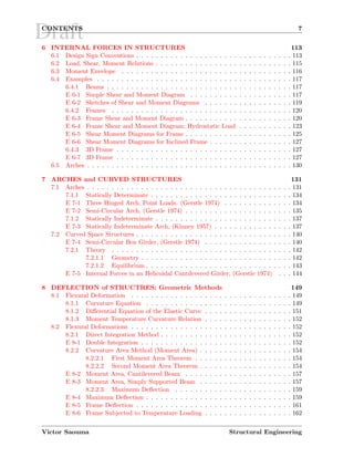
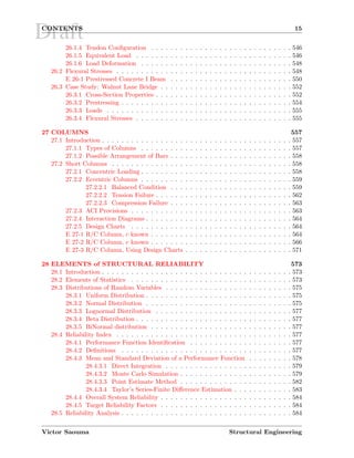
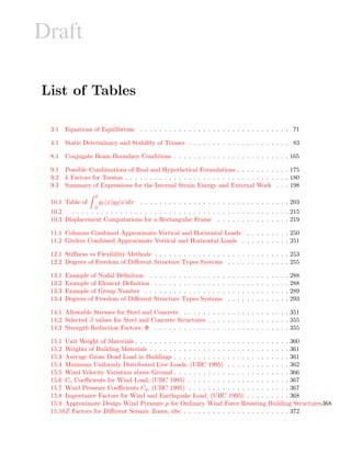
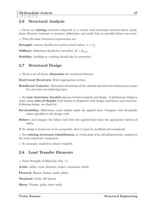
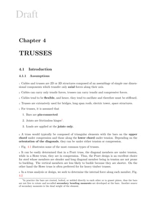
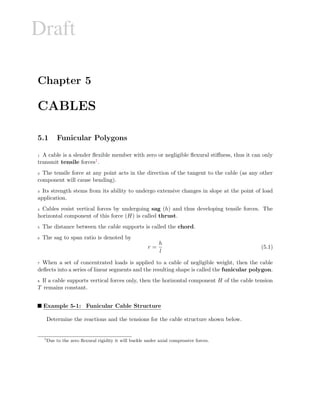
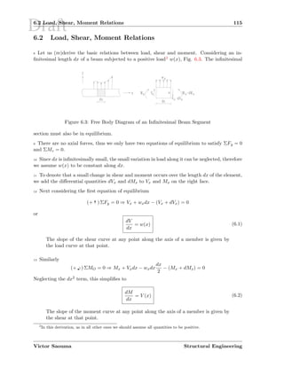
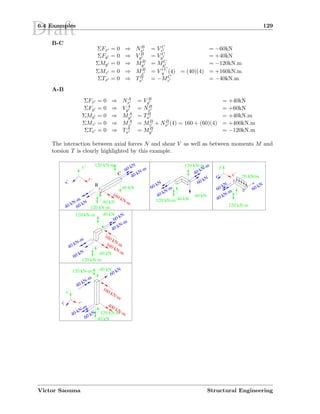
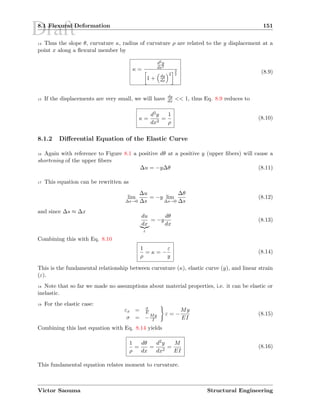
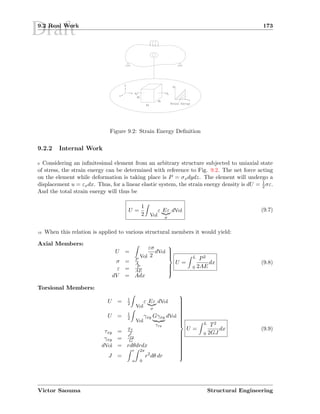
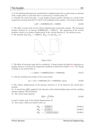
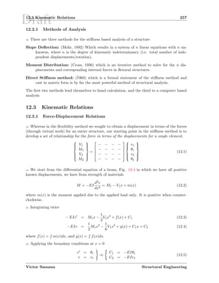
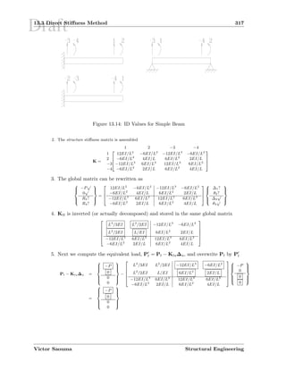
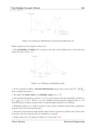
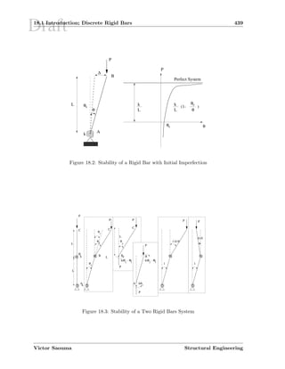
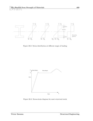
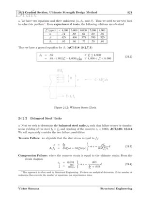
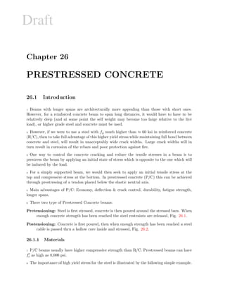
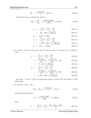
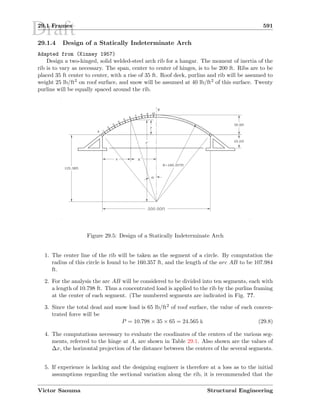
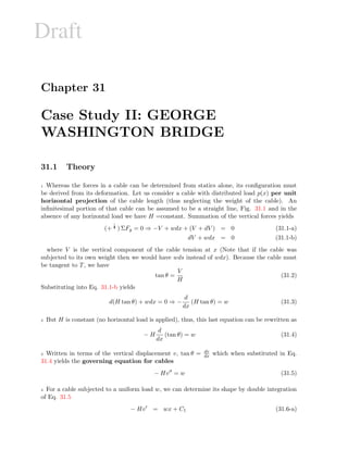
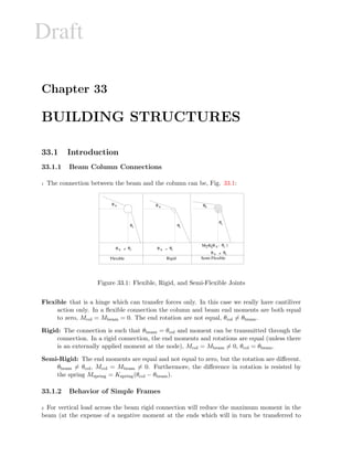
Example 7-2: Semi-Circular Arch, (Gerstle 1974)
Determine the reactions of the three hinged statically determined semi-circular arch under
its own dead weight w (per unit arc length s, where ds = rdθ). 7.6
R cosθ
R
A
B
C
R
A
B
θ
dP=wRdθ
θ
rθ
Figure 7.6: Semi-Circular three hinged arch
Solution:
I Reactions The reactions can be determined by integrating the load over the entire struc-
ture
1. Vertical Reaction is determined first:
(+ ¡') ΣMA = 0; −(Cy)(2R) +
θ=π
θ=0
wRdθ
dP
R(1 + cos θ)
moment arm
= 0 (7.6-a)
⇒ Cy =
wR
2
θ=π
θ=0
(1 + cos θ)dθ =
wR
2
[θ − sin θ] |θ=π
θ=0
=
wR
2
[(π − sin π) − (0 − sin 0)]
= π
2 wR (7.6-b)
2. Horizontal Reactions are determined next
(+
¡
') ΣMB = 0; −(Cx)(R) + (Cy)(R) −
θ= π
2
θ=0
wRdθ
dP
R cos θ
moment arm
= 0 (7.7-a)
Victor Saouma Structural Engineering](https://image.slidesharecdn.com/lecture-notes-in-structural-engineering-analysis-design-160511112755/85/Lecture-notes-in-structural-engineering-analysis-design-38-320.jpg)
![Draft10.3 Short-Cut for Displacement Evaluation 203
Note that D0
i is the vector of initial displacements, which is usually zero unless we have
an initial displacement of the support (such as support settlement).
7. The reactions are then obtained by simply inverting the flexibility matrix.
9 Note that from Maxwell-Betti’s reciprocal theorem, the flexibility matrix [f] is always sym-
metric.
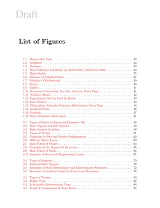
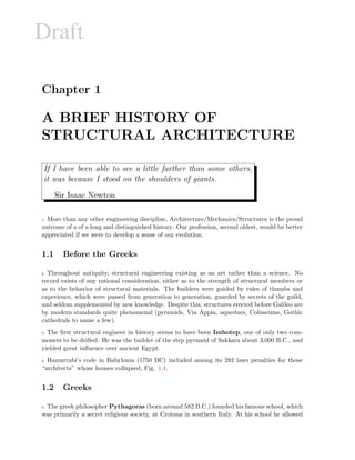
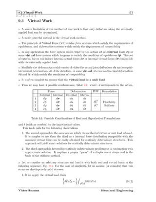
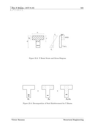
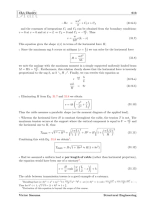
10.3 Short-Cut for Displacement Evaluation
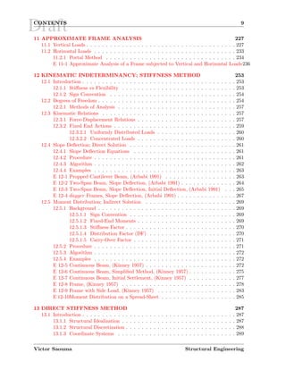
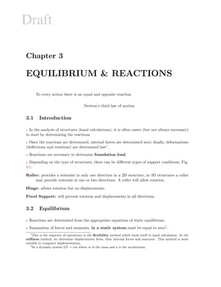
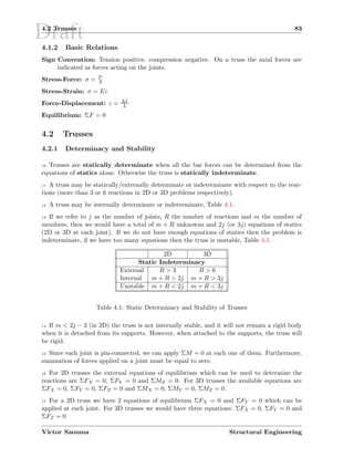
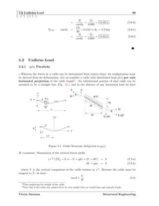
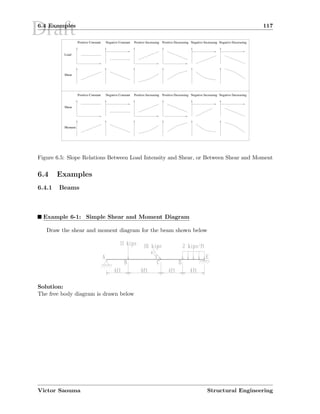
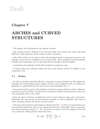
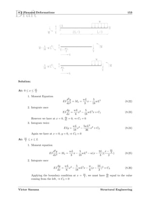
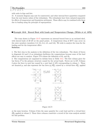
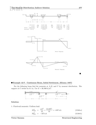
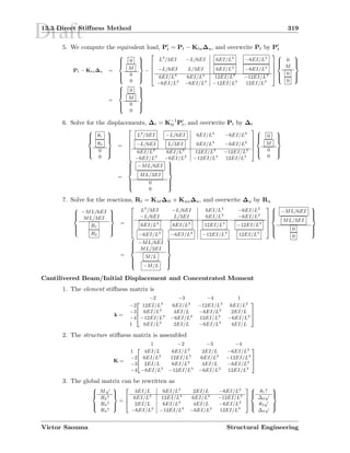
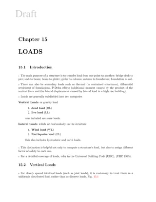
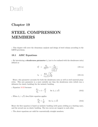
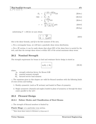
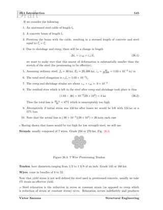
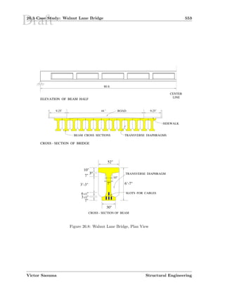
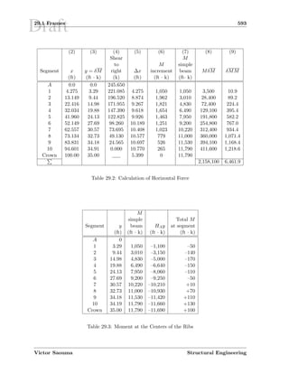
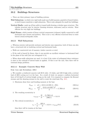
10 Since deflections due to flexural effects must be determined numerous times in the flexibility
method, Table 10.1 may simplify some of the evaluation of the internal strain energy. You are
strongly discouraged to use this table while still at school!.
g2(x)
g1(x) L
a
r
rr
L
a
222
L
a b
L
c
Lac Lac
2
Lc(a+b)
2
rrr
L
c
Lac
2
Lac
3
Lc(2a+b)
6
¨¨¨
L
c
Lac
2
Lac
6
Lc(a+2b)
6
222
L
c d
La(c+d)
2
La(2c+d)
6
La(2c+d)+Lb(c+2d)
6
L
c d e
La(c+4d+e)
6
La(c+2d)
6
La(c+2d)+Lb(2d+e)
6
Table 10.1: Table of
L
0
g1(x)g2(x)dx
10.4 Examples
Example 10-1: Steel Building Frame Analysis, (White et al. 1976)
A small, mass-produced industrial building, Fig. 10.3, is to be framed in structural steel
with a typical cross section as shown below. The engineer is considering three different designs
for the frame: (a) for poor or unknown soil conditions, the foundations for the frame may not
be able to develop any dependable horizontal forces at its bases. In this case the idealized
base conditions are a hinge at one of the bases and a roller at the other; (b) for excellent
Victor Saouma Structural Engineering](https://image.slidesharecdn.com/lecture-notes-in-structural-engineering-analysis-design-160511112755/85/Lecture-notes-in-structural-engineering-analysis-design-48-320.jpg)

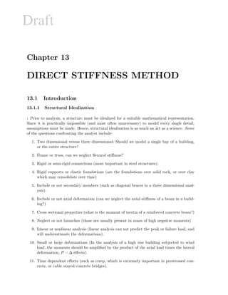
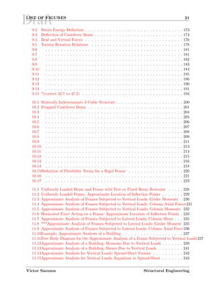
![Draft13.1 Introduction 293
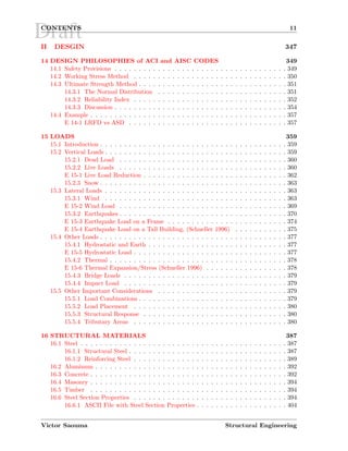
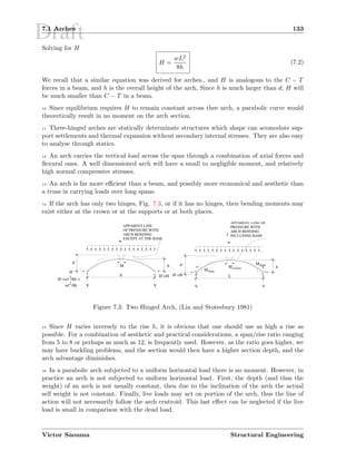
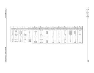
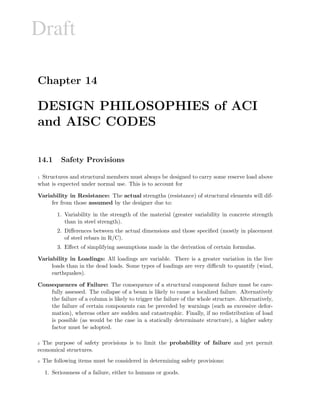
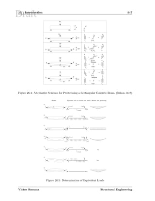
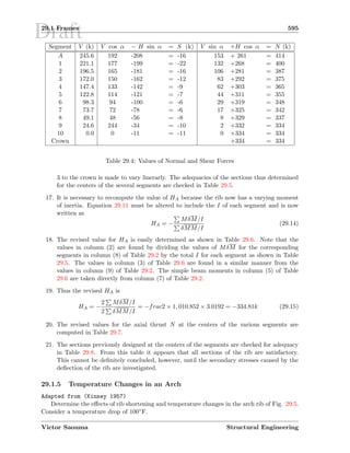
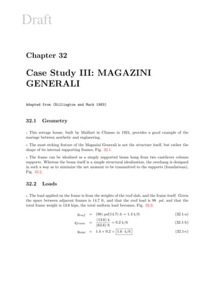
Type Node 1 Node 2 [k] [K]
(Local) (Global)
1 Dimensional
{p} Fy1, Mz2 Fy3, Mz4
Beam 4 × 4 4 × 4
{δ} v1, θ2 v3, θ4
2 Dimensional
{p} Fx1 Fx2
Truss 2 × 2 4 × 4
{δ} u1 u2
{p} Fx1, Fy2, Mz3 Fx4, Fy5, Mz6
Frame 6 × 6 6 × 6
{δ} u1, v2, θ3 u4, v5, θ6
{p} Tx1, Fy2, Mz3 Tx4, Fy5, Mz6
Grid 6 × 6 6 × 6
{δ} θ1, v2, θ3 θ4, v5, θ6
3 Dimensional
{p} Fx1, Fx2
Truss 2 × 2 6 × 6
{δ} u1, u2
{p} Fx1, Fy2, Fy3, Fx7, Fy8, Fy9,
Tx4 My5, Mz6 Tx10 My11, Mz12
Frame 12 × 12 12 × 12
{δ} u1, v2, w3, u7, v8, w9,
θ4, θ5 θ6 θ10, θ11 θ12
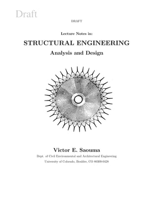
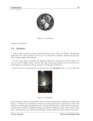
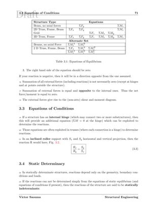
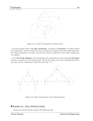
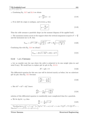
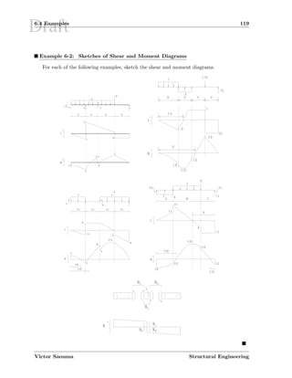
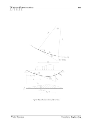
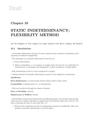
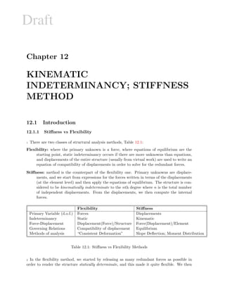
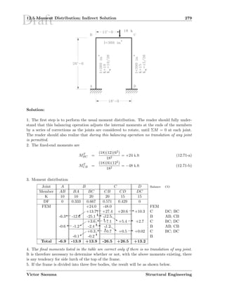
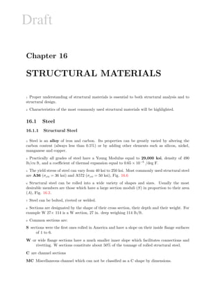
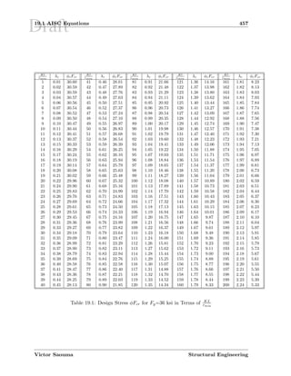
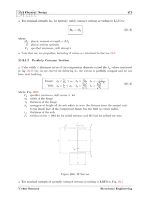
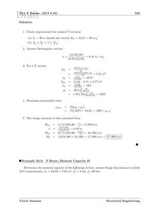
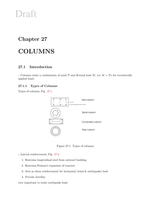
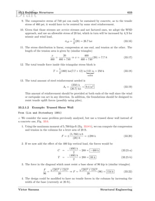
Table 13.4: Degrees of Freedom of Different Structure Types Systems
Victor Saouma Structural Engineering](https://image.slidesharecdn.com/lecture-notes-in-structural-engineering-analysis-design-160511112755/85/Lecture-notes-in-structural-engineering-analysis-design-69-320.jpg)
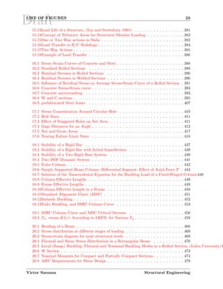
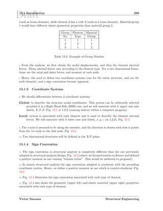
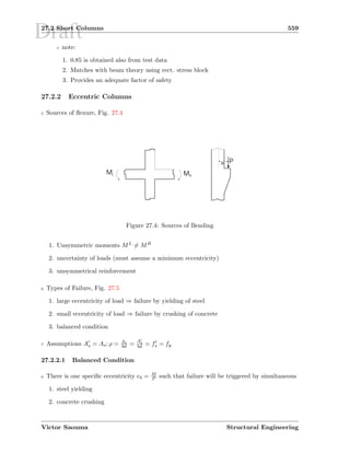
![Draft13.2 Stiffness Matrices 295
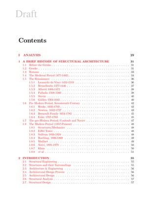
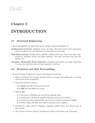
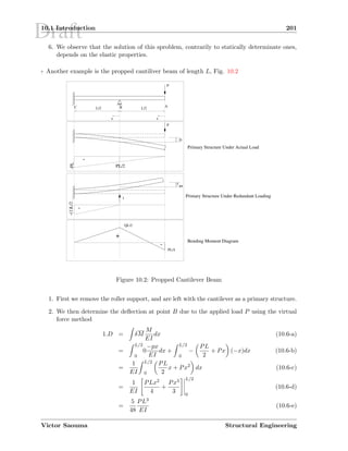
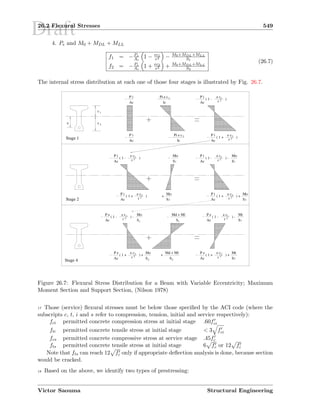
13.2 Stiffness Matrices
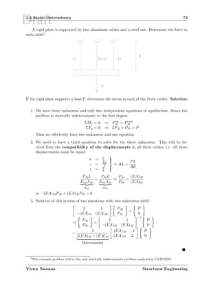
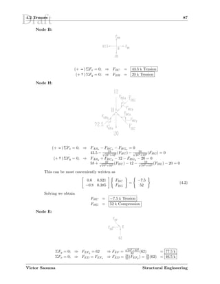
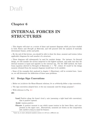
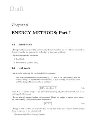
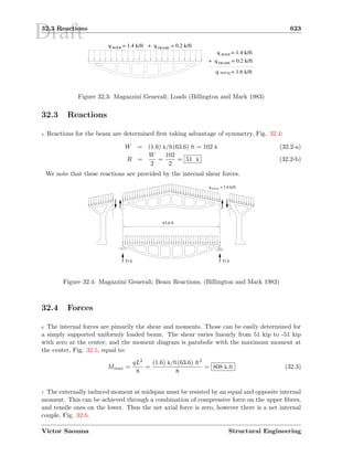
13.2.1 Truss Element
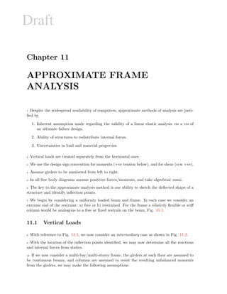
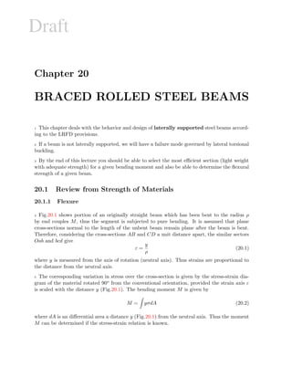
22 From strength of materials, the force/displacement relation in axial members is
σ = E
Aσ
P
=
AE
L
∆
1
(13.1)
Hence, for a unit displacement, the applied force should be equal to AE
L . From statics, the force
at the other end must be equal and opposite.
23 The truss element (whether in 2D or 3D) has only one degree of freedom associated with
each node. Hence, from Eq. 13.1, we have
[kt
] =
AE
L
u1 u2
p1 1 −1
p2 −1 1
(13.2)
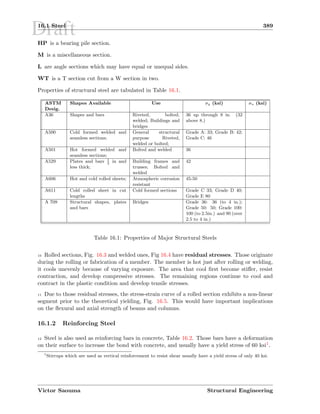
13.2.2 Beam Element
24 Using Equations 12.10, 12.10, 12.12 and 12.12 we can determine the forces associated with
each unit displacement.
[kb
] =
v1 θ1 v2 θ2
V1 Eq. 12.12(v1 = 1) Eq. 12.12(θ1 = 1) Eq. 12.12(v2 = 1) Eq. 12.12(θ2 = 1)
M1 Eq. 12.10(v1 = 1) Eq. 12.10(θ1 = 1) Eq. 12.10(v2 = 1) Eq. 12.10(θ2 = 1)
V2 Eq. 12.12(v1 = 1) Eq. 12.12(θ1 = 1) Eq. 12.12(v2 = 1) Eq. 12.12(θ2 = 1)
M2 Eq. 12.10(v1 = 1) Eq. 12.10(θ1 = 1) Eq. 12.10(v2 = 1) Eq. 12.10(θ2 = 1)
(13.3)
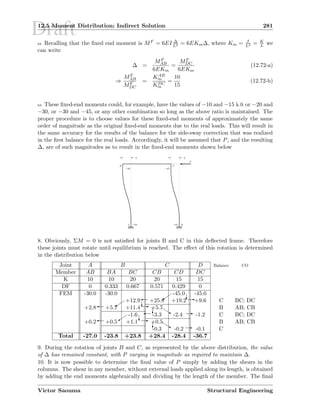
25 The stiffness matrix of the beam element (neglecting shear and axial deformation) will thus
be
[kb
] =
v1 θ1 v2 θ2
V1
12EIz
L3
6EIz
L2 −12EIz
L3
6EIz
L2
M1
6EIz
L2
4EIz
L −6EIz
L2
2EIz
L
V2 −12EIz
L3 −6EIz
L2
12EIz
L3 −6EIz
L2
M2
6EIz
L2
2EIz
L −6EIz
L2
4EIz
L
(13.4)
26 We note that this is identical to Eq.12.14
V1
M1
V2
M2
=
v1 θ1 v2 θ2
V1
12EIz
L3
6EIz
L2 −12EIz
L3
6EIz
L2
M1
6EIz
L2
4EIz
L −6EIz
L2
2EIz
L
V2 −12EIz
L3 −6EIz
L2
12EIz
L3 −6EIz
L2
M2
6EIz
L2
2EIz
L −6EIz
L2
4EIz
L
k(e)
v1
θ1
v2
θ2
(13.5)
Victor Saouma Structural Engineering](https://image.slidesharecdn.com/lecture-notes-in-structural-engineering-analysis-design-160511112755/85/Lecture-notes-in-structural-engineering-analysis-design-70-320.jpg)
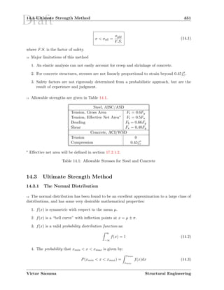
![Draft13.3 Direct Stiffness Method 315
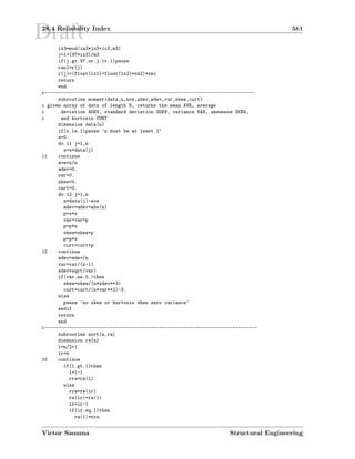
% Solve for the Displacements in meters and radians
Displacements=inv(Ktt)*P’
% Extract Kut
Kut=Kaug(4:9,1:3);
% Compute the Reactions and do not forget to add fixed end actions
Reactions=Kut*Displacements+FEA_Rest’
% Solve for the internal forces and do not forget to include the fixed end actions
dis_global(:,:,1)=[0,0,0,Displacements(1:3)’];
dis_global(:,:,2)=[Displacements(1:3)’,0,0,0];
for elem=1:2
dis_local=Gamma(:,:,elem)*dis_global(:,:,elem)’;
int_forces=k(:,:,elem)*dis_local+fea(1:6,elem)
end
function [k,K,Gamma]=stiff(EE,II,A,i,j)
% Determine the length
L=sqrt((j(2)-i(2))^2+(j(1)-i(1))^2);
% Compute the angle theta (carefull with vertical members!)
if(j(1)-i(1))~=0
alpha=atan((j(2)-i(2))/(j(1)-i(1)));
else
alpha=-pi/2;
end
% form rotation matrix Gamma
Gamma=[
cos(alpha) sin(alpha) 0 0 0 0;
-sin(alpha) cos(alpha) 0 0 0 0;
0 0 1 0 0 0;
0 0 0 cos(alpha) sin(alpha) 0;
0 0 0 -sin(alpha) cos(alpha) 0;
0 0 0 0 0 1];
% form element stiffness matrix in local coordinate system
EI=EE*II;
EA=EE*A;
k=[EA/L, 0, 0, -EA/L, 0, 0;
0, 12*EI/L^3, 6*EI/L^2, 0, -12*EI/L^3, 6*EI/L^2;
0, 6*EI/L^2, 4*EI/L, 0, -6*EI/L^2, 2*EI/L;
-EA/L, 0, 0, EA/L, 0, 0;
0, -12*EI/L^3, -6*EI/L^2, 0, 12*EI/L^3, -6*EI/L^2;
0, 6*EI/L^2, 2*EI/L, 0, -6*EI/L^2, 4*EI/L];
% Element stiffness matrix in global coordinate system
K=Gamma’*k*Gamma;
This simple proigram will produce the following results:
Displacements =
0.0010
-0.0050
Victor Saouma Structural Engineering](https://image.slidesharecdn.com/lecture-notes-in-structural-engineering-analysis-design-160511112755/85/Lecture-notes-in-structural-engineering-analysis-design-72-320.jpg)


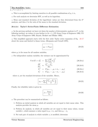
![Draft22.3 Examples 499
be developed or whether buckling behavior controls the bending behavior. The values for
Lp and Lr can be calculated using Eq. 6-1 and 6-2 respectively or they can be found in
the beam section of the LRFD manual. In either case these values for a W 12 × 120 are:
Lp = 13 ft
Lr = 75.5 ft
5. Since our unbraced length falls between these two values, the beam will be controlled
by inelastic buckling, and the nominal moment capacity Mn can be calculated from Eq.
6-5. Using this equation we must first calculate the plastic and elastic moment capacity
values, Mp and Mr.
Mp = FyZx = (36) ksi(186) in3 ft
(12) in = 558 k.ft
Mr = (Fyw − 10) ksiSx
(36 − 10) ksi(163) in3 = 353.2 k.ft
6. Using Eq. 6-5 (assuming Cb is equal to 1.0) we find:
Mn = Cb[Mp − (Mp − Mr)]
lb−Lp
Lr−Lp
Mn = 1.0[558 − (558 − 453.2)] k.ft
(15−13) ft
(75.5−15) ft
= 551.4 k.ft
7. Therefore the design moment capacity is as follows:
φbMn = 0.90(551.4) k.ft = 496.3 k.ft
8. Now consider the effects of moment magnification on this section. Based on the alternative
method and since the member is not subjected to sidesway (Mlt = 0)
Mu = B1Mnt
B1 = Cm
1− Pu
Pe
Cm = .60 − .4M1
M2
Cm = .60 − .4−50
50 = 1.0
Pu = 400 k
Pe =
π2EAg
Kl
r
2 (Euler’s Buckling Load Equation)
Pe = π2(29,000 ksi)(35.3 in2
)
32.672 = 9, 456 k
9. Therefore, calculating the B1 magnifier we find:
B1 =
1
1 − (400) k
(9,456) k
= 1.044
Calculating the amplified moment as follows:
Mu = B1Mnt
Mu = 1.044(50) k.ft = 52.2 k.ft
Therefore the adequacy of the section is calculated from Eq. as follows:
Pu
φcPn
+ 8
9
Mux
φbMnx ≤ 1.0
94000 k
(907.6) k + 8
9
(52.2) k.ft
(496.3) k.ft = .53 1.0
√
Victor Saouma Structural Engineering](https://image.slidesharecdn.com/lecture-notes-in-structural-engineering-analysis-design-160511112755/85/Lecture-notes-in-structural-engineering-analysis-design-102-320.jpg)

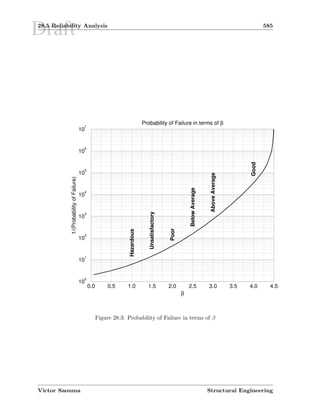
![Draft28.3 Distributions of Random Variables 575
Skewness: characterizes the degree of asymmetry of a distribution around its mean. It is
defined in a non-dimensional value. A positive one signifies a distribution with an asym-
metric tail extending out toward more positive x
Skew =
1
N
ΣN
i=1
xi − µ
σ
3
(28.8)
Kurtosis: is a nondimensional quantity which measures the “flatness” or “peakedness” of a
distribution. It is normalized with respect to the curvature of a normal distribution.
Hence a negative value would result from a distribution resembling a loaf of bread, while
a positive one would be induced by a sharp peak:
Kurt =
1
N
ΣN
i=1
xi − µ
σ
4
− 3 (28.9)
the −3 term makes the value zero for a normal distribution.
6 The expected value (or mean), standard deviation and coefficient of variation are interdepen-
dent: knowing any two, we can determine the third.
28.3 Distributions of Random Variables
7 Distribution of variables can be mathematically represented.
28.3.1 Uniform Distribution
8 Uniform distribution implies that any value between xmin and xmax is equaly likely to occur.
28.3.2 Normal Distribution
9 The general normal (or Gauss) distribution is given by, Fig. 28.1:
φ(x) =
1
√
2πσ
e− 1
2 [x−µ
σ ]
2
(28.10)
10 A normal distribution N(µ, σ2) can be normalized by defining
y =
x − µ
σ
(28.11)
and y would have a distribution N(0, 1):
φ(y) =
1
√
2π
e− y2
2 (28.12)
11 The normal distribution has been found to be an excellent approximation to a large class of
distributions, and has some very desirable mathematical properties:
Victor Saouma Structural Engineering](https://image.slidesharecdn.com/lecture-notes-in-structural-engineering-analysis-design-160511112755/85/Lecture-notes-in-structural-engineering-analysis-design-122-320.jpg)
![Draft28.4 Reliability Index 579
30 The objective is to determine the mean and standard deviation of the performance function
defined in terms of C/D.
31 Those two parameters, in turn, will later be required to compute the reliability index.
28.4.3.1 Direct Integration
32 Given a function random variable x, the mean value of the function is obtained by integrating
the function over the probability distribution function of the random variable
µ[F(x)] =
∞
−∞
g(x)f(x)dx (28.21)
33 For more than one variable,
µ[F(x)] =
∞
−∞
∞
−∞
· · ·
∞
−∞
F(x1, x2, · · · , xn)F(x1, x2, · · · , xn)dx1dx2 · · · dxn (28.22)
34 Note that in practice, the function F(x) is very rarely available for practical problems, and
hence this method is seldom used.
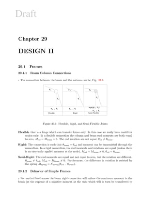
28.4.3.2 Monte Carlo Simulation
35 The performance function is evaluated for many possible values of the random variables.
36 Assuming that all variables have a normal distribution, then this is done through the following
algorithm
1. initialize random number generators
2. Perform n analysis, for each one:
(a) For each variable, determine a random number for the given distribution
(b) Transform the random number
(c) Analyse
(d) Determine the performance function, and store the results
3. From all the analyses, determine the mean and the standard deviation, compute the
reliability index.
4. Count the number of analyses, nf which performance function indicate failure, the likeli-
hood of structural failure will be p(f) = nf /n.
37 A sample program (all subroutines are taken from (Press, Flannery, Teukolvsky and Vetterling
1988) which generates n normally distributed data points, and then analyze the results, deter-
mines mean and standard deviation, and sort them (for histogram plotting), is shown below:
program nice
parameter(ns=100000)
real x(ns), mean, sd
write(*,*)’enter mean, standard-deviation and n ’
read(*,*)mean,sd,n
Victor Saouma Structural Engineering](https://image.slidesharecdn.com/lecture-notes-in-structural-engineering-analysis-design-160511112755/85/Lecture-notes-in-structural-engineering-analysis-design-124-320.jpg)


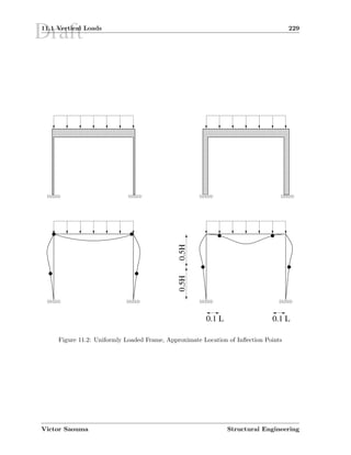
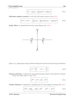
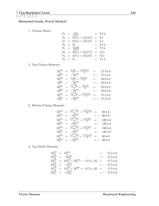
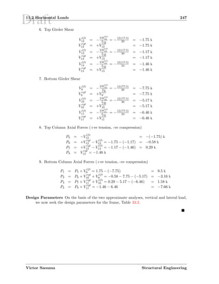
The document is a preface for a textbook on structural engineering. It aims to provide a succinct yet rigorous coverage of structural analysis and design by combining these topics. It uses an unusual format that clearly distinguishes key ideas to foster learning. All example problems have been carefully selected and typeset to enhance understanding. The preface explains that the textbook format aims to address the need for a single reference on structural engineering that combines analysis and design through numerous well-presented example problems.