Prof. Dr.-Ing. DietmarGross
received his Engineering Diploma in Applied Mechanics
and his Doctor of Engineering degree at the University of
Rostock. He was Research Associate at the University of
Stuttgart and since 1976 he is Professor of Mechanics at the
University of Darmstadt. His research interests are mainly
focused on modern solid mechanics on the macro and
micro scale, including advanced materials
Prof. Dr. Werner Hauger
studied Applied Mathematics and Mechanics at the
University of Karlsruhe and received his Ph.D. in Theoretical
and Applied Mechanics from Northwestern University in
Evanston. He worked in industry for several years, was a
Professor at the Helmut-Schmidt-University in Hamburg and
went to the University of Darmstadt in 1978. His research
interests are, among others, theory of stability, dynamic
plasticity and biomechanics.
Prof. Dr.-Ing. Jörg Schröder
studied Civil Engineering, received his doctoral degree at
the University of Hannover and habilitated at the University
of Stuttgart. He was Professor of Mechanics at the
University of Darmstadt and went to the University of
Duisburg-Essen in 2001. His fields of research are
theoretical and computer-oriented continuum mechanics,
modeling of functional materials as well as the further
development of the finite element method.
Prof. Dr.-Ing. Wolfgang A. Wall
studied Civil Engineering at Innsbruck University and
received his doctoral degree from the University of Stuttgart.
Since 2003 he is Professor of Mechanics at the TU München
and Head of the Institute for Computational Mechanics. His
research interests cover broad fields in computational
mechanics, including both solid and fluid mechanics. His
recent focus is on multiphysics and multiscale problems as
well as computational biomechanics.
Prof. Nimal Rajapakse
studied Civil Engineering at the University of Sri Lanka and
received Doctor of Engineering from the Asian Institute of
Technology in 1983. He was Professor of Mechanics and
Department Head at the University of Manitoba and at the
University of British Columbia. He is currently Dean of
Applied Sciences at Simon Fraser University in Vancouver.
His research interests include mechanics of advanced
materials and geomechanics.
4.
Dietmar Gross •Werner Hauger
Jörg Schröder • Wolfgang A. Wall
Nimal Rajapakse
Engineering Mechanics 1
Statics
2nd Edition
123
Preface
Statics is thefirst volume of a three-volume textbook on Engi-
neering Mechanics. Volume 2 deals with Mechanics of Materials;
Volume 3 contains Particle Dynamics and Rigid Body Dynamics.
The original German version of this series is the bestselling text-
book on mechanics for nearly three decades and its 11th edition
has already been published.
It is our intention to present to engineering students the basic
concepts and principles of mechanics in the clearest and simp-
lest form possible. A major objective of this book is to help the
students to develop problem solving skills in a systematic manner.
The book developed out of many years of teaching experience
gained by the authors while giving courses on engineering me-
chanics to students of mechanical, civil and electrical engineering.
The contents of the book correspond to the topics normally co-
vered in courses on basic engineering mechanics at universities
and colleges. The theory is presented in as simple a form as the
subject allows without being imprecise. This approach makes the
text accessible to students from different disciplines and allows for
their different educational backgrounds. Another aim of the book
is to provide students as well as practising engineers with a solid
foundation to help them bridge the gaps between undergraduate
studies, advanced courses on mechanics and practical engineering
problems.
A thorough understanding of the theory cannot be acquired
by merely studying textbooks. The application of the seemingly
simple theory to actual engineering problems can be mastered
only if the student takes an active part in solving the numerous
examples in this book. It is recommended that the reader tries to
solve the problems independently without resorting to the given
solutions. To demonstrate the principal way of how to apply the
theory we deliberately placed no emphasis on numerical solutions
and numerical results.
7.
VI
As a specialfeature the textbook offers the TM-Tools. Students
may solve various problems of mechanics using these tools. They
can be found at the web address <www.springer.com/engineering/
grundlagen/tm-tools>.
In the second edition the text was revised and part of the nota-
tion was changed to make it compatible with the usual notation
in English speaking countries. To provide the students with mo-
re material to develop their skills in solving problems, additional
Supplementary Examples are supplied.
We gratefully acknowledge the support and the cooperation of
the staff of Springer who were responsive to our wishes and helped
to create the present layout of the books.
Darmstadt, Essen, Munich and Vancouver, D. Gross
Summer 2012 W. Hauger
J. Schröder
W.A. Wall
N. Rajapakse
8.
Table of Contents
Introduction...............................................................1
1 Basic Concepts
1.1 Force .............................................................. 7
1.2 Characteristics and Representation of a Force ............ 7
1.3 The Rigid Body ................................................. 9
1.4 Classification of Forces, Free-Body Diagram .............. 10
1.5 Law of Action and Reaction .................................. 13
1.6 Dimensions and Units.......................................... 14
1.7 Solution of Statics Problems, Accuracy .................... 16
1.8 Summary ......................................................... 18
2 Forces with a Common Point of Application
2.1 Addition of Forces in a Plane................................. 21
2.2 Decomposition of Forces in a Plane, Representation in
Cartesian Coordinates.......................................... 25
2.3 Equilibrium in a Plane ......................................... 29
2.4 Examples of Coplanar Systems of Forces................... 30
2.5 Concurrent Systems of Forces in Space .................... 38
2.6 Supplementary Problems ...................................... 44
2.7 Summary ......................................................... 49
3 General Systems of Forces, Equilibrium of a Rigid Body
3.1 General Systems of Forces in a Plane....................... 53
3.1.1 Couple and Moment of a Couple ............................ 53
3.1.2 Moment of a Force ............................................. 57
3.1.3 Resultant of Systems of Coplanar Forces .................. 59
3.1.4 Equilibrium Conditions......................................... 62
3.2 General Systems of Forces in Space......................... 71
3.2.1 The Moment Vector............................................ 71
3.2.2 Equilibrium Conditions......................................... 77
3.3 Supplementary Problems ...................................... 83
3.4 Summary ......................................................... 88
4 Center of Gravity, Center of Mass, Centroids
4.1 Center of Forces................................................. 91
9.
VIII
4.2 Center ofGravity and Center of Mass ...................... 94
4.3 Centroid of an Area ............................................ 100
4.4 Centroid of a Line .............................................. 110
4.5 Supplementary Problems ...................................... 112
4.6 Summary ......................................................... 116
5 Support Reactions
5.1 Plane Structures ................................................ 119
5.1.1 Supports .......................................................... 119
5.1.2 Statical Determinacy ........................................... 122
5.1.3 Determination of the Support Reactions ................... 125
5.2 Spatial Structures............................................... 127
5.3 Multi-Part Structures .......................................... 130
5.3.1 Statical Determinacy ........................................... 130
5.3.2 Three-Hinged Arch ............................................. 136
5.3.3 Hinged Beam .................................................... 139
5.3.4 Kinematical Determinacy...................................... 142
5.4 Supplementary Problems ...................................... 145
5.5 Summary ......................................................... 150
6 Trusses
6.1 Statically Determinate Trusses ............................... 153
6.2 Design of a Truss ............................................... 155
6.3 Determination of the Internal Forces........................ 158
6.3.1 Method of Joints................................................ 158
6.3.2 Method of Sections............................................. 163
6.4 Supplementary Problems ...................................... 167
6.5 Summary ......................................................... 171
7 Beams, Frames, Arches
7.1 Stress Resultants................................................ 175
7.2 Stress Resultants in Straight Beams ....................... 180
7.2.1 Beams under Concentrated Loads ........................... 180
7.2.2 Relationship between Loading
and Stress Resultants .......................................... 188
7.2.3 Integration and Boundary Conditions ....................... 190
7.2.4 Matching Conditions ........................................... 195
10.
IX
7.2.5 Pointwise Constructionof the Diagrams ................... 200
7.3 Stress Resultants in Frames and Arches.................... 205
7.4 Stress Resultants in Spatial Structures ..................... 211
7.5 Supplementary Problems ...................................... 215
7.6 Summary ......................................................... 220
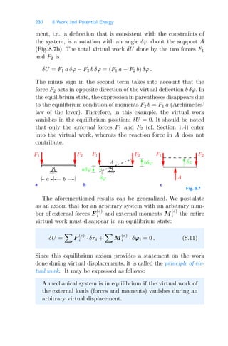
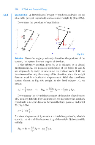
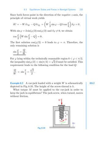
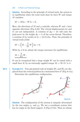
8 Work and Potential Energy
8.1 Work and Potential Energy ................................... 223
8.2 Principle of Virtual Work...................................... 229
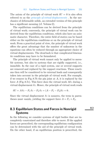
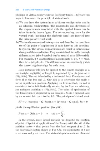
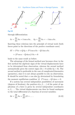
8.3 Equilibrium States and Forces in Nonrigid Systems ...... 231
8.4 Reaction Forces and Stress Resultants...................... 237
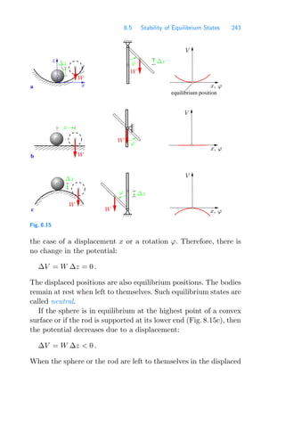
8.5 Stability of Equilibrium States................................ 242
8.6 Supplementary Problems ...................................... 253
8.7 Summary ......................................................... 258
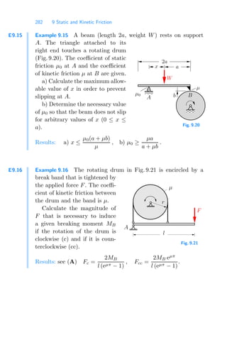
9 Static and Kinetic Friction
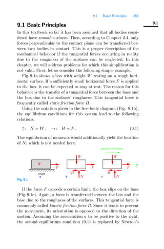
9.1 Basic Principles ................................................. 261
9.2 Coulomb Theory of Friction .................................. 263
9.3 Belt Friction ..................................................... 273
9.4 Supplementary Problems ...................................... 278
9.5 Summary ......................................................... 283
A Vectors, Systems of Equations
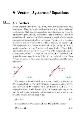
A.1 Vectors............................................................ 286
A.1.1 Multiplication of a Vector by a Scalar ...................... 289
A.1.2 Addition and Subtraction of Vectors........................ 289
A.1.3 Dot Product ..................................................... 290
A.1.4 Vector Product (Cross-Product) ............................. 291
A.2 Systems of Linear Equations.................................. 293
Index ........................................................................ 299
11.
Introduction
Mechanics is theoldest and the most highly developed branch
of physics. As important foundation of engineering, its relevance
continues to increase as its range of application grows.
The tasks of mechanics include the description and determi-
nation of the motion of bodies, as well as the investigation of the
forces associated with the motion. Technical examples of such mo-
tions are the rolling wheel of a vehicle, the flow of a fluid in a duct,
the flight of an airplane and the orbit of a satellite. “Motion” in
a generalized sense includes the deflection of a bridge or the de-
formation of a structural element under the influence of a load.
An important special case is the state of rest; a building, dam or
television tower should be constructed in such a way that it does
not move or collapse.
Mechanics is based on only a few laws of nature which have
an axiomatic character. These are statements based on numerous
observations and regarded as being known from experience. The
conclusions drawn from these laws are also confirmed by experi-
ence. Mechanical quantities such as velocity, mass, force, momen-
tum or energy describing the mechanical properties of a system are
connected within these axioms and within the resulting theorems.
Real bodies or real technical systems with their multifaceted
properties are neither considered in the basic principles nor in
their applications to technical problems. Instead, models are in-
vestigated that possess the essential mechanical characteristics of
the real bodies or systems. Examples of these idealisations are a
rigid body or a mass point. Of course, a real body or a structural
element is always deformable to a certain extent. However, they
may be considered as being rigid bodies if the deformation does not
play an essential role in the behaviour of the mechanical system.
To investigate the path of a stone thrown by hand or the orbit of
a planet in the solar system, it is usually sufficient to view these
bodies as being mass points, since their dimensions are very small
compared with the distances covered.
In mechanics we use mathematics as an exact language. Only
mathematics enables precise formulation without reference to a
12.
2 Introduction
certain placeor a certain time and allows to describe and compre-
hend mechanical processes. If an engineer wants to solve a tech-
nical problem with the aid of mechanics he or she has to replace
the real technical system with a model that can be analysed ma-
thematically by applying the basic mechanical laws. Finally, the
mathematical solution has to be interpreted mechanically and eva-
luated technically.
Since it is essential to learn and understand the basic princip-
les and their correct application from the beginning, the question
of modelling will be mostly omitted in this text, since it requi-
res a high degree of competence and experience. The mechanical
analysis of an idealised system in which the real technical system
may not always be easily recognised is, however, not simply an
unrealistic game. It will familiarise students with the principles
of mechanics and thus enable them to solve practical engineering
problems independently.
Mechanics may be classified according to various criteria. De-
pending on the state of the material under consideration, one
speaks of the mechanics of solids, hydrodynamics or gasdynamics.
In this text we will consider solid bodies only, which can be clas-
sified as rigid, elastic or plastic bodies. In the case of a liquid one
distinguishes between a frictionless and a viscous liquid. Again,
the characteristics rigid, elastic or viscous are idealisations that
make the essential properties of the real material accessible to
mathematical treatment.
According to the main task of mechanics, namely, the investi-
gation of the state of rest or motion under the action of forces, me-
chanics may be divided into statics and dynamics. Statics (Latin:
status = standing) deals with the equilibrium of bodies subjected
to forces. Dynamics (Greek: dynamis = force) is subdivided into
kinematics and kinetics. Kinematics (Greek: kinesis = movement)
investigates the motion of bodies without referring to forces as a
cause or result of the motion. This means that it deals with the
geometry of the motion in time and space, whereas kinetics relates
the forces involved and the motion.
Alternatively, mechanics may be divided into analytical mecha-
nics and engineering mechanics. In analytical mechanics, the ana-
13.
Introduction 3
lytical methodsof mathematics are applied with the aim of gaining
principal insight into the laws of mechanics. Here, details of the
problems are of no particular interest. Engineering mechanics con-
centrates on the needs of the practising engineer. The engineer has
to analyse bridges, cranes, buildings, machines, vehicles or com-
ponents of microsystems to determine whether they are able to
sustain certain loads or perform certain movements.
The historical origin of mechanics can be traced to ancient
Greece, although of course mechanical insight derived from expe-
rience had been applied to tools and devices much earlier. Several
cornerstones on statics were laid by the works of Archimedes (287–
212): lever and fulcrum, block and tackle, center of gravity and
buoyancy. Nothing more of great importance was discovered until
the time of the Renaissance. Further progress was then made by
Leonardo da Vinci (1452–1519) with his observations of the equi-
librium on an inclined plane, and by Simon Stevin (1548–1620)
with his discovery of the law of the composition of forces. The
first investigations on dynamics can be traced back to Galileo Ga-
lilei (1564–1642) who discovered the law of gravitation. The laws
of planetary motion by Johannes Kepler (1571–1630) and the nu-
merous works of Christian Huygens (1629–1695) finally led to the
formulation of the laws of motion by Isaac Newton (1643–1727).
At this point, tremendous advancement was initiated, which went
hand in hand with the development of analysis and is associated
with the Bernoulli family (17th and 18th century), Leonhard Eu-
ler (1707–1783), Jean le Rond d’Alembert (1717–1783) and Joseph
Louis Lagrange (1736–1813). As a result of the progress made in
analytical and numerical methods – the latter especially boosted
by computer technology – mechanics today continues to enlarge
its field of application and makes more complex problems accessi-
ble to exact analysis. Mechanics also has its place in branches of
sciences such as medicine, biology and the social sciences through
the application of modelling and mathematical analysis.
1 Basic Concepts
1.1Force .............................................................. 7
1.2 Characteristics and Representation of a Force ........... 7
1.3 The Rigid Body................................................. 9
1.4 Classification of Forces, Free-Body Diagram ............. 10
1.5 Law of Action and Reaction ................................. 13
1.6 Dimensions and Units ......................................... 14
1.7 Solution of Statics Problems, Accuracy ................... 16
1.8 Summary ......................................................... 18
Objectives: Statics is the study of forces acting on bo-
dies that are in equilibrium. To investigate statics problems, it
is necessary to be familiar with some basic terms, formulas, and
work principles. Of particular importance are the method of secti-
ons, the law of action and reaction, and the free-body diagram, as
they are used to solve nearly all problems in statics.
16.
1.1 Force 7
1.1
1.1Force
The concept of force can be taken from our daily experience. Al-
though forces cannot be seen or directly observed, we are familiar
with their effects. For example, a helical spring stretches when
a weight is hung on it or when it is pulled. Our muscle tension
conveys a qualitative feeling of the force in the spring. Similarly,
a stone is accelerated by gravitational force during free fall, or
by muscle force when it is thrown. Also, we feel the pressure of
a body on our hand when we lift it. Assuming that gravity and
its effects are known to us from experience, we can characterize a
force as a quantity that is comparable to gravity.
In statics, bodies at rest are investigated. From experience we
know that a body subject only to the effect of gravity, falls. To
prevent a stone from falling, to keep it in equilibrium, we need to
exert a force on it, for example our muscle force. In other words:
A force is a physical quantity that can be brought into equi-
librium with gravity.
1.2
1.2 Characteristics and Representation of a Force
A single force is characterized by three properties: magnitude,
direction, and point of application.
The quantitative effect of a force is given by its magnitude.
A qualitative feeling for the magnitude is conveyed by different
muscle tensions when we lift different bodies or when we press
against a wall with varying intensities. The magnitude F of a force
can be measured by comparing it with gravity, i.e., with calibrated
or standardized weights. If the body of weight W in Fig. 1.1 is
in equilibrium, then F = W. The “Newton”, abbreviated N (cf.
Section 1.6), is used as the unit of force.
From experience we also know that force has a direction. While
gravity always has an effect downwards (towards the earth’s cen-
ter), we can press against a tabletop in a perpendicular or in an
inclined manner. The box on the smooth surface in Fig. 1.2 will
17.
8 1 BasicConcepts
0000
1111
W
α
f
F
Fig. 1.1
move in different directions, depending on the direction of the
force exerted upon it. The direction of the force can be described
by its line of action and its sense of direction (orientation). In
Fig. 1.1, the line of action f of the force F is inclined under the
angle α to the horizontal. The sense of direction is indicated by
the arrow.
Finally, a single force acts at a certain point of application. De-
pending on the location of point A in Fig. 1.2, the force will cause
different movements of the box.
A
A
F
F
A
F
A F
Fig. 1.2
A quantity determined by magnitude and direction is called a
vector. In contrast to a free vector, which can be moved arbitrarily
in space provided it maintains its direction, a force is tied to its line
of action and has a point of application. Therefore, we conclude:
The force is a bound vector.
According to standard vector notation, a force is denoted by a
boldfaced letter, for example by F , and its magnitude by |F | or
simply by F. In figures, a force is represented by an arrow, as
shown in Figs. 1.1 and 1.2. Since the vector character usually is
uniquely determined through the arrow, it is usually sufficient to
write only the magnitude F of the force next to the arrow.
In Cartesian coordinates (see Fig. 1.3 and Appendix A.1), the
force vector can be represented using the unit vectors ex, ey, ez
18.
1.3 The RigidBody 9
Fig. 1.3
y
F z
γ
β
z
x
F
F x
F y
ey
ex
α
ez
by
F = F x + F y + F z = Fx ex + Fy ey + Fz ez . (1.1)
Applying Pythagoras’ theorem in space, the force vector’s magni-
tude F is given by
F =
F2
x + F2
y + F2
z . (1.2)
The direction angles and therefore the direction of the force follow
from
cos α =
Fx
F
, cos β =
Fy
F
, cos γ =
Fz
F
. (1.3)
1.3
1.3 The Rigid Body
A body is called a rigid body if it does not deform under the influ-
ence of forces; the distances between different points of the body
remain constant. This is, of course, an idealization of a real bo-
dy composed of a reasonably stiff material which in many cases
is fulfilled in a good approximation. From experience with such
bodies it is known that a single force may be applied at any point
on the line of action without changing its effect on the body as a
whole (principle of transmissibility).
This principle is illustrated in Fig. 1.4. In the case of a de-
formable sphere, the effect of the force depends on the point of
19.
10 1 BasicConcepts
deformable
body
F
F
F
F
rigid body
f
f f
f
A1 A2
A2
A1
Fig. 1.4
application. In contrast, for a rigid sphere the effect of the force
F on the entire body is the same, regardless of whether the body
is pulled or pushed. In other words:
The effect of a force on a rigid body is independent of the
location of the point of application on the line of action. The
forces acting on rigid bodies are “sliding vectors”: they can
arbitrarily be moved along their action lines.
A parallel displacement of forces changes their effect considera-
bly. As experience shows, a body with weight W can be held in
equilibrium if it is supported appropriately (underneath the center
of gravity) by the force F, where F = W (Fig. 1.5a). Displacing
force F in a parallel manner causes the body to rotate (Fig. 1.5b).
a b
W
F
W
f
F
f
Fig. 1.5
1.4
1.4 Classification of Forces, Free-Body Diagram
A single force with a line of action and a point of application,
called a concentrated force, is an idealization that in reality does
not exist. It is almost realized when a body is loaded over a thin
wire or a needlepoint. In nature, only two kinds of forces exist:
volume forces and surface or area forces.
20.
1.4 Classification ofForces, Free-Body Diagram 11
A volume force is a force that is distributed over the volume of
a body or a portion thereof. Weight is an example of a volume
force. Every small particle (infinitesimal volume element dV ) of
the entire volume has a certain small (infinitesimal) weight dW
(Fig. 1.6a). The sum of the force elements dW, which are conti-
nuously distributed within the volume yields the total weight W.
Other examples of volume forces include magnetic and electrical
forces.
Area forces occur in the regions where two bodies are in con-
tact. Examples of forces distributed over an area include the water
pressure p at a dam (Fig. 1.6b), the snow load on a roof or the
pressure of a body on a hand.
A further idealization used in mechanics is the line force, which
comprises forces that are continuously distributed along a line. If
a blade is pressed against an object and the finite thickness of
the blade is disregarded, the line force q will act along the line of
contact (Fig. 1.6c).
0000000
0000000
1111111
1111111
b c
a
dW
dV
p
q
Fig. 1.6
Forces can also be classified according to other criteria. Active
forces refer to the physically prescribed forces in a mechanical
system, as for example the weight, the pressure of the wind or the
snow load on a roof.
Reaction forces are generated if the freedom of movement of
a body is constrained. For example, a falling stone is subjected
only to an active force due to gravity, i.e., its weight. However,
when the stone is held in the hand, its freedom of movement is
constrained; the hand exerts a reaction force on the stone.
Reaction forces can be visualized only if the body is separated
from its geometrical constraints. This procedure is called freeing
or cutting free or isolating the body. In Fig. 1.7a, a beam is loaded
21.
12 1 BasicConcepts
by an active force W. Supports A and B prevent the beam from
moving: they act on it through reaction forces that, for simplici-
ty, are also denoted by A and B. These reaction forces are made
visible in the so-called free-body diagram (Fig. 1.7b). It shows the
forces acting on the body instead of the geometrical constraints
through the supports. By this “freeing”, the relevant forces beco-
me accessible to analysis (cf. Chapter 5). This procedure is still
valid when a mechanical system becomes movable (dynamic) due
to freeing. In this case, the system is regarded as being frozen
when the reaction forces are determined. This is known as the
principle of solidification (cf. Section 5.3).
a b
free−body diagram
system
W W
A B
B
A
Fig. 1.7
A further classification is introduced by distinguishing between
external forces and internal forces. An external force acts from the
outside on a mechanical system. Active forces as well as reaction
forces are external forces. Internal forces act between the parts of
a system. They also can be visualized only by imaginary cutting or
sectioning of the body. If the body in Fig. 1.8a is sectioned by an
imaginary cut, the internal area forces p distributed over the cross-
section must be included in the free-body diagram; they replace
the initially perfect bonding between the two exposed surfaces
(Fig. 1.8b). This procedure is based on the hypothesis, which is
confirmed by experience, that the laws of mechanics are equally
valid for parts of the system. Accordingly, the system initially
consists of the complete body at rest. After the cut, the system
consists of two parts that act on each other through area forces in
such a way that each part is in equilibrium. This procedure, which
enables calculation of the internal forces, is called the method of
sections. It is valid for systems in equilibrium as well as for systems
in motion.
22.
1.5 Law ofAction and Reaction 13
a b
cut
p
W
A
p
B
W
A B
1 2
Fig. 1.8
Whether a force is an external or an internal force depends on
the system to be investigated. If the entire body in Fig. 1.8a is
considered to be the system, then the forces that become exposed
by the cut are internal forces: they act between the parts of the
system. On the other hand, if only part or only part of the
body in Fig. 1.8b is considered to be the system, the corresponding
forces are external forces.
As stated in Section 1.3, a force acting on a rigid body can be
displaced along its line of action without changing its effect on the
body. Consequently, the principle of transmissibility can be used
in the analysis of the external forces. However, this principle can
generally not be applied to internal forces. In this case, the body
is sectioned by imaginary cuts, therefore it matters whether an
external force acts on one or the other part.
The importance of internal forces in engineering sciences is de-
rived from the fact that their magnitude is a measure of the stress
in the material.
1.5
1.5 Law of Action and Reaction
A universally accepted law, based on everyday experience, is the
law of action and reaction. This axiom states that a force always
has a counteracting force of the same magnitude but of opposite
direction. Therefore, a force can never exist alone. If a hand is pres-
sed against a wall, the hand exerts a force F on the wall (Fig. 1.9a).
An opposite force of the same magnitude acts from the wall on
the hand. These forces can be made visible if the two bodies are
separated at the area of contact. Note that the forces act upon
23.
14 1 BasicConcepts
two different bodies. Analogously, a body on earth has a certain
weight W due to gravity. However, the body acts upon the earth
a b
000000000
000000000
000000000
000000000
000000000
000000000
000000000
000000000
000000000
000000000
111111111
111111111
111111111
111111111
111111111
111111111
111111111
111111111
111111111
111111111
0000
0000
0000
0000
0000
0000
0000
0000
0000
0000
0000
1111
1111
1111
1111
1111
1111
1111
1111
1111
1111
1111 cut
W
W
F F
Fig. 1.9
with a force of equal magnitude: they attract each other (Fig. 1.9b).
In short:
The forces that two bodies exert upon each other are of the
same magnitude but of opposite directions and they lie on
the same line of action.
This principle, which Newton succinctly expressed in Latin as
actio = reactio
is the third of Newton’s axioms (cf. Volume 3). It is valid for long-
range forces as well as for short-range forces, and it is independent
of whether the bodies are at rest or in motion.
1.6
1.6 Dimensions and Units
In mechanics the three basic physical quantities length, time and
mass are considered. Force is another important element that is
considered; however, from a physical point of view, force is a deri-
ved quantity. All other mechanical quantities, such as velocity, mo-
mentum or energy can be expressed by these four quantities. The
geometrical space where mechanical processes take place is three-
dimensional. However, as a simplification the discussion is limited
sometimes to two-dimensional or, in some cases, one-dimensional
problems.
24.
1.6 Dimensions andUnits 15
Associated with length, time, mass and force are their dimen-
sions [l], [t], [M] and [F]. According to the international SI unit
system (Système International d
Unités), they are expressed using
the base units meter (m), second (s) and kilogram (kg) and the
derived unit newton (N). A force of 1 N gives a mass of 1 kg the
acceleration of 1 m/s2
: 1 N = 1 kg m/s2
. Volume forces have the di-
mension force per volume [F/l3
] and are measured, for example,
as a multiple of the unit N/m3
. Similarly, area and line forces
have the dimensions [F/l2
] and [F/l] and the units N/m2
and
N/m, respectively.
The magnitude of a physical quantity is completely expres-
sed by a number and the unit. The notations F = 17 N or l =
3 m represent a force of 17 newtons or a distance of 3 meters,
respectively. In numerical calculations units are treated in the
same way as numbers. For example, using the above quantities,
F · l = 17 N · 3 m = 17 · 3 Nm = 51 Nm. In physical equations,
each side and each additive term must have the same dimension.
This should always be kept in mind when equations are formulated
or checked.
Very large or very small quantities are generally expressed by
attaching prefixes to the units meter, second, newton, and so forth:
k (kilo = 103
), M (mega = 106
), G (giga = 109
) and m (milli
= 10−3
), μ (micro = 10−6
), n (nano = 10−9
), respectively; for
example: 1 kN = 103
N.
Table 1.1
U.S. Customary Unit SI Equivalent
Length 1 ft 0.3048 m
1 in (12 in = 1 ft) 25.4 mm
1 yd (1 yd = 3 ft) 0.9144 m
1 mi 1.609344 km
Force 1 lb 4.4482 N
Mass 1 slug 14.5939 kg
25.
16 1 BasicConcepts
In the U.S. and some other English speaking countries the U.S.
Customary system of units is still frequently used although the
SI system is recommended. In this system length, time, force and
mass are expressed using the base units foot (ft), second (s), pound
(lb) and the derived mass unit, called a slug: 1 slug = 1 lb s2
/ft.
As division and multiples of length the inch (in), yard (yd) and
mile (mi) are used. In Table 1.1 common conversion factors are
listed.
1.7
1.7 Solution of Statics Problems, Accuracy
To solve engineering problems in the field of mechanics a careful
procedure is required that depends to a certain extent on the type
of the problem. In any case, it is important that engineers express
themselves clearly and in a way that can be readily understood
since they have to present the formulation as well as the solution
of a problem to other engineers and to people with no engineering
background. This clarity is equally important for one’s own pro-
cess of understanding, since clear and precise formulations are the
key to a correct solution. Although, as already mentioned, there is
no fixed scheme for handling mechanical problems, the following
steps are usually necessary:
1. Formulation of the engineering problem.
2. Establishing a mechanical model that maps all of the essential
characteristics of the real system. Considerations regarding the
quality of the mapping.
3. Solution of the mechanical problem using the established mo-
del. This includes:
– Identification of the given and the unknown quantities. This
is usually done with the aid of a sketch of the mechanical
system. Symbols must be assigned to the unknown quanti-
ties.
– Drawing of the free-body diagram with all the forces acting
on the system.
– Formulation of the mechanical equations, e.g. the equilibri-
um conditions.
26.
1.7 Solution ofStatics Problems, Accuracy 17
– Formulation of the geometrical relationships (if needed).
– Solving the equations for the unknowns. It should be ensured
in advance that the number of equations is equal to the
number of unknowns.
– Display of the results.
4. Discussion and interpretation of the solution.
In the examples given in this textbook, usually the mechanical
model is provided and Step 3 is concentrated upon, namely the
solution of mechanical problems on the basis of models. Neverthe-
less, it should be kept in mind that these models are mappings of
real bodies or systems whose behavior can sometimes be judged
from daily experience. Therefore, it is always useful to compare
the results of a calculation with expectations based on experience.
Regarding the accuracy of the results, it is necessary to dis-
tinguish between the numerical accuracy of calculations and the
accuracy of the model. A numerical result depends on the pre-
cision of the input data and on the precision of our calculation.
Therefore, the results can never be more precise than the input
data. Consequently, results should never be expressed in a manner
that suggests a non-existent accuracy (e.g., by many digits after
the decimal point).
The accuracy of the result concerning the behavior of the real
system depends on the quality of the model. For example, the
trajectory of a stone that has been thrown can be determined
by taking air resistance into account or by disregarding it. The
results in each case will, of course, be different. It is the task of the
engineer to develop a model in such a way that it has the potential
to deliver the accuracy required for the concrete problem.
27.
18 1 BasicConcepts
1.8
1.8 Summary
• Statics deals with bodies that are in equilibrium.
• A force acting on a rigid body can be represented by a vector
that can be displaced arbitrarily along its line of action.
• An active force is prescribed by a law of physics. Example: the
weight of a body due to earth’s gravitational field.
• A reaction force is induced by the constrained freedom of mo-
vement of a body.
• Method of sections: reaction forces and internal forces can be
made visible by virtual cuts and thus become accessible to an
analysis.
• Free-body diagram: representation of all active forces and reac-
tion forces which act on an isolated body. Note: mobile parts
of the body can be regarded as being “frozen” (principle of
solidification).
• Law of action and reaction: actio = reactio.
• Basic physical quantities are length, mass and time. The force
is a derived quantity: 1 N= 1 kg m/s2
.
• In mechanics idealized models are investigated which have the
essential characteristics of the real bodies or systems. Examples
of such idealizations: rigid body, concentrated force.
2 Forces witha Common Point of
Application
2.1 Addition of Forces in a Plane ............................... 21
2.2 Decomposition of Forces in a Plane, Representation in Car-
tesian Coordinates.............................................. 25
2.3 Equilibrium in a Plane......................................... 29
2.4 Examples of Coplanar Systems of Forces ................. 30
2.5 Concurrent Systems of Forces in Space ................... 38
2.6 Supplementary Problems ...................................... 44
2.7 Summary ......................................................... 49
Objectives: In this chapter, systems of concentrated for-
ces that have a common point of application are investigated. Such
forces are called concurrent forces. Note that forces always act on
a body; there are no forces without action on a body. In the case
of a rigid body, the forces acting on it do not have to have the
same point of application; it is sufficient that their lines of action
intersect at a common point. Since in this case the force vectors are
sliding vectors, they may be applied at any point along their lines
of action without changing their effect on the body (principle of
transmissibility). If all the forces acting on a body act in a plane,
they are called coplanar forces.
Students will learn in this chapter how to determine the re-
sultant of a system of concurrent forces and how to resolve force
vectors into given directions. They will also learn how to cor-
rectly isolate the body under consideration and draw a free-body
diagram, in order to be able to formulate the conditions of equi-
librium.
30.
2.1 Addition ofForces in a Plane 21
2.1
2.1 Addition of Forces in a Plane
Consider a body that is subjected to two forces F 1 and F 2, whose
lines of action intersect at point A (Fig. 2.1a). It is postulated that
the two forces can be replaced by a statically equivalent force R.
This postulate is an axiom; it is known as the parallelogram law of
forces. The force R is called the resultant of F 1 and F 2. It is the
diagonal of the parallelogram for which F 1 and F 2 are adjacent
sides. The axiom may be expressed in the following way:
The effect of two nonparallel forces F 1 and F 2 acting at a
point A of a body is the same as the effect of the single force
R acting at the same point and obtained as the diagonal of
the parallelogram formed by F 1 and F 2.
The construction of the parallelogram is the geometrical represen-
tation of the summation of the vectors (see Appendix A.1):
R = F 1 + F 2 . (2.1)
a b
A
F 2
R
F 1
R
F 1
F 2
F 1
F 2
R
Fig. 2.1
Now consider a system of n forces that all lie in a plane and who-
se lines of action intersect at point A (Fig. 2.2a). Such a system is
called a coplanar system of concurrent forces. The resultant can
be obtained through successive application of the parallelogram
law of forces. Mathematically, the summation may be written in
the form of the following vector equation:
R = F 1 + F 2 + . . . + F n =
F i . (2.2)
Since the system of forces is reduced to a single force, this process
is called reduction. Note that the forces that act on a rigid body
31.
22 2 Forceswith a Common Point of Application
a b
b
a
F 2
F i
F n
F 1
R
F i
F 2
A
F 1
F n
F 1 +F 2
F 1 +F 2 +F i
Fig. 2.2
are sliding vectors. Therefore, they do not have to act at point A;
only their lines of action have to intersect at this point.
It is not necessary to draw the complete parallelogram to gra-
phically determine the resultant; it is sufficient to draw a force
triangle, as shown in Fig. 2.1b. This procedure has the disadvan-
tage that the lines of action cannot be seen to intersect at one
point. This disadvantage, however, is more than compensated for
by the fact that the construction can easily be extended to an ar-
bitrary number of n forces, which are added head-to-tail as shown
in Fig. 2.2b. The sequence of the addition is arbitrary; in parti-
cular, it is immaterial which vector is chosen to be the first one.
The resultant R is the vector that points from the initial point a
to the endpoint b of the force polygon.
It is appropriate to use a layout plan (also called layout dia-
gram) and a force plan (also denoted a vector diagram) to solve
a problem graphically. The layout plan represents the geometri-
cal specifications of the problem; in general, it has to be drawn
to scale (e.g., 1 cm
= 1 m). In the case of a system of concurrent
forces, it contains only the lines of action of the forces. The force
polygon is constructed in a force plan. In the case of a graphical
solution, it must be drawn using a scale (e.g., 1 cm
= 10 N).
Sometimes problems are solved with just the aid of a sketch of
the force plan. The solution is obtained from the force plan, for
example, by trigonometry. It is then not necessary to draw the
plan to scale. The corresponding method is partly graphical and
partly analytical and can be called a “graphic-analytical” meth-
32.
2.1 Addition ofForces in a Plane 23
od. This procedure is applied, for example, in the Examples 2.1
and 2.4.
E2.1
Example 2.1 A hook carries two forces F1 and F2, which define
the angle α (Fig. 2.3a).
Determine the magnitude and direction of the resultant.
b
a
0
0
0
0
0
1
1
1
1
1 R
β
α
F2
F1
π−α
F2
F1
α
Fig. 2.3
Solution Since the problem will be solved by trigonometry (and
since the magnitudes of the forces are not given numerically), a
sketch of the force triangle is drawn, but not to scale (Fig. 2.3b).
We assume that the magnitudes of the forces F1 and F2 and
the angle α are known quantities in this force plan. Then the
magnitude of the resultant follows from the law of cosines:
R2
= F2
1 + F2
2 − 2 F1 F2 cos (π − α)
or
R =
F2
1 + F2
2 + 2 F1 F2 cos α .
The angle β gives the direction of the resultant R with respect to
the force F2 (Fig. 2.3b). The law of sines yields
sin β
sin (π − α)
=
F1
R
.
Introducing the result for R and using the trigonometrical relation
sin (π − α) = sin α we obtain
sin β =
F1 sin α
F2
1 + F2
2 + 2 F1 F2 cos α
.
33.
24 2 Forceswith a Common Point of Application
Students may solve this problem and many others concerning
the addition of coplanar forces with the aid of the TM-Tool “Re-
sultant of Systems of Coplanar Forces” (see screenshot). This and
other TM-Tools can be found at the web address given in the
Preface.
E2.2 Example 2.2 An eyebolt is subjected to four forces (F1 = 12 kN,
F2 = 8 kN, F3 = 18 kN, F4 = 4 kN) that act under given angles
(α1 = 45◦
, α2 = 100◦
, α3 = 205◦
, α4 = 270◦
) with respect to the
horizontal (Fig. 2.4a).
Determine the magnitude and direction of the resultant.
a b c
5 kN
αR
force plan
F2
R
F1
F3
F4
F2
F4
f2
f1
f4
f3
layout plan
r
α3
α1
F1
F3
α4
α2
Fig. 2.4
Solution The problem can be solved graphically. First, the layout
plan is drawn, showing the lines of action f1, . . . , f4 of the forces
F1, . . . , F4 with their given directions α1, . . . , α4 (Fig. 2.4b). Then
the force plan is drawn to a chosen scale by adding the given
34.
2.2 Decomposition ofForces in a Plane, Representation in Cartesian Coordinates 25
vectors head-to-tail (see Fig. 2.4c and compare Fig. 2.2b). Within
the limits of the accuracy of the drawing, the result
R = 10.5 kN, αR = 155◦
is obtained. Finally, the action line r of the resultant R is drawn
into the layout plan.
There are various possible ways to draw the force polygon. De-
pending on the choice of the first vector and the sequence of the
others, different polygons are obtained. They all yield the same
resultant R.
2.2
2.2 Decomposition of Forces in a Plane,
Representation in Cartesian Coordinates
Instead of adding forces to obtain their resultant, it is often de-
sired to replace a force R by two forces that act in the directions
of given lines of action f1 and f2 (Fig. 2.5a). In this case, the force
triangle is constructed by drawing straight lines in the directions
of f1 and f2 through the initial point and the terminal point of R,
respectively. Thus, two different force triangles are obtained that
unambiguously yield the two unknown force vectors (Fig. 2.5b).
a b
f1
R
f2
R
R
F 2
F 1
F 2
F 1
Fig. 2.5
The forces F 1 and F 2 are called the components of R in the
directions f1 and f2, respectively. In coplanar problems, the de-
composition of a force into two different directions is unambi-
guously possible. Note that the resolution into more than two di-
rections cannot be done uniquely: there are an infinite number of
35.
26 2 Forceswith a Common Point of Application
ways to resolve the force.
y
ey
ex x
F y
α
F x
F
Fig. 2.6
It is usually convenient to resolve forces into two components
that are perpendicular to each other. The directions of the com-
ponents may then be given by the axes x and y of a Cartesian
coordinate system (Fig. 2.6). With the unit vectors ex and ey, the
components of F are then written as (compare Appendix A.1)
F x = Fx ex , F y = Fy ey (2.3)
and the force F is represented by
F = F x + F y = Fx ex + Fy ey . (2.4)
The quantities Fx and Fy are called the coordinates of the vector
F . Note that they are also often called the components of F , even
though, strictly speaking, the components of F are the vectors
F x and F y. As mentioned in Section 1.2, a vector will often be
referred to by writing simply F (instead of F ) or Fx (instead of
F x), especially when this notation cannot lead to confusion (see,
for example, Figs. 1.1 and 1.2).
From Fig. 2.6, it can be found that
Fx = F cos α , Fy = F sin α ,
F =
F2
x + F2
y , tan α =
Fy
Fx
.
(2.5)
In the following, it will be shown that the coordinates of the re-
sultant of a system of concurrent forces can be obtained by simply
adding the respective coordinates of the forces. This procedure is
demonstrated in Fig. 2.7 with the aid of the example of two forces.
The x- and y-components, respectively, of the force F i are desi-
gnated with F ix = Fix ex and F iy = Fiy ey. The resultant then
36.
2.2 Decomposition ofForces in a Plane, Representation in Cartesian Coordinates 27
Fig. 2.7
F 1
F 1x F 2x
F 1y
y
x
F 2y
F 2
R
can be written as
R = Rx ex + Ry ey = F 1 + F 2 = F 1x + F 1y + F 2x + F 2y
= F1x ex +F1y ey +F2x ex+F2y ey =(F1x +F2x) ex+(F1y +F2y)ey .
Hence, the coordinates of the resultant are obtained as
Rx = F1x + F2x , Ry = F1y + F2y .
In the case of a system of n forces, the resultant is given by
R = Rx ex + Ry ey =
F i =
(Fix ex + Fiy ey)
=
Fix
ex +
Fiy
ey (2.6)
and the coordinates of the resultant R follow from the summation
of the coordinates of the forces:
Rx =
Fix , Ry =
Fiy . (2.7)
The magnitude and direction of the resultant are given by (com-
pare (2.5))
R =
R2
x + R2
y , tan αR
=
Ry
Rx
. (2.8)
In the case of a coplanar force group, the two scalar equations
(2.7) are equivalent to the vector equation (2.2).
37.
28 2 Forceswith a Common Point of Application
E2.3 Example 2.3 Solve Example 2.2 with the aid of the representation
of the vectors in Cartesian coordinates.
F1
F3
F2
α1
F4
α2
α4
α3
x
y
Fig. 2.8
Solution We choose the coordinate system shown in Fig. 2.8, such
that the x-axis coincides with the horizontal. The angles are mea-
sured from this axis. Then, according to (2.7), the coordinates
Rx = F1x + F2x + F3x + F4x
= F1 cos α1 + F2 cos α2 + F3 cos α3 + F4 cos α4
= 12 cos45◦
+ 8 cos100◦
+ 18 cos205◦
+ 4 cos 270◦
= − 9.22 kN
and
Ry = F1y + F2y + F3y + F4y
= F1 sin α1 +F2 sin α2 +F3 sin α3 +F4 sin α4 = 4.76 kN
are obtained. The magnitude and direction of the resultant follow
from (2.8):
R =
R2
x + R2
y =
9.222 + 4.762 = 10.4 kN ,
tan αR
=
Ry
Rx
= −
4.76
9.22
= −0.52 → αR
= 152.5◦
.
38.
2.3 Equilibrium ina Plane 29
2.3
2.3 Equilibrium in a Plane
We now investigate the conditions under which a body is in equi-
librium when subjected to the action of forces. It is known from
experience that a body that was originally at rest stays at rest if
two forces of equal magnitude are applied that have the same line
of action and are oppositely directed (Fig. 2.9). In other words:
Two forces are in equilibrium if they are oppositely directed
on the same line of action and have the same magnitude.
This means that the sum of the two forces, i.e., their resultant,
has to be the zero vector:
R = F 1 + F 2 = 0 . (2.9)
F 1
f1 =f2
F 2 =−F 1
Fig. 2.9
b, a
F i
F 3
F 2
F n
F 1
Fig. 2.10
It is also known from Section 2.1 that a system of n concurrent
forces F i can always unambiguously be replaced by its resultant
R =
F i .
Therefore, the equilibrium condition (2.9) can immediately be ex-
tended to an arbitrary number of forces. A system of concurrent
forces is in equilibrium if the resultant is zero:
R =
F i = 0 . (2.10)
39.
30 2 Forceswith a Common Point of Application
The geometrical interpretation of (2.10) is that of a closed force
polygon, i.e., the initial point a and the terminal point b have to
coincide (Fig. 2.10).
The resultant force is zero if its components are zero. There-
fore, in the case of a coplanar system of forces, the two scalar
equilibrium conditions
Fix = 0 ,
Fiy = 0 (2.11)
are equivalent to the vector condition (2.10), (compare (2.7)).
Thus, a coplanar system of concurrent forces is in equilibrium
if the sums of the respective coordinates of the force vectors (here
the x- and y-coordinates) vanish.
Consider a problem where the magnitudes and/or the directi-
ons of forces need to be determined. Since we have two equilibrium
conditions (2.11), only two unknowns can be calculated. Problems
that can be solved by applying only the equilibrium conditions are
called statically determinate. If there are more than two unknowns,
the problem is called statically indeterminate. Statically indeter-
minate systems cannot be solved with the aid of the equilibrium
conditions alone.
Before the equilibrium conditions for a given problem are writ-
ten down, a free-body diagram must be constructed. Therefore,
the body in consideration must be isolated by imaginary cuts, and
all of the forces acting on this body (known and unknown forces)
must be drawn into the diagram. Only these forces should appe-
ar in the equilibrium conditions. Note that the forces exerted by
the body to the surroundings are not drawn into the free-body
diagram.
To solve a given problem analytically, it is generally necessary
to introduce a coordinate system. In principle, the directions of
the coordinate axes may be chosen arbitrarily. However, an appro-
priate choice of the axes may save computational work. To apply
the equilibrium conditions (2.11), it suffices to determine the coor-
dinates of the forces; in coplanar problems, the force vectors need
not be written down explicitly (compare, e.g., Example 2.4).
40.
2.4 Examples ofCoplanar Systems of Forces 31
2.4
2.4 Examples of Coplanar Systems of Forces
To be able to apply the above theory to specific problems, a few
idealisations of simple structural elements must be introduced. A
structural element whose length is large compared to its cross-
sectional dimensions and that can sustain only tensile forces in
the direction of its axis, is called a cable or a rope (Fig. 2.11a).
Usually the weight of the cable may be neglected in comparison
to the force acting in the cable.
pulley
cable
a
bar in compression
bar in tension
b c
0000
1111 S
S S
S
S S
S
S
Fig. 2.11
Often a cable is guided over a pulley (Fig. 2.11b). If the bearing
friction of the pulley is negligible (ideal pulley), the forces at both
ends of the cable are equal in magnitude (see Examples 2.6, 3.3).
A straight structural member with a length much larger than
its cross-sectional dimensions that can transfer compressive as well
as tensile forces in the direction of its axis is called a bar or a rod
(Fig. 2.11c) (compare Section 5.1.1).
As explained in Section 1.5, the force acting at the point of
contact between two bodies can be made visible by separating
the bodies (Fig. 2.12a, b). According to Newton’s third law (ac-
tio = reactio) the contact force K acts with the same magnitude
and in an opposite direction on the respective bodies (Fig. 2.12b).
It may be resolved into two components, namely, the normal for-
ce N and the tangential force T , respectively. The normal force
is perpendicular to the plane of contact, whereas the tangential
force lies in this plane. If the two bodies are merely touching each
other (i.e., if no connecting elements exist) they can only be pres-
sed against each other (pulling is not possible). Hence, the normal
force is oriented towards the interior of the respective body. The
tangential force is due to an existing roughness of the surfaces of
41.
32 2 Forceswith a Common Point of Application
a b
contact plane
N
N
K
K
T
T
1
body 2 2
body 1
Fig. 2.12
the bodies. In the case of a completely smooth surface of one of
the bodies (= idealisation), the tangential force T vanishes. The
contact force then coincides with the normal force N.
E2.4 Example 2.4 Two cables are attached to an eye (Fig. 2.13a). The
directions of the forces F1 and F2 in the cables are given by the
angles α and β.
Determine the magnitude of the force H exerted from the wall
onto the eye.
c
b
a
00
00
00
00
00
00
00
11
11
11
11
11
11
11
α+β
F1
H
F2
β
α
F2
F1
y
β
α
γ
H
F2
F1
x
Fig. 2.13
Solution The free-body diagram (Fig. 2.13b) is drawn as the first
step. To this end, the eye is separated from the wall by an imagi-
nary cut. Then all of the forces acting on the eye are drawn into
the figure: the two given forces F1 and F2 and the force H. These
three forces are in equilibrium. The free-body diagram contains
two unknown quantities, namely, the magnitude of the force H
and the angle γ.
42.
2.4 Examples ofCoplanar Systems of Forces 33
The equilibrium conditions are formulated and solved in the
second step. We will first present a “graphic-analytical” solution,
i.e., a solution that is partly graphical and partly analytical. To
this end, the geometrical condition of equilibrium is sketched: the
closed force triangle (Fig. 2.13c). Since trigonometry will now be
applied to the force plan, it need not be drawn to scale. The law
of cosine yields
H =
F2
1 + F2
2 − 2F1F2 cos(α + β) .
The problem may also be solved analytically by applying the
scalar equilibrium conditions (2.11). Then we choose a coordinate
system (see Fig. 2.13b), and the coordinates of the force vectors
are determined and inserted into (2.11):
Fix = 0 : F1 sin α + F2 sin β − H cos γ = 0
→ H cos γ = F1 sin α + F2 sin β ,
Fiy = 0 : − F1 cos α + F2 cos β − H sin γ = 0
→ H sin γ = −F1 cos α + F2 cos β .
These are two equations for the two unknowns H and γ. To obtain
H, the two equations are squared and added. Using the trigono-
metrical relation
cos(α + β) = cos α cos β − sin α sin β
yields
H2
= F2
1 + F2
2 − 2 F1 F2 cos(α + β) .
This result, of course, coincides with the result obtained above.
E2.5
Example 2.5 A wheel with weight W is held on a smooth inclined
plane by a cable (Fig. 2.14a).
Determine the force in the cable and the contact force between
the plane and the wheel.
43.
34 2 Forceswith a Common Point of Application
0000000
0000000
0000000
0000000
1111111
1111111
1111111
1111111
c
b
a
α
β
y
x
β
α
S
N
α N
S
π
2 −β
W
W
W
π
2 +β−α
Fig. 2.14
Solution The forces acting at the wheel must satisfy the equilib-
rium condition (2.10). To make these forces visible, the cable is
cut and the wheel is separated from the inclined plane. The free-
body diagram (Fig. 2.14b) shows the weight W, the force S in the
cable (acting in the direction of the cable) and the contact force
N (acting perpendicularly to the inclined plane: smooth surface,
T = 0!). The three forces S, N and W are concurrent forces; the
unknowns are S and N.
First, we solve the problem by graphic-analytical means by
sketching (not to scale) the geometrical equilibrium condition,
namely, a closed force triangle (Fig. 2.14c). The law of sines yields
S = W
sin α
sin(π
2 + β − α)
= W
sin α
cos(α − β)
,
N = W
sin(π
2 − β)
sin(π
2 + β − α)
= W
cos β
cos(α − β)
.
To solve the problem analytically with the aid of the equi-
librium conditions (2.11), we choose a coordinate system (see
Fig. 2.14b). Inserting the coordinates of the forces into (2.11) leads
to two equations for the two unknowns:
Fix = 0 : S cos β − N sin α = 0 ,
Fiy = 0 : S sin β + N cos α − W = 0 .
Their solution coincides with the solution given above.
44.
2.4 Examples ofCoplanar Systems of Forces 35
E2.6
Example 2.6 Three boxes (weights W1, W2 and W3) are attached
to two cables as shown in Fig. 2.15a. The pulleys are frictionless.
Calculate the angles α1 and α2 in the equilibrium configuration.
a b
0000000000000
0000000000000
1111111111111
1111111111111
α2
A
α1 α1
A
y
α2
x
W1 W2
W3
W1
W3
W2
Fig. 2.15
Solution First, point A is isolated by passing imaginary cuts ad-
jacent to this point. The free-body diagram (Fig. 2.15b) shows the
forces acting at A; the angles α1 and α2 are unknown. Then the
coordinate system shown in Fig. 2.15b is chosen and the equilib-
rium conditions are written down. In plane problems, we shall
from now on adopt the following notation: instead of
Fix = 0
and
Fiy = 0, the symbols → : and ↑ :, respectively, will be used
(sum of all force components in the directions of the arrows equal
to zero). Thus,
→ : − W1 cos α1 + W2 cos α2 = 0 ,
↑ : W1 sin α1 + W2 sin α2 − W3 = 0 .
To compute α1, the angle α2 is eliminated by rewriting the equa-
tions:
W1 cos α1 = W2 cos α2 ,
W1 sin α1 − W3 = − W2 sin α2 .
Squaring these equations and then adding them yields
sin α1 =
W2
3 + W2
1 − W2
2
2 W1 W3
.
45.
36 2 Forceswith a Common Point of Application
Similarly, we obtain
sin α2 =
W2
3 + W2
2 − W2
1
2 W2 W3
.
A physically meaningful solution (i.e., an equilibrium configura-
tion) exists only for angles α1 and α2 satisfying the conditions
0 α1, α2 π/2. Thus, the weights of the three boxes must be
chosen in such a way that both of the numerators are positive and
smaller than the denominators.
E2.7 Example 2.7 Two bars 1 and 2 are attached at A and B to a wall
by smooth pins. They are pin-connected at C and subjected to a
weight W (Fig. 2.16a).
Calculate the forces in the bars.
d e
a b c
0
0
0
0
0
0
0
0
1
1
1
1
1
1
1
1
00
00
00
00
00
00
00
00
11
11
11
11
11
11
11
11
A
B
α2
α1
1
2
C
α1
s1
C
α2
w
s2 S1
S2
π−(α1 +α2)
S2
S1
C
x
S1
α2
C
α1
S2
y
W
W
W
S1
W
S2
W
Fig. 2.16
Solution Pin C is isolated by passing cuts through the bars. The
forces that act at C are shown in Fig. 2.16d.
46.
2.4 Examples ofCoplanar Systems of Forces 37
First, the graphical solution is indicated. The layout plan is
presented in Fig. 2.16b. It contains the given lines of action w, s1
and s2 (given by the angles α1 and α2) of the forces W, S1 and
S2, which enables us to draw the closed force triangle (equilibrium
condition!) in Fig. 2.16c. To obtain the graphical solution it would
be necessary to draw the force plan to scale; in the case of a
graphic-analytical solution, no scale is necessary. The law of sines
then yields
S1 = W
sin α2
sin(α1 + α2)
, S2 = W
sin α1
sin(α1 + α2)
.
The orientation of the forces S1 and S2 can be seen in the force
plan. This plan shows the forces that are exerted from the bars
onto pin C. The forces exerted from the pin onto the bars have
the same magnitude; however, according to Newton’s third law
they are reversed in direction (Fig. 2.16d). It can be seen that bar
1 is subject to tension and that bar 2 is under compression.
The problem will now be solved analytically with the aid of the
equilibrium conditions (2.11). The free-body diagram is shown in
Fig. 2.16e. The lines of action of the forces S1 and S2 are given. The
orientations of the forces along their action lines may, in principle,
be chosen arbitrarily in the free-body diagram. It is, however,
common practice to assume that the forces in bars are tensile
forces, as shown in Fig. 2.16e (see also Sections 5.1.3 and 6.3.1).
If the analysis yields a negative value for the force in a bar, this
bar is in reality subjected to compression.
The equilibrium conditions in the horizontal and vertical direc-
tions
→ : − S1 sin α1 − S2 sin α2 = 0 ,
↑ : S1 cos α1 − S2 cos α2 − W = 0
lead to
S1 = W
sin α2
sin(α1 + α2)
, S2 = − W
sin α1
sin(α1 + α2)
.
Since S2 is negative, the orientation of the vector S2 along its
47.
38 2 Forceswith a Common Point of Application
action line is opposite to the orientation chosen in the free-body
diagram. Therefore, in reality bar 2 is subjected to compression.
2.5
2.5 Concurrent Systems of Forces in Space
It was shown in Section 2.2 that a force can unambiguously be
resolved into two components in a plane. Analogously, a force can
be resolved uniquely into three components in space. As indicated
γ
z
ex ey
x
y
α
F z
F
ez
F x
β
F y
Fig. 2.17
in Section 1.2, a force F may be represented by
F = F x + F y + F z = Fx ex + Fy ey + Fz ez (2.12)
in a Cartesian coordinate system x, y, z (Fig. 2.17). The magnitude
and the direction of F are given by
F =
F2
x + F2
y + F2
z ,
cos α =
Fx
F
, cos β =
Fy
F
, cos γ =
Fz
F
.
(2.13)
The angles α, β and γ are not independent of each other. If the
first equation in (2.13) is squared and Fx, Fy and Fz are inserted
according to the second equation the following relation is obtained:
cos2
α + cos2
β + cos2
γ = 1 . (2.14)
48.
2.5 Concurrent Systemsof Forces in Space 39
Fig. 2.18
F 1
F 2
F n
F i
R
z
y
x
The resultant R of two forces F 1 and F 2 is obtained by con-
structing the parallelogram of the forces (see Section 2.1) which
is expressed mathematically by the vector equation
R = F 1 + F 2 . (2.15)
In the case of a spatial system of n concurrent forces (Fig. 2.18),
the resultant is found through a successive application of the par-
allelogram law of forces in space. As in the case of a system of
coplanar forces, the resultant is the sum of the force vectors. Math-
ematically, this is written as (compare (2.2))
R =
F i . (2.16)
If the forces F i are represented by their components F ix, F iy
and F iz according to (2.12), we obtain
R = Rx ex + Ry ey + Rz ez =
(F ix + F iy + F iz)
=
(Fix ex + Fiy ey + Fiz ez)
=
Fix
ex +
Fiy
ey +
Fiz
ez .
The coordinates of the resultant in space are thus given by
Rx =
Fix , Ry =
Fiy , Rz =
Fiz . (2.17)
49.
40 2 Forceswith a Common Point of Application
The magnitude and direction of R follow as (compare (2.13))
R =
R2
x + R2
y + R2
z ,
cos αR =
Rx
R
, cos βR =
Ry
R
, cos γR =
Rz
R
.
(2.18)
A spatial system of concurrent forces is in equilibrium if the
resultant is the zero vector (compare (2.10)):
R =
F i = 0 . (2.19)
This vector equation is equivalent to the three scalar equilibrium
conditions
Fix = 0 ,
Fiy = 0 ,
Fiz = 0 , (2.20)
which represent a system of three equations for three unknowns.
E2.8 Example 2.8 A structure consists of two bars 1 and 2 and a rope
3 (weights negligible). It is loaded in A by a box of weight W
(Fig. 2.19a).
Determine the forces in the bars and in the rope.
b
a
z
S2
x
S1
S3
y
c
A
γ
1
2
a a
A
β
α
B
3
B
b
b
c
W
W
Fig. 2.19
Solution We isolate pin A by passing imaginary sections through
the bars and the rope. The internal forces are made visible in the
50.
2.5 Concurrent Systemsof Forces in Space 41
free-body diagram (Fig. 2.19b); they are assumed to be tensile
forces. The equilibrium conditions are
Fix = 0 : S1 + S3 cos α = 0 ,
Fiy = 0 : S2 + S3 cos β = 0 , (a)
Fiz = 0 : S3 cos γ − W = 0 .
With the diagonal AB =
√
a2 + b2 + c2, the angles α, β and γ
can be taken from Fig. 2.19b:
cos α =
a
√
a2 + b2 + c2
, cos β =
b
√
a2 + b2 + c2
,
cos γ =
c
√
a2 + b2 + c2
.
This yields
S3 =
W
cos γ
= W
√
a2 + b2 + c2
c
,
S1 = − S3 cos α = − W
cos α
cos γ
= − W
a
c
,
S2 = − S3 cos β = − W
cos β
cosγ
= − W
b
c
.
The negative signs for the forces in the bars indicate that the bars
are actually in a state of compression; the rope is subjected to
tension. This can easily be verified by inspection.
As can be seen, the geometry of this problem is very simple.
Therefore, it was possible to apply the equilibrium conditions
without resorting to the vector formalism. In the case of a com-
plicated geometry it is, however, recommended that the forces be
written down in vector form. This more formal and therefore safer
way to solve the problem is now presented.
The force vectors
S1 = S1
⎛
⎜
⎜
⎝
1
0
0
⎞
⎟
⎟
⎠ , S2 = S2
⎛
⎜
⎜
⎝
0
1
0
⎞
⎟
⎟
⎠ , W = W
⎛
⎜
⎜
⎝
0
0
−1
⎞
⎟
⎟
⎠
51.
42 2 Forceswith a Common Point of Application
(represented as column vectors, see Appendix A.1) can easily be
written down. To obtain the vector S3, we first represent the vec-
tor rAB
, which is directed from A to B:
rAB =
⎛
⎜
⎜
⎝
a
b
c
⎞
⎟
⎟
⎠ .
If this vector is divided by its magnitude rAB
=
√
a2 + b2 + c2,
the unit vector
eAB =
1
√
a2 + b2 + c2
⎛
⎜
⎜
⎝
a
b
c
⎞
⎟
⎟
⎠
in the direction from A to B is obtained. The force vector S3 has
the same direction; it is therefore given by
S3 = S3 eAB =
S3
√
a2 + b2 + c2
⎛
⎜
⎜
⎝
a
b
c
⎞
⎟
⎟
⎠ .
The equilibrium condition
F i = 0, i.e.,
S1 + S2 + S3 + W = 0
reads
S1
⎛
⎜
⎜
⎝
1
0
0
⎞
⎟
⎟
⎠ + S2
⎛
⎜
⎜
⎝
0
1
0
⎞
⎟
⎟
⎠ +
S3
√
a2 + b2 + c2
⎛
⎜
⎜
⎝
a
b
c
⎞
⎟
⎟
⎠ + W
⎛
⎜
⎜
⎝
0
0
−1
⎞
⎟
⎟
⎠ =
⎛
⎜
⎜
⎝
0
0
0
⎞
⎟
⎟
⎠ .
Evaluation yields
Fix = 0 : S1 +
aS3
√
a2 + b2 + c2
= 0 ,
Fiy = 0 : S2 +
bS3
√
a2 + b2 + c2
= 0 ,
Fiz = 0 : − W +
cS3
√
a2 + b2 + c2
= 0 .
52.
2.5 Concurrent Systemsof Forces in Space 43
These equations coincide with equations (a).
Note that the quantities Sj are the forces in the bars and in the
rope, respectively, which were assumed to be tensile forces. They
are not the magnitudes of the vectors Sj. The determination of the
forces leads to S1 0 and S2 0 (bars in compression), whereas
magnitudes of vectors are always non-negative quantities.
E2.9
Example 2.9 A vertical mast M is supported by two ropes 1 and
2. The force F in rope 3 is given (Fig. 2.20a).
Determine the forces in ropes 1 and 2 and in the mast.
b
a c
d
x
z
y
SM
S∗
S∗
S2 =S
S1 =S
SM
S2
S1
x
z
y
β
D
γ
A
A
M
γ
B
D
β
β
C C
α
C
αα
A B
α
α
1
3
γ
B
2
C
α
F
F
F
Fig. 2.20
Solution We isolate point C by passing imaginary cuts through the
ropes and the mast. The internal forces are assumed to be tensile
forces, and are shown in the free-body diagram (Fig. 2.20b). Since
the y, z-plane is a plane of symmetry, the forces S1 and S2 have
to be equal: S1 = S2 = S (this may be confirmed by applying the
equilibrium condition in the x-direction). The forces S1 and S2
are added to obtain their resultant (Fig. 2.20c)
S∗
= 2 S cos α .
53.
44 2 Forceswith a Common Point of Application
The forces S∗
, SM and F act in the y, z-plane (Fig. 2.20d). The
equilibrium conditions
Fiy = 0 : − S∗
cos β + F cos γ = 0 ,
Fiz = 0 : − S∗
sin β − SM − F sin γ = 0
yield, after inserting the relation for S∗
,
S = F
cos γ
2 cosα cos β
, SM = − F
sin(β + γ)
cos β
.
As could be expected, the ropes are subjected to tension (S 0),
whereas the mast is under compression (SM 0).
The special case γ = π/2 is used as a simple check. Then force
F acts in the direction of the mast, and S = 0 and SM = − F are
obtained with cos(π/2) = 0 and sin(β + π/2) = cos β.
2.6
2.6 Supplementary Problems
Detailed solutions to most of the following examples are given
in (A) D. Gross et al. Formeln und Aufgaben zur Technischen Me-
chanik 1, Springer, Berlin 2011, or (B) W. Hauger et al. Aufgaben
zur Technischen Mechanik 1-3, Springer, Berlin 2011.
E2.10 Example 2.10 A hook is subjec-
ted to three forces (F1 = 180 N,
α1 = 45◦
, F2 = 50 N, α2 =
60◦
, F3 = 30 N) as shown in
Fig. 2.21.
Determine the magnitude
and direction of the resultant.
00000000
11111111
F3
F2
F1
α1
α2
Fig. 2.21
Results: R = 185 N , αR = 67◦
.
54.
2.6 Supplementary Problems45
E2.11
Example 2.11 Determine the magni-
tudes F1 and F2 of the components
of force F with magnitude F =
5 kN in the directions f1 and f2
(Fig. 2.22).
f1
f2
30◦
F
45◦
Fig. 2.22
Results: F1 = 3.7 kN , F2 = 2.6 kN .
E2.12
Example 2.12 A smooth sphere
(weight W = 20 N, radius r = 20 cm)
is suspended by a wire (length a =
60 cm) as shown in Fig. 2.23.
Determine the magnitude of force
S in the wire.
0
0
0
0
0
0
0
0
0
0
0
0
0
0
0
0
0
0
0
0
0
1
1
1
1
1
1
1
1
1
1
1
1
1
1
1
1
1
1
1
1
1
W
r
a
Fig. 2.23
Result: see (A) S = 21.2 N .
E2.13
Example 2.13 Fig. 2.24 shows
a freight elevator. The ca-
ble of the winch passes over
a smooth pin K. A crate
(weight W) is suspended at
the end of the cable.
Determine the magnitude
of forces S1 and S2 in bars 1
and 2.
0000000
0000000
0000000
0000000
0000000
0000000
0000000
0000000
0000000
1111111
1111111
1111111
1111111
1111111
1111111
1111111
1111111
1111111 1
2
α
β
K
W
Winch
Fig. 2.24
Results: see (B) S1 =
sin β − cos β
sin(α − β)
W, S2 =
cos α − sin α
sin(α − β)
W .
55.
46 2 Forceswith a Common Point of Application
E2.14 Example 2.14 A smooth circular cy-
linder (weight W, radius r) touches
an obstacle (height h) as shown in
Fig. 2.25.
Find the magnitude of force F ne-
cessary to roll the cylinder over the
obstacle. 00000000
00000000
00000000
00000000
00000000
00000000
11111111
11111111
11111111
11111111
11111111
11111111
000
000
000
111
111
111
0
0
0
1
1
1
W
F r
h
α
Fig. 2.25
Result: see (A) F = W tan α .
E2.15 Example 2.15 A large cylinder
(weight 4W, radius 2r) lies on top
of two small cylinders (each having
weight W and radius r) as shown
in Fig. 2.26. The small cylinders are
connected by a wire S (length 3r).
All surfaces are smooth.
Determine all contact forces and
the magnitude of force S in the wire.
000000000
000000000
000000000
111111111
111111111
111111111
000000000
111111111
4W 2r
3r
S W
r
W
Fig. 2.26
Results: see (A) N1 =
4
√
3
W, N2 = 3 W, S =
2
√
3
W .
E2.16 Example 2.16 A cable (length l,
weight negligible) is attached to
two walls at A and B (Fig. 2.27).
A cube (weight W) on a frictionless
pulley (radius negligible) is suspen-
ded by the cable.
Find the distance d of the cube
from the left side in the equilibrium
position and calculate the force S
in the cable.
0
0
0
0
0
0
0
0
0
1
1
1
1
1
1
1
1
1
00
00
00
00
00
00
00
00
00
11
11
11
11
11
11
11
11
11
b A
B
W
a
d
Fig. 2.27
Results: see (B) S =
Wl
2
√
l2 − a2
, d =
a
2
1 −
b
√
l2 − a2
.
56.
2.6 Supplementary Problems47
E2.17
Example 2.17 A smooth circular cy-
linder (weight W = 500 N) rests
on two fixed supports as shown in
Fig. 2.28. It is subjected to a force
F = 200 N.
a) Calculate the contact forces.
b) Determine the allowable mag-
nitude of F in order to avoid the cy-
linder from lifting off.
0
1
00
11
W
F
60◦
45◦
30◦
Fig. 2.28
Results: a) Nl = 155 N, Nr = 566 N, b) Fallow ≤ 500 N.
E2.18
Example 2.18 Two cylinders (weights W1 and W2) are pin-con-
nected by a bar (weight negligi-
ble). They rest on two smooth in-
clined planes as shown in Fig. 2.29.
Given: W1 = 200 N, W2 = 300 N,
α = 60◦
.
Calculate the angle ϕ in the
equilibrium position and the cor-
responding force S in the bar.
α
W1
W2
ϕ
S
Fig. 2.29
Results: ϕ = −19◦
, S = 229 N.
E2.19
Example 2.19 A spatial system of concurrent forces consists of the
three forces
F 1 = a1
⎛
⎜
⎝
1
2
0
⎞
⎟
⎠ , F 2 = a2
⎛
⎜
⎝
−9
6
9
⎞
⎟
⎠ , F 3 = a3
⎛
⎜
⎝
8
−7
1
⎞
⎟
⎠ .
Their resultant is given by R =
⎛
⎜
⎝
30
−28
44
⎞
⎟
⎠ kN .
Determine the unknown constants a1, a2, a3, the magnitudes
of the forces F 1, F 2, F 3 and the angle α between F 2 and F 3.
Results: (selected values) a1 = 2 kN, a2 = 4 kN, α = 134.3◦
.
57.
48 2 Forceswith a Common Point of Application
E2.20 Example 2.20 A smooth sphere
(weight W, radius R) rests on three
points A, B and C. These three
points form an equilateral triangle
in a horizontal plane. The height
of the triangle is 3a = 3
4
√
3 R (see
Fig. 2.28). The action line of the
applied force F passes through the
center of the sphere.
00000000
00000000
00000000
00000000
00000000
00000000
11111111
11111111
11111111
11111111
11111111
11111111
a
R/2
2 a
C A
F
R
W
z
x
Fig. 2.30
Determine the contact forces at A, B and C. Find the force F
required to lift the sphere off at C.
Results: see (A) A = B =
2
3
W +
1
√
3
F
, C =
2
3
W −
2
√
3
F
,
A =
A
4
⎛
⎜
⎜
⎝
−
√
3
3
2
⎞
⎟
⎟
⎠ , B =
B
4
⎛
⎜
⎜
⎝
−
√
3
−3
2
⎞
⎟
⎟
⎠ , C =
C
4
⎛
⎜
⎜
⎝
2
√
3
0
2
⎞
⎟
⎟
⎠ ,
F =
√
3
2
W .
E2.21 Example 2.21 The construction shown in Fig. 2.31 consists of three
bars that are pin-
connected at K. A
rope attached to a
wall is guided without
friction through an
eye at K. The free
end of the rope is
loaded with a crate
(weight W).
Calculate the
forces in the bars. W
3
2
1 K
6a
2a
2a
a
3a
4a
Fig. 2.31
Results: see (B) S1 =
9
√
10
W , S2 =
3
√
10
W , S3 = −
9
√
5
W .
58.
2.7 Summary 49
2.7
2.7Summary
• The lines of action of a system of concurrent forces intersect
at a point.
• The resultant of a system of concurrent forces is given by the
vector R =
F i. In coordinates,
Rx =
Fix , Ry =
Fiy , Rz =
Fiz .
In the case of a coplanar system, the z-components vanish.
Note: the coordinate system may be chosen arbitrarily; an ap-
propriate choice may save computational work.
• The equilibrium condition for a system of concurrent forces is
F i = 0. In coordinates,
Fix = 0 ,
Fiy = 0 ,
Fiz = 0 .
In the case of a coplanar problem, the z-components vanish.
• In order to solve force problems the following steps are usually
necessary:
Isolate the body (point).
Sketch the free-body diagram: introduce all of the forces
exerted on the body; assume the internal forces in bars to
be tensile forces.
Choose a coordinate system.
Formulate the equilibrium conditions (3 equations in spatial
problems, 2 equations in coplanar problems).
Solve the equilibrium conditions.
• The force acting at the point of contact between two bodies
can be made visible by separating the bodies. In the case of
smooth surfaces, it is perpendicular to the plane of contact.
3 General Systemsof Forces,
Equilibrium of a Rigid Body
3.1 General Systems of Forces in a Plane ..................... 53
3.1.1 Couple and Moment of a Couple ........................... 53
3.1.2 Moment of a Force ............................................ 57
3.1.3 Resultant of Systems of Coplanar Forces ................. 59
3.1.4 Equilibrium Conditions ........................................ 62
3.2 General Systems of Forces in Space........................ 71
3.2.1 The Moment Vector ........................................... 71
3.2.2 Equilibrium Conditions ........................................ 77
3.3 Supplementary Problems ...................................... 83
3.4 Summary ......................................................... 88
Objectives: In this chapter general systems of forces are
considered, i.e., forces whose lines of action do not intersect at a
point. For the analysis, the notion moment has to be introduced.
Students should learn how coplanar or spatial systems of forces
can be reduced and under which conditions they are in equilibri-
um. They should also learn how to apply the method of sections
to obtain a free-body diagram. A correct free-body diagram and
an appropriate application of the equilibrium conditions are the
key to the solution of a coplanar or a spatial problem.
61.
3.1 General Systemsof Forces in a Plane 53
3.1
3.1 General Systems of Forces in a Plane
3.1.1 Couple and Moment of a Couple
In Section 2.1 it was shown that a system of concurrent forces
can always be reduced to a resultant force. In the following, it
Fig. 3.1 h
l
F 2
F 1
a2
a1
K −K
R1
R2
R2
R
R1
is demonstrated how the resultant R of two parallel forces F 1 and
F 2 can be found (Fig. 3.1). As a first step, the two forces K and
−K, which have the same line of action, are added. Since they
are in equilibrium they have no effect on a rigid body. Then two
parallelograms (here rectangles) are drawn to obtain the forces
R1 = F 1 + K and R2 = F 2 + (−K). These forces, which are
statically equivalent to the given system of parallel forces, repre-
sent a system of concurrent forces. They may be moved along
their respective lines of action (sliding vectors!) to their point of
intersection. There another parallelogram of forces is constructed
that yields the resultant
R = R1 + R2 = F 1 + F 2 . (3.1)
This graphical solution yields the magnitude R of the resultant
as well as the location of its action line. From Fig. 3.1 it can be
found that
R = F1 + F2 ,
h = a1 + a2 ,
a1
l
=
K
F1
,
a2
l
=
K
F2
.
(3.2)
62.
54 3 GeneralSystems of Forces, Equilibrium of a Rigid Body
Thus, the magnitude of the resultant R of the parallel forces is
simply the algebraic sum of the magnitudes of the forces. Equation
(3.2) also yields the principle of the lever by Archimedes
a1 F1 = a2 F2 (3.3)
and the distances
a1 =
F2
F1 + F2
h =
F2
R
h , a2 =
F1
F1 + F2
h =
F1
R
h . (3.4)
Hence, the method described above always gives the resultant
force and the location of its action line unless the denominator in
(3.4) is zero. In this case the two forces are said to form a couple.
−F
F h
Fig. 3.2
A couple consists of two forces having equal magnitude, parallel
action lines and opposite directions (Fig. 3.2). In this case the
method to find the resultant fails to work. With F2 = −F1 the
equations (3.2) and (3.4) lead to R = 0 and a1, a2 → ±∞. Hence,
a couple can not be reduced to a resultant single force.
Although the resultant force of a couple is zero the couple has
an effect on the body on which it acts: it tends to rotate the body.
Fig. 3.3 shows three examples of couples: a) a wheel which is to
be turned, b) a screw driver acting on the head of a screw and
c) a “clamped” beam whose free end is twisted. As can be seen,
a couple has a sense of rotation: either clockwise or counterclock-
wise. Similar to the notion of a “concentrated” force the couple is
an idealization which replaces the action of the area forces.
We now investigate the quantities which define a couple and
its properties. The effect of a couple on a rigid body is unambi-
guously determined by its moment. The moment incorporates two
63.
3.1 General Systemsof Forces in a Plane 55
0000
0000
0000
0000
0000
0000
0000
1111
1111
1111
1111
1111
1111
1111
000
000
000
000
000
000
000
000
111
111
111
111
111
111
111
111
c
a b
F
F
F
F
F
F
F
F
F
F
h
h h h
h
Fig. 3.3
quantities: first, its magnitude M which is given by the product
of the perpendicular distance h of the action lines (Fig. 3.2) and
the magnitude F of the forces
M = h F , (3.5)
and, secondly, its sense of rotation. In the figures, the sense of
rotation is represented by a curved arrow ( or ). The quanti-
ties magnitude M and sense of rotation indicate that a couple
moment is a vector in three-dimensional space. The moment has
the dimension length times force [l F], and is expressed, for ex-
ample, in the unit Nm. In order to avoid confusion with the unit
mN
= Milli-Newton, the sequence of the units of length and force
is exchanged: Nm
= Newton-Meter.
Fig. 3.4 shows that a couple with a given moment can be pro-
duced by arbitrarily many different pairs of forces. If the forces K
and −K are added to the given couple (forces F, perpendicular
distance h) a statically equivalent couple is obtained (forces F
,
perpendicular distance h
). The couple moment, i.e., the sense of
rotation and the magnitude of the moment
M = h
F
= (h sin α)
F
sin α
= h F
64.
56 3 GeneralSystems of Forces, Equilibrium of a Rigid Body
F
F
K
F
h
F
K
F
F
α
F F
K
h
h
F
F
K
Fig. 3.4
remain unchanged. By successive application of this procedure, a
couple may be moved arbitrarily in the plane without any change
of its moment. Hence, in contrast to a force, a couple is not bound
to a line of action. Therefore, it may be applied at arbitrary points
of a rigid body: it always has the same turning effect.
A couple is uniquely described by its moment. Hence, the two
forces F and −F in the following are replaced by the couple mo-
ment. In particular, in the figures we shall replace the two forces
by a curved arrow, i.e., M, as shown in Fig. 3.5. This notati-
on incorporates the magnitude M of the couple moment and the
sense of rotation (curved arrow); it is analogous to the notation
F (arrow and magnitude of the force).
= =
F
M =hF
M =hF
F
h
Fig. 3.5
The law of action and reaction (Section 1.5) states that every
force has a counteracting force of the same magnitude but opposite
direction. By analogy, every couple moment has a counteracting
couple moment of equal magnitude but with an opposite sense of
rotation. For example, the screwdriver in Fig. 3.3b exerts a mo-
ment M = h F on the screw which acts clockwise, whereas the
screw exerts a moment of equal magnitude in the counterclock-
wise direction on the screwdriver.
If several couples act on a rigid body they may be appropriately
moved and rotated and then added to yield a resultant moment
65.
3.1 General Systemsof Forces in a Plane 57
=
=
=
=
h1
F1
F1
h1
M1=h1F1
h2
h1
F2
F1
h2
h1
F2
M2=h2F2
MR =M1 +M2
F2
F2
h2
F1
Fig. 3.6
MR (Fig. 3.6). The couple moments are added algebraically taking
into account their algebraic signs (given by their respective senses
of rotation):
MR =
Mi . (3.6)
If the sum of the moments is zero, the resultant couple moment,
and therefore the tendency to rotate the body, vanish. Thus, the
equilibrium condition for a system of couple moments is
MR =
Mi = 0 . (3.7)
3.1.2 Moment of a Force
A force acting on a rigid body is a sliding vector: it may be moved
along its line of action without changing the effect on the body.
With the aid of the notion of the couple moment, we now will
investigate how a force may be moved to a parallel line of action.
Consider in Fig. 3.7 a force F whose line of action f is assumed to
be moved to the line f
, which is parallel to f and passes through
point 0. The perpendicular distance of the two lines is given by
h. As a first step, the forces F and −F are introduced on the line
f
. These two forces are in equilibrium. One of the forces and the
originally given force (action line f) represent a couple. The cou-
66.
58 3 GeneralSystems of Forces, Equilibrium of a Rigid Body
ple moment is given by its magnitude M(0)
= h F and the sense
of rotation. The system consisting of force F with action line f
and couple moment M(0)
= h F is statically equivalent to force F
with action line f. The quantity M(0)
= hF is called the moment
of the force F about (with respect to) point 0. The superscript (0)
indicates the reference point. The perpendicular distance of point
0 from the action line f is called the lever arm of force F with
respect to 0. The sense of rotation of the moment is given by the
sense of rotation of force F about 0.
= =
f
f
f
0
h
0 h
f
f
f
0
F
M(0)=hF
F
F
F F
Fig. 3.7
It should be noted that a couple moment is independent of the
point of reference, whereas the magnitude and sense of rotation
of the moment of a force depend on this point.
Often it is advantageous to replace a force F by its Cartesian
components F x = Fx ex and F y = Fy ey (Fig. 3.8). Adopting
the commonly used sign convention that a moment is positive if
it tends to rotate the body counterclockwise when viewed from
above (), the moment of the force F about point 0 in Fig. 3.8 is
given by M(0)
= h F. Using the relations
h = x sin α − y cos α
and
sin α = Fy/F , cos α = Fx/F
the moment can also be represented as
M(0)
= hF =
x
Fy
F
− y
Fx
F
F = x Fy − y Fx . (3.8)
67.
3.1 General Systemsof Forces in a Plane 59
0
α
x
x sin α
y
y
x
h
y cos α
α
α
F y
F x
F
Fig. 3.8
0
y
x
F 1
y
x
F 2y
F 1y
F 2x
F 1x
F 2
R
Fig. 3.9
Hence, the moment is equal to the sum of the moments of the force
components about 0. Note the senses of rotation of the respective
components: they determine the algebraic signs in the summation.
Consider now two forces F1 and F2 and their resultant R
(Fig. 3.9). The moments of the two forces with respect to point 0
are
M
(0)
1 = x F1y − y F1x , M
(0)
2 = x F2y − y F2x ,
and their sum is given by
M
(0)
1 +M
(0)
2 = x (F1y +F2y)−y (F1x +F2x) = x Ry −y Rx = M
(0)
R .
Therefore, it is immaterial whether the forces are added first and
then the moment is determined or if the sum of the individual mo-
ments is calculated. This property holds for an arbitrary number
of forces:
The sum of the moments of single forces is equal to the mo-
ment of their resultant.
3.1.3 Resultant of Systems of Coplanar Forces
Consider a rigid body that is subjected to a general system of
coplanar forces (Fig. 3.10). To investigate how this system can be
reduced to a simpler system, a reference point A is chosen and
the action lines of the forces are moved without changing their
68.
60 3 GeneralSystems of Forces, Equilibrium of a Rigid Body
=
=
=
=
x
y
M
(A)
1
M
(A)
2
M
(A)
R
A
A
A
M
(A)
i
F1 Fi
F2
F1 Fi
F2
R
R
α
h
Fig. 3.10
directions until they pass through A. To avoid changing the effect
of the forces on the body, the respective moments of the forces
about A must be introduced. Hence, the given general system of
forces is replaced by a system of concurrent forces and a system of
moments. These two systems can be reduced to a resultant force
R with the components Rx and Ry and a resultant moment M
(A)
R .
According to (2.7) and (3.6), they are given by
Rx =
Fix , Ry =
Fiy , M
(A)
R =
M
(A)
i . (3.9)
The magnitude and direction of the resultant force can be calcu-
lated from
R =
R2
x + R2
y , tan α =
Ry
Rx
. (3.10)
The system of the resultant R (action line through A) and the
moment M
(A)
R may be further simplified. It is equivalent to the
single force R alone if the action line is moved appropriately. The
perpendicular distance h (Fig. 3.10) must be chosen in such a way
that the moment M
(A)
R equals hR, i.e., hR = M
(A)
R , which yields
h =
M
(A)
R
R
. (3.11)
69.
3.1 General Systemsof Forces in a Plane 61
If M
(A)
R = 0 and R = 0, Equation (3.11) gives h = 0. In this
case the action line of the resultant of the general system of forces
passes through A. On the other hand, if R = 0 and M
(A)
R = 0, a
further reduction is not possible: the system of forces is reduced to
only a moment (i.e., a couple), which is independent of the choice
of the reference point.
Equations (3.9) to (3.11) can be used to calculate the magnitude
and direction of the resultant as well as the location of its action
line.
E3.1
Example 3.1 A disc is subjected to four forces as shown in Fig.
3.11a. The forces have the given magnitudes F or 2 F, respectively.
Determine the magnitude and direction of the resultant and
the location of its line of action.
a b
a
R
2F
F
F
2F
x
y
2F
2F
F
F
0
60◦
α
a
h
Fig. 3.11
Solution We choose a coordinate system x, y (Fig. 3.11b), and
its origin 0 is taken as the point of reference. According to the
sign convention, positive moments tend to rotate the disk coun-
terclockwise (). Thus, from (3.9) we obtain
Rx =
Fix = 2 F cos 60◦
+ F cos 60◦
+ F cos 60◦
− 2 F cos 60◦
= F ,
Ry =
Fiy = − 2 F sin 60◦
+ F sin 60◦
+ F sin 60◦
+ 2 F sin 60◦
=
√
3 F ,
M
(0)
R =
M
(0)
i = 2 a F + a F + 2 a F − a F = 4 a F ,
70.
62 3 GeneralSystems of Forces, Equilibrium of a Rigid Body
which yield (see (3.10))
R =
R2
x + R2
y = 2 F , tan α =
Ry
Rx
=
√
3 → α = 60◦
.
The perpendicular distance of the resultant from point 0 follows
from (3.11):
h =
M
(0)
R
R
=
4 a F
2 F
= 2 a .
3.1.4 Equilibrium Conditions
As shown in Section 3.1.3 a general system of coplanar forces can
be reduced to a system of concurrent forces and a system of mo-
ments with respect to an arbitrary reference point A. The system
of moments consists of the moments of the forces and of possible
couple moments. The systems will be subjected to the conditions
of equilibrium (2.11) and (3.7), respectively. Hence, a rigid body
under the action of a general system of coplanar forces is in equi-
librium if the following equilibrium conditions are satisfied:
Fix = 0 ,
Fiy = 0 ,
M
(A)
i = 0 . (3.12)
The number of equilibrium conditions (three) equals the number
of the possible motions (three) of a body in a coplanar problem:
translations in the x- and y-directions, respectively, and a rotation
about an axis that is perpendicular to the x,y-plane. The body is
said to have three degrees of freedom.
It is now shown that the point of reference in the moment equa-
tion of (3.12) can be chosen arbitrarily. In order to do this, we
formulate the moment equation with respect to point A (see Fig.
3.12):
M
(A)
i =
{(xi − xA)Fiy − (yi − yA)Fix}
=
(xiFiy − yiFix) − xA
Fiy + yA
Fix (3.13)
=
M
(B)
i − xA
Fiy + yA
Fix .
71.
3.1 General Systemsof Forces in a Plane 63
Fig. 3.12
y
x
B
F2
C
A
xC xA
xi
F1
Fi
Fix
Fiy
yC yi
yA
If the equilibrium conditions (3.12) are satisfied, Equation (3.13)
immediately yields
M
(B)
i = 0. On the other hand, if
Fix = 0,
Fiy = 0 and
M
(B)
i = 0, then
M
(A)
i = 0 also has to be
satisfied. Therefore it is immaterial which point is chosen as the
point of reference.
Instead of using two force conditions and one moment con-
dition, one force condition and two moment conditions may be
applied. Introducing the conditions
Fix = 0 ,
M
(A)
i = 0 ,
M
(B)
i = 0 (3.14)
into (3.13),
Fiy = 0 is also satisfied if xA = 0. Hence, the equi-
librium conditions (3.14) are equivalent to the conditions (3.12) if
the two points A and B are not lying on a straight line (here the
y-axis) that is perpendicular to the direction of the force equilib-
rium (here the x-direction). Similarly, the conditions
Fiy = 0 ,
M
(A)
i = 0 ,
M
(B)
i = 0 (3.15)
also lead to
Fix = 0 if yA = 0.
Three points A, B and C may also be chosen and only moment
equations of equilibrium used, as follows:
M
(A)
i = 0 ,
M
(B)
i = 0 ,
M
(C)
i = 0 . (3.16)
72.
64 3 GeneralSystems of Forces, Equilibrium of a Rigid Body
These equations are equivalent to (3.12) if the points A, B and C
are not lying on a straight line. In order to prove this statement
we use (3.13) and the corresponding relation for an arbitrary
point C:
M
(A)
i =
M
(B)
i − xA
Fiy + yA
Fix ,
M
(C)
i =
M
(B)
i − xC
Fiy + yC
Fix .
(3.17)
Introducing (3.16) yields
−xA
Fiy + yA
Fix = 0 , −xC
Fiy + yC
Fix = 0 ,
and eliminating
Fiy and
Fix, respectively, leads to
−xC
yA
xA
+ yC
Fix = 0 ,
−xC +
xA
yA
yC
Fiy = 0 .
Therefore,
Fix = 0 and
Fiy = 0 is ensured if the terms in the
parentheses are nonzero, i.e., if yA/xA = yC/xC. This means that
the points A and C, respectively, must not lie on the same straight
line passing through the origin B of the coordinate system.
In principle, it is irrelevant whether one applies the equilibrium
conditions (3.12), (3.14) or (3.16) to solve a given problem. In
practice, however, it may be advantageous to use one form or the
other.
To apply a moment equilibrium condition (e.g.,
M
(A)
i = 0),
it is necessary to specify a reference point and a positive sense of
rotation (e.g., counterclockwise). In the following, the symbol
A:
is used to signify that the sum of all moments about point A must
be equal to zero and that moments in the direction of the curved
arrow are taken to be positive. This notation is analogous to the
notation for the equilibrium of forces (e.g. →:).
Consider again a general system of coplanar forces. According
to (3.12) and to the results of Section 3.1.3, one can always reduce
the system to one of the following four cases:
1. Resultant does not pass through the reference point A (Fig. 3.13a):
R = 0 , M(A)
= 0 .
73.
3.1 General Systemsof Forces in a Plane 65
a b c d
A A A A
F
−F
R
R
Fig. 3.13
2. Resultant passes through the reference point A (Fig. 3.13b):
R = 0 , M(A)
= 0 .
3. Couple (independent of the reference point A)(Fig. 3.13c):
R = 0 , M(A)
= M = 0 .
4. Equilibrium (Fig. 3.13d):
R = 0 , M(A)
= 0 .
E3.2
Example 3.2 The beam shown in Fig. 3.14a can rotate about its
support (see Chapter 5). It is loaded by two forces F1 and F2. Its
weight may be neglected.
Determine the location of the support so that the beam is in
equilibrium. Find the force A exerted on the beam from the sup-
port.
0
a b
F2
F1 F2
A
F1
l a
Fig. 3.14
Solution The required distance of the support from point 0 is
denoted by a (Fig. 3.14b). The beam is isolated in the free-body
diagram and the force A (= support reaction, see Chapter 5) is
introduced. Since the forces F1 and F2 act in the vertical direction
(the horizontal components are zero), force A also has to be verti-
cal. This follows from the equilibrium condition in the horizontal
direction.
The reference point for the equilibrium condition of moments
74.
66 3 GeneralSystems of Forces, Equilibrium of a Rigid Body
may be chosen arbitrarily. It is, however, practical to choose a
point on the action line of one of the forces. Then the lever arm
of this force is zero and the force does not appear in the moment
equation. If point 0 is chosen, the equilibrium conditions are (the
force equilibrium in the horizontal direction is identically satisfied)
↑ : A − F1 − F2 = 0 ,
0 : a A − l F2 = 0 .
This yields
A = F1 + F2 , a =
F2
F1 + F2
l .
As a check, point A is chosen as the reference point. Then the
moment equilibrium is given by
A : a F1 − (l − a) F2 = 0 ,
which leads to the same result as found above.
E3.3 Example 3.3 A cable is guided over an ideal pulley and subjected
to forces S1 and S2, which act under the given angles α and β
(Fig. 3.15a). The two forces are in equilibrium.
If force S1 is given, determine the required force S2 and the
force exerted at 0 from the support on the pulley.
a b
0000
0000
1111
1111
0
0
α β
S1
S2 S2
S1
L
LV
LH
r
Fig. 3.15
Solution In order to solve the problem, the pulley is isolated
(Fig. 3.15b). The solution of the first part of the problem is found
with the aid of the equilibrium of moments about point 0. The
force L acting at 0 on the pulley has no lever arm, and in an ideal
pulley there exists no moment induced by friction. Therefore, the
75.
3.1 General Systemsof Forces in a Plane 67
moment equilibrium condition yields
0 : r S1 − r S2 = 0 → S2 = S1 .
This result is already known from Section 2.4, Fig. 2.11b.
Since the direction of the force L is unknown, it is resolved into
its components, LH and LV , in the horizontal and the vertical
directions, respectively. The equilibrium conditions
↑ : LV − S1 sin α − S2 sin β = 0 ,
→ : LH − S1 cos α + S2 cos β = 0
and S2 = S1 lead to the result
LV = S1(sin α + sin β) , LH = S1(cos α − cos β) .
In the special case of α = β, we get LV = 2 S1 sin α, LH = 0. If
α = β = π/2, then LV = 2 S1.
E3.4
Example 3.4 A homogeneous beam (length 4 a, weight W) is sus-
pended at C by a rope. The beam touches the smooth vertical
walls at A and B (Fig. 3.16a).
Find the force in the rope and the contact forces at A and B.
b
a
0
0
0
0
0
0
0
0
0
0
0
0
0
0
0
0
0
1
1
1
1
1
1
1
1
1
1
1
1
1
1
1
1
1
00
00
00
00
00
00
00
00
11
11
11
11
11
11
11
11
S
W
A
B
W
C
C
√
2
2 3a
√
2
2 a
A
30◦
30◦
45◦
B
a
a
2a
3a
a
√
2
2 a
Fig. 3.16
Solution We isolate the beam by cutting the rope and remov-
ing the two walls. The free-body diagram (Fig. 3.16b) shows the
76.
68 3 GeneralSystems of Forces, Equilibrium of a Rigid Body
contact forces A and B acting perpendicularly to the planes of con-
tact (smooth walls), the internal force S in the rope and the weight
W (acting at the center of the beam, compare Chapter 4). To for-
mulate the sum of the moments, point C is chosen as reference
point; the lever arms of the forces follow from simple geometrical
relations. The equilibrium conditions then are given by
↑ : S cos 30◦
− W = 0 ,
→ : A − B − S sin 30◦
= 0 ,
C :
√
2
2
a A −
√
2
2
a W +
√
2
2
3 a B = 0 .
With cos 30◦
=
√
3/2, sin 30◦
= 1/2 the three unknown forces are
obtained as
S =
2
√
3
3
W , A =
1 +
√
3
4
W , B =
3 −
√
3
12
W .
E3.5 Example 3.5 A beam (length l =
√
2 r, weight negligible) lies
inside a smooth spherical shell with radius r (Fig. 3.17a).
If a weight W is attached to the beam, determine the distance
x from the left end point of the beam required to keep the beam in
equilibrium with the angle α = 15◦
. Calculate the contact forces
at A and B.
Solution The free-body diagram (Fig. 3.17b) shows the forces ac-
ting on the isolated beam. The contact forces are orthogonal to the
respective contact planes (smooth surfaces). Therefore, they are
directed towards the center 0 of the sphere. The isosceles triangle
0 A B displays a right angle at 0 because of the given lengths r and
l =
√
2 r. Forces A and B are inclined with angles 60◦
and 30◦
,
respectively. If forces A and B are resolved into their components
perpendicular and parallel to the beam, the following equilibrium
conditions are obtained:
↑ : A sin 60◦
+ B sin 30◦
− W = 0 ,
→ : A cos 60◦
− B cos 30◦
= 0 ,
77.
3.1 General Systemsof Forces in a Plane 69
000000000000
000000000000
000000000000
000000000000
000000000000
000000000000
000000000000
000000000000
000000000000
000000000000
000000000000
000000000000
000000000000
111111111111
111111111111
111111111111
111111111111
111111111111
111111111111
111111111111
111111111111
111111111111
111111111111
111111111111
111111111111
111111111111
d
b
a
0
0
c
W
B
W
B
A
A
A
B
W
W
r
C
30◦
45◦
15◦
105◦
60◦
30◦
r
C
45◦
r
45◦
x
15◦
15◦
A
x
α
r
l x
√
2 r
B 30◦
Fig. 3.17
C : − x(A sin 45◦
) + (l − x)(B sin 45◦
) = 0 .
These are three equations for the three unknowns A, B and x.
The force equations lead to the contact forces (note: sin 30◦
=
cos 60◦
= 1/2, sin 60◦
= cos 30◦
=
√
3/2):
A =
√
3
2
W , B =
1
2
W .
If these results and sin 45◦
=
√
2/2 are introduced into the mo-
ment equation, the required distance is obtained:
x = l
B
A + B
=
l
√
3 + 1
.
The problem may also be solved graphic-analytically. If three
forces are in equilibrium, they must be concurrent forces. Since
the action lines of A and B intersect at 0, the action line of W
also must pass through this point (Fig. 3.17c). The law of sines is
now applied to the triangle 0 A C. With sin 105◦
= sin(45◦
+60◦
) =
sin 45◦
cos 60◦
+ cos 45◦
sin 60◦
= (
√
2/4)(1 +
√
3) and r = l/
√
2 it
leads again to
78.
70 3 GeneralSystems of Forces, Equilibrium of a Rigid Body
x = r
sin 30◦
sin 105◦
=
l
√
2
1/2
√
2
4
(1 +
√
3)
=
l
1 +
√
3
.
The contact forces A and B are determined from a sketch of the
force plan (not to scale, see Fig. 3.17d):
A = W cos 30◦
=
√
3
2
W , B = W sin 30◦
=
W
2
.
E3.6 Example 3.6 A lever (length l) that is subjected to a vertical
force F (Fig. 3.18a) exerts a contact force on a circular cylinder
(radius r, weight W). The weight of the lever may be neglected.
All surfaces are smooth.
Determine the contact force between the cylinder and the floor
if the height h of the step is equal to the radius r of the cylinder.
b
a
000000
000000
000000
000000
000000
111111
111111
111111
111111
111111
0
A
B
E
D
F
C
W
F
C
W
45◦
l
h
r
√
2 h
√
2
2 l
45◦
r−
√
2
2 r
Fig. 3.18
Solution The cylinder and the lever are isolated and the contact
forces A to E, which are perpendicular to the planes of contact at
the respective points of contact, are introduced (Fig. 3.18b). Note
that the floor and the lever represent the planes of contact at D
and E, respectively. The equilibrium conditions for the lever are
given by
→ :
√
2
2
C −
√
2
2
E = 0 ,
79.
3.2 General Systemsof Forces in Space 71
↑ : D −
√
2
2
C +
√
2
2
E − F = 0 ,
0 :
√
2 r
1 −
√
2
2
C −
√
2 h E +
√
2
2
l F = 0
and equilibrium at the cylinder (concurrent forces) requires
→ : A −
√
2
2
C = 0 ,
↑ : B +
√
2
2
C − W = 0 .
These are five equations for the five unknown forces A to E. With
h = r, they yield the contact force at point B:
B = W −
l
2 r
F .
In the case of F = (2 r/l)W, contact force B vanishes. For larger
values of F there is no equilibrium: the cylinder will be lifted.
3.2
3.2 General Systems of Forces in Space
3.2.1 The Moment Vector
In order to investigate general systems of forces in space, the mo-
ment vector is now introduced. To this end, the coplanar problem
that was already treated in Section 3.1.2 (see Fig. 3.8) is reconsi-
dered in Fig. 3.19. The force F , which acts in the x, y-plane, has
a moment M(0)
about point 0. With F x = Fx ex, etc., it is given
by
M(0)
z = h F = x Fy − y Fx (3.18)
(compare (3.8)). The algebraic sign (positive sense of rotation) is
chosen as in Section 3.1.2. The subscript z indicates that M
(0)
z
exerts a moment about the z-axis.
The two quantities (magnitude and sense of rotation) by which
80.
72 3 GeneralSystems of Forces, Equilibrium of a Rigid Body
a couple is defined in coplanar problems may be expressed mathe-
matically by the moment vector
M(0)
z = M(0)
z ez . (3.19)
The vector M
(0)
z points in the direction of the z-axis. It incor-
porates the magnitude M
(0)
z and the positive sense of rotation.
The positive sense of rotation is determined by the right-hand
rule (corkscrew rule): if we look in the direction of the positive
z-axis, a positive moment tends to rotate the body clockwise.
In order to distinguish between force vectors and moment
vectors in the figures, a moment vector is represented with a
double head, as shown in Fig. 3.19. Note: force vectors and mo-
ment vectors have different dimensions; therefore they can never
be added.
0
x F
y
z
h
ez
F x
y F y
x
M
(0)
z
Fig. 3.19
0
y
α
β
z
F y
F z
F
x
y
z
γ
r
M(0)
x
F x
Fig. 3.20
In coplanar problems, the body can only be rotated about the z-
axis. Therefore, the moment vector has only the component M
(0)
z .
In spatial systems, there are three possibilities of rotation (about
the three axes x, y and z). Hence, the moment vector has the
three components M
(0)
x , M
(0)
y and M
(0)
z :
M(0)
= M(0)
x ex + M(0)
y ey + M(0)
z ez . (3.20)
Fig. 3.20 shows that the components, i.e., the moments about the
coordinate axes, are obtained as follows:
81.
3.2 General Systemsof Forces in Space 73
M(0)
x = yFz −zFy, M(0)
y = zFx −xFz, M(0)
z = xFy −yFx. (3.21)
The magnitude and direction of the moment vector are given by
|M(0)
| = M(0)
=
[M
(0)
x ]2 + [M
(0)
y ]2 + [M
(0)
z ]2 ,
cos α =
M
(0)
x
M(0)
, cos β =
M
(0)
y
M(0)
, cos γ =
M
(0)
z
M(0)
.
(3.22)
Formally, the moment vector M(0)
may be represented by the
vector product
M(0)
= r × F , (3.23)
where vector r is the position vector pointing from the reference
point 0 to the point of application of force F , i.e., to an arbitrary
point on the action line of F . With
r = x ex + y ey + z ez , F = Fx ex + Fy ey + Fz ez
and the following cross-products (compare Appendix A.1),
ex × ex = 0 , ex × ey = ez , ex × ez = −ey ,
ey × ex = −ez , ey × ey = 0 , ey × ez = ex ,
ez × ex = ey , ez × ey = −ex , ez × ez = 0
equation (3.23) yields
M(0)
= (x ex + y ey + z ez) × (Fx ex + Fy ey + Fz ez)
= (y Fz − z Fy) ex + (z Fx − x Fz) ey + (x Fy − y Fx) ez
= M(0)
x ex + M(0)
y ey + M(0)
z ez . (3.24)
According to the properties of a cross-product, the moment vec-
tor M(0)
is perpendicular to the plane determined by r and F
(Fig. 3.21). Its magnitude is numerically equal to the area of the
parallelogram formed by r and F :
M(0)
= r F sin ϕ = h F . (3.25)
82.
74 3 GeneralSystems of Forces, Equilibrium of a Rigid Body
Hence, the moment is equal to the product of the lever arm h and
the force F.
0
ϕ
f
y
F
M(0)
h
z
r
x
Fig. 3.21
z
r
−F
F
x
h
M
y
ϕ
Fig. 3.22
The moment of a couple in space (Fig. 3.22) may be represented
by the same formalism. Here,
M = r × F . (3.26)
The vector r points from an arbitrary point on the action line of
−F to an arbitrary point on the action line of F . As before, the
moment vector M is orthogonal to the plane determined by r and
F . Its sense of rotation follows from the rule of the right-handed
screw and its magnitude is numerically equal to the area of the
parallelogram formed by r and F (lever arm times force):
M = h F . (3.27)
The properties of couple moments and of moments of a force in
space correspond to their properties in coplanar problems. In a
plane, couple moments may be moved without changing the effect
on a rigid body. In space, the vector of a couple moment can
be moved parallel to its line of action and along this line without
changing the effect. Whereas the force vector is bound to its action
line (sliding vector) the vector of a couple moment is a free vector.
If a body in space is subjected to several couple moments Mi,
the resultant moment MR is obtained as the vector sum
MR =
Mi , (3.28)
83.
3.2 General Systemsof Forces in Space 75
which reads in components
MRx =
Mix , MRy =
Miy , MRz =
Miz . (3.29)
If the sum of the moments is zero, the resulting moment MR
and hence the rotational effect on the body vanishes. Then the
moment equilibrium condition
MR =
Mi = 0 (3.30)
is satisfied. In components,
Mix = 0 ,
Miy = 0 ,
Miz = 0 . (3.31)
E3.7
Example 3.7 A rope passes over an ideal pulley as shown in Fig.
3.23a. It carries a crate with weight W and is held at point C.
The radius of the pulley may be neglected.
Determine the resultant moment of the forces in the rope about
point A.
Solution The internal forces S1 and S2 in the rope are made visible
by cuts through the rope. Their action on point B of the structure
is shown in Fig. 3.23b. Since the bearing friction of the pulley is
negligible (ideal pulley) both forces are equal, and equilibrium at
the crate yields S1 = S2 = W.
To represent the moments of the forces, a coordinate system is
introduced. Moment M
(A)
1 of force S1 about A (represented as a
column vector) has a component only in the x-direction:
M
(A)
1 =
⎛
⎜
⎝
−2
0
0
⎞
⎟
⎠ aW . (a)
Moment M
(A)
2 of force S2 may be obtained with the aid of the
84.
76 3 GeneralSystems of Forces, Equilibrium of a Rigid Body
a
b
c
A
z
A
C
B
x y
B
3a
2a
4a
a
a
2a
3a
4a
a
a
S2
S1
S1=W
C
A
rAB
rAC
B
rBC
C
W
W
Fig. 3.23
cross-product (see (3.23))
M
(A)
2 = rAB
× S2 . (b)
The vector rAB
from reference point A to the point of application
B of force S2 is given by
rAB
=
⎛
⎜
⎝
0
2
3
⎞
⎟
⎠ a . (c)
The force S2 may be represented by its magnitude S2 = W
and the unit vector e2, which points in the direction of S2, i.e.,
S2 = S2 e2. To obtain vector e2, we first give vector rBC , which
points from B to C (see Fig. 3.23c):
rBC
= rAC
− rAB
=
⎛
⎜
⎝
−1
4
1
⎞
⎟
⎠ a −
⎛
⎜
⎝
0
2
3
⎞
⎟
⎠ a =
⎛
⎜
⎝
−1
2
−2
⎞
⎟
⎠ a .
85.
3.2 General Systemsof Forces in Space 77
If this vector is divided by its magnitude |rBC
|, the unit vector e2
is obtained:
e2 =
rBC
|rBC
|
=
1
a
√
1 + 4 + 4
⎛
⎜
⎝
−1
2
−2
⎞
⎟
⎠ a =
1
3
⎛
⎜
⎝
−1
2
−2
⎞
⎟
⎠ .
Therefore,
S2 = S2 e2 =
1
3
⎛
⎜
⎝
−1
2
−2
⎞
⎟
⎠ W . (d)
With (c) and (d) the vector product (b) yields (compare Appen-
dix (A.31))
M
(A)
2 = rAB × S2 =
ex ey ez
0 2a 3a
−W/3 2W/3 −2W/3
= (−4/3 − 2)aW ex − aW ey + (2/3)aW ez .
This vector may be written as a column vector:
M
(A)
2 =
1
3
⎛
⎜
⎝
−10
−3
2
⎞
⎟
⎠ aW . (e)
The resultant moment M
(A)
R of the forces S1 and S2 about point
A is the sum of the moments (a) and (e), (compare (3.32)):
M
(A)
R = M
(A)
1 + M
(A)
2 =
1
3
⎛
⎜
⎝
−16
−3
2
⎞
⎟
⎠ aW .
3.2.2 Equilibrium Conditions
Consider a general system of forces in space (Fig. 3.24). This sys-
tem can be reduced to a statically equivalent system that consists
of a resultant force and a resultant moment. Similar to the pro-
cedure used in a coplanar problem (compare Section 3.1.3), an
86.
78 3 GeneralSystems of Forces, Equilibrium of a Rigid Body
= =
z
y
x
A
A
M
(A)
i
F 1
F i
F 2
R
F i
F 1
M
(A)
1 M
(A)
R
F 2
M
(A)
2
Fig. 3.24
arbitrary reference point A is chosen in space. The forces F i are
then moved to parallel lines of action that pass through this point.
Since the effect of the forces on the body must not be changed, the
corresponding moments M
(A)
i of the forces have to be introduced.
Now the system of concurrent forces and the system of moments
may be represented by the resultant force R and the resultant
moment M
(A)
R , respectively:
R =
F i , M
(A)
R =
M
(A)
i . (3.32)
The resultant force R is independent of the choice of point A; the
resultant moment M
(A)
R , however, depends on this choice. Hence,
there are many possible ways to reduce a given general system of
forces to a resultant force and a resultant moment.
A general system of forces is in equilibrium if the resultant force
R and the resultant moment M
(A)
R about an arbitrary point A
vanish:
F i = 0 ,
M
(A)
i = 0 . (3.33)
In components,
Fix = 0 ,
M
(A)
ix = 0 ,
Fiy = 0 ,
M
(A)
iy = 0 ,
Fiz = 0 ,
M
(A)
iz = 0 .
(3.34)
The fact that there are six scalar equilibrium conditions corre-
87.
3.2 General Systemsof Forces in Space 79
sponds to the six degrees of freedom of a rigid body in space:
translations in the x-, y- and z-directions and rotations about the
corresponding coordinate axes. It can be shown that the reference
point A may be chosen arbitrarily, as in a coplanar problem.
Consider now the special case of a system of parallel forces. Let,
for example, all the forces act in the z-direction. Then Fix = 0
and Fiy = 0, and the equilibrium conditions (3.34) reduce to
Fiz = 0 ,
M
(A)
ix = 0 ,
M
(A)
iy = 0 . (3.35)
In this case, the equilibrium conditions in the x- and y-directions
for the forces and the moment equation about the axis through A
which is parallel to the z-axis are identically satisfied.
E3.8
Example 3.8 A rectangular block (lengths a, b and c) is subjected
to six forces, F1 to F6 (Fig. 3.25a).
Calculate the resultant R, the resultant moments M
(A)
R and
M
(B)
R with respect to points A and B and their magnitudes. As-
sume F1 = F2 = F, F3 = F4 = 2 F, F5 = F6 = 3 F, b = a,
c = 2 a.
a b
z
y
x
F2
F4
F1
F5
F3
F2
F4
F1
F5
z
F3
y
B B
A A
x
c
a
b
F6 F6
Fig. 3.25
Solution The components of the resultant force vector are obtain-
ed as the sum of the given force components:
Rx = F1 + F3 = 3F, Ry = F5 + F6 = 6F, Rz = −F2 + F4 = F.
Hence, R can be written as the column vector (see Appendix A.1)
88.
80 3 GeneralSystems of Forces, Equilibrium of a Rigid Body
R =
⎛
⎜
⎜
⎝
Rx
Ry
Rz
⎞
⎟
⎟
⎠ =
⎛
⎜
⎜
⎝
3
6
1
⎞
⎟
⎟
⎠ F , R =
32 + 62 + 12 F =
√
46 F .
To determine the resultant moment about point A, the coordi-
nate system is chosen such that its origin is at A (Fig. 3.25b). The
components of the moment then are obtained as
M
(A)
Rx =
M
(A)
ix = b F4 − c F5 = − 4 a F ,
M
(A)
Ry =
M
(A)
iy = a F2 = a F ,
M
(A)
Rz =
M
(A)
iz = a F5 + a F6 − b F3 = 4 a F ,
and vector M
(A)
R can be written as
M
(A)
R =
⎛
⎜
⎜
⎝
M
(A)
Rx
M
(A)
Ry
M
(A)
Rz
⎞
⎟
⎟
⎠ =
⎛
⎜
⎜
⎜
⎝
−4
1
4
⎞
⎟
⎟
⎟
⎠
a F ,
M
(A)
R =
42 + 12 + 42 a F =
√
33 a F .
Similarly, for point B
M
(B)
Rx = b F2 + c F6 = 7 a F ,
M
(B)
Ry = − c F1 − c F3 + a F4 = − 4 a F ,
M
(B)
Rz = b F1 = a F
and
M
(B)
R =
⎛
⎜
⎝
7
−4
1
⎞
⎟
⎠ a F , M
(B)
R =
72 + 42 + 12 a F =
√
66 a F
are obtained. The resultant moments about A and B, respectively,
are different!
89.
3.2 General Systemsof Forces in Space 81
E3.9
Example 3.9 A homogeneous plate with weight W is supported
by six bars and loaded by a force F (Fig. 3.26a).
Calculate the forces in the bars.
2
3
4
1
a b
6
5 0
F
S1 x
S2
S3
S4
z
W
F
y
S5
A
S6 W
α
β
β
b
a a
a
α
Fig. 3.26
Solution First, the free-body diagram is sketched (Fig. 3.26b). It
displays the weight W (acting at the center of the plate, compare
Chapter 4), the load F and the internal forces S1 to S6 in the bars
(these are assumed to be tensile forces). In addition, the auxiliary
angles α and β are introduced. Choosing the coordinate system
such that as many moments as possible about its origin are zero,
the following equilibrium conditions are obtained:
Fix = 0 : − S3 cos β − S6 cos β = 0 ,
Fiy = 0 : S4 cos α − S5 cos α + F = 0 ,
Fiz = 0 : − S1 − S2 − S3 sin β − S6 sin β − S4 sin α
− S5 sin α − W = 0 ,
M
(0)
ix = 0 : a S1 − a S2 + a S6 sin β − a S3 sin β = 0 ,
M
(0)
iy = 0 :
b
2
W + b S1 + b S2 + b S6 sin β + b S3 sin β = 0 ,
M
(0)
iz = 0 : b F + a S3 cos β − a S6 cos β = 0 .
Using the trigonometrical relations
cos α = sin α =
a
√
2 a2
=
√
2
2
,
90.
82 3 GeneralSystems of Forces, Equilibrium of a Rigid Body
cos β =
b
√
a2 + b2
, sin β =
a
√
a2 + b2
the first and the sixth equilibrium condition lead to
S3 = − S6 = −
√
a2 + b2
2 a
F .
Then the fourth and fifth equations yield
S1 = −
W
4
−
F
2
, S2 = −
W
4
+
F
2
.
Finally, from the second and third equations
S4 = −
1
√
2
W
2
+ F
, S5 = −
1
√
2
W
2
− F
are obtained. As a check, it is verified that the equilibrium of
moments is satisfied if an axis is chosen that is parallel to the
y-axis and passes through point A:
M
(A)
iy = −
b
2
W − b S4 sin α − b S5 sin α
= −b
W
2
−
1
√
2
W
2
+F
√
2
2
−
1
√
2
W
2
− F
√
2
2
= 0.
E3.10 Example 3.10 An angled member is in equilibrium under the ac-
tion of four forces (Fig. 3.27a). The forces are perpendicular to
the plane determined by the member; the weight of the member
is negligible.
If the force F is given, calculate the forces A, B and C.
a b
C
B
A
0
A
C
B
z
A
F
F
x
y
c
b/2
b/2
a
Fig. 3.27
91.
3.3 Supplementary Problems83
Solution We draw the free-body diagram and introduce a coordi-
nate system (Fig. 3.27b). If the origin 0 is chosen as the reference
point, the equilibrium conditions (3.35) are
Fiz = 0 : A + B + C − F = 0 ,
M
(0)
ix = 0 :
b
2
A − b F = 0 ,
M
(0)
iy = 0 : − c C + a F = 0 .
They have the solution
A = 2 F , C =
a
c
F , B = −
1 +
a
c
F .
As a check, point A is chosen as the reference point instead of
point 0. Then the moment equation
M
(A)
ix = 0 : −
b
2
B −
b
2
C −
b
2
F = 0
is used instead of the second equation above, which leads to the
same solution.
3.3
3.3 Supplementary Problems
Detailed solutions to most of the following examples are given in
(A) D. Gross et al. Formeln und Aufgaben zur Technischen Mecha-
nik 1, Springer, Berlin 2011 or (B) W. Hauger et al. Aufgaben zur
Technischen Mechanik 1-3, Springer, Berlin 2011.
E3.11
Example 3.11 A uniform pole
(length l, weight W) leans against
a corner as shown in Fig. 3.28. A
rope S prevents the pole from sli-
ding. All surfaces are smooth.
Determine the force S in the
rope.
00000000
00000000
00000000
00000000
00000000
00000000
00000000
11111111
11111111
11111111
11111111
11111111
11111111
11111111
S
α
W
h
l
Fig. 3.28
92.
84 3 GeneralSystems of Forces, Equilibrium of a Rigid Body
Result: see (B) S =
Wl
2h
sin2
α cos α .
E3.12 Example 3.12 A uniform
beam (length l, weight W)
is inserted into an opening
(Fig. 3.29). The surfaces are
smooth.
Calculate the magnitude of
the force F required to hold
the beam in equilibrium. Is
the result valid for an arbitra-
ry ratio a/l?
00000
00000
00000
00000
00000
00000
00000
00000
00000
00000
00000
00000
11111
11111
11111
11111
11111
11111
11111
11111
11111
11111
11111
11111
F
a
l, W
30◦
Fig. 3.29
Result: see (B) F =
√
3
6 − 8a/l
W .
The result is valid only if the contact forces between the beam
and the surfaces of the opening are positive, which leads to the
requirement 3/8 a/l 3/4.
E3.13 Example 3.13 Two smooth rollers (each
having weight W and radius r) are
connected by a rope (length a) as shown
in Fig. 3.30. A lever (length l) subjected
to a vertical force F exerts contact forces
on the rollers.
Determine the contact forces between
the rollers and the horizontal plane.
00000000
00000000
00000000
11111111
11111111
11111111
00000000
11111111
F
l
a
W W
Fig. 3.30
Results: see (A)
N1 = W − F
l
a
1 − 4(
r
a
)2 , N2 = W + F
l
a
1 − 4(
r
a
)2
where N1 and N2 are the contact forces acting on the left and on
the right roller, respectively.
93.
3.3 Supplementary Problems85
E3.14
Example 3.14 Two smooth spheres (each
having weight W and radius r) rest in
a thin-walled circular cylinder (weight Q,
radius R = 4r/3) as shown in Fig. 3.31.
Find the magnitude of Q required to
prevent the cylinder from falling over.
0000000
1111111
W
W
Q
α
R
r
Fig. 3.31
Result: see (A) Q W/2 .
E3.15
Example 3.15 A rigid body is subjected to three forces: F 1 =
F(−2, 3, 1)T
, F 2 = F(7, 1, −4)T
, F 3 = F(3, −1, −3)T
. Their points
of application are given by the position vectors r1 = a(4, 3, 2)T
,
r2 = a(3, 2, 4)T
, r3 = a(3, 5, 0)T
.
Determine the resultant force R and the resultant moment
M
(A)
R with respect to point A given by rA = a(3, 2, 1)T
.
Results: R = F(8, 3, −6)T
, M
(A)
R = aF(−15, 15, −4)T
.
E3.16
Example 3.16 A plate in
the form of a rectangular
triangle (weight negligible)
is supported by six bars. It
is subjected to the forces F
and Q (Fig. 3.32).
Calculate the forces in
the bars.
a
a
6
4
3
a
F
a
1
5
2
Q
Fig. 3.32
Results: see (A) S1 = F/2, S2 = S5 = −
√
2 F/2,
S3 = −Q/2, S4 = (F − Q)/2, S6 = 0.
94.
86 3 GeneralSystems of Forces, Equilibrium of a Rigid Body
E3.17 Example 3.17 A homoge-
neous rectangular plate
(weight W) is supported
by six bars. The plate
is subjected to a vertical
load F (Fig. 3.33).
Calculate the forces in
the bars.
1
F
W
2
6a
3 4
5
6
A
C
3a
3a
3a
3a 2a2a2a2a
B
Fig. 3.33
Results: see (B) S1 = S2 = −
√
13 (2W + 3F)/24,
S3 = S4 = 0, S5 = −(2W − F)/8, S6 = −(2W + 3F)/8.
E3.18 Example 3.18 A rectangular plate of negligible weight is suspended
by three vertical wires as shown in Fig. 3.34.
a) Assume that the pla-
te is subjected to a con-
centrated vertical force Q.
Determine the location of
the point of application of
Q so that the forces in the
wires are equal.
b) Calculate the forces
in the wires if the plate
is subjected to a vertical
constant area load p.
2
2a y
x
1
3
4a
4a
a
a
Fig. 3.34
Results: see (A) a) xQ = 8 a/3 , yQ = 4 a/3.
b) S1 = 3pa2
, S2 = 9pa2
, S3 = 12pa2
.
95.
3.3 Supplementary Problems87
E3.19
Example 3.19 The circular
arch in Fig. 3.35 is subjec-
ted to a uniform tangential
line load q0.
Determine the resultant
force R and the resul-
tant moment M
(A)
R with
respect to the center A of
the circle. If the load is re-
duced to a single force alo-
ne, find the corresponding
line of action.
r
q0
A
x
y
60◦
60◦
Fig. 3.35
Results: see (B) Rx = 0 , Ry =
√
3 q0r , M
(A)
R = 2πq0r2
/3.
xR = 1.21 r , yR arbitrary.
E3.20
Example 3.20 A sphere
(weight WS) is held between
a beam (weight WB) and a
wall as shown in Fig. 3.36.
The surface of the sphere is
smooth. The beam is sup-
ported by a hinge at A and
a rope at B.
Calculate the force S in
the rope.
00000000
00000000
00000000
00000000
00000000
00000000
00000000
00000000
00000000
00000000
00000000
00000000
00000000
00000000
00000000
00000000
11111111
11111111
11111111
11111111
11111111
11111111
11111111
11111111
11111111
11111111
11111111
11111111
11111111
11111111
11111111
11111111
000
000
000
000
000
000
111
111
111
111
111
111
00
00
00
11
11
11
00
11
000
000
000
111
111
111
0
0
1
1
0
0
0
0
0
0
0
0
0
0
0
0
0
0
0
0
0
0
0
0
0
1
1
1
1
1
1
1
1
1
1
1
1
1
1
1
1
1
1
1
1
1
l
b
WB
α
B
A
WS
Fig. 3.36
Result: S =
WB
2
cot α +
b WS
l sin α cos α
.
96.
88 3 GeneralSystems of Forces, Equilibrium of a Rigid Body
3.4
3.4 Summary
• A couple consists of two forces having equal magnitudes, par-
allel action lines and opposite directions.
The effect of a couple is uniquely given by its moment M. The
couple moment is determined by its magnitude M = h F and
its sense of rotation.
A couple moment is not bound to an action line: it can be
applied at arbitrary points of a rigid body without changing
its effect on the body.
• The moment of a force F with respect to a point A is defined
as M(A)
= r × F where r is the vector pointing from point
A to an arbitrary point on the action line of F . The moment
M(A)
has the magnitude M(A)
= h F (h = lever arm) and a
sense of rotation.
In the case of a coplanar system of forces, the moment vector
has only one component M(A)
= h F (perpendicular to the
plane) and a sense of rotation about A.
• A general system of forces can be reduced to a resultant force
R and a resultant moment M
(A)
R with respect to an arbitrary
point A.
• A general system of forces is in equilibrium if the resultant
force R and the resultant moment M
(A)
R vanish:
F i = 0 ,
M
(A)
i = 0 .
These equations represent three force conditions and three mo-
ment conditions in spatial problems.
In the case of a coplanar system of forces, the equilibrium
conditions reduce to
Fix = 0 ,
Fiy = 0 ,
M
(A)
i = 0 .
4 Center ofGravity, Center of
Mass, Centroids
4.1 Center of Forces ................................................ 91
4.2 Center of Gravity and Center of Mass..................... 94
4.3 Centroid of an Area............................................ 100
4.4 Centroid of a Line.............................................. 110
4.5 Supplementary Problems ...................................... 112
4.6 Summary ......................................................... 116
Objectives: In this chapter, definitions of the center of
gravity and the center of mass are given. It is shown how to de-
termine the centroids of bodies, areas and lines. Various examples
demonstrate how to apply the definitions to practical problems.
99.
4.1 Center ofForces 91
4.1
4.1 Center of Forces
In Section 3.1.3, it is shown that a system of coplanar forces that
are not in equilibrium can be replaced by a single force, namely,
the resultant R, provided that the reduction does not lead to
a couple. In the special case of a system of parallel forces, the
direction of the resultant R coincides with the direction of the
individual forces. The action line of the resultant R can be found
from (3.11). If we introduce the force H = −R, which has the
same action line as R, then the given system of forces and the
single force H are in equilibrium.
0
0
a b
R
H
R
G1 G2 Gi Gn
Gn
Gi
G1
H
C
x1
xc
x
y
z
x
C
yi
xi
yc
xc
Fig. 4.1
As a simple example, consider a beam (weight neglected) that
is loaded by a system of parallel forces Gi (Fig. 4.1a). In order to
determine the location of the action line of the supporting force H
(and therefore also of the resultant R), the coordinate x is introdu-
ced with an arbitrarily chosen origin 0. Applying the equilibrium
conditions (3.12)
↑ : H −
Gi = 0 ,
0 : xcH −
xi Gi = 0
the action line is found to be located at the distance
xc =
xi Gi
Gi
(4.1)
from the origin 0 of the coordinate system. The corresponding
point C (an arbitrary point on the action line of H) is called the
center of forces.
The result (4.1) can be generalised in the case of a spatial force
system where every force is parallel to the z-axis (Fig. 4.1b). The
100.
92 4 Centroids
conditionsof equilibrium (3.35)
Fiz = 0 : H −
Gi = 0 ,
M
(0)
ix = 0 : ycH −
yi Gi = 0 ,
M
(0)
iy = 0 : −xcH +
xi Gi = 0
(signs of the moments according to the right-hand rule) yield the
coordinates of the center of forces:
xc =
xi Gi
Gi
, yc =
yi Gi
Gi
. (4.2)
The considerations that are used in the case of concentrated
forces can also be applied to systems of continuously distributed
loads. For this purpose, the line load q(x) (dimension: force per
unit length) is replaced according to Fig. 4.2a by a number of
infinitely small single forces. The line load acting at a distance x on
the infinitesimal element dx is replaced by the concentrated force
q(x) dx (since dx is infinitesimal, the change in q can be neglected
and q can be taken as a constant in this interval). Hence, the forces
Gi in (4.1) are replaced by q(x) dx and the moment arms xi by
the coordinate x. In the limit dx → 0, the sums are replaced by
integrals. Thus, the coordinate of the center of forces is obtained:
xc =
x q(x) dx
q(x) dx
. (4.3)
The integrations must be carried out over the entire length l on
which the line load q(x) acts.
a b
C
xc
x
C
dx
x
z
y
p dA
q(x)dx
q(x)
p(x, y)
dA
yc
xc
Fig. 4.2
101.
4.1 Center ofForces 93
In an analogous way, the area load p(x, y) (dimension: force
per unit area) acting at the infinitesimal area dA, located at
the point x, y, is replaced by the infinitesimal force p(x) dA
(Fig. 4.2b). Integration leads to the coordinates of the center of
forces:
xc =
x p(x, y) dA
p(x, y) dA
, yc =
y p(x, y) dA
p(x, y) dA
. (4.4)
It should be noted that the integration must be carried out over
the entire loaded area A with both its directions x and y. For
simplicity of notation only one integral sign is used instead of a
double integral. The Examples 4.3 - 4.5 shall demonstrate how to
practically carry out the integration.
E4.1
Example 4.1 A beam is loaded by a triangular line load (Fig. 4.3a).
Determine the resultant of the load and locate its action line.
a b
xc
l
x dx
q0 q0
R
q(x)dx
Fig. 4.3
Solution We introduce the coordinate x according to Fig. 4.3b.
Then the triangular line load is described by
q(x) = q0
x
l
.
The integration of q(x) (
= sum of the forces q(x) dx) yields the
resultant
R =
l
0
q(x) dx =
l
0
q0
x
l
dx = q0
x2
2 l
l
0
=
1
2
q0 l ,
which is equivalent to the area of the triangle. With the numerator
102.
94 4 Centroids
in(4.3),
x q(x) dx =
l
0
x q0
x
l
dx = q0
x3
3 l
l
0
=
1
3
q0 l2
,
we obtain the coordinate of the center of forces, i.e., the location
of the resultant’s action line:
xc =
x q(x) dx
q(x) dx
=
1
3 q0 l2
1
2 q0 l
=
2
3
l .
The action of the concentrated force R = q0l/2, located at a di-
stance xc = 2 l/3 from the left-hand side of the rigid beam, is
statically equivalent to the action of the triangular line load; in
rigid-body mechanics, the distributed load may be replaced by its
resultant.
4.2
4.2 Center of Gravity and Center of Mass
Equations (4.4) can be generalised in the case of parallel body
forces f(x, y, z) (dimension: force per unit volume) that act on ri-
gid bodies. Let the direction of the body forces be arbitrary and be
given by the unit vector e (Fig. 4.4a). As before, the continuously
distributed load is replaced by a system of infinitesimal concentra-
ted forces. For this purpose, the infinitesimal volume element dV ,
located at the point with the position vector r = xex +yey +zez,
is considered. This volume element is loaded by the infinitesimal
force dG = f(x, y, z) dV e. Since the direction of the body forces
is given by the vector e and is therefore the same for all volume
elements and forces, respectively, the resultant of the body forces
is obtained as
G =
dG =
f(x, y, z) dV
e = Ge
where
G =
f(x, y, z) dV .
103.
4.2 Center ofGravity and Center of Mass 95
The integration must be carried out over the entire volume V with
its three directions x, y and z (triple integral).
0
a b
dG=fdV e
r
G
V1
C1
C2
V2
rc
dV
Ci
Vi
C
y
z
x
y
z
x
Fig. 4.4
The point of application C of the force G, given by the position
vector rc, follows from the condition that the moment of G with
respect to the origin 0 of the coordinate system must be equal to
the sum (i.e., the integral) of the moments of all the forces dG
with respect to the same point:
rc × G =
r × dG .
Introducing G and dG yields
rc × Ge =
r × f(x, y, z) dV
e
→
rc G −
rf(x, y, z) dV
× e = 0 .
The direction of the vector e is arbitrary. Therefore, this equation
is satisfied only if the expression in parentheses vanishes. This
yields the center of the body forces
rc =
rf(x, y, z) dV
f(x, y, z) dV
(4.5a)
which reads in components
xc =
x f(x, y, z) dV
f(x, y, z) dV
, yc =
y f(x, y, z) dV
f(x, y, z) dV
,
(4.5b)
104.
96 4 Centroids
zc=
z f(x, y, z) dV
f(x, y, z) dV
. (4.5b)
As a special case, a rigid body on the surface of the earth that is
subjected to the action of the earth’s gravitational field, is conside-
red now. Here, the body force is given by f(x, y, z) = (x, y, z) g,
where is the density of the material of the body and g is the
gravitational acceleration. The density may be variable within the
body, and the gravitational acceleration is assumed to be constant
(uniform and parallel gravitational field). Thus, the gravitational
acceleration g is a constant factor in both the numerators and the
denominators of Equations (4.5b), and will cancel. This defines
the center of gravity of the body as the point with the coordinates
xc =
x dV
dV
, yc =
y dV
dV
, zc =
z dV
dV
. (4.6)
The weight of the body is distributed over its entire volume V .
In the case of a rigid body, the weight can be considered to be
concentrated at the center of gravity without change in the static
action.
It may be noted that the assumption of a uniform and parallel
gravitational field is not satisfied exactly in reality. The direct-
ions and magnitudes of the gravitational forces for the various
particles of a body differ slightly, since these forces are directed
towards the center of attraction of the earth and their intensities
depend on their distance from this center. However, in the case
of sufficiently small bodies, the assumption is sufficiently accurate
for engineering purposes.
The mass of the infinitesimal volume element dV is given by
dm = dV , and the mass of the whole body is the sum (i.e., the
integral) of the mass elements: m =
dV =
dm. This leads to
the definition of the center of mass:
xc =
1
m
x dm , yc =
1
m
y dm , zc =
1
m
z dm . (4.7)
The center of mass coincides with the center of gravity if the
gravitational field is assumed to be uniform and parallel.
105.
4.2 Center ofGravity and Center of Mass 97
In the case of a body made of homogeneous material, the density
is constant and will therefore cancel in (4.6). Thus,
xc =
1
V
x dV , yc =
1
V
y dV , zc =
1
V
z dV , (4.8)
where V =
dV is the volume of the whole body. Equations (4.8)
define the center of the volume. If the density and the gravitational
acceleration are constant, the center of gravity and the center of
the volume coincide. Since Equations (4.8) define a purely geome-
trical property of the body, the center of gravity can be obtained
by purely geometrical considerations in this case.
The term “center” (e.g., center of mass) refers to a real phy-
sical body. The term “centroid” is used when the density factors
are omitted, i.e., when one is concerned with geometrical consi-
derations only. If the density is uniform throughout the body, the
positions of the center of mass and of the centroid of the body are
identical. In the case of a variable density, the center of mass and
the centroid are in general different points. If a body possesses a
plane of geometrical symmetry, the centroid will lie in this plane.
In the following, a body is considered that is composed of se-
veral parts of simple shape (composite body). The volumes Vi, the
constant densities i and the coordinates xi, yi, zi of the centers
of gravity Ci of the individual parts are assumed to be known
(Fig. 4.4b). The denominator in (4.6) can then be written in the
form
V
dV =
V1
1dV +
V2
2dV + . . . = 1
V1
dV + 2
V2
dV + . . .
= 1V1 + 2V2 + . . . =
iVi ,
where the notation Vi at the integral signs indicates the range of
the respective integration.
In order to simplify the numerators in (4.6), at first only the
x-component is considered and the relation for the i-th body
xi =
1
Vi
Vi
x dV →
Vi
x dV = xiVi
106.
98 4 Centroids
isused, which follows from the first equation of (4.8). If the inte-
gration over the entire volume is written again as the sum of the
integrations over the individual volumes, the numerator of the first
equation in (4.6) results in
V
x dV = 1
V1
x dV + 2
V2
x dV + . . .
= 1x1V1 + 2x2V2 + . . . =
xiiVi .
Analogous equations are obtained for the coordinates y and z.
Thus, the location of the center of gravity is determined by
xc =
xiiVi
iVi
, yc =
yiiVi
iVi
, zc =
ziiVi
iVi
. (4.9)
The task to locate the center of gravity is therefore considerably
simplified: no integration is necessary since finite sums replace the
integrals.
If the density is constant within the whole body (homogeneous
material, i.e., i = ), it will cancel and (4.9) reduces to
xc =
xiVi
V
, yc =
yiVi
V
, zc =
ziVi
V
. (4.10)
Equations (4.9) and (4.10) can also be used in the case of bodies
with holes or with regions having no material. The given body then
is considered to be composed of the corresponding body without
holes, and the holes are considered to be additional bodies with
“negative” volumes. The volumes of the holes are thus inserted
with negative signs in (4.9) and (4.10).
E4.2 Example 4.2 A small cube (edge length 2a) is removed from a
large cube (edge length 4a), as shown in Fig. 4.5a.
a) Locate the center of gravity of the remaining body.
b) Determine the center of gravity if the small cube is replaced
by a cube with the same size but of different material (density
2 = 21), as shown in Fig. 4.5b.
107.
4.2 Center ofGravity and Center of Mass 99
c
b
a
z
1
y
x
1
2
V3
V2
V1
2a
2a
2a
4a
4a
4a
Fig. 4.5
Solution In both cases the body can be considered to be compo-
sed of several parts. In Problem a), the material is homogeneous
(constant density 1). Therefore, the position of the center of gra-
vity can be determined from (4.10). The three parts as indicated
in Fig. 4.5c are used in the calculation. It is practical to carry it
out in the form of the following table:
i xi yi zi Vi xiVi yiVi ziVi
1 2a 2a a 32a3
64a4
64a4
32a4
2 3a 2a 3a 16a3
48a4
32a4
48a4
3 a a 3a 8a3
8a4
8a4
24a4
56a3
120a4
104a4
104a4
→ xc =
120
56
a =
15
7
a , yc = zc =
104
56
a =
13
7
a .
The same result can be obtained more easily if the complete
cube (edge length 4a) is taken as the volume V1. The space from
which the small cube is removed (the space that is void of mate-
rial, i.e., negative volume V2) is then the second part:
i xi yi zi Vi xiVi yiVi ziVi
1 2a 2a 2a 64a3
128a4
128a4
128a4
2 a 3a 3a −8a3
−8a4
−24a4
−24a4
56a3
120a4
104a4
104a4
In Problem b), the densities of the two parts of the body are
different. Therefore, Equations (4.9) have to be used. The body
108.
100 4 Centroids
asshown in Fig. 4.5a is chosen as the first part. Its center of gravity
is known from Problem a). The second part is the small cube,
having the density 2 = 2 1:
i xi yi zi iVi xiiVi yiiVi ziiVi
1 15
7 a 13
7 a 13
7 a 561a3
1201a4
1041a4
1041a4
2 a 3a 3a 161a3
161a4
481a4
481a4
721a3
1361a4
1521a4
1521a4
→ xc =
136
72
a =
17
9
a , yc = zc =
152
72
a =
19
9
a .
4.3
4.3 Centroid of an Area
The location of the centroid of a plane area must be known for cer-
tain problems arising in engineering mechanics (see, for example,
the chapter “Bending of Beams” in Volume 2). The coordinates
of the centroid can be obtained from (4.8) if the body is consi-
dered to be a thin plate with a constant density and a constant
thickness (Fig. 4.6) and t → 0. Introducing the infinitesimal area
dA = dxdy located at the point x, y, the entire area A =
dA,
the volume element dV = t dA and the entire volume V = t A
into (4.8) yields the coordinates of the centroid of the area:
xc =
1
A
x dA , yc =
1
A
y dA . (4.11)
The integration must be carried out over the entire area A (double
integrals). Since t → 0 and therefore z → 0, the third equation
0
x t
y
C
yc
y
xc
dx
dy
x
Fig. 4.6
109.
4.3 Centroid ofan Area 101
in (4.8) results in zc → 0: the centroid of a plane area is located
in its plane.
The center of mass of a thin plate coincides with the centroid of
the surface area if the thickness (t → 0) and density are constant
over the entire area.
The integrals in (4.11) are called the first moments of the area
with respect to the y- and the x-axis, respectively:
Sy =
x dA , Sx =
y dA . (4.12)
If the origin of the coordinate system is chosen to coincide with
the centroid of the area, the coordinates xc and yc are zero. Thus,
the integrals in (4.12) have to vanish:
The first moments of an area with respect to axes through
its centroid are zero.
Finding the centroid of an area is simplified if an axis of symme-
try exists. For example, Fig. 4.7 shows that for every infinitesimal
area dA located at a positive distance x, there exists a correspon-
ding element located at a negative distance. The integral
x dA
in (4.11) is therefore zero. Hence:
If the area has an axis of symmetry, the centroid of the area
lies on this axis.
x
−x
x
y
C
dA dA
Fig. 4.7
y
x
xi
yi
Ai
Ci
C2
C1
Fig. 4.8
110.
102 4 Centroids
Inthe case of two axes of symmetry, the centroid is determined
by the point of intersection of these axes.
Let us now consider an area composed of several parts of simple
shape (Fig. 4.8). The coordinates xi, yi of the centroids Ci and the
areas Ai of the individual parts are assumed to be known. The first
equation in (4.11) can then be written in the form
xc =
1
A
x dA =
1
A
A1
x dA +
A2
x dA + . . .
=
1
A
{x1 A1 + x2 A2 + . . .} .
Thus, the integrals are replaced by sums (compare Section 4.2).
With A =
Ai the coordinates of the centroid are obtained as
xc =
xi Ai
Ai
, yc =
yi Ai
Ai
. (4.13)
These equations can also be used for areas with holes or cut-out
sections. The holes are then considered to be “negative” areas (see
Example 4.7).
The method used to divide the whole area into several secti-
ons (method of composite areas) can also be applied to infinitely
small sections. Therefore it is not necessary to choose in (4.11)
an infinitesimal area dA = dx dy as shown in Fig. 4.6. In many
cases, it is more practical to choose a rectangular or a triangular
element where one side, e.g. a, is finite: dA = a dx (differential
strip). This step reduces the double integrals to single integrals.
Then, the quantities x and y in (4.11) refer to the coordinates of
the centroid of the element. This method is demonstrated in the
Examples 4.3 - 4.5.
E4.3 Example 4.3 Locate the centroid of a rectangular triangle with
baseline a and height h (Fig. 4.9a).
Solution The coordinates of the centroid can be determined from
Equations (4.11):
111.
4.3 Centroid ofan Area 103
a b
d
c
y
x
y
x
dA=ydx
dx
h
a
dy
x
y
x
dA=(a−x)dy
ȳ=y/2
y
a − x
Fig. 4.9
xc =
1
A
x dA , yc =
1
A
y dA .
First, we introduce the coordinate system as shown in Fig. 4.9b.
According to Fig. 4.6, the quantity x in the first equation repre-
sents the distance of the infinitesimal element dA from the y-axis.
To determine the coordinate xc, however, it is more practical to
choose the infinitesimal area dA = y dx (see Fig. 4.9b) instead of
the element shown in Fig. 4.6. With this choice, every point of the
element (in particular its centroid) has the same distance x from
the y-axis. Since this element incorporates the integration over y,
the double integral reduces to a single integral. Introducing the
equation y(x) = h x/a for the inclined side of the triangle, we
obtain the first moment of the area with respect to the y-axis:
x dA =
x y dx =
a
0
x
h
a
x dx =
h
a
x3
3
a
0
=
1
3
h a2
.
With the area A = a h/2 of the triangle, we get
xc =
1
A
x dA =
1
3 h a2
1
2 a h
=
2
3
a .
To determine the coordinate yc of the triangle, we choose the
infinitesimal strip dA = (a−x)dy (see Fig. 4.9c). Here, every point
112.
104 4 Centroids
ofthe element has the same distance y from the x-axis. With
x(y) = a y/h, the first moment with respect to the x-axis becomes
y dA =
y (a − x) dy =
h
0
y
a −
a
h
y
dy
=
y2
2
a −
a
h
y3
3
h
0
=
a h2
6
and we obtain
yc =
1
A
y dA =
1
6 a h2
1
2 a h
=
1
3
h .
One may also use the infinitesimal element as shown in Fig. 4.9b
to determine the coordinate yc. However, the points of this ele-
ment do not have the same distance from the x-axis. As explained
previously, the quantity y in (4.11) represents the coordinate of
the centroid of the element. Therefore, one has to replace y in
(4.11) by ȳ = y/2 (Fig. 4.9d):
yc =
1
A
ȳ dA =
1
A
y
2
dA .
With dA = y dx, y = h x/a, A = ah/2 and
y dA =
a
0
y2
dx =
a
0
h2
a2
x2
dx =
1
3
ah2
we obtain again
yc =
1
2
1
3 ah2
1
2 ah
=
1
3
a .
It should be noted that the infinitesimal area dA = dxdy ac-
cording to Fig. 4.6 can also be used to determine the coordinates
of the centroid. With this choice, the integration has to be carried
out in both directions x and y (double integral). However, it is
beyond the scope of this textbook to explain how double integrals
are solved.
113.
4.3 Centroid ofan Area 105
E4.4
Example 4.4 Locate the centroid of the area that is bounded by
a parabola (Fig. 4.10a).
a b
y
x
C
dy dA=2xdy
h
a a
2x
Fig. 4.10
Solution We use the coordinate system as shown in Fig. 4.10b.
Since the y-axis is an axis of symmetry, the centroid C lies on it:
xc = 0. To determine the coordinate yc from
yc =
y dA
dA
,
we choose the differential strip dA = 2 x dy parallel to the x-axis.
Every point of this element has the same distance y from the
x-axis. The parabola is described by
y =
h
a2
x2
or x =
a2 y
h
.
Therefore,
A =
dA =
2 x dy = 2
h
0
a2 y
h
dy = 2
a2
h
2
3
y3/2
h
0
=
4
3
a h
and
y dA =
h
0
y 2
a2 y
h
dy = 2
a2
h
2
5
y5/2
h
0
=
4
5
a h2
.
This equation yields the result
yc =
y dA
dA
=
4
5 a h2
4
3 a h
=
3
5
h .
Note that the height yc of the centroid does not depend on the
width a of the parabola.
114.
106 4 Centroids
E4.5Example 4.5 Locate the centroid of a circular sector (Fig. 4.11a).
a b
x
CE
CE
y
ϕ
dA
dϕ
ϕ
ȳ
ȳ
rdϕ
2
3 r
α α
r
Fig. 4.11
Solution We choose the y-axis as the axis of symmetry, such that
xc = 0. In order to find yc, we introduce the coordinate ϕ and the
infinitesimal area dA, as shown in Fig. 4.11b. Neglecting higher-
order terms, the infinitesimal sector of the circle can be replaced
by an infinitesimal triangle with a base r dϕ and a height r. The
centroid CE of this triangle is located at 2/3 of its height. There-
fore, it lies at a distance
ȳ = 2
3 r sin ϕ
from the x-axis. With dA = 1
2 r dϕ r = 1
2 r2
dϕ, we obtain
yc =
ȳ dA
dA
=
(π/2)+α
(π/2)−α
2
3 r sin ϕ 1
2 r2
dϕ
(π/2)+α
(π/2)−α
1
2 r2 dϕ
=
1
3
r3
(− cos ϕ)
(π/2)+α
(π/2)−α
1
2
r2
ϕ
(π/2)+α
(π/2)−α
=
=
1
3
r
cos(π
2 − α) − cos(π
2 + α)
α
=
2
3
r
sin α
α
.
For a semicircular area (α = π/2) this yields
yc =
4 r
3 π
.
115.
4.3 Centroid ofan Area 107
E4.6
Example 4.6 Find the centroid of the L-shaped area in Fig. 4.12a.
a c
b
t
t
y
t a
x
y
C1
C
xc
1
C2
2
x
5a
8a l1=8a
l2=5a
yc
Fig. 4.12
Solution We choose a coordinate system and consider the area to
be composed of two rectangles (Fig. 4.12b):
A1 = 8 a t , A2 = (5 a − t) t .
The coordinates of their respective centroids are given by
x1 =
t
2
, y1 = 4 a , x2 =
5 a − t
2
+ t =
5 a + t
2
, y2 =
t
2
.
Equations (4.13) yield
xc =
xi Ai
Ai
=
t
2
8 a t +
5 a + t
2
(5 a − t) t
8 a t + (5 a − t)t
=
4 a t2
+
25
2
a2
t −
t3
2
8 a t + 5 a t − t2
=
25
26
a
1 +
8
25
t
a
−
1
25
t
a
2
1 −
1
13
t
a
and
yc =
yi Ai
Ai
=
4 a 8 a t +
t
2
(5 a − t) t
13 a t − t2 =
32
13
a
1 +
5
64
t
a
−
1
64
t
a
2
1 −
1
13
t
a
.
116.
108 4 Centroids
Inthe special case of t a (Fig. 4.12c), the terms t/a and (t/a)2
are negligible compared with 1. Then we obtain
xc =
25
26
a , yc =
32
13
a .
E4.7 Example 4.7 A circle is removed from a triangle, as shown in
Fig. 4.13a.
Locate the centroid C of the remaining area.
a b c
C
x
y
1
2
C1
C2
h
a
h/4
r
yc
Fig. 4.13
Solution By symmetry, the centroid lies on the y-axis of the cho-
sen coordinate system, i.e., xc = 0 (Fig. 4.13b). We consider the
remaining area as a composite area which consists of two parts:
the triangle 1 and the circle 2 . Since the region of the circle is
void of material, this part has to be subtracted from the triangle
(Fig. 4.13c). Introducing
A1 =
1
2
a h , y1 =
h
3
, A2 = π r2
, y2 =
h
4
into (4.13), we obtain
yc =
y1 A1 − y2 A2
A1 − A2
=
h
3
1
2
a h −
h
4
π r2
1
2
a h − π r2
=
h
3
1 −
3
2
π r2
a h
1 −
2π r2
a h
.
If the area of the circle is small compared with the area of the
triangle (π r2
a h/2), the result is reduced to h/3.
117.
4.3 Centroid ofan Area 109
Table 4.1 Location of Centroids
Area Location of Centroid
Rectangular triangle
x
y
C
a
h A =
1
2
ah xc =
2
3
a, yc =
h
3
Arbitrary triangle
x
y
x3, y3
x1, y1
C
x2, y2
A =
1
2
[(x2 − x1)(y3 − y1)
−(x3 − x1)(y2 − y1)]
xc =
1
3
(x1 + x2 + x3)
yc =
1
3
(y1 + y2 + y3)
Parallelogram
h
C
a
A = a h
C is determined by
the intersection of
the diagonals
Trapezium C is located at
the median line
x
y
h
C
b
a
A =
h
2
(a + b) yc =
h
3
a + 2 b
a + b
Circular sector
y
x
C
r
α
α
A = α r2
xc =
2
3
r
sin α
α
Semicircle
y
x
r
C A =
π
2
r2
xc =
4 r
3 π
118.
110 4 Centroids
Table4.1 Location of Centroids (cont’d)
Area Location of Centroid
Circular segment
y
x
α
α s
r
C A =
1
2
r2
(2 α − sin 2 α)
xc =
s3
12 A
=
4
3
r
sin3
α
2 α − sin 2 α
Quadratic parabola
y
x
C b
a
A =
2
3
a b
xc =
3
5
a
yc =
3
8
b
4.4
4.4 Centroid of a Line
Let us now consider a line that lies in a plane (Fig. 4.14). Its cen-
troid C can be determined if in (4.11) the infinitesimal area dA is
replaced by a line element ds and the area A is replaced by the
length l of the line:
xc =
1
l
x ds , yc =
1
l
y ds . (4.14)
The centroid of a straight line lies in its center, and the centroid
of a curved line lies, in general, outside the line. Equations (4.14)
can, for example, be applied to determine the centroid of a bent
x
C
y
xc
ds
yc
s
Fig. 4.14
119.
4.4 Centroid ofa Line 111
uniform wire or to locate the action line of the resultant of forces
that are evenly distributed along a line. The centroid of a line
coincides with the center of mass of a uniform thin bar or wire. In
the case of a variable density or a variable cross-section, the mass
center and the centroid are different points.
Let a line be composed of several parts. The lengths li and
the coordinates xi, yi of the individual centroids are assumed to
be known. The integrals in (4.14) then reduce to sums (compare
(4.13)), and Equations (4.14) are simplified to
xc =
xi li
li
, yc =
yi li
li
. (4.15)
As a simple example the centroid of the line shown in Fig. 4.12c
is determined where t → 0. Applying (4.15), we obtain
xc =
0 · 8 a + 5
2 a 5 a
8 a + 5 a
=
25
26
a , yc =
4 a 8 a + 0 · 5 a
8 a + 5 a
=
32
13
a .
This result coincides with the corresponding result derived in Ex-
ample 4.6.
E4.8
Example 4.8 A wire is bent into the shape of a circular arc with
an opening angle 2α (Fig. 4.15a).
Locate its centroid.
a b
y
C x
ϕ
α
α
r dϕ
s
ds
Fig. 4.15
Solution The coordinate system shown in Fig. 4.15b is chosen such
that yc = 0 (symmetry). Now the angle ϕ is introduced and an
infinitesimal element of the arc is considered, whose length ds is
given by r dϕ. Using the relation x = r cos ϕ for polar coordinates,
(4.14) yields
120.
112 4 Centroids
xc=
x ds
ds
=
+α
−α
r cos ϕ r dϕ
+α
−α
r dϕ
=
2 r2
sin α
2 r α
= r
sin α
α
.
For the special case of a semicircular arc (i.e., α =
π
2
), we obtain
xc =
2 r
π
.
The centroid of a semicircular area (xc = 4 r/(3π), see Table 4.1
and Example 4.5) is located much closer to the center of the circle
than the centroid of a semicircular arc.
4.5
4.5 Supplementary Problems
Detailed solutions to most of the following examples are given in
(A) D. Gross et al. Formeln und Aufgaben zur Technischen Mecha-
nik 1, Springer, Berlin 2011 or (B) W. Hauger et al. Aufgaben zur
Technischen Mechanik 1-3, Springer, Berlin 2011.
E4.9 Example 4.9 Locate the centroids of the profiles as shown in
Fig. 4.16. The measurements are given in mm.
b
a
32
20
15 15
8
4
45 45
8
4
5 5
x x
y
y
Fig. 4.16
Results: see (A) a) xc = 0 , yc = 12.8 mm,
b) xc = 13 mm , yc = 12.8 mm.
121.
4.5 Supplementary Problems113
E4.10
Example 4.10 Locate the centroids of the thin-walled profiles
(t a) as shown in Fig. 4.17.
b
a
a
t
a a
t
a
a
a
a
y
y
x
x
Fig. 4.17
Results: see (B) a) xc = (5
√
2/4 − 1)a , yc =
√
2 a/4,
b) xc = 0 , yc =
3 + π
4 + π
a.
E4.11
Example 4.11 Determine the coordi-
nates of the centroid C of the num-
ber shown in Fig. 4.18.
a 3a
a
4a
3a
2a
x
y
Fig. 4.18
Result: see (B) xc = 1.93 a , yc = 4.89 a.
E4.12
Example 4.12 A circular area is removed from a circle and an
ellipse, respectively (Fig. 4.19).
Locate the centroids of the remaining areas.
122.
114 4 Centroids
ab
b
b
3
x
a
x
y
y
r1
r2
r1
2 Fig. 4.19
Results: see (B) a) xc = −
r1r2
2
2(r2
1 − r2
2)
, yc = 0 ,
b) xc = −
b2
3(9a − b)
, yc = −xc .
E4.13 Example 4.13 A thin metal
sheet of even thickness is
bent into the shape shown
in Fig. 4.20. It consists of a
square and two triangles. The
measurements are given in
cm.
Determine the centroid.
y
z
4
4
3
2
I
III
II
3
x Fig. 4.20
Result: see (A) xc = 1.71 cm , yc = 1.57 cm, zc = 0.43 cm .
E4.14 Example 4.14 The area shown in Fig.
4.21 is bounded by the coordinate
axes and the quadratic parabola with
its apex at x = 0.
Determine the coordinates of the
centroid.
b
a/2
y
x
3a/2
Fig. 4.21
Result: see (A) xc = 3 b/5 , yc = 47 a/100 .
123.
4.5 Supplementary Problems115
E4.15
Example 4.15 Locate the
the centroid of the area
shown in Fig. 4.22.
00
11
00
11
0
1
00
11
00
11
0
1
0
0
1
1
0
1
0
1
0
0
1
1
0000
0000
0000
0000
0000
0000
0000
0000
1111
1111
1111
1111
1111
1111
1111
1111
000000
000000
000000
000000
000000
000000
000000
000000
000000
000000
000000
000000
111111
111111
111111
111111
111111
111111
111111
111111
111111
111111
111111
111111
a
2a
a
2a
2a
a
2a 2a 2a
a
x
y
Fig. 4.22
Result: xc = 2.61 a , yc = 0 .
E4.16
Example 4.16 A thin wire has the
shape of the function y = a coshx/a
(Fig. 4.23).
Find the centroid. a
a x
a
C
y
y = a cosh x
a
Fig. 4.23
Result: see (A) xc = 0 , yc = 1.197 a .
E4.17
Example 4.17 Locate
the centroid of a thin-
walled spherical shell
(radius R, Height H,
thickness t R) as
shown in Fig. 4.24.
z
t
H
R
Fig. 4.24
Result: see (B) zc = R − H/2 .
124.
116 4 Centroids
4.6
4.6Summary
• The weight of a body is distributed over its entire volume. In
the case of a rigid body it can be considered to be concentrated
in the center of gravity without change in the static action. The
coordinates of the center of gravity are defined by
xc =
x dV
dV
, yc =
y dV
dV
, zc =
z dV
dV
.
Analogous definitions are valid for the center of mass and the
center of volume.
• The coordinates of the centroid of an area are defined by
xc =
1
A
x dA , yc =
1
A
y dA .
• The first moments of an area are defined by
Sy =
x dA , Sx =
y dA .
• The first moments of an area with respect to axes through its
centroid are zero.
• If an area has an axis of symmetry, the centroid of the area
lies on this axis.
• Let a body (area, line) be composed of several parts, the cen-
troids of which are assumed to be known. The integrals are
then replaced by sums. For example, the coordinates of the
centroid of an area follow from
xc =
xiAi
Ai
, yc =
yiAi
Ai
.
Analogous relations are valid in the case of a body or a line.
• In the case of bodies (areas) with holes, the spaces that are void
of material are considered to be “negative” volumes (areas).
5 Support Reactions
5.1Plane Structures ................................................ 119
5.1.1 Supports .......................................................... 119
5.1.2 Statical Determinacy........................................... 122
5.1.3 Determination of the Support Reactions .................. 125
5.2 Spatial Structures .............................................. 127
5.3 Multi-Part Structures .......................................... 130
5.3.1 Statical Determinacy........................................... 130
5.3.2 Three-Hinged Arch ............................................. 136
5.3.3 Hinged Beam .................................................... 139
5.3.4 Kinematical Determinacy ..................................... 142
5.4 Supplementary Problems ...................................... 145
5.5 Summary ......................................................... 150
Objectives: In this chapter, the most common kinds of
supports of simple structures and the different connecting ele-
ments of multi-part structures are introduced. We will discuss
their characteristic features and how they can be classified, so
that the students will be able to decide whether or not a struc-
ture is statically and kinematically determinate. Students will also
learn from this chapter how the forces and couple moments ap-
pearing at the supports and the connecting elements of a loaded
structure can be determined. Here, the most important steps are
the sketch of the free-body diagram and the correct application of
the equilibrium conditions.
127.
5.1 Plane Structures119
5.1
5.1 Plane Structures
5.1.1 Supports
Structures can be classified according to their geometrical sha-
pe and the loads acting on them. A straight slender structural
element (cross-sectional dimensions much smaller than its length)
that is loaded solely in the axial direction (tension or compression)
is called a bar or a rod (see Section 2.4). If the same geometrical
object is subjected to a load perpendicular to its axis, it is called a
beam. A curved beam is usually designated as an arch. Structures
consisting of inclined, rigidly joined beams are called frames. A
plane structure with a thickness much smaller than its characte-
ristic in-plane length is called a disk if it is solely loaded in its
plane, e.g., by in-plane forces. If the same geometrical structure is
loaded perpendicularly to its midplane it is called a plate. If such
a structure is curved it is a shell.
0000000000
0000000000
0000000000
0000000000
0000000000
0000000000
0000000000
1111111111
1111111111
1111111111
1111111111
1111111111
1111111111
1111111111
a b
F1 F2 Fi
A B
S
A B
Fi
F2
F1
Fig. 5.1
Structures are connected to their surroundings by supports who-
se main purpose is to fix the structure in space in a specific po-
sition. Secondly, supports transmit forces. As a simple example,
consider the “roof” in Fig. 5.1a, loaded by external forces Fi, joi-
ned at A to a vertical wall by a pin, and supported at B by the
strut S. Forces are transmitted to the wall and the ground via the
supports A and B. According to the law of action and reaction
(actio = reactio) the same forces are exerted in opposite directions
from the wall and the ground onto the roof. These forces from
the environment onto the structure are reaction forces (cf. Secti-
on 1.4), and are termed support reactions. They become visible in
128.
120 5 SupportReactions
the free-body diagram (Fig. 5.1b), where they are generally deno-
ted by the same symbols as the supports, i.e. by A and B in this
example.
The following discussion is limited to single-part structures lo-
cated and loaded in a plane. A free body with no restraints has
three degrees of freedom, i.e., it can be independently displaced
in three different ways: by two translations in different directions
and by one rotation about an axis perpendicular to the plane (cf.
Section 3.1.4). Supports (restraints) reduce the feasible displace-
ments: each support reaction imposes a constraint. Let r be the
number of support reactions. Then the number f of degrees of
freedom of a body in a plane is given by
f = 3 − r (5.1)
(for exceptions see Section 5.1.2).
We now will consider different types of supports and classify
them by the number of support reactions involved.
Supports that can transmit only one single reaction (r = 1). Ex-
amples of this type of support are the roller support, the simple
support and the support by a strut, cf. Fig. 5.2a–c. In this case, the
direction of the reaction force is known (here vertical), whereas its
magnitude is unknown.
00000
11111
00000
11111 000000
111111
00000
11111
00000
11111
a
d
e
c
b f
A
A
Fig. 5.2
Figure 5.2f shows the free-body diagram for the roller support.
If the contact areas are assumed as frictionless, all contact forces
can be considered to act perpendicular to the respective contact
surfaces. With this assumption the action line of the reaction for-
ce A is determined. Figure 5.2e indicates the displacements that
129.
5.1 Plane Structures121
are unconstrained by the support: a horizontal translation and a
rotation. A vertical translation is excluded through the support’s
restraint. If the support reaction A changes its sign, i.e., if it is
reversed in the direction along the action line, a lift-off must be
prevented by an appropriate support construction. From now on a
simple support will be depicted by the symbol shown in Fig. 5.2d.
Supports that can transmit two reactions (r = 2). Examples of
this type of support are the hinged support and the support by
two struts (Fig. 5.3a, b), which are depicted symbolically in Fig.
5.3c.
00000000
11111111
0000
0000
1111
1111
c
e
d
b
a
A
AV
A
AV
AH
AH
Fig. 5.3
As shown in Fig. 5.3d, the hinged support allows a rotation but
not a displacement in any direction. Accordingly, it can transmit
a reaction force A of arbitrary magnitude and arbitrary direction
that can be resolved into its horizontal and vertical components
AH and AV (Fig. 5.3e).
Additional variants of supports transmitting two reactions are
the parallel motion and the sliding sleeve (Fig. 5.4a,b). Their free-
body diagrams (Fig. 5.4c, d) show that in both cases one force and
00
00
00
00
00
00
00
00
00
11
11
11
11
11
11
11
11
11
d
c
a
b AV
MA
AH
MA
Fig. 5.4
130.
122 5 SupportReactions
one couple moment can be transmitted. A displacement in one
single direction is possible in each case; a displacement in any
other direction or a rotation are not possible.
The rotational degree of freedom disappears if a support by two
struts is complemented by an additional, somewhat shifted, third
strut (Fig. 5.5a): the structure becomes immobile. In addition to
the two force components, the support can now also transmit a
couple moment, i.e., in total three reactions: r = 3.
The same situation appears in the case of a clamped support
(fixed support) according to Fig. 5.5b which symbolically is de-
picted in Fig. 5.5c. The free-body diagram in Fig. 5.5d shows that
the clamped support can transmit a reaction force A of arbitrary
magnitude and direction (or AH and AV ) and a couple moment
MA.
0
0
0
0
1
1
1
1
0000
1111
a b c d
0
0
0
0
1
1
1
1 MA
AH
A
AV
Fig. 5.5
5.1.2 Statical Determinacy
A structure is called statically determinate if the support reacti-
ons can be calculated from the three equilibrium conditions (3.12).
Since the number of unknowns must coincide with the number of
equations, three unknown reactions (forces or couple moments)
must exist at the supports: r = 3. It will be explained later that
this necessary condition may not be sufficient for the determina-
tion of the support reactions.
The beam in Fig. 5.6a is supported by the hinged support A and
the simple support B. Accordingly, the three unknown support
reactions AH , AV and B exist. Therefore, with r = 3 it follows
from (5.1) that the beam is immobile: f = 3−r = 0; it is statically
determinate.
131.
5.1 Plane Structures123
The support reactions of the clamped beam in Fig. 5.6b consist
of the two force components AH and AV and the couple moment
MA. Figure 5.6c shows a disk supported by the three struts A, B
and C, each transmitting one reaction. In both cases, with r = 3
and f = 0, the support is statically determinate.
0
0
0
1
1
1
000
000
111
111
000
111 00
11 000
111
d
00
11
00
11
a b
e
c
B
A
F
A B C
q0
B
A
F1
F2
C
A
q0
F
P
M0
A B
C
F
Fig. 5.6
In contrast, Fig. 5.6d shows a beam that is supported by three
parallel struts A, B and C. Here too, the number of unknown sup-
port reactions coincides with the number of equilibrium conditi-
ons: the necessary condition for statical determinacy is satisfied.
However, the reaction forces cannot be calculated from the equi-
librium conditions. Here r = 3 does not imply f = 0 (exceptional
case!): the beam can be displaced in a horizontal direction. Such
exceptional cases must be excluded. A structure that may un-
dergo finite or infinitesimal displacements is called kinematically
indeterminate (cf. also Sections 5.3.4 and 6.1).
The disk in Fig. 5.6e is also kinematically indeterminate. Since
the action lines of the reaction forces intersect at point P, the
132.
124 5 SupportReactions
supports allow an infinitesimal rotation about this point. It can
be seen immediately that the supports in Figs. 5.6d and e are not
statically determinate. In the case of the beam, the equilibrium
condition for the horizontal force components cannot be fulfilled
(
FiH = 0), whereas for the disk, the equilibrium of the moments
with respect to P cannot be satisfied (
M
(P )
i = 0).
In the case of a plane problem, a structure is supported stati-
cally and kinematically determinate if it is immobile and exactly
three support reactions appear. These may be
a) three forces which are not all parallel and not central,
b) two nonparallel forces and one moment.
It must be emphasized that the statical determinacy of a struc-
ture is solely dependent on the supports and not on the loading.
If additional supports are attached to a statically determinate
structure, more than three support reactions exist, which can no
longer be determined solely from the three equilibrium conditions.
Such a structure is called statically indeterminate.
For example, if the clamped beam in Fig. 5.6b is additionally
supported by the simple support B (see Fig. 5.7a), the number
of unknown reactions increases from three to four. In this case,
one redundant reaction (force or couple moment) is present. The
beam is therefore statically indeterminate with one degree of static
indeterminacy.
0
0
0
1
1
1
a b
M0
q0
B
A
F1 F2
Fig. 5.7
Generally, a structure is statically indeterminate with a degree
x of statical indeterminacy if the number of unknown support
reactions exceeds the number of available equilibrium conditions
by x. Consequently, for the beam in Fig. 5.7b, the degree of statical
indeterminacy is equal to two, since r = 2 + 3 · 1 = 5.
The support reactions of statically indeterminate structures can
only be determined if they are not considered to be rigid but if
133.
5.1 Plane Structures125
their deformations are taken into account. The relevant methods
will be discussed in Volume 2, Mechanics of Materials.
5.1.3 Determination of the Support Reactions
In order to determine the support reactions, the method of secti-
ons is applied (cf. Section 1.4): the body is freed from its supports
and their action on the body is replaced by the unknown reactions.
As an example, consider the beam in Fig. 5.8a, which is sup-
ported by the strut A and the two simple supports B and C. The
reaction forces become visible in the free-body diagram (Fig. 5.8b).
Their sense of direction along the prescribed action lines can be
chosen arbitrarily. However, for the strut the sign convention for
rods is applied (see Sections 2.4 and 6.3.1) and it is assumed to
be subject to tension. The assumptions are correct if the analysis
yields positive values for the reaction forces, whereas a reaction
force is oppositely directed in the case of a negative sign.
0
0
0
1
1
1
b
a
y
x
F1 F2 Fi
B C
A A
B
F1 F2 Fi
C
Fig. 5.8
All of the forces acting on the isolated body (i.e., active for-
ces and reaction forces) must fulfill the equilibrium conditions
(3.12):
Fix = 0 ,
Fiy = 0 ,
M
(P )
i = 0 . (5.2)
Here, P is a reference point that may be chosen arbitrarily. The
support reactions can be calculated from (5.2).
E5.1
Example 5.1 The beam shown in Fig. 5.9a is loaded by the force
F which acts under an angle α.
Determine the reaction forces at the supports A and B.
134.
126 5 SupportReactions
b
a
α
α F sin α
F
Fcos α
F
AH
AV B
l
a b
A B
Fig. 5.9
Solution The beam is rigidly supported; the support A trans-
mits two reactions and support B one reaction. In total, the
three unknown reaction forces AH, AV and B exist: therefore,
the beam is statically determinate. We free the beam from its
supports and make the reaction forces visible in the free-body dia-
gram (Fig. 5.9b) where we choose their senses of direction along
the action lines freely. Hence, the equilibrium conditions are given
by
↑ : AV − F sin α + B = 0 , (a)
→ : AH − F cos α = 0 → AH = F cos α ,
A : − a F sin α + l B = 0 → B =
a
l
F sin α . (b)
Introducing B and the geometric relation a + b = l into (a) yields
AV = F sin α − B =
1 −
a
l
F sin α =
b
l
F sin α .
As a check, the equilibrium condition for the couple moments
about another reference point is applied:
B : − l AV + b F sin α = 0 → AV =
b
l
F sin α .
This equation, in contrast to Equation (a), directly yields the
reaction force AV . Thus, application of the equilibrium conditions
(3.14) instead of (3.12) would have been advantageous in this case.
E5.2 Example 5.2 The clamped beam shown in Fig. 5.10a is loaded by
the two forces F1 and F2.
Determine the reactions at the support.
135.
5.2 Spatial Structures127
0
0
0
1
1
1
a b
F2
b
α
F1
F2
AV
MA
AH
F1
A
l
a
Fig. 5.10
Solution The fixed support A transmits three reactions: two force
components AH, AV and the moment MA. They are made visible
in the free-body diagram (Fig. 5.10b) where their senses of direct-
ion have been chosen arbitrarily. Thus, the equilibrium conditions
(5.2) yield
↑ : AV − F2 cos α = 0 → AV = F2 cos α ,
→ : AH + F1 + F2 sin α = 0 → AH = −(F1 + F2 sin α) ,
A : MA + b F1 + l F2 cos α = 0 → MA = −(b F1 + l F2 cos α).
The negative signs of AH and MA indicate that these reactions
in reality are directed oppositely to the directions chosen in the
free-body diagram.
5.2
5.2 Spatial Structures
A body that can move freely in space has six degrees of freedom:
three translations in x-, y- and z-direction and three rotations
about the three axes. Supports constrain the possible displace-
ments. As in the plane case, the different types of support are
classified by the number of transferable support reactions.
The strut in Fig. 5.11a can transfer only one force in the direct-
ion of its axis. Therefore, r = 1 for spatial as well as for plane
structures. In contrast, the hinged support in Fig. 5.11b transfers
three force components in space (in x-, y- and z-direction), i.e.,
r = 3. The fixed support or clamping (Fig. 5.11c) transfers six
reactions in space (r = 6): the force components in the three
136.
128 5 SupportReactions
coordinate directions as well as the moments about the three axes.
The sliding sleeve in Fig. 5.11d can transfer two moments and two
force components, provided that the beam with a circular cross-
section can rotate freely about its axis; for this type of support,
r = 4 is valid. When the support and the beam have rectangular
cross-sections, which makes a rotation impossible, moments about
all three axes can be transferred. This leads to r = 5.
b
a
d
c
x
x
y
x
z
y
y
z z
Fig. 5.11
A spatial structure is statically determinate when it is immobi-
le and the support reactions can be calculated from the six equi-
librium conditions (3.34), see also Section 5.3.4. Thus, in total
six reactions must exist at the supports. As in the case of plane
structures, these reactions are calculated by applying the method
of sections.
E5.3 Example 5.3 The rectangular lever which is clamped at A (Fig.
5.12a) is loaded by the line load q0, two forces F1, F2 and the
moment M0.
Determine the support reactions.
137.
5.2 Spatial Structures129
a b
x
y
z
a
M0
q0
A
F2
b
F1
Ax
Ay
MAy
Az
MAz
MAx
F1
b/2
q0
F2
M0
R=q0b
Fig. 5.12
Solution We free the lever from the fixed support and make the
reactions visible in the free-body diagram. According to the clam-
ped support, the three force components Ax, Ay, Az and the three
moment components MAx, MAy, MAz exist (Fig. 5.12b). Their di-
rections are chosen in such a way that they coincide with the pos-
itive coordinate directions. The line load can be replaced by its
resultant R = q0 b. The equilibrium conditions (3.34) then yield
Fix = 0 : Ax + F1 = 0 → Ax = − F1 ,
Fiy = 0 : Ay − F2 = 0 → Ay = F2 ,
Fiz = 0 : Az − q0 b = 0 → Az = q0 b ,
M
(A)
ix = 0 : MAx + M0 −
b
2
(q0 b) = 0 → MAx =
q0 b2
2
− M0 ,
M
(A)
iy = 0 : MAy + a(q0 b) = 0 → MAy = − q0 a b ,
M
(A)
iz = 0 : MAz − a F2 = 0 → MAz = a F2 .
E5.4
Example 5.4 A spatial frame is supported at A, B and C (Fig.
5.13a). It is loaded by the line load q0, the forces F1, F2 and the
moment M0.
Determine the support reactions.
Solution The hinged support A transfers the three force com-
ponents Ax, Ay, Az (Fig. 5.13b). At the support B, forces Bx and
Bz act in the directions of the struts, and at the simple (moveable)
support, force C acts perpendicularly to the horizontal plane, i.e.,
138.
130 5 SupportReactions
a b
x
z
y
a
a
a/2
a/2
b
q0
F1
A C
B
M0
F2
Ax
a/2
q0a
M0
C
Bz
Bx
F1
F2
Ay
Az
Fig. 5.13
in the direction of the z-axis. Hence, the equilibrium equations for
the forces are
Fix = 0 : Ax + Bx − F2 = 0 , (a)
Fiy = 0 : Ay − F1 = 0 → Ay = F1 ,
Fiz = 0 : Az + Bz + C − q0 a = 0 . (b)
To formulate the equilibrium of moments we choose axes through
the reference point B:
M
(B)
ix = 0 : −2 a Az +
3
2
a (q0 a) + b F1 = 0 → Az =
3
4
q0 a+
b
2 a
F1 ,
M
(B)
iy = 0 : a C + M0 = 0 → C = −
1
a
M0 ,
M
(B)
iz = 0 : 2 a Ax + a F1 −
a
2
F2 = 0 → Ax = −
1
2
F1 +
1
4
F2 .
With the results for Ax, Az and C, (a) and (b) yield
Bx = − Ax + F2 =
1
2
F1 +
3
4
F2 ,
Bz = q0 a − Az − C =
1
4
q0 a −
b
2 a
F1 +
1
a
M0 .
5.3
5.3 Multi-Part Structures
5.3.1 Statical Determinacy
Structures often consist not only of one single part but of a num-
ber of rigid bodies that are appropriately connected. The connec-
ting members transfer forces and moments, respectively, which can
139.
5.3 Multi-Part Structures131
be made visible by passing cuts through the connections. In the
following the discussion is restricted to plane structures.
The connecting member between two rigid bodies 1 and 2 of
a structure can be, for example, a strut S, a hinge G or a par-
allel motion P (Fig. 5.14a–c). The strut transfers only one single
force S in its axial direction. In this case, the number v of joint
reactions is v = 1. In contrast, a hinge can transfer a force in an
arbitrary direction, i.e. the force components GH and GV . Since
the hinge is assumed to be frictionless, it offers no resistance to a
rotation: it cannot transfer a moment. Therefore, the number of
joint reactions in this case is v = 2. The parallel motion prevents
a relative rotation and a relative displacement in the horizontal
direction of the connected bodies; however, it allows a vertical dis-
placement. Therefore, only a horizontal force N and a moment M
can be transferred: again v = 2. According to the principle actio
= reactio, the joint reactions act in opposite directions on the two
bodies.
a
b
c
S
1 2 1 2
2
1
2
1
2
1 1 2
M
N N
M
GV
GH
GH
GV
S
S
G
P
Fig. 5.14
In order to determine the support reactions and the forces and
moments transferred by the connecting members the method of
sections is applied: we free the different bodies of the structure by
removing all of the joints and supports and replace them by the
joint and support reactions.
Three equilibrium conditions can be formulated for each body
of the structure. Therefore, there are in total 3 n equations if the
structure consists of n bodies. Let r be the number of support
reactions and v be the number of transferred joint reactions. We
140.
132 5 SupportReactions
call the multi-body structure statically determinate if the r sup-
port reactions and the v joint reactions can be calculated from
the 3 n equilibrium conditions. The necessary condition for stati-
cal determinacy is that the number of equations and the number
of unknowns are equal:
r + v = 3 n . (5.3)
Moreover, if the structure is rigid, this condition is sufficient for
statical determinacy. Condition (5.3) also includes the special case
of a statically determinate single body where n = 1, v = 0 and
r = 3 (cf. Section 5.1.2).
As examples, let us consider the multi-part structures depicted
in Fig. 5.15. The structure shown in Fig. 5.15a consists of n = 2
beams 1 and 2 , connected by the hinge G, and it is supported
by the fixed support A and strut B. Hinge G transfers v = 2 force
components, and at the fixed support and the strut, r = 3+1 = 4
support reactions exist. Hence, since 4 + 2 = 3 · 2, the necessary
condition (5.3) for statical determinacy is fulfilled. The structure
in Fig. 5.15b consists of three beams 1 - 3 and the disk 4 ; i.e.,
n = 4. The four hinges G1 - G4 transfer v = 4 · 2 = 8 joint
reactions. At the support A, two reactions exist and each of the
000
111
000
000
111
111
a b
d
c
0
0
0
0
1
1
1
1
00
00
00
11
11
11
B
1
G
2
1 2
G
4
1 G
F
q0
A
B
A
q0
F F
A
A
q0
F1
3 2
1
q0
C
G3 G2
F2
G4
B
G1
2
B
Fig. 5.15
141.
5.3 Multi-Part Structures133
supports B and C transfers one reaction; this results in a total of
r = 2+1+1 = 4. Introducing these numbers into (5.3) shows that
the necessary condition for statical determinacy is again satisfied:
4 + 8 = 3 · 4. Since both structures are rigid, they are statically
determinate.
If the strut in Fig. 5.15a is attached to beam 1 instead of beam
2 as shown in Fig. 5.15c, the necessary condition for statical de-
terminacy is still fulfilled. However, this structure is kinematically
indeterminate (beam 2 is moveable) and therefore useless. The
structure in Fig. 5.15d is also kinematically indeterminate. Even
though hinge G cannot undergo finite displacements, it can still
be displaced infinitesimally upwards or downwards.
E5.5
Example 5.5 The structure shown in Fig. 5.16a consists of the
beam 1 and the angled part 2 , which are connected by the hinge
G. The angled part is clamped at A and the beam is supported
at B. The system is loaded by the force F.
Determine the support and joint reactions.
a b
c
000
111
1 2 1 2
F
GV
B
GH
GH
GV
AH
MA
AV
h
c
b
a
h
F
B
G
A
c
b
a
B
F
AH
MA
AV
Fig. 5.16
142.
134 5 SupportReactions
Solution Since r = 3 + 1 = 4, v = 2 and n = 2, condition (5.3) is
fulfilled: 4+2 = 3·2. Furthermore, since the structure is immobile,
it is statically determinate.
We separate the bodies 1 and 2 , remove the supports and draw
the free-body diagram (Fig. 5.16b). The directions of GH and GV
can be chosen freely for one of the two bodies. Their directions
for the second body are determined through the principle actio =
reactio. The equilibrium conditions for body 1 yield
→ : GH = 0 ,
G : (a + b)F − b B = 0 → B =
a + b
b
F ,
B : a F + b GV = 0 → GV = −
a
b
F .
From the equilibrium conditions for body 2 in conjunction with
the results for GH and GV , we obtain
↑ : − GV + AV = 0 → AV = GV = −
a
b
F ,
→ : − GH + AH = 0 → AH = GH = 0 ,
A : MA + h GH + c GV = 0 → MA = −h GH − c GV =
a c
b
F.
The negative signs of GV and AV indicate that their directions in
reality are opposite to those assumed in the free-body diagram.
As a check, the equilibrium conditions are applied to the com-
plete system (Fig. 5.16c), where the hinge G is assumed to be
frozen:
↑ : − F + B + AV = 0 → − F +
a + b
b
F −
a
b
F = 0 ,
→ : AH = 0 ,
B : a F + MA + h AH + (b + c)AV = 0
→ a F +
a c
b
F − (b + c)
a
b
F = 0 .
143.
5.3 Multi-Part Structures135
E5.6
Example 5.6 The symmetrical sawbuck in Fig. 5.17a consists of
two beams connected at hinge C and fixed by the rope S. It is
loaded with a frictionless cylinder of weight W.
Determine the support reactions at A and B, the force S in the
rope and the joint reaction in C. The weight of the sawbuck can
be neglected.
b
a
c AH =0
a
a
a
a
AH
AV
45◦
2
1
45◦
a a
a
N1
CV
N2
CV
CH
W
N1
45◦
AV =G/2
a
45◦
N2
S S
CH
B =G/2
a
a
S
W
C
A B
a
a
a
W
B
Fig. 5.17
Solution Since only three support reactions are present (see Fig.
5.17b), they can be determined by applying the equilibrium con-
ditions to the complete system:
→ : AH = 0 ,
A : − 2 a W + 4 a B = 0 → B = W/2 , (a)
B : − 4 a AV + 2 a W = 0 → AV = W/2 .
144.
136 5 SupportReactions
In order to determine the forces in the rope and the hinge, we
separate the structure into its two parts (n = 2). In the hinge
C and rope S, in total v = 2 + 1 = 3 forces are transferred
(Fig. 5.17c). With r = 3, the necessary condition (5.3) for statical
determinacy is fulfilled: 3 + 3 = 3 · 2.
Since the surface of the cylinder is assumed to be frictionless,
the contact forces N1 and N2 between the beams and the cylinder
act in directions normal to the respective contact planes. The-
refore, with sin 45◦
=
√
2/2, the equilibrium conditions for the
cylinder read
→ :
√
2
2
N2 −
√
2
2
N1 = 0 → N1 = N2 ,
(b)
↑ : − W +
√
2
2
N2 +
√
2
2
N1 = 0 → N1 = N2 =
√
2
2
W .
From the equilibrium conditions for the beam 2 we obtain with
(a) and (b):
C :
√
2 a N2 − a S + 2 a B = 0 → S = 2 B +
√
2 N2 = 2 W ,
↑ : −
√
2
2
N2 − CV + B = 0 → CV = B −
√
2
2
N2 = 0 ,
→ : −
√
2
2
N2 − CH − S = 0 → CH = −
√
2
2
N2 − S = −
5
2
W.
The same result is obtained when the equilibrium conditions
are applied to beam 1 . By symmetry considerations, it can be
concluded from Fig. 5.17c with no calculation that N1 = N2 and
CV = 0.
5.3.2 Three-Hinged Arch
The arch shown in Fig. 5.18a is statically determinate because it
is immobile and in total three support reactions exist at A and B.
In a real structure, the arch AB is not rigid but deforms under
applied loads. If B is a roller support, this may lead to a large
deformation that cannot be tolerated.
145.
5.3 Multi-Part Structures137
a b
F1
F2
Fi
F1
F2
Fi
G
B
A
B
A
Fig. 5.18
Such a displacement is prevented if A and B are designed as
hinged supports. As a consequence, the statical determinacy of
the structure gets lost. However, statical determinacy can be re-
established if an additional hinge G is introduced at an arbitrary
location (Fig. 5.18b). Such a structure is called a three-hinged arch.
It consists of n = 2 bodies connected by the hinge G, which trans-
fers v = 2 joint reactions. Since the supports A and B transfer
r = 2 + 2 = 4 support reactions, the condition for statical de-
terminacy (5.3) is fulfilled: 4 + 2 = 3 · 2. Therefore, taking the
immobility of the structure into account, the three-hinged arch is
statically determinate.
The two bodies of a three-hinged arch need not necessarily
be arch shaped. An arbitrary structure consisting of two bodies
connected by a hinge and supported by two hinged supports (in
total three hinges) is also called a three-hinged arch from now on.
Two examples are shown in Fig. 5.19: a) a frame and b) a truss
consisting of two single trusses (compare Chapter 6).
a b
A B A
G
F1
q0
F2
G
Fi
F1 F2
B
Fig. 5.19
In order to calculate the forces at the supports and the hinge,
we isolate the two bodies 1 and 2 (cf. Fig. 5.20a,b) and apply the
equilibrium conditions to each body. From the 2·3 = 6 equations,
146.
138 5 SupportReactions
the unknowns AH, AV , BH, BV , GH and GV can be calculated. As
a check, the equilibrium conditions can be applied to the complete
system where the hinge is regarded as being frozen.
a b
A
G
1 2
B
GV
GH
GH
GV
Fi
Fk
Fi
AH
AV
BH
BV
Fk
Fig. 5.20
E5.7 Example 5.7 The structure shown in Fig. 5.21a consists of two
beams, joined by the hinge G and supported in A and B by hinged
supports. The system is loaded by the forces F1 = F and F2 = 2 F.
Determine the forces at the supports and the hinge.
a
b
c
00
00
00
00
00
00
00
00
00
11
11
11
11
11
11
11
11
11
G
AV
AH
BV
BH
A
B
G
a
a
a
a
a
F1
1
GH
GV
AV
AH
2
BV
GH
GV
BH
F1
F1
F2
F2
F2
Fig. 5.21
Solution The structure is a three-hinged arch. In order to cal-
culate the unknown forces we separate the bodies 1 and 2 and
147.
5.3 Multi-Part Structures139
draw the free-body diagram (Fig. 5.21b). The equilibrium condi-
tions for beam 1 read
A : 2 a GV − 3 a F1 = 0 → GV =
3
2
F1 =
3
2
F ,
G : − 2 a AV − a F1 = 0 → AV = −
1
2
F1 = −
1
2
F ,
→ : AH + GH = 0 .
For beam 2 we obtain
B : − a F2 − 2 a GV + 2 a GH = 0 ,
G : 2 a BH − 2 a BV + a F2 = 0 ,
→ : BH − GH = 0 .
Solving the system of equations yields
GH =
1
2
F2 + GV =
5
2
F , BH = GH =
5
2
F ,
BV =
1
2
F2 + BH =
7
2
F , AH = − GH = −
5
2
F .
As a check we use the force equilibrium for the complete (fro-
zen) system according to Fig. 5.21c:
↑ : AV + BV − F1 − F2 = 0 → −
1
2
F +
7
2
F − F − 2 F = 0 ,
→ : AH + BH = 0 → −
5
2
F +
5
2
F = 0 .
5.3.3 Hinged Beam
Structures with a wide span width are necessarily often support-
ed by more than two supports. As an example, consider the beam
shown in Fig. 5.22a. Since r = 5, the system is statically indetermi-
nate with two degrees of statical indeterminacy (see Section 5.1.2).
Therefore, the calculation of the support reactions solely from the
equilibrium conditions is impossible.
A statically determinate multi-body structure can be obtained
148.
140 5 SupportReactions
b c
a
F
q0 q0
G1 G2 G1 G2
F
q0
F
Fig. 5.22
if the continuous beam is divided into several parts by introducing
an appropriate number of hinges. Such a structure is called a
hinged beam.
If the number of these hinges is g, the continuous beam is di-
vided into n = g + 1 parts. Since each hinge transfers two force
components, the number of joint reactions is v = 2 g. Therefore,
according to (5.3) the necessary condition for statical determinacy
takes the form
r + v = 3 n → r + 2 g = 3(g + 1) . (5.4)
Thus, the necessary number of hinges is given by
g = r − 3 . (5.5)
The beam in Fig. 5.22a has r = 5 support reactions. Therefore,
according to (5.5) two hinges are necessary: g = 5 − 3 = 2. The-
re are various possibilities for arranging the hinges; the support
and joint reactions depend on their positions. One possibility is
depicted in Fig. 5.22b. In contrast, Fig. 5.22c shows a hinge ar-
rangement leading to a movable, i.e., kinematically indeterminate
structure that is statically useless.
To determine the support and joint reactions, we first divide
the hinged beam into its parts and subsequently apply the equili-
brium conditions to each body.
E5.8 Example 5.8 The hinged beam shown in Fig. 5.23a is loaded by
the single force F and the line load q0.
Determine the support and hinge forces.
149.
5.3 Multi-Part Structures141
c
a
b
B C
F
AV
q0
AH
2l
2l
GH
1
2
AH
GV
GH
B
F
C
F
l
q0
AV GV
A G B C
R=2q0l
q0
Fig. 5.23
Solution The system is statically determinate. We separate the
two bodies and draw the free-body diagram (Fig. 5.23b). The line
load can be replaced by its statically equivalent resultant force
R = 2 q0 l acting in the middle of beam 1 .
It is often advantageous to use moment equations with respect
to the hinges and the supports. The unknowns can then be calcu-
lated successively from equations with only one unknown. Here,
the equilibrium conditions for beam 1 read
A : − l R + 2 l GV = 0 → GV =
1
2
R = q0 l ,
G : − 2 l AV + l R = 0 → AV =
1
2
R = q0 l ,
→ : − AH + GH = 0
and those for beam 2 are
B : l GV + 2 l C = 0 ,
C : 3 l GV − 2 l B = 0 ,
→ : − GH + F = 0 → GH = F .
The solution of the remaining system of equations is
AH = GH = F , B =
3
2
GV =
3
2
q0 l ,
C = −
1
2
GV = −
1
2
q0l .
150.
142 5 SupportReactions
As a check, the force equilibrium conditions for the complete
system are used (Fig. 5.23c):
→ : − AH + F = 0 → − F + F = 0 ,
↑ : AV − 2 q0 l + B + C = 0
→ q0 l − 2 q0 l +
3
2
q0 l −
1
2
q0 l = 0 .
5.3.4 Kinematical Determinacy
In this section, statical and kinematical determinacy or indeter-
minacy is discussed in more detail than in Section 5.3.1. Again,
we will restrict the discussion to plane multi-part structures.
The number f of degrees of freedom of an n body system wi-
thout any joints is given by 3n (3 degrees of freedom for each bo-
dy). This number is reduced by the number of restraints r through
supports and the number of restraints v through joints:
f = 3 n − (r + v) . (5.6)
Each restraint r and v, respectively, is associated with one support
or joint reaction. Furthermore, the number of available equilibrium
conditions is given by 3n (three equations for each body).
For f 0 the system is movable. In contrast, for f 0 the
number r + v of support and joint reactions exceeds the number
3n of equilibrium conditions by x. In this case, the system is stat-
ically indeterminate where the degree x of statical indeterminacy
is given by
x = −f = r + v − 3 n . (5.7)
Even though it is impossible to determine all support and joint
reactions of statically indeterminate systems solely from the equi-
librium conditions, it may be possible to calculate some react-
ions in certain cases. For example, let us consider the system in
Fig. 5.24a, where on account of n = 2, r = 5 and v = 2, the de-
gree of statical indeterminacy is equal to one. Nevertheless, for
beam GC, the force components in the hinge G and the force in
the simple support C can be calculated for a given loading from
151.
5.3 Multi-Part Structures143
a b
d
c
0
0
0
1
1
1
00
00
00
00
11
11
11
11
S
A B
A
B C
G1
G4
G3
G2
B
A
G
C
A B
G
Fig. 5.24
the three equilibrium conditions. Two other examples of systems
with one or two degrees of statical indeterminacy, respectively, are
depicted in Figs. 5.24b and c. In both cases the support reactions
can be calculated from the equilibrium conditions applied to the
complete structures: the systems are externally statically determi-
nate. However, the joint reactions (force in the strut, forces in the
hinges) between the parts of the systems cannot be calculated.
Such systems are called internally statically indeterminate.
Statically indeterminate systems in certain cases can undergo
finite or infinitesimal displacements, i.e., they are then also ki-
nematically indeterminate. As an example, the system shown in
Fig. 5.24d is one-degree statically indeterminate because n = 2,
r = 5 and v = 2. However, it can be seen that the system is
not immovable since the vertical beam can rotate infinitesimally
about G. It is evident that such a structure is not able to carry
arbitrary loads.
Finally, for f = 3n − (r + v) = 0 the necessary condition for
statical determinacy is fulfilled (cf. (5.3)). Then all support and
joint reactions can be calculated except in the exceptional case of
a movable system.
Now we will answer the question of how we can determine whe-
ther or not a multi-part structure is movable. Let us first consider
only plane systems fulfilling the necessary condition for statical
determinacy (f = 0). Whether the system is movable or not can
152.
144 5 SupportReactions
always be formally decided by rewriting the equilibrium conditions
in the form of a linear system of equations (cf. Appendix A.2):
A x = b . (5.8)
Here, b = (b1, . . . . . . , b3n)T
is given by the prescribed loading,
x = (x1, . . . , x3n)T
represents the unknown support and joint re-
actions, and the matrix A is given through the coefficients found
through writing down the equilibrium conditions. The system of
equations has a unique solution if the determinant of matrix A is
nonzero:
detA = 0 . (5.9)
The multi-part structure with f = 0 is then not only statically but
also kinematically determinate. This condition is very general; it
also holds for an arbitrary spatial system.
E5.9 Example 5.9 Formulate the equilibrium conditions for the beam
shown in Fig. 5.25a (0 ≤ α ≤ π) in the form A x = b. Calculate
the determinant of the matrix A. Is the system statically useful
for every value of angle α?
a b
B
l
C
a
F
F
BH
BV
C
α
α
Fig. 5.25
Solution The equilibrium conditions (cf. Fig. 5.25b)
→ : BH − C sin α = 0 ,
↑ : BV + C cos α − F = 0 ,
C : lBV − (l − a)F = 0
can be written in matrix representation as
153.
5.4 Supplementary Problems145
⎛
⎜
⎜
⎝
1 0 − sin α
0 1 cos α
0 l 0
⎞
⎟
⎟
⎠
⎛
⎜
⎜
⎝
BH
BV
C
⎞
⎟
⎟
⎠ =
⎛
⎜
⎜
⎝
0
F
(l − a)F
⎞
⎟
⎟
⎠ i.e., A x = b .
The determinant of A is evaluated through cofactor expansion
along the first column:
detA =
1 0 − sin α
0 1 cos α
0 l 0
= 1 ·
1 cos α
l 0
= − l cos α .
Consequently, we find that
detA
⎧
⎨
⎩
= 0 for α = π/2 ,
= 0 for α = π/2 .
Thus, the beam is supported kinematically determinate (immobi-
le) for α = π/2 and kinematically indeterminate solely for α =
π/2. In the latter case, the simple support C can move in the ver-
tical direction. Then the beam may rotate infinitesimally about
the hinged support B and is therefore statically useless.
It should be mentioned that even though the beam is formally
useful for angles α near π/2, such a construction should be avoided
from the technical point of view because the forces in the supports
become very large in this case.
5.4
5.4 Supplementary Problems
Detailed solutions to most of the following examples are given in
(A) D. Gross et al. Formeln und Aufgaben zur Technischen Mecha-
nik 1, Springer, Berlin 2011 or (B) W. Hauger et al. Aufgaben zur
Technischen Mechanik 1-3, Springer, Berlin 2011.
154.
146 5 SupportReactions
E5.10 Example 5.10 The beam
in Fig. 5.26 is supported
by three struts and sub-
jected to a triangular line
load.
Determine the forces
in the struts.
a
a a
3
2
1
q0
3a
4
Fig. 5.26
Results: see (B) S1 = 10 q0a/9, S2 = − q0a, S3 = −10 q0a/9.
E5.11 Example 5.11 The struc-
ture shown in Fig. 5.27
consists of a beam and
three bars. It carries a
concentrated force F.
Determine the sup-
port reaction at A and
the forces in the bars.
00
00
00
00
00
00
00
11
11
11
11
11
11
11A
K
h
a
F
l
α
1
2 3
Fig. 5.27
Results: see (B) AV = F, AH = − lF/h,
S1 = − lF/h, S2 = lF/(h tan α), S3 = − lF/(h sinα).
E5.12 Example 5.12 The simply supported beam (length a = 1 m) shown
in Fig. 5.28 is subjected to the three concentrated forces F1 =
4 kN, F2 = 2 kN, F3 = 3 kN, the line load q0 = 5 kN/m and the
moment M0 = 4 kNm.
Calculate the support
reactions.
0
1
0
1
00
11
0
1
00
11
0
1
0
1 0
1
a a
a
q◦ F3 M◦
A B
F1 F2
45◦
Fig. 5.28
Results: see (A) A = 7.11 kN, BH = 1.41 kN, BV = 6.30 kN.
155.
5.4 Supplementary Problems147
E5.13
Example 5.13 Find the support
reactions for the hinged beam
shown in Fig. 5.29.
0
0
1
1
00
00
11
11
00
00
11
11
00
11
3a
A B
P
D
C
q◦
3a a
Fig. 5.29
Results: see (A) AV = 7 q0a/2, AH = −4P/3 − 2 q0a/3,
D = 5P/3 + 5 q0a/6, MA = −3 q0a2
.
E5.14
Example 5.14 The hinged beam in Fig. 5.30 carries a concentrated
force and a triangular line load.
Determine the support
reactions and the force in
the hinge.
a
a
a
a 3a
C
α
A B
G
q0
F
Fig. 5.30
Results: see (B) B = (3 q0a+5F sin α)/8, C = (9 q0a−F sin α)/8,
AV = F sin α/2, AH = F cos α, GV = F sin α/2, GH = 0.
E5.15
Example 5.15 Determine the
support reactions for the
structure shown in Fig. 5.31.
The pulley is frictionless.
0
0
1
1
0
1
0
1
00
00
11
11
00
11
00
11
0
1
0
0
1
1
A
B R
3R
R
F
2R
2R
C
D
Fig. 5.31
Results: see (A) AH = 3F, AV = 5F/2,
BH = −3F, BV = −3F/2.
156.
148 5 SupportReactions
E5.16 Example 5.16 A homogeneous beam (weight W) hangs on a crane
(Fig. 5.32).
Determine the support reactions at A and B and the force at
hinge C.
000000000000000
000000000000000
000000000000000
000000000000000
111111111111111
111111111111111
111111111111111
111111111111111
C
A B
5a
2
4a
4a
3a 3a
3a
a
a
2
W
Fig. 5.32
Results: see (B) AV = 4W/7, AH = W/2, BV = 3W/7,
BH = −W/2, CV = 2W/21, CH = −W/2.
E5.17 Example 5.17 A mast (weight W1) has a hinged support (ball-and-
socket connection) at A.
In addition it is suppor-
ted by two struts. Its up-
per end carries a weight
W2 (Fig. 5.33).
Determine the reaction
force at A and the forces
in the struts.
1
W2
2a
2a
a
W1
2
a a
a
A
x
z
y
Fig. 5.33
Results: see (B) Ax = 0, Ay = (W1 + 2W2)/4, Az = W1/2,
S1 = S2 = −
√
6 (W1 + 2W2)/8.
157.
5.4 Supplementary Problems149
E5.18
Example 5.18 Determine the
support reactions for the
frame shown in Fig. 5.34.
00
00
11
11
0
1
00
11
00
11
0
1 00
00
11
11
00
00
11
11
0
1
0
1
0
1
00
00
11
11
0
0
1
1
A
B
F
l/2 l/2
l
l/2
C
l
Fig. 5.34
Results: see (A) AH = F/3, AV = −F/6,
B =
√
2 F/6, CH = F/2, CV = F.
E5.19
Example 5.19 Calculate
the support reactions for
the spatial structure in
Fig. 5.35.
q◦
D q◦
2a
B
A
C
a
y
z
x
Fig. 5.35
Results: see (A) Ax = −Ay = 2q◦a, Az = q◦a/2,
Bz = −q◦a/2, Cy = 2q◦a, Dz = −q◦a.
158.
150 5 SupportReactions
5.5
5.5 Summary
• Supports and connecting elements, respectively, are classified
according to the number of transferred reaction forces and cou-
ple moments. A simple support transfers one reaction, a hinged
support two reactions etc. Analogously, a hinge as joining ele-
ment transfers two reactions etc.
• A structure is statically determinate if all support and joint
reactions can be calculated from the equilibrium conditions.
This is the case if the number of unknown support and joint
reactions is equal to the number of equilibrium conditions and
the structure is immobile.
• A structure is kinematically determinate if it is immobile. A
structure that can undergo finite or infinitesimal displacements
is kinematically indeterminate.
• To calculate the support and joint reactions usually the follo-
wing steps are necessary:
Removal of the supports from the structure and separation
of the individual bodies.
Sketch of the free-body diagrams; all acting forces and cou-
ple moments as well as all reaction forces and couple mo-
ments must be drawn.
Formulation of the equilibrium conditions. In the plane case
there are 3 equations for each body, e.g.
Fix = 0 ,
Fiy = 0 ,
M
(A)
i = 0 ,
where A is an arbitrary (appropriately chosen) reference
point. In the spatial case there are 6 equilibrium conditions
for each body.
Calculation of the unknowns by resolution of the system of
equations. Note: the number of equilibrium conditions and
the number of unknowns must be equal!
The system of equations has a unique solution if the de-
terminant of the coefficient matrix is nonzero. Then the
structure is statically and kinematically determinate.
6 Trusses
6.1 StaticallyDeterminate Trusses............................... 153
6.2 Design of a Truss .............................................. 155
6.3 Determination of the Internal Forces....................... 158
6.3.1 Method of Joints ............................................... 158
6.3.2 Method of Sections ............................................ 163
6.4 Supplementary Problems ...................................... 167
6.5 Summary ......................................................... 171
Objectives: A truss is a structure composed of slender
members that are connected at their ends by joints. The truss is
one of the most important structures in engineering applications.
After studying this chapter, students should be able to recognise
if a given truss is statically and kinematically determinate. In
addition, they will become familiar with methods to determine
the internal forces in a statically determinate truss.
161.
6.1 Statically DeterminateTrusses 153
6.1
6.1 Statically Determinate Trusses
A structure that is composed of straight slender members is called
a truss. To be able to determine the internal forces in the indivi-
dual members, the following assumptions are made:
1. The members are connected through smooth pins (frictionless
joints).
2. External forces are applied at the pins only.
A truss that satisfies these assumptions is called an “ideal truss”.
Its members are subjected to tension or to compression only (two-
force members, see Section 2.4).
In real trusses, these ideal conditions are not exactly satisfied.
For example, the joints may not be frictionless, or the ends of the
members may be welded to a gusset plate. Even then, the ass-
umption of frictionless pin-jointed connections yields satisfactory
results if the axes of the members are concurrent at the joints. Al-
so, external forces may be applied along the axes of the members
(e.g., the weights of the members). Such forces are either neglected
(e.g., if the weights of the members are small in comparison with
the loads) or their resultants are replaced by statically equivalent
forces at the adjacent pins.
Fig. 6.1
I
II
V
VI
IV
3
1
11
9
III
5
10
4
6
VII
8
7
2
F1
F3
F2
In this chapter we focus on plane trusses; space trusses can be
treated using the same methods. As an example, consider the truss
shown in Fig. 6.1. It consists of 11 members which are connected
with 7 pins (the pins at the supports are also counted). The mem-
bers are marked with Arabic numerals and the pins with Roman
numerals.
162.
154 6 Trusses
Todetermine the internal forces in the members we may draw
a free-body diagram for every joint of the truss. Since the forces
at the pins are concurrent forces, there are two equilibrium con-
ditions at each joint (see Section 2.3). In the present example, we
thus have 7·2 = 14 equations for the 14 unknown forces (11 forces
in the members and 3 forces at the supports).
A truss is called statically determinate if all the unknown forces,
i.e., the forces in the members and the forces at the supports, can
be determined from the equilibrium conditions. Let a plane truss
be composed of m members connected through j joints, and let
the number of support reactions be r. In order to be able to de-
termine the m + r unknown forces from the 2 j equilibrium con-
ditions, the number of unknowns has to be equal to the number
of equations:
2 j = m + r . (6.1)
This is a necessary condition for the determinacy of a plane truss.
As we shall discuss later, however, it will not be sufficient in cases
of improper support or arrangement of the members. If the truss
is rigid, the number of support reactions must be r = 3.
In the case of a space truss, there exist three conditions of
equilibrium at each joint, resulting in a total of 3 j equations.
Therefore,
3 j = m + r (6.2)
is the corresponding necessary condition for a space truss. If the
truss is a rigid body, the support must be statically determinate:
r = 6 (compare Section 3.2.2).
For the truss shown in Fig. 6.2a we have j = 7, m = 10 and
r = 2 · 2 (two pin connections). Hence, since 2 · 7 = 10 + 4, the
necessary condition (6.1) is satisfied. The truss is, in addition,
completely constrained against motion. Therefore, it is statically
determinate.
163.
6.2 Design ofa Truss 155
a c
b
ϕ
5 8
VI
IV
II
I
III
V
2
3
4
5
6
1 9
8
7
VI
I
II
IV
V
III
2
4
3
7
1
6
9
dϕ
IV
II VI
V
VII
I
10
2
1 9
3
6
8
5 7
III
4
F
F
F
Fig. 6.2
A truss that is completely constrained against motion is called
a kinematically determinate truss. In contrast, a truss that is not
a rigid structure and therefore able to move is called kinematically
indeterminate. This is the case if there are fewer unknowns than
independent equilibrium conditions. If there are more unknowns
than equilibrium conditions, the system is called statically inde-
terminate.
We shall only consider trusses that satisfy the necessary con-
ditions (6.1) or (6.2), respectively. Even then, a truss will not
be statically determinate if the members or the supports are im-
properly arranged. Consider, for example, the trusses shown in
Figs. 6.2b and 6.2c. With j = 6, m = 9 and r = 3 the necessary
condition (6.1) is satisfied. However, the members 7 and 8 of the
truss in Fig. 6.2b may rotate about a finite angle ϕ, whereas the
members 5 and 8 of the truss in Fig. 6.2c may rotate about an in-
finitesimally small angle dϕ. Each of the improperly constrained
trusses is statically indeterminate.
6.2
6.2 Design of a Truss
In the following, we shall discuss three methods for designing a
statically and kinematically determinate plane truss.
164.
156 6 Trusses
Method1: We start with a single bar and add two members to form
a triangle (see Fig. 6.3). This basic element represents a rigid body.
It may be extended by successively adding two members at a time
and connecting them in such a way that the structure remains
rigid (one has to avoid having two members along a straight line;
such an improper arrangement is indicated by the dashed line in
Fig. 6.3). A truss designed from a basic triangle as described is
called a simple plane truss.
j =2
m=1
j =6
j =5
j =4
j =3
m=9
m=7
m=5
m=3
Fig. 6.3
As can be verified by inspection, the relation
2 j = m + 3 (6.3)
is satisfied by the trusses shown in Fig. 6.3. For every additional
joint in a simple truss, there are two additional members. The-
refore Equation (6.3) remains valid. If the truss is supported in
such a way that there are r = 3 unknown reactions that comple-
tely constrain the truss, then it is statically determinate (see the
necessary condition (6.1)).
Method 2: Two simple trusses are connected by three members
(Fig. 6.4a). To ensure the rigidity of the system, the axes of the
members must not be parallel or concurrent. The two simple trus-
ses may also be connected by a joint and one member: the system
in Fig. 6.4b has been obtained by replacing members 2 and 3 in
Fig. 6.4a by the joint I.
If two simple trusses are connected through one joint only, the
system is nonrigid. To obtain a statically and kinematically deter-
minate system, an additional support must be introduced; an ex-
ample is given in Fig. 6.4c. This system represents a three-hinged
arch. It should be noted that instead of connecting the two simple
165.
6.2 Design ofa Truss 157
a b c
I
1
1
3
I
2
F1
F2
F2
F1 F1
F2
Fig. 6.4
trusses by one joint the trusses may be connected by two members
that are not parallel and not concurrent.
It can easily be verified that for the three examples shown in
Fig. 6.4, the necessary condition (6.1) is satisfied. Since these sys-
tems are completely constrained against motion, they are stati-
cally determinate.
Method 3: Consider a truss that has been designed according to
the first or the second method. If we remove one member of the
truss, the truss will become nonrigid. Therefore, we have to add
one member at a different position in such a way that the truss
will be rigid again. Since by doing so neither the number of the
members nor the number of the joints is changed, condition (6.1)
is still satisfied.
Fig. 6.5 a b
1
1
F F
An example of Method 3 is shown in Fig. 6.5. If we remove
member 1 from the simple truss in Fig. 6.5a, the system is on-
ly partially constrained. Adding member 1
yields the statically
determinate truss shown in Fig. 6.5b.
166.
158 6 Trusses
6.3
6.3Determination of the Internal Forces
In the following, two methods to determine the internal forces
in the individual members of a statically determinate truss will
be discussed. In both methods, the conditions of equilibrium are
applied to suitable free-body diagrams.
6.3.1 Method of Joints
The method of joints consists of applying the equilibrium condi-
tions to the free-body diagram of each joint of the truss. It is a
systematic method and can be used for every statically determi-
nate truss.
In practice, it is often convenient first to identify those members
of the truss that have a vanishing internal force. These members
are called zero-force members. If the zero-force members are re-
cognised in advance, the number of unknowns is reduced, which
simplifies the analysis. It should be noted that the loading deter-
mines whether a member is a zero-force member or not.
a b c
1
2
1 2
3
1
2
S1 =0 , S2 =0 S1 =F , S2 =0 S1 =S2 , S3 =0
S1
S2
F S1 S2
S3
S1
S2
Fig. 6.6
The following rules are useful in identifying zero-force members.
1. If two members are not collinear at an unloaded joint (Fig. 6.6a),
then both members are zero-force members.
2. Let two members be connected at a loaded joint (Fig. 6.6b).
If the action line of the external force F coincides with the
direction of one of the members, then the other member is a
zero-force member.
3. Let three members be connected at an unloaded joint (Fig. 6.6c).
If two members have the same direction, the third member is a
zero-force member.
These rules can be verified by applying the equilibrium conditions
to the respective joints.
167.
6.3 Determination ofthe Internal Forces 159
a cut b
cut
II
I II
I S
S S
S
Fig. 6.7
To free a member of a truss from its constraints we cut it at both
ends, i.e., at the adjacent joints (Fig. 6.7a). The corresponding
free-body diagram is shown in Fig. 6.7b. The members in a truss
are subject to tension or to compression; Fig. 6.7b shows a bar
under tension. According to Newton’s third law (actio = reactio),
forces S of equal magnitude and opposite directions act at the pins
I and II. As can be seen from Fig. 6.7b an arrow that points away
from the pin (pull) indicates tension in the member, whereas an
arrow that points toward the pin (push) indicates compression.
It is not always possible to determine by inspection whether a
member is subject to tension or compression. Therefore, we shall
always assume that all the members of a truss are under tension.
If the analysis gives a negative value for the force in a member,
this member is in reality subject to compression.
The m+r unknown forces can be determined from the 2j equi-
librium conditions for the j joints. One may also apply the three
equilibrium conditions for the complete truss. These equations are
not independent of the equilibrium conditions at the joints. There-
fore they may provide a check on the correctness of the analysis. In
practice, it may be more convenient to determine first the support
reactions from the free-body diagram of the complete truss. Then
three other equilibrium equations within the method of joints will
serve as checks.
The method of joints can also be used to determine the forces in
a space truss where there are three equilibrium conditions at each
joint. If the truss is a rigid body, there must be six support forces
to ensure a statically determinate support. The six equilibrium
conditions for the whole truss can be used as a check. On the
other hand, if the support forces are computed in advance, six
other equilibrium equations within the method of joints may serve
as checks.
168.
160 6 Trusses
E6.1Example 6.1 The truss shown in Fig. 6.8a is loaded by an external
force F.
Determine the forces at the supports and in the members of
the truss.
c
b
a
B
A
4 8 12
6 10
2
3 7 11
I III V VII
II
IV VI
1 13
VIII
α
9
5
I III V
II
IV
α
VI VIII
α
α
α
α α
F
F
0
BH
A BV
0 0
0
0
A
S1
S2 S2 S6 S6
F
S7 S11
S3
S1
S3 S7
S8 S8 S12
S11
BH
BV
S12
2l 2l
2l
l
Fig. 6.8
Solution Fig. 6.8a represents a simple truss that is completely
constrained against motion. Therefore, it is statically determinate.
The members of the truss are numbered in the free-body dia-
gram of the complete truss (Fig. 6.8b). Zero-force members are
identified by inspection and marked with zeroes: member 4 (ac-
cording to Rule 2), the members 5 and 9 (Rule 3) and the members
10 and 13 (Rule 1).
To further reduce the number of unknown forces, we com-
pute the support forces by applying the equilibrium conditions
169.
6.3 Determination ofthe Internal Forces 161
to the whole truss:
→ : BH = 0 ,
A : − 4 l F + 6 l BV = 0 → BV =
2
3
F ,
B : − 6 l A + 2 l F = 0 → A =
1
3
F .
Fig. 6.8c shows the free-body diagrams of the joints. As pre-
viously stated, we assume that every member is subjected to ten-
sion. Accordingly, all of the corresponding arrows point away from
the joints. Zero-force members are omitted in the free-body dia-
grams. Therefore, joint VII need not be considered. Applying the
equilibrium conditions to each joint yields
I ) → : S2 + S3 cos α = 0 ,
↓ : S1 + S3 sin α = 0 ,
II ) ↑ : S1 + A = 0 ,
III ) → : S6 − S2 = 0 ,
IV ) → : S8 + S7 cos α − S3 cos α = 0 ,
↑ : S7 sin α + S3 sin α = 0 ,
V ) → : S11 cos α − S6 − S7 cos α = 0 ,
↓ : S7 sin α + S11 sin α + F = 0 ,
VI ) → : S12 − S8 = 0 ,
VIII ) → : BH − S11 cos α − S12 = 0 ,
↑ : BV + S11 sin α = 0 .
These are 11 equations for the 8 unknown forces in the mem-
bers and the 3 forces at the supports. Since the support forces
have been computed in advance and are already known, the ana-
lysis is simplified, and three equations may be used as a check
on the correctness of the results. Using the geometrical relations
170.
162 6 Trusses
sinα = l/
√
5 l2 = 1/
√
5 , cos α = 2 l/
√
5 l2 = 2/
√
5, we obtain
S1 = −
1
3
F , S2 = S6 = −
2
3
F , S3 =
√
5
3
F ,
S7 = −
√
5
3
F , S8 = S12 =
4
3
F , S11 = −
2
3
√
5 F .
It is useful to present the results in dimensionless form in a
table, including negative signs:
Table of Forces
i 1 2 3 4 5 6 7 8 9 10 11 12 13
Si
F
−
1
3
−
2
3
√
5
3
0 0 −
2
3
−
√
5
3
4
3
0 0 −
2
3
√
5
4
3
0
The negative values for the members 1, 2, 6, 7 and 11 indicate
that these members are under compression.
E6.2 Example 6.2 Fig. 6.9 shows a spatial truss loaded by two external
forces F at the joints IV and V.
Compute the forces in the members 1-6.
2
6
4
3
5
1
I
III
IV
VI
V
II
a
F
a
a
a
y z
x
3a
F
Fig. 6.9
171.
6.3 Determination ofthe Internal Forces 163
Solution We free the joints V and IV by passing imaginary cuts
through the bars, and we assume that the members 1-6 are in
tension. The vector equations of equilibrium for these joints are
given by
V : S1ey + S2eV/V
I
− S4ex + Fez = 0 ,
IV : − S1ey + S3eI
V/V
I
− S5ex + S6eI
V/I
I
+ Fez = 0 .
The initially unknown unit vectors can be determined from the
vectors connecting adjacent joints, e.g., for eV/V
I
we obtain
eV/V
I
=
1
√
a2 + a2 + a2
⎛
⎜
⎝
−a
a
−a
⎞
⎟
⎠ =
1
√
3
⎛
⎜
⎝
−1
1
−1
⎞
⎟
⎠ .
Similarly, the other unit vectors are
eI
V/V
I
=
1
√
3
⎛
⎜
⎝
−1
−1
−1
⎞
⎟
⎠, eI
V/I
I
=
1
√
5
⎛
⎜
⎝
−2
−1
0
⎞
⎟
⎠,
ex =
⎛
⎜
⎝
1
0
0
⎞
⎟
⎠, ey =
⎛
⎜
⎝
0
1
0
⎞
⎟
⎠, ez =
⎛
⎜
⎝
0
0
1
⎞
⎟
⎠.
Introducing these into the two vector equations we get the six
scalar equations
V : − S2
1
√
3
− S4 = 0 , IV : − S3
1
√
3
− S5 − S6
2
√
5
= 0 ,
S1 + S2
1
√
3
= 0 , − S1 − S3
1
√
3
− S6
1
√
5
= 0 ,
− S2
1
√
3
+ F = 0 , − S3
1
√
3
+ F = 0 .
Their solution yields the forces
S2 =
√
3 F , S1 = −F , S4 = −F ,
S3 =
√
3 F , S6 = 0 , S5 = −F .
172.
164 6 Trusses
6.3.2Method of Sections
It is not always necessary to determine the forces in all of the
members of a truss. If several forces only are of interest, it may be
advantageous to use the method of sections instead of the method
of joints. In this case, the truss is divided by a cut into two parts.
The cut has to be made in such a way that it either goes through
three members that do not all belong to the same joint, or passes
through one joint and one member. If the support reactions are
computed in advance, the free-body diagram for each part of the
truss contains only three unknown forces that can be determined
by the three conditions of equilibrium.
b
a
I
3
2
B
A
1
II
S1
S2
S3
S2
S1
S3 F3
F1 F2
F3
B
AH
AV
F1 F2
a
a
a a a a
a
Fig. 6.10
To illustrate the method, we consider the truss shown in Fig.
6.10a with the objective of determining the forces in members
1-3. As a first step, the reactions at the supports A and B are
computed by applying the conditions of equilibrium to the free-
body diagram of the whole truss (not shown in the figure). In the
second step, we pass an imaginary section through the members
1-3, cutting the truss into two parts. Fig. 6.10b shows the free-
body diagrams of the two parts of the truss. The internal forces
in members 1-3 act as external forces in the free-body diagrams;
they are assumed to be tensile forces.
173.
6.3 Determination ofthe Internal Forces 165
Both parts of the truss in Fig. 6.10b are rigid bodies in equi-
librium. Therefore, either part may be used for the analysis. In
practice, the part that involves a smaller number of forces will
usually lead to a simpler calculation. We shall apply the equilibri-
um conditions to the free-body diagram on the left-hand side of
Fig. 6.10b. It is advantageous to use moment equations about the
points of intersection of two unknown forces. Each of the corre-
sponding equations contains one unknown force only and can be
solved immediately:
I : − 2 a AV + a F1 + a S3 = 0 → S3 = 2 AV − F1 ,
II : − 3 a AV − a AH + 2 a F1 − a S1 = 0
→ S1 = 2 F1 − 3 AV − AH,
↑ : AV − F1 −
1
2
√
2 S2 = 0 → S2 =
√
2 (AV − F1) .
Since the support reactions have been computed in advance, the
forces in members 1-3 are now known.
In many cases, the method of sections can be applied without
having to determine the forces at the supports. Consider, for ex-
ample, the truss in Fig. 6.11a. The forces in members 1-3 can be
obtained immediately from the equilibrium conditions for the part
of the truss on the right as shown in Fig. 6.11b.
a b
2
1
3
S1
S1
S2
S2
S3
S3
F1
F2
F1
F2
Fig. 6.11
The method of sections is also applicable to spatial trusses.
Since there are six equilibrium conditions for a rigid body in the
case of a spatial problem, the truss has to be divided by a cut
through six members, or through three members and a pin.
174.
166 6 Trusses
E6.3Example 6.3 A truss is loaded by two forces, F1 = 2 F and F2 =
F, as shown in Fig. 6.12a.
Determine the force S4.
a b
c
cut
B
A
5
4
I I
6
F1
F2
F1
F1
AV
AH
F2
B
AV
AH
S4
S5
S6
S6
S5
S4
B
F2 a
2a 2a 2a
3a 3a
2a
a
a
Fig. 6.12
Solution First, we determine the forces at the supports. Applying
the equilibrium conditions to the free-body diagram of the whole
truss (Fig. 6.12b) yields
A : −3 a F1 + a F2 + 6 a B = 0 → B =
3 F1 − F2
6
=
5
6
F ,
B : −6 a AV + 3 a F1 + a F2 = 0 → AV =
3 F1 + F2
6
=
7
6
F ,
→ : AH − F2 = 0 → AH = F2 = F .
Then we pass an imaginary section through the members 4-6
(Fig. 6.12c). The unknown force S4 follows from the moment equa-
tion about point I (intersection of the action lines of the forces
S5 and S6) of the free-body diagram on the left-hand side of
Fig. 6.12c:
I : 2 a S4 + 2 a AH − 3 a AV = 0
→ S4 =
1
2
(3 AV − 2 AH) =
3
4
F .
175.
6.4 Supplementary Problems167
The corresponding moment equation for the free-body diagram
on the right-hand side may be used as a check:
I : − 2 a S4 + 3 a B − a F2 = 0
→ S4 =
1
2
(3 B − F2) =
3
4
F .
6.4
6.4 Supplementary Problems
Detailed solutions to most of the following examples are given in
(A) D. Gross et al. Formeln und Aufgaben zur Technischen Mecha-
nik 1, Springer, Berlin 2011 or (B) W. Hauger et al. Aufgaben zur
Technischen Mechanik 1-3, Springer, Berlin 2011.
E6.4
Example 6.4 The truss
shown in Fig. 6.13 carries
the two forces F1 = F
and F2 = 3F.
Calculate the forces in
the members 1, 2 and 3.
A B
F1
a
a
3
2
1
F2
a a a a a a
Fig. 6.13
Results: see (B) S1 = −2F/3 , S2 = −
√
2 F/3 , S3 = F.
E6.5
Example 6.5 Determine
the forces in the mem-
bers 1, 2 and 3 of the
truss shown in Fig. 6.14.
1
2F
3
2
A
a
a a
F
F
B
a
a
a
Fig. 6.14
Results: see (A) S1 = −3F/2 , S2 = −
√
2 F/2 , S3 = 3F.
176.
168 6 Trusses
E6.6Example 6.6 The structure
in Fig. 6.15 consists of a
hinged beam AB and five
bars. It is subjected to a li-
ne load q0.
Determine the forces in
the bars.
1
4a
2
4
5
2a
G
B
A
4a 2a
3 3a
q0
Fig. 6.15
Results: see (B) S1 = S4 = 15 q◦a/4 , S2 = S3 = −9q◦a/4 ,
S5 = 3q◦a.
E6.7 Example 6.7 Determine
the forces in the mem-
bers 1-7 of the truss
shown in Fig. 6.16. 30◦
B
D
5
7
4
1
3 6
F
2F
A
2
a a a
a
a
a
Fig. 6.16
Results: see (A) S1 = S4 = −
9
4
F , S2 =
9
8
√
2 F , S7 = 0 ,
S3 =
9
8
−
√
3
2
F , S5 =
7
8
√
2 F , S6 =
11
8
−
√
3
2
F.
E6.8 Example 6.8 The truss shown in
Fig. 6.17 carries the forces F1 =
10 kN and F2 = 20 kN.
Calculate the forces in all the
members.
0
0
0
0
0
0
0
0
1
1
1
1
1
1
1
1
6
3 5 7
8
4
1
F2
60◦
I
2
II IV
III V
60◦
F1
Fig. 6.17
Results: see (A) S1 = S4 = −S3 = 11.6 kN , S2 = −5.8 kN ,
S5 = −S7 = 34.6 kN, S6 = −28.9 kN, S8 = 46.2 kN.
177.
6.4 Supplementary Problems169
E6.9
Example 6.9 A rope is
guided around the
smooth pin C of
the truss shown in
Fig. 6.18. One end of
the rope is connected
to a rigid wall; the
other end carries a box
of weight W.
Calculate the force
S11 in member 11.
11
W
45◦
a
a
a
a
2a
2a
4a
C
Fig. 6.18
Result: S11 = (1 −
√
2/2) W .
E6.10
Example 6.10 The truss
shown in Fig. 6.19 car-
ries the forces F1 = 10
kN and F2 = 20 kN (gi-
ven: a = 3 m).
Calculate the forces
in the members 6 and 8.
3
4
8
7
6
5
2
9
F1
12
F2
11
10
1
a
a
a
a
a
Fig. 6.19
Results: S6 = 0 , S8 = 10
√
2 kN.
178.
170 6 Trusses
E6.11Example 6.11 Determine the
support reactions and the
forces in the members of
the space truss shown in
Fig. 6.20.
F
a
2
6
5
1
3
4
A a
a
a
C
B
z
x
y
Fig. 6.20
Results: see (A) Ax = Ay = 0 , Az = Cz = −F/2 ,
Bz = −By = F , S1 = S3 = F/
√
2 ,
S2 = −
√
2 F, S4 = −F/2 , S5 = S6 = 0.
E6.12 Example 6.12 Calculate the forces in all the members of the space
truss in Fig. 6.21.
7
8
1
2
3
5
6
9
10
11
12
4
a
E
x
z
y
G
D
a
C
B
A
F
P
a
a
3a Fig. 6.21
Results: see (A) S1 = S2 = −P/
√
2 , S3 =
√
2 P ,
S4 = −S7 = −S9 = P/2 , S5 = S6 = S8 = 0 ,
S10 = S12 = −
√
11 P/2 , S11 = 4 P.
179.
6.5 Summary 171
6.5
6.5Summary
• A truss is a structure that consists of straight members connec-
ted at joints.
• A truss is statically determinate if the forces in the members
and at the supports can be determined from the equilibrium
conditions. This is the case if the number of the unknown forces
equals the number of the independent equilibrium conditions
and the system is rigid.
• A truss is kinematically determinate if it is completely con-
strained against motion. It is kinematically indeterminate if it
is nonrigid and therefore can undergo a finite or an infinitesimal
motion.
• The internal forces in the members and the support reactions
can be determined with the method of joints:
Draw free-body diagrams of all the joints. Introduce the
external loads, the support reactions and the forces in the
members. Assume that the force in each member is a tensile
force.
Write down the equilibrium conditions for the joints (2
equations for a plane truss, 3 equations for a spatial truss).
Solve the system of equations.
The system of equations has a unique solution if the deter-
minant of the matrix of the coefficients is not equal to zero.
Then the truss is statically and kinematically determinate.
• It is usually more practical to apply the method of sections
instead of the method of joints if only several forces are to be
determined.
7 Beams, Frames,Arches
7.1 Stress Resultants ............................................... 175
7.2 Stress Resultants in Straight Beams ...................... 180
7.2.1 Beams under Concentrated Loads .......................... 180
7.2.2 Relationship between Loading
and Stress Resultants.......................................... 188
7.2.3 Integration and Boundary Conditions ...................... 190
7.2.4 Matching Conditions ........................................... 195
7.2.5 Pointwise Construction of the Diagrams .................. 200
7.3 Stress Resultants in Frames and Arches................... 205
7.4 Stress Resultants in Spatial Structures .................... 211
7.5 Supplementary Problems ...................................... 215
7.6 Summary ......................................................... 220
Objectives: Beams are among the most important ele-
ments in structural engineering. In this chapter it is explained
how the internal forces in a beam can be made accessible to cal-
culation.
The normal force, the shear force and the bending moment are
introduced. Students will learn how to determine these quantities
with the aid of the conditions of equilibrium. In addition, they will
learn how to correctly apply the differential relationships between
external loading and internal forces.
182.
7.1 Stress Resultants175
7.1
7.1 Stress Resultants
Beams are slender structural members that offer resistance to ben-
ding. They are among the most important elements in enginee-
ring. In this chapter the internal forces in structures composed of
beams are analyzed. Knowledge of these internal forces is impor-
tant in order to be able to determine the load-bearing capacity
of a beam, to compute the area of the cross-section required to
sustain a given load, or to compute the deformation (see Volume
2). For the sake of simplicity, the following discussion is limited
to statically determinate plane problems, as indicated in Fig. 7.1a.
a
b V
N
M
C
R
=
Fn
q
M1
F2
F1
p
cut
cut
Fig. 7.1
According to Section 1.4, the internal forces in a beam can be
made visible and thus accessible to calculation with the aid of
a free-body diagram. Accordingly, we pass an imaginary section
perpendicularly to the axis of the beam. The internal forces p
(forces per unit area) acting at the cross-section are distributed
across the cross-sectional area (Fig. 7.1b). Their intensity is called
stress (see Volume 2). The actual distribution of the forces across
the cross-section is unknown; it will be determined in Volume 2,
Chapter 4. However, it was shown in Section 3.1.3 that any force
system can be replaced by a resultant force R acting at an arbi-
trary point C and a corresponding couple M(C)
. When carrying
this out, we choose the centroid C of the cross-sectional area as
the reference point of the reduction. The reason for this particu-
lar choice will become apparent in Volume 2. In the following, we
183.
176 7 Beams,Frames, Arches
adopt the common practice of omitting the superscript C that
refers to the reference point: instead of M(C)
, we simply write M.
The resultant force R is resolved into its components N (normal
to the cross-section, in the direction of the axis of the beam) and
V (in the cross section, orthogonal to the axis of the beam). The
quantities N, V and M are called the stress resultants. In parti-
cular,
N is called the normal force, V is the shear force and M is
the bending moment.
M
N
N
M V
V
M1
F1 F2
q Fn
Fig. 7.2
In order to determine the stress resultants, the beam may be
divided by a cut into two segments (method of sections). A free-
body diagram of each part of the beam will include all of the
forces acting on the respective part, i.e., the applied loads (forces
and couples), the support reactions and the stress resultants ac-
ting at the cut sections. Because of Newton’s third law (action
equals reaction) they act in opposite directions at the two faces
of the segments of the beam (compare Fig. 7.2). Since each part
of the beam is in equilibrium, the three conditions of equilibrium
for either part can be used to compute the three unknown stress
resultants.
Before we can provide examples for the determination of the
stress resultants, a sign convention must be introduced. Consider
the two adjoining portions of the same beam shown in Fig. 7.3.
The coordinate x coincides with the direction of the axis of the
beam and points to the right; the coordinate z points downward.
Accordingly, the y-axis is directed out of the x, z-plane (right-hand
system, see Appendix A.1). By cutting the beam, a left-hand face
and a right-hand face are obtained (see Fig. 7.3). They are cha-
racterized by a normal vector n that points outward from the
interior of the beam. If the vector n points in the positive (negati-
184.
7.1 Stress Resultants177
n n
V
M
N
V
M
N
y
z
x
negative
positive
face
Fig. 7.3
ve) direction of the x-axis, the corresponding face is called positive
(negative). The following sign convention is adopted:
Positive stress resultants at a positive (negative) face point
in the positive (negative) directions of the coordinates.
Here, the bending moment M has to be interpreted as a moment
vector pointing in the direction of the y-axis (positive direction
according to the right-hand rule). Fig. 7.3 shows the stress resul-
tants with their positive directions. In the following examples, we
shall strictly adhere to this sign convention. It should be noted,
however, that different sign conventions exist.
In the case of a horizontal beam, very often only the x-coordi-
nate is given. Then it is understood that the z-axis points down-
ward. Sometimes it is convenient to use a coordinate system where
the x-axis points to the left (instead of to the right) with the z-
axis again pointing downward (compare Example 7.4). Then the
y-axis is directed into the plane of the paper. In this case, only
the positive direction of the shear force V according to Fig. 7.3 is
reversed, the positive directions of M and N remain unchanged.
a b
q0
x
M
V
M
G
N
N
V
y
z
F
Fig. 7.4
185.
178 7 Beams,Frames, Arches
The sign convention for frames and arches may be introduced
by drawing a dashed line at one side of each part of the system
(Fig. 7.4a). The side with the dashed line can then be interpreted
as the “underneath side” of the respective part and the coordinate
system can be chosen as the one for a beam: x-axis in the direction
of the dashed line, z-axis toward the dashed line (“downward”).
Fig. 7.4b shows the stress resultants with their positive directions.
a
b
c
d
e
V
M
N
V
M
N
a b
AV
x
AV
x
F cos α
AH
F sin α
F sin α
AH
α
F sin α
F cos α
AH
B
AV
AV
AH
x
aAV
F cos α
B
A
l
α
F
F
B
D
C
C
V
M
N
cut
Fig. 7.5
We will now determine the stress resultants for the simply sup-
ported beam shown in Fig. 7.5a. First, the support reactions are
computed from the equilibrium conditions for the free-body dia-
gram of the beam as a whole (Fig. 7.5b). With FV = F sin α and
FH = F cos α we obtain
186.
7.1 Stress Resultants179
→: AH − FH = 0 → AH = FH ,
A: l B − a FV = 0 → B =
a
l
FV ,
B: − l AV + b FV = 0 → AV =
b
l
FV .
In a second step, a coordinate system is chosen and the beam is
divided into two parts by a cut at an arbitrary position x between
the points A and D (0 x a, Fig. 7.5b). The free-body diagram
of the left-hand segment of the beam is depicted in Fig. 7.5c. We
shall always represent the stress resultants at the cut section with
their positive directions. If the analysis yields a negative value
for a stress resultant, the resultant acts in opposite direction in
reality. The equilibrium conditions for this part of the beam yield
→: AH + N = 0 → N = − AH = − FH ,
↑: AV − V = 0 → V = AV =
b
l
FV ,
C : x AV − M = 0 → M = x AV = x
b
l
FV .
Now we cut the beam at an arbitrary position x between points D
and B (a x l). The free-body diagram of the left-hand part is
depicted in Fig. 7.5d. From the equilibrium conditions we obtain
→: AH − FH + N = 0 → N = FH − AH = 0 ,
↑: AV − FV − V = 0 → V = AV − FV =
b − l
l
FV
= −
a
l
FV = − B ,
C : x AV − (x − a)FV − M = 0 → M = x AV − (x − a)FV
=
1 −
x
l
a FV .
It should be noted that the equilibrium conditions for the cor-
responding right-hand parts yield the same results for the stress
resultants. Usually, the part of the beam with a smaller number
of forces will be chosen, since it allows for a simpler calculation of
the results.
187.
180 7 Beams,Frames, Arches
The stress resultants are functions of the coordinate x; they
are shown graphically in Fig. 7.5e. These graphs are called the
shear-force, normal-force and bending-moment diagrams, respec-
tively. The shear-force and normal-force diagrams display a jump
discontinuity at point D (point of application of the external force
F). The jumps have the magnitude of the components FV and FH ,
respectively. The bending-moment diagram shows a slope discon-
tinuity (kink) at D. The maximum bending moment is located at
D. It is usually the most important value in the design of a beam
(see Volume 2).
This example shows that, in order to determine the stress re-
sultants, the beam may be sectioned at an arbitrary position x
between two concentrated loads (external loads or support reac-
tions). The process of sectioning has to be performed for each such
span. Since there are discontinuities at the points of application
of a concentrated load, these points should not be chosen for a
section (compare however Section 7.2.5).
7.2
7.2 Stress Resultants in Straight Beams
Beams are usually subjected to forces perpendicular to their axes.
If there are no components of forces (external forces or support
reactions) in the direction of the axis of a beam, the normal force
vanishes: N = 0. In the following subsections, we shall concentrate
on such problems.
7.2.1 Beams under Concentrated Loads
In order to determine the stress resultants V and M we choose
a coordinate system and imagine the beam cut at an arbitrary
position x. The stress resultants are represented with their positive
directions in the free-body diagrams; they can be computed from
the equilibrium conditions for either portion of the beam. The
results of the analysis are usually presented in a shear-force and
a bending-moment diagram.
As an alternative to this elementary method, there exists an-
other method to determine the stress resultants. It is based on the
188.
7.2 Stress Resultantsin Straight Beams 181
differential relationships between the load and the stress resultants
and will be presented in the Sections 7.2.2 to 7.2.4.
For the sake of simplicity, we restrict the discussion in the
following to beams that are subjected to concentrated loads and
to couples. As an example we consider the simply supported beam
shown in Fig. 7.6a.
a
c
b
d
e
V
M
M
V
l
B
Fn
A B
aj
bk
x
M1 Mk
Mk
M1
F1 Fn
F1
Fj
Fj
A
M1 Mk B
Mk
A
F1 Fn
Fj
M1
F1
Fj
A
Fn
B
C
cut
M
V
Fig. 7.6
The support reactions are obtained from the equilibrium condi-
tions for the free-body diagram of the beam as a whole (Fig. 7.6b):
A : l B −
ai Fi +
Mi = 0 → B =
1
l
ai Fi −
Mi
,
B : − l A +
(l − ai)Fi +
Mi = 0
→ A =
1
l
(l − ai)Fi +
Mi
.
Now, let us imagine the beam cut at an arbitrary position x
(Fig. 7.6c). Since the normal force is equal to zero, it is not shown
in the free-body diagram. The equilibrium conditions for the left-
189.
182 7 Beams,Frames, Arches
hand portion of the beam,
↑ : A −
Fi − V = 0 ,
C : − x A +
(x − ai)Fi +
Mi + M = 0 ,
yield the shear force and the bending moment:
V = A −
Fi , (7.1)
M = x A −
(x − ai)Fi −
Mi . (7.2)
The summations in (7.1) and (7.2) include only the forces Fi and
the couples Mi acting at the left-hand portion of the beam.
The stress resultants can also be computed with the equilibrium
conditions for the right-hand part of the beam. Usually, the part
of the beam that allows for a simpler calculation of the results is
chosen.
The shear-force diagram is shown in Fig. 7.6d. According to
(7.1), the shear force is piecewise constant. The shear-force dia-
gram has jump discontinuities at the points of application of the
concentrated forces Fi. The magnitude of a jump is equal to the
magnitude of the respective force.
According to (7.2), the bending moment (Fig. 7.6e) is a piece-
wise linear function of the coordinate x. The diagram displays
slope discontinuities (kinks) at the points of application of the
forces Fi and jump discontinuities (magnitudes Mi) at the points
of application of the external couples Mi. The supports A and B
(hinge and roller support) cannot exert a moment. Therefore, the
bending moment is zero at the end-points of a simply supported
beam.
A relationship exists between the bending moment and the
shear force. If the derivative of (7.2) with respect to x is calculated
and (7.1) is applied, we obtain
dM
dx
= A −
Fi = V . (7.3)
The slopes of the straight lines in the bending-moment diagram
are thus given by the corresponding values of the shear force.
190.
7.2 Stress Resultantsin Straight Beams 183
E7.1
Example 7.1 The simply supported beam in Fig. 7.7a is subjected
to the three forces F1 = F, F2 = 2 F and F3 = −F.
Draw the shear-force and bending-moment diagrams.
a
b
c
A= 3
2F F
2F
3
2aF
1
2 aF
B
x
A
F 2F F
F3
F2
F1
A
B
2aF
F
B = 1
2 F
V
M
a a a a
Fig. 7.7
Solution As a first step we draw the free-body diagram of the
entire beam (Fig. 7.7b) and compute the support reactions A and
B. The equilibrium conditions yield
A : − a F − 2 a 2 F + 3 a F + 4 a B = 0 → B =
1
2
F ,
B : − 4 a A + 3 a F + 2 a 2 F − a F = 0 → A =
3
2
F .
In the next step, we pass imaginary sections at arbitrary positions
x in each span between two concentrated loads. The equilibrium of
the forces for the left-hand parts of the beam yields the shear force
(the corresponding free-body diagrams are not shown in Fig. 7.7):
V = A = 3F/2 for 0 x a ,
V = A − F = F/2 for a x 2 a ,
V = A − F − 2 F = − 3F/2 for 2 a x 3 a ,
V = A − F − 2 F + F = − F/2 for 3 a x 4 a .
191.
184 7 Beams,Frames, Arches
The bending moment is obtained from the equilibrium of the mo-
ments:
M = xA = 3
2 xF for 0 ≤ x ≤ a ,
M = xA − (x − a)F = (a + 1
2 x)F for a ≤ x ≤ 2a ,
M = xA − (x − a)F − (x − 2a)2F = (5a − 3
2 x)F
for 2a ≤ x ≤ 3a ,
M = xA − (x − a)F − (x − 2a)2F + (x − 3a)F
= (2a − 1
2 x)F for 3a ≤ x ≤ 4a .
It should be noted that it would have been simpler to use the
right-hand parts instead of the left-hand parts for x 2a.
The shear-force and bending-moment diagrams are shown in
Fig. 7.7c. The bending-moment diagram has a positive (negative)
slope in the regions of a positive (negative) shear force.
The values of the stress resultants at the right-hand end of the
beam (x = 4 a) may serve as checks:
– the shear force has a jump discontinuity of magnitude B (the
diagram should close at x = 4a),
– the bending moment is zero (roller support at the end of the
beam).
Since the beam in Fig. 7.7a is simply supported, the results for
V and M are already given by (7.1) and (7.2).
E7.2 Example 7.2 Determine the shear-force and bending-moment dia-
grams for the cantilever beam shown in Fig. 7.8a.
Solution First, the support reactions are calculated with the aid
of the free-body diagram of the whole beam (Fig. 7.8b). The equi-
librium conditions yield
↑ : A − F = 0 → A = F ,
A : − MA + M0 − l F = 0 → MA = M0 − l F = l F .
192.
7.2 Stress Resultantsin Straight Beams 185
a
b c
00
00
00
11
11
11
l/2 l/2
A
MA
M0
M0 =2lF
A
x
3
2lF
F
F
MA =lF
F
A=F
1
2lF
V
M
Fig. 7.8
In order to obtain the shear force, we section the beam at an
arbitrary position x (since there is no concentrated load acting
between both ends of the beam, only one region of x needs to be
considered). The shear force follows from the equilibrium conditi-
on of the forces in the vertical direction:
V = A = F for 0 x l .
Because of the couple M0 at the center of the beam, two regions
of x must be considered when the bending moment is calculated.
Accordingly, we pass a cut in the region given by 0 x l/2
and another one in the span l/2 x l. The equilibrium of the
moments yields
M = MA + x A = (l + x)F for 0 x
l
2
,
M = MA + x A − M0 = (x − l)F for
l
2
x ≤ l .
The shear-force and bending-moment diagrams are shown in
Fig. 7.8c. The shear force is constant over the entire length of the
beam. The bending moment is a linear function of the coordinate
x and has a jump of magnitude M0 = 2 l F at the point of ap-
plication (x = l/2) of the external couple M0. The two straight
lines in the regions x l/2 and x l/2 have the same slope since
193.
186 7 Beams,Frames, Arches
the shear force has the same value in both regions (see (7.3)).
It should be noted that in this example the support reactions
need not be calculated in order to determine the shear force and
the bending moment. If we apply the equilibrium conditions to
the right-hand portions of the cut beam, the stress resultants are
obtained immediately. The support reactions A and MA can then
be found from the diagrams: they are equal to the shear force and
the bending moment, respectively, at x = 0.
E7.3 Example 7.3 Draw the diagrams of the stress resultants for the
beam shown in Fig. 7.9a.
a
c
d
b
e
M
N
V
V
M
N
a b
l
A
BV
BH
x
AV
x
AH
B
45◦
M0
l
b
l
M0
a
l
M0
M0
BH
BV
AH
AV
M0
l
B
M0 M0
C
C
V
M
N
Fig. 7.9
Solution The support reactions follow from the conditions of
equilibrium for the whole beam (Fig. 7.9b). With the components
BH = BV of the reaction force B (action line under 45◦
against
the vertical axis) we obtain
194.
7.2 Stress Resultantsin Straight Beams 187
A: M0 − l BV = 0 → BV = BH =
M0
l
,
B: l AV + M0 = 0 → AV = −
M0
l
,
→: AH − BH = 0 → AH =
M0
l
.
The forces A and B represent a couple with the moment M0.
Since there is a discontinuity in the bending moment, two re-
gions of x must be considered to describe it for the entire beam.
First, we imagine the beam being cut in the region x a. The
equilibrium conditions for the left-hand portion of the beam (Fig.
7.9c) yield
→: AH + N = 0 → N = − AH = −
M0
l
,
↑: AV − V = 0 → V = AV = −
M0
l
,
C : −x AV + M = 0 → M = x AV = −
x
l
M0 .
In order to obtain the stress resultants to the right of the applied
couple, the beam is sectioned at a position x a. Now it is simpler
to use the free-body diagram of the right-hand portion of the beam
(Fig. 7.9d). Notice the positive directions of the stress resultants
(negative face!) in this diagram. The conditions of equilibrium
yield
←: N + BH = 0 → N = − BH = −
M0
l
,
↑: V + BV = 0 → V = − BV = −
M0
l
,
C : M − (l − x)BV = 0 → M = (l − x)BV =
l − x
l
M0 .
The stress resultants are shown graphically in Fig. 7.9e. The
moment diagram has a jump discontinuity at the point of appli-
cation of the applied couple (x = a). The two straight lines in the
regions x a and x a have the same slope, since the shear force
195.
188 7 Beams,Frames, Arches
has the same value in both regions (see also (7.3)). The normal
force is induced by the support reactions and is constant in the
entire beam.
It should be noted that the support reactions are independent
of the point of application of the applied couple. The bending-
moment diagram, however, depends on this point.
7.2.2 Relationship between Loading and Stress Resultants
A relationship between the shear force V and the bending moment
M for beams under concentrated loads has already been given in
(7.3). This result is now extended to a beam that is subjected to
a load q(x) (force per unit length) that varies continuously over
the length of the beam (Fig. 7.10a). Fig. 7.10b shows the free-body
diagram of a beam element of infinitesimal length dx. The load
q may be considered to be constant over the length dx since the
effect of any change of q disappears in the limit dx → 0 (compare
Section 4.1). The distributed load is replaced by its resultant dF =
q dx. The shear force V and the bending moment M act at the
location x. They are drawn in their positive directions (negative
face!). Proceeding to the location x+dx, the stress resultants have
changed by an amount dV and dM, respectively, to the values
V + dV and M + dM. They are also shown with their positive
directions. The conditions of equilibrium yield
↑ : V − q dx − (V + dV ) = 0 → q dx + dV = 0 , (7.4)
C : − M − dx V +
dx
2
q dx + M + dM = 0
→ − V dx + dM +
1
2
q dx · dx = 0 . (7.5)
From (7.4) we obtain
dV
dx
= − q . (7.6)
Thus, the slope of the shear-force diagram is equal to the negative
intensity of the applied loading.
196.
7.2 Stress Resultantsin Straight Beams 189
a b
V
M
M +dM
V +dV
x+dx
x
dx
x
A B C
dF =q(x)dx
dF =q(x)dx
dx
q(x)
Fig. 7.10
The term in (7.5) containing dx · dx is “small of higher or-
der” compared with dx or dM. Therefore, it vanishes in the limit
dx → 0 and (7.5) reduces to
dM
dx
= V . (7.7)
The derivative of the bending moment with respect to x is equal
to the shear force. This result is already known from the case of
beams under concentrated forces (see (7.3)). It should be noted
that the algebraic signs in (7.6) and (7.7) result from the sign
convention for the stress resultants.
If (7.7) is differentiated and (7.6) introduced, we obtain
d2
M
dx2
= − q . (7.8)
The differential relations (7.6) and (7.7) may be used, for exam-
ple, to determine qualitatively the stress resultants and can also
serve as checks. For example, if q = const, then the shear force is a
linear function of x according to (7.6) and the bending moment is
represented by a quadratic parabola according to (7.7). The Table
at the end of this section shows the relations between the loading
and the stress resultants for several simple examples of q.
The most important value for the design of a beam is usually
the magnitude of the maximum bending moment. The correspond-
ing coordinate x for a relative maximum is characterized by the
condition of a vanishing shear force (compare (7.7)). It should be
197.
190 7 Beams,Frames, Arches
noted, however, that the absolute maximum may be located at an
end point of the beam or of a span (position of discontinuity).
q V M
0 constant linear
constant linear quadratic parabola
linear quadratic parabola cubic parabola
7.2.3 Integration and Boundary Conditions
The relations (7.6) and (7.7) may also be used to quantitatively
determine the stress resultants for a given load q(x). If we integrate
(7.6) and (7.7), we obtain
V = −
q dx + C1 , (7.9)
M =
V dx + C2 . (7.10)
The constants of integration C1 and C2 can be calculated if the
functions (7.9) and (7.10) for the stress resultants are evaluated at
positions of x where the values of V or M are known. The corre-
sponding equations are called boundary conditions. The following
Table shows which stress resultant vanishes at a given support at
the end of a beam. Statements V = 0 and/or M = 0 cannot be
support V M
pin = 0 0
parallel motion
0
0
1
1 0 = 0
sliding sleeve
0
0
1
1 = 0 = 0
fixed end
00
00
00
11
11
11 = 0 = 0
free end 0 0
(7.11)
198.
7.2 Stress Resultantsin Straight Beams 191
used as boundary conditions.
In contrast to the method of sections (see Section 7.2.1), the
support reactions do not have to be computed in order to determi-
ne the stress resultants V and M: they are automatically obtained
through the integration. If, on the other hand, some support re-
actions are known in advance, they can also be used to determine
the constants of integration.
To illustrate the procedure, let us consider the three beams
shown in Figs. 7.11a–c. They are subjected to the same load but
have different supports. With q = q0 = const, Equations (7.9) and
(7.10) yield
V = − q0 x + C1 ,
M = −
1
2
q0 x2
+ C1 x + C2
for each beam.
0
0
0
0
1
1
1
1
00
00
00
11
11
11
b c
a
l
l
l
x x x
q0
A B
q0
q0l
A
q0l
q0
B
A
q0l
2
Mmax =
q0l2
8 q0l2
2
q0l2
2
M M
V V V
M
Fig. 7.11
199.
192 7 Beams,Frames, Arches
The boundary conditions
a) M(0) = 0 , b) V (l) = 0 , c) V (0) = 0 ,
M(l) = 0 , M(l) = 0 , M(l) = 0
and thus the resulting constants of integration
a) 0 = C2 , b) 0 = − q0 l + C1 , c) 0 = C1 ,
a), b), c) 0 = − 1
2 q0 l2
+ C1 l + C2
→
⎧
⎨
⎩
C1 = 1
2 q0 l ,
C2 = 0 ,
⎧
⎨
⎩
C1 = q0 l ,
C2 = − 1
2 q0 l2
,
⎧
⎨
⎩
C1 = 0 ,
C2 = 1
2 q0 l2
are different for each of the cases a) to c). This leads to the follo-
wing stress resultants (Figs. 7.11a–c):
a) V =
1
2
q0 l
1 − 2
x
l
,
M =
1
2
q0 l2 x
l
1 −
x
l
,
b) V = q0 l
1 −
x
l
,
M = −
1
2
q0 l2
1 −
x
l
2
,
c) V = − q0 x ,
M =
1
2
q0 l2
1 −
x
l
2
.
The results are written in such a way that the terms in parenthe-
ses are dimensionless. The maximum bending moment Mmax =
q0 l2
/8 for the simply supported beam is located at the center of
the beam (x = l/2: V = 0).
The support reactions can be taken from the diagrams; they
are equal to the values of the stress resultants at the endpoints of
the beams:
a) A = V (0) = 1
2 q0 l ,
B = − V (l) = 1
2 q0 l ,
b) A = V (0) = q0 l ,
MA = M(0) = − 1
2 q0 l2
,
c) MA = M(0) = 1
2 q0 l2
,
B = − V (l) = q0 l .
200.
7.2 Stress Resultantsin Straight Beams 193
a b
C
M
q0
A=
q0l
2 B =
q0l
2
q0
A
q0x
x
V
x
Fig. 7.12
The shear-force and bending-moment diagrams can also be ob-
tained with the method of sections. In order to explain this me-
thod in the case of a distributed load, the beam in Fig. 7.11a is
reconsidered. In a first step, the support reactions have to be cal-
culated (Fig. 7.12a). Next, the beam is sectioned at an arbitrary
position x (Fig. 7.12b). Then we replace the distributed load q0 by
its resultant q0x (notice that the distributed load must not be re-
placed by its resultant for the entire beam, i.e., before the beam is
divided by the cut). The equilibrium conditions for the left-hand
portion of the beam (Fig. 7.12b) yield the stress resultants
↑ : A − q0 x − V = 0
→ V = A − q0 x =
1
2
q0 l
1 − 2
x
l
,
C : − x A +
1
2
x q0 x + M = 0
→ M = x A −
1
2
q0 x2
=
1
2
q0 l2 x
l
1 −
x
l
.
This method is recommended only if the resultant of the distrib-
uted load acting at the cut beam and its line of action can easily
be given.
E7.4
Example 7.4 The cantilever beam in Fig. 7.13a is subjected to a
triangular line load.
Determine the stress resultants through integration.
Solution In the coordinate system given in Fig. 7.13a, the load is
described by the equation q(x) = q0(l − x)/l. Integration leads to
V (x) =
q0
2l
(l − x)2
+ C1 , M(x) = −
q0
6l
(l − x)3
+ C1 x + C2 ,
201.
194 7 Beams,Frames, Arches
c
a
00
00
00
00
00
11
11
11
11
11
0
0
0
0
0
1
1
1
1
1
b
d
parabola
cubic
parabola
quadratic
parabola
cubic
quadratic
parabola
q0l
2
z
x
x
q(x)
z
q0l2
6
q0l
2
l
q0l2
6
q0
q0
q(x)
V M
M
V
Fig. 7.13
(compare (7.9) and (7.10)). The boundary conditions V (l) = 0
and M(l) = 0 yield the constants of integration: C1 = 0 and
C2 = 0. Hence,
V (x) =
1
2
q0 l
1 −
x
l
2
, M(x) = −
1
6
q0 l2
1 −
x
l
3
,
see Fig. 7.13b. The shear-force diagram has a vanishing slope at
x = l since the distributed load is zero at the free end of the beam
(V
(l) = −q(l) = 0). Analogously, the bending-moment diagram
has a vanishing slope at x = l since the shear force is zero at the
free end (M
(l) = V (l) = 0).
In this example, it would have been more convenient to introdu-
ce the coordinate system according to Fig. 7.13c. Here, the x-axis
points to the left. In this coordinate system, the triangular load is
described by the simpler equation q(x) = q0 x/l, and the integra-
tion and boundary conditions V (0) = 0 and M(0) = 0 yield the
stress resultants (Fig. 7.13d)
V (x) = −
1
2
q0 l
x
l
2
, M(x) = −
1
6
q0 l2
x
l
3
.
Note that with this choice of the coordinate system the algebraic
202.
7.2 Stress Resultantsin Straight Beams 195
sign of the shear force is reversed (see Section 7.1).
It should also be noted that the stress resultants can easily be
determined with the method of sections.
7.2.4 Matching Conditions
Frequently, the load q(x) is given through different functions of x
in different portions of the beam (instead of one function for the
entire length of the beam). In this case, the beam must be divided
into several regions and the integration of (7.6) and (7.7) must be
performed separately in each of these regions.
Fig. 7.14
0
0
0
1
1
1
a
q0
I II
x
l
To illustrate the method, the cantilever beam shown in Fig. 7.14
is considered. The load is given by
q(x) =
⎧
⎨
⎩
0 for 0 ≤ x a ,
q0 for a x l .
Integration in region I (0 ≤ x a) and region II (a x l)
yields
I: qI = 0 , II: qII = q0 ,
VI = C1 , VII = − q0 x + C3 ,
MI = C1 x + C2 , MII = − 1
2 q0 x2
+ C3 x + C4 .
(7.12)
The two boundary conditions
VII(l) = 0 , MII(l) = 0 (7.13)
are not sufficient to determine the four constants C1 – C4 of inte-
gration. Therefore, two additional equations must be used. They
203.
196 7 Beams,Frames, Arches
describe the behaviour of the stress resultants at the point x = a
(point of transition from region I to region II). These equations
are called matching conditions.
The beam is not subjected to a concentrated force or to an
external couple at x = a. Therefore, there are no jumps in the
shear-force or bending-moment diagrams (since dV/dx = − q and
q has a jump at x = a, the shear-force diagram has a jump in the
slope). Hence, the matching conditions are
VI(a) = VII(a) , MI(a) = MII(a) . (7.14)
Introducing (7.12) into the boundary conditions (7.13) and the
matching conditions (7.14) yields the constants of integration:
C1 = q0(l − a) ,
C3 = q0 l ,
C2 = − 1
2 q0(l2
− a2
) ,
C4 = − 1
2 q0 l2
.
As a second example, we consider the beam in Fig. 7.15. It is
subjected to a concentrated force F at x = a and an external
couple M0 at x = b. Then the shear-force diagram exhibits a
jump of magnitude F at x = a, whereas the bending-moment
diagram is continuous at this point (it has a jump in the slope).
The matching conditions for the values of the stress resultants at
the transition from region I to region II are therefore
VII(a) = VI(a) − F , MII(a) = MI(a) . (7.15)
The external couple M0 at x = b causes a jump in the bending-
moment diagram; the shear-force diagram is continuous. Hence,
the matching conditions at the transition from region II to region
a
M0
b
F
x
I III
II
Fig. 7.15
204.
7.2 Stress Resultantsin Straight Beams 197
III are given by
VIII(b) = VII(b) , MIII(b) = MII(b) − M0 . (7.16)
The following Table shows which loads cause jumps in the stress
resultants or in the slopes of the diagrams.
Load V M
q0
kink –
F
jump kink
M0
– jump
If a beam has to be divided into n regions, the integration in
each region yields a total of 2n constants of integration. They can
be determined from 2n − 2 matching conditions and 2 boundary
conditions.
Let us now consider structures composed of several beams that
are connected by joints. Since an internal pin cannot exert a mo-
ment, the bending moment is zero at the pin: M = 0. The shear
force is in general not equal to zero at this point: V = 0. In con-
trast, at a parallel motion V = 0 and M = 0 are valid. These
statements concerning the stress resultants at a connecting mem-
ber are displayed in the following Table.
connecting member V M
G
= 0 0
0 = 0
(7.17)
If an internal pin or a parallel motion exists in a structure, a
matching condition is replaced by one of the following conditions:
bending moment or shear force equal to zero.
205.
198 7 Beams,Frames, Arches
A division into regions at a connecting member is not necessary
if no concentrated force or external couple acts on the element.
Also, no division into regions is required in the case of a distributed
load that is described by the same function to the left and to the
right of the element.
If a beam must be divided into many regions, a system of equa-
tions with many unknowns has to be solved in order to obtain the
constants of integration. Therefore, this method is recommended
only for beams with very few regions.
E7.5 Example 7.5 A simply supported beam is subjected to a concen-
trated force and a triangular line load (Fig. 7.16a).
Determine the stress resultants.
c
b
a
cubic
quadratic
parabola
parabola
x2
x1
II
I F q0
F q0
l
b
a
V
M
Fig. 7.16
Solution The beam is divided into the two regions I and II accor-
ding to Fig. 7.16b. We use the coordinate x1 in the region I and
coordinate x2 in region II (instead of the coordinate x for the en-
tire length of the beam). Integration according to (7.9) and (7.10)
in both regions yields
I: qI = 0 , II: qII = q0
x2
b
,
VI = C1 , VII = − q0
x2
2
2 b
+ C3 ,
MI = C1 x1 + C2 , MII = − q0
x3
2
6 b
+ C3 x2 + C4 .
206.
7.2 Stress Resultantsin Straight Beams 199
The boundary conditions and the matching conditions are
MI(x1 = 0) = 0 , MII(x2 = b) = 0 ,
VII(x2 = 0) = VI(x1 = a) − F , MII(x2 = 0) = MI(x1 = a) .
They lead, after some calculation, to the constants of integration:
C1 =
1
6
q0 b + F
b
l
, C2 = 0 ,
C3 =
1
6
q0 b −
a
b
F
b
l
, C4 =
1
6
q0 b + F
a b
l
.
Hence, we obtain the stress resultants (Fig. 7.16c)
VI =
1
6
q0 b + F
b
l
,
VII = − q0
x2
2
2 b
+
1
6
q0 b −
a
b
F
b
l
,
MI =
1
6
q0 b + F
b
l
x1 ,
MII = − q0
x3
2
6 b
+
1
6
q0b −
a
b
F
b
l
x2 +
1
6
q0 b + F
a b
l
.
E7.6
Example 7.6 Determine the stress resultants for the compound
beam in Fig. 7.17a.
c
b
a
parabola
quadratic
1
2q0l
3
8 q0l2
1
8 q0l2
q0l
3
8q0l
G
x1 x2
q0
l/2
l
q0
I II
B
G C
A
l
V
M
Fig. 7.17
207.
200 7 Beams,Frames, Arches
Solution The beam must be divided into two regions at the lo-
cation of support B (support reaction B and discontinuous load
q!). A division into regions at the internal pin G is not required
since q = q0 to the left and to the right of the pin. We use the
coordinates x1 and x2 in regions I and II, respectively (Fig. 7.17b).
Integration leads to
I: qI = q0 , II: qII = 0,
VI = − q0 x1 + C1 , VII = C3 ,
MI = − 1
2 q0 x2
1 + C1 x1 + C2 , MII = C3 x2 + C4 .
The four conditions
MI(x1 = 0) = 0 , MII(x2 = l) = 0 (boundary conditions) ,
MI(x1 = 3
2 l) = MII(x2 = 0) (matching condition) ,
MI(x1 = l) = 0 (zero bending moment at internal pin G)
yield the four constants of integration:
C1 = 1
2 q0 l , C2 = 0 , C3 = 3
8 q0 l , C4 = − 3
8 q0 l2
.
Thus, we obtain the stress resultants (Fig. 7.17c)
VI = − q0 x1 +
1
2
q0 l , VII =
3
8
q0 l ,
MI = −
1
2
q0 x2
1 +
1
2
q0 l x1 , MII =
3
8
q0 l(x2 − l) .
As a check, the support reactions are taken from the shear-force
diagram:
A = VI(x1 = 0) = 1
2 q0 l ,
B = VII(x2 = 0) − VI(x1 = 3
2 l) = 11
8 q0 l ,
C = − VII(x2 = l) = − 3
8 q0 l .
They are in equilibrium with the resulting external load 3 q0 l/2.
208.
7.2 Stress Resultantsin Straight Beams 201
7.2.5 Pointwise Construction of the Diagrams
To apply the theory to practical problems, it is not always neces-
sary to give the stress resultants as functions of x over the length of
the beam. Frequently, it suffices to calculate the stress resultants
at several specific points only. The values of the stress resultants
at these points are then connected with the curves that are asso-
ciated with the respective load.
a
b
c d
e
I II III IV V
M M
A
B
A
B
F
q0
q0
2q0a
a a a a a a
M0
x
A A
F
F
C
V
a a a
A
F
B
C
V
M0
M0
V
M
Fig. 7.18
To illustrate the method, the simply supported beam in Fig.
7.18a is considered. As a first step, we compute the support reac-
tions with the conditions of equilibrium for the free-body diagram
of the entire beam (Fig. 7.18b):
B : − 6 a A + 5 a F + 3 a 2 q0 a + M0 = 0
→ A =
1
6
5 F + 6 q0 a +
M0
a
,
209.
202 7 Beams,Frames, Arches
A : − a F − 3 a 2 q0 a + M0 + 6 a B = 0
→ B =
1
6
F + 6 q0 a −
M0
a
.
The stress resultants exhibit jumps, or jumps in the slopes, at
x = a, 2 a, 4 a and 5 a, respectively. At these specific points, the
stress resultants are computed using the method of sections. If
we cut the beam at x = a immediately to the left of the force F
(Fig. 7.18c), we obtain
↑: A − V = 0 → V (a) = A =
1
6
5 F + 6 q0 a +
M0
a
to the left of F ,
C : −a A + M = 0 → M(a) = a A
=
1
6
(5 a F + 6 q0 a2
+ M0) .
A cut at x = 2a (Fig. 7.18d) yields
↑: A − F − V = 0 → V (2 a) =
1
6
− F + 6 q0 a +
M0
a
,
C : −2 a A + a F + M = 0
→ M(2 a) =
1
3
(2 a F + 6 q0 a2
+ M0) .
Similarly, we find
V (4 a) =
1
6
− F − 6 q0 a +
M0
a
,
M(4 a) =
1
3
(a F + 6 q0 a2
+ 2 M0) ,
V (5 a) = V (4 a) ,
M(5 a) =
1
6
(a F + 6 q0 a2
− M0) to the right of M0 .
The distributed load is zero in regions I, II, IV and V. Therefore,
the shear force is constant in each of these regions. In region III,
the shear force varies linearly since q = q0 = const. The shear-
force diagram has a jump of magnitude F at x = a.
210.
7.2 Stress Resultantsin Straight Beams 203
Accordingly, the bending moment varies linearly in the regions
I, II, IV and V, and it is described by a quadratic parabola in
region III (compare the Table in Section 7.2.2). The diagram shows
a jump in the slope at x = a. Since the shear-force diagram is
continuous at x = 2 a and x = 4 a, the moment diagram has no
jumps in the slopes at these points (V = dM/dx). The external
couple M0 causes a jump in the diagram at x = 5 a.
Fig. 7.18e shows the diagrams of the stress resultants. The max-
imum bending moment is located at the position of the vanishing
shear force.
E7.7
Example 7.7 Draw the diagrams of the stress resultants for the
structure in Fig. 7.19a (a = 0.5 m, q0 = 60 kN/m, F = 80 kN,
M0 = 10 kNm).
c
b
a
0
0
0
0
1
1
1
1
quadratic
parabola
cubic
parabola
quadratic
parabola
MB
B
A
q0
a
x
F
A
2q0a
G
M0
F
MB
B
G
2a
M0
B
A
M0 G
q0a
a
2a
G
F
1 2
50
-50
-100
-25
-50
V
M
[kN]
[kNm]
Fig. 7.19
Solution First, we compute the support reactions and the force in
the internal pin G (the horizontal components are zero). The equi-
librium conditions for the free-body diagrams of the two portions
of the structure (Fig. 7.19b) yield
1
A :
2
3
a q0 a + M0 − a 2 q0 a − 2 a G = 0
211.
204 7 Beams,Frames, Arches
→ G = −
2
3
q0 a +
M0
2 a
= − 10 kN ,
G :
8
3
a q0 a + M0 − 2 a A + a 2 q0 a = 0
→ A =
7
3
q0 a +
M0
2 a
= 80 kN ,
2
B : − 2 a G + a F + MB = 0
→ MB = −
4
3
q0 a2
+ M0 − a F = − 50 kNm ,
↑ : G − F + B = 0
→ B =
2
3
q0 a −
M0
2 a
+ F = 90 kN .
The stress resultants at specific points of the beam are obtained
using the method of sections:
V (2a) =
⎧
⎨
⎩
− q0 a = − 30 kN
− q0 a + A = 50 kN
to the left of A ,
to the right of A ,
V (4a) = − q0 a + A − 2 q0 a = − 10 kN,
V (5a) =
⎧
⎨
⎩
G = − 10 kN
G − F = − 90 kN
to the left of F ,
to the right of F ,
V (6a) = − B = − 90 kN,
M(2a) =
⎧
⎪
⎪
⎨
⎪
⎪
⎩
−
2
3
a q0 a = − 10 kNm
−
2
3
a q0 a − M0 = − 20 kNm
to the left of A ,
to the right of A ,
M(5a) = a G = − 5 kNm ,
M(6a) = MB = − 50 kNm .
In addition, V (0) = 0, M(0) = 0 and M(4 a) = 0.
The values of the stress resultants are now connected with the
appropriate curves (straight lines or parabolas, Fig. 7.19c). Note
that
212.
7.3 Stress Resultantsin Frames and Arches 205
– at x = 0, the quadratic parabola for V (because of q(0) = 0)
and the cubic parabola for M (because of V (0) = 0) have
horizontal slopes,
– at x = 4 a, the slope of the moment diagram has no jump
(because of the continuous shear force).
7.3
7.3 Stress Resultants in Frames and Arches
The methods for determining the stress resultants will now be ge-
neralized to frames and arches. Note that the differential relations
derived in Section 7.2.2 can be applied to straight portions of a
frame only; they are not valid for arches.
In this section, the discussion is limited to plane (i.e., coplanar)
problems and focused on the pointwise construction of the stress-
resultants diagrams. According to this method (see Section 7.2.5),
the stress resultants are computed at specific points of the struc-
ture with the aid of the method of sections. The algebraic signs of
the stress resultants are defined using dashed lines (Section 7.1).
A frame, in general, experiences also a normal force, even if the
external loads act perpendicularly to its members. Therefore, we
will always calculate all three stress resultants: bending moment,
shear force and normal force.
At the corners of frames where two straight beams are rigidly
joined, the equilibrium conditions reveal how the stress resultants
b
a
N
1
C
Q
1
C
F2
N
1
C
M
1
C
q0
1
1
C
C
B
A
D
M
2
C
M
1
C
2
Q
2
C
2
3
M
2
C
N
2
C N
2
C
Q
2
C
Q
1
C
F1
Fig. 7.20
213.
206 7 Beams,Frames, Arches
are transferred. As an example, consider the externally unloaded
rectangular corner C of the frame shown in Fig. 7.20a. If we free
the corner by appropriate cuts, the equilibrium conditions yield
(Fig. 7.20b)
N
1
C = − V
2
C , V
1
C = N
2
C , M
1
C = M
2
C . (7.18)
Whereas the bending moment is transferred unaltered from part
1 to part 2 , the normal force becomes the shear force and the
shear force becomes the normal force. If the beams are joined at a
corner under an arbitrary angle, the transferred stress resultants
depend on this angle.
E7.8 Example 7.8 Determine the stress resultants for the frame in
Fig 7.21a.
b
a
quadratic parabola
c
M - line
V - line
N - line
2aF
aF
A
BV
3
BH
F F
E
C D
a
a
2a
q0 =F/a
2aF
3
2 F
2F
q0
2
4
1
a
5
2 F
F
3
2 F
Fig. 7.21
Solution The support reactions are obtained from the equilibrium
conditions for the frame as a whole (Fig. 7.21b):
A =
5
2
F , BV = −
3
2
F , BH = 2 F .
In order to define the algebraic signs of the stress resultants, we
introduce the dashed lines according to Fig. 7.21b. The following
214.
7.3 Stress Resultantsin Frames and Arches 207
stress resultants are calculated using the method of sections:
N
1
C = 0 , V
1
C = − F , M
1
C = − aF ,
N
2
C = − A = −
5
2
F , V
2
C = 0 , M
2
C = 0 ,
N
3
D = 0 , V
3
D = −F + A =
3
2
F , M
3
D = −3 a F + 2 a A = 2 a F.
The equilibrium conditions at the freed corner D, where parts 3
and 4 are rigidly connected, yield in analogy to (7.18)
N
4
D = V
3
D =
3
2
F , V
4
D = − N
3
D = 0 , M
4
D = M
3
D = 2 a F .
With the following values at the ends of the members
N
1
E = 0 , V
1
E = − F , M
1
E = 0 ,
N
2
A = − A = −
5
2
F , V
2
A = 0 , M
2
A = 0 ,
N
4
B = − BV =
3
2
F , V
4
B = − BH = − 2 F , M
4
B = 0
we obtain the stress resultants displayed in Fig. 7.21c.
The equilibrium conditions for the freed bifurcation point C
(cuts adjacent to C) may serve as a check. As an example, we
consider the stress resultants in the vertical direction showing that
the equilibrium condition is fulfilled:
V
1
C − V
3
C − N
2
C = 0 → −F −
3
2
F +
5
2
F = 0 .
E7.9
Example 7.9 Determine the stress resultants for the members of
the structure in Fig. 7.22a.
Solution First we compute the support reactions. With the com-
ponents AV = AH of the reaction at A, the equilibrium conditions
for the entire structure (Fig. 7.22b) yield
B: 2a AV + 2a AH + 2a F = 0 → AV = AH = − 1
2 F ,
→: AH + BH = 0 → BH = 1
2 F ,
215.
208 7 Beams,Frames, Arches
a
b
c d
N - line
V - line
M - line
F
x
1
2 F
5
2 F
1
2 F
F
1
2 F
F
2F a
3
2 F
1
2 F a
1
2 F
GH
a
45◦
2a
A
BV
GV
C
45◦
S
BH
S
G
B
1
2 F a
AH
A
F
45◦
x
AV
BH
BV
1
2 F
a
a
a
Fig. 7.22
A: 2a BV + 2a BH − 4a F = 0 → BV = 3
2 F .
Then the force in bar S (= normal force S) and the force in pin
G (components GH and GV ) are calculated using the equilibrium
conditions for the vertical beam (Fig. 7.22c):
C : a GH − a BH = 0 → GH =
F
2
,
G: 2a BH − a
√
2
2
S = 0 → S =
√
2 F ,
↑: BV +
√
2
2
S − GV = 0 → GV =
5
2
F .
In order to define the algebraic signs of the stress resultants,
we introduce the dashed lines according to Fig. 7.22b. The normal-
force diagram and the shear-force diagram can be drawn without
216.
7.3 Stress Resultantsin Frames and Arches 209
further computation (note the jumps in the diagrams due to the
concentrated forces S, GH and GV ). The bending-moment dia-
gram can be constructed with the aid of the values at specific
points (Fig. 7.22d).
E7.10
Example 7.10 The circular arch in Fig. 7.23a is subjected to a
concentrated force F.
Draw the diagrams of the stress resultants.
c
a b
d
e
N - line
M - line
V - line
F
30◦
r
V
B
M
ψ
N
F
B
II
AV
AH
I
AV
AH
1
4 F
r sin ψ
ϕ
r
r(1−cos ψ)
r(1 − cos ϕ)
N
M
r
√
3
8 F
1
4 F F
√
3
2 − 1
8
F
1
4 +
√
3
8
rF
1
2 +
√
3
8
F
1
4 F
1
8 F
C
ϕ
r/2
r sin ϕ
C V
Fig. 7.23
217.
210 7 Beams,Frames, Arches
Solution The reactions at the supports follow from the equilibrium
conditions for the the entire arch (Fig. 7.23b):
B =
1
4
F , AV = − B = −
1
4
F , AH = F .
We introduce the dashed line and cut the arch at an arbitrary
position ϕ in region I (0 ϕ 30◦
). The free-body diagram
of the corresponding part of the arch is shown in Fig. 7.23c. The
equilibrium conditions lead to the stress resultants:
: N + AV cos ϕ − AH sin ϕ = 0
→ N =
!
sin ϕ + 1
4 cos ϕ
F ,
: V − AV sin ϕ − AH cos ϕ = 0
→ V =
!
cos ϕ − 1
4 sin ϕ
F ,
C : M − r sin ϕ AH − r(1 − cos ϕ)AV = 0
→ M =
!
sin ϕ + 1
4 cos ϕ − 1
4
r F .
Since the arch is sectioned at an arbitrary position ϕ, these equa-
tions describe the variations of the stress resultants in region I.
Similarly, introducing the angle ψ = π − ϕ, the stress resultants
in region II (30◦
ϕ 180◦
) are obtained from the equilibrium
conditions for the free-body diagram in Fig. 7.23d:
: N + B cos ψ = 0
→ N = − 1
4 F cos ψ = 1
4 F cos ϕ ,
: V + B sin ψ = 0
→ V = − 1
4 F sin ψ = − 1
4 F sin ϕ ,
C : − M + r(1 − cos ψ)B = 0
→ M = 1
4 (1 − cos ψ)r F = 1
4 (1 + cos ϕ)r F .
The stress resultants are drawn perpendicularly to the axis of
the arch in Fig. 7.23e. The jumps ΔN = F/2 in the normal
force and ΔV =
√
3 F/2 in the shear force at ϕ = 30◦
are equal
to the components of F tangential and orthogonal to the arch,
respectively.
218.
7.4 Stress Resultantsin Spatial Structures 211
7.4
7.4 Stress Resultants in Spatial Structures
The discussion to this point has been limited to plane problems,
i.e., plane structures that are subjected to loads acting in the same
plane. Now we extend the investigation of the stress resultants to
spatial structures and to three-dimensional load vectors.
As a simple example, consider the cantilever beam in Fig. 7.24a,
which is subjected to the concentrated forces Fj and the exter-
nal couples Mj acting in arbitrary directions. As in the case of
plane problems, we cut the beam at an arbitrary position x (com-
pare Section 7.1). The internal forces acting in the cross-section
are replaced by the resultant R (acting at the centroid C of the
cross-section) and the corresponding couple M(C)
. Again, the
superscript C is omitted: instead of M(C)
we simply write M
(Fig. 7.24b). Vectors R and M have, in general, components in
all three directions of the coordinate system:
R =
⎛
⎜
⎜
⎝
N
Vy
Vz
⎞
⎟
⎟
⎠ , M =
⎛
⎜
⎜
⎝
MT
My
Mz
⎞
⎟
⎟
⎠ . (7.19)
The component of the resultant R in the x-direction (normal to
0000
0000
0000
0000
0000
1111
1111
1111
1111
1111
a
b
F 2
y x
F 1
M2
y
R
M
x
M1
z
z
Vy
Vz
N
MT
Mz
x
y
z
My
C C
Fig. 7.24
219.
212 7 Beams,Frames, Arches
the cross-section) is the normal force N (compare Section 7.1).
The components in the y- and z-directions (perpendicular to the
axis of the beam) are the shear forces Vy and Vz, respectively.
The component MT of the moment M in the x-direction is cal-
led torque. In an elastic beam, the torque causes a twist about the
longitudinal axis (see Volume 2). The components in the y- and
z-directions are the bending moments My and Mz, respectively.
The sign convention for the stress resultants coincides with the
sign convention for plane problems (see Section 7.1): positive stress
resultants at a positive (negative) face point in the positive (neg-
ative) directions of the coordinates. Fig. 7.24b shows the stress
resultants with their positive directions. In structures composed
of several members having different directions, it is helpful to use
a different coordinate system for each member.
The stress resultants are determined using the method of sec-
tions, i.e., from the equilibrium conditions for a portion of the
structure.
E7.11 Example 7.11 The spatial structure in Fig. 7.25a is subjected to
a concentrated force F.
Determine the stress resultants.
Solution We cut the structure at arbitrary positions in the regi-
ons 1 – 3 . If we apply the equilibrium conditions to the cut-off
portions of the structure, the stress resultants can be determined
without having calculated the support reactions.
To define the algebraic signs of the stress resultants in the three
regions, we use three coordinate systems (Fig. 7.25a). First, a cut
is passed at an arbitrary position x in region 1 . The stress resul-
tants are drawn in the free-body diagram (Fig. 7.25b) with their
positive directions (negative face!). The equilibrium conditions
(3.34) yield
Fiy = 0 : F − Vy = 0 → Vy = F ,
Miz = 0 : (c − x)F − Mz = 0 → Mz = (c − x)F .
The other stress resultants are zero in region 1 .
220.
7.4 Stress Resultantsin Spatial Structures 213
0000
0000
0000
0000
0000
0000
1111
1111
1111
1111
1111
1111
a
c d
b
e
V - line
N - line
M - line
MT - line
x
y z
z
x
y
x y
z
b
a
3 2
1
1
c
cF
F
F
Vy
Vy
F
cF
bF
My
Mz
Mz
cF
Mz
F
F
F
F
c−x
3
a−x
2
Vy
Vz
N
My
MT
MT
Mz
Vy N
My
Mz
Mz b−x
Fig. 7.25
The stress resultants in regions 2 and 3 are also obtained
using the method of sections. The free-body diagram for region 2
(Fig. 7.25c) leads to
Fiy = 0 : F − Vy = 0 → Vy = F ,
Mix = 0 : c F − MT = 0 → MT = c F ,
Miz = 0 : (b − x)F − Mz = 0 → Mz = (b − x)F ,
221.
214 7 Beams,Frames, Arches
and for region 3 (Fig. 7.25d) we obtain
Fix = 0 : F − N = 0 → N = F ,
Miy = 0 : − c F − My = 0 → My = − c F ,
Miz = 0 : b F − Mz = 0 → Mz = b F .
The stress resultants that are equal to zero are omitted in these
free-body diagrams for the sake of clarity of the figures.
The stress resultants are presented in Fig. 7.25e. The support
reactions are equal to the values of the stress resultants at the
fixed end.
E7.12 Example 7.12 The clamped circular arch in Fig. 7.26a is subjected
to a concentrated force F that acts perpendicularly to the plane
of the arch.
Determine the stress resultants.
000
000
000
000
111
111
111
111
top view
b
a
My
r sin ϕ
y
Vz
S
r(1−cos ϕ)
MT
F
F
r
r
x
r
ϕ
Fig. 7.26
Solution We section the arch at an arbitrary position ϕ and con-
sider the cut-off portion of the arch (Fig. 7.26b). To define the
algebraic signs of the stress resultants, a local x, y, z-coordinate
system is used. At the position S given by ϕ, the shear force Vz,
the torque MT and the bending moment My are introduced with
their positive directions (positive face). The other stress resultants
are zero; they are omitted in the free-body diagram.
The equilibrium conditions yield
222.
7.5 Supplementary Problems215
Fiz = 0 : Vz + F = 0 → Vz = − F ,
M
(S)
ix = 0 : MT + F r(1 − cos ϕ) = 0
→ MT = − F r(1 − cos ϕ) ,
M
(S)
iy = 0 : My + F r sin ϕ = 0
→ My = − F r sin ϕ .
7.5
7.5 Supplementary Problems
Detailed solutions to most of the following examples are given in
(A) D. Gross et al. Formeln und Aufgaben zur Technischen Mecha-
nik 1, Springer, Berlin 2011 or (B) W. Hauger et al. Aufgaben zur
Technischen Mechanik 1-3, Springer, Berlin 2011.
E7.13
Example 7.13 A crab on two
wheels can move on a beam
(weight negligible). Its weight
W is linearly distributed as
indicated in Fig. 7.27.
Determine the value
ξ = ξ∗
for which the bending
moment attains its maximum value Mmax. Calculate Mmax.
a B
A
l
W
ξ
Fig. 7.27
Results: see (B) ξ∗
= (3l − a)/6 , Mmax =
1
36
3 −
a
l
2
Wl.
E7.14
Example 7.14 Determine the
bending moment for a canti-
lever subjected to a sinusoi-
dal line load (Fig. 7.28).
l
q◦
x
Fig. 7.28
Result: see (A) M(x) = −
q◦l2
π
x
l
− sin
πx
l
.
223.
216 7 Beams,Frames, Arches
E7.15 Example 7.15 The struc-
ture in Fig. 7.29 consists
of a hinged beam and five
bars. It is subjected to two
concentrated forces.
Determine the forces in
the bars and the bending
moment in the beam.
a a a a
a
F 2F
1
2 4
3
5
Fig. 7.29
Results: see (A) S1 = S5 = 3
2
√
2F , S2 = S4 = −S3 = −3
2 F ,
Mmax = aF/4 .
E7.16 Example 7.16 A simply supported beam carries a linearly varying
line load as shown in
Fig. 7.30.
Calculate the location
and the magnitude of the
maximum bending mo-
ment for q1 = 2q0.
q◦
l
q1
x
Fig. 7.30
Results: see (A) x∗
= 0.53 l , Mmax = 0.19 q◦l2
.
E7.17 Example 7.17 Draw the shear-
force and bending-moment
diagrams for the hinged beam
shown in Fig. 7.31.
0
0
1
1
a a
a
x
G2
A C
B
G1
2a
q0
Fig. 7.31
Result: see (B) Selected values:
V (0) = q◦a , V (a) = 0 , V (5a) = 3q◦a/2 ,
M(a) = q◦a2
/2 , M(3a) = −3q◦a2
/2 , M(5a) = 3q◦a2
/2 .
224.
7.5 Supplementary Problems217
E7.18
Example 7.18 The beam
shown in Fig. 7.32 carries
a uniformly distributed line
load q◦ and a couple M0 =
4q◦a2
.
Draw the shear-force and
bending-moment diagrams.
00
00
11
11
α
S
4a
2a
2a
x
A
q0
M0
Fig. 7.32
Result: see (B) Selected values: V (a) = −q◦a, M(4a) = − 8q◦a2
.
E7.19
Example 7.19 Determine the distance a of hinge G from the sup-
port B (Fig. 7.33) so that the
magnitude of the maximum
bending moment becomes
minimal.
B C
l l
a G
A
q◦
Fig. 7.33
Result: see (A) a = (3 −
√
8)l = 0.172 l.
E7.20
Example 7.20 Determine the
stress resultants for the
clamped angled member
shown in Fig. 7.34.
C
B
q◦ A
b
a
y1
z
x1
x2
y2
z
Fig. 7.34
Results: see (A)
CB : Vz = −q◦x1 , My = −q◦x2
1/2 ,
BA : Vz = −q◦a , MT = q◦a2
/2 , My = −q◦ax2 .
225.
218 7 Beams,Frames, Arches
E7.21 Example 7.21 Determine the
distance a of the hinge G
(Fig. 7.35) so that the magni-
tude of the maximum ben-
ding moment becomes mini-
mal.
q◦
a
l
l
G
Fig. 7.35
Result: see (A) a = (2
√
3 − 3)l = 0.464 l.
E7.22 Example 7.22 Draw the shear-
force and bending-moment
diagrams for the frame shown
in Fig. 7.36. 2a
q◦
A B
a a
2a
C
D
E
Fig. 7.36
Result: see (A) Selected values:
V (A) = −V (B) = q◦a/
√
5 , V (C) = −V (D) = q◦a ,
M(C) = M(D) = q◦a2
, M(E) = 3q◦a2
/2 .
E7.23 Example 7.23 The arch shown in
Fig. 7.37 carries a constant line
load q◦.
Calculate the maximum va-
lues of the normal force and the
bending moment.
q◦
r
Fig. 7.37
Results: see (A) Nmax = 17 q◦r/16 , Mmax = −q◦r2
/8.
226.
7.5 Supplementary Problems219
E7.24
Example 7.24 A clamped arch
in the form of a quarter-circle
(weight negligible) supports a
line load q◦ (Fig. 7.38).
Determine the stress resul-
tants as functions of the coor-
dinate ϕ.
000
000
000
000
000
111
111
111
111
111 q0
r
B
A
ϕ
Fig. 7.38
Results: see (B) Vz = −q◦rϕ , My = −q◦r2
(1 − cos ϕ) ,
MT = −q◦r2
(ϕ − sin ϕ) .
E7.25
Example 7.25 Draw the
shear-force and bending-
moment diagrams for the
hinged beam shown in
Fig. 7.39.
2a
A B
G
3a
4a 2a 4a
q0
x
Fig. 7.39
Results: see (B) Selected values:
V (0) = 9
4 q0a , V (6a) = −3
2 q0a , V (12a) = 3
4 q0a ,
M(9a/4) = 81
32 q0a2
, M(4a) = q0a2
, M(8a) = −3q0a2
.
227.
220 7 Beams,Frames, Arches
7.6
7.6 Summary
• In plane problems, the stress resultants in a beam, frame or
arch are the normal force N, the shear force V and the bending
moment M.
• Sign convention for stress resultants: positive stress resultants
at a positive (negative) face point in the positive (negative)
directions of the coordinates.
• The stress resultants can be determined using the method of
sections:
Pass an imaginary cut through the beam (frame, arch).
Choose a coordinate system.
Draw a free-body diagram of a portion of the structure
(stress resultants acting in their positive directions).
Formulate the equilibrium conditions (3 equations in a
plane problem, 6 equations in a spatial problem).
Solve the equations.
The system of equations has a unique solution if the struc-
ture is (externally and internally) statically determinate.
• The differential relationships
V
= − q , M
= V
are valid for beams and for the straight parts of a frame (not for
arches). If the applied load q is known, the stress resultants can
be obtained through integration. The constants of integration
are determined from boundary conditions or from boundary
conditions and matching conditions.
• Frequently, it suffices to compute the stress resultants at sev-
eral specific points only. The curves between these points are
determined by the corresponding loads. Note the relationships
between q, V and M.
8 Work andPotential Energy
8.1 Work and Potential Energy .................................. 223
8.2 Principle of Virtual Work ..................................... 229
8.3 Equilibrium States and Forces in Nonrigid Systems..... 231
8.4 Reaction Forces and Stress Resultants..................... 237
8.5 Stability of Equilibrium States............................... 242
8.6 Supplementary Problems ...................................... 253
8.7 Summary ......................................................... 258
Objectives: Students will become familiar with the con-
cepts of work, conservative forces and potential energy. In additi-
on, they will become acquainted with the principle of virtual work.
After studying this chapter, students should be able to correctly
apply this principle in order to determine equilibrium states in
nonrigid systems as well as support reactions and internal forces
and moments. Finally, it will be shown how to investigate the sta-
bility of equilibrium states of conservative systems with one degree
of freedom.
230.
8.1 Work andPotential Energy 223
8.1
8.1 Work and Potential Energy
The concept of work involves displacements and therefore belongs
to the field of kinetics (see Volume 3) since in the field of statics
no movement occurs. However, as will be shown in Section 8.2,
problems in the field of statics can also be solved with the aid of
work concepts. For this purpose, first the mechanical term “work”
is introduced.
Fig. 8.1
0000000000000
1111111111111
F
P P
F
s
Fig. 8.1 shows a body which is displaced a distance s by a con-
stant force F acting in the direction of the displacement s. Here
the work of the force F is defined as the product of F and the
displacement s of the point of application P:
U = F s .
This definition can be generalized with the aid of vector calculus.
In Fig. 8.2a the point of application P of a force F moves along an
arbitrary path. Let us now consider an infinitesimal displacement
dr from the current position given by vector r to a neighboring
position. The infinitesimal work dU done by the force F is then
defined as the scalar product
dU = F · dr . (8.1)
a b
dr
z
α
F cos α
dr
F
α
y
x
F
r
F
P
dr cos α
dr α
1
2
Fig. 8.2
231.
224 8 Workand Potential Energy
According to (A.19), this product of the vectors F and dr is given
by the scalar value
dU = |F ||dr| cos α = (F cos α)dr = F(dr cos α) . (8.2)
Thus, the work dU is the displacement dr multiplied by the force
component F cos α in the direction of the displacement. Alterna-
tively, it may be interpreted as the product of the force F and
the component of the displacement dr cos α in the direction of the
force (Fig. 8.2b). If force and displacement are orthogonal (α =
π/2), then no work will be done: dU = 0.
The work done along an arbitrary path (Fig. 8.2a) from point
1 to point 2 can be determined from the line-integral
U =
dU =
2
1
F · dr . (8.3)
Work has the dimension [F l] and is given in the unit named after
the physicist James Prescott Joule (1818–1889):
1 J = 1 Nm.
The magnitude and direction of the force F in (8.3) may de-
pend on the position vector r, i.e., F = F (r). Therefore, the
expression “work= force × distance” is only valid when both vec-
tors F and dr permanently have the same direction (α = 0), and
the magnitude of F is constant.
As an example, let us consider a system of two bodies with
weights W and Q, respectively, connected by an unstretchable
cable (Fig. 8.3). If the body on the left side undergoes a downward
displacement of length ds, then the body on the right side will
be pulled the same length upward along the inclined plane. The
work done by weight W is then given by dUW = W ds, since the
directions of the force and the displacement coincide. Only the
component Q sin α in the direction of the displacement is taken
into account for the work done by Q, since the component of a
force perpendicular to the direction of the displacement does no
232.
8.1 Work andPotential Energy 225
000000
000000
000000
000000
000000
000000
000000
000000
111111
111111
111111
111111
111111
111111
111111
111111
ds
ds
W
Q
α
Q cos α
Q
α
Q sin α
Fig. 8.3
work. As the working component acts in the opposite direction of
the displacement, its work is negative: dUQ = −Q sin α ds.
As a further example, consider a two-sided lever to which the
forces F1 and F2 are applied (Fig. 8.4a). During an infinitesimal
rotation dϕ about the supporting point A, force F1 does the work
(Fig. 8.4b)
dU = F1 ds1 = F1 a dϕ .
The product of force F1 and length a of the lever arm is, according
to (3.5), the moment M1 of the force F1 about A. Therefore, the
work can also be expressed by
dU = M1 dϕ .
b
a
F2
F1
ds1
F1 F2
dϕ
a b
A
Fig. 8.4
In order to generalize the results obtained so far, we introduce
an infinitesimal rotation vector dϕ, whose direction coincides with
the axis of rotation and whose magnitude is the angle dϕ. There-
fore, the work done by a moment vector M during an infinitesimal
rotation is given by
dU = M · dϕ . (8.4)
233.
226 8 Workand Potential Energy
The work done by a moment vector M during a finite rotation of
the body on which it acts, follows from integration:
U =
dU =
M · dϕ . (8.5)
This equation is analogous to the expression (8.3) for the work of
a force. If M and dϕ are parallel, then it follows from (8.4) that
dU = Mdϕ. If, in addition, M is constant during a finite rotation
ϕ, then (8.5) yields U = M ϕ.
Since an angle is dimensionless, moment and work (although
they are different physical quantities) have the same dimension
[F l].
r
x
z
y W
dr
1
2 Fig. 8.5
Now a special case of a constant force is considered, namely, the
weight W of a body (dead load) in the vicinity of the earth’s sur-
face (Fig. 8.5). Let the coordinate z point perpendicularly outward
from the earth’s surface, then the force vector is given by
W = − W ez .
With the change of the position vector
dr = dx ex + dy ey + dz ez
and
ez · ex = ez · ey = 0 , ez · ez = 1 (see (A.22))
we obtain from (8.1)
234.
8.1 Work andPotential Energy 227
dU = W · dr = − W ez · (dx ex + dy ey + dz ez) = − W dz .
Therefore, according to (8.3), the work done by the weight along
the path from 1 to 2 is given by
U =
dU = −
z2
z1
W dz = W (z1 − z2) . (8.6)
The work U depends only on the location of the endpoints. Hence,
the work done by the weight along arbitrary paths is unchanged
as long as the endpoints 1 and 2 are the same, i.e., the work is
path-independent.
Forces whose work is path-independent are called conservative
forces or potential forces. These forces, and these forces only, can
be derived from a potential V , which is defined as
V = − U = −
F · dr . (8.7)
The quantity V is also referred to as potential energy.
As a first example, we consider again the weight W in Fig. 8.6a.
With z2 = z, Equation (8.6) yields
V (z) = − U = W (z − z1) = W z − W z1 . (8.8a)
In Volume 3 it will be shown how a conservative force may be
derived from its potential. In our case, the weight W is obtained
by calculating the negative derivative of V with respect to the
coordinate z:
−
dV
dz
= − W . (8.8b)
The minus sign in front of W indicates that the weight acts in the
negative z-direction.
According to (8.8a), the potential depends on the choice of the
coordinate system (location of the origin). It is determined up to
an arbitrary additive constant (here Wz1). However, this constant
does not enter into the calculation of the force W, cf. (8.8b). It
235.
228 8 Workand Potential Energy
also has no influence on the work because the work depends only
on the height difference z − z1. Therefore, the location of the
coordinate system can be chosen arbitrarily. It is often useful to
choose the coordinate system in such a way that the potential is
zero at z = 0: V (0) = 0 (zero level).
a b c
00
00
00
11
11
11
00
00
00
11
11
11
00
00
11
11
000000
111111
00
00
11
11
M
F
F
W
Ff
z1
z
ϕ
x
1
2
kT
k
Fig. 8.6
As a further example, the potential of the force in a spring
is considered. The spring depicted in Fig. 8.6b is elongated by a
length x from its unstretched length through an external force F.
It is known from experiments that the linear relation F = k x
exists between the force F and the spring elongation x, provided
the elongation of the spring remains sufficiently small. The spring
constant k is a measure of the stiffness of the spring. It has the
dimension force divided by length, and therefore the unit N cm−1
.
The spring force Ff (restoring force) is the reaction force associa-
ted with F and points in the opposite direction of the elongation.
Thus, calculation of the work done by the spring force during
elongation yields
U = −
x
0
Ff dx̄ = −
x
0
k x̄ dx̄ = −
1
2
k x2
.
According to (8.7), the potential of the spring force is given by
V (x) =
1
2
k x2
. (8.9)
The potential represents the energy stored in the spring due to
its elongation. The spring force Ff also follows from the negative
236.
8.2 Principle ofVirtual Work 229
derivative of V with respect to the coordinate x:
Ff = −
dV
dx
= − k x .
Consider now a linear torsion spring as depicted in Fig. 8.6c.
There is a linear relation M = kT
ϕ between the moment M and
the angle of rotation ϕ. This relation is analogous to F = k x
in the foregoing case. The torsion spring constant kT
has the
dimension [Fl] and therefore the unit N cm or a multiple of it. If
in Equation (8.9), k is replaced by kT and x by ϕ, the potential
of the moment of a torsion spring is obtained:
V =
1
2
kT
ϕ2
. (8.10)
8.2
8.2 Principle of Virtual Work
Up to this point in the chapter we have calculated the work done
by a force when the point of application actually moves along a
path. However, the concept of work can also be applied to statics,
where no displacements occur. In this framework, actual displace-
ments must be replaced by virtual displacements. Virtual displa-
cements are displacements (or rotations) that are
a) fictitious, i.e., do not exist in reality,
b) infinitesimally small,
c) geometrically (kinematically) admissible, i.e. consistent with
the constraints of the system.
In order to distinguish virtual displacements from real displa-
cements dr, we denote virtual displacements as δr, i.e., with the
δ-symbol, taken from the calculus of variations. Accordingly, the
virtual work done by forces or moments during a virtual displace-
ment is written as
δU = F · δr (compare (8.1)),
δU = M · δϕ (compare (8.4)).
We now reconsider the two-sided lever (Fig. 8.7a) and calculate
the work done during a virtual displacement. A virtual displace-
237.
230 8 Workand Potential Energy
ment, i.e., a deflection that is consistent with the constraints of
the system, is a rotation with an angle δϕ about the support A
(Fig. 8.7b). The total virtual work δU done by the two forces F1
and F2 is
δU = F1 a δϕ − F2 b δϕ = (F1 a − F2 b) δϕ .
The minus sign in the second term takes into account that the
force F2 acts in opposite direction of the virtual deflection b δϕ. In
the equilibrium state, the expression in parentheses disappears due
to the equilibrium condition of moments F2 b = F1 a (Archimedes’
law of the lever). Therefore, in this example, the virtual work
vanishes in the equilibrium position: δU = 0. It should be noted
that only the external forces F1 and F2 (cf. Section 1.4) enter
into the virtual work, whereas the reaction force in A does not
contribute.
a b c
aδϕ
bδϕ
A
δz
δϕ
F1 F2 F1 F1 F2
F2
A
a b
Fig. 8.7
The aforementioned results can be generalized. We postulate
as an axiom that for an arbitrary system with an arbitrary num-
ber of external forces F
(e)
i and external moments M
(e)
i the entire
virtual work must disappear in an equilibrium state:
δU =
F
(e)
i · δri +
M
(e)
i · δϕi = 0 . (8.11)
Since this equilibrium axiom provides a statement on the work
done during virtual displacements, it is called the principle of vir-
tual work. It may be expressed as follows:
A mechanical system is in equilibrium if the virtual work of
the external loads (forces and moments) vanishes during an
arbitrary virtual displacement.
238.
8.3 Equilibrium Statesand Forces in Nonrigid Systems 231
The axiom of the principle of virtual work δU = 0 is also often
referred to as the principle of virtual displacements . In the me-
chanics of deformable solids, an extended version of this principle
has a significant meaning (cf. Volume 2).
The equilibrium conditions can be derived from the principle
of virtual work; conversely, the principle of virtual work can be
derived from the equilibrium conditions, which also have an axio-
matic character. Therefore, the entire field of statics can be based
either on the equilibrium conditions or on the principle of virtual
work. From a practical point of view, the principle of virtual work
offers the great advantage that the number of unknowns in the
equations can often be reduced through an appropriate choice of
virtual displacements. The drawback is that complicated kinema-
tic conditions may have to be formulated.
The principle of virtual work cannot only be applied to mova-
ble systems, but also to systems that are rigidly supported, i.e.,
immobile. In the case of a rigid system, one or several supports
are removed and replaced by the support reactions. These reacti-
ons then will be considered to be external loads and consequently
taken into account in the principle of virtual work. For example,
if we remove in Fig. 8.7b the pin joint at A, it is replaced by the
force A (Fig. 8.7c). This force does the virtual work Aδz during a
virtual displacement δz. Hence, the principle of virtual work reads
δU = A δz − F1 δz − F2 δz = (A − F1 − F2)δz = 0 .
Since the virtual displacement δz is nonzero, the term in paren-
theses must vanish, yielding the support force A = F1 + F2.
8.3
8.3 Equilibrium States and Forces in Nonrigid
Systems
In the following we consider systems of rigid bodies that are in-
completely constrained and therefore able to move. If the applied
forces are prescribed, the corresponding equilibrium configuration
can be determined with the aid of the principle of virtual work.
On the other hand, if an equilibrium position is prescribed, the
239.
232 8 Workand Potential Energy
principle of virtual work yields the necessary forces. There are two
ways to formulate the principle of virtual work:
a) We can draw the system in an arbitrary configuration and in
an adjacent configuration. The magnitudes and directions of
the displacements associated with the applied forces can be
taken from the drawn figure. The corresponding terms for the
virtual work (including the algebraic signs) are inserted into
the principle of virtual work.
b) We can choose a coordinate system and describe the coordina-
tes of the point of application of each force in this coordina-
te system. The virtual displacements are equal to infinitesimal
changes of the coordinates. They are obtained formally through
differentiation (the δ-symbol can be treated as a differential).
For example, if r is a function of a coordinate α, i.e., r = r(α),
then δr = (dr/dα)δα. The differentiation automatically yields
the correct algebraic sign for each term.
Both methods will now be applied to the simple example of a
rod (weight negligible) of length l, supported by a pin joint at A
(Fig. 8.8a). The rod is loaded by a horizontal force P and a vertical
force Q at the free end B. Our aim is to determine the angle α
in the equilibrium position. Applying the first method, the rod is
considered to be infinitesimally rotated by δα from an arbitrary,
yet unknown position α (Fig. 8.8b). The point of application of
the forces then is displaced by an amount l δα sin α upward, and
by an amount l δα cos α to the left. The principle of virtual work
δU = P l δα cos α − Q l δα sin α = (P cos α − Q sin α) l δα = 0
yields the equilibrium position (δα = 0!):
P cos α − Q sin α = 0 → tan α =
P
Q
.
In the second, more formal method, we describe the position
of point B (point of application of the forces) with the aid of the
position vector r that points from the fixed support A to B. In
the coordinate system shown in Fig. 8.8c, the coordinates of r are
x = l sin α and y = l cos α. The virtual displacements are obtained
240.
8.3 Equilibrium Statesand Forces in Nonrigid Systems 233
a c
b
P
lδα
lδα sin α
α
δα
lδα cos α
Q
α
α
A
A
y
x
B
l l
B
A
Fig. 8.8
through differentiation:
δx =
dx
dα
δα = l cos α δα , δy =
dy
dα
δα = − l sin α δα .
Inserting these relations into the principle of virtual work (both
forces point in the directions of the positive coordinate axes)
δU = P δx + Q δy = P l cos α δα − Q l sin α δα
= (P cos α − Q sin α) l δα = 0
leads to the same result as before.
The advantage of the formal method now becomes clear: in the
first method the algebraic signs of the virtual displacements have
to be determined from observation, whereas the second method
automatically gives the correct signs (δα 0 yields δy 0). The
second method is preferable in the case of complicated kinematics
(geometry), since it is not always possible to rely on observation.
It should be noted that α can also be determined by formulating
the moment equilibrium condition
A: P l cos α − Q l sin α = 0.
If a system has several independent possibilities of movement
(degrees of freedom), the position r(α, β, . . .) of the point of ap-
plication of a force is given by several independent coordinates
α, β, . . .. The virtual displacements can then be found analogous
to the total differential of a function of several variables:
δr =
∂r
∂α
δα +
∂r
∂β
δβ + . . . . (8.12)
241.
234 8 Workand Potential Energy
E8.1 Example 8.1 A drawbridge of weight W can be raised with the aid
of a cable (weight neglected) and a counter-weight Q (Fig. 8.9a).
Determine the positions of equilibrium.
b
a
W
Q
ϕ
ϕ
l
W
Q
D
E
l
x
z
s
l/2
A
Fig. 8.9
Solution Since the angle ϕ uniquely describes the position of the
system, the system has one degree of freedom.
If the arbitrary position given by ϕ is changed by a virtual
displacement δϕ, the points of application of the forces W and Q
are displaced. In order to determine the virtual work of W, we
have to consider only the change of its elevation, since the weight
does no work in a horizontal displacement. With the coordinate
system chosen in Fig. 8.9b (origin at the fixed support A), we
obtain
zW =
l
2
cos ϕ → δzW =
dzW
dϕ
δϕ = −
l
2
sin ϕ δϕ .
Determining the virtual displacement of the point of application
of Q is more difficult. For this purpose, we introduce the auxiliary
coordinate s, i.e., the distance between the fixed point D and point
E (Fig. 8.9b):
s = 2 l sin
ϕ
2
.
A virtual displacement δϕ causes a virtual change δs of s, which is
equal to the virtual displacement δzQ of the weight Q (inextensible
cable!):
δzQ = δs =
ds
dϕ
δϕ = l cos
ϕ
2
δϕ .
242.
8.3 Equilibrium Statesand Forces in Nonrigid Systems 235
Since both forces point in the direction of the negative z-axis, the
principle of virtual work yields
δU = − W δzW − Q δzQ =
W
l
2
sin ϕ − Q l cos
ϕ
2
δϕ = 0 .
With sin ϕ = 2 sin(ϕ/2) cos(ϕ/2) and δϕ = 0, we obtain
cos
ϕ
2
W sin
ϕ
2
− Q
= 0 .
The first solution cos(ϕ/2) = 0 leads to ϕ = π. Therefore, the
only remaining solution is
sin
ϕ
2
=
Q
W
.
For ϕ lying within the technically reasonable region 0 ϕ π/2,
the inequality sin(ϕ/2) sin(π/4) =
√
2/2 must be satisfied. This
requirement leads to the following condition for the load Q:
Q
W
sin
π
4
=
√
2
2
.
E8.2
Example 8.2 A car-jack loaded with a weight W is schematically
depicted in Fig. 8.10. The height of the screw-thread is h.
What torque M must be applied to the car-jack in order to
keep the jack in equilibrium? The jack-screw, when turned, moves
without friction.
Fig. 8.10
000000000
111111111
z
ϕ
W
h
M
243.
236 8 Workand Potential Energy
Solution According to the principle of virtual work, the system is
in equilibrium when the total work done by force W and torque
M vanishes:
δU = Mδϕ − W δz = 0 .
Here, the directions of M and ϕ coincide, whereas W and z have
opposite directions (Fig. 8.10). The virtual displacements δϕ and
δz are not independent. A rotation of Δϕ = 2π will raise the
jack-screw by the height Δz = h of the screw-thread. Therefore,
a rotation of δϕ results in δz = (h/2 π)δϕ. Thus, the principle of
virtual work yields
δU =
M −
h
2π
W
δϕ = 0 .
With δϕ = 0 we obtain the torque necessary for equilibrium:
M =
h
2 π
W .
It can be recognized that a large weight W can be raised with a
small force K by an externally applied torque M = l K if l h.
E8.3 Example 8.3 Two pin-jointed rods of weights W1 and W2 are dis-
placed from the vertical position by a horizontal force F (Fig. 8.11a).
Determine the equilibrium configuration.
a b
ϕ1
ϕ1
F F
ϕ2 ϕ2
W1
W2
A
x
l1
l2
W1
y
W2
Fig. 8.11
Solution The configuration of the system is uniquely determined
by the two angles ϕ1 and ϕ2. We use a coordinate system that
has its origin at the fixed support A (Fig. 8.11b). Then we obtain
244.
8.4 Reaction Forcesand Stress Resultants 237
the following coordinates of the points of application of the forces:
y1 =
l1
2
cos ϕ1 , y2 = l1 cos ϕ1 +
l2
2
cos ϕ2 ,
xF = l1 sin ϕ1 + l2 sin ϕ2 .
According to (8.12), the virtual displacements are given by
δy1 = −
l1
2
sin ϕ1 δϕ1 , δy2 = − l1 sin ϕ1 δϕ1 −
l2
2
sin ϕ2 δϕ2 ,
δxF = l1 cos ϕ1 δϕ1 + l2 cos ϕ2 δϕ2 .
Therefore, the principle of virtual work leads to
δU = W1 δy1 + W2 δy2 + F δxF
= W1
−
l1
2
sin ϕ1 δϕ1
+ W2
−l1 sin ϕ1 δϕ1 −
l2
2
sin ϕ2 δϕ2
+ F(l1 cos ϕ1 δϕ1 + l2 cos ϕ2 δϕ2)
=
F l1 cos ϕ1 − W1
l1
2
sin ϕ1 − W2 l1 sin ϕ1
δϕ1
+
F l2 cos ϕ2 − W2
l2
2
sin ϕ2
δϕ2 = 0 .
Since the system has two degrees of freedom, there are two
virtual displacements, δϕ1 and δϕ2. They are independent of each
other and not equal to zero at the same time. Therefore, the virtual
work vanishes only if the expressions in both parentheses are zero:
F l1 cos ϕ1 − W1
l1
2
sin ϕ1 − W2 l1 sin ϕ1 = 0
→ tan ϕ1 =
2 F
W1 + 2 W2
,
F l2 cos ϕ2 − W2
l2
2
sin ϕ2 = 0 → tan ϕ2 =
2 F
W2
.
8.4
8.4 Reaction Forces and Stress Resultants
Structures such as beams, frames or trusses are rigidly supported.
In order to calculate a reaction force (moment) with the aid of
the principle of virtual work, the corresponding support must be
245.
238 8 Workand Potential Energy
removed and replaced by the support reaction. The point of ap-
plication of the support reaction is then able to move. Therefore,
the reaction force (moment) is considered to be an external force
(moment) in the principle of virtual work. Similarly, the force in
an internal pin or the stress resultants in beams can be determined
by cutting the system appropriately. Due to this imaginary cut,
the system becomes movable and the corresponding internal for-
ce does virtual work during a virtual displacement. The following
examples will explain the procedure.
E8.4 Example 8.4 Determine the force in the pin G of the structure
shown in Fig. 8.12a.
a b
b c
a
δϕ δwG
F
G
δwR
R=q0a/2
M0
G
d
q0
F
M0
A
G
Fig. 8.12
Solution The horizontal component of the force in the pin is ze-
ro. In order to determine the vertical component, we divide the
structure into two parts by a cut through the pin. The left-hand
part is then able to rotate about the point A, whereas the right-
hand portion cannot move in the vertical direction (Fig. 8.12b).
Furthermore, the triangular load is replaced by its resultant
R = q0 a/2
which is located at a distance 2 a/3 from A. With the virtual
displacements
δwR =
2
3
a δϕ , δwG = a δϕ
the principle of virtual work yields
δU = R δwR + M0 δϕ − G δwG =
q0 a
2
2
3
a δϕ + M0δϕ − G a δϕ
=
q0
a2
3
+ M0 − G a
δϕ = 0 .
246.
8.4 Reaction Forcesand Stress Resultants 239
Since δϕ = 0, the force in pin G becomes
G =
q0 a
3
+
M0
a
.
The force F acting on the right-hand section has no influence on
the force in pin G.
E8.5
Example 8.5 The structure in Fig. 8.13a consists of three beams
that are pin-connected at G1 and G2. It is subjected to a concen-
trated force F and a constant line load q0 = F/(3 a).
Determine the support reactions at A with the aid of the prin-
ciple of virtual work.
a
b c
0
0
1
1
00
00
11
11
F
δα
δβ
δwR
A
F
q0
F
G2
G1
a a a a 2a
δε δγ
δwG2
A
δwR
δμ
δwA
δwG2
δwG1
δwF
δwG1
δwF
R R
MA
Fig. 8.13
Solution In order to determine the vertical support reaction A,
the clamped end of the structure has to be replaced by a parallel
motion according to Fig. 8.13b. Then point A can move in the
vertical direction and the support reaction A has to be treated as
an external load in the principle of virtual work. Since no rotation
is possible at A, the moment MA is a reaction moment and does no
work. From Fig. 8.13b we obtain the following relations between
the virtual displacements:
δwA = δwF = δwG1
= a δβ , δwR = a δα .
The angles δα and δβ are mutually dependent. Considering the
displacement of pin G2, we find
247.
240 8 Workand Potential Energy
δwG2
= 2 a δα = a δβ → δα = 1
2 δβ .
From the principle of virtual work
δU = −A δwA + F δwF − R δwR = −A a δβ + F a δβ − 2
3 F a δα
= (−A + F − 2
3 F 1
2 ) a δβ = 0
and δβ = 0, we obtain the support reaction
A =
2
3
F .
In order to calculate the moment MA we replace the clamped
support by a smooth pin (Fig. 8.13c). Then the left part of the
structure can rotate about A and the moment MA enters into the
principle of virtual work as an external moment. Now the point
A cannot be vertically displaced. Therefore, force A is a reaction
force and does no work. The three angles in Fig. 8.13c are mutually
dependent:
δwG1
= 2 a δμ = a δε , δwG2
= a δε = 2 a δγ
→ δε = 2 δμ and δγ = δμ .
Considering the algebraic signs (F acts in the opposite direction
to δwF and MA acts in the opposite direction to δμ) the principle
of virtual works yields
δU = − MA δμ − F δwF + R δwR
= − MA δμ − F a δμ +
F
3 a
2 a a δγ
=
− MA − Fa +
2
3
Fa
δμ = 0 → MA = −
1
3
Fa .
Both calculations show the advantage of the principle of virtu-
al work: the forces G1 and G2 in the pins and the remaining
support reactions, which appear in the classical calculation (cf.
Section 5.3.3), do no work and therefore need not be taken into
account when applying the principle of virtual work.
248.
8.4 Reaction Forcesand Stress Resultants 241
E8.6
Example 8.6 Determine the force in member 5 of the truss shown
in Fig. 8.14a.
a b c
II I
y
π/2 π
S5/K
2
3 4
5
K
S5
K
β β
1
S5
β
x
A
a
b
H
a sin β
a cos β
Fig. 8.14
Solution We remove member 5 from the truss. Then the internal
forces S5 at pins I and II act as external forces (Fig. 8.14b). In
order to determine the positions of the points of application of
the various forces, an x, y-coordinate system is introduced with
its origin at the fixed point A. The point of application of force
K has the y-coordinate
yK
= H − a cosβ =
b2 − a2 sin2
β − a cos β .
Pin I (point of application of S5) has the x-coordinate
xI = a sin β .
A virtual displacement (i.e., a small change of angle β) yields
δyK
=
dyK
dβ
δβ =
− a2
2 sin β cos β
2
b2 − a2 sin2
β
+ a sin β
δβ ,
δxI =
dxI
dβ
δβ = a cosβ δβ .
Due to the symmetry of the system and the loading, the displa-
cement of pin II (to the right) is equal to the displacement of pin
I (to the left). Therefore, the total virtual work performed by the
forces is
δU = KδyK − 2 S5 δxI
=
Ka sin β
1 −
a cos β
b2 − a2 sin2
β
− 2 S5 a cos β
δβ .
249.
242 8 Workand Potential Energy
Since δU = 0 and δβ = 0, we obtain
S5 =
1
2
K tan β
#
1 −
a cos β
b2 − a2 sin2
β
$
.
Fig. 8.14c qualitatively depicts the ratio S5/K versus β. Becau-
se of b a, force S5 is positive for 0 β π/2 and negative for
π/2 β π. This result may be verified by inspection.
8.5
8.5 Stability of Equilibrium States
In Section 8.3 the equilibrium states were determined by applying
the principle of virtual work δU = 0. However, experience teaches
that there are “different types” of equilibrium states. To charac-
terize these states the concept of stability must be introduced. In
the following, the discussion is limited to conservative forces and
systems with only one degree of freedom. In this case the potential
V depends only on one coordinate. Fig. 8.15 shows two examples
where the only applied force is the weight. The first example in
Fig. 8.15a shows a sphere (weight W) that lies at the lowest point
of a concave surface (equilibrium position). If a small disturbance
is imposed, e.g., a small lateral deflection x, the sphere is lifted
by an amount Δz and the potential is increased by
ΔV = W Δz 0 .
In the second example, a rod supported by a frictionless pin at its
upper end is shown in the equilibrium position (vertical position).
A small disturbance (small angle ϕ) raises the center of gravity
of the rod (point of application of W) and therefore increases
the potential. In both cases, the respective body returns to its
equilibrium position when left to itself. Such equilibrium positions
are referred to as stable.
Now we consider a sphere lying on a horizontal plane and a
rod supported at its center of gravity (Fig. 8.15b). The elevation
of the points of application of the weights remains unchanged in
250.
8.5 Stability ofEquilibrium States 243
c
a
equilibrium position
b
0000000
0000000
0000000
0000000
0000000
0000000
0000000
0000000
1111111
1111111
1111111
1111111
1111111
1111111
1111111
1111111
00000000
00000000
00000000
00000000
00000000
00000000
00000000
00000000
00000000
11111111
11111111
11111111
11111111
11111111
11111111
11111111
11111111
11111111
0000000
0000000
0000000
1111111
1111111
1111111
x, ϕ
x, ϕ
x, ϕ
Δz
V
V
V
W
W
W
x
ϕ
W
Δz
ϕ
Δz
ϕ
W
W
Δz
z
x
Fig. 8.15
the case of a displacement x or a rotation ϕ. Therefore, there is
no change in the potential:
ΔV = W Δz = 0 .
The displaced positions are also equilibrium positions. The bodies
remain at rest when left to themselves. Such equilibrium states are
called neutral.
If the sphere is in equilibrium at the highest point of a convex
surface or if the rod is supported at its lower end (Fig. 8.15c), then
the potential decreases due to a displacement:
ΔV = W Δz 0 .
When the sphere or the rod are left to themselves in the displaced
251.
244 8 Workand Potential Energy
position, they will move further away from the equilibrium state.
Such equilibrium states are referred to as unstable.
On the right-hand side of Fig. 8.15 the graph of the potential is
qualitatively depicted as a function of x (sphere) or as a function of
ϕ (rod) for the three cases. It can be recognized from the diagrams
that the potential in each equilibrium state has an extreme value.
This extreme value is equivalent to the principle of virtual work
that, according to (8.11), requires for equilibrium
δV = − δU = 0 .
If the potential depends on one coordinate only, e.g., V = V (x),
then
δV =
dV
dx
δx = 0 .
Since δx = 0, this equation leads to the following condition for an
equilibrium state:
dV
dx
= V
= 0 . (8.13)
The graph of the potential function has a horizontal tangent at
the point corresponding to an equilibrium position.
The criterion of stability follows from the behavior of the po-
tential curve in the vicinity of the considered equilibrium state.
In case a), the potential increases due to a displacement x or a
rotation ϕ; in case c) the potential decreases. Therefore, taking
into account the above-mentioned concepts, it can be stated:
ΔV
⎧
⎪
⎪
⎪
⎨
⎪
⎪
⎪
⎩
0 stable
≡ 0 neutral
0 unstable
⎫
⎪
⎪
⎪
⎬
⎪
⎪
⎪
⎭
equilibrium . (8.14)
Accordingly, the potential has a minimum in a stable equilibrium
state and a maximum in an unstable equilibrium state. Conse-
quently, the stability criterion (8.14) can also be formulated in
terms of the second derivative of the potential function V (x),
252.
8.5 Stability ofEquilibrium States 245
characterizing a minimum and a maximum:
V
(x0) 0 → minimum → stable ,
V
(x0) 0 → maximum → unstable .
(8.15)
Here, the position x0 denotes the equilibrium state.
In the case V
(x0) = 0, further investigations are necessary.
Let V (x0) = V0 be the value of the potential in the equilibrium
state x0. The potential in a neighboring position x0 + δx can be
expressed by the Taylor-Series
V (x0 + δx) = V0 + V
(x0) δx + 1
2 V
(x0) (δx)2
+ 1
6 V
(x0) (δx)3
+ . . . .
Thus, the change in the potential is
ΔV = V (x0 + δx) − V0
= V
(x0) δx + 1
2 V
(x0) (δx)2
+ 1
6 V
(x0) (δx)3
+ . . . .
(8.16)
According to (8.13), the first derivative of the potential vanishes
in the equilibrium state, i.e. V
(x0) = 0. Therefore, the algebraic
sign of the second derivative V
(x0) of the potential determines
whether ΔV is greater or less than zero and hence, whether the
equilibrium state is stable or unstable. If V
(x0) and all higher
derivatives disappear, then ΔV ≡ 0 according to (8.16). This cor-
responds to a neutral equilibrium state. On the other hand, if
V
(x0) = 0 holds and higher derivatives are nonzero, the alge-
braic sign of the lowest non-vanishing derivative of the potential
determines the type of equilibrium.
E8.7
Example 8.7 Three cogged wheels are supported without friction
at their centers. Three mass points (weights W1, W2 and W3) are
mounted eccentrically on the wheels as shown in Fig. 8.16a.
Determine the equilibrium states and investigate their type of
stability (i.e., stable or unstable) for W1 = W3 = 2 W, W2 = W
and x =
√
3 r.
253.
246 8 Workand Potential Energy
c
a b
α
α1
α3
α∗
α∗
∗
α2 α4
r
r
x
W1
W2
2r
W3
z
unstable stable
Fig. 8.16
Solution To formulate the potential we introduce the coordinate
z as shown in Fig. 8.16b. Let the large wheel be rotated by an
arbitrary angle α from the initial position (Fig. 8.16b). This rota-
tion causes the other wheels also to rotate. The arc lengths at the
contact points of the wheels must be the same for every wheel.
With the given radii, we obtain
2 r α = r α∗
= r α∗∗
→ α∗
= α∗∗
= 2 α .
The coordinates of W1, W2 and W3 are given by
z1 = − x sin α , z2 = r cos α∗
= r cos 2 α ,
z3 = − r cos α∗∗
= − r cos 2 α .
Thus, the total potential can be expressed as
V = W1 z1 + W2 z2 + W3 z3
= 2 W(− x sin α) + W r cos 2 α + 2 W(− r cos 2 α)
= − W r(2
√
3 sin α + cos 2 α) .
According to (8.13), the equilibrium states are determined from
254.
8.5 Stability ofEquilibrium States 247
V
=
dV
dα
= − W r(2
√
3 cos α − 2 sin 2 α)
= − 2 W r cos α(
√
3 − 2 sin α) = 0 .
A first solution is obtained by setting the first factor to zero:
cos α = 0 .
The corresponding equilibrium positions are
α1 = π/2 , α2 = 3 π/2 .
A second solution follows from the disappearance of the bracketed
term:
√
3 − 2 sin α = 0 → sin α =
√
3/2 .
The corresponding equilibrium positions are
α3 = π/3 , α4 = 2 π/3 .
According to (8.15), the type of equilibrium of the four different
positions can be determined with the aid of the second derivative
of the potential:
V
=
d2
V
dα2
= − W r(− 2
√
3 sin α − 4 cos 2 α)
= 2 W r(
√
3 sin α + 2 cos2 α) .
Inserting the solutions αi yields:
V
(α1) = V
(1
2 π) = 2 W r(
√
3 − 2) 0 → unstable,
V
(α2) = V
(3
2 π) = 2 W r(−
√
3 − 2) 0 → unstable,
V
(α3) = V
(1
3 π) = 2 W r
√
31
2
√
3 + 2
!
−1
2
= W r 0
→ stable,
V
(α4) = V
(2
3 π) = 2 W r
√
31
2
√
3 + 2
!
−1
2
= W r 0
→ stable.
Fig. 8.16c shows the four equilibrium configurations.
255.
248 8 Workand Potential Energy
E8.8 Example 8.8 A weightless rod is subjected to a vertical force F
and held on each side by a spring (Fig. 8.17a). The spring constant
of each spring is k. An appropriate support keeps the springs in a
horizontal position during a rotation of the rod.
Determine the type of stability of the equilibrium positions.
b
a c
unstable
stable
F
Fcrit
F
a
l
z
ϕ
F
ϕ
x
k k
Fig. 8.17
Solution We introduce a coordinate system with its origin at
the fixed support (Fig. 8.17b). To determine the potentials of the
force F and the spring forces we consider an arbitrary position of
the rod. The zero-level of the potential of force F (dead load, cf.
Section 8.1) is chosen to be at z = 0. Thus, its potential is
VF
= F zF
.
According to (8.9) the potential of a spring (spring constant k)
due to an elongation x is given by
Vf = 1
2 k x2
.
The system has one degree of freedom. Therefore, the total poten-
tial depends only on a single coordinate; it is useful to choose the
angle ϕ (Fig. 8.17b). With the geometrical relations zF
= l cos ϕ
and x = a tan ϕ, the total potential becomes
V (ϕ) = F l cos ϕ + 2 1
2 k (a tan ϕ)2
.
We determine the equilibrium positions using condition (8.13):
V
=
dV
dϕ
= − F l sin ϕ + 2 k a2 tan ϕ
cos2 ϕ
= 0
256.
8.5 Stability ofEquilibrium States 249
→ sin ϕ
− F l + 2 k a2 1
cos3 ϕ
= 0 .
A first equilibrium position is obtained from
sin ϕ = 0 → ϕ1 = 0 .
Further solutions follow from the term in parentheses:
− F l + 2 k a2 1
cos3 ϕ
= 0 → cos3
ϕ2 =
2 k a2
F l
→ ϕ2 = arccos
3
2 k a2
F l
. (a)
These positions exist only for Fl 2k a2
.
In order to investigate the type of stability, the second deriva-
tive of the total potential is calculated:
V
=
d2
V
dϕ2
= −F l cos ϕ + 2 k a2
cos2
ϕ
1
cos2ϕ
+ tan ϕ 2 cosϕ sin ϕ
cos4 ϕ
=− F l cos ϕ + 2 k a2 1 + 2 sin2
ϕ
cos4 ϕ
=− F l cos ϕ + 2 k a2 3 − 2 cos2
ϕ
cos4 ϕ
. (b)
Inserting the first solution ϕ1 = 0 yields
V
(ϕ1) = (− F l + 2 k a2
) = 2 k a2
1 −
F l
2 k a2
. (c)
The algebraic sign of V
(and thus the stability of this equilibrium
position) depends on the parameters that appear in parentheses.
From (c), we obtain
V
(ϕ1) 0 for
F l
2 k a2
1 → stable position,
V
(ϕ1) 0 for
F l
2 k a2
1 → unstable position.
257.
250 8 Workand Potential Energy
The special case
F l
2 k a2
= 1 → F = 2
k a2
l
= Fcrit (d)
characterizes the “critical load”, since at this point of the load-
displacement curve in Fig. 8.17c, the stable position ϕ = 0 (for
F Fcrit) changes to an unstable position (for F Fcrit).
The second derivative V
(ϕ1) is equal to zero for F = Fcrit. To
investigate the type of stability at this particular point, it would
be necessary to consider higher derivatives of V .
If the angle ϕ2 of the second equilibrium position is inserted
into (b) and the relation 2 k a2
= F l cos3
ϕ2 is used, we obtain for
the second derivative of V
V
(ϕ2) = − F l cos ϕ2
1 − cos2
ϕ2
3 − 2 cos2
ϕ2
cos4 ϕ2
= − F l cos ϕ2
1 −
3
cos2 ϕ2
+ 2
= 3 F l cos ϕ2
1
cos2 ϕ2
− 1
.
For 0 ϕ2 π/2, we have cos ϕ2 1. Hence, V
(ϕ2) 0, i.e., the
equilibrium position ϕ = ϕ2 is stable. Note, since cos ϕ is an even
function, a second solution ϕ∗
2 = −ϕ2 exists. As a consequence,
according to (a), 2 k a2
/F l 1 holds and thus, according to (d),
F Fcrit. In the special case of ϕ2 = 0 we obtain V
(ϕ2) = 0 and
F = Fcrit.
The result is depicted in Fig. 8.17c: for F Fcrit there exists
only one equilibrium position, i.e., ϕ = 0; this position is stable.
For F Fcrit this position becomes unstable, and two new stable
equilibrium positions ±ϕ2 appear. Hence, three different equili-
brium positions exist in this region.
Since a bifurcation of the solution appears for the critical load
F = Fcrit, this particular value in load-displacement diagrams
is called the “bifurcation point”. The critical load and the bi-
furcation of a solution play an important role in the analysis of
the stability behavior of elastic structures (cf. Volume 2).
258.
8.5 Stability ofEquilibrium States 251
E8.9
Example 8.9 The homogeneous body shown in Fig. 8.18a (density
) consists of a half circular cylinder (radius r) and a rectangular
block (height h).
Determine the value of h for which the body is in neutral equi-
librium at an arbitrary position.
00000
00000
11111
11111 00000000
11111111
c
b
a
α
CQ
CH
sQ
yC
C
r
h
l
r
sH
Fig. 8.18
Solution The rectangular block has the weight
WQ = 2 r h l g ,
and the distance of its center of gravity measured from the sepa-
rating surfaces of the two parts of the body is
sQ = h/2
(Fig. 8.18b). The corresponding values for the half cylinder are
WH =
1
2
π r2
l g
and
sH =
4
3
π r
(see Table 4.1).
If we choose the surface of the base as the reference level for
the potential, we obtain the following expression for an arbitrary
position α:
V = g l
π r2
2
r −
4 r
3 π
cos α
+ 2 r h
r +
h
2
cos α
.
The equilibrium positions are determined from
259.
252 8 Workand Potential Energy
V
=
dV
dα
= g l sin α
2
3
r3
− rh2
= 0 .
A first equilibrium position follows from
sin α = 0 → α1 = 0 .
Therefore, the reference configuration (characterized by α = 0) in
which the centers of gravity CQ and CH lie over each other on
a vertical line is an equilibrium position. The derivative V
also
vanishes if the term in the brackets becomes zero:
2
3
r3
− rh2
= 0 → h =
2
3
r .
Equilibrium positions with arbitrary α exist for this specific value
of h only.
To apply the stability criterion, we consider the second deriva-
tive
V
= g l cos α
2
3
r3
− rh2
.
For an arbitrary value of α and h =
2/3 r, the second derivative
V
and all higher derivatives are equal to zero. The equilibrium
positions are therefore neutral. The body is then in equilibrium
in every arbitrary position, as shown in Fig. 8.18c.
This problem may also be solved without using the potential
and its derivatives. An equilibrium position is neutral, if the center
of gravity remains at the same elevation during a rotation (ΔV ≡
0). Therefore, the center of gravity C of the whole body must have
the constant elevation r above the base for arbitrary α. Using
(4.13), the center of gravity is given by
yC =
π r2
2
r −
4 r
3 π
+ 2 rh
r +
h
2
π r2
2
+ 2 rh
.
After some algebraic manipulations, h follows from the condition
yC = r. This value is identical to that calculated above.
260.
8.6 Supplementary Problems253
E8.10
Example 8.10 Determine the type of stability of the equilibrium
position in Problem 8.1.
Solution We choose the zero level of the potential of force W at the
level of the support A (Fig. 8.9a). The zero level of the potential
of force Q is chosen at the height at which the counterweight is
located when the drawbridge is in the vertical position (ϕ = 0).
With s = 2l sin(ϕ/2), the total potential as a function of the
coordinate ϕ becomes
V (ϕ) =
W l
2
cos ϕ + Q s =
W l
2
cos ϕ + 2Q l sin
ϕ
2
.
Using the relation sin ϕ = 2 sin(ϕ/2) cos(ϕ/2), the derivatives are
obtained as
V
= −
W l
2
sin ϕ + Q l cos
ϕ
2
=
− W sin
ϕ
2
+ Q
l cos
ϕ
2
,
V
= −
W l
2
cos ϕ −
Q l
2
sin
ϕ
2
.
From V
= 0, we again obtain the equilibrium position
sin(ϕ/2) = Q/W.
Without further calculations, it can be seen that V
is negative
for ϕ π/2. Therefore, the equilibrium position determined in
Problem 8.1 is unstable.
8.6
8.6 Supplementary Problems
The detailed solutions to most of the following examples are given
in (A) D. Gross et al. Formeln und Aufgaben zur Technischen Me-
chanik 1, Springer, Berlin 2011 or (B) W. Hauger et al. Aufgaben
zur Technischen Mechanik 1-3, Springer, Berlin 2011.
261.
254 8 Workand Potential Energy
E8.11 Example 8.11 The mechanism
shown in Fig. 8.19 is subjected
to a force F and a moment
M0. The weights of the three
links may be neglected.
Apply the principle of vir-
tual work to find the equilibri-
um position ϕ = ϕ∗
.
ϕ
ϕ
F
l
l
M0
Fig. 8.19
Result: see (B) ϕ∗
= arcsin
M0
F l
.
E8.12 Example 8.12 A hinged beam
is subjected to a line load q0
and a concentrated force F
(Fig. 8.20).
Determine the support reac-
tion B with the aid of the prin-
ciple of virtual work.
a
a a a
B C
G
F
A
α
q0
Fig. 8.20
Result: see (B) B = 2 q0a + 1
2 F sin α.
E8.13 Example 8.13 The system in Fig. 8.21 is held by a spring
(stiffness k) and a torsion
spring (stiffness kT ). The for-
ce in the spring and the mo-
ment in the torsion spring are
zero in the equilibrium posi-
tion shown in the figure. This
equilibrium position is unsta-
ble if the applied force F ex-
ceeds a critical value Fcrit.
Find Fcrit.
k
kT
l
l
F
l
Fig. 8.21
Results: see (A) Fcrit = kl + 4kT /l.
262.
8.6 Supplementary Problems255
E8.14
Example 8.14 A hydraulic ramp is schematically depicted in
Fig. 8.22. The two beams
(each length l) are pin-
connected at their centers
M. A car (weight W)
stands on the ramp.
Determine the force F
which has to be genera-
ted in the hydraulic piston
and applied to the lever of
length a in order to keep the
system in equilibrium.
30◦
30◦
30◦
2a
a
W
F
l
A
M
B
Fig. 8.22
Result: see (B) F =
√
3 l
2 a
W.
E8.15
Example 8.15 A wheel (weight W, radius r) rolls on a circular
cylinder (radius R) without sli-
ding. It is connected to a wall by
a spring (stiffness k). The spring
is kept in a horizontal position by
the support; the force in the spring
is zero in the position shown in
Fig. 8.23.
Determine the equilibrium posi-
tions and investigate their stability.
00000000
00000000
11111111
11111111
ϕ
W
r
k
R
Fig. 8.23
Results: see (B) ϕ1 = 0 (W k(R + r): stable),
(W ≥ k(R + r): unstable),
ϕ2,3 = ± arccos
W
k(R + r)
(unstable).
263.
256 8 Workand Potential Energy
E8.16 Example 8.16 The slider crank mecha-
nism shown in Fig. 8.24 consists of the
crank AC and the connecting rod BC.
Their weights can be neglected in com-
parison with the force F acting at B.
Determine the moment M(α) which
is necessary to keep the system in equi-
librium at an arbitrary angle α.
0
0
1
1
0
0
0
1
1
1
0
0
0
0
0
0
0
0
1
1
1
1
1
1
1
1
α
B
r
F
A
l
C
M
Fig. 8.24
Result: see (A) M = Fr sin α
1 +
r cos α
l2 − r2 sin2
α
.
E8.17 Example 8.17 Calculate the force S1 in member 1 of the structure
in Fig. 8.25.
0
0
0
0
1
1
1
1
a
a a a
2
1
2q0
q0
Fig. 8.25
Result: see (A) S1 = 4
3 q0a.
E8.18 Example 8.18 A concentrated mass
m is attached to a circular disk
(radius R, mass M) as shown in
Fig. 8.26. The disk can roll on an
inclined plane (no sliding!).
Determine the positions of equi-
librium and investigate their stabi-
lity.
r
M
R
m ϕ
α
Fig. 8.26
Results: see (B) ϕ1 = 0 (κ = 1, unstable),
ϕ2 = ± arccosκ (κ 1, stable),
κ = cos ϕ = (M + m)R sin α/(mr).
264.
8.6 Supplementary Problems257
E8.19
Example 8.19 Figure 8.27 shows
schematically the door CD (weight
W, height 2r) of a garage. It is sup-
ported by a lever BC and a spring
AB (stiffness k). The spring is un-
stretched for α = π. The distance
between the points B and M is de-
noted by a.
Investigate the stability of the
equilibrium configurations for the
case a r and Wr/ka2
= 3.
D
W
C
B
α
A
r
r
M
β
r
r
r
a
Fig. 8.27
Results: see (A) α1 = 0 (unstable), α2 = π/3 (stable),
α3 = π (unstable).
265.
258 8 Workand Potential Energy
8.7
8.7 Summary
• The work done by a force F during an infinitesimal displace-
ment dr of the force application point is dU = F · dr. The
work done during a finite displacement is given by
U =
F · dr .
Remark: The expression “work = force x displacement” is valid
if and only if the directions of the force and of the displacement
coincide and the force is constant.
• The work U of a conservative force is path-independent. A
conservative force can be derived from a potential (potential
energy) V = −U.
• The potentials of a weight W, a spring force and a torsion-
spring moment, respectively, are given by
V = W z , V =
1
2
k x2
, V =
1
2
kT
ϕ2
.
• Virtual displacements δr or rotations δϕ are infinitesimal, ima-
ginary (they do not really exist) and kinematically possible.
The virtual work of a force F is given by δU = F · δr, and the
virtual work of a moment M by δU = M · δϕ.
• A mechanical system is in equilibrium if the work done by the
external forces disappears during a virtual displacement from
this position:
δU = 0 .
• In a conservative system, the total potential has an extreme
value in an equilibrium position. The equilibrium position x0
of a system with one degree of freedom is characterized by
V
(x0) = 0 .
• An equilibrium state is stable (unstable), if its total potential
has a minimum (maximum):
V
(x0) 0 → stable , V
(x0) 0 → unstable .
9 Static andKinetic Friction
9.1 Basic Principles ................................................. 261
9.2 Coulomb Theory of Friction.................................. 263
9.3 Belt Friction ..................................................... 273
9.4 Supplementary Problems ...................................... 278
9.5 Summary ......................................................... 283
Objectives: Bodies in contact exert a force on each other.
In the case of ideally smooth surfaces, this force acts perpendicu-
larly to the contact plane. If the surfaces are rough, however, there
may also be a tangential force component. Students will learn that
this tangential component is a reaction force if the bodies adhere,
and an active force if the bodies slip. After studying this chapter,
students should be able to apply the Coulomb theory of friction
to determine the forces in systems with contact.
268.
9.1 Basic Principles261
9.1
9.1 Basic Principles
In this textbook so far it has been assumed that all bodies consi-
dered have smooth surfaces. Then, according to Chapter 2.4, only
forces perpendicular to the contact plane can be transferred bet-
ween two bodies in contact. This is a proper description of the
mechanical behavior if the tangential forces occurring in reality
due to the roughness of the surfaces can be neglected. In this
chapter, we will address problems for which this simplification is
not valid. First, let us consider the following simple example.
Fig. 9.1a shows a box with weight W resting on a rough hori-
zontal surface. If a sufficiently small horizontal force F is applied
to the box, it can be expected to stay at rest. The reason for this
behavior is the transfer of a tangential force between the base and
the box due to the surfaces’ roughness. This tangential force is
frequently called static friction force H.
Using the notation given in the free-body diagram (Fig. 9.1b),
the equilibrium conditions for this system lead to the following
relations:
↑ : N = W , → : H = F . (9.1)
The equilibrium of moments would additionally yield the location
of N, which is not needed here.
000000
000000
111111
111111
a
rough
b c
direction of motion
H
N
R
N
F F a
F
W
W
W
Fig. 9.1
If the force F exceeds a certain limit, the box slips on the base
(Fig. 9.1c). Again, a force is transferred between the box and the
base due to the roughness of the surfaces. This tangential force is
commonly called kinetic friction force R. Since it tends to prevent
the movement, its orientation is opposed to the direction of the
motion. Assuming the acceleration a to be positive to the right,
the second equilibrium condition (9.1) is replaced by Newton’s
269.
262 9 Staticand Kinetic Friction
second law (cf. Volume 3)
mass times acceleration =
forces ,
i.e., in the current example,
m a = F − R . (9.2)
Here, the kinetic friction force R is as yet unknown.
Even though static and kinetic friction are caused by the rough-
ness of the surfaces, their specific nature is fundamentally differ-
ent. The static friction force H is a reaction force that can be
determined from the equilibrium conditions for statically deter-
minate systems without requiring additional assumptions. On the
other hand, the kinetic friction force R represents an active for-
ce depending on the surface characteristics of the bodies in con-
tact. In order to keep this fundamental difference in mind, it must
be carefully distinguished between static friction corresponding to
friction in a position of rest and kinetic friction related to the mo-
vement of bodies in contact. Accordingly, we distinguish precisely
between the corresponding static friction forces and the kinetic
friction forces.
Friction forces are altered strongly if other materials are placed
between the bodies considered. Every car driver or bicyclist knows
the differences between a dry, wet, or even icy road. Lubricants
can significantly decrease friction in the case of moveable machi-
ne parts. Due to the introductory nature of this chapter, “fluid
friction” and related phenomena will not be addressed.
The following investigations are restricted to the case of so-
called dry friction occurring due to the roughness of any solid
body’s surface.
Static and kinetic friction are of great practical relevance. It is
static friction that enables motion on solid ground. For instance,
wheels of vehicles adhere to the surface of the road. Forces nee-
ded for acceleration or deceleration are transferred at the contact
areas. If these forces cannot be applied, for example in the case of
icy roads, the wheels slide and the desired state of motion cannot
be attained.
270.
9.2 Coulomb Theoryof Friction 263
Screws and nails are able to perform their tasks due to their
roughness. This effect is reinforced in the case of screw anchors
with the increased asperity of their surfaces.
On the other hand, kinetic friction is often undesirable due to
the resulting loss of energy. In the contact areas, mechanical ener-
gy is converted to thermal energy, resulting in a temperature in-
crease. While one tries to increase static friction on slippery roads
by spreading sand, the kinetic friction of rotating machine parts
is reduced by lubricants, as mentioned before. Again, it becomes
obvious that static and kinetic friction need to be distinguished
carefully.
9.2
9.2 Coulomb Theory of Friction
Let us first consider static friction, using the example in Fig. 9.1b.
As long as F is smaller than a certain limit F0, the box stays at
rest and equilibrium yields H = F. The tangential force H at-
tains its maximum value H = H0 for F = F0. Charles Augustine
de Coulomb (1736–1806) showed in his experiments that this li-
mit force H0 is in a first approximation proportional to the normal
force N:
H0 = μ0 N . (9.3)
The proportionality factor μ0 is commonly referred to as the co-
efficient of static friction. It depends solely on the roughness of
surfaces in contact, irrespective of their size. Table 9.1 shows se-
veral numerical values for different configurations. Note that coef-
ficients derived from experiments can only be given within certain
tolerance limits; the coefficient for “wood on wood”, for example,
strongly depends on the type of wood and the treatment of the
surfaces. It should also be noted that (9.3) relates the tangenti-
al force and the normal force only in the limit case when slip is
impending; it is not an equation for the static friction force H.
A body adheres to its base as long as the condition of static
friction
H ≤ H0 = μ0 N (9.4a)
271.
264 9 Staticand Kinetic Friction
Table 9.1
coefficient of coefficient of
static friction μ0 kinetic friction μ
steel on ice 0.03 0.015
steel on steel 0.15 . . .0.5 0.1 . . . 0.4
steel on Teflon 0.04 0.04
leather on metal 0.4 0.3
wood on wood 0.5 0.3
car tire on snow 0.7 . . .0.9 0.5 . . . 0.8
ski on snow 0.1 . . .0.3 0.04 . . .0.2
is fulfilled. The orientation of the friction force H always opposes
the direction of the motion that would occur in the absence of
friction. For complex systems, this orientation is often not easily
identifiable, and must therefore be assumed arbitrarily. The al-
gebraic sign of the result shows if this assumption was correct
(compare e.g., Section 5.1.3). In view of a possible negative alge-
braic sign of H, we generalise condition (9.4a) as follows:
|H| ≤ H0 = μ0 N . (9.4b)
The normal force N and the static friction force H can be as-
sembled into a resultant force K (Fig. 9.2a). Its direction is defined
by the angle ϕ, which can be derived from
tan ϕ =
H
N
.
b
a
contact plane
ϕ
K
N
H
ϕ K
n
n
0 0
Fig. 9.2
272.
9.2 Coulomb Theoryof Friction 265
Referring to the limit angle ϕl as 0 (in the case H = H0) yields
tan ϕl = tan 0 =
H0
N
=
μ0 N
N
= μ0 .
This so-called “angle of static friction” 0 is related to the coeffi-
cient of static friction:
tan 0 = μ0 . (9.5)
A “static friction wedge” for a plane problem (Fig. 9.2b) is ob-
tained by drawing the static friction angle 0 on both sides of the
normal n. If K is located within this wedge, H H0 is valid and
the body stays at rest.
In three-dimensional space, the static friction angle 0 can also
be interpreted graphically. A body stays at rest if the reaction
force K corresponding to an arbitrarily oriented external load is
located within the so-called “static friction cone”. This cone of
revolution around the normal n of the contact plane has an angle
of aperture of 20. If K is located within the static friction cone,
ϕ 0 and consequently |H| H0 holds (Fig. 9.3).
Fig. 9.3
N
0
ϕ
H
n
K
If K lies outside of this cone, equilibrium is no longer possi-
ble: the body starts to move. We now will discuss the friction
phenomena occurring in this case. Again, Coulomb demonstrated
experimentally that the friction force R related to the movement
is (in a good approximation)
273.
266 9 Staticand Kinetic Friction
a) proportional to the normal force N (proportionality factor μ)
and
b) oriented in the opposite direction of the velocity vector while
being independent of the velocity.
Consequently, the law of friction can be stated as follows:
R = μ N . (9.6)
The proportionality factor μ is referred to as the coefficient of
kinetic friction. In general, its value is smaller than the formerly
introduced coefficient of static friction μ0 (compare Table 9.1).
When considering the direction of R by means of a mathema-
tical formula, a unit vector v/|v| oriented in the direction of the
velocity vector v must be introduced. Coulomb’s friction law then
reads
R = − μ N
v
|v|
,
with the minus sign indicating that the friction force acts in the
opposite direction of the velocity vector. In contrast to static fric-
tion forces, the sense of direction of kinetic friction forces therefore
cannot be assumed arbitrarily.
v1
v2
v1 v1 v1
R
v2 =0
R R
v2
v2 v1
R
v2
v2 v1
Fig. 9.4
If both the body and the base move (e.g., bulk goods slipping
on a band-conveyor) then the direction of the kinetic friction force
depends on the relative velocity, i.e., on the difference of the velo-
cities v1 and v2 (cf. Volume 3). In Fig. 9.4, the resulting direction
of the kinetic friction force exerted on the body is illustrated for
different configurations.
In summary, the following three cases have to be distinguished:
274.
9.2 Coulomb Theoryof Friction 267
a) “Static friction”
H μ0 N
The body stays at rest; the correspon-
ding static friction force H can be calcu-
lated from the equilibrium conditions.
b) “Limiting friction”
H = μ0 N
The body is still at rest but on the verge
of moving. After a disturbance, the body
will be set in motion due to the fact that
μ μ0.
c) “Kinetic friction”
R = μ N
If the body slips, the kinetic friction force
R acts as an active force.
When investigating friction phenomena, one has to distinguish
between statically determinate and statically indeterminate sys-
tems, respectively. In the first case, the reaction forces H and N
can be calculated from the equilibrium conditions in a first step.
Subsequently, fulfillment of the static friction condition (9.4b) can
be checked. In statically indeterminate problems, determining the
reaction forces H and N is not possible. In this case, one can only
formulate equilibrium conditions as well as static friction condi-
tions at those locations where the bodies adhere. Then a system
of algebraic equations and inequalities needs to be solved. Howe-
ver, in this case it is often easier to investigate only the limiting
friction case.
E9.1
Example 9.1 A block with weight W resting on a rough inclined
plane (angle of slope α, coefficient of static friction μ0) is subjected
to an external force F (Fig. 9.5a).
Specify the range of F such that the block stays at rest.
000000
000000
000000
000000
000000
000000
111111
111111
111111
111111
111111
111111
a c
b
F
α
H
N
N
H
F
F
α α
W W
W
Fig. 9.5
275.
268 9 Staticand Kinetic Friction
Solution If F is a sufficiently large positive force, the block would
move upwards without static friction. The static friction force H
then is oriented downwards (Fig. 9.5b). From the equilibrium con-
ditions
: F − W sin α − H = 0 , : N − W cos α = 0
the static friction force and the normal force can be determined:
H = F − W sin α , N = W cos α .
Inserting these forces into (9.4a) establishes the range of F fulfil-
ling the static friction condition:
F − W sin α ≤ μ0 W cos α → F ≤ W(sin α + μ0 cos α) .
Using (9.5), we can reformulate the preceding relation in terms of
the static friction angle 0:
F ≤ W (sin α+tan 0 cos α) = W
sin(α + 0)
cos 0
. (a)
On the other hand, if F is too small, the block may slip down-
wards due to its weight. The static friction force preventing this
motion is then oriented upwards according to Fig. 9.5c. In this
case, from the equilibrium equations
: F − W sin α + H = 0 , : N − W cos α = 0
and the static friction condition
H ≤ μ0 N ,
we obtain the following inequality:
W sin α − F ≤ μ0 W cos α .
This result can be formulated in terms of the static friction angle:
F ≥ W (sin α−μ0 cos α) = W
sin(α − 0)
cos 0
. (b)
Summarizing the results (a) and (b) yields the following admissible
range for the force F:
276.
9.2 Coulomb Theoryof Friction 269
W
sin(α − 0)
cos 0
≤ F ≤ W
sin(α + 0)
cos 0
. (c)
Assuming, for example, the case “steel on steel”, friction coef-
ficient μ0 = 0.15 from Table 9.1 yields 0 = arctan0.15 = 0.149.
Choosing furthermore α = 10◦
= 0.175 rad, we obtain from (c)
W
sin(0.175 − 0.149)
cos0.149
≤ F ≤ W
sin(0.175 + 0.149)
cos 0.149
or
0.026 W ≤ F ≤ 0.32 W .
In this numerical example, the block stays at rest provided that F
is in the range between approximately 3% and 30% of its weight
W. If α 0, F can also take on negative values according to (c).
In the case α = 0, the lower limit of the range of F equals zero.
Therefore, the slope of the inclined plane is a direct measure of
the coefficient of static friction. A body under the action of only
its own weight (i.e., F = 0) stays at rest on an inclined plane as
long as α ≤ 0 holds.
E9.2
Example 9.2 A man with weight Q stands on a ladder as depicted
in Fig. 9.6a.
Determine the maximum position x he can reach on the lad-
der if a) only the floor and b) the floor and the wall have rough
surfaces. The coefficient of static friction in both cases is μ0.
Solution a) If the wall surface is smooth, the ladder is subjected
only to a normal force NB at B (Fig. 9.6b). At A, we have a normal
force NA and a static friction force HA (opposing the movement
that would occur without static friction). From the equilibrium
conditions
→: NB − HA = 0 , ↑: NA − Q = 0 ,
A: x Q − h NB = 0
the normal force and static friction force at point A can be calcu-
lated:
277.
270 9 Staticand Kinetic Friction
00000
00000
00000
00000
00000
00000
00000
00000
00000
11111
11111
11111
11111
11111
11111
11111
11111
11111
c
a
d
b
A
NB
B Q
ϕ
HA
NA
Q
α
NB
HB
NA
C
HA
Q
Q
α
0
KA
0
KA
KB
0
0
x
h
h
x
q
Fig. 9.6
HA =
x
h
Q , NA = Q .
Insertion into the condition of static friction
HA ≤ μ0 NA
yields the solution
x
h
Q ≤ μ0 Q → x ≤ μ0 h .
This result can also be obtained in the following way: in equili-
brium, the lines of action of the three forces Q, NB, and KA (re-
sultant of NA and HA) have to intersect at one point (Fig. 9.6b).
Thus,
278.
9.2 Coulomb Theoryof Friction 271
tan ϕ =
HA
NA
=
x
h
.
The line of action of the reaction force KA must be located within
the static friction cone (ϕ ≤ 0). Consequently, the ladder stays
at rest provided that
x
h
= tan ϕ ≤ tan 0 = μ0 → x ≤ μ0 h .
For α ≤ 0, the stability of the ladder is ensured for all possible
values of x, due to x ≤ h tan α.
b) If the surface of the wall is also rough, four unknown reaction
forces are exerted on the ladder, according to Fig. 9.6c. However,
only three equilibrium equations are available. Hence, these forces
cannot be determined unambiguously and the problem is statical-
ly indeterminate. Nevertheless, one can calculate the admissible
range of x from the equilibrium equations
→ : NB = HA , ↑ : NA + HB = Q ,
A : x Q = h NB + (h tan α) HB
and the conditions of static friction
HB ≤ μ0 NB , HA ≤ μ0 NA .
Since the solution of the system of equations and inequalities is
not straightforward, we prefer the graphical approach illustrated
in Fig. 9.6d. For this purpose, the static friction cones are drawn
at both points of contact. If the line of action q of the load Q
is located within the domain of the overlapping cones marked
in green, a multitude of possible reaction forces is conceivable;
an example of one combination is illustrated in Fig. 9.6d. The
ladder starts to slide if q is located to the left of C, since in this
case the required static friction force cannot be applied anymore.
Obviously, the danger of slipping is decreased or even eliminated
in the case of a steeper position of the ladder.
279.
272 9 Staticand Kinetic Friction
E9.3 Example 9.3 A screw with a flat thread (coefficient of static fric-
tion μ0, pitch h, radius r) is subjected to a vertical load F and a
moment Md as shown in Fig. 9.7a.
State the condition for equilibrium if the normal forces and
the static friction forces are uniformly distributed over the screw
thread.
0
0
0
0
0
0
0
1
1
1
1
1
1
1
0
0
0
0
0
0
0
0
1
1
1
1
1
1
1
1
a b
α
F
Md
h
h
2πr
dN
dH
dN
α
α
dH
2r
E
E
Fig. 9.7
Solution We decompose the normal force dN and the static fric-
tion force dH exerted on an element E of the thread into their
horizontal and vertical components, as illustrated in Fig. 9.7b. The
corresponding angle α can be determined from the pitch h and the
unrolled perimeter 2 π r as tan α = h/2 π r. The resultant, i.e., the
integral of the vertical components, has to equilibrate the external
load F:
F =
dN cos α−
dH sin α = cos α
dN −sin α
dH . (a)
Furthermore, Md has to be in equilibrium with the moment re-
sulting from the horizontal components:
Md =
r dN sin α+
r dH cos α = r sin α
dN +r cos α
dH .
In combination with (a) we obtain
dN = F cos α +
Md
r
sin α ,
dH =
Md
r
cos α − F sin α .
Introducing the condition of static friction
280.
9.3 Belt Friction273
|dH| ≤ μ0 dN or
|dH| ≤ μ0
dN
yields
Md
r
cos α − F sin α
≤ μ0
F cos α +
Md
r
sin α
.
If Md/r F tan α, this inequality results in
Md
r
− F tan α
=
Md
r
− F tan α ≤ μ0
F +
Md
r
tan α
or, using (9.5) and the addition theorem of the tangent function
Md
r
≤F
tan α + μ0
1 − tan α μ0
=F
tan α + tan 0
1 − tan α tan 0
=F tan(α + 0) .
If, on the other hand, Md/r F tan α, we analogously obtain
from
Md
r
− F tan α
= F tan α −
Md
r
≤ μ0
F +
Md
r
tan α
the condition
Md
r
≥ F tan(α − 0) .
Hence, the screw is in equilibrium provided that
F tan(α − 0) ≤
Md
r
≤ F tan(α + 0)
holds. In particular, if α ≤ 0 (i.e., tan α ≤ μ0), the load F is
supported only by the static friction forces and no additional ex-
ternal moment is required for equilibrium (Md = 0). In this case,
the screw is “self-locking”.
9.3
9.3 Belt Friction
If a rope wrapped around a rough post is subjected to a large force
on one of its ends, a small force on the other end may be able to
281.
274 9 Staticand Kinetic Friction
a b
dH
dN
dϕ/2
S
S+dS
dϕ
dϕ/2
S2 S1
S2
S1
ds
ϕ
s
ds
α
Fig. 9.8
prevent the rope from slipping. In Fig. 9.8a, the rope is wrapped
around the post at an angle α. It is assumed that the force S2
applied to the left end of the rope is larger than the force S1
exerted on the right end. In order to establish a relation between
these forces, we draw the free-body diagram shown in Fig. 9.8b
and apply the equilibrium conditions to an element of the rope
with length ds. In this context, we take into account that the
tension is changing by the infinitesimal force dS along ds. Since
S2 S1 holds, the rope would slip to the left in a case without
friction; i.e. slipping can be prevented only if the static friction
force dH is oriented to the right. The equilibrium conditions are
→ : S cos
dϕ
2
− (S + dS) cos
dϕ
2
+ dH = 0 ,
↑ : dN − S sin
dϕ
2
− (S + dS) sin
dϕ
2
= 0 .
Since dϕ is infinitesimally small, we obtain cos (dϕ/2) ≈ 1 and
sin (dϕ/2) ≈ dϕ/2; furthermore, the higher order term dS(dϕ/2)
is small and can be neglected in the following. Therefore, the
above relations simplify to
dH = dS , dN = S dϕ . (9.7)
Obviously, the three unknowns H, N, and S cannot be determined
from these two equations: the system is statically indeterminate.
Therefore only the limiting friction case is considered, i.e., when
slippage of the rope is impending. In this case (9.3) gives
dH = dH0 = μ0 dN .
282.
9.3 Belt Friction275
Applying (9.7) yields
dH = μ0 S dϕ = dS → μ0 dϕ =
dS
S
.
Integration over the domain of rope contact produces
μ0
α
0
dϕ =
S2
S1
dS
S
→ μ0 α = ln
S2
S1
or
S2 = S1 eμ0α
. (9.8)
This formula for belt friction is commonly named after Leonhard
Euler (1707–1783) or Johann Albert Eytelwein (1764–1848).
If, in contrast to the initial assumption, S1 S2 holds, one
simply has to exchange the subscripts to obtain
S1 = S2 eμ0α
or S2 = S1 e−μ0α
. (9.9)
For a given S1, the system is in equilibrium provided that the
value of S2 remains within the limits given in (9.8) and (9.9):
S1 e−μ0α
≤ S2 ≤ S1 eμ0α
. (9.10)
The rope slips to the right if S2 S1 e−μ0α
, whereas it slips to
the left for S2 S1 eμ0α
.
The following numerical example gives a sense of the ratio
between the two forces. We assume the rope to be wrapped n-
times around the post; the coefficient of static friction is given by
μ0 = 0.3 ≈ 1/π. In this case we obtain
eμ02nπ
≈ e2n
≈ (7.5)n
and S1 =
S2
eμ0α
=
S2
(7.5)n
.
Consequently, the more the rope is wrapped around the support,
the smaller is the force S1 that is required to equilibrate the larger
force S2. This effect is taken advantage of when, for example,
mooring a boat.
283.
276 9 Staticand Kinetic Friction
The Euler-Eytelwein formula can be transferred from static to
kinetic belt friction by simply replacing the static coefficient of
friction μ0 with the corresponding kinetic coefficient μ. Kinetic
friction may occur if either the rope slips over a fixed drum or
the drum rotates while the rope is at rest. The direction of the
friction force R is opposite to the direction of the relative velocity
(compare Fig. 9.4). When we know in which direction R acts, we
also know which of the forces S1 or S2 is the larger one. Then
for
for
S2 S1 :
S2 S1 :
S2 = S1 eμα
,
S2 = S1 e−μα
.
(9.11)
E9.4 Example 9.4 The cylindrical roller shown in Fig. 9.9a is subjected
to a moment Md. A rough belt (coefficient of static friction μ0) is
wrapped around the roller and connected to a lever.
Determine the minimum value of F such that the roller stays
at rest (strap brake).
b
a
S2
Md
S1
F
Md
F
A
B
l
r
Fig. 9.9
Solution The free-body diagram of the system is given in Fig. 9.9b.
The equilibrium of moments for both lever and roller yields:
A : l F − 2 r S1 = 0 → S1 =
l
2 r
F ,
B : Md + (S1 − S2)r = 0 → S1 = S2 −
Md
r
.
Obviously, S2 S1 is valid for equilibrium due to the orientation
284.
9.3 Belt Friction277
of Md. Introducing the angle of wrap α = π, the condition for
limiting friction follows from (9.8):
S2 = S1 eμ0π
.
Hence,
S1 = S1 eμ0π
−
Md
r
→ S1 =
Md
r(eμ0π − 1)
,
and we obtain the required force
F =
2 r
l
S1 = 2
Md
l
1
eμ0π − 1
.
E9.5
Example 9.5 A block with weight W lies on a rotating drum. It
is held by a rope which is fixed at point A (Fig. 9.10a).
Determine the tension at A if friction acts between the drum
and both the block and the rope (each with a coefficient of kinetic
friction μ).
a b
0
0
0
0
0
1
1
1
1
1
sense of rotation
SB
R
N
W
W SA
A
α α
α
Fig. 9.10
Solution First, the bodies are separated. Due to the movement of
the drum, a friction force R is exerted on the block. Its direction is
given in the free-body diagram shown in Fig. 9.10b. Furthermore,
SA SB holds. From the equilibrium conditions for the block the
forces SB and N are determined as
: SB = W sin α + R , : N = W cos α .
Introducing them into the friction laws for the rope (9.11) and for
the block (9.6)
285.
278 9 Staticand Kinetic Friction
SA = SB eμα
, R = μ N
we obtain
SA = (W sin α + R) eμα
= W(sin α + μ cos α) eμα
.
9.4
9.4 Supplementary Problems
Detailed solutions to most of the following examples are given in
(A) D. Gross et al. Formeln und Aufgaben zur Technischen Mecha-
nik 1, Springer, Berlin 2011 or (B) W. Hauger et al. Aufgaben zur
Technischen Mechanik 1-3, Springer, Berlin 2011.
E9.6 Example 9.6 A sphere (weight W1) and a wedge (weight W2) are
jammed between two vertical walls with
rough surfaces (Fig. 9.11). The coefficient
of static friction between the sphere and
the left wall and between the wedge and
the right wall, respectively, is μ0. The in-
clined surface O of the wedge is smooth.
Determine the required value of μ0 in
order to keep the system in equilibrium.
0
0
0
0
0
0
0
0
0
0
0
0
1
1
1
1
1
1
1
1
1
1
1
1
0
0
0
0
0
0
0
0
0
0
0
0
0
1
1
1
1
1
1
1
1
1
1
1
1
1
μ0
μ0
O
W1
α
W2
Fig. 9.11
Result: see (B) μ0 ≥ (1 + W2/W1) tan α.
E9.7 Example 9.7 The excentric device in Fig. 9.12 is used to exert a
large normal force onto the ba-
se. The applied force F, desi-
red normal force N, coefficient
of static friction μ0, length l,
radius r and angle α are given.
Calculate the required ec-
centricity e.
α
l
F
e
r
μ0
Fig. 9.12
Result: see (A) e
l F
N − μ0 r
cos α − μ0 sin α
.
286.
9.4 Supplementary Problems279
E9.8
Example 9.8 A horizontal force F
is exerted on a vertical lever to
prevent a load (weight W) from
falling downwards (Fig. 9.13). The
drum can rotate without friction
about point B; the coefficient of
static friction between the drum
and the block is μ0.
Determine the magnitude of the
force F needed to prevent the
drum from rotating.
F
b
a
A
B
c r W
μ0
Fig. 9.13
Result: see (B) F ≥
b + μ0 c
μ0(a + b)
W.
E9.9
Example 9.9 A wall and a beam (weight W2 = W) keep a roller
(weight W1 = 3W) in the position
as shown in Fig. 9.14. The beam
adheres to the rough base; all the
other areas of contact are smooth.
Determine the minimum value
of the coefficient of static friction
μ0 between the base and the beam
in order to prevent slipping.
00000000
00000000
00000000
00000000
00000000
00000000
00000000
00000000
11111111
11111111
11111111
11111111
11111111
11111111
11111111
11111111
a
μ0
W1 W2
30◦
5a
4
Fig. 9.14
Result: see (B) μ0 ≥
√
3/3.
E9.10
Example 9.10 A block (weight W2) is clamped between two
cylinders (each weight W1) as
shown in Fig. 9.15. All the sur-
faces are rough (coefficient of
static friction μ0).
Find the maximum value of
W2 in order to prevent slipping.
α α
W2
μ0
μ0
W1
Fig. 9.15
Result: see (A) W2
2μ0 sin α
cos α − μ0(1 + sin α)
W1.
287.
280 9 Staticand Kinetic Friction
E9.11 Example 9.11 A peg A that can ro-
tate without friction and a fixed peg
B are attached to a curved member
(weight W) as depicted in Fig. 9.16.
The rope supports a load (weight
WK = W/5).
Determine the number of coils of
the rope around peg B that are nee-
ded to prevent slipping. Calculate
the angle β in the equilibrium posi-
tion.
A
B
μ0
WK
W
β
l
2
l
2
l
4
Fig. 9.16
Results: see (B) 3 coils are sufficient, β = 19.7◦
.
E9.12 Example 9.12 A block with weight W can move vertically between
two smooth walls. It is held by a
rope which passes around three fi-
xed rough pegs (coefficient of static
friction μ0) as shown in Fig. 9.17.
Calculate the force F which will
ensure that the block remains sus-
pended. Find the forces N1, N2
which are exerted from the block
onto the walls. 00
00
00
00
00
00
00
00
00
00
00
00
00
00
00
00
00
00
00
00
00
00
00
00
00
00
00
00
00
00
00
00
00
00
00
00
00
00
00
00
00
00
00
00
00
00
00
11
11
11
11
11
11
11
11
11
11
11
11
11
11
11
11
11
11
11
11
11
11
11
11
11
11
11
11
11
11
11
11
11
11
11
11
11
11
11
11
11
11
11
11
11
11
11
000
000
000
000
000
000
000
000
000
000
000
000
000
000
000
000
000
000
000
000
000
000
000
000
000
000
000
000
000
000
000
000
000
000
000
000
000
000
000
000
000
000
000
000
000
000
000
000
111
111
111
111
111
111
111
111
111
111
111
111
111
111
111
111
111
111
111
111
111
111
111
111
111
111
111
111
111
111
111
111
111
111
111
111
111
111
111
111
111
111
111
111
111
111
111
111
μ0
45◦
c
b
a
W
F
45◦
Fig. 9.17
Results: see (A) F
W
eμ0π − 1
, N1 = N2 = W
a − 2c
2b
.
288.
9.4 Supplementary Problems281
E9.13
Example 9.13 Three cylinders (each
radius r, weight W) are arranged as
shown in Fig. 9.18. The surfaces of
all contact planes are rough (coeffi-
cient of static friction μ0).
Determine the minimum value of
μ0 in order to prevent slipping.
W
μ0
r
A B
C D
W
W
Fig. 9.18
Result: μ0 ≥ 0.268.
E9.14
Example 9.14 A rotating drum (weight W1) exerts a normal force
and a kinetic friction force on a
wedge (Fig. 9.19). The wedge lies on
a rough base (coefficient of static
friction μ0).
Find the value of the coefficient
of kinetic friction μ between the
drum and the wedge that is requi-
red to move the wedge to the right.
α
μ
W1
W
μ0
Fig. 9.19
Result: see (A) μ =
μ0(1 + W/W1) + tan α
1 − μ0(1 + W/W1) tan α
.
289.
282 9 Staticand Kinetic Friction
E9.15 Example 9.15 A beam (length 2a, weight W) rests on support
A. The triangle attached to its
right end touches a rotating drum
(Fig. 9.20). The coefficient of static
friction μ0 at A and the coefficient
of kinetic friction μ at B are given.
a) Calculate the maximum allow-
able value of x in order to prevent
slipping at A.
b) Determine the necessary value
of μ0 so that the beam does not slip
for arbitrary values of x (0 ≤ x ≤
a).
00
11
0
0
0
0
1
1
1
1
0
0
0
0
1
1
1
1
0
0
1
1
0
0
1
1 0
0
1
1
00
00
11
11
0
0
0
0
0
1
1
1
1
1
μ0
x
b
2a
a
W
μ
B
A
Fig. 9.20
Results: a) x ≤
μ0(a + μb)
μ
, b) μ0 ≥
μa
a + μb
.
E9.16 Example 9.16 The rotating drum in Fig. 9.21 is encircled by a
break band that is tightened by
the applied force F. The coeffi-
cient of kinetic friction between
the drum and the band is μ.
Calculate the magnitude of
F that is necessary to induce
a given breaking moment MB
if the rotation of the drum is
clockwise (c) and if it is coun-
terclockwise (cc).
F
r
l
A
μ
Fig. 9.21
Results: see (A) Fc =
2MB
l (eμπ − 1)
, Fcc =
2MB eμπ
l (eμπ − 1)
.
290.
9.5 Summary 283
9.5
9.5Summary
• The static friction force H is a reaction force that can be de-
termined directly from the equilibrium conditions in the case
of statically determinate systems. Note that the orientation of
H can be assumed arbitrarily in the free-body diagram.
• The absolute value of the static friction force H cannot exceed
a certain limit friction force H0. A body adheres to another
body if the condition of static friction
|H| ≤ H0 = μ0 N
is fulfilled.
• The kinetic friction force R is an active force given by Cou-
lomb’s friction law
R = μ N.
The force R is oriented in the opposite direction of the (rela-
tive) velocity vector.
• In the case of static belt friction, the limiting case can be stated
with the aid of the Euler-Eytelwein formula:
S2 = S1eμ0α
.
• In the case of kinetic belt friction, the forces are also related
by means of the Euler-Eytelwein formula if the coefficient of
static friction μ0 is replaced with the kinetic coefficient μ:
S2 = S1eμα
.
A Vectors, Systemsof Equations
A.1
A.1 Vectors
Scalar physical quantities (e.g., time, mass, density) possess only
magnitude. Vectors are physical quantities (e.g., force, velocity,
acceleration) that possess magnitude and direction. A vector is
represented geometrically by an arrow. The direction of the arrow
coincides with the direction of the vector; the length of the arrow is
a measure of the magnitude of the vector (Fig. A.1). It is common
practice to denote a vector by a boldfaced letter, for example A.
The magnitude of a vector is denoted by |A| or by A. It is a
positive number or zero. A vector with magnitude “1” is called a
unit vector, and denoted by e. A vector with magnitude zero is
called a zero vector. The negative of a vector A is the vector −A;
it has the same magnitude as A but the opposite direction. Two
vectors are equal if they have the same magnitude and the same
direction.
e
A=Ae
Fig. A.1
A
B =λA
λ 0
Fig. A.2
If a vector A is multiplied by a scalar quantity λ, the vector
B = λ A is obtained (Fig. A.2); it has the magnitude |B| = |λ||A|.
The direction of B coincides with the direction of A if λ 0,
whereas it is oppositely directed if λ 0. Accordingly, any vector
may be written as the product of its magnitude and a unit vector
with the same direction (Fig. A.1):
A = A e . (A.1)
The addition of two vectors A and B yields the vector
C = A + B . (A.2)
293.
A.1 Vectors 287
Fig.A.3
A
C =A+B
B
a
b
It may be obtained graphically: the sum of the two vectors A and
B is the diagonal of the parallelogram of which A and B are ad-
jacent sides (Fig. A.3).
This parallelogram may also be interpreted in the following
way: a given vector C is resolved into the two vectors A and B
having the lines of action a and b. Vectors A and B are then cal-
led components of the vector C in the directions a and b. In two
dimensions, the resolution of a vector into two different directions
is unique. Similarly, the resolution into three directions (which are
not coplanar) is uniquely possible in three-dimensional problems.
Fig. A.4
y
Az
γ
β
z
x
A
ey
ex
α
ez
Ax
Ay
For the convenience of calculation, vectors are usually resolved
in a Cartesian coordinate system (Fig. A.4). The components are
then called rectangular components. The mutually perpendicu-
lar unit vectors ex, ey and ez (called base vectors) point in the
positive x, y and z directions, respectively. The vectors ex, ey
and ez, in this order, form a right-handed system: the thumb, the
294.
288 A. Vectors,Systems of Equations
forefinger and the middle finger, in this order, can represent the
directions of ex, ey and ez.
The vector A may be resolved into its rectangular components
Ax, Ay and Az in the directions x, y and z, respectively (Fig. A.4):
A = Ax + Ay + Az . (A.3)
According to (A.1), the components can be written as
Ax = Ax ex , Ay = Ay ey , Az = Az ez . (A.4)
Hence, we obtain from (A.3)
A = Ax ex + Ay ey + Az ez . (A.5)
The quantities Ax, Ay and Az are called coordinates of the vec-
tor A. Note that they are often also called the components of A
(even though, strictly speaking, the components are the vectors
Aj (j = x, y, z)).
One may arrange the coordinates in the form of a column:
A =
⎛
⎜
⎜
⎝
Ax
Ay
Az
⎞
⎟
⎟
⎠ . (A.6)
This representation of the vector A is called a column vector.
Frequently, it is more appropriate to arrange the coordinates in
a row instead of a column. If the columns and the rows are in-
terchanged, the vector is “transposed”; this is indicated by the
superscript “T ”. Hence, vector A may also be written in the form
of a so-called row vector:
A = (Ax, Ay, Az)T
. (A.7)
A vector is uniquely determined by its three coordinates. Its
magnitude follows from the theorem of Pythagoras:
|A| = A =
A2
x + A2
y + A2
z . (A.8)
The direction of A is determined by the three angles α, β and γ.
295.
A.1 Vectors 289
Thedirection cosines
cos α =
Ax
A
, cos β =
Ay
A
, cos γ =
Az
A
(A.9)
are taken from Fig. A.4. Hence, from (A.8)
A2
x
A2
+
A2
y
A2
+
A2
z
A2
= 1 (A.10)
and therefore
cos2
α + cos2
β + cos2
γ = 1 . (A.11)
Thus, the three angles α, β and γ are not independent.
The vector equation
A = B (A.12)
is equivalent to the three scalar equations
Ax = Bx , Ay = By , Az = Bz . (A.13)
Hence, two vectors are equal if the three coordinates of both vec-
tors coincide.
In the following, some elements of vector algebra are given using
the representation of the vectors in a Cartesian coordinate system.
A.1.1 Multiplication of a Vector by a Scalar
Using (A.3) and (A.4), the multiplication of a vector A by a scalar
λ (Fig. A.2) yields the vector
B = λ A = A λ = λ(Ax + Ay + Az)
= λ Ax ex + λ Ay ey + λ Az ez . (A.14)
Hence, every coordinate of the vector is multiplied by the scalar
λ. If λ is positive, B has the same direction as A; if λ is negative,
B points in the opposite direction. In the special case of λ = −1,
the negative of vector A is obtained: B = −A. For λ = 0, the
zero vector 0 is obtained.
296.
290 A. Vectors,Systems of Equations
A.1.2 Addition and Subtraction of Vectors
The sum of two vectors A and B is given by
C = A+B = (Ax ex+Ay ey+Az ez) + (Bx ex+By ey+Bz ez)
= (Ax + Bx) ex + (Ay + By) ey + (Az + Bz) ez
= Cx ex + Cy ey + Cz ez .
(A.15)
Hence,
Cx = Ax + Bx , Cy = Ay + By , Cz = Az + Bz . (A.16)
Two vectors are added by adding the corresponding coordinates.
To subtract a vector B from a vector A is equivalent to adding
the negative of B:
C = A − B = A + (−B) . (A.17)
Therefore,
Cx = Ax − Bx , Cy = Ay − By , Cz = Az − Bz . (A.18)
A.1.3 Dot Product
Consider two vectors A and B that include the angle ϕ (Fig. A.5a).
The dot product (so called because of the notation “·”) or scalar
product is defined as
A · B = A B cos ϕ . (A.19)
The scalar product yields a scalar (hence the name), not a vec-
tor! It may be interpreted in one of the following ways (Fig. A.5b):
a) product of the magnitudes of A and B multiplied by the cosine
of the angle ϕ,
b
a
ϕ
A cos ϕ
B
A
B cos ϕ
ϕ
ϕ
B
A
B
A
Fig. A.5
297.
A.1 Vectors 291
b)magnitude of A multiplied by the component B cos ϕ of B in
the direction of A,
c) magnitude of B multiplied by the component A cos ϕ of A in
the direction of B.
The scalar product is positive if the two vectors include an acute
angle (ϕ π/2) and negative if the angle is obtuse (ϕ π/2). In
the special case of two orthogonal vectors (ϕ = π/2), the scalar
product is zero.
From the definition (A.19) of the scalar product, it follows that
A · B = B · A . (A.20)
Hence, the order of the factors may be interchanged: the commu-
tative law is valid.
Introducing the vector components, the scalar product can be
written as
A · B = (Ax ex + Ay ey + Az ez)·(Bx ex + By ey + Bz ez) . (A.21)
Since
ex · ex = ey · ey = ez · ez = 1 ,
ex · ey = ey · ez = ez · ex = 0 ,
(A.22)
we obtain
A · B = AxBx + AyBy + AzBz . (A.23)
In the special case of B = A, the angle ϕ is zero. Then, (A.19)
yields the magnitude of vector A:
A · A = A2
or A =
√
A · A . (A.24)
A.1.4 Vector Product (Cross-Product)
The vector product (because of the notation “×” also called the
cross-product) of two vectors A and B yields a vector. It is written
as
C = A × B (A.25)
298.
292 A. Vectors,Systems of Equations
A
C =AB sin ϕ
ϕ
C
B
Fig. A.6
and is defined as follows:
a) The vector C is perpendicular to both vectors A and B (Fig.
A.6).
b) The magnitude of C is numerically equal to the area of the
parallelogram formed by A and B:
|C| = C = A B sin ϕ . (A.26)
c) The vectors A, B and C in this order form a right-handed
system.
Therefore,
A × B = − B × A . (A.27)
Hence, the commutative law does not hold for a vector product.
According to b), the vector product is zero for two parallel vec-
tors (ϕ = 0).
From the definition of the cross product we have
ex × ex = 0 , ex × ey = ez , ex × ez = −ey ,
ey × ex = −ez , ey × ey = 0 , ey × ez = ex ,
ez × ex = ey , ez × ey = −ex , ez × ez = 0 .
(A.28)
Hence,
C = A×B = (Ax ex + Ay ey + Az ez)×(Bx ex + By ey + Bz ez)
= (AyBz − AzBy) ex + (AzBx − AxBz) ey (A.29)
+ (AxBy − AyBx) ez ,
which yields the coordinates of vector C:
299.
A.2 Systems ofLinear Equations 293
Cx = AyBz − AzBy ,
Cy = AzBx − AxBz , (A.30)
Cz = AxBy − AyBx .
Note that Cy and Cz can be obtained from Cx also by cyclic
permutation: x is replaced by y, y is replaced by z and z by x.
The vector product may also be written in the form of the
determinant
C = A × B =
ex ey ez
Ax Ay Az
Bx By Bz
. (A.31)
The first row is given by the unit vectors ex, ey and ez. The coor-
dinates of vectors A and B are written in the second and the
third row, respectively. Expanding the determinant yields (com-
pare (A.29))
C =
Ay Az
By Bz
ex −
Ax Az
Bx Bz
ey +
Ax Ay
Bx By
ez
= (AyBz − AzBy) ex + (AzBx − AxBz) ey
+ (AxBy − AyBx) ez.
(A.32)
The triple vector product A × (B × C) (the parentheses are
needed!) is a vector that lies in the plane defined by B and C.
Applying (A.31) yields the relation
A × (B × C) = (A · C)B − (A · B)C . (A.33)
A.2
A.2 Systems of Linear Equations
Frequently, the treatment of a problem in mechanics leads to a
system of linear equations. Examples are the determination of the
support reactions of a structure or of the forces in the members of
a truss. In the case of a beam in a plane problem, the equilibrium
300.
294 A. Vectors,Systems of Equations
conditions yield three equations for the three unknown support
reactions. For a space truss with j joints, there are 3j = m + r
equations to calculate the m unknown forces in the members and
the r support reactions.
Let us consider the system
a11 x1 + a12 x2 + . . . + a1n xn = b1 ,
a21 x1 + a22 x2 + . . . + a2n xn = b2 ,
. . . . . . . . .
an1 x1 + an2 x2 + . . . + ann xn = bn
(A.34)
of n linear inhomogeneous equations for the n unknowns x1, x2, . . .
. . . , xn (for example, the support reactions and/or forces in the
members of a truss). The coefficients ajk and the “right-hand
sides” bk are known. In matrix notation
A =
⎛
⎜
⎜
⎜
⎜
⎜
⎝
a11 a12 . . . a1n
a21 a22 . . . a2n
.
.
.
.
.
.
.
.
.
an1 an2 . . . ann
⎞
⎟
⎟
⎟
⎟
⎟
⎠
, x =
⎛
⎜
⎜
⎜
⎜
⎜
⎝
x1
x2
.
.
.
xn
⎞
⎟
⎟
⎟
⎟
⎟
⎠
, b =
⎛
⎜
⎜
⎜
⎜
⎜
⎝
b1
b2
.
.
.
bn
⎞
⎟
⎟
⎟
⎟
⎟
⎠
(A.35)
equation (A.34) may be written in the form
A x = b . (A.36)
If the determinant of matrix A is nonzero, i.e.,
det A =
a11 a12 . . . a1n
a21 a22 . . . a2n
.
.
.
.
.
.
.
.
.
an1 an2 . . . ann
= 0 , (A.37)
then the n equations (A.34) are linearly independent. In this case,
the system of equations (A.36) has the unique solution
x = A−1
b . (A.38)
301.
A.2 Systems ofLinear Equations 295
Matrix A−1
is called the inverse of A. It is defined by A−1
A = 1,
where
1 =
⎛
⎜
⎜
⎜
⎜
⎜
⎝
1 0 . . . 0
0 1 . . . 0
.
.
.
.
.
.
.
.
.
0 0 . . . 1
⎞
⎟
⎟
⎟
⎟
⎟
⎠
(A.39)
is the unit matrix. It is often rather time consuming to calculate
the inverse with pencil and paper. However, it can be very easily
determined with the aid of computer programs, e.g., Matlab or
Mathematica.
Practical methods to solve a system of equations include the
Gaussian elimination (Carl Friedrich Gauss, 1777-1855) (also cal-
led Gauss’s algorithm) and Cramer’s rule (Gabriel Cramer, 1704-
1752). If we apply Gauss’s algorithm, the unknowns are systema-
tically eliminated to obtain from (A.34) the equivalent system
a
11 x1 + a
12 x2 + . . . + a
1n xn = b
1 ,
a
22 x2 + . . . + a
2n xn = b
2 ,
. . . . . . . . .
a
nn xn = b
n .
(A.40)
Beginning with the last equation, the unknowns can be computed
successively.
As an example, consider the system
2 x1 + 5 x2 + 8 x3 + 4 x4 = 3 ,
6 x1 + 16 x2 + 22 x3 + 13 x4 = 9 ,
4 x1 + 14 x2 + 28 x3 + 10 x4 = 4 ,
10 x1 + 23 x2 + 84 x3 + 25 x4 = 22
of four equations for the four unknowns x1, . . . , x4. The first equa-
tion (row) is multiplied by −3 and added to the second row. Also,
the first row is multiplied by −2 and added to the third one, etc.
Thus, the unknown x1 is eliminated from the second, third and
fourth equation:
302.
296 A. Vectors,Systems of Equations
2 x1 + 5 x2 + 8 x3 + 4 x4 = 3 ,
x2 − 2 x3 + x4 = 0 ,
4 x2 + 12 x3 + 2 x4 = −2 ,
− 2 x2 + 44 x3 + 5 x4 = 7 .
Similarly, the unknowns x2 and x3 are subsequently eliminated. It
is convenient to arrange the algorithm according to the following
scheme, where only the coefficients ajk and the right-hand sides
bj are written down:
x1 x2 x3 x4 b
2 5 8 4 3 (a)
6 16 22 13 9
4 14 28 10 4
10 23 84 25 22
0 1 −2 1 0 (b)
0 4 12 2 −2
0 −2 44 5 7
0 0 20 −2 −2 (c)
0 0 40 7 7
0 0 0 11 11 (d)
With the coefficients (a)–(d), we obtain the “staggered” system
(compare (A.40))
2 x1 + 5 x2 + 8 x3 + 4 x4 = 3 ,
x2 − 2 x3 + x4 = 0 ,
20 x3 − 2 x4 = −2 ,
11 x4 = 11 .
Beginning with the last row, we get successively
x4 = 1 , x3 = 0 , x2 = −1 , x1 = 2 .
According to Cramer’s rule, the unknowns are given by
303.
A.2 Systems ofLinear Equations 297
xk =
det (Ak)
det A
, k = 1, . . . , n . (A.41)
The determinant det (Ak) is obtained by replacing the k-th co-
lumn of the determinant of A by b.
As an example, consider the system
a11 x1 + a12 x2 = b1 ,
a21 x1 + a22 x2 = b2 .
The unknowns are found to be
x1 =
b1 a12
b2 a22
a11 a12
a21 a22
=
b1a22 − a12b2
a11a22 − a12a21
,
x2 =
a11 b1
a21 b2
a11 a12
a21 a22
=
a11b2 − b1a21
a11a22 − a12a21
.
Note that Cramer’s rule is suitable only for systems with two
(at most three) unknowns. For larger systems, Gaussian eliminati-
on is recommended. It should also be noted that for large systems,
a loss of accuracy may occur due to round-off errors.
304.
Index 299
Index
action line8
active force 11
angle of static friction 265
arch 119, 178, 205
Archimedes’ law of the lever 54,
230
area force 11
axiom 1
bar 31, 119
beam 119, 180
– axis 175, 176
belt friction 273
bending moment 176, 212
– diagram 180, 182
bifurcation point 250
boundary conditions 190
cable 31
center – of forces 91
– of gravity 90, 94, 96
– of mass 90, 94, 96
– of volume 97
centroid 90, 97
– of a line 110
– of an area 100
clamping 122, 127
coefficient, kinetic friction 264, 266
–, static friction 263, 264
components, force 25
–, vector 287
concurrent forces 21
condition of static friction 263
connecting member 130
conversion factors 15
coordinates of a vector 26
coplanar 21
corcscrew rule 72
Coulomb theory of friction 263
couple 54, 65
Cramer’s rule 295
criterion of stability 244
critical load 250
cross product 73, 291
dashed line 178, 205
dead load 226, 248
decomposition 25
degrees of freedom 62, 120, 127,
142, 233
disk 119
dot product 290
dynamics 2
energy, potential 227
equilibrium 29, 40, 65
– condition 29, 40, 57, 62, 77, 231
- state 231
– state, stability of 242
–, neutral 243
–, stable 242
–, unstable 244
Euler 275
external force 12
externally statically determinate 143
Eytelwein 275
force 7
force plan 22
– polygon 22
– system in space 38, 71
– system, concurrent 38
– system, coplanar 59
– triangle 22
force, active 11, 262
–, area 11
–, components of a 25
–, concentrated 10
305.
300 Index
–, conservative227
–, direction of 7
–, external 12
–, internal 12, 154
–, kinetic friction 262
–, line 11
–, magnitude of 7
–, normal 31, 176, 212
–, point of application 8
–, potential 227
–, reaction 11, 237, 262
–, shear 176, 212
–, spring 228
–, static friction 262
–, tangential 31
–, volume 11
forces, parallel 53
–, addition of 21
–, concurrent 20, 21, 38
–, coplanar 20, 21, 59
–, decomposition of 25
frame 119, 178, 205
free-body diagram 12, 30
friction coefficient 264, 266
friction, belt 273
Gaussian elimination 295
hinge 131
hinged beam 139
internal force 12, 154
internally statically indeterminate
143
Joule 224
kinematical (in)determinacy 123,
133, 142, 144, 155
kinematics 2
kinetic friction 261, 262, 266, 267
– friction force 262
kinetics 2
law of action and reaction 13, 119
law of friction 266
layout plan 22
lever arm 58
line force 11
– of action 8
load, dead 226, 248
mass point 1
matching conditions 195
method of joints 158
– of sections 12, 125, 131, 164
moment 54
– of a force 57
– of an area 101
– vector 71
–, bending 176, 212
–, magnitude 55
–, sense of rotation 54, 55
Newton 7
Newton’s third law 14, 176
normal force 31, 176, 212
– diagram 180
parallel motion 121, 131, 190
parallelogram law of forces 21
plate 119
position vector 73, 223
potential 223, 227
– energy 227
– of spring force 228
– of torsion spring 229
– of weight 227
principle of solidification 12
– of the lever 54, 230
– of transmissibility 9
– of virtual displacements 231
– of virtual work 229, 230

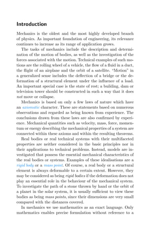
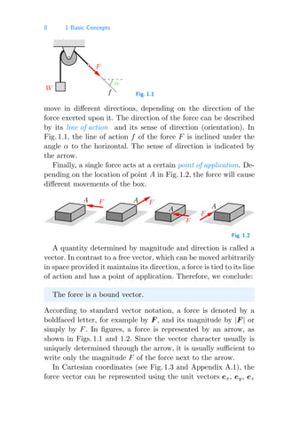
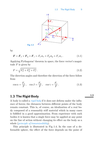
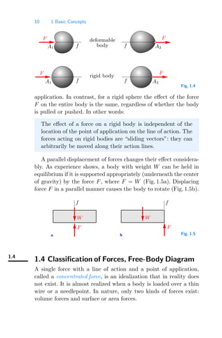
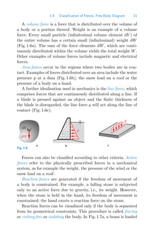
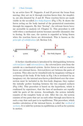
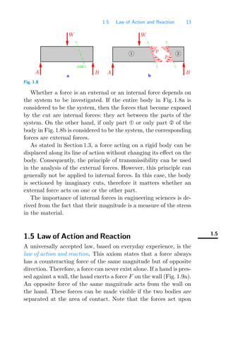
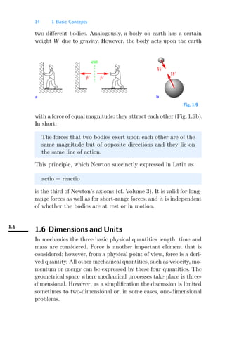
![1.6 Dimensions and Units 15
Associated with length, time, mass and force are their dimen-
sions [l], [t], [M] and [F]. According to the international SI unit
system (Système International d
Unités), they are expressed using
the base units meter (m), second (s) and kilogram (kg) and the
derived unit newton (N). A force of 1 N gives a mass of 1 kg the
acceleration of 1 m/s2
: 1 N = 1 kg m/s2
. Volume forces have the di-
mension force per volume [F/l3
] and are measured, for example,
as a multiple of the unit N/m3
. Similarly, area and line forces
have the dimensions [F/l2
] and [F/l] and the units N/m2
and
N/m, respectively.
The magnitude of a physical quantity is completely expres-
sed by a number and the unit. The notations F = 17 N or l =
3 m represent a force of 17 newtons or a distance of 3 meters,
respectively. In numerical calculations units are treated in the
same way as numbers. For example, using the above quantities,
F · l = 17 N · 3 m = 17 · 3 Nm = 51 Nm. In physical equations,
each side and each additive term must have the same dimension.
This should always be kept in mind when equations are formulated
or checked.
Very large or very small quantities are generally expressed by
attaching prefixes to the units meter, second, newton, and so forth:
k (kilo = 103
), M (mega = 106
), G (giga = 109
) and m (milli
= 10−3
), μ (micro = 10−6
), n (nano = 10−9
), respectively; for
example: 1 kN = 103
N.
Table 1.1
U.S. Customary Unit SI Equivalent
Length 1 ft 0.3048 m
1 in (12 in = 1 ft) 25.4 mm
1 yd (1 yd = 3 ft) 0.9144 m
1 mi 1.609344 km
Force 1 lb 4.4482 N
Mass 1 slug 14.5939 kg](https://image.slidesharecdn.com/engineeringmechanics1statics-250430055049-c59c4287/85/Engineering-Mechanics-1-Statics-chaptetrs-pdf-24-320.jpg)

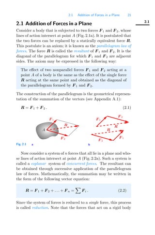
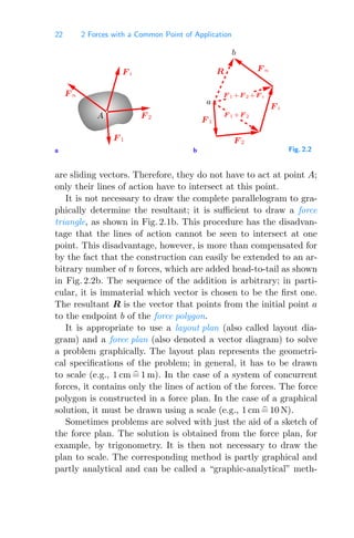
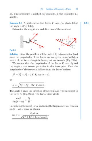
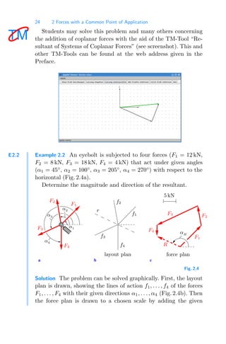
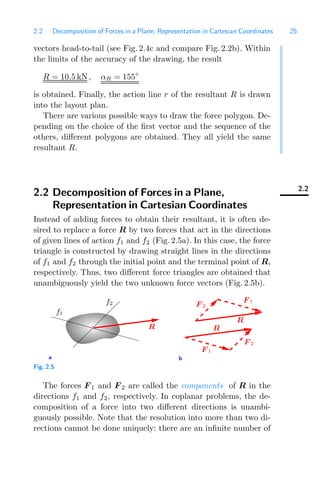
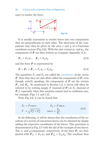
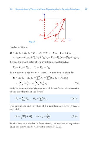
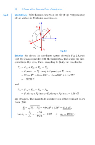
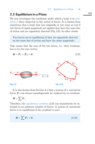
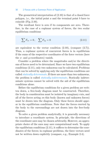
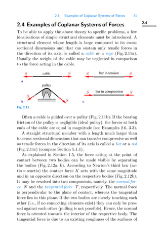
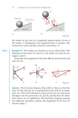
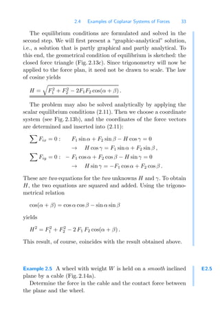
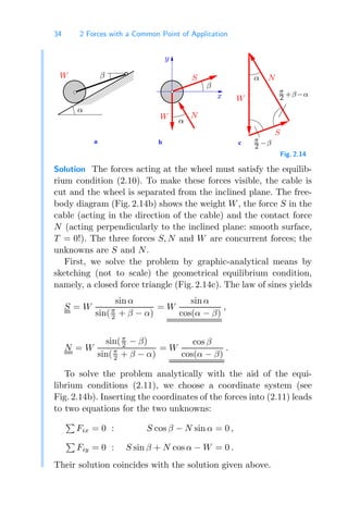
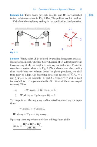
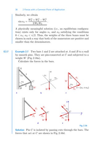
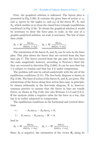
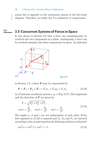
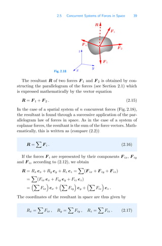
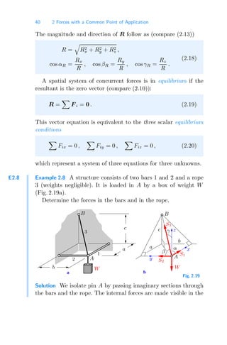
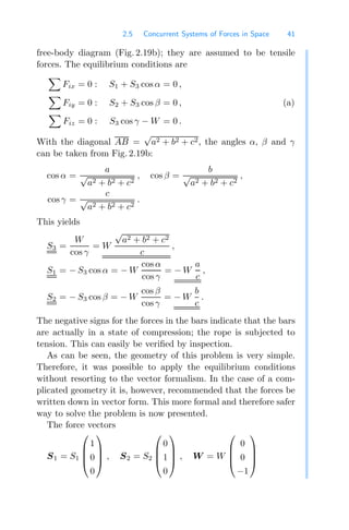
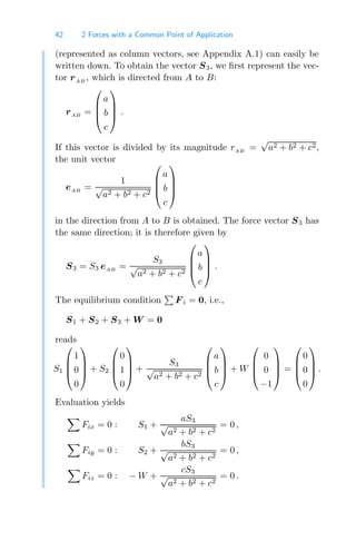
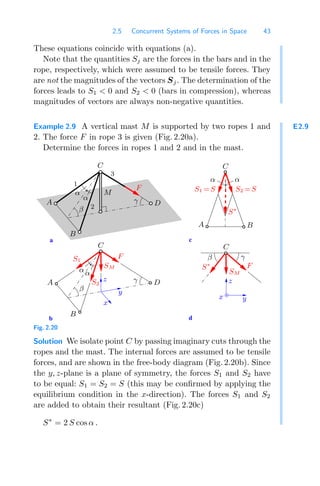
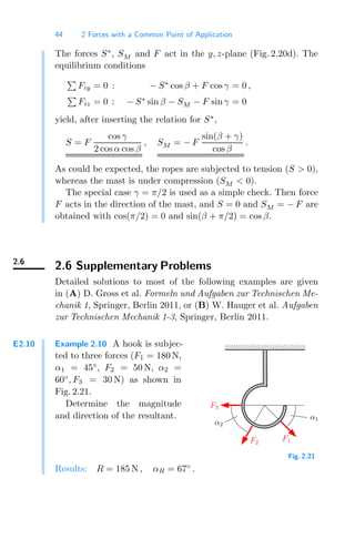
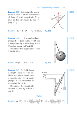
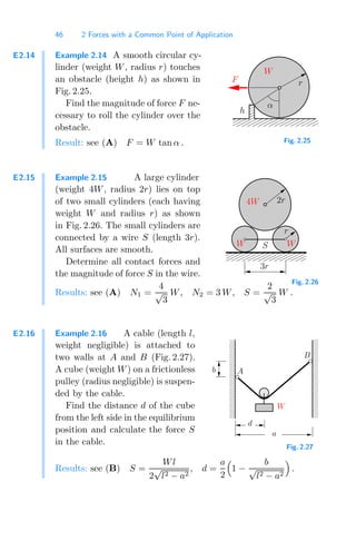
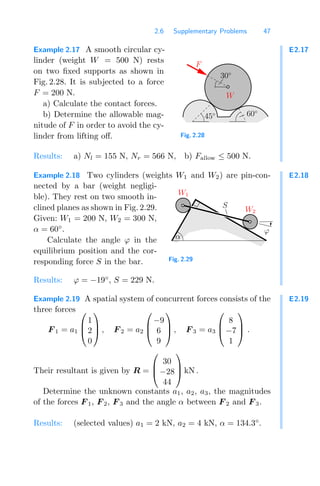
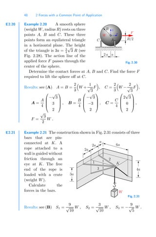
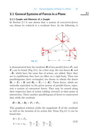
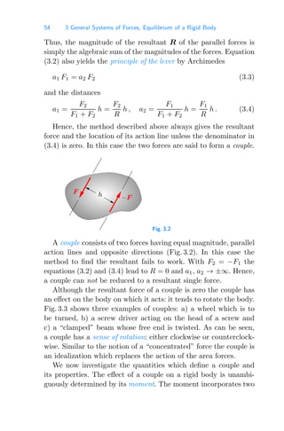
![3.1 General Systems of Forces in a Plane 55
0000
0000
0000
0000
0000
0000
0000
1111
1111
1111
1111
1111
1111
1111
000
000
000
000
000
000
000
000
111
111
111
111
111
111
111
111
c
a b
F
F
F
F
F
F
F
F
F
F
h
h h h
h
Fig. 3.3
quantities: first, its magnitude M which is given by the product
of the perpendicular distance h of the action lines (Fig. 3.2) and
the magnitude F of the forces
M = h F , (3.5)
and, secondly, its sense of rotation. In the figures, the sense of
rotation is represented by a curved arrow ( or ). The quanti-
ties magnitude M and sense of rotation indicate that a couple
moment is a vector in three-dimensional space. The moment has
the dimension length times force [l F], and is expressed, for ex-
ample, in the unit Nm. In order to avoid confusion with the unit
mN
= Milli-Newton, the sequence of the units of length and force
is exchanged: Nm
= Newton-Meter.
Fig. 3.4 shows that a couple with a given moment can be pro-
duced by arbitrarily many different pairs of forces. If the forces K
and −K are added to the given couple (forces F, perpendicular
distance h) a statically equivalent couple is obtained (forces F
,
perpendicular distance h
). The couple moment, i.e., the sense of
rotation and the magnitude of the moment
M = h
F
= (h sin α)
F
sin α
= h F](https://image.slidesharecdn.com/engineeringmechanics1statics-250430055049-c59c4287/85/Engineering-Mechanics-1-Statics-chaptetrs-pdf-63-320.jpg)
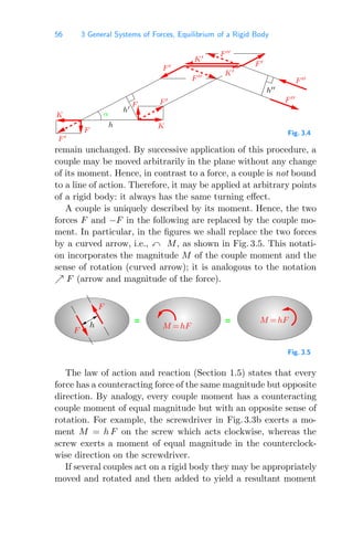
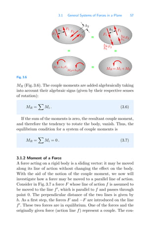
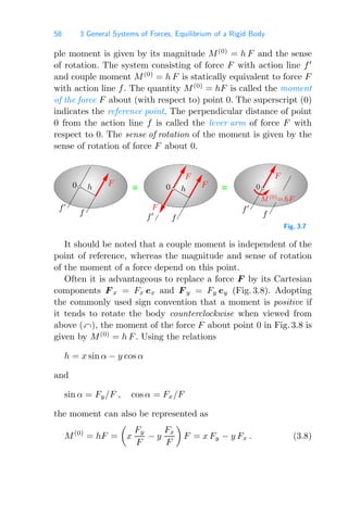
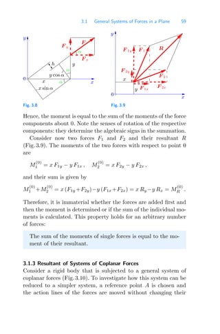
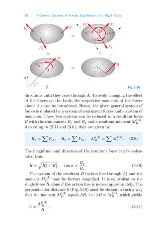
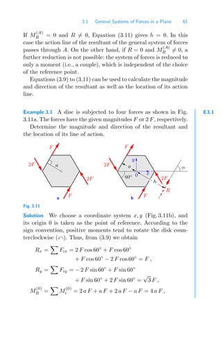
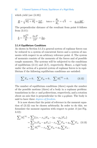
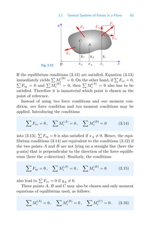
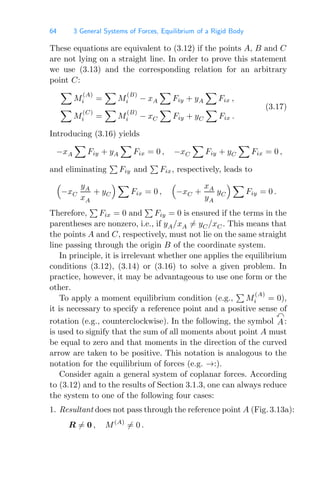
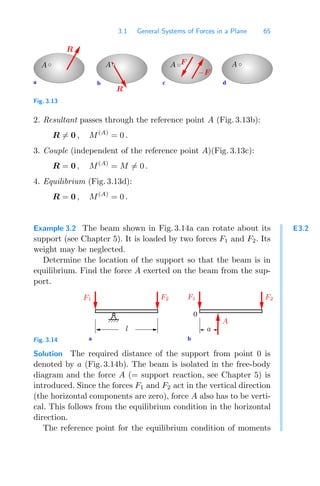
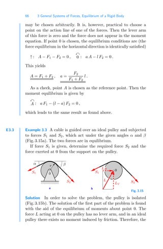
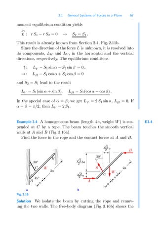
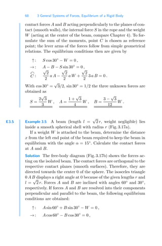
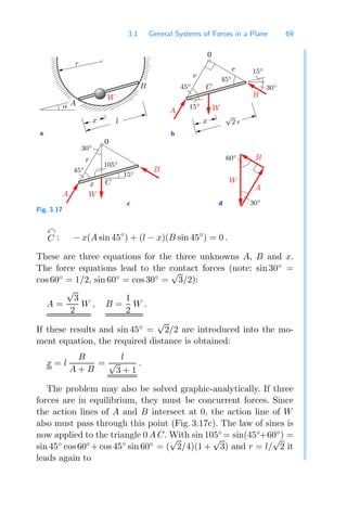
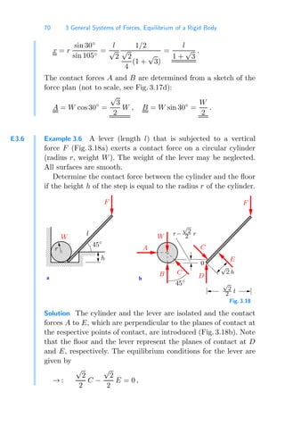
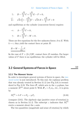
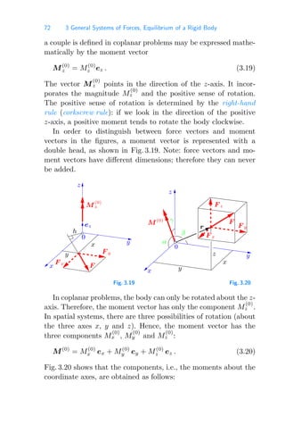
![3.2 General Systems of Forces in Space 73
M(0)
x = yFz −zFy, M(0)
y = zFx −xFz, M(0)
z = xFy −yFx. (3.21)
The magnitude and direction of the moment vector are given by
|M(0)
| = M(0)
=
[M
(0)
x ]2 + [M
(0)
y ]2 + [M
(0)
z ]2 ,
cos α =
M
(0)
x
M(0)
, cos β =
M
(0)
y
M(0)
, cos γ =
M
(0)
z
M(0)
.
(3.22)
Formally, the moment vector M(0)
may be represented by the
vector product
M(0)
= r × F , (3.23)
where vector r is the position vector pointing from the reference
point 0 to the point of application of force F , i.e., to an arbitrary
point on the action line of F . With
r = x ex + y ey + z ez , F = Fx ex + Fy ey + Fz ez
and the following cross-products (compare Appendix A.1),
ex × ex = 0 , ex × ey = ez , ex × ez = −ey ,
ey × ex = −ez , ey × ey = 0 , ey × ez = ex ,
ez × ex = ey , ez × ey = −ex , ez × ez = 0
equation (3.23) yields
M(0)
= (x ex + y ey + z ez) × (Fx ex + Fy ey + Fz ez)
= (y Fz − z Fy) ex + (z Fx − x Fz) ey + (x Fy − y Fx) ez
= M(0)
x ex + M(0)
y ey + M(0)
z ez . (3.24)
According to the properties of a cross-product, the moment vec-
tor M(0)
is perpendicular to the plane determined by r and F
(Fig. 3.21). Its magnitude is numerically equal to the area of the
parallelogram formed by r and F :
M(0)
= r F sin ϕ = h F . (3.25)](https://image.slidesharecdn.com/engineeringmechanics1statics-250430055049-c59c4287/85/Engineering-Mechanics-1-Statics-chaptetrs-pdf-81-320.jpg)
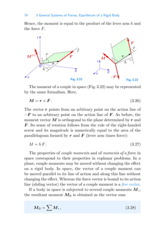
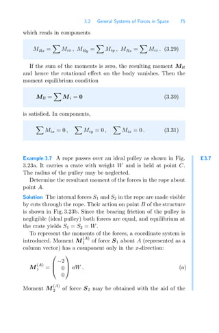
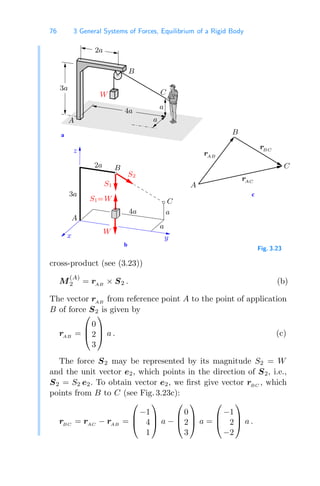
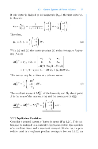
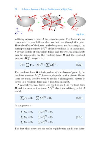
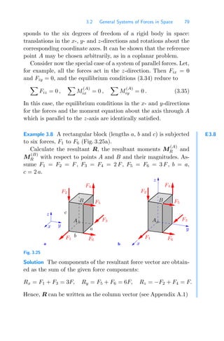
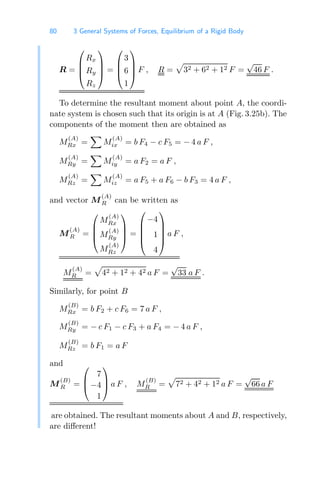
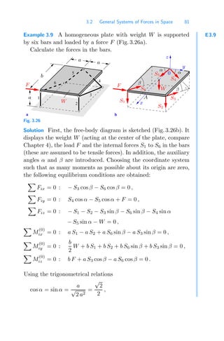
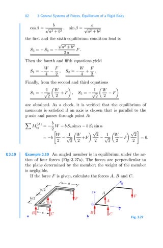
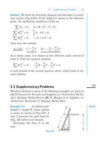
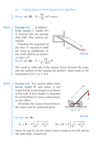
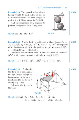
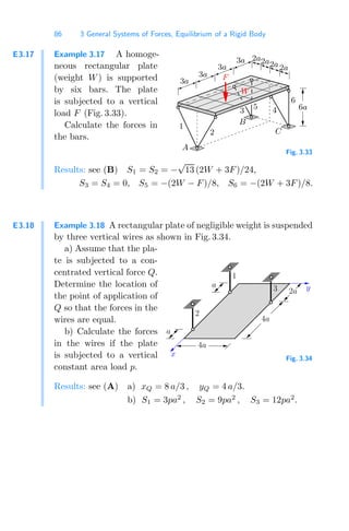
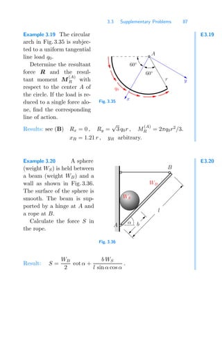
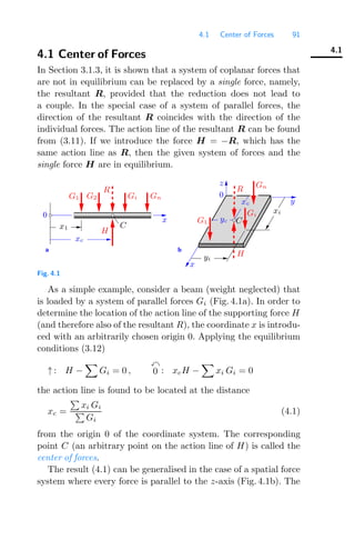
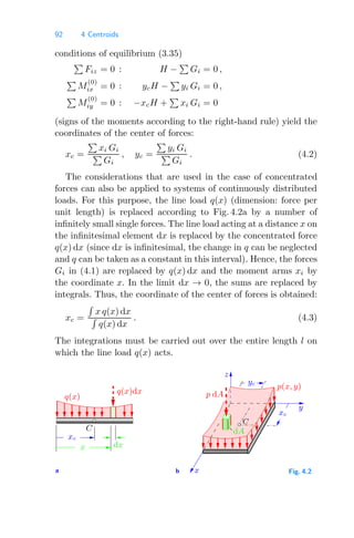
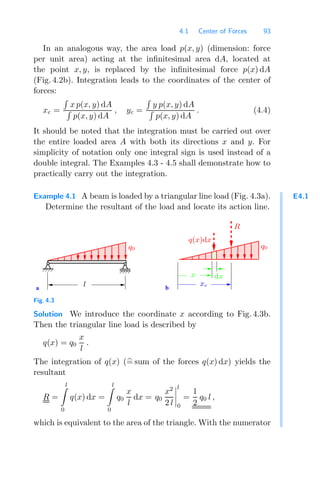
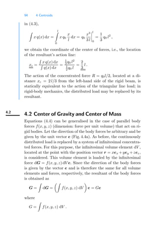
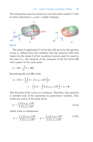
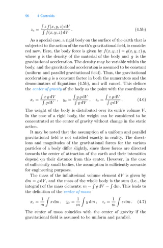
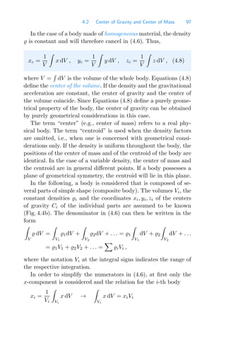
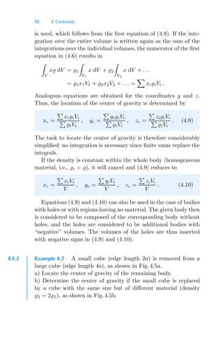
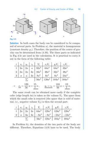
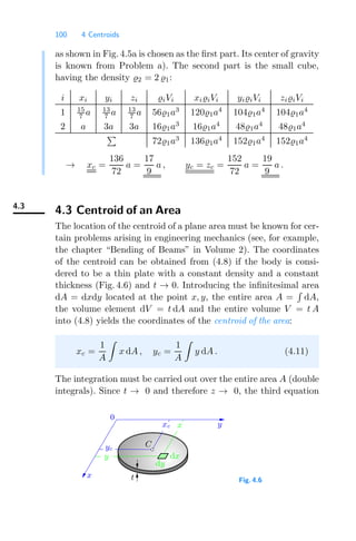
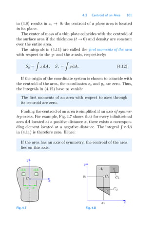
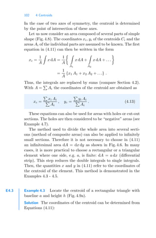
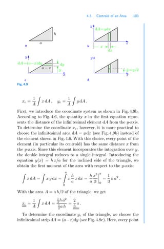
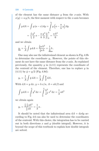
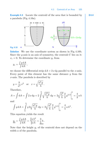
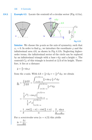
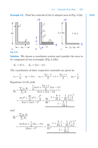
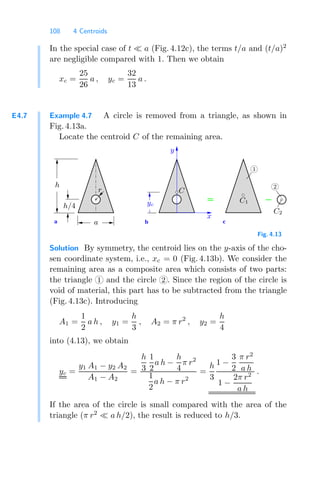
![4.3 Centroid of an Area 109
Table 4.1 Location of Centroids
Area Location of Centroid
Rectangular triangle
x
y
C
a
h A =
1
2
ah xc =
2
3
a, yc =
h
3
Arbitrary triangle
x
y
x3, y3
x1, y1
C
x2, y2
A =
1
2
[(x2 − x1)(y3 − y1)
−(x3 − x1)(y2 − y1)]
xc =
1
3
(x1 + x2 + x3)
yc =
1
3
(y1 + y2 + y3)
Parallelogram
h
C
a
A = a h
C is determined by
the intersection of
the diagonals
Trapezium C is located at
the median line
x
y
h
C
b
a
A =
h
2
(a + b) yc =
h
3
a + 2 b
a + b
Circular sector
y
x
C
r
α
α
A = α r2
xc =
2
3
r
sin α
α
Semicircle
y
x
r
C A =
π
2
r2
xc =
4 r
3 π](https://image.slidesharecdn.com/engineeringmechanics1statics-250430055049-c59c4287/85/Engineering-Mechanics-1-Statics-chaptetrs-pdf-117-320.jpg)
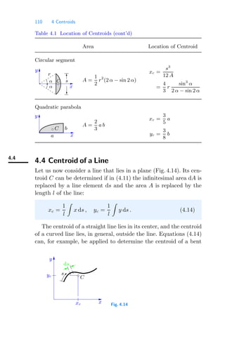
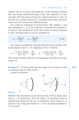
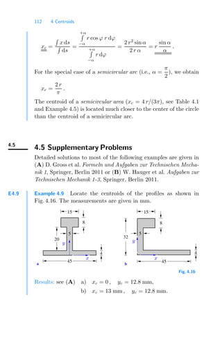
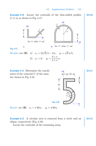
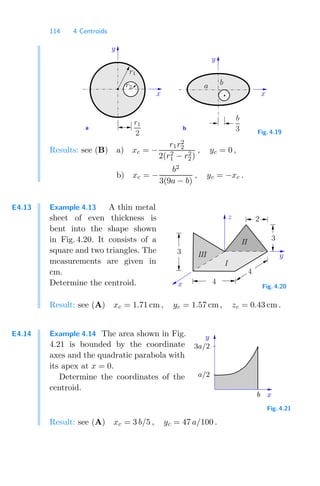
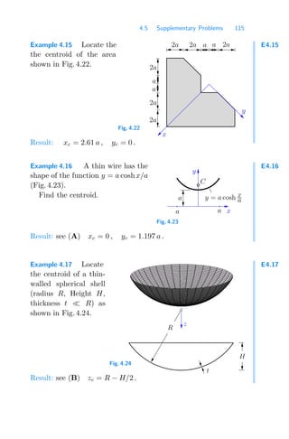
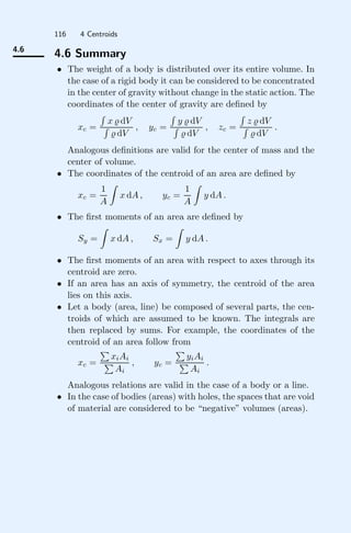

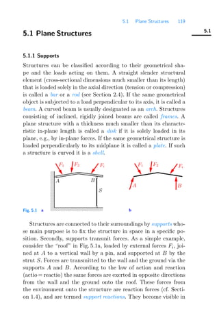
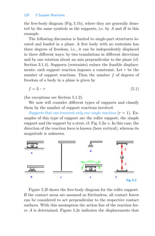
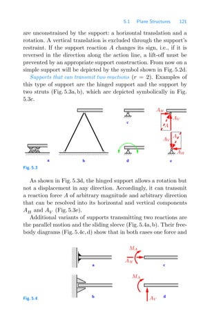
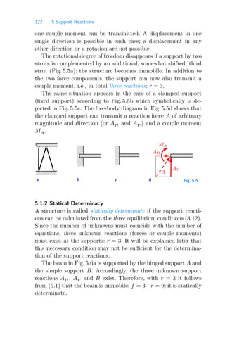
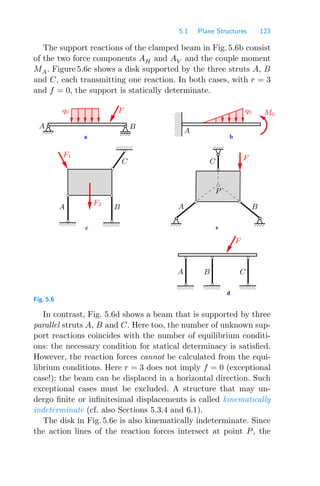
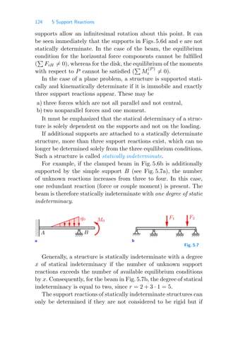
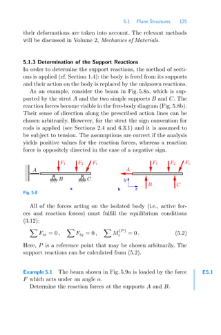
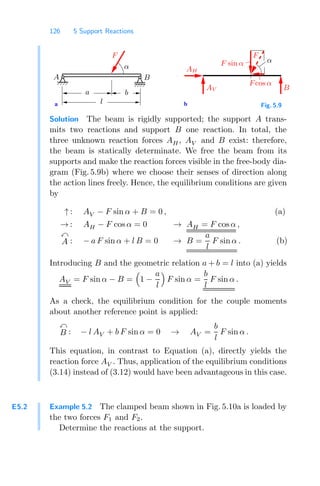
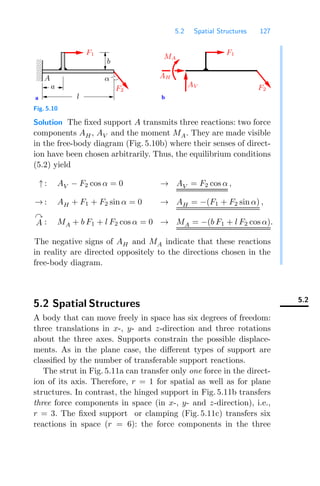
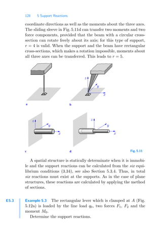
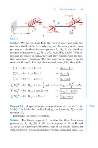
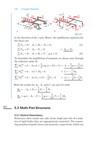
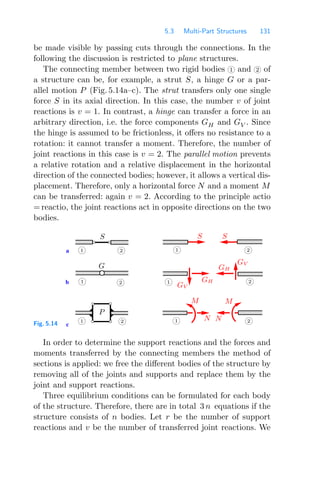
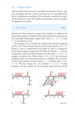
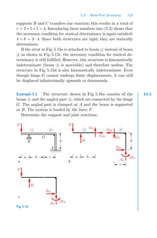
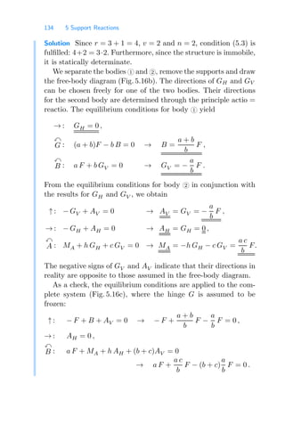
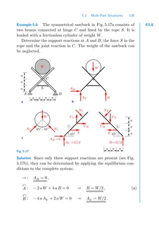
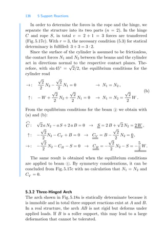
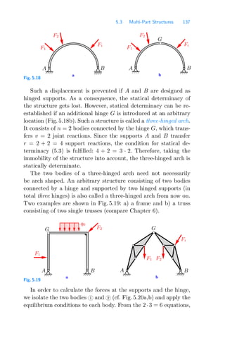
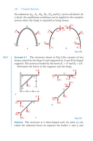
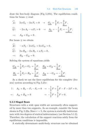
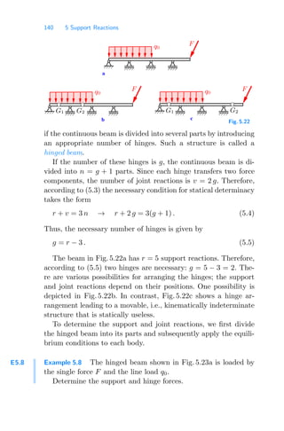
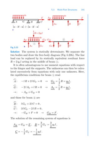
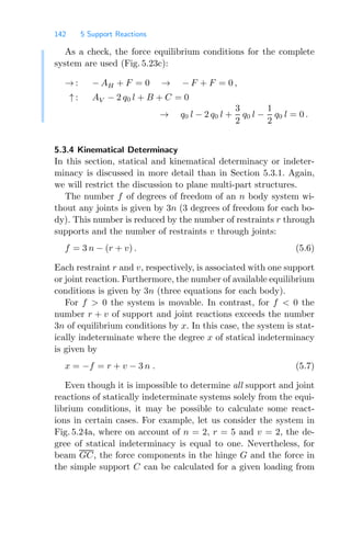
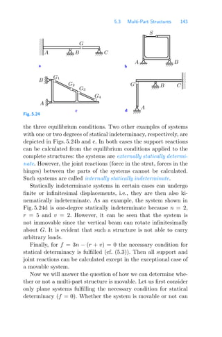
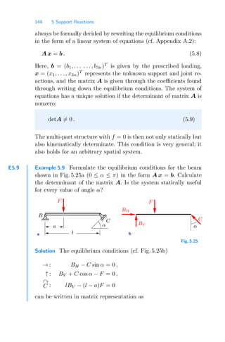
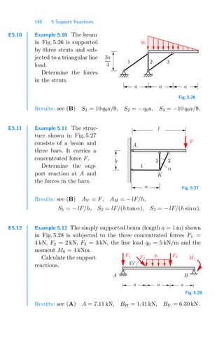
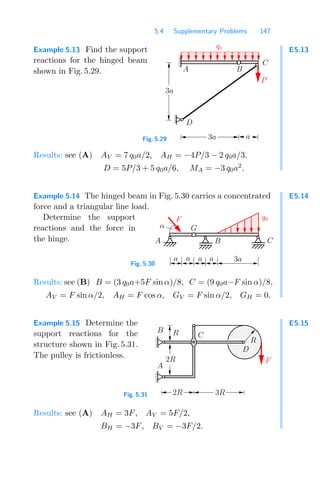
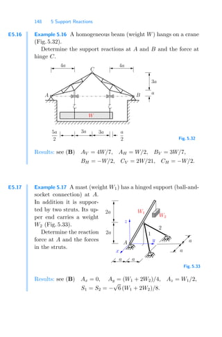
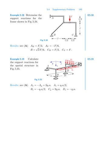

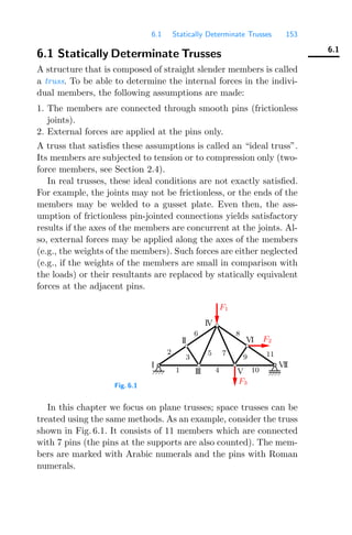
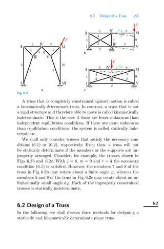
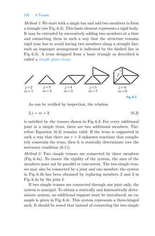
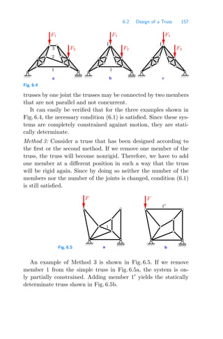
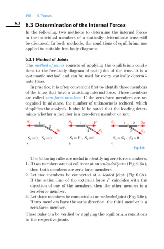
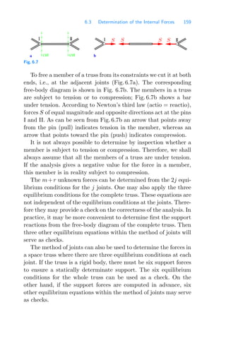
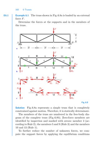
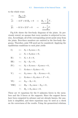
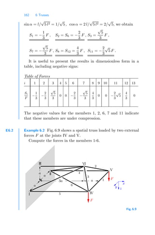
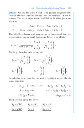
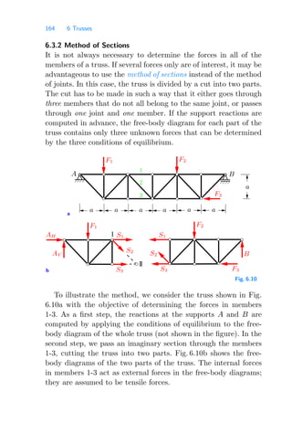
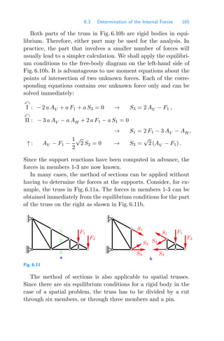
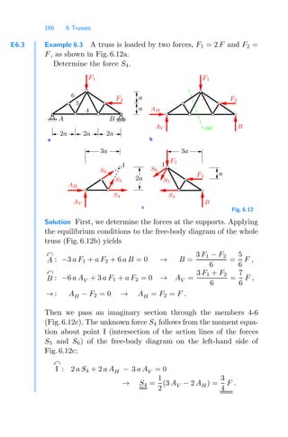
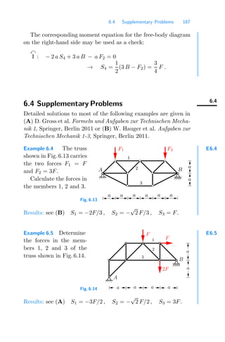
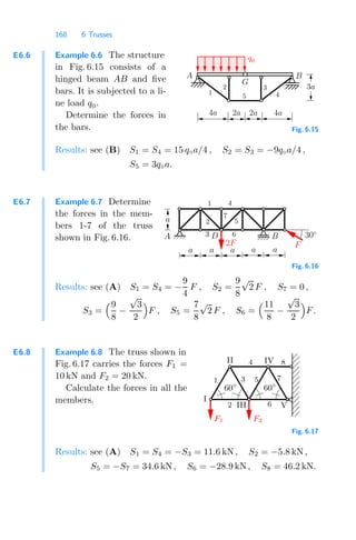
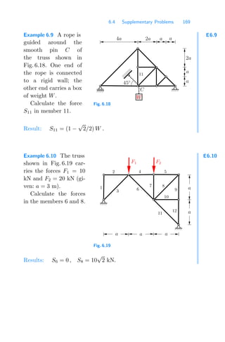
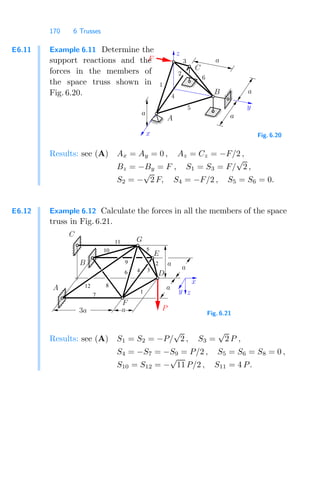

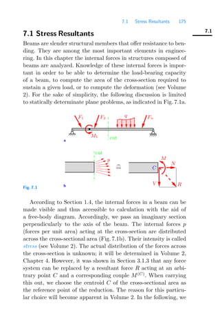
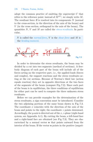
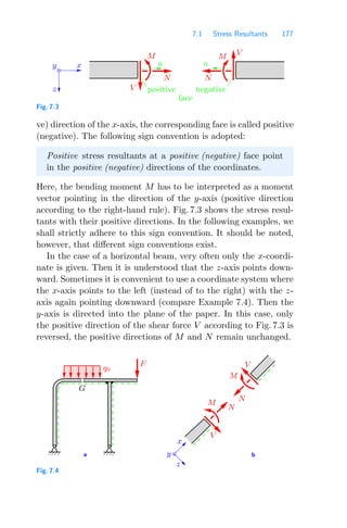
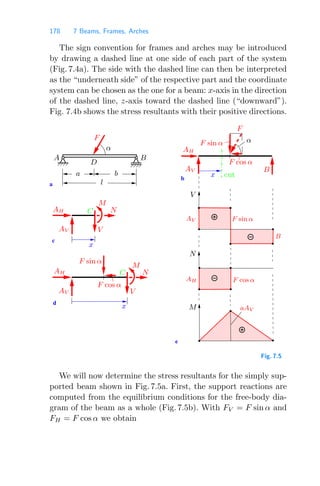
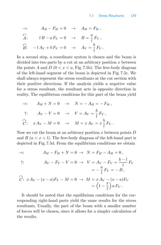
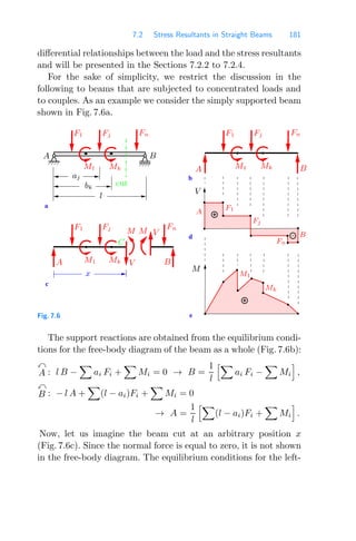
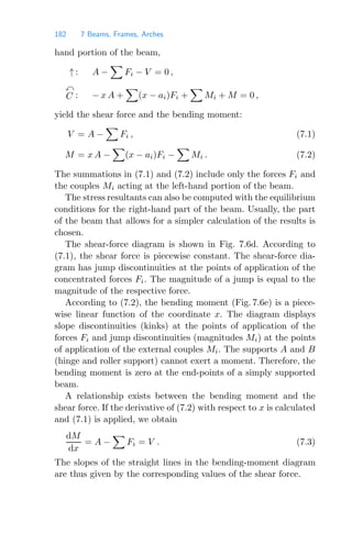
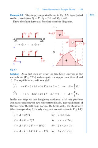
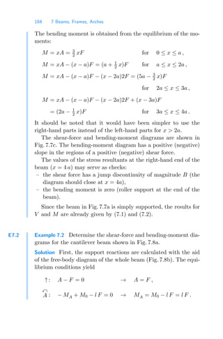
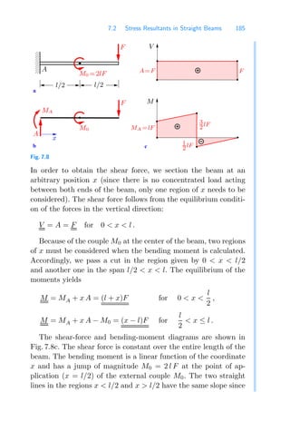
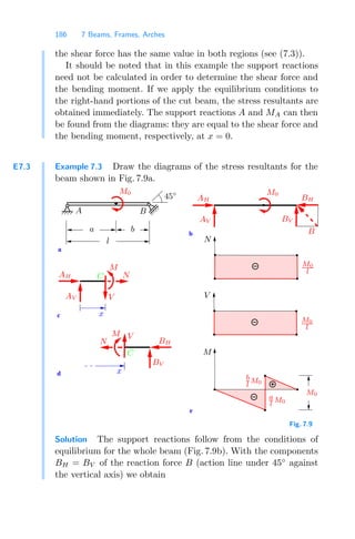
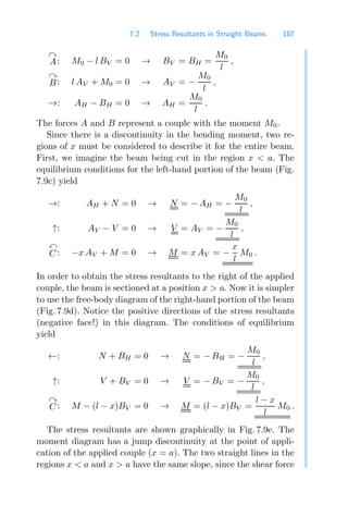
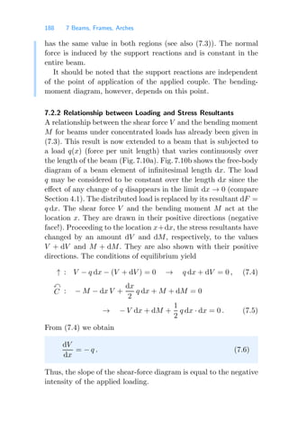
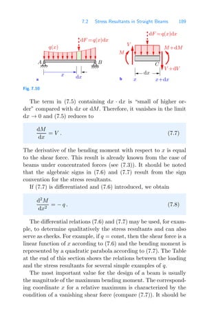
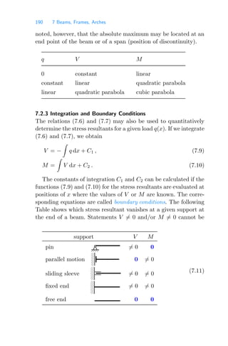
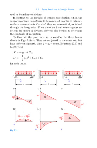
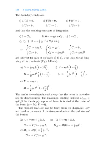
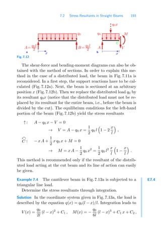
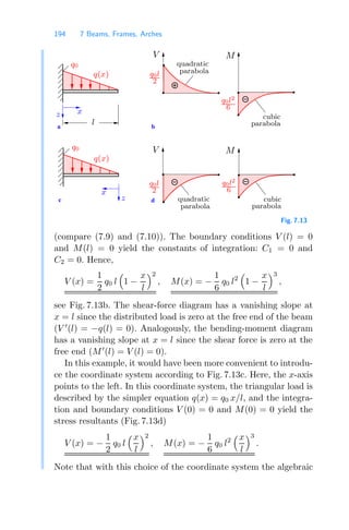
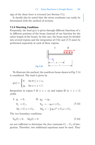
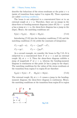
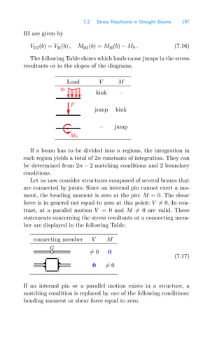
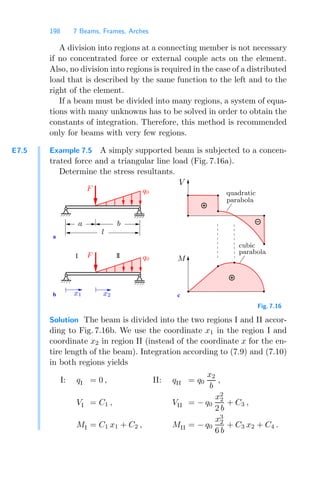
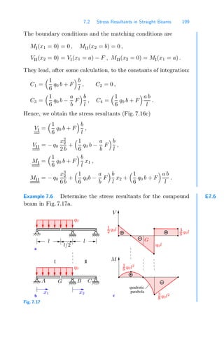
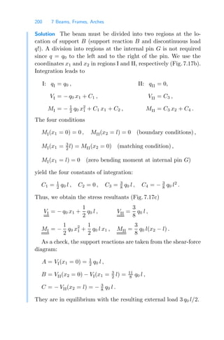
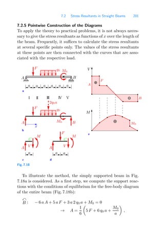
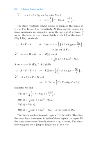
![7.2 Stress Resultants in Straight Beams 203
Accordingly, the bending moment varies linearly in the regions
I, II, IV and V, and it is described by a quadratic parabola in
region III (compare the Table in Section 7.2.2). The diagram shows
a jump in the slope at x = a. Since the shear-force diagram is
continuous at x = 2 a and x = 4 a, the moment diagram has no
jumps in the slopes at these points (V = dM/dx). The external
couple M0 causes a jump in the diagram at x = 5 a.
Fig. 7.18e shows the diagrams of the stress resultants. The max-
imum bending moment is located at the position of the vanishing
shear force.
E7.7
Example 7.7 Draw the diagrams of the stress resultants for the
structure in Fig. 7.19a (a = 0.5 m, q0 = 60 kN/m, F = 80 kN,
M0 = 10 kNm).
c
b
a
0
0
0
0
1
1
1
1
quadratic
parabola
cubic
parabola
quadratic
parabola
MB
B
A
q0
a
x
F
A
2q0a
G
M0
F
MB
B
G
2a
M0
B
A
M0 G
q0a
a
2a
G
F
1 2
50
-50
-100
-25
-50
V
M
[kN]
[kNm]
Fig. 7.19
Solution First, we compute the support reactions and the force in
the internal pin G (the horizontal components are zero). The equi-
librium conditions for the free-body diagrams of the two portions
of the structure (Fig. 7.19b) yield
1
A :
2
3
a q0 a + M0 − a 2 q0 a − 2 a G = 0](https://image.slidesharecdn.com/engineeringmechanics1statics-250430055049-c59c4287/85/Engineering-Mechanics-1-Statics-chaptetrs-pdf-210-320.jpg)
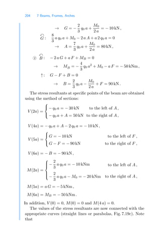
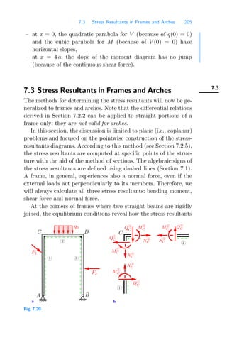
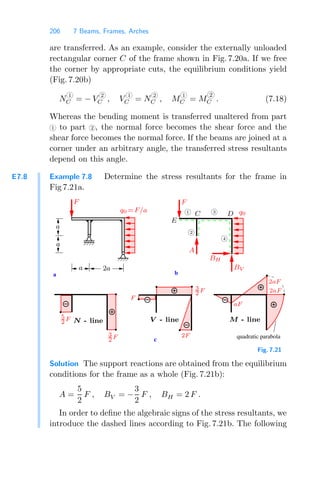
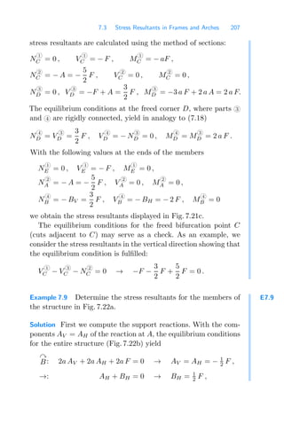
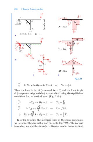
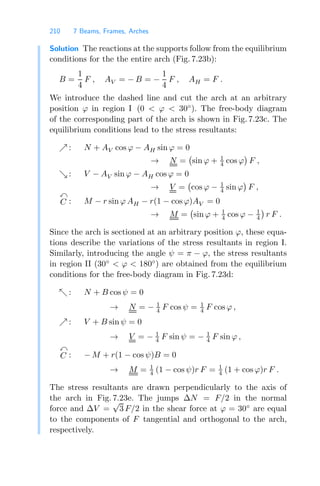
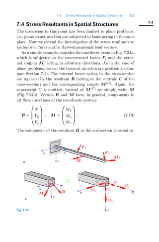
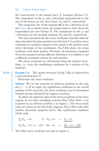
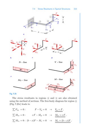
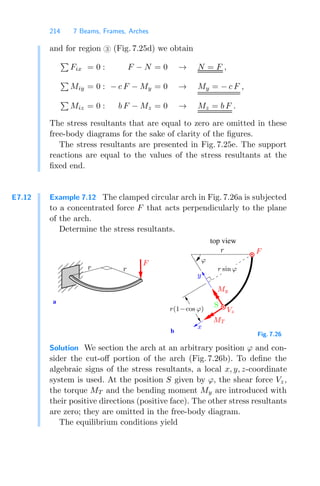
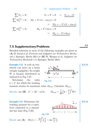
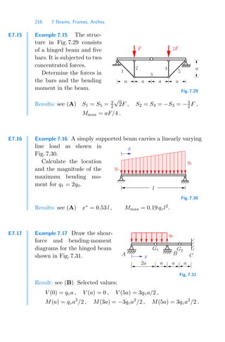
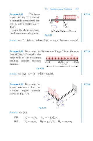
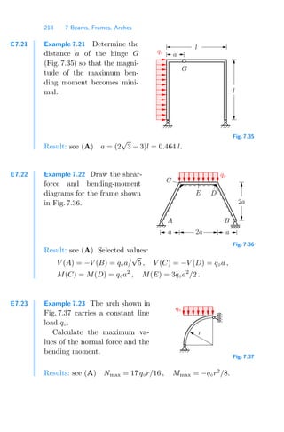
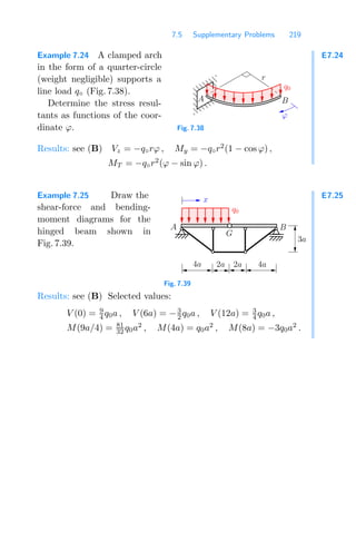
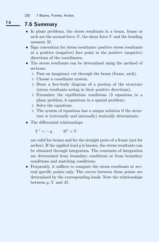

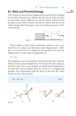
![224 8 Work and Potential Energy
According to (A.19), this product of the vectors F and dr is given
by the scalar value
dU = |F ||dr| cos α = (F cos α)dr = F(dr cos α) . (8.2)
Thus, the work dU is the displacement dr multiplied by the force
component F cos α in the direction of the displacement. Alterna-
tively, it may be interpreted as the product of the force F and
the component of the displacement dr cos α in the direction of the
force (Fig. 8.2b). If force and displacement are orthogonal (α =
π/2), then no work will be done: dU = 0.
The work done along an arbitrary path (Fig. 8.2a) from point
1 to point 2 can be determined from the line-integral
U =
dU =
2
1
F · dr . (8.3)
Work has the dimension [F l] and is given in the unit named after
the physicist James Prescott Joule (1818–1889):
1 J = 1 Nm.
The magnitude and direction of the force F in (8.3) may de-
pend on the position vector r, i.e., F = F (r). Therefore, the
expression “work= force × distance” is only valid when both vec-
tors F and dr permanently have the same direction (α = 0), and
the magnitude of F is constant.
As an example, let us consider a system of two bodies with
weights W and Q, respectively, connected by an unstretchable
cable (Fig. 8.3). If the body on the left side undergoes a downward
displacement of length ds, then the body on the right side will
be pulled the same length upward along the inclined plane. The
work done by weight W is then given by dUW = W ds, since the
directions of the force and the displacement coincide. Only the
component Q sin α in the direction of the displacement is taken
into account for the work done by Q, since the component of a
force perpendicular to the direction of the displacement does no](https://image.slidesharecdn.com/engineeringmechanics1statics-250430055049-c59c4287/85/Engineering-Mechanics-1-Statics-chaptetrs-pdf-231-320.jpg)
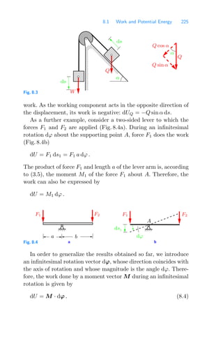
![226 8 Work and Potential Energy
The work done by a moment vector M during a finite rotation of
the body on which it acts, follows from integration:
U =
dU =
M · dϕ . (8.5)
This equation is analogous to the expression (8.3) for the work of
a force. If M and dϕ are parallel, then it follows from (8.4) that
dU = Mdϕ. If, in addition, M is constant during a finite rotation
ϕ, then (8.5) yields U = M ϕ.
Since an angle is dimensionless, moment and work (although
they are different physical quantities) have the same dimension
[F l].
r
x
z
y W
dr
1
2 Fig. 8.5
Now a special case of a constant force is considered, namely, the
weight W of a body (dead load) in the vicinity of the earth’s sur-
face (Fig. 8.5). Let the coordinate z point perpendicularly outward
from the earth’s surface, then the force vector is given by
W = − W ez .
With the change of the position vector
dr = dx ex + dy ey + dz ez
and
ez · ex = ez · ey = 0 , ez · ez = 1 (see (A.22))
we obtain from (8.1)](https://image.slidesharecdn.com/engineeringmechanics1statics-250430055049-c59c4287/85/Engineering-Mechanics-1-Statics-chaptetrs-pdf-233-320.jpg)
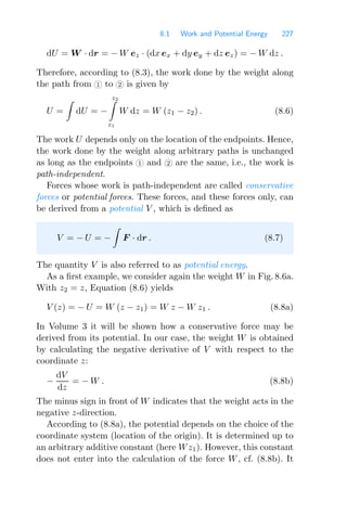
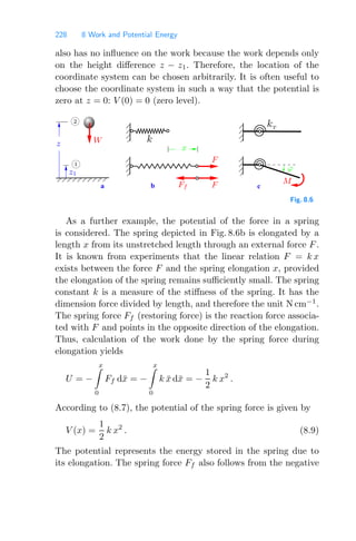
![8.2 Principle of Virtual Work 229
derivative of V with respect to the coordinate x:
Ff = −
dV
dx
= − k x .
Consider now a linear torsion spring as depicted in Fig. 8.6c.
There is a linear relation M = kT
ϕ between the moment M and
the angle of rotation ϕ. This relation is analogous to F = k x
in the foregoing case. The torsion spring constant kT
has the
dimension [Fl] and therefore the unit N cm or a multiple of it. If
in Equation (8.9), k is replaced by kT and x by ϕ, the potential
of the moment of a torsion spring is obtained:
V =
1
2
kT
ϕ2
. (8.10)
8.2
8.2 Principle of Virtual Work
Up to this point in the chapter we have calculated the work done
by a force when the point of application actually moves along a
path. However, the concept of work can also be applied to statics,
where no displacements occur. In this framework, actual displace-
ments must be replaced by virtual displacements. Virtual displa-
cements are displacements (or rotations) that are
a) fictitious, i.e., do not exist in reality,
b) infinitesimally small,
c) geometrically (kinematically) admissible, i.e. consistent with
the constraints of the system.
In order to distinguish virtual displacements from real displa-
cements dr, we denote virtual displacements as δr, i.e., with the
δ-symbol, taken from the calculus of variations. Accordingly, the
virtual work done by forces or moments during a virtual displace-
ment is written as
δU = F · δr (compare (8.1)),
δU = M · δϕ (compare (8.4)).
We now reconsider the two-sided lever (Fig. 8.7a) and calculate
the work done during a virtual displacement. A virtual displace-](https://image.slidesharecdn.com/engineeringmechanics1statics-250430055049-c59c4287/85/Engineering-Mechanics-1-Statics-chaptetrs-pdf-236-320.jpg)