SlideShare a Scribd company logo
1 of 82
%29
%27
SafeAssign Originality Report
Cybersecurity Planning & Mgmt - 201951 - CRN201 - Wag… •
Self-Directed Research
%56Total Score: High risk
Sudheer Raavi
Submission UUID: 11094fc4-a843-3339-deaa-9e926a968bf3
Total Number of Reports
1
Highest Match
56 %
Self Directed Research - Dee…
Average Match
56 %
Submitted on
02/27/20
07:30 PM EST
Average Word Count
436
Highest: Self Directed Resear…
%56Attachment 1
Institutional database (3)
Student paper Student paper Student paper
Internet (3)
upguard wikipedia airsassociation
Top sources (3)
Excluded sources (0)
View Originality Report - Old Design
Word Count: 436
Self Directed Research - Deep and Dark Web.docx
2 6 4
3 1 5
3 upguard 2 Student paper 6 Student paper
Source Matches (16)
wikipedia 100%
Student paper 65%
wikipedia 100%
Student paper 65%
wikipedia 100%
wikipedia 100%
Student paper 66%
Student paper 71%
Running head: DEEP WEB VS. DARK WEB 1
DEEP WEB VS. DARK WEB 2
Deep Web vs. Dark Web
Name: Sudheer Raavi
Institution: New England College
Course: Cybersecurity Planning & Mgmt
Deep Web vs. Dark Web
The deep web and dark web are used interchangeably but have
different meanings. The deep web refers to the pages that are
not indexed, implying that
any search engine will fail to return them after searching.
Search engine crawlers cannot see these pages as they are
invisible. Deep web, therefore, works in
one major way, which is obscurity. Obscurity means the
inability to locate an internet resource using any major search
engine. The deep web is achieved
by adding a preferable robots.txt file to the website (Sen, 2019).
It prevents crawlers from indexing such a site and eventually
prevents the pages from dis-
playing the search engine results pages (SERPS). On the other
hand, the dark web refers to the various encrypted overlay and
self-contained networks that
live on top of the internet and inaccessible unless one has the
right protocol and tools. By comparison, the deep web is larger
than the dark web.
Dark web sites are only in thousands. Usually, the sites in the
Dark Web are differentiated by the use of encryption software,
which makes any user and the lo-
cation secret. It is the reason for illegal activities that are
dominant on the dark web because users can hide their identities
(Sussman, 2018). The owners of the
illegal websites also conceal their location and data transfer
occurs anonymously. Overall, the dark web houses various
illegal activities like firearms, drug
deals, gambling, and other illicit trades. Therefore, the deep
web includes various parts of legitimate websites like schools,
banks, and other institutional web-
sites that require logins. Also, it can be mainstream web like
Netflix pages since they are personalized for the users and the
URLs are not indexed (Sen, 2019).
The dark web, however, is a smaller portion since the sites are
intentionally hidden and unreachable through standard search
engines. A famous element that
offers access to the dark web is the TOR network. TOR network
is anonymous and can only access through a specific web
browser, known as the TOR browser.
Therefore, the dark web has illegal activities due to the
anonymity of the TOR network.
References
Sen, K. (2019). Deep Web vs Dark Web: What's the difference?.
Upguard. Retrieved from https://www.upguard.com/blog/dark-
web-vs-deep-web
Sussman, B. (2018). Dark Web vs. Deep Web: What Is the
Difference? Securewrold. Retrived from
https://www.secureworldexpo.com/industry-
news/dark-web-vs-deep-web
1 2
1 2
1
1
2
2
2
3
4 5
3 6
3 6
1
Student paper
DEEP WEB VS.
Original source
"The Deep Web vs
2
Student paper
DARK WEB 1
Original source
DEEP WEB 1
1
Student paper
DEEP WEB VS.
Original source
"The Deep Web vs
2
Student paper
DARK WEB 2
Original source
DEEP WEB 2
1
Student paper
Deep Web vs.
Original source
"The Deep Web vs
1
Student paper
Deep Web vs.
Original source
"The Deep Web vs
2
Student paper
The deep web and dark web are used
interchangeably but have different
meanings.
Original source
The terms Dark Web and Deep Web
can be used interchangeably, but they
differ
2
Student paper
Obscurity means the inability to locate
an internet resource using any major
search engine.
Original source
Obscurity is the inability to locate an in-
ternet resource in the search engines
Student paper 66%
upguard 69%
Student paper 67%
airsassociation 86%
upguard 100%
Student paper 100%
upguard 100%
Student paper 70%
2
Student paper
It prevents crawlers from indexing such
a site and eventually prevents the
pages from displaying the search en-
gine results pages (SERPS).
Original source
Fie to a website, which prevents the
search engine crawlers from indexing
the site, hence preventing pages dis-
playing in the results
3
Student paper
On the other hand, the dark web refers
to the various encrypted overlay and
self-contained networks that live on top
of the internet and inaccessible unless
one has the right protocol and tools.
Original source
The dark web refers to any number of
self-contained, encrypted overlay net-
works that live on top of the internet,
inaccessible save for special tools and
protocols, hence dark
4
Student paper
By comparison, the deep web is larger
than the dark web.
Original source
That is Deep Web and Dark Web
5
Student paper
Dark web sites are only in thousands.
Original source
Dark Web sites number only in the
thousands
3
Student paper
Deep Web vs Dark Web: What's the
difference?.
Original source
Deep Web vs Dark Web What's the
difference
6
Student paper
Retrieved from https://www.upguard.-
com/blog/dark-web-vs-deep-web
Original source
Retrieved from https://www.upguard.-
com/blog/dark-web-vs-deep-web
3
Student paper
Dark Web vs.
Original source
Dark Web vs
6
Student paper
Retrived from https://www.secure-
worldexpo.com/industry-news/dark-
web-vs-deep-web
Original source
Retrieved from https://www.upguard.-
com/blog/dark-web-vs-deep-web
4 Return and Risk
Learning Goals
After studying this chapter, you should be able to:
1. LG 1 Review the concept of return, its components, the
forces that affect the level of return, and historical returns.
2. LG 2 Discuss the role of the time value of money in
measuring return and defining a satisfactory investment.
3. LG 3 Describe real, risk-free, and required returns and the
calculation and application of holding period return.
4. LG 4 Explain the concept and the calculation of an internal
rate of return and how to find growth rates.
5. LG 5 Discuss the key sources of risk that might affect
potential investments.
6. LG 6 Understand the risk of a single asset, risk assessment,
and the steps that combine return and risk.
An old saying often attributed to Mark Twain advises, “Buy
land—they’re not making it anymore.” That bit of folk wisdom
gained enormous popularity during the U.S. real estate boom.
According to the S&P/Case-Shiller Index, which tracks home
prices in 20 large cities, U.S. homeowners saw their property
values increase more than 100% from 2000 to 2005. Over the
same six years, the U.S. stock market (as measured by the S&P
500 Index) lost more than 10% of its value.
Moreover, the tantalizing returns on real estate seemed to come
without much risk. The average home price rose every single
month from July 1996 to May 2006. No wonder, then, that
investing in real estate became fashionable, as evidenced by the
introduction of television shows such as A&E’s Flip This
House. It seemed that no one could lose money by investing in
residential real estate.
Unfortunately, home prices began to decline in late summer
2006, and their fall continued through March 2012. Over that
period, average home prices dropped 34% and millions of
properties were lost to foreclosure, reminding homeowners that
investing in real estate has both rewards and risks. After hitting
bottom in March 2012 the S&P/Case-Shiller Index rose 29% by
the end of 2014; however, this rebound lagged behind the S&P
500 Index return of 46% over the same period.
The boom and bust cycles in both the housing and stock markets
over the last decade provide great examples of the almost
inextricable link between risk and return. Some investments
may deliver high returns for several consecutive years, just as
housing did in the mid 2000s, but high returns tend to be
associated with high risks, as investors in housing learned after
2006. This chapter and the next discuss tools that will help you
quantify the tradeoff between risk and return.
(Source: S&P/Case-Shiller price indexes downloaded
from http://www
.standardandpoors.com and http://www.realtytrac.com/, “Year-
End 2014 U.S. Foreclosure Market Report.”)
The Concept of Return
1. LG 1
2. LG 2
People are motivated to invest in a given asset by its expected
return. The return is the level of profit from an investment—that
is, the reward for investing. Suppose you have $1,000 in an
insured savings account paying 2% annual interest, and a
business associate asks you to lend her that much money. If you
lend her the money for one year, at the end of which she pays
you back, your return will depend on the amount of interest you
charge. If you make an interest-free loan, your return will be 0.
If you charge 2% interest, your return will be $20 (0.02 ×
$1,000). Because you are already earning a safe 2% on the
$1,000, it seems clear that to equal that return you should
charge your associate a minimum of 2% interest.
Some investments guarantee a return, but most do not. The
return on a bank deposit insured by the federal government is
virtually certain. The return earned on a loan to your business
associate might be less certain. The size and the certainty of the
expected return are important factors in choosing a suitable
investment.
Components of Return
The return on an investment comes from two sources. One
source is periodic payments, such as dividends and interest. The
other source is the change in the investment’s price. We call
these two components of an investment’s return current
income and capital gains (or capital losses), respectively.
Income
Income may take the form of dividends from stocks or mutual
funds or interest received on bonds. For our purposes, an
investment’s income is the cash that investors periodically
receive as a result of owning the investment.
Investor Facts
Burrito Bonds are Easy to Swallow In the summer of 2014, the
London-based restaurant chain, Chilango, sold bonds to
investors that promised cash interest payments of 8% per year,
plus vouchers for free burritos. Though those burritos
undoubtedly have some value to Chilango’s investors, when we
calculate an investment’s return, we’ll focus on the cash
payments that the investment makes, ignoring any in-kind
payments like free burritos.
(Source: “Will Chilango’s £2m Success Herald an Affordable
Mini Bond
Revolution?” http://www.forbes.com/sites/trevorclawson/2014/0
8/28/will-chilangos-2m-success-herald-an-affordable-mini-
bond-revolution/, accessed April 23, 2015.)
Using the data in Table 4.1, we can calculate the income from
investments A and B, both purchased for $1,000, over a one-
year period of ownership. Investment A provides income of $80,
and investment B pays $120. Solely on the basis of the income
received over the one year, investment B seems preferable.
Capital Gains (or Losses)
The second dimension of return focuses on the change in an
investment’s market value. As noted in Chapter 1, the amount
by which the proceeds from the sale of an investment exceed its
original purchase price is a capital gain. If an investment sells
for less than its original purchase price, a capital loss results.
Table 4.1 Profiles of Two Investments
Investment
A
B
Purchase price (beginning of year)
$1,000
$1,000
Cash received
1st quarter
$ 10
$ 0
2nd quarter
$ 20
$ 0
3rd quarter
$ 20
$ 0
4th quarter
$ 30
$ 120
Total income (for year)
$ 80
$ 120
Sale price (end of year)
$1,100
$ 960
Table 4.2 Total Returns of Two Investments
Investment
Return
A
B
Income
$ 80
$120
Capital gain (loss)
$100
$(40)
Total return
$180
$ 80
We can calculate the capital gain or loss of the investments
shown in Table 4.1. Investment A experiences a capital gain of
$100 ($1,100 sale price −$1,000 purchase price) over the one-
year period. Investment B, on the other hand, earned a $40
capital loss ($960 sale price − $1,000 purchase price).
Combining the capital gain (or loss) with the income (calculated
in the preceding section) gives the total return. Table 4.2 shows
the total return for investments A and B over the year.
Investment A earns a $180 total return, compared to just $80
earned by investment B.
It is generally preferable to use percentage returns rather than
dollar returns. Percentages allow direct comparison of different
sizes and types of investments. Investment A earned an 18%
return ($180 , $1,000); B produced only an 8% return ($80 ,
$1,000). At this point investment A appears preferable, but as
we’ll see, differences in risk might cause some investors to
prefer B.
Watch Your Behavior
Investment Club’s Returns Less Than Advertised In the mid
1990s, an investment club known as the Beardstown Ladies
gained notoriety, at first because they claimed to have earned
higher returns than the overall stock market for more than a
decade. The ladies wrote a best-selling book full of investment
advice, but no where in that book did they discuss how to
calculate an investment’s return. An audit later revealed that the
Beardstown ladies grossly overstated their returns by including
new capital investments as part of their return. After this error
was corrected, the investment’s club trailed the broader stock
market by several percentage points. Knowing how to calculate
returns properly is the first step in assessing an investment’s
performance.
Source: “Where Are They Now: The Beardstown
Ladies,” http://www.wsj .com/articles/SB114596682916135186,
accessed June 29, 2016.
Why Return Is Important
An asset’s return is a key variable in the investment decision
because it indicates how rapidly an investor can build wealth.
Naturally, because most people prefer to have more wealth
rather than less, they prefer investments that offer high returns
rather than low returns if all else is equal. However, we’ve
already said that the returns on most investments are uncertain,
so how do investors distinguish assets that offer high returns
from those likely to produce low returns? One way to make this
kind of assessment is to examine the returns that different types
of investments have produced in the past.
Historical Performance
Most people recognize that future performance is not guaranteed
by past performance, but past data often provide a meaningful
basis for future expectations. A common practice in the
investment world is to look closely at the historical record when
formulating expectations about the future.
Consider the data for ExxonMobil Corporation presented
in Table 4.3. ExxonMobil paid dividends every year from 2005
through 2014. ExxonMobil’s stock price generally rose during
this decade, starting at $51.26 and ending at $92.45. Despite the
overall upward trend, the company’s stock price fell in 2008
and 2009 (largely due to the Great Recession and the
corresponding drop in oil prices), and it declined again in 2014
(largely due to a rapid increase in the supply of oil and
shrinking worldwide demand for oil).
Two aspects of these data are important. First, we can determine
the annual total return generated by this investment over the
past 10 years. The average annual total return earned by
ExxonMobil’s shareholders (column 6) over this period was
9.6%, performance that put ExxonMobil ahead of
Table 4.3 Historical Investment Data for Exxonmobil Corp.
(XOM)
(Source: Dividends and end-of-year closing prices were
obtained from Yahoo! Finance.)
Market Value (Price)
Yearly Total Return
Year
(1) Dividend Income
(2) Beginning of Year
(3) End of Year
(4) (3) − (2) Capital Gain
(5) (1) + (4)
(6) (5) / (2)
2005
$1.14
$ 51.26
$ 56.17
$ 4.91
$ 6.05
11.8%
2006
$1.28
$ 56.17
$ 76.63
$20.46
$ 21.74
38.7%
2007
$1.37
$ 76.63
$ 93.69
$ 17.06
$18.43
24.1%
2008
$1.55
$ 93.69
$ 79.83
−$13.86
−$ 12.31
−13.1%
2009
$1.66
$ 79.83
$ 68.19
−$ 11.64
−$ 9.98
−12.5%
2010
$1.74
$ 68.19
$ 73.12
$ 4.93
$ 6.67
9.8%
2011
$1.85
$ 73.12
$ 84.76
$ 11.64
$ 13.49
18.4%
2012
$2.18
$ 84.76
$ 86.55
$ 1.79
$ 3.97
4.7%
2013
$2.46
$ 86.55
$101.20
$14.65
$ 17.11
19.8%
2014
$2.70
$101.20
$ 92.45
−$ 8.75
−$ 6.05
−6.0%
Average
$1.79
$ 4.12
$ 5.91
9.6%
many other stocks for the same period. Second, observe that
there was considerable variation in ExxonMobil’s return from
one year to the next. The firm’s best year was 2006, during
which its investors earned a total return of 38.7%. But in 2008,
ExxonMobil’s worst year, shareholders lost 13.1%.
[email protected]
Expected Return
In the final analysis, of course, it’s the future that matters when
we make investment decisions. Therefore an
investment’s expected return is a vital measure of its
performance. It’s what you think the investment will earn in the
future that determines what you should be willing to pay for it.
To demonstrate, let’s return to the data in Table 4.3. A naive
investor might estimate ExxonMobil’s expected return to be the
same as its average return from the prior decade, 9.6%. That’s
not necessarily a bad starting point, but it would be wise to ask,
“What contributed to ExxonMobil’s past returns, and is it likely
that the same factors will occur in the future?” Central to
ExxonMobil’s success in the recent past was a generally upward
trend in oil prices. In early 2005, crude oil traded for around
$58 per barrel, but prices rose steadily until they peaked around
$140 per barrel in June 2008. Even though prices fell sharply
for a brief period during the recession, the price of oil did not
fall below $70 at any point from June 2009 to October 2014, so
this was a very favorable period for ExxonMobil. This suggests
that the historical returns shown in Table 4.3 might represent a
better-than-average period for the company. An investor who
believed that oil prices would not continue to move up
indefinitely, but rather would stabilize, might estimate
ExxonMobil’s expected return by looking at its historical
performance during a period of relatively stable oil prices.
Level of Return
The level of return achieved or expected from an investment
will depend on a variety of factors. The key factors are internal
characteristics and external forces.
Famous Failures in Finance Fears of Deflation Worry Investors
For most of your lifetime, prices of most goods and services
have been rising. There are important exceptions, such as the
prices of consumer electronics and computers, but from one
year to the next, the overall price level rose continuously in the
United States from 1955 through 2007. However, as the
recession deepened in 2008, consumer prices in the United
States began to decline, falling in each of the last five months
that year. Countries in the European Union experienced a brief
deflationary period around the same time. The news raised fears
among some investors that the recession might turn into a
depression like the one that had brought about a price decline of
-27% from November 1929 to March 1933. Although prices
began to rise again, fears of deflation resurfaced again in late
2014 and early 2015. Prices in the United States were flat or
down in the first three months of 2015, while countries in the
European Union experienced falling prices for four consecutive
months starting in December 2015.
Critical Thinking Question
1. Suppose you own an investment that pays a fixed return in
dollars year after year. How do you think inflation (rising
prices) or deflation (falling prices) would influence the value of
this type of investment?
Internal Characteristics
Certain characteristics of an investment affect its return. For
investments issued by companies, the important characteristics
include things such as the type of investment (e.g., stocks or
bonds), the quality of the firm’s management, and whether the
firm finances its operations with debt or equity. For example,
investors might expect a different return on the common stock
of a large, well-managed, completely equity-financed plastics
manufacturer than they would anticipate from the common stock
of a small, poorly managed, largely debt-financed clothing
manufacturer. As we will see in later chapters, assessing
internal factors and their impact on return is one important step
in analyzing possible investments.
External Forces
External forces such as Federal Reserve actions, recessions,
wars, and political events may also affect an investment’s
return. None of these are under the control of the issuer of the
investment, and investments react differently to these forces.
For example, if investors expect oil prices to rise, they may
raise their expected return for ExxonMobil stock and lower it
for the stock of an automobile manufacturer that produces gas
guzzlers. Likewise, the economies of various countries respond
to external forces in different ways.
What Is Inflation?
Another external force is the general level of price changes,
either up—inflation—or down—deflation. How inflation (or
deflation) affects investment returns is complex, but it depends
in part on whether investors correctly anticipate the rate of
inflation. Generally speaking, when investors expect inflation to
occur, they will demand higher returns. For example, when we
look back through history, we see that interest rates on bonds
were usually higher in periods when inflation was higher.
However, when investors are caught off guard and the rate of
inflation is higher or lower than they expected, returns on
investments may rise or fall in response. The way that
investment returns respond to unexpected changes in inflation
will vary from one type of investment to another, and that
response can be influenced by investors’ beliefs about how
policymakers will react to changing inflation. For example, if
inflation unexpectedly rises, investors might anticipate that the
Federal Reserve will take action to slow economic growth to
bring inflation back down. In that case, returns on some
investments might fall even as inflation is accelerating.
Table 4.4 Historical Returns for Major Asset Classes (1900–
2014)
(Source: Credit Suisse Global Investment Returns Yearbook
2015.)
Average Annual Return
Stocks
Long-Term Government Bonds
Short-Term Government Bills
Inflation
Australia
11.4%
5.6%
4.5%
3.8%
Belgium
7.9%
5.5%
4.8%
5.1%
Canada
8.9%
5.3%
4.5%
3.0%
Denmark
9.3%
7.2%
6.0%
3.8%
Finland
12.9%
7.3%
6.6%
7.1%
France
10.4%
7.2%
4.0%
7.0%
Germany
8.4%
3.2%
2.2%
4.7%
Ireland
8.5%
5.8%
4.8%
4.1%
Italy
10.3%
7.0%
4.4%
8.2%
Japan
11.2%
5.8%
4.8%
6.8%
Netherlands
8.0%
4.7%
3.5%
2.9%
New Zealand
10.0%
5.8%
5.4%
3.7%
Norway
8.0%
5.6%
4.8%
3.7%
South Africa
12.7%
6.9%
6.0%
4.9%
Spain
9.5%
7.6%
6.0%
5.7%
Sweden
9.4%
6.3%
5.3%
3.4%
Switzerland
6.8%
4.6%
3.0%
2.2%
United Kingdom
9.4%
5.5%
4.8%
3.9%
United States
9.6%
5.0%
3.8%
2.9%
Historical Returns
Returns vary both over time and among types of investments.
By averaging historical yearly returns over a long period of
time, it is possible to observe the differences in annual returns
earned by various types of investments. Table 4.4 shows the
average annual rates of return for three major asset classes
(stocks, treasury bonds, and treasury bills) in 19 countries over
the 115-year period from 1900 to 2014. With more than 100
years of data to draw on, some clear patterns emerge. You can
see that significant differences exist among the average annual
rates of return realized on stocks, long-term government bonds,
and short-term government bills. In all 19 countries, stocks earn
higher returns than government bonds, which in turn earn higher
average returns than short-term government bills. Later in this
chapter, we will see how we can link these differences in return
to differences in the risk of each of these investments.
We now turn our attention to the role that time value of money
principles play in determining investment returns.
The Time Value of Money and Returns
The phrase the time value of money refers to the fact that it is
generally better to receive cash sooner rather than later. For
example, consider two investments, A and B. Investment A will
pay you $100 next year and $100 the year after that. Investment
B pays you $200 in two years. Assume that neither investment
has any risk, meaning that you are certain that you will receive
these cash payments. Clearly both investments pay $200 over
two years, but investment A is preferable because you can
reinvest the $100 you receive in the first year to earn more
interest the second year. You should always consider time value
of money principles when making investment decisions.
An Advisor’s Perspective
Ed Slott CEO, Ed Slott and Company
“The greatest money making asset any individual can possess is
time.”
MyFinanceLab
We now review the key computational aids for streamlining
time value of money calculations, and then we demonstrate the
application of time value of money techniques to determine an
acceptable investment.
Computational Aids for Use in Time Value of Money
Calculations
The once time-consuming calculations involved in applying
time value of money techniques can be simplified with a number
of computational aids. Throughout this text we will demonstrate
the use of hand-held financial calculators and electronic
spreadsheets. Financial calculators include numerous
preprogrammed financial routines. To demonstrate the
calculator keystrokes for various financial computations, we
show a keypad, with the keys defined below.
Electronic spreadsheet use has become a prime skill for today’s
investors. Like financial calculators, spreadsheets have built-in
routines that simplify time value of money calculations. For
most time value of money calculations in the text, we show
spreadsheet solutions with clearly identified cell entries.
Determining a Satisfactory Investment
You can use time value of money techniques to determine
whether an investment’s return is satisfactory given the
investment’s cost. Ignoring risk at this point, a satisfactory
investment would be one for which the present value of benefits
(discounted at the appropriate discount rate) equals or exceeds
its cost. The three possible cost–benefit relationships and their
interpretations follow:
1. If the present value of the benefits equals the cost, you would
earn a rate of return equal to the discount rate.
2. If the present value of benefits exceeds the cost, you would
earn a rate of return greater than the discount rate.
3. If the present value of benefits is less than the cost, you
would earn a rate of return less than the discount rate.
You would prefer only those investments for which the present
value of benefits equals or exceeds its cost—situations 1 and 2.
In these cases, the rate of return would be equal to or greater
than the discount rate.
[email protected]
Table 4.5 Present Value Applied to An Investment
End of Year
(1) Income
(2) Present Value Calculation at 8%
(3) Present Value at 8%
1
$ 90
$ 90/(1.08)1
$ 83.33
2
$ 100
$ 100/(1.08)2
$ 85.73
3
$ 110
$ 110/(1.08)3
$ 87.32
4
$ 120
$ 120/(1.08)4
$ 88.20
5
$ 100
$ 100/(1.08)5
$ 68.06
6
$ 100
$ 100/(1.08)6
$ 63.02
7
$1,200
$1,200/(1.08)7
$ 700.19
Total Present Value
$1,175.85
Time Is Money
The information in Table 4.5 demonstrates the application of
present value to investment decision making. (Note: You can
use a financial calculator or an Excel spreadsheet to convert the
algebraic expression in column 2 to the numeric value in
column 3.) This investment makes a series of payments over the
next seven years. Because the payments arrive at different
times, we calculate the present value of each payment to
determine how much each payment is worth in today’s dollars.
The present value of the benefits (i.e., the income) provided by
this investment over its seven-year life is $1,175.85. If the cost
of the investment today is $1,175.85 or less, then the investment
is acceptable. At that cost, an investor would earn a rate of
return equal to at least 8%. At a cost above the $1,175.85
present value, the investment would not be acceptable because
the rate of return would be less than 8%. In that case it would
be preferable to find an alternative investment with a present
value of benefits that equals or exceeds its cost.
For your convenience, Appendix 4A provides a complete review
of the key time value of money techniques. Be sure to review it
before reading ahead, to make sure you have adequate
understanding of this important financial concept.
Concepts in Review
Answers available at http://www.pearsonhighered.com/smart
1. 4.1 Explain what is meant by the return on an investment.
Differentiate between the two components of return—income
and capital gains (or losses).
2. 4.2 What role do historical performance data play in
estimating an investment’s expected return? Discuss the key
factors affecting investment returns—internal characteristics
and external forces.
3. 4.3 What is a satisfactory investment? When the present
value of benefits exceeds the cost of an investment, what can
you conclude about the rate of return earned by the investor
relative to the discount rate?
Measuring Return
1. LG 3
2. LG 4
Thus far, we have discussed the concept of return in terms of its
two components (income and capital gains) and the key factors
that affect the level of return (internal characteristics and
external forces). These discussions intentionally oversimplified
the computations involved in determining the historical or
expected return. To compare returns from different investments,
we need to incorporate time value of money concepts that
explicitly consider differences in the timing of investment
income and capital gains. We must also be able to calculate the
present value of future benefits. Here we will look at several
measures that enable us to compare alternative investments.
First, we must define and consider the relationships among
various rates of return.
Real, Risk-Free, and Required Returns
Inflation and Returns
Glance back at Table 4.4, which reports that in the United
States the average annual return on a short-term government
Treasury bill was 3.8% between 1900 and 2014. The table also
shows that the average annual inflation rate was 2.9%. It’s no
coincidence that the T-bill rate of return exceeds the inflation
rate because investors want to earn returns that exceed the
inflation rate. Inflation erodes the purchasing power of money.
For example, if prices of most goods and services rise by 3% in
a year, $1 buys about 3% fewer goods and services at the end of
the year than at the beginning. Thus, if investors seek to
increase their purchasing power over time, they must earn
returns that exceed the inflation rate.
The nominal rate of return on an investment is the return that
the investment earns expressed in current dollars. For example,
if you put $50 into an investment that promises to pay 3%
interest, at the end of the year you will have $51.50 (the initial
$50 plus a $1.50 return). Your nominal return is 3%, but this
does not necessarily mean that you are better off financially at
the end of the year because the nominal return does not take
into account the effects of inflation.
To continue the example, assume that at the beginning of the
year, one bag of groceries costs $50. During the year, suppose
grocery prices rise by 3%. This means that by the end of the
year one bag of groceries costs $51.50. In other words, at the
beginning of the year you could have used your $50 either to
buy one bag of groceries or to make the investment that
promised a 3% return. If you invested your money rather than
spending it on groceries, by the end of the year you would have
had $51.50, still just enough to buy one bag of groceries. In
other words, your purchasing power did not increase at all
during the year. The real rate of return on an investment
measures the increase in purchasing power that the investment
provides. In our continuing example, the real rate of return is
0% even though the nominal rate of return is 3%. In dollar
terms, by investing $50 you increased your wealth by 3% to
$51.50, but in terms of purchasing power you are no better off
because you can only buy the same amount of goods that you
could have bought before you made the investment. In
mathematical terms, the real rate of return is approximately
equal to the nominal rate of return minus the inflation rate.
Example
Suppose you have $50 today and are trying to decide whether to
invest that money or spend it. If you invest it, you believe that
you can earn a nominal return of 10%, so after one year your
money will grow to $55. If you spend the money today, you
plan to feed your caffeine habit by purchasing 20 lattes at your
favorite coffee shop at $2.50 each. You decide to save and
invest your money, so a year later you have $55. How many
more lattes can you buy because you chose to invest your
money rather than spend it right away? Unfortunately, during
the year inflation caused the price of a latte to increase by 4.8%
from $2.50 to $2.62. At the new price, you can just about afford
to buy 21 lattes (21 × $2.62 = $55.02). That extra latte
represents an increase in your purchasing power of 5% (i.e., 21
is 5% more than 20), so your real return on the investment is
5% because it enabled you to buy 5% more than you could
before you invested. Notice that the real return is approximately
equal to the difference between the investment’s nominal return
(10%) and the inflation rate (4.8%):
Real return≈Nominal return−Inflation rate5%≈10%−4.8%Real
return≈Nominal return −Inflation rate5%≈10%−4.8%
Risk and Returns
Investors are generally risk averse, meaning that they do not
like risk and will only take …
5 Modern Portfolio Concepts
Learning Goals
After studying this chapter, you should be able to:
1. LG 1 Understand portfolio objectives and the procedures used
to calculate portfolio return and standard deviation.
2. LG 2 Discuss the concepts of correlation and diversification
and the key aspects of international diversification.
3. LG 3 Describe the components of risk and the use of beta to
measure risk.
4. LG 4 Explain the capital asset pricing model (CAPM)
conceptually, mathematically, and graphically.
5. LG 5 Review the traditional and modern approaches to
portfolio management.
6. LG 6 Describe portfolio betas, the risk-return tradeoff, and
reconciliation of the two approaches to portfolio management.
United Rentals Inc. (URI) rents construction and industrial
equipment to contractors, businesses, governments, and
individuals. The company specializes in heavy equipment such
as earth-moving machines and forklifts. During the recession
that began in 2007, many companies found that they did not
have enough work to do to keep the machines they already
owned running, so naturally the demand for rental equipment
suffered. URI stock reached a 2007 peak of over $35 per share
in May, but after that began a long slide, hitting bottom at $2.52
in March 2009.
That spring, the economy began to show signs of life, and URI
stock surged, rising nearly 200% from its low point by August
2009. Heiko Ihle, a stock analyst for the Gabelli & Co. money
management firm, issued a “buy” rating on URI despite the fact
that the company had high leverage (meaning that it borrowed a
lot of money to finance its operations). Ihle noted that URI
stock had a high beta, meaning that it moved sharply when the
broader market shifted.
Mr. Ihle’s recommendation proved to be a good one. From the
end of August 2009 to the end of August 2014, the value of URI
stock climbed almost 1,200% and was trading above $119 per
share. Over that same period of time, the S&P 500 Index, a
widely used indicator of the overall stock market, rose by a less
dramatic 95%.
In this chapter we continue to explore the tradeoff between risk
and return, and we’ll see that a stock’s beta—its sensitivity to
movements in the overall stock market—has a big effect on both
the stock’s risk and the return that it offers investors.
(Sources: Yahoo! Finance; “U.S. Hot Stocks: Legg Mason, JDA
Software Active in Late Trading,” July 20, 2009; The Wall
Street Journal Digital
Network, http://online.wsj.com/article/BT-CO-20090720-
713541.html.)
Principles of Portfolio Planning
1. LG 1
2. LG 2
Investors benefit from holding portfolios of investments rather
than single investments. Without necessarily sacrificing returns,
investors who hold portfolios can reduce risk. Surprisingly, the
volatility of a portfolio may be less than the volatilities of the
individual assets that make up the portfolio. In other words,
when it comes to portfolios and risk, the whole is less than the
sum of its parts!
A portfolio is a collection of investments assembled to meet one
or more investment goals. Of course, different investors have
different objectives for their portfolios. The primary goal of
a growth-oriented portfolio is long-term price appreciation.
An income-oriented portfolio is designed to produce regular
dividends and interest payments.
Portfolio Objectives
Setting portfolio objectives involves definite tradeoffs, such as
the tradeoff between risk and return or between potential price
appreciation and income. How investors evaluate these tradeoffs
will depend on their tax bracket, current income needs, and
ability to bear risk. The key point is that portfolio objectives
must be established before one begins to invest.
The ultimate goal of an investor is an efficient portfolio, one
that provides the highest return for a given risk level. Efficient
portfolios aren’t necessarily easy to identify. Investors usually
must search out investment alternatives to get the best
combinations of risk and return.
Portfolio Return and Standard Deviation
The first step in forming a portfolio is to analyze the
characteristics of the securities that an investor might include in
the portfolio. Two of the most important characteristics to
examine are the returns that each asset might be expected to
earn and the uncertainty surrounding that expected return. As a
starting point, we will examine historical data to see what
returns stocks have earned in the past and how much those
returns have fluctuated to get a feel for what the future might
hold.
The portfolio return is calculated as a weighted average of
returns on the assets (i.e., the investments) that make up the
portfolio. You can calculate the portfolio return, rp, by
using Equation 5.1. The portfolio return depends on the returns
of each asset in the portfolio and on the fraction invested in
each asset, wj.
PortfolioReturn=(Proportion of portfolios totaldollar
valueinvested inasset 1×Returnon asset1)+(Proportion of
portfolio's totaldollar valueinvested inasset 2×Returnon
asset2)+...+(Proportion ofportfolio's totaldollar valueinvested
inassetn×Returnon assetn)=n∑j=1(Proportion of portfolio's
totaldollar valueinvested inassetj×Returnon
assetj)Portfolio Return=(Proportion of portfolios total dollar
value invested in asset 1×Return on asset 1)+(Proportion of
portfolio's total dollar value invested in asset 2×Return on
asset 2)+...+(Proportion of portfolio's total dollar value invested
in asset n×Return on asset n)=∑j=1n(Proportion of portfolio's
total dollar value invested in asset j×Return on
asset j)Equation5.1
rp=(w1×r1)+(w2×r2)+...+(wn×rn)=n∑j=1(wj×rj)rp=(w1×r1)+(w
2×r2)+...+(wn×rn)=∑j=1n(wj×rj)Equation5.1a
The fraction invested in each asset, wj, is also known as a
portfolio weight because it indicates the weight that each asset
receives in the portfolio. Of course, n∑j=1wj=1∑j=1nwj=1,
which means that the sum of the portfolio weights must equal
100%. In other words, when you add up the fractions invested in
all of the assets, that sum must equal 1.0.
Panel A of Table 5.1 shows the historical annual returns on two
stocks, International Business Machines Corp. (IBM) and
Celgene Corp. (CELG), from 2005 through 2014. Over that
period, IBM earned an average annual return of 9.0%, which is
close to the average annual return on the U.S. stock market
during the past century. In contrast, Celgene Corp. earned a
spectacular 40.7% average annual return. Although Celgene may
not repeat that kind of performance over the next decade, it is
still instructive to examine the historical figures.
[email protected]
Table 5.1 Individual And Portfolio Returns And Standard
Deviation Of Returns For International Business Machines
(Ibm) And Celgene (Celg)
Source: End-of-year closing prices are obtained from Yahoo
Finance and are adjusted for dividends and stock splits.
A. Individual and Portfolio Returns
(1)
(2)
(3)
(4)
Historical Returns*
Portfolio Weights
Portfolio Return
Year (t)
rIBM%
rCELG%
WIBM = 0.86
WCELG = 0.14
rp%
2005
−15.8%
144.3%
(0.86 × -15.8%) + (0.14 × 144.3%) =
6.6%
2006
19.8%
77.5%
(0.86 × 19.8%) + (0.14 × 77.5%) =
27.9%
2007
12.8%
−19.7%
(0.86 × 12.8%) + (0.14 × -19.7%) =
8.3%
2008
−20.8%
19.7%
(0.86 × -20.8%) + (0.14 × 19.7%) =
−15.1%
2009
58.6%
0.7%
(0.86 × 58.6%) + (0.14 × 0.7%) =
50.5%
2010
14.3%
6.2%
(0.86 × 14.3%) + (0.14 × 6.2%) =
13.1%
2011
27.4%
14.3%
(0.86 × 27.4%) + (0.14 × 14.3%) =
25.6%
2012
5.9%
16.1%
(0.86 × 5.9%) + (0.14 × 16.1%) =
7.3%
2013
−0.2%
115.3%
(0.86 × -0.2%) + (0.14 × 115.3%) =
16.0%
2014
−12.4%
32.4%
(0.86 × -12.4%) + (0.14 × 32.4%) =
−6.1%
Average Return
9.0%
40.7%
13.4%
B. Individual and Portfolio Standard Deviations
Standard Deviation Calculation for IBM:
⎷ 10∑t=1(rt−¯r)2n−1=√(−15.8%−9.0%)2+...+(−12.4%−9.0%)2
10−1=√5015.4%210−1=23.6%SIBM=∑t=110(rt−r¯)2n−1=(−15.8
%−9.0%)2+...+(−12.4%−9.0%)210−1=5015.4%210−1=23.6%
Standard Deviation Calculation for CELG:
⎷ 10∑t=1(rt−¯r)2n−1=√(144.3%−40.7%)2+...+(32.4%−40.7%)
210−1=√2,5913.3%210−1=53.7%SCELG=∑t=110(rt−r¯)2n−1=(
144.3%−40.7%)2+...+(32.4%−40.7%)210−1=2,5913.3%210−1=5
3.7%
Standard Deviation Calculation for Portfolio:
⎷ 10∑t=1(rt−¯r)2n−1=√(6.6%−13.4%)2+...+(−6.1%−13.4%)21
0−1=√3045.8%210−1=18.4%SP=∑t=110(rt−r¯)2n−1=(6.6%−13.
4%)2+...+(−6.1%−13.4%)210−1=3045.8%210−1=18.4%
*Annual rate of return is calculated based on end-of-year
closing prices.
Suppose we want to calculate the return on a portfolio
containing investments in both IBM and Celgene. The first step
in that calculation is to determine how much of each stock to
hold. In other words, we must to decide what weight each stock
should receive in the portfolio. Let’s assume that we want to
invest 86% of our money in IBM and 14% in CELG. What kind
of return would such a portfolio earn?
We know that over this period, Celgene earned much higher
returns than IBM, so intuitively we might expect that a portfolio
containing both stocks would earn a return higher than IBM’s
but lower than Celgene’s. Furthermore, because most (86%) of
the portfolio is invested in IBM, you might guess that the
portfolio’s return would be closer to IBM’s than to Celgene’s.
Columns 3 and 4 in Panel A show the portfolio’s return each
year. The average annual return on this portfolio was 13.4% and
as expected it is higher than the return on IBM and lower than
the return on Celgene. By investing a little in Celgene, an
investor could earn a higher return than would be possible by
holding IBM stock in isolation.
What about the portfolio’s risk? To examine the risk of this
portfolio, starting by measuring the risk of the stocks in the
portfolio. Recall that one measure of an investment’s risk is the
standard deviation of its returns. Panel B of Table 5.1 applies
the formula for standard deviation that we introduced earlier to
calculate the standard deviation of returns on IBM and Celgene
stock. Or, if you prefer, rather than using the formulas
in Table 5.1 to find the standard deviation of returns for IBM
and CELG, you can construct an Excel spreadsheet to do the
calculations, as shown below. The standard deviation of IBM’s
returns is 23.6%, and for Celgene’s stock returns the standard
deviation is 53.7%. Here again we see evidence of the tradeoff
between risk and return. Celgene’s stock earned much higher
returns than IBM’s stock, but Celgene returns fluctuate a great
deal more as well.
Because Celgene’s returns are more volatile than IBM’s, you
might expect that a portfolio containing both stocks would have
a standard deviation that is higher than IBM’s but lower than
Celgene’s. In fact, that’s not what happens. The final
calculation in Panel B inserts the IBM-Celgene portfolio return
data from column 4 in Panel A into the standard deviation
formula to calculate the portfolio’s standard deviation. Panel B
shows the surprising result that the portfolio’s returns are less
volatile than are the returns of either stock in the portfolio! The
portfolio’s standard deviation is just 18.4%. This is great news
for investors. An investor who held only IBM shares would
have earned an average return of only 9.0%, but to achieve that
return the investor would have had to endure IBM’s 23.6%
standard deviation. By selling a few IBM shares and using the
proceeds to buy a few Celgene shares (resulting in the 0.86 and
0.14 portfolio weights shown in Table 5.1), an investor could
have simultaneously increased his or her return to 13.4% and
reduced the standard deviation to 18.4%. In other words, the
investor could have had more return and less risk at the same
time. This means that an investor who owns nothing but IBM
shares holds an inefficient portfolio—an alternative portfolio
exists that has a better return-to-risk tradeoff. That’s the power
of diversification. Next, we will see that the key factor in
making this possible is a low correlation between IBM and
Celgene returns.
Correlation and Diversification
Diversification involves the inclusion of a number of different
investments in a portfolio, and it is an important aspect of
creating an efficient portfolio. Underlying the intuitive appeal
of diversification is the statistical concept of correlation.
Effective portfolio planning requires an understanding of how
correlation and diversification influence a portfolio’s risk.
Correlation
Correlation is a statistical measure of the relationship between
two series of numbers. If two series tend to move in the same
direction, they are positively correlated. For instance, if each
day we record the number of hours of sunshine and the average
daily temperature, we would expect those two series to display
positive correlation. Days with more sunshine tend to be days
with higher temperatures. If the series tend to move in opposite
directions, they are negatively correlated. For example, if each
day we record the number of hours of sunshine and the amount
of rainfall, we would expect those two series to display negative
correlation because, on average, rainfall is lower on days with
lots of sunshine. Finally, if two series bear no relationship to
each other, then they are uncorrelated. For example, we would
probably expect no correlation between the number of hours of
sunshine on a particular day and the change in the value of the
U.S. dollar against other world currencies on the same day.
There is no obvious connection between sunshine and world
currency markets.
The degree of correlation—whether positive or negative—is
measured by the correlation coefficient, which is usually
represented by the Greek symbol rho (r). It’s easy to use Excel
to calculate the correlation coefficient between IBM and
Celgene stock returns, as shown in the following spreadsheet.
Excel will quickly tell you that the correlation coefficient
between IBM and Celgene during the 2005–2014 period was -
0.43. The negative figure means that there was a tendency over
this period for the two stocks to move in opposite directions. In
other words, years in which IBM’s return was better than
average tended to be years in which Celgene’s returns was
worse than average, and vice versa. A negative correlation
between two stocks is somewhat unusual because most stocks
are affected in the same way by large, macroeconomic forces. In
other words, most stocks tend to move in the same direction as
the overall economy, which means that most stocks will display
at least some positive correlation with each other.
Because IBM is a major provider of information technology
services and Celgene is a biopharmaceutical manufacturer, it is
not too surprising that the correlation between these two stocks
is not strongly positive. The companies compete in entirely
different industries, have different customers and suppliers, and
operate within very different regulatory constraints; however,
the relatively large (-0.43) magnitude of their negative
correlation raises concerns and should cause us to question the
validity of basing investment decisions on this correlation
measure. Perhaps the sample period we are using to estimate
this correlation is too short or is not truly representative of the
investment performance of these two stocks. The 2005 to 2014
period that we are focusing on consists of just 10 yearly return
observations, and during this particular period there were no
fewer than three strong systematic market-wide events (i.e., a
financial crisis, a Great Recession, and an economic recovery).
Those sharp macroeconomic fluctuations tended to drive most
securities’ returns up and down at the same time, which in turn
leads to a positive correlation between most pairs of stocks,
even when those stocks are drawn from different industries. Ten
yearly observations is without question a small sample size, and
it may be too small, at least in this case, to accurately capture a
meaningful measure of correlation between IBM and Celgene.
One way to address this concern is to increase the period of
time over which the correlation is being measured and in this
way increase the number of yearly observations. Alternatively,
one could use monthly returns over the same 10-year period,
thereby increasing the number of observations by a factor of 12.
What’s the Correlation?
For any pair of investments that we might want to study, the
correlation coefficient ranges from +1.0 for perfectly positively
correlated series to −1.0 for perfectly negatively
correlated series. Figure 5.1 illustrates these two extremes for
two pairs of
Figure 5.1 The Correlations of Returns between Investments M
and P and Investments M and N.
Investments M and P produce returns that are perfectly
positively correlated and move exactly together. On the other
hand, returns on investments M and N move in exactly opposite
directions and are perfectly negatively correlated. In most
cases, the correlation between any two investments will fall
between these two extremes.
investments: M and P, and M and N. M and P represent the
returns on two investments that move perfectly in sync, so they
are perfectly positively correlated. In the real world it is
extremely rare to find two investments that are perfectly
correlated like this, but you could think of M and P as
representing two companies that operate in the same industry,
or even two mutual funds that invest in the same types of
stocks. In contrast, returns on investments M and N move in
exactly opposite directions and are perfectly negatively
correlated. While these two extreme cases can be illustrative,
the correlations between most asset returns exhibit some degree
(ranging from high to low) of positive correlation. Negative
correlation is the exception.
Diversification
As a general rule, the lower the correlation between any two
assets, the greater the risk reduction that investors can achieve
by combining those assets in a portfolio. Figure 5.2 shows
negatively correlated assets F and G, both having the same
average return, ¯rr¯. The portfolio that contains both F and G
has the same return, ¯rr¯, but has less risk (variability) than
either of the individual assets because some of the fluctuations
in asset F cancel out fluctuations in G. As a result, the
combination of F and G is less volatile than either F or G alone.
Even if assets are not negatively correlated, the lower the
positive correlation between them, the lower the resulting risk.
Table 5.2 shows the average return and the standard deviation
of returns for many combinations of IBM and Celgene stock.
Columns 1 and 2 show the percentage of the portfolio invested
in IBM and Celgene, respectively, and columns 3 and 4 show
the portfolio average return and standard deviation. Notice that
as you move from the top of the table to the bottom (i.e., from
investing the entire portfolio in IBM to investing all of it in
Celgene), the portfolio return goes up. That makes sense
because as you move from top to bottom, the percentage
invested in Celgene increases, and Celgene’s average return is
higher than IBM’s. The general conclusion from column 3 is
that when a portfolio contains two stocks, with one having a
higher average return than the other, the portfolio’s return rises
the more you invest in the stock with the higher return.
Figure 5.2 Combining Negatively Correlated Assets to Diversify
Risk
Investments F and G earn the same return on average, ¯rr¯ but
they are negatively correlated, so movements in F sometimes
partially offset movements in G. As a result, a portfolio
containing F and G (shown in the rightmost graph) exhibits less
variability than the individual assets display on their own while
earning the same return.
[email protected]
Table 5.2 Portfolio Returns And Standard Deviations For
International Business Machines (Ibm) And Celgene (Celg)
(1)
(2)
(3)
(4)
Portfolio Weights
Portfolio Return
Portfolio Standard Deviation
WIBM
WCELG
¯rIBM=9.0%r¯IBM=9.0%
¯rCELG=40.7%r¯CELG=40.7%
1.0
0.0
(1.0 × 9.0%) + (0.0 × 40.7%) = 9.0%
23.6%
0.9
0.1
(0.9 × 9.0%) + (0.1 × 40.7%) = 12.1%
19.6%
0.8
0.2
(0.8 × 9.0%) + (0.2 × 40.7%) = 15.3%
17.3%
0.7
0.3
(0.7 × 9.0%) + (0.3 × 40.7%) = 18.5%
17.5%
0.6
0.4
(0.6 × 9.0%) + (0.4 × 40.7%) = 21.7%
20.0%
0.5
0.5
(0.5 × 9.0%) + (0.5 × 40.7%) = 24.8%
24.3%
0.4
0.6
(0.4 × 9.0%) + (0.6 × 40.7%) = 28.0%
29.4%
0.3
0.7
(0.3 × 9.0%) + (0.7 × 40.7%) = 31.2%
35.1%
0.2
0.8
(0.2 × 9.0%) + (0.8 × 40.7%) = 34.3%
41.1%
0.1
0.9
(0.1 × 9.0%) + (0.9 × 40.7%) = 37.5%
47.3%
0.0
1.0
(0.0 × 9.0%) + (1.0 × 40.7%) = 40.7%
53.7%
Example: Calculation of the Standard Deviation for the Equally
Weighted Portfolio
SIBM=23.6%SIBM=23.6%
SCELG=53.7%SCELG=53.7%
PIBM,CELG=−0.43PIBM,CELG=−0.43
SP=√W2iS2i+W2jS2j+2WjWjpi,jSiSjSP=W2iS2i+W2jS2j+2Wj
Wjpi,jSiSj
SP=√0.52×23.6%2+0.52×53.7%2+2(0.5×0.5×−0.43×23.6%×53.7
%)=24.3%SP=0.52×23.6%2+0.52×53.7%2+2(0.5×0.5×−0.43×23
.6%×53.7%)=24.3%
Column 4 shows the standard deviation of returns for different
portfolios of IBM and Celgene. Here again we see a surprising
result. A portfolio invested entirely in IBM has a standard
deviation of 23.6%. Intuitively, it might seem that reducing the
investment in IBM slightly and increasing the investment in
Celgene would increase the portfolio’s standard deviation
because Celgene stock is so much more volatile than IBM stock.
However, the opposite is true, at least up to a point. The
portfolio standard deviation initially falls as the percentage
invested in Celgene rises. Eventually, however, increasing the
amount invested in Celgene does increase the portfolio’s
standard deviation. So the general conclusion from column 4 is
that when a portfolio contains two stocks, with one having a
higher standard deviation than the other, the portfolio’s
standard deviation may rise or fall the more you invest in the
stock with the higher standard deviation.
Figure 5.3 illustrates the two lessons emerging from Table 5.2.
The curve plots the return (y-axis) and standard deviation (x-
axis) for each portfolio listed in Table 5.2. As the portfolio
composition moves from 100% IBM to a mix of IBM and
Celgene, the portfolio return rises, but the standard deviation
initially falls. Therefore, portfolios of IBM and Celgene trace
out a backward-bending arc. Clearly no investor should place
all of his or her money in IBM because the investor could earn a
higher return with a lower standard deviation by holding at least
some stock in Celgene. However, investors who want to earn the
highest possible returns, and who therefore will invest heavily
in Celgene, have to accept a higher standard deviation.
Figure 5.3 Portfolios of IBM and Celgene
Because the returns of IBM and Celgene are not highly
correlated, investors who hold only IBM shares can
simultaneously increase the portfolio return and reduce its
standard deviation by holding at least some Celgene shares. At
some point, however, investing more in Celgene does increase
the portfolio volatility while also increasing its expected return.
[email protected]
The relationship between IBM and Celgene is obviously a
special case, so let’s look at the more general patterns that
investors encounter in the markets. Table 5.3 presents the
projected returns from three assets—X, Y, and Z—in each of the
next five years (2018–2022). Table 5.3 also shows the average
return that we expect each asset to earn over the five-year
period and the standard deviation of each asset’s returns. Asset
X has an average return of 12% and a standard deviation of
3.2%. Assets Y and Z each have an average return of 16% and a
standard deviation of 6.3%. Thus, we can view asset X as
having a low-return, low-risk profile while assets Y and Z are
high-return, high-risk stocks. The returns of assets X and Y are
perfectly negatively correlated—they move in exactly opposite
directions over time. The returns of assets X and Z are perfectly
positively correlated—they move in precisely the same
direction.
Investor Facts
Not an Ideal [Cor]relationship During periods of economic
uncertainty and high stock market volatility, the correlation
between different assets tends to rise. In the summer of 2011,
with concerns about European economies rocking markets, the
correlation between the different sectors of the S&P 500 stock
index reached 97.2%, the highest correlation since the 2008
financial crisis. During these periods, macroeconomic news
announcements have a larger impact on stock returns than
individual events at specific companies, so the correlation
between stocks rises and the benefits of diversification fall.
(Source: Charles Rotblut, “AAII Investor Update: Highly
Correlated Stock Returns Are Temporary,” September 16,
2011, http://seekingalpha .com/article/294067-aaii-investor-
update-highly-correlated-stock-returns-are-temporary.)
Portfolio XY (shown in Table 5.3) is constructed by
investing 2323 in asset X and 1313 in asset Y. The average
return on this portfolio, 13.3%, is a weighted average of the
average returns of assets X and
Y (23×12%+13×16%)(23×12%+13×16%). To calculate the
portfolio’s standard deviation, use the equation shown
in Table 5.2 with a value of −1.0 for the correlation between X
and Y. Notice that portfolio XY generates a predictable 13.3%
return every year. In other words, the portfolio is risk-free and
has a standard deviation of 0.
Now consider portfolio XZ, which is created by
investing 2323 in asset X and 1313 in asset Z. Like portfolio
XY, portfolio XZ has an expected return of 13.3%. Notice,
however, that portfolio XZ does not provide a risk-free return.
Its return fluctuates from year to year, and its standard
deviation is 4.2%.
To summarize, the two portfolios, XY and XZ, have identical
average returns, but they differ in terms of risk. The reason for
that difference is correlation. Movements in X are offset by
movements in Y, so by combining the two assets in a portfolio,
the investor can reduce or eliminate risk. Assets X
Table 5.3 Expected Returns And Standard Deviations For Assets
X, Y, And Z And Portfolios XY And XZ
Portfolio’s Projected Returns
Asset’s Projected Returns
E(rxy)
E(rxz)
Year (t)
E(rX%)
E(rY%)
E(rZ%)
[2/3 × E(rX%) + 1/3 × E(rY%)]
[2/3 × E(rX%) + 1/3 × E(rZ%)]
2018
8.0%
24.0%
8.0%
13.3%
8.0%
2019
10.0%
20.0%
12.0%
13.3%
10.7%
2020
12.0%
16.0%
16.0%
13.3%
13.3%
2021
14.0%
12.0%
20.0%
13.3%
16.0%
2022
16.0%
8.0%
24.0%
13.3%
18.7%
Average Return
12.0%
16.0%
16.0%
13.3%
13.3%
Standard Deviation
3.2%
6.3%
6.3%
0.0%
4.2%
and Z move together, so movements in one cannot offset
movements in the other, and the standard deviation of portfolio
XZ cannot be reduced below the standard deviation of asset X.
[email protected]
Figure 5.4 illustrates how the relation between a portfolio’s
expected return and standard deviation depends on the
correlation between the assets in the portfolio. The black line
illustrates a case like portfolio XY where the correlation
coefficient is −1.0. In that case, it is possible to combine two
risky assets in just the right proportions so that the portfolio
return is completely predictable (i.e., has no risk). Notice that
in this situation, it would be very unwise for an investor to hold
an …
Traditional Versus Modern Portfolio Management
1. LG 5
2. LG 6
Individual and institutional investors currently use two
approaches to plan and construct their portfolios. The
traditional approach refers to the less quantitative methods that
investors have been using since the evolution of the public
securities markets. Modern portfolio theory (MPT) is a more
mathematical approach that relies on quantitative analysis to
guide investment decisions.
The Traditional Approach
emphasizes balancing the portfolio by assembling a wide
variety of stocks and/or bonds. The typical emphasis
is interindustry diversification. This produces a portfolio with
securities of companies from a broad range of industries.
Investors construct traditional portfolios using security analysis
techniques that we will discuss later.
Table 5.5 presents some of the industry groupings and the
percentages invested in them by a typical mutual fund that is
managed by professionals using the traditional approach. This
fund, American Funds’ Growth Fund of America (AGTHX), is
an open-end mutual fund with a net asset value of $145.2 billion
as of December 31, 2014. Its objective is to invest in a wide
range of companies that appear to offer superior opportunities
for growth of capital. The Growth Fund of America holds shares
of more than 280 different companies and short-term securities
issued from a wide range of industries. The AGTHX fund is
most heavily invested in information technology, representing
21.7% of the portfolio. The consumer discretionary and health
care industries represent 17.9% and 17.8% of the fund’s
investment, respectively.
Table 5.5 The Growth Fund Of America (Agthx) Investments In
Select Industry Groups As Of December 31, 2014
(Source: Data from The Growth Fund of America, Class A
Shares, Quarterly Fund Fact Sheet, December 31, 2014.)
The Growth Fund of America appears to adhere to the
traditional approach to portfolio management. Its total portfolio
value is $145.2 billion, of which 80.8% ($117.3 billion) is U.S.
equities, 10.2% ($14.8 billion) is non-U.S. equities, 0.2%
($290.4 million) is U.S. bonds, and 8.8% ($12.8 billion) is cash
& equivalents.
Sector Breakdown
Percentage
Information technology
21.7%
Consumer discretionary
17.9%
Health care
17.8%
Industrials
9.6%
Financials
8.2%
Energy
7.7%
Consumer staples
4.6%
Materials
2.8%
Telecommunication services
0.6%
Utilities
0.1%
Analyzing the stock position of the Growth Fund of America,
which accounts for 91% of the fund’s assets, we observe the
traditional approach to portfolio management at work. This fund
holds numerous stocks from a broad cross-section of the
universe of available stocks. The stocks are a mix of large and
small companies. The fund’s largest individual holding is
Amazon.com Inc., which accounts for 3.7% of the portfolio.
Google Inc., the world’s do-everything search engine, ranks
second, at 3.3%. The third largest holding, 2.3%, is Gilead
Sciences. Although many of the fund’s stocks are those of large,
recognizable companies, its portfolio does include stocks of
smaller, less recognizable firms.
Those who manage traditional portfolios tend to invest in well-
known companies for three reasons. First, fund managers and
investors may believe that investing in well-known companies is
less risky than investing in lesser-known firms. Second, the
securities of large firms are more liquid and are available in
large quantities. Third, institutional investors prefer successful,
well-known companies because it is easier to convince clients to
invest in them. Called window dressing, this practice of loading
up a portfolio with successful, well-known stocks makes it
easier for institutional investors to sell their services.
Investor Facts
Watch Thy Neighbor’s Portfolio A new study finds that the
portfolios held by mutual fund managers who live near each
other (e.g., in the same zip code) are more similar than
portfolios held by managers whose residences are farther apart
(e.g., in the same city but not in the same zip code).
(Source: Veronica K. Pool, Noah Stoffman, and Scott E.
Yonker, “The People in Your Neighborhood: Social Interactions
and Mutual Fund Portfolios,” Journal of Finance, forthcoming.)
One tendency often attributed to institutional investors during
recent years is that of “herding”—investing in securities similar
to those held by their competitors. These institutional investors
effectively mimic the actions of their competitors. In the case of
The Growth Fund of America, for example, its managers would
buy stocks in companies that are held by other large, growth-
oriented mutual funds. While we don’t know for certain why
The Growth Fund of America’s managers bought specific
stocks, it is clear that most funds with similar objectives hold
many of the same well-known stocks.
Modern Portfolio Theory
During the 1950s, Harry Markowitz, a trained mathematician,
first developed the theories that form the basis of modern
portfolio theory. In the years since Markowitz’s pioneering
work, many other scholars and investment experts have
contributed to the theory. uses several basic statistical
measures to develop a portfolio plan. Portfolios formed using
MPT principles estimate the average returns, standard
deviations, and correlations among many combinations of
investments to find an optimal portfolio. According to MPT, the
maximum benefits of diversification occur when investors find
securities that are relatively uncorrelated and put those
securities together in a portfolio. Two important aspects of MPT
are the efficient frontier and portfolio betas.
Watch Your Behavior
Don’t Be Underdiversified Many research studies have found
that investors tend to be underdiversified, holding too few
stocks in their portfolios. Investors tend to invest too heavily in
companies that are familiar to them, such as local companies.
Underdiversification results in inefficient portfolios that
perform worse, earning lower returns (by as much as 3%
annually according to one study) and experiencing higher
volatility compared to well-diversified portfolios.
The Efficient Frontier
At any point in time, you are faced with hundreds of
investments from which to choose. You can form any number of
possible portfolios. In fact, using only a few different assets,
you could create an unlimited number of portfolios by changing
the proportion of each asset in the portfolio.
If we were to create all possible portfolios, calculate the return
and risk of each, and plot each risk-return combination on a
graph, we would have the feasible, or attainable, set of possible
portfolios. This set is represented by the shaded area
in Figure5.7. It is the area bounded by ABYOZCDEF. As
defined earlier, an efficient portfolio is a portfolio that provides
the highest return for
Figure 5.7 The Feasible, or Attainable, Set and the Efficient
Frontier
The feasible, or attainable, set (shaded area) represents the risk-
return combinations attainable with all possible portfolios; the
efficient frontier is the locus of all efficient portfolios. The
point O, where the investor’s highest possible indifference
curve is tangent to the efficient frontier, is the optimal
portfolio. It represents the highest level of satisfaction the
investor can achieve given the available set of portfolios.
a given level of risk. For example, let’s compare portfolio T to
portfolios B and Y shown in Figure5.7. Portfolio Y appears
preferable to portfolio T because it has a higher return for the
same level of risk. Portfolio B also “dominates” portfolio T
because it has lower risk for the same level of return.
The boundary BYOZC of the feasible set of portfolios
represents all efficient portfolios—those portfolios that provide
the best tradeoff between risk and return. This boundary is the .
All portfolios on the efficient frontier are preferable to all other
portfolios in the feasible set. Any portfolios that would fall to
the left of the efficient frontier are not available for investment
because they fall outside of the attainable set. For example,
anyone would love to buy an investment with an extremely high
return and no risk at all, but no such investment exists.
Portfolios that fall to the right of the efficient frontier are not
desirable because their risk-return tradeoffs are inferior to those
of portfolios on the efficient frontier.
We can, in theory, use the efficient frontier to find the highest
level of satisfaction the investor can achieve given the available
set of portfolios. To do this, we would plot on the graph
an investor’s indifference curves. These curves indicate, for a
given level of utility (satisfaction), the set of risk-return
combinations about which an investor would be indifferent.
These curves, labeled I1, I2, and I3 in Figure5.7, reflect
increasing satisfaction as we move from I1 to I2 to I3. The
optimal portfolio, O, is the point at which indifference
curve I2 meets the efficient frontier. The investor cannot
achieve the higher utility provided by I3 because there is no
investment available that offers a combination of risk and return
falling on the curve I3.
If we introduced a risk-free investment-paying
return rf into Figure5.7, we could eventually derive the equation
for the capital asset pricing model introduced previously. Rather
than focus further on theory, let’s shift our attention to the more
practical aspects of the efficient frontier and its extensions.
Portfolio Betas
As we have noted, investors strive to diversify their portfolios
by including a variety of noncomplementary investments that
allow investors to reduce risk while meeting their return
objectives. Remember that investments embody two basic types
of risk: (1) diversifiable risk, the risk unique to a particular
investment, and (2) undiversifiable risk, the risk possessed, at
least to some degree, by every investment.
A great deal of research has been conducted on the topic of risk
as it relates to security investments. The results show that, in
general, to earn a higher return, you must bear more risk. Just as
important, however, are research results showing that the
positive relation between risk and return holds only for
undiversifiable risk. High levels of diversifiable risk do not
result in correspondingly high levels of return. Because there is
no reward for bearing diversifiable risk, investors should
minimize this form of risk by diversifying the portfolio so that
only undiversifiable risk remains.
Risk Diversification
As we’ve seen, diversification minimizes diversifiable risk by
offsetting the below-average return on one investment with the
above-average return on another. Minimizing diversifiable risk
through careful selection of investments requires that the
investments chosen for the portfolio come from a wide range of
industries.
To better understand how diversification benefits investors,
let’s examine what happens when we begin with a single asset
(security) in a portfolio and then expand the portfolio by
randomly selecting additional securities. Using the standard
deviation, sp, to measure the portfolio’s total risk, we can
depict the behavior of the total portfolio risk as more securities
are added in Figure5.8. As we add securities to the portfolio (x-
axis), the total portfolio risk (y-axis) declines because of the
effects of diversification, but there is a limit to how much risk
reduction investors can achieve.
Figure 5.8 Portfolio Risk and Diversification
As more securities are combined to create a portfolio, the total
risk of the portfolio (measured by its standard deviation, sp)
declines. The portion of the risk eliminated is the diversifiable
risk; the remaining portion is the undiversifiable, or relevant,
risk.
On average, most of the risk-reduction benefits of
diversification can be gained by forming portfolios containing
two or three dozen carefully selected securities, but our
recommendation is to hold 40 or more securities to achieve
efficient diversification. This suggestion tends to support the
popularity of investment in mutual funds.
Because any investor can create a portfolio of assets that will
eliminate virtually all diversifiable risk, the only is that which
is undiversifiable. You must therefore be concerned solely with
undiversifiable risk. The measurement of undiversifiable risk is
thus of primary importance.
Calculating Portfolio Betas
As we saw earlier, beta measures the undiversifiable, or
relevant, risk of a security. The beta for the market is equal to
1.0. Securities with betas greater than 1.0 are more risky than
the market, and those with betas less than 1.0 are less risky than
the market. The beta for the risk-free asset is 0.
The , is merely the weighted average of the betas of the
individual assets in the portfolio. You can easily calculate a
portfolio’s beta by using the betas of the component assets. To
find the portfolio beta, bp, calculate a weighted average of the
betas of the individual stocks in the portfolio, where the
weights represent the percentage of the portfolio’s value
invested in each security, as shown in Equation5.4.
Portfolio beta=(Proportion of portfolio's totaldollar valuein asse
t 1×Betaforasset 1)+(Proportion of portfolio'stotal dollar value i
n asset 2×Beta for asset 2)+...+(Proportion of portfolio's total d
ollar value in assetn×Beta for assetn)=n∑j=1(Proportion ofportf
olio's totaldollar valuein assetj×Beta for assetj)Portfolio beta =(
Proportion of portfolio's total dollar value in asset 1×Beta for as
set 1)+(Proportion of portfolio's total dollar value in asset 2×Be
ta for asset 2)+...+(Proportion of portfolio's total dollar value in
asset n×Beta for asset n)=∑j=1n(Proportion of portfolio's total
dollar value in asset j×Beta for asset j)Equation5.4
bp=(w1×b1)+(w2×b2)+...+(wn×bn)=n∑j=1(wj×bj)bp=(w1×b1)+(
w2×b2)+...+(wn×bn)=∑j=1n(wj×bj)Equation5.4a
Of course, n∑j=1wj=1,∑j=1nwj=1, which means that 100% of
the portfolio’s assets must be included in this computation.
Portfolio betas are interpreted in exactly the same way as
individual asset betas. They indicate the degree of
responsiveness of the portfolio’s return to changes in the market
return. For example, when the market return increases by 10%,
a portfolio with a beta of 0.75 will experience a 7.5% increase
in its return (0.75 × 10%). A portfolio with a beta of 1.25 will
experience a 12.5% increase in its return (1.25 × 10%). Low-
beta portfolios are less responsive, and therefore less risky, than
high-beta portfolios.
To demonstrate, consider the Austin Fund, a large investment
company that wishes to assess the risk of two portfolios, V and
W. Both portfolios contain five assets, with the proportions and
betas shown in Table 5.6. We can calculate the betas for
portfolios V and W, bv and bw, by substituting the appropriate
data from the table into Equation5.4, as follows.
Table 5.6 Austin Fund’S Portfolios V And W
Portfolio V
Portfolio W
Asset
Proportion
Beta
Proportion
Beta
1
0.10
1.65
0.10
0.80
2
0.30
1.00
0.10
1.00
3
0.20
1.30
0.20
0.65
4
0.20
1.10
0.10
0.75
5
1.25
1.05
Total
1.00
1.00
bv=(0.10×1.65)+(0.30×1.00)+(0.20×1.30)+(0.20×1.10)+(0.20×1.
25)=0.165+0.300+0.260+0.220+0.250=1.195≈1.20––––––––––
bw=(0.10×0.80)+(0.10×1.00)+(0.20×0.65)+(0.10×0.75)+(0.50×1
.05)=0.080+0.100+0.130+0.075+0.525=0.91––––––––––
bv=(0.10×1.65)+(0.30×1.00)+(0.20×1.30)+(0.20×1.10)+(0.20×1.
25)=0.165+0.300+0.260+0.220+0.250=1.195≈1.20__bw=(0.10×
0.80)+(0.10×1.00)+(0.20×0.65)+(0.10×0.75)+(0.50×1.05)=0.080
+0.100+0.130+0.075+0.525=0.91__
Portfolio V’s beta is 1.20, and portfolio W’s is 0.91. These
values make sense because portfolio V contains relatively high-
beta assets and portfolio W contains relatively low-beta assets.
Clearly, portfolio V’s returns are more responsive to changes in
market returns—and therefore more risky—than portfolio W’s.
Interpreting Portfolio Betas
If a portfolio has a beta of 1.0, the portfolio experiences
changes in its rate of return equal to changes in the market’s
rate of return. The 1.0 beta portfolio would tend to experience a
10% increase in return if the stock market as a whole
experienced a 10% increase in return. Conversely, if the market
return fell by 6%, the return on the 1.0 beta portfolio would also
fall by 6%.
Table 5.7 lists the expected returns for three portfolio betas in
two situations: an increase in market return of 10% and a
decrease in market return of 10%. The portfolio with a beta of
2.0 moves twice as much (on average) as the market does. When
the market return increases by 10%, the portfolio return
increases by 20%. When the market return declines by 10%, the
portfolio’s return will fall by 20%. This portfolio would be
considered a high-risk, high-return portfolio.
The middle, 0.5 beta portfolio is considered a low-risk, low-
return portfolio. This would be a conservative portfolio for
investors who wish to maintain a low-risk investment posture.
The 0.5 beta portfolio is half as volatile as the market.
A portfolio with a beta of -1.0 moves in the opposite direction
from the market. A bearish investor would probably want to
own a negative-beta portfolio because this
Table 5.7 Portfolio Betas And Associated Changes In Returns
Portfolio Beta
Changes in Market Return (%)
Change in Expected Portfolio Return (%)
+ 2.0
+ 10.0%
+ 20.0%
− 10.0%
− 20.0%
+ 0.5
+ 10.0%
+ 5.0%
− 10.0%
− 5.0%
− 1.0
+ 10.0%
− 10.0%
− 10.0%
+ 10.0%
Figure 5.9 The Portfolio Risk-Return Tradeoff
As the risk of an investment portfolio increases from 0, the
return provided should increase above the risk-free rate, rf.
Portfolios A and B offer returns commensurate with their risk,
portfolio C provides a high return at a low-risk level, and
portfolio D provides a low return for high risk. Portfolio C is
highly desirable; portfolio D should be avoided.
type of investment tends to rise in value when the stock market
declines, and vice versa. Finding securities with negative betas
is difficult, however. Most securities have positive betas
because they tend to experience return movements in the same
direction as changes in the stock market.
The Risk-Return Tradeoff: Some Closing Comments
Another valuable outgrowth of modern portfolio theory is the
specific link between undiversifiable risk and investment
returns. The basic premise is that an investor must have a
portfolio of relatively risky investments to earn a relatively
high rate of return. That relationship is illustrated in Figure5.9.
The upward-sloping line shows the . The point where the risk-
return line crosses the return axis is called the . This is the
return an investor can earn on a risk-free investment such as a
U.S. Treasury bill or an insured money market deposit account.
As we proceed upward along the risk-return tradeoff line,
portfolios of risky investments appear, as depicted by four
investment portfolios, A through D. Portfolios A and B are
investment opportunities that provide a level of return
commensurate with their respective risk levels. Portfolio C
provides a high return at a relatively low risk level—and
therefore would be an excellent investment. Portfolio D, in
contrast, offers high risk but low return—an investment to
avoid.
Reconciling the Traditional Approach and MPT
We have reviewed two fairly different approaches to portfolio
management: the traditional approach and MPT. The question
that naturally arises is which technique should you use? There
is no definite answer; the question must be resolved by the
judgment of each investor. However, we can offer a few useful
ideas.
The average individual investor does not have the resources and
the mathematical acumen to implement a total MPT portfolio
strategy. But most individual investors can extract and use ideas
from both the traditional and MPT approaches. The traditional
approach stresses security selection, which we will discuss later
in this text. It also emphasizes diversification of the portfolio
across industry lines. MPT stresses reducing correlations
between securities within the portfolio. This approach calls for
diversification to minimize diversifiable risk. Thus,
diversification must be accomplished to ensure satisfactory
performance with either strategy. Also, beta is a useful tool for
determining the level of a portfolio’s undiversifiable risk and
should be part of the decision-making process.
We recommend the following portfolio management policy,
which uses aspects of both approaches:
· Determine how much risk you are willing to bear.
· Seek diversification among types of securities and across
industry lines, and pay attention to how the return from one
security is related to that from another.
· Consider how a security responds to the market, and use beta
in diversifying your portfolio to keep the portfolio in line with
your acceptable risk level.
· Evaluate alternative portfolios to make sure that the portfolio
selected provides the highest return for the acceptable level of
risk.
Concepts in Review
Answers available at
1. 5.12 Describe traditional portfolio management. Give three
reasons why traditional portfolio managers like to invest in
well-established companies.
2. 5.13 What is modern portfolio theory (MPT)? What is the
feasible or attainable set of all possible portfolios? How is it
derived for a given group of investments?
3. 5.14 What is the efficient frontier? How is it related to the
attainable set of all possible portfolios? How can it be used with
an investor’s utility function to find the optimal portfolio?
4. 5.15 Define and differentiate among the diversifiable,
undiversifiable, and total risk of a portfolio. Which is
considered the relevant risk? How is it measured?
5. 5.16 Define beta. How can you find the beta of a portfolio
when you know the beta for each of the assets included within
it?
6. 5.17 Explain how you can reconcile the traditional and
modern portfolio approaches.
Constructing a Portfolio Using an Asset Allocation Scheme
1. LG 1
We begin by examining the criteria for constructing a portfolio
and then use them to develop a plan for allocating assets in
various investment categories. This plan provides a basic,
useful framework for selecting individual investments for the
portfolio. In attempting to weave the concepts of risk and
diversification into a solid portfolio policy, we will rely on both
traditional and modern approaches.
Investor Characteristics and Objectives
You should consider a wide variety of issues as you make plans
to manage your own portfolio. Of course these factors include
the risk and return characteristics of specific investments that
you might include in your portfolio, but they also include
personal issues. For example, the size of your income and the
certainty of your employment are important. If you hold a
secure, well-paying job, you can afford to take more risk in
your investment portfolio. Also, as you earn more income over
time, you will probably face higher marginal tax rates, so the
tax ramifications of your investment program become more
important. Your marital status is important, and certainly
having children changes your savings and investment
objectives. Finally, your investment experience also influences
your investment strategy. It normally is best to “get your feet
wet” in the investment market by slipping into it gradually
rather than leaping in head first. A cautiously developed
investment program is likely to provide more favorable long-run
results than an impulsive one.
Now you should ask yourself, what do I want from my
portfolio? You must generally choose between high current
income and significant capital appreciation. It is difficult to
have both. The price of having high appreciation potential is
often low potential for current income.
Your needs may determine which avenue you choose. A retired
person whose income depends on his or her portfolio will
probably choose a lower-risk, current-income-oriented
approach. A young investor may be much more willing to take
on risky investments in the hope of accumulating wealth at a
more rapid pace. Thus, a portfolio must be built around your
needs, which depend on your income, your age, the size of your
family, and your risk preferences.
Watch your Behavior
Marriage Is Good for Your Portfolio A fascinating research
study found that single women earned higher returns on their
investments than single men did, partly because single men
were too confident about their investment prowess, traded too
frequently, and generated excessive transactions costs. But the
investment performance achieved by married men was much
closer to that exhibited by married women. In other words, at
least if you are a man, marriage seems to be good for your
portfolio.
(Source: Brad M. Barber and Terrance Odean, “Boys Will Be
Boys: Gender, Overconfidence, and Common Stock
Investment,” Quarterly Journal of Economics, 2001, Vol. 16,
Issue 1, pp. 261–292.)
An Advisor’s Perspective
James Johnson President, All Mark Insurance Services
“When you are young, you can risk your money.”
MyFinanceLab
Portfolio Objectives and Policies
Constructing a portfolio is a logical process that is best done
after you have analyzed your needs and investment options.
When planning and constructing a portfolio, you should
consider these objectives:
· Generating current income
· Preserving capital
· Growing capital
· Reducing taxes
· Managing risk
All of these factors may play an influential role in defining the
portfolio that is best for you. The first two items, current
income and capital preservation, are consistent with a low-risk,
conservative investment strategy. Normally, a portfolio with
this orientation contains low-beta (low-risk) securities. The
third item, a capital growth objective, implies increased risk and
a reduced level of current income. Higher-risk growth stocks,
options, futures, and other more speculative investments may be
suitable for you if you place a high value on the capital growth
objective. The fourth item, your tax bracket, will also influence
your investment strategy. If you are in a high tax bracket, you
have a great incentive to defer taxes and earn investment returns
in the form of capital gains. This implies a strategy of higher-
risk investments and a longer holding period. If you are in a
lower bracket, you will be less concerned with the form that
your investment income takes, so you may be more willing to
invest in higher-current-income securities. The most important
item, finally, is risk. Investors should consider the risk-return
tradeoff in all investment decisions.
How to Choose Your Asset Allocation
Developing an Asset Allocation Scheme
Once you have translated your needs into specific portfolio
objectives, you can construct a portfolio designed to achieve
these goals. Before buying any investments, however, you must
develop an asset allocation scheme. involves dividing your
portfolio into various asset classes, such as U.S. stocks and
bonds, foreign securities, short-term securities, and other assets
like tangibles (e.g., gold) and real estate. Asset allocation and
diversification are related but different ideas. Asset allocation
focuses on investment in various asset classes. Spreading your
wealth across different types of assets does help to diversify
your portfolio, but then beyond that, you can diversify within an
asset class by selecting individual securities that are not highly
correlated with each other. For example, by allocating your
assets between stocks and bonds you reap some diversification
benefit, but within the stock portfolio, you want to select stocks
that do not move together so that the stock portfolio itself is
well diversified. The same could be said of the bonds in your
portfolio. The second step in this process is called —selecting
the specific securities to be held within an asset class.
Asset allocation is based on the belief that the total return of a
portfolio is …
Case Problem 4.2 The Risk-Return Tradeoff: Molly O’Rourke’s
Stock Purchase Decision
Over the past 10 years, Molly O’Rourke has slowly built a
diversified portfolio of common stock. Currently her portfolio
includes 20 different common stock issues and has a total
market value of $82,500.
Molly is at present considering the addition of 50 shares of
either of two common stock issues—X or Y. To assess the
return and risk of each of these issues, she has gathered
dividend income and share price data for both over the last 10
years (2007–2016). Molly’s investigation of the outlook for
these issues suggests that each will, on average, tend to behave
in the future just as it has in the past. She therefore believes
that the expected return can be estimated by finding the average
HPR over the past 10 years for each of the stocks. The historical
dividend income and stock price data collected by Molly are
given in the accompanying table.
Stock X
Stock Y
Share Price
Share Price
Dividend
Dividend
Year
Income
Beginning
Ending
Income
Beginning
Ending
2007
$1.00
$20.00
$22.00
$1.50
$20.00
$20.00
2008
$1.50
$22.00
$21.00
$1.60
$20.00
$20.00
2009
$1.40
$21.00
$24.00
$1.70
$20.00
$21.00
2010
$1.70
$24.00
$22.00
$1.80
$21.00
$21.00
2011
$1.90
$22.00
$23.00
$1.90
$21.00
$22.00
2012
$1.60
$23.00
$26.00
$2.00
$22.00
$23.00
2013
$1.70
$26.00
$25.00
$2.10
$23.00
$23.00
2014
$2.00
$25.00
$24.00
$2.20
$23.00
$24.00
2015
$2.10
$24.00
$27.00
$2.30
$24.00
$25.00
2016
$2.20
$27.00
$30.00
$2.40
$25.00
$25.00
Questions
a. Determine the HPR for each stock in each of the preceding 10
years. Find the expected return for each stock, using the
approach specified by Molly.
b. Use the HPRs and expected return calculated in question a to
find the standard deviation of the HPRs for each stock over the
10-year period.
c. Use your findings to evaluate and discuss the return and risk
associated with stocks X and Y. Which stock seems preferable?
Explain.
d. Ignoring her existing portfolio, what recommendations would
you give Molly with regard to stocks X and Y?
Case Problem 5.2 Susan Lussier’s Inherited Portfolio: Does It
Meet Her Needs?
1. LG 3
2. LG 4
3. LG 5
4. LG 6
Susan Lussier is 35 years old and employed as a tax accountant
for a major oil and gas exploration company. She earns nearly
$135,000 a year from her salary and from participation in the
company’s drilling activities. An expert on oil and gas taxation,
she is not worried about job security—she is content with her
income and finds it adequate to allow her to buy and do
whatever she wishes. Her current philosophy is to live each day
to its fullest, not concerning herself with retirement, which is
too far in the future to require her current attention.
A month ago, Susan’s only surviving parent, her father, was
killed in a sailing accident. He had retired in La Jolla,
California, two years earlier and had spent most of his time
sailing. Prior to retirement, he managed a children’s clothing
manufacturing firm in South Carolina. Upon retirement he sold
his stock in the firm and invested the proceeds in a security
portfolio that provided him with supplemental retirement
income of over $30,000 per year. In his will, he left his entire
estate to Susan. The estate was structured in such a way that in
addition to a few family heirlooms, Susan received a security
portfolio having a market value of nearly $350,000 and about
$10,000 in cash.
Susan’s father’s portfolio contained 10 securities: 5 bonds, 2
common stocks, and 3 mutual funds. The following table lists
the securities and their key characteristics. The common stocks
were issued by large, mature, well-known firms that had
exhibited continuing patterns of dividend payment over the past
five years. The stocks offered only moderate growth potential—
probably no more than 2% to 3% appreciation per year. The
mutual funds in the portfolio were income funds invested in
diversified portfolios of income-oriented stocks and bonds.
They provided stable streams of dividend income but offered
little opportunity for capital appreciation.
Bonds
Par Value ($)
Issue
S&P Rating
Interest Income ($)
Quoted Price ($)
Total Cost ($)
Current Yield (%)
40,000
Delta Power and Light 10.125% due 2029
AA
$4,050
$ 98.000
$39,200
10.33%
30,000
Mountain Water 9.750% due 2021
A
$2,925
$102.000
$30,600
9.56%
50,000
California Gas 9.500% due 2016
AAA
$4,750
$ 97.000
$48,500
9.79%
20,000
Trans-Pacific Gas 10.000% due 2027
AAA
$2,000
$ 99.000
$19,800
10.10%
20,000
Public Service 9.875% due 2017
AA
$1,975
$100.000
$20,000
9.88%
The Securities Portfolio That Susan Lussier Inherited
Common Stocks
Number of Shares
Company
Dividend per Share ($)
Dividend Income ($)
Price per Share ($)
Total Cost ($)
Beta
Dividend Yield (%)
2,000
International Supply
$2.40
$4,800
$22
$44,900
0.97
10.91%
3,000
Black Motor
$1.50
$4,500
$17
$52,000
0.85
8.82%
Mutual Funds
Number of Shares
Fund
Dividend per Share Income ($)
Dividend Income ($)
Price per Share ($)
Total Cost
Beta
Dividend Yield (%)
2,000
International Capital Income A Fund
$0.80
$1,600
$10
$20,000
1.02
8.00%
1,000
Grimner Special Income Fund
$2.00
$2,000
$15
$15,000
1.10
7.50%
4,000
Ellis Diversified Income Fund
$1.20
$4,800
$12
$48,000
0.90
10.00%
Total annual income: $33,400
Portfolio value: $338,000
Portfolio current yield: 9.88%
Now that Susan owns the portfolio, she wishes to determine
whether it is suitable for her situation. She realizes that the high
level of income provided by the portfolio will be taxed at a rate
(federal plus state) of about 40%. Because she does not
currently need it, Susan plans to invest the after-tax income
primarily in common stocks offering high capital gain potential.
During the coming years she clearly needs to avoid generating
taxable income. (Susan is already paying out a sizable portion
of her income in taxes.) She feels fortunate to have received the
portfolio and wants to make certain it provides her with the
maximum benefits, given her financial situation. The $10,000
cash left to her will be especially useful in paying brokers’
commissions associated with making portfolio adjustments.
Questions
a. Briefly assess Susan’s financial situation and develop a
portfolio objective for her that is consistent with her needs.
b. Evaluate the portfolio left to Susan by her father. Assess its
apparent objective and evaluate how well it may be doing in
fulfilling this objective. Use the total cost values to describe the
asset allocation scheme reflected in the portfolio. Comment on
the risk, return, and tax implications of this portfolio.
c. If Susan decided to invest in a security portfolio consistent
with her needs—indicated in response to question a—describe
the nature and mix, if any, of securities you would recommend
she purchase. Discuss the risk, return, and tax implications of
such a portfolio.
d. From the response to question b, compare the nature of the
security portfolio inherited by Susan with what you believe
would be an appropriate security portfolio for her, based on the
response to question c.
e. What recommendations would you give Susan about the
inherited portfolio? Explain the steps she should take to adjust
the portfolio to her needs.
Case Problem 5.1 Traditional Versus Modern Portfolio Theory:
Who’s Right?
1. LG 5
2. LG 6
Walt Davies and Shane O’Brien are district managers for Lee,
Inc. Over the years, as they moved through the firm’s sales
organization, they became (and still remain) close friends. Walt,
who is 33 years old, currently lives in Princeton, New Jersey.
Shane, who is 35, lives in Houston, Texas. Recently, at the
national sales meeting, they were discussing various company
matters, as well as bringing each other up to date on their
families, when the subject of investments came up. Each had
always been fascinated by the stock market, and now that they
had achieved some degree of financial success, they had begun
actively investing.
As they discussed their investments, Walt said he thought the
only way an individual who does not have hundreds of
thousands of dollars can invest safely is to buy mutual fund
shares. He emphasized that to be safe, a person needs to hold a
broadly diversified portfolio and that only those with a lot of
money and time can achieve independently the diversification
that can be readily obtained by purchasing mutual fund shares.
Shane totally disagreed. He said, “Diversification! Who needs
it?” He thought that what one must do is look carefully at stocks
possessing desired risk-return characteristics and then invest all
one’s money in the single best stock. Walt told him he was
crazy. He said, “There is no way to measure risk conveniently—
you’re just gambling.” Shane disagreed. He explained how his
stockbroker had acquainted him with beta, which is a measure
of risk. Shane said that the higher the beta, the more risky the
stock, and therefore the higher its return. By looking up the
betas for potential stock investments on the Internet, he can
pick stocks that have an acceptable risk level for him. Shane
explained that with beta, one does not need to diversify; one
merely needs to be willing to accept the risk reflected by beta
and then hope for the best.
The conversation continued, with Walt indicating that although
he knew nothing about beta, he didn’t believe one could safely
invest in a single stock. Shane continued to argue that his
broker had explained to him that betas can be calculated not just
for a single stock but also for a portfolio of stocks, such as a
mutual fund. He said, “What’s the difference between a stock
2927SafeAssign Originality ReportCybersecurity Pla.docx

More Related Content

Similar to 2927SafeAssign Originality ReportCybersecurity Pla.docx

HCM 415 Milestone Two Guidelines and Rubric Now that yo
HCM 415 Milestone Two Guidelines and Rubric  Now that yoHCM 415 Milestone Two Guidelines and Rubric  Now that yo
HCM 415 Milestone Two Guidelines and Rubric Now that yoJeanmarieColbert3
 
How To Stay Calm During Exam And Term Paper Writi
How To Stay Calm During Exam And Term Paper WritiHow To Stay Calm During Exam And Term Paper Writi
How To Stay Calm During Exam And Term Paper WritiDustin Pytko
 
Crypto-Currency - Strategic Review v3
Crypto-Currency  - Strategic Review  v3Crypto-Currency  - Strategic Review  v3
Crypto-Currency - Strategic Review v3Bryan Starbuck
 
How To Choose Interesting Research Paper Topic Re
How To Choose Interesting Research Paper Topic ReHow To Choose Interesting Research Paper Topic Re
How To Choose Interesting Research Paper Topic ReRobyn Champagne
 
Essay For Child Labour. Abbys Child labour Essay
Essay For Child Labour. Abbys Child labour EssayEssay For Child Labour. Abbys Child labour Essay
Essay For Child Labour. Abbys Child labour EssayJamie Lynn
 
Critical Analysis Essay Writers Services Uk – Ulim
Critical Analysis Essay Writers Services Uk – UlimCritical Analysis Essay Writers Services Uk – Ulim
Critical Analysis Essay Writers Services Uk – UlimNicole Young
 
INSECURE Magazine - 33
INSECURE Magazine - 33INSECURE Magazine - 33
INSECURE Magazine - 33Felipe Prado
 
Graduate School Personal Statement Template Elega
Graduate School Personal Statement Template ElegaGraduate School Personal Statement Template Elega
Graduate School Personal Statement Template ElegaYolanda Jenkins
 
How To Write Reaction Paper Lecture Notes English D
How To Write Reaction Paper  Lecture Notes English  DHow To Write Reaction Paper  Lecture Notes English  D
How To Write Reaction Paper Lecture Notes English DAngelica Ortiz
 
Research paper-a-synopsis-on-cyber-terrorism-and-warfare-by-shreedeep-rayamajhi
Research paper-a-synopsis-on-cyber-terrorism-and-warfare-by-shreedeep-rayamajhiResearch paper-a-synopsis-on-cyber-terrorism-and-warfare-by-shreedeep-rayamajhi
Research paper-a-synopsis-on-cyber-terrorism-and-warfare-by-shreedeep-rayamajhiShreedeep Rayamajhi
 
References Scientific Posters A LearnerS Guide
References  Scientific Posters A LearnerS GuideReferences  Scientific Posters A LearnerS Guide
References Scientific Posters A LearnerS GuideAlyssa Jones
 
Open Source Insight: Security Breaches and Cryptocurrency Dominating News
Open Source Insight: Security Breaches and Cryptocurrency Dominating NewsOpen Source Insight: Security Breaches and Cryptocurrency Dominating News
Open Source Insight: Security Breaches and Cryptocurrency Dominating NewsBlack Duck by Synopsys
 
2017 Data Breach Investigations Report
2017 Data Breach Investigations Report2017 Data Breach Investigations Report
2017 Data Breach Investigations Report- Mark - Fullbright
 
017 Humorous Essays Essay Example Using Cl
017 Humorous Essays Essay Example Using Cl017 Humorous Essays Essay Example Using Cl
017 Humorous Essays Essay Example Using ClAngel Ashford
 
2020 Data Breach Investigations Report (DBIR)
2020 Data Breach Investigations Report (DBIR)2020 Data Breach Investigations Report (DBIR)
2020 Data Breach Investigations Report (DBIR)- Mark - Fullbright
 
Example Speech Essay Form 3. Online assignment writing service.
Example Speech Essay Form 3. Online assignment writing service.Example Speech Essay Form 3. Online assignment writing service.
Example Speech Essay Form 3. Online assignment writing service.Kari Lowry
 
006 Diversity Essays For College Sample Graduat
006 Diversity Essays For College Sample Graduat006 Diversity Essays For College Sample Graduat
006 Diversity Essays For College Sample GraduatLori Head
 
Info Session on Cybersecurity & Cybersecurity Study Jams
Info Session on Cybersecurity & Cybersecurity Study JamsInfo Session on Cybersecurity & Cybersecurity Study Jams
Info Session on Cybersecurity & Cybersecurity Study JamsGDSCCVR
 
Open Source Insight: CVE-2017-2636 Vuln of the Week & UK National Cyber Secur...
Open Source Insight: CVE-2017-2636 Vuln of the Week & UK National Cyber Secur...Open Source Insight: CVE-2017-2636 Vuln of the Week & UK National Cyber Secur...
Open Source Insight: CVE-2017-2636 Vuln of the Week & UK National Cyber Secur...Black Duck by Synopsys
 

Similar to 2927SafeAssign Originality ReportCybersecurity Pla.docx (20)

My Microsystem Analysis
My Microsystem AnalysisMy Microsystem Analysis
My Microsystem Analysis
 
HCM 415 Milestone Two Guidelines and Rubric Now that yo
HCM 415 Milestone Two Guidelines and Rubric  Now that yoHCM 415 Milestone Two Guidelines and Rubric  Now that yo
HCM 415 Milestone Two Guidelines and Rubric Now that yo
 
How To Stay Calm During Exam And Term Paper Writi
How To Stay Calm During Exam And Term Paper WritiHow To Stay Calm During Exam And Term Paper Writi
How To Stay Calm During Exam And Term Paper Writi
 
Crypto-Currency - Strategic Review v3
Crypto-Currency  - Strategic Review  v3Crypto-Currency  - Strategic Review  v3
Crypto-Currency - Strategic Review v3
 
How To Choose Interesting Research Paper Topic Re
How To Choose Interesting Research Paper Topic ReHow To Choose Interesting Research Paper Topic Re
How To Choose Interesting Research Paper Topic Re
 
Essay For Child Labour. Abbys Child labour Essay
Essay For Child Labour. Abbys Child labour EssayEssay For Child Labour. Abbys Child labour Essay
Essay For Child Labour. Abbys Child labour Essay
 
Critical Analysis Essay Writers Services Uk – Ulim
Critical Analysis Essay Writers Services Uk – UlimCritical Analysis Essay Writers Services Uk – Ulim
Critical Analysis Essay Writers Services Uk – Ulim
 
INSECURE Magazine - 33
INSECURE Magazine - 33INSECURE Magazine - 33
INSECURE Magazine - 33
 
Graduate School Personal Statement Template Elega
Graduate School Personal Statement Template ElegaGraduate School Personal Statement Template Elega
Graduate School Personal Statement Template Elega
 
How To Write Reaction Paper Lecture Notes English D
How To Write Reaction Paper  Lecture Notes English  DHow To Write Reaction Paper  Lecture Notes English  D
How To Write Reaction Paper Lecture Notes English D
 
Research paper-a-synopsis-on-cyber-terrorism-and-warfare-by-shreedeep-rayamajhi
Research paper-a-synopsis-on-cyber-terrorism-and-warfare-by-shreedeep-rayamajhiResearch paper-a-synopsis-on-cyber-terrorism-and-warfare-by-shreedeep-rayamajhi
Research paper-a-synopsis-on-cyber-terrorism-and-warfare-by-shreedeep-rayamajhi
 
References Scientific Posters A LearnerS Guide
References  Scientific Posters A LearnerS GuideReferences  Scientific Posters A LearnerS Guide
References Scientific Posters A LearnerS Guide
 
Open Source Insight: Security Breaches and Cryptocurrency Dominating News
Open Source Insight: Security Breaches and Cryptocurrency Dominating NewsOpen Source Insight: Security Breaches and Cryptocurrency Dominating News
Open Source Insight: Security Breaches and Cryptocurrency Dominating News
 
2017 Data Breach Investigations Report
2017 Data Breach Investigations Report2017 Data Breach Investigations Report
2017 Data Breach Investigations Report
 
017 Humorous Essays Essay Example Using Cl
017 Humorous Essays Essay Example Using Cl017 Humorous Essays Essay Example Using Cl
017 Humorous Essays Essay Example Using Cl
 
2020 Data Breach Investigations Report (DBIR)
2020 Data Breach Investigations Report (DBIR)2020 Data Breach Investigations Report (DBIR)
2020 Data Breach Investigations Report (DBIR)
 
Example Speech Essay Form 3. Online assignment writing service.
Example Speech Essay Form 3. Online assignment writing service.Example Speech Essay Form 3. Online assignment writing service.
Example Speech Essay Form 3. Online assignment writing service.
 
006 Diversity Essays For College Sample Graduat
006 Diversity Essays For College Sample Graduat006 Diversity Essays For College Sample Graduat
006 Diversity Essays For College Sample Graduat
 
Info Session on Cybersecurity & Cybersecurity Study Jams
Info Session on Cybersecurity & Cybersecurity Study JamsInfo Session on Cybersecurity & Cybersecurity Study Jams
Info Session on Cybersecurity & Cybersecurity Study Jams
 
Open Source Insight: CVE-2017-2636 Vuln of the Week & UK National Cyber Secur...
Open Source Insight: CVE-2017-2636 Vuln of the Week & UK National Cyber Secur...Open Source Insight: CVE-2017-2636 Vuln of the Week & UK National Cyber Secur...
Open Source Insight: CVE-2017-2636 Vuln of the Week & UK National Cyber Secur...
 

More from BHANU281672

652020 Originality Reporthttpsblackboard.nec.eduweba.docx
652020 Originality Reporthttpsblackboard.nec.eduweba.docx652020 Originality Reporthttpsblackboard.nec.eduweba.docx
652020 Originality Reporthttpsblackboard.nec.eduweba.docxBHANU281672
 
61Identify the case study you selected. Explain whether the.docx
61Identify the case study you selected. Explain whether the.docx61Identify the case study you selected. Explain whether the.docx
61Identify the case study you selected. Explain whether the.docxBHANU281672
 
60CHAPTER THREEconsistent with the so-called performative app.docx
60CHAPTER THREEconsistent with the so-called performative app.docx60CHAPTER THREEconsistent with the so-called performative app.docx
60CHAPTER THREEconsistent with the so-called performative app.docxBHANU281672
 
6 pagesThe following sections are in the final consulting .docx
6 pagesThe following sections are in the final consulting .docx6 pagesThe following sections are in the final consulting .docx
6 pagesThe following sections are in the final consulting .docxBHANU281672
 
600 words needed1. What do we mean by the New Public Administr.docx
600 words needed1. What do we mean by the New Public Administr.docx600 words needed1. What do we mean by the New Public Administr.docx
600 words needed1. What do we mean by the New Public Administr.docxBHANU281672
 
6 peer responses due in 24 hours Each set of 2 responses wil.docx
6 peer responses due in 24 hours Each set of 2 responses wil.docx6 peer responses due in 24 hours Each set of 2 responses wil.docx
6 peer responses due in 24 hours Each set of 2 responses wil.docxBHANU281672
 
6 page paper onWhat is second language acquisition and why is .docx
6 page paper onWhat is second language acquisition and why is .docx6 page paper onWhat is second language acquisition and why is .docx
6 page paper onWhat is second language acquisition and why is .docxBHANU281672
 
600 Words1) Specify some of the ways in which human resource m.docx
600 Words1) Specify some of the ways in which human resource m.docx600 Words1) Specify some of the ways in which human resource m.docx
600 Words1) Specify some of the ways in which human resource m.docxBHANU281672
 
612020 Originality Reporthttpsucumberlands.blackboard.docx
612020 Originality Reporthttpsucumberlands.blackboard.docx612020 Originality Reporthttpsucumberlands.blackboard.docx
612020 Originality Reporthttpsucumberlands.blackboard.docxBHANU281672
 
61520, 256 PMGlobal Innovation and Intellectual Property.docx
61520, 256 PMGlobal Innovation and Intellectual Property.docx61520, 256 PMGlobal Innovation and Intellectual Property.docx
61520, 256 PMGlobal Innovation and Intellectual Property.docxBHANU281672
 
6 Developing Strategic and Operational PlansIngram Publish.docx
6 Developing Strategic and Operational PlansIngram Publish.docx6 Developing Strategic and Operational PlansIngram Publish.docx
6 Developing Strategic and Operational PlansIngram Publish.docxBHANU281672
 
6212020 Originality Reporthttpsucumberlands.blackboar.docx
6212020 Originality Reporthttpsucumberlands.blackboar.docx6212020 Originality Reporthttpsucumberlands.blackboar.docx
6212020 Originality Reporthttpsucumberlands.blackboar.docxBHANU281672
 
617httpsdrive.google.comdriveu0mobilefolders1e8xYisfDL.docx
617httpsdrive.google.comdriveu0mobilefolders1e8xYisfDL.docx617httpsdrive.google.comdriveu0mobilefolders1e8xYisfDL.docx
617httpsdrive.google.comdriveu0mobilefolders1e8xYisfDL.docxBHANU281672
 
6.2 What protocols comprise TLS6.3 What is the difference.docx
6.2 What protocols comprise TLS6.3 What is the difference.docx6.2 What protocols comprise TLS6.3 What is the difference.docx
6.2 What protocols comprise TLS6.3 What is the difference.docxBHANU281672
 
6.2 What protocols comprise TLS6.3 What is the difference bet.docx
6.2 What protocols comprise TLS6.3 What is the difference bet.docx6.2 What protocols comprise TLS6.3 What is the difference bet.docx
6.2 What protocols comprise TLS6.3 What is the difference bet.docxBHANU281672
 
6-3 Discussion Making DecisionsDiscussion Topic Starts Jun 5, 2.docx
6-3 Discussion Making DecisionsDiscussion Topic Starts Jun 5, 2.docx6-3 Discussion Making DecisionsDiscussion Topic Starts Jun 5, 2.docx
6-3 Discussion Making DecisionsDiscussion Topic Starts Jun 5, 2.docxBHANU281672
 
5An American in IndiaWhat is my inheritance To what am .docx
5An American in IndiaWhat is my inheritance To what am .docx5An American in IndiaWhat is my inheritance To what am .docx
5An American in IndiaWhat is my inheritance To what am .docxBHANU281672
 
6 PEER RESPONSES DUE IN 24 HOURS.. EACH SET OF 2 HAS ITS OWN INSTRUC.docx
6 PEER RESPONSES DUE IN 24 HOURS.. EACH SET OF 2 HAS ITS OWN INSTRUC.docx6 PEER RESPONSES DUE IN 24 HOURS.. EACH SET OF 2 HAS ITS OWN INSTRUC.docx
6 PEER RESPONSES DUE IN 24 HOURS.. EACH SET OF 2 HAS ITS OWN INSTRUC.docxBHANU281672
 
6 peer responses due in 18 hours Each set of 2 responses will ha.docx
6 peer responses due in 18 hours Each set of 2 responses will ha.docx6 peer responses due in 18 hours Each set of 2 responses will ha.docx
6 peer responses due in 18 hours Each set of 2 responses will ha.docxBHANU281672
 

More from BHANU281672 (20)

652020 Originality Reporthttpsblackboard.nec.eduweba.docx
652020 Originality Reporthttpsblackboard.nec.eduweba.docx652020 Originality Reporthttpsblackboard.nec.eduweba.docx
652020 Originality Reporthttpsblackboard.nec.eduweba.docx
 
64c51786.docx
64c51786.docx64c51786.docx
64c51786.docx
 
61Identify the case study you selected. Explain whether the.docx
61Identify the case study you selected. Explain whether the.docx61Identify the case study you selected. Explain whether the.docx
61Identify the case study you selected. Explain whether the.docx
 
60CHAPTER THREEconsistent with the so-called performative app.docx
60CHAPTER THREEconsistent with the so-called performative app.docx60CHAPTER THREEconsistent with the so-called performative app.docx
60CHAPTER THREEconsistent with the so-called performative app.docx
 
6 pagesThe following sections are in the final consulting .docx
6 pagesThe following sections are in the final consulting .docx6 pagesThe following sections are in the final consulting .docx
6 pagesThe following sections are in the final consulting .docx
 
600 words needed1. What do we mean by the New Public Administr.docx
600 words needed1. What do we mean by the New Public Administr.docx600 words needed1. What do we mean by the New Public Administr.docx
600 words needed1. What do we mean by the New Public Administr.docx
 
6 peer responses due in 24 hours Each set of 2 responses wil.docx
6 peer responses due in 24 hours Each set of 2 responses wil.docx6 peer responses due in 24 hours Each set of 2 responses wil.docx
6 peer responses due in 24 hours Each set of 2 responses wil.docx
 
6 page paper onWhat is second language acquisition and why is .docx
6 page paper onWhat is second language acquisition and why is .docx6 page paper onWhat is second language acquisition and why is .docx
6 page paper onWhat is second language acquisition and why is .docx
 
600 Words1) Specify some of the ways in which human resource m.docx
600 Words1) Specify some of the ways in which human resource m.docx600 Words1) Specify some of the ways in which human resource m.docx
600 Words1) Specify some of the ways in which human resource m.docx
 
612020 Originality Reporthttpsucumberlands.blackboard.docx
612020 Originality Reporthttpsucumberlands.blackboard.docx612020 Originality Reporthttpsucumberlands.blackboard.docx
612020 Originality Reporthttpsucumberlands.blackboard.docx
 
61520, 256 PMGlobal Innovation and Intellectual Property.docx
61520, 256 PMGlobal Innovation and Intellectual Property.docx61520, 256 PMGlobal Innovation and Intellectual Property.docx
61520, 256 PMGlobal Innovation and Intellectual Property.docx
 
6 Developing Strategic and Operational PlansIngram Publish.docx
6 Developing Strategic and Operational PlansIngram Publish.docx6 Developing Strategic and Operational PlansIngram Publish.docx
6 Developing Strategic and Operational PlansIngram Publish.docx
 
6212020 Originality Reporthttpsucumberlands.blackboar.docx
6212020 Originality Reporthttpsucumberlands.blackboar.docx6212020 Originality Reporthttpsucumberlands.blackboar.docx
6212020 Originality Reporthttpsucumberlands.blackboar.docx
 
617httpsdrive.google.comdriveu0mobilefolders1e8xYisfDL.docx
617httpsdrive.google.comdriveu0mobilefolders1e8xYisfDL.docx617httpsdrive.google.comdriveu0mobilefolders1e8xYisfDL.docx
617httpsdrive.google.comdriveu0mobilefolders1e8xYisfDL.docx
 
6.2 What protocols comprise TLS6.3 What is the difference.docx
6.2 What protocols comprise TLS6.3 What is the difference.docx6.2 What protocols comprise TLS6.3 What is the difference.docx
6.2 What protocols comprise TLS6.3 What is the difference.docx
 
6.2 What protocols comprise TLS6.3 What is the difference bet.docx
6.2 What protocols comprise TLS6.3 What is the difference bet.docx6.2 What protocols comprise TLS6.3 What is the difference bet.docx
6.2 What protocols comprise TLS6.3 What is the difference bet.docx
 
6-3 Discussion Making DecisionsDiscussion Topic Starts Jun 5, 2.docx
6-3 Discussion Making DecisionsDiscussion Topic Starts Jun 5, 2.docx6-3 Discussion Making DecisionsDiscussion Topic Starts Jun 5, 2.docx
6-3 Discussion Making DecisionsDiscussion Topic Starts Jun 5, 2.docx
 
5An American in IndiaWhat is my inheritance To what am .docx
5An American in IndiaWhat is my inheritance To what am .docx5An American in IndiaWhat is my inheritance To what am .docx
5An American in IndiaWhat is my inheritance To what am .docx
 
6 PEER RESPONSES DUE IN 24 HOURS.. EACH SET OF 2 HAS ITS OWN INSTRUC.docx
6 PEER RESPONSES DUE IN 24 HOURS.. EACH SET OF 2 HAS ITS OWN INSTRUC.docx6 PEER RESPONSES DUE IN 24 HOURS.. EACH SET OF 2 HAS ITS OWN INSTRUC.docx
6 PEER RESPONSES DUE IN 24 HOURS.. EACH SET OF 2 HAS ITS OWN INSTRUC.docx
 
6 peer responses due in 18 hours Each set of 2 responses will ha.docx
6 peer responses due in 18 hours Each set of 2 responses will ha.docx6 peer responses due in 18 hours Each set of 2 responses will ha.docx
6 peer responses due in 18 hours Each set of 2 responses will ha.docx
 

Recently uploaded

Disha NEET Physics Guide for classes 11 and 12.pdf
Disha NEET Physics Guide for classes 11 and 12.pdfDisha NEET Physics Guide for classes 11 and 12.pdf
Disha NEET Physics Guide for classes 11 and 12.pdfchloefrazer622
 
JAPAN: ORGANISATION OF PMDA, PHARMACEUTICAL LAWS & REGULATIONS, TYPES OF REGI...
JAPAN: ORGANISATION OF PMDA, PHARMACEUTICAL LAWS & REGULATIONS, TYPES OF REGI...JAPAN: ORGANISATION OF PMDA, PHARMACEUTICAL LAWS & REGULATIONS, TYPES OF REGI...
JAPAN: ORGANISATION OF PMDA, PHARMACEUTICAL LAWS & REGULATIONS, TYPES OF REGI...anjaliyadav012327
 
Grant Readiness 101 TechSoup and Remy Consulting
Grant Readiness 101 TechSoup and Remy ConsultingGrant Readiness 101 TechSoup and Remy Consulting
Grant Readiness 101 TechSoup and Remy ConsultingTechSoup
 
social pharmacy d-pharm 1st year by Pragati K. Mahajan
social pharmacy d-pharm 1st year by Pragati K. Mahajansocial pharmacy d-pharm 1st year by Pragati K. Mahajan
social pharmacy d-pharm 1st year by Pragati K. Mahajanpragatimahajan3
 
1029-Danh muc Sach Giao Khoa khoi 6.pdf
1029-Danh muc Sach Giao Khoa khoi  6.pdf1029-Danh muc Sach Giao Khoa khoi  6.pdf
1029-Danh muc Sach Giao Khoa khoi 6.pdfQucHHunhnh
 
Organic Name Reactions for the students and aspirants of Chemistry12th.pptx
Organic Name Reactions  for the students and aspirants of Chemistry12th.pptxOrganic Name Reactions  for the students and aspirants of Chemistry12th.pptx
Organic Name Reactions for the students and aspirants of Chemistry12th.pptxVS Mahajan Coaching Centre
 
Z Score,T Score, Percential Rank and Box Plot Graph
Z Score,T Score, Percential Rank and Box Plot GraphZ Score,T Score, Percential Rank and Box Plot Graph
Z Score,T Score, Percential Rank and Box Plot GraphThiyagu K
 
The Most Excellent Way | 1 Corinthians 13
The Most Excellent Way | 1 Corinthians 13The Most Excellent Way | 1 Corinthians 13
The Most Excellent Way | 1 Corinthians 13Steve Thomason
 
Student login on Anyboli platform.helpin
Student login on Anyboli platform.helpinStudent login on Anyboli platform.helpin
Student login on Anyboli platform.helpinRaunakKeshri1
 
APM Welcome, APM North West Network Conference, Synergies Across Sectors
APM Welcome, APM North West Network Conference, Synergies Across SectorsAPM Welcome, APM North West Network Conference, Synergies Across Sectors
APM Welcome, APM North West Network Conference, Synergies Across SectorsAssociation for Project Management
 
microwave assisted reaction. General introduction
microwave assisted reaction. General introductionmicrowave assisted reaction. General introduction
microwave assisted reaction. General introductionMaksud Ahmed
 
Mastering the Unannounced Regulatory Inspection
Mastering the Unannounced Regulatory InspectionMastering the Unannounced Regulatory Inspection
Mastering the Unannounced Regulatory InspectionSafetyChain Software
 
Presentation by Andreas Schleicher Tackling the School Absenteeism Crisis 30 ...
Presentation by Andreas Schleicher Tackling the School Absenteeism Crisis 30 ...Presentation by Andreas Schleicher Tackling the School Absenteeism Crisis 30 ...
Presentation by Andreas Schleicher Tackling the School Absenteeism Crisis 30 ...EduSkills OECD
 
Software Engineering Methodologies (overview)
Software Engineering Methodologies (overview)Software Engineering Methodologies (overview)
Software Engineering Methodologies (overview)eniolaolutunde
 
Q4-W6-Restating Informational Text Grade 3
Q4-W6-Restating Informational Text Grade 3Q4-W6-Restating Informational Text Grade 3
Q4-W6-Restating Informational Text Grade 3JemimahLaneBuaron
 
Sanyam Choudhary Chemistry practical.pdf
Sanyam Choudhary Chemistry practical.pdfSanyam Choudhary Chemistry practical.pdf
Sanyam Choudhary Chemistry practical.pdfsanyamsingh5019
 
Measures of Central Tendency: Mean, Median and Mode
Measures of Central Tendency: Mean, Median and ModeMeasures of Central Tendency: Mean, Median and Mode
Measures of Central Tendency: Mean, Median and ModeThiyagu K
 
9548086042 for call girls in Indira Nagar with room service
9548086042  for call girls in Indira Nagar  with room service9548086042  for call girls in Indira Nagar  with room service
9548086042 for call girls in Indira Nagar with room servicediscovermytutordmt
 

Recently uploaded (20)

Disha NEET Physics Guide for classes 11 and 12.pdf
Disha NEET Physics Guide for classes 11 and 12.pdfDisha NEET Physics Guide for classes 11 and 12.pdf
Disha NEET Physics Guide for classes 11 and 12.pdf
 
JAPAN: ORGANISATION OF PMDA, PHARMACEUTICAL LAWS & REGULATIONS, TYPES OF REGI...
JAPAN: ORGANISATION OF PMDA, PHARMACEUTICAL LAWS & REGULATIONS, TYPES OF REGI...JAPAN: ORGANISATION OF PMDA, PHARMACEUTICAL LAWS & REGULATIONS, TYPES OF REGI...
JAPAN: ORGANISATION OF PMDA, PHARMACEUTICAL LAWS & REGULATIONS, TYPES OF REGI...
 
Grant Readiness 101 TechSoup and Remy Consulting
Grant Readiness 101 TechSoup and Remy ConsultingGrant Readiness 101 TechSoup and Remy Consulting
Grant Readiness 101 TechSoup and Remy Consulting
 
social pharmacy d-pharm 1st year by Pragati K. Mahajan
social pharmacy d-pharm 1st year by Pragati K. Mahajansocial pharmacy d-pharm 1st year by Pragati K. Mahajan
social pharmacy d-pharm 1st year by Pragati K. Mahajan
 
1029-Danh muc Sach Giao Khoa khoi 6.pdf
1029-Danh muc Sach Giao Khoa khoi  6.pdf1029-Danh muc Sach Giao Khoa khoi  6.pdf
1029-Danh muc Sach Giao Khoa khoi 6.pdf
 
Organic Name Reactions for the students and aspirants of Chemistry12th.pptx
Organic Name Reactions  for the students and aspirants of Chemistry12th.pptxOrganic Name Reactions  for the students and aspirants of Chemistry12th.pptx
Organic Name Reactions for the students and aspirants of Chemistry12th.pptx
 
Z Score,T Score, Percential Rank and Box Plot Graph
Z Score,T Score, Percential Rank and Box Plot GraphZ Score,T Score, Percential Rank and Box Plot Graph
Z Score,T Score, Percential Rank and Box Plot Graph
 
The Most Excellent Way | 1 Corinthians 13
The Most Excellent Way | 1 Corinthians 13The Most Excellent Way | 1 Corinthians 13
The Most Excellent Way | 1 Corinthians 13
 
Student login on Anyboli platform.helpin
Student login on Anyboli platform.helpinStudent login on Anyboli platform.helpin
Student login on Anyboli platform.helpin
 
Código Creativo y Arte de Software | Unidad 1
Código Creativo y Arte de Software | Unidad 1Código Creativo y Arte de Software | Unidad 1
Código Creativo y Arte de Software | Unidad 1
 
APM Welcome, APM North West Network Conference, Synergies Across Sectors
APM Welcome, APM North West Network Conference, Synergies Across SectorsAPM Welcome, APM North West Network Conference, Synergies Across Sectors
APM Welcome, APM North West Network Conference, Synergies Across Sectors
 
microwave assisted reaction. General introduction
microwave assisted reaction. General introductionmicrowave assisted reaction. General introduction
microwave assisted reaction. General introduction
 
Mastering the Unannounced Regulatory Inspection
Mastering the Unannounced Regulatory InspectionMastering the Unannounced Regulatory Inspection
Mastering the Unannounced Regulatory Inspection
 
Presentation by Andreas Schleicher Tackling the School Absenteeism Crisis 30 ...
Presentation by Andreas Schleicher Tackling the School Absenteeism Crisis 30 ...Presentation by Andreas Schleicher Tackling the School Absenteeism Crisis 30 ...
Presentation by Andreas Schleicher Tackling the School Absenteeism Crisis 30 ...
 
Mattingly "AI & Prompt Design: Structured Data, Assistants, & RAG"
Mattingly "AI & Prompt Design: Structured Data, Assistants, & RAG"Mattingly "AI & Prompt Design: Structured Data, Assistants, & RAG"
Mattingly "AI & Prompt Design: Structured Data, Assistants, & RAG"
 
Software Engineering Methodologies (overview)
Software Engineering Methodologies (overview)Software Engineering Methodologies (overview)
Software Engineering Methodologies (overview)
 
Q4-W6-Restating Informational Text Grade 3
Q4-W6-Restating Informational Text Grade 3Q4-W6-Restating Informational Text Grade 3
Q4-W6-Restating Informational Text Grade 3
 
Sanyam Choudhary Chemistry practical.pdf
Sanyam Choudhary Chemistry practical.pdfSanyam Choudhary Chemistry practical.pdf
Sanyam Choudhary Chemistry practical.pdf
 
Measures of Central Tendency: Mean, Median and Mode
Measures of Central Tendency: Mean, Median and ModeMeasures of Central Tendency: Mean, Median and Mode
Measures of Central Tendency: Mean, Median and Mode
 
9548086042 for call girls in Indira Nagar with room service
9548086042  for call girls in Indira Nagar  with room service9548086042  for call girls in Indira Nagar  with room service
9548086042 for call girls in Indira Nagar with room service
 

2927SafeAssign Originality ReportCybersecurity Pla.docx

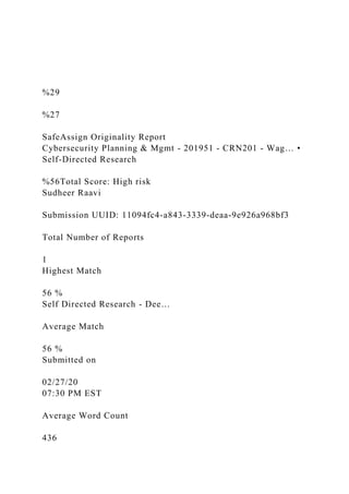
  • 1. %29 %27 SafeAssign Originality Report Cybersecurity Planning & Mgmt - 201951 - CRN201 - Wag… • Self-Directed Research %56Total Score: High risk Sudheer Raavi Submission UUID: 11094fc4-a843-3339-deaa-9e926a968bf3 Total Number of Reports 1 Highest Match 56 % Self Directed Research - Dee… Average Match 56 % Submitted on 02/27/20 07:30 PM EST Average Word Count 436
  • 2. Highest: Self Directed Resear… %56Attachment 1 Institutional database (3) Student paper Student paper Student paper Internet (3) upguard wikipedia airsassociation Top sources (3) Excluded sources (0) View Originality Report - Old Design Word Count: 436 Self Directed Research - Deep and Dark Web.docx 2 6 4 3 1 5 3 upguard 2 Student paper 6 Student paper Source Matches (16) wikipedia 100% Student paper 65% wikipedia 100%
  • 3. Student paper 65% wikipedia 100% wikipedia 100% Student paper 66% Student paper 71% Running head: DEEP WEB VS. DARK WEB 1 DEEP WEB VS. DARK WEB 2 Deep Web vs. Dark Web Name: Sudheer Raavi Institution: New England College Course: Cybersecurity Planning & Mgmt Deep Web vs. Dark Web The deep web and dark web are used interchangeably but have different meanings. The deep web refers to the pages that are not indexed, implying that any search engine will fail to return them after searching. Search engine crawlers cannot see these pages as they are invisible. Deep web, therefore, works in one major way, which is obscurity. Obscurity means the inability to locate an internet resource using any major search engine. The deep web is achieved by adding a preferable robots.txt file to the website (Sen, 2019). It prevents crawlers from indexing such a site and eventually
  • 4. prevents the pages from dis- playing the search engine results pages (SERPS). On the other hand, the dark web refers to the various encrypted overlay and self-contained networks that live on top of the internet and inaccessible unless one has the right protocol and tools. By comparison, the deep web is larger than the dark web. Dark web sites are only in thousands. Usually, the sites in the Dark Web are differentiated by the use of encryption software, which makes any user and the lo- cation secret. It is the reason for illegal activities that are dominant on the dark web because users can hide their identities (Sussman, 2018). The owners of the illegal websites also conceal their location and data transfer occurs anonymously. Overall, the dark web houses various illegal activities like firearms, drug deals, gambling, and other illicit trades. Therefore, the deep web includes various parts of legitimate websites like schools, banks, and other institutional web- sites that require logins. Also, it can be mainstream web like Netflix pages since they are personalized for the users and the URLs are not indexed (Sen, 2019). The dark web, however, is a smaller portion since the sites are intentionally hidden and unreachable through standard search engines. A famous element that offers access to the dark web is the TOR network. TOR network is anonymous and can only access through a specific web browser, known as the TOR browser. Therefore, the dark web has illegal activities due to the anonymity of the TOR network. References Sen, K. (2019). Deep Web vs Dark Web: What's the difference?. Upguard. Retrieved from https://www.upguard.com/blog/dark- web-vs-deep-web
  • 5. Sussman, B. (2018). Dark Web vs. Deep Web: What Is the Difference? Securewrold. Retrived from https://www.secureworldexpo.com/industry- news/dark-web-vs-deep-web 1 2 1 2 1 1 2 2 2 3 4 5 3 6 3 6 1 Student paper DEEP WEB VS. Original source "The Deep Web vs
  • 6. 2 Student paper DARK WEB 1 Original source DEEP WEB 1 1 Student paper DEEP WEB VS. Original source "The Deep Web vs 2 Student paper DARK WEB 2 Original source DEEP WEB 2 1 Student paper Deep Web vs.
  • 7. Original source "The Deep Web vs 1 Student paper Deep Web vs. Original source "The Deep Web vs 2 Student paper The deep web and dark web are used interchangeably but have different meanings. Original source The terms Dark Web and Deep Web can be used interchangeably, but they differ 2 Student paper Obscurity means the inability to locate an internet resource using any major search engine.
  • 8. Original source Obscurity is the inability to locate an in- ternet resource in the search engines Student paper 66% upguard 69% Student paper 67% airsassociation 86% upguard 100% Student paper 100% upguard 100% Student paper 70% 2 Student paper It prevents crawlers from indexing such a site and eventually prevents the pages from displaying the search en- gine results pages (SERPS). Original source Fie to a website, which prevents the search engine crawlers from indexing
  • 9. the site, hence preventing pages dis- playing in the results 3 Student paper On the other hand, the dark web refers to the various encrypted overlay and self-contained networks that live on top of the internet and inaccessible unless one has the right protocol and tools. Original source The dark web refers to any number of self-contained, encrypted overlay net- works that live on top of the internet, inaccessible save for special tools and protocols, hence dark 4 Student paper By comparison, the deep web is larger than the dark web. Original source That is Deep Web and Dark Web 5 Student paper
  • 10. Dark web sites are only in thousands. Original source Dark Web sites number only in the thousands 3 Student paper Deep Web vs Dark Web: What's the difference?. Original source Deep Web vs Dark Web What's the difference 6 Student paper Retrieved from https://www.upguard.- com/blog/dark-web-vs-deep-web Original source Retrieved from https://www.upguard.- com/blog/dark-web-vs-deep-web 3 Student paper Dark Web vs.
  • 11. Original source Dark Web vs 6 Student paper Retrived from https://www.secure- worldexpo.com/industry-news/dark- web-vs-deep-web Original source Retrieved from https://www.upguard.- com/blog/dark-web-vs-deep-web 4 Return and Risk Learning Goals After studying this chapter, you should be able to: 1. LG 1 Review the concept of return, its components, the forces that affect the level of return, and historical returns. 2. LG 2 Discuss the role of the time value of money in measuring return and defining a satisfactory investment. 3. LG 3 Describe real, risk-free, and required returns and the calculation and application of holding period return. 4. LG 4 Explain the concept and the calculation of an internal rate of return and how to find growth rates. 5. LG 5 Discuss the key sources of risk that might affect potential investments. 6. LG 6 Understand the risk of a single asset, risk assessment, and the steps that combine return and risk. An old saying often attributed to Mark Twain advises, “Buy
  • 12. land—they’re not making it anymore.” That bit of folk wisdom gained enormous popularity during the U.S. real estate boom. According to the S&P/Case-Shiller Index, which tracks home prices in 20 large cities, U.S. homeowners saw their property values increase more than 100% from 2000 to 2005. Over the same six years, the U.S. stock market (as measured by the S&P 500 Index) lost more than 10% of its value. Moreover, the tantalizing returns on real estate seemed to come without much risk. The average home price rose every single month from July 1996 to May 2006. No wonder, then, that investing in real estate became fashionable, as evidenced by the introduction of television shows such as A&E’s Flip This House. It seemed that no one could lose money by investing in residential real estate. Unfortunately, home prices began to decline in late summer 2006, and their fall continued through March 2012. Over that period, average home prices dropped 34% and millions of properties were lost to foreclosure, reminding homeowners that investing in real estate has both rewards and risks. After hitting bottom in March 2012 the S&P/Case-Shiller Index rose 29% by the end of 2014; however, this rebound lagged behind the S&P 500 Index return of 46% over the same period. The boom and bust cycles in both the housing and stock markets over the last decade provide great examples of the almost inextricable link between risk and return. Some investments may deliver high returns for several consecutive years, just as housing did in the mid 2000s, but high returns tend to be associated with high risks, as investors in housing learned after 2006. This chapter and the next discuss tools that will help you quantify the tradeoff between risk and return. (Source: S&P/Case-Shiller price indexes downloaded from http://www .standardandpoors.com and http://www.realtytrac.com/, “Year- End 2014 U.S. Foreclosure Market Report.”) The Concept of Return 1. LG 1
  • 13. 2. LG 2 People are motivated to invest in a given asset by its expected return. The return is the level of profit from an investment—that is, the reward for investing. Suppose you have $1,000 in an insured savings account paying 2% annual interest, and a business associate asks you to lend her that much money. If you lend her the money for one year, at the end of which she pays you back, your return will depend on the amount of interest you charge. If you make an interest-free loan, your return will be 0. If you charge 2% interest, your return will be $20 (0.02 × $1,000). Because you are already earning a safe 2% on the $1,000, it seems clear that to equal that return you should charge your associate a minimum of 2% interest. Some investments guarantee a return, but most do not. The return on a bank deposit insured by the federal government is virtually certain. The return earned on a loan to your business associate might be less certain. The size and the certainty of the expected return are important factors in choosing a suitable investment. Components of Return The return on an investment comes from two sources. One source is periodic payments, such as dividends and interest. The other source is the change in the investment’s price. We call these two components of an investment’s return current income and capital gains (or capital losses), respectively. Income Income may take the form of dividends from stocks or mutual funds or interest received on bonds. For our purposes, an investment’s income is the cash that investors periodically receive as a result of owning the investment. Investor Facts Burrito Bonds are Easy to Swallow In the summer of 2014, the London-based restaurant chain, Chilango, sold bonds to investors that promised cash interest payments of 8% per year, plus vouchers for free burritos. Though those burritos undoubtedly have some value to Chilango’s investors, when we
  • 14. calculate an investment’s return, we’ll focus on the cash payments that the investment makes, ignoring any in-kind payments like free burritos. (Source: “Will Chilango’s £2m Success Herald an Affordable Mini Bond Revolution?” http://www.forbes.com/sites/trevorclawson/2014/0 8/28/will-chilangos-2m-success-herald-an-affordable-mini- bond-revolution/, accessed April 23, 2015.) Using the data in Table 4.1, we can calculate the income from investments A and B, both purchased for $1,000, over a one- year period of ownership. Investment A provides income of $80, and investment B pays $120. Solely on the basis of the income received over the one year, investment B seems preferable. Capital Gains (or Losses) The second dimension of return focuses on the change in an investment’s market value. As noted in Chapter 1, the amount by which the proceeds from the sale of an investment exceed its original purchase price is a capital gain. If an investment sells for less than its original purchase price, a capital loss results. Table 4.1 Profiles of Two Investments Investment A B Purchase price (beginning of year) $1,000 $1,000 Cash received 1st quarter $ 10 $ 0 2nd quarter $ 20
  • 15. $ 0 3rd quarter $ 20 $ 0 4th quarter $ 30 $ 120 Total income (for year) $ 80 $ 120 Sale price (end of year) $1,100 $ 960 Table 4.2 Total Returns of Two Investments Investment Return A B Income $ 80 $120 Capital gain (loss) $100 $(40) Total return $180 $ 80 We can calculate the capital gain or loss of the investments shown in Table 4.1. Investment A experiences a capital gain of $100 ($1,100 sale price −$1,000 purchase price) over the one- year period. Investment B, on the other hand, earned a $40 capital loss ($960 sale price − $1,000 purchase price). Combining the capital gain (or loss) with the income (calculated in the preceding section) gives the total return. Table 4.2 shows the total return for investments A and B over the year.
  • 16. Investment A earns a $180 total return, compared to just $80 earned by investment B. It is generally preferable to use percentage returns rather than dollar returns. Percentages allow direct comparison of different sizes and types of investments. Investment A earned an 18% return ($180 , $1,000); B produced only an 8% return ($80 , $1,000). At this point investment A appears preferable, but as we’ll see, differences in risk might cause some investors to prefer B. Watch Your Behavior Investment Club’s Returns Less Than Advertised In the mid 1990s, an investment club known as the Beardstown Ladies gained notoriety, at first because they claimed to have earned higher returns than the overall stock market for more than a decade. The ladies wrote a best-selling book full of investment advice, but no where in that book did they discuss how to calculate an investment’s return. An audit later revealed that the Beardstown ladies grossly overstated their returns by including new capital investments as part of their return. After this error was corrected, the investment’s club trailed the broader stock market by several percentage points. Knowing how to calculate returns properly is the first step in assessing an investment’s performance. Source: “Where Are They Now: The Beardstown Ladies,” http://www.wsj .com/articles/SB114596682916135186, accessed June 29, 2016. Why Return Is Important An asset’s return is a key variable in the investment decision because it indicates how rapidly an investor can build wealth. Naturally, because most people prefer to have more wealth rather than less, they prefer investments that offer high returns rather than low returns if all else is equal. However, we’ve already said that the returns on most investments are uncertain, so how do investors distinguish assets that offer high returns from those likely to produce low returns? One way to make this kind of assessment is to examine the returns that different types
  • 17. of investments have produced in the past. Historical Performance Most people recognize that future performance is not guaranteed by past performance, but past data often provide a meaningful basis for future expectations. A common practice in the investment world is to look closely at the historical record when formulating expectations about the future. Consider the data for ExxonMobil Corporation presented in Table 4.3. ExxonMobil paid dividends every year from 2005 through 2014. ExxonMobil’s stock price generally rose during this decade, starting at $51.26 and ending at $92.45. Despite the overall upward trend, the company’s stock price fell in 2008 and 2009 (largely due to the Great Recession and the corresponding drop in oil prices), and it declined again in 2014 (largely due to a rapid increase in the supply of oil and shrinking worldwide demand for oil). Two aspects of these data are important. First, we can determine the annual total return generated by this investment over the past 10 years. The average annual total return earned by ExxonMobil’s shareholders (column 6) over this period was 9.6%, performance that put ExxonMobil ahead of Table 4.3 Historical Investment Data for Exxonmobil Corp. (XOM) (Source: Dividends and end-of-year closing prices were obtained from Yahoo! Finance.) Market Value (Price) Yearly Total Return Year (1) Dividend Income (2) Beginning of Year (3) End of Year (4) (3) − (2) Capital Gain (5) (1) + (4) (6) (5) / (2) 2005
  • 18. $1.14 $ 51.26 $ 56.17 $ 4.91 $ 6.05 11.8% 2006 $1.28 $ 56.17 $ 76.63 $20.46 $ 21.74 38.7% 2007 $1.37 $ 76.63 $ 93.69 $ 17.06 $18.43 24.1% 2008 $1.55 $ 93.69 $ 79.83 −$13.86 −$ 12.31 −13.1% 2009 $1.66 $ 79.83 $ 68.19 −$ 11.64 −$ 9.98 −12.5% 2010 $1.74
  • 19. $ 68.19 $ 73.12 $ 4.93 $ 6.67 9.8% 2011 $1.85 $ 73.12 $ 84.76 $ 11.64 $ 13.49 18.4% 2012 $2.18 $ 84.76 $ 86.55 $ 1.79 $ 3.97 4.7% 2013 $2.46 $ 86.55 $101.20 $14.65 $ 17.11 19.8% 2014 $2.70 $101.20 $ 92.45 −$ 8.75 −$ 6.05 −6.0% Average $1.79
  • 20. $ 4.12 $ 5.91 9.6% many other stocks for the same period. Second, observe that there was considerable variation in ExxonMobil’s return from one year to the next. The firm’s best year was 2006, during which its investors earned a total return of 38.7%. But in 2008, ExxonMobil’s worst year, shareholders lost 13.1%. [email protected] Expected Return In the final analysis, of course, it’s the future that matters when we make investment decisions. Therefore an investment’s expected return is a vital measure of its performance. It’s what you think the investment will earn in the future that determines what you should be willing to pay for it. To demonstrate, let’s return to the data in Table 4.3. A naive investor might estimate ExxonMobil’s expected return to be the same as its average return from the prior decade, 9.6%. That’s not necessarily a bad starting point, but it would be wise to ask, “What contributed to ExxonMobil’s past returns, and is it likely that the same factors will occur in the future?” Central to ExxonMobil’s success in the recent past was a generally upward trend in oil prices. In early 2005, crude oil traded for around $58 per barrel, but prices rose steadily until they peaked around $140 per barrel in June 2008. Even though prices fell sharply for a brief period during the recession, the price of oil did not fall below $70 at any point from June 2009 to October 2014, so this was a very favorable period for ExxonMobil. This suggests that the historical returns shown in Table 4.3 might represent a better-than-average period for the company. An investor who believed that oil prices would not continue to move up indefinitely, but rather would stabilize, might estimate ExxonMobil’s expected return by looking at its historical performance during a period of relatively stable oil prices. Level of Return
  • 21. The level of return achieved or expected from an investment will depend on a variety of factors. The key factors are internal characteristics and external forces. Famous Failures in Finance Fears of Deflation Worry Investors For most of your lifetime, prices of most goods and services have been rising. There are important exceptions, such as the prices of consumer electronics and computers, but from one year to the next, the overall price level rose continuously in the United States from 1955 through 2007. However, as the recession deepened in 2008, consumer prices in the United States began to decline, falling in each of the last five months that year. Countries in the European Union experienced a brief deflationary period around the same time. The news raised fears among some investors that the recession might turn into a depression like the one that had brought about a price decline of -27% from November 1929 to March 1933. Although prices began to rise again, fears of deflation resurfaced again in late 2014 and early 2015. Prices in the United States were flat or down in the first three months of 2015, while countries in the European Union experienced falling prices for four consecutive months starting in December 2015. Critical Thinking Question 1. Suppose you own an investment that pays a fixed return in dollars year after year. How do you think inflation (rising prices) or deflation (falling prices) would influence the value of this type of investment? Internal Characteristics Certain characteristics of an investment affect its return. For investments issued by companies, the important characteristics include things such as the type of investment (e.g., stocks or bonds), the quality of the firm’s management, and whether the firm finances its operations with debt or equity. For example, investors might expect a different return on the common stock of a large, well-managed, completely equity-financed plastics manufacturer than they would anticipate from the common stock of a small, poorly managed, largely debt-financed clothing
  • 22. manufacturer. As we will see in later chapters, assessing internal factors and their impact on return is one important step in analyzing possible investments. External Forces External forces such as Federal Reserve actions, recessions, wars, and political events may also affect an investment’s return. None of these are under the control of the issuer of the investment, and investments react differently to these forces. For example, if investors expect oil prices to rise, they may raise their expected return for ExxonMobil stock and lower it for the stock of an automobile manufacturer that produces gas guzzlers. Likewise, the economies of various countries respond to external forces in different ways. What Is Inflation? Another external force is the general level of price changes, either up—inflation—or down—deflation. How inflation (or deflation) affects investment returns is complex, but it depends in part on whether investors correctly anticipate the rate of inflation. Generally speaking, when investors expect inflation to occur, they will demand higher returns. For example, when we look back through history, we see that interest rates on bonds were usually higher in periods when inflation was higher. However, when investors are caught off guard and the rate of inflation is higher or lower than they expected, returns on investments may rise or fall in response. The way that investment returns respond to unexpected changes in inflation will vary from one type of investment to another, and that response can be influenced by investors’ beliefs about how policymakers will react to changing inflation. For example, if inflation unexpectedly rises, investors might anticipate that the Federal Reserve will take action to slow economic growth to bring inflation back down. In that case, returns on some investments might fall even as inflation is accelerating. Table 4.4 Historical Returns for Major Asset Classes (1900– 2014)
  • 23. (Source: Credit Suisse Global Investment Returns Yearbook 2015.) Average Annual Return Stocks Long-Term Government Bonds Short-Term Government Bills Inflation Australia 11.4% 5.6% 4.5% 3.8% Belgium 7.9% 5.5% 4.8% 5.1% Canada 8.9% 5.3% 4.5% 3.0% Denmark 9.3% 7.2% 6.0% 3.8% Finland 12.9% 7.3% 6.6% 7.1% France
  • 25. 5.6% 4.8% 3.7% South Africa 12.7% 6.9% 6.0% 4.9% Spain 9.5% 7.6% 6.0% 5.7% Sweden 9.4% 6.3% 5.3% 3.4% Switzerland 6.8% 4.6% 3.0% 2.2% United Kingdom 9.4% 5.5% 4.8% 3.9% United States 9.6% 5.0% 3.8% 2.9% Historical Returns Returns vary both over time and among types of investments. By averaging historical yearly returns over a long period of
  • 26. time, it is possible to observe the differences in annual returns earned by various types of investments. Table 4.4 shows the average annual rates of return for three major asset classes (stocks, treasury bonds, and treasury bills) in 19 countries over the 115-year period from 1900 to 2014. With more than 100 years of data to draw on, some clear patterns emerge. You can see that significant differences exist among the average annual rates of return realized on stocks, long-term government bonds, and short-term government bills. In all 19 countries, stocks earn higher returns than government bonds, which in turn earn higher average returns than short-term government bills. Later in this chapter, we will see how we can link these differences in return to differences in the risk of each of these investments. We now turn our attention to the role that time value of money principles play in determining investment returns. The Time Value of Money and Returns The phrase the time value of money refers to the fact that it is generally better to receive cash sooner rather than later. For example, consider two investments, A and B. Investment A will pay you $100 next year and $100 the year after that. Investment B pays you $200 in two years. Assume that neither investment has any risk, meaning that you are certain that you will receive these cash payments. Clearly both investments pay $200 over two years, but investment A is preferable because you can reinvest the $100 you receive in the first year to earn more interest the second year. You should always consider time value of money principles when making investment decisions. An Advisor’s Perspective Ed Slott CEO, Ed Slott and Company “The greatest money making asset any individual can possess is time.” MyFinanceLab We now review the key computational aids for streamlining time value of money calculations, and then we demonstrate the application of time value of money techniques to determine an
  • 27. acceptable investment. Computational Aids for Use in Time Value of Money Calculations The once time-consuming calculations involved in applying time value of money techniques can be simplified with a number of computational aids. Throughout this text we will demonstrate the use of hand-held financial calculators and electronic spreadsheets. Financial calculators include numerous preprogrammed financial routines. To demonstrate the calculator keystrokes for various financial computations, we show a keypad, with the keys defined below. Electronic spreadsheet use has become a prime skill for today’s investors. Like financial calculators, spreadsheets have built-in routines that simplify time value of money calculations. For most time value of money calculations in the text, we show spreadsheet solutions with clearly identified cell entries. Determining a Satisfactory Investment You can use time value of money techniques to determine whether an investment’s return is satisfactory given the investment’s cost. Ignoring risk at this point, a satisfactory investment would be one for which the present value of benefits (discounted at the appropriate discount rate) equals or exceeds its cost. The three possible cost–benefit relationships and their interpretations follow: 1. If the present value of the benefits equals the cost, you would earn a rate of return equal to the discount rate. 2. If the present value of benefits exceeds the cost, you would earn a rate of return greater than the discount rate. 3. If the present value of benefits is less than the cost, you would earn a rate of return less than the discount rate. You would prefer only those investments for which the present value of benefits equals or exceeds its cost—situations 1 and 2. In these cases, the rate of return would be equal to or greater than the discount rate. [email protected]
  • 28. Table 4.5 Present Value Applied to An Investment End of Year (1) Income (2) Present Value Calculation at 8% (3) Present Value at 8% 1 $ 90 $ 90/(1.08)1 $ 83.33 2 $ 100 $ 100/(1.08)2 $ 85.73 3 $ 110 $ 110/(1.08)3 $ 87.32 4 $ 120 $ 120/(1.08)4 $ 88.20 5 $ 100 $ 100/(1.08)5 $ 68.06 6 $ 100 $ 100/(1.08)6 $ 63.02 7 $1,200 $1,200/(1.08)7 $ 700.19 Total Present Value
  • 29. $1,175.85 Time Is Money The information in Table 4.5 demonstrates the application of present value to investment decision making. (Note: You can use a financial calculator or an Excel spreadsheet to convert the algebraic expression in column 2 to the numeric value in column 3.) This investment makes a series of payments over the next seven years. Because the payments arrive at different times, we calculate the present value of each payment to determine how much each payment is worth in today’s dollars. The present value of the benefits (i.e., the income) provided by this investment over its seven-year life is $1,175.85. If the cost of the investment today is $1,175.85 or less, then the investment is acceptable. At that cost, an investor would earn a rate of return equal to at least 8%. At a cost above the $1,175.85 present value, the investment would not be acceptable because the rate of return would be less than 8%. In that case it would be preferable to find an alternative investment with a present value of benefits that equals or exceeds its cost. For your convenience, Appendix 4A provides a complete review of the key time value of money techniques. Be sure to review it before reading ahead, to make sure you have adequate understanding of this important financial concept. Concepts in Review Answers available at http://www.pearsonhighered.com/smart 1. 4.1 Explain what is meant by the return on an investment. Differentiate between the two components of return—income and capital gains (or losses). 2. 4.2 What role do historical performance data play in estimating an investment’s expected return? Discuss the key factors affecting investment returns—internal characteristics and external forces. 3. 4.3 What is a satisfactory investment? When the present value of benefits exceeds the cost of an investment, what can you conclude about the rate of return earned by the investor
  • 30. relative to the discount rate? Measuring Return 1. LG 3 2. LG 4 Thus far, we have discussed the concept of return in terms of its two components (income and capital gains) and the key factors that affect the level of return (internal characteristics and external forces). These discussions intentionally oversimplified the computations involved in determining the historical or expected return. To compare returns from different investments, we need to incorporate time value of money concepts that explicitly consider differences in the timing of investment income and capital gains. We must also be able to calculate the present value of future benefits. Here we will look at several measures that enable us to compare alternative investments. First, we must define and consider the relationships among various rates of return. Real, Risk-Free, and Required Returns Inflation and Returns Glance back at Table 4.4, which reports that in the United States the average annual return on a short-term government Treasury bill was 3.8% between 1900 and 2014. The table also shows that the average annual inflation rate was 2.9%. It’s no coincidence that the T-bill rate of return exceeds the inflation rate because investors want to earn returns that exceed the inflation rate. Inflation erodes the purchasing power of money. For example, if prices of most goods and services rise by 3% in a year, $1 buys about 3% fewer goods and services at the end of the year than at the beginning. Thus, if investors seek to increase their purchasing power over time, they must earn returns that exceed the inflation rate. The nominal rate of return on an investment is the return that the investment earns expressed in current dollars. For example, if you put $50 into an investment that promises to pay 3% interest, at the end of the year you will have $51.50 (the initial $50 plus a $1.50 return). Your nominal return is 3%, but this
  • 31. does not necessarily mean that you are better off financially at the end of the year because the nominal return does not take into account the effects of inflation. To continue the example, assume that at the beginning of the year, one bag of groceries costs $50. During the year, suppose grocery prices rise by 3%. This means that by the end of the year one bag of groceries costs $51.50. In other words, at the beginning of the year you could have used your $50 either to buy one bag of groceries or to make the investment that promised a 3% return. If you invested your money rather than spending it on groceries, by the end of the year you would have had $51.50, still just enough to buy one bag of groceries. In other words, your purchasing power did not increase at all during the year. The real rate of return on an investment measures the increase in purchasing power that the investment provides. In our continuing example, the real rate of return is 0% even though the nominal rate of return is 3%. In dollar terms, by investing $50 you increased your wealth by 3% to $51.50, but in terms of purchasing power you are no better off because you can only buy the same amount of goods that you could have bought before you made the investment. In mathematical terms, the real rate of return is approximately equal to the nominal rate of return minus the inflation rate. Example Suppose you have $50 today and are trying to decide whether to invest that money or spend it. If you invest it, you believe that you can earn a nominal return of 10%, so after one year your money will grow to $55. If you spend the money today, you plan to feed your caffeine habit by purchasing 20 lattes at your favorite coffee shop at $2.50 each. You decide to save and invest your money, so a year later you have $55. How many more lattes can you buy because you chose to invest your money rather than spend it right away? Unfortunately, during the year inflation caused the price of a latte to increase by 4.8% from $2.50 to $2.62. At the new price, you can just about afford to buy 21 lattes (21 × $2.62 = $55.02). That extra latte
  • 32. represents an increase in your purchasing power of 5% (i.e., 21 is 5% more than 20), so your real return on the investment is 5% because it enabled you to buy 5% more than you could before you invested. Notice that the real return is approximately equal to the difference between the investment’s nominal return (10%) and the inflation rate (4.8%): Real return≈Nominal return−Inflation rate5%≈10%−4.8%Real return≈Nominal return −Inflation rate5%≈10%−4.8% Risk and Returns Investors are generally risk averse, meaning that they do not like risk and will only take … 5 Modern Portfolio Concepts Learning Goals After studying this chapter, you should be able to: 1. LG 1 Understand portfolio objectives and the procedures used to calculate portfolio return and standard deviation. 2. LG 2 Discuss the concepts of correlation and diversification and the key aspects of international diversification. 3. LG 3 Describe the components of risk and the use of beta to measure risk. 4. LG 4 Explain the capital asset pricing model (CAPM) conceptually, mathematically, and graphically. 5. LG 5 Review the traditional and modern approaches to portfolio management. 6. LG 6 Describe portfolio betas, the risk-return tradeoff, and reconciliation of the two approaches to portfolio management. United Rentals Inc. (URI) rents construction and industrial equipment to contractors, businesses, governments, and individuals. The company specializes in heavy equipment such as earth-moving machines and forklifts. During the recession that began in 2007, many companies found that they did not have enough work to do to keep the machines they already owned running, so naturally the demand for rental equipment suffered. URI stock reached a 2007 peak of over $35 per share
  • 33. in May, but after that began a long slide, hitting bottom at $2.52 in March 2009. That spring, the economy began to show signs of life, and URI stock surged, rising nearly 200% from its low point by August 2009. Heiko Ihle, a stock analyst for the Gabelli & Co. money management firm, issued a “buy” rating on URI despite the fact that the company had high leverage (meaning that it borrowed a lot of money to finance its operations). Ihle noted that URI stock had a high beta, meaning that it moved sharply when the broader market shifted. Mr. Ihle’s recommendation proved to be a good one. From the end of August 2009 to the end of August 2014, the value of URI stock climbed almost 1,200% and was trading above $119 per share. Over that same period of time, the S&P 500 Index, a widely used indicator of the overall stock market, rose by a less dramatic 95%. In this chapter we continue to explore the tradeoff between risk and return, and we’ll see that a stock’s beta—its sensitivity to movements in the overall stock market—has a big effect on both the stock’s risk and the return that it offers investors. (Sources: Yahoo! Finance; “U.S. Hot Stocks: Legg Mason, JDA Software Active in Late Trading,” July 20, 2009; The Wall Street Journal Digital Network, http://online.wsj.com/article/BT-CO-20090720- 713541.html.) Principles of Portfolio Planning 1. LG 1 2. LG 2 Investors benefit from holding portfolios of investments rather than single investments. Without necessarily sacrificing returns, investors who hold portfolios can reduce risk. Surprisingly, the volatility of a portfolio may be less than the volatilities of the individual assets that make up the portfolio. In other words, when it comes to portfolios and risk, the whole is less than the sum of its parts! A portfolio is a collection of investments assembled to meet one
  • 34. or more investment goals. Of course, different investors have different objectives for their portfolios. The primary goal of a growth-oriented portfolio is long-term price appreciation. An income-oriented portfolio is designed to produce regular dividends and interest payments. Portfolio Objectives Setting portfolio objectives involves definite tradeoffs, such as the tradeoff between risk and return or between potential price appreciation and income. How investors evaluate these tradeoffs will depend on their tax bracket, current income needs, and ability to bear risk. The key point is that portfolio objectives must be established before one begins to invest. The ultimate goal of an investor is an efficient portfolio, one that provides the highest return for a given risk level. Efficient portfolios aren’t necessarily easy to identify. Investors usually must search out investment alternatives to get the best combinations of risk and return. Portfolio Return and Standard Deviation The first step in forming a portfolio is to analyze the characteristics of the securities that an investor might include in the portfolio. Two of the most important characteristics to examine are the returns that each asset might be expected to earn and the uncertainty surrounding that expected return. As a starting point, we will examine historical data to see what returns stocks have earned in the past and how much those returns have fluctuated to get a feel for what the future might hold. The portfolio return is calculated as a weighted average of returns on the assets (i.e., the investments) that make up the portfolio. You can calculate the portfolio return, rp, by using Equation 5.1. The portfolio return depends on the returns of each asset in the portfolio and on the fraction invested in each asset, wj. PortfolioReturn=(Proportion of portfolios totaldollar valueinvested inasset 1×Returnon asset1)+(Proportion of portfolio's totaldollar valueinvested inasset 2×Returnon
  • 35. asset2)+...+(Proportion ofportfolio's totaldollar valueinvested inassetn×Returnon assetn)=n∑j=1(Proportion of portfolio's totaldollar valueinvested inassetj×Returnon assetj)Portfolio Return=(Proportion of portfolios total dollar value invested in asset 1×Return on asset 1)+(Proportion of portfolio's total dollar value invested in asset 2×Return on asset 2)+...+(Proportion of portfolio's total dollar value invested in asset n×Return on asset n)=∑j=1n(Proportion of portfolio's total dollar value invested in asset j×Return on asset j)Equation5.1 rp=(w1×r1)+(w2×r2)+...+(wn×rn)=n∑j=1(wj×rj)rp=(w1×r1)+(w 2×r2)+...+(wn×rn)=∑j=1n(wj×rj)Equation5.1a The fraction invested in each asset, wj, is also known as a portfolio weight because it indicates the weight that each asset receives in the portfolio. Of course, n∑j=1wj=1∑j=1nwj=1, which means that the sum of the portfolio weights must equal 100%. In other words, when you add up the fractions invested in all of the assets, that sum must equal 1.0. Panel A of Table 5.1 shows the historical annual returns on two stocks, International Business Machines Corp. (IBM) and Celgene Corp. (CELG), from 2005 through 2014. Over that period, IBM earned an average annual return of 9.0%, which is close to the average annual return on the U.S. stock market during the past century. In contrast, Celgene Corp. earned a spectacular 40.7% average annual return. Although Celgene may not repeat that kind of performance over the next decade, it is still instructive to examine the historical figures. [email protected] Table 5.1 Individual And Portfolio Returns And Standard Deviation Of Returns For International Business Machines (Ibm) And Celgene (Celg) Source: End-of-year closing prices are obtained from Yahoo Finance and are adjusted for dividends and stock splits. A. Individual and Portfolio Returns (1)
  • 36. (2) (3) (4) Historical Returns* Portfolio Weights Portfolio Return Year (t) rIBM% rCELG% WIBM = 0.86 WCELG = 0.14 rp% 2005 −15.8% 144.3% (0.86 × -15.8%) + (0.14 × 144.3%) = 6.6% 2006 19.8% 77.5% (0.86 × 19.8%) + (0.14 × 77.5%) = 27.9% 2007 12.8% −19.7% (0.86 × 12.8%) + (0.14 × -19.7%) = 8.3% 2008 −20.8% 19.7% (0.86 × -20.8%) + (0.14 × 19.7%) = −15.1% 2009 58.6% 0.7%
  • 37. (0.86 × 58.6%) + (0.14 × 0.7%) = 50.5% 2010 14.3% 6.2% (0.86 × 14.3%) + (0.14 × 6.2%) = 13.1% 2011 27.4% 14.3% (0.86 × 27.4%) + (0.14 × 14.3%) = 25.6% 2012 5.9% 16.1% (0.86 × 5.9%) + (0.14 × 16.1%) = 7.3% 2013 −0.2% 115.3% (0.86 × -0.2%) + (0.14 × 115.3%) = 16.0% 2014 −12.4% 32.4% (0.86 × -12.4%) + (0.14 × 32.4%) = −6.1% Average Return 9.0% 40.7% 13.4% B. Individual and Portfolio Standard Deviations Standard Deviation Calculation for IBM:
  • 38. ⎷ 10∑t=1(rt−¯r)2n−1=√(−15.8%−9.0%)2+...+(−12.4%−9.0%)2 10−1=√5015.4%210−1=23.6%SIBM=∑t=110(rt−r¯)2n−1=(−15.8 %−9.0%)2+...+(−12.4%−9.0%)210−1=5015.4%210−1=23.6% Standard Deviation Calculation for CELG: ⎷ 10∑t=1(rt−¯r)2n−1=√(144.3%−40.7%)2+...+(32.4%−40.7%) 210−1=√2,5913.3%210−1=53.7%SCELG=∑t=110(rt−r¯)2n−1=( 144.3%−40.7%)2+...+(32.4%−40.7%)210−1=2,5913.3%210−1=5 3.7% Standard Deviation Calculation for Portfolio: ⎷ 10∑t=1(rt−¯r)2n−1=√(6.6%−13.4%)2+...+(−6.1%−13.4%)21 0−1=√3045.8%210−1=18.4%SP=∑t=110(rt−r¯)2n−1=(6.6%−13. 4%)2+...+(−6.1%−13.4%)210−1=3045.8%210−1=18.4% *Annual rate of return is calculated based on end-of-year closing prices. Suppose we want to calculate the return on a portfolio containing investments in both IBM and Celgene. The first step in that calculation is to determine how much of each stock to hold. In other words, we must to decide what weight each stock should receive in the portfolio. Let’s assume that we want to invest 86% of our money in IBM and 14% in CELG. What kind of return would such a portfolio earn? We know that over this period, Celgene earned much higher returns than IBM, so intuitively we might expect that a portfolio containing both stocks would earn a return higher than IBM’s but lower than Celgene’s. Furthermore, because most (86%) of the portfolio is invested in IBM, you might guess that the portfolio’s return would be closer to IBM’s than to Celgene’s. Columns 3 and 4 in Panel A show the portfolio’s return each
  • 39. year. The average annual return on this portfolio was 13.4% and as expected it is higher than the return on IBM and lower than the return on Celgene. By investing a little in Celgene, an investor could earn a higher return than would be possible by holding IBM stock in isolation. What about the portfolio’s risk? To examine the risk of this portfolio, starting by measuring the risk of the stocks in the portfolio. Recall that one measure of an investment’s risk is the standard deviation of its returns. Panel B of Table 5.1 applies the formula for standard deviation that we introduced earlier to calculate the standard deviation of returns on IBM and Celgene stock. Or, if you prefer, rather than using the formulas in Table 5.1 to find the standard deviation of returns for IBM and CELG, you can construct an Excel spreadsheet to do the calculations, as shown below. The standard deviation of IBM’s returns is 23.6%, and for Celgene’s stock returns the standard deviation is 53.7%. Here again we see evidence of the tradeoff between risk and return. Celgene’s stock earned much higher returns than IBM’s stock, but Celgene returns fluctuate a great deal more as well. Because Celgene’s returns are more volatile than IBM’s, you might expect that a portfolio containing both stocks would have a standard deviation that is higher than IBM’s but lower than Celgene’s. In fact, that’s not what happens. The final calculation in Panel B inserts the IBM-Celgene portfolio return data from column 4 in Panel A into the standard deviation formula to calculate the portfolio’s standard deviation. Panel B shows the surprising result that the portfolio’s returns are less volatile than are the returns of either stock in the portfolio! The portfolio’s standard deviation is just 18.4%. This is great news for investors. An investor who held only IBM shares would have earned an average return of only 9.0%, but to achieve that return the investor would have had to endure IBM’s 23.6% standard deviation. By selling a few IBM shares and using the proceeds to buy a few Celgene shares (resulting in the 0.86 and
  • 40. 0.14 portfolio weights shown in Table 5.1), an investor could have simultaneously increased his or her return to 13.4% and reduced the standard deviation to 18.4%. In other words, the investor could have had more return and less risk at the same time. This means that an investor who owns nothing but IBM shares holds an inefficient portfolio—an alternative portfolio exists that has a better return-to-risk tradeoff. That’s the power of diversification. Next, we will see that the key factor in making this possible is a low correlation between IBM and Celgene returns. Correlation and Diversification Diversification involves the inclusion of a number of different investments in a portfolio, and it is an important aspect of creating an efficient portfolio. Underlying the intuitive appeal of diversification is the statistical concept of correlation. Effective portfolio planning requires an understanding of how correlation and diversification influence a portfolio’s risk. Correlation Correlation is a statistical measure of the relationship between two series of numbers. If two series tend to move in the same direction, they are positively correlated. For instance, if each day we record the number of hours of sunshine and the average daily temperature, we would expect those two series to display positive correlation. Days with more sunshine tend to be days with higher temperatures. If the series tend to move in opposite directions, they are negatively correlated. For example, if each day we record the number of hours of sunshine and the amount of rainfall, we would expect those two series to display negative correlation because, on average, rainfall is lower on days with lots of sunshine. Finally, if two series bear no relationship to each other, then they are uncorrelated. For example, we would probably expect no correlation between the number of hours of sunshine on a particular day and the change in the value of the U.S. dollar against other world currencies on the same day. There is no obvious connection between sunshine and world currency markets.
  • 41. The degree of correlation—whether positive or negative—is measured by the correlation coefficient, which is usually represented by the Greek symbol rho (r). It’s easy to use Excel to calculate the correlation coefficient between IBM and Celgene stock returns, as shown in the following spreadsheet. Excel will quickly tell you that the correlation coefficient between IBM and Celgene during the 2005–2014 period was - 0.43. The negative figure means that there was a tendency over this period for the two stocks to move in opposite directions. In other words, years in which IBM’s return was better than average tended to be years in which Celgene’s returns was worse than average, and vice versa. A negative correlation between two stocks is somewhat unusual because most stocks are affected in the same way by large, macroeconomic forces. In other words, most stocks tend to move in the same direction as the overall economy, which means that most stocks will display at least some positive correlation with each other. Because IBM is a major provider of information technology services and Celgene is a biopharmaceutical manufacturer, it is not too surprising that the correlation between these two stocks is not strongly positive. The companies compete in entirely different industries, have different customers and suppliers, and operate within very different regulatory constraints; however, the relatively large (-0.43) magnitude of their negative correlation raises concerns and should cause us to question the validity of basing investment decisions on this correlation measure. Perhaps the sample period we are using to estimate this correlation is too short or is not truly representative of the investment performance of these two stocks. The 2005 to 2014 period that we are focusing on consists of just 10 yearly return observations, and during this particular period there were no fewer than three strong systematic market-wide events (i.e., a financial crisis, a Great Recession, and an economic recovery). Those sharp macroeconomic fluctuations tended to drive most securities’ returns up and down at the same time, which in turn
  • 42. leads to a positive correlation between most pairs of stocks, even when those stocks are drawn from different industries. Ten yearly observations is without question a small sample size, and it may be too small, at least in this case, to accurately capture a meaningful measure of correlation between IBM and Celgene. One way to address this concern is to increase the period of time over which the correlation is being measured and in this way increase the number of yearly observations. Alternatively, one could use monthly returns over the same 10-year period, thereby increasing the number of observations by a factor of 12. What’s the Correlation? For any pair of investments that we might want to study, the correlation coefficient ranges from +1.0 for perfectly positively correlated series to −1.0 for perfectly negatively correlated series. Figure 5.1 illustrates these two extremes for two pairs of Figure 5.1 The Correlations of Returns between Investments M and P and Investments M and N. Investments M and P produce returns that are perfectly positively correlated and move exactly together. On the other hand, returns on investments M and N move in exactly opposite directions and are perfectly negatively correlated. In most cases, the correlation between any two investments will fall between these two extremes. investments: M and P, and M and N. M and P represent the returns on two investments that move perfectly in sync, so they are perfectly positively correlated. In the real world it is extremely rare to find two investments that are perfectly correlated like this, but you could think of M and P as representing two companies that operate in the same industry, or even two mutual funds that invest in the same types of stocks. In contrast, returns on investments M and N move in exactly opposite directions and are perfectly negatively correlated. While these two extreme cases can be illustrative,
  • 43. the correlations between most asset returns exhibit some degree (ranging from high to low) of positive correlation. Negative correlation is the exception. Diversification As a general rule, the lower the correlation between any two assets, the greater the risk reduction that investors can achieve by combining those assets in a portfolio. Figure 5.2 shows negatively correlated assets F and G, both having the same average return, ¯rr¯. The portfolio that contains both F and G has the same return, ¯rr¯, but has less risk (variability) than either of the individual assets because some of the fluctuations in asset F cancel out fluctuations in G. As a result, the combination of F and G is less volatile than either F or G alone. Even if assets are not negatively correlated, the lower the positive correlation between them, the lower the resulting risk. Table 5.2 shows the average return and the standard deviation of returns for many combinations of IBM and Celgene stock. Columns 1 and 2 show the percentage of the portfolio invested in IBM and Celgene, respectively, and columns 3 and 4 show the portfolio average return and standard deviation. Notice that as you move from the top of the table to the bottom (i.e., from investing the entire portfolio in IBM to investing all of it in Celgene), the portfolio return goes up. That makes sense because as you move from top to bottom, the percentage invested in Celgene increases, and Celgene’s average return is higher than IBM’s. The general conclusion from column 3 is that when a portfolio contains two stocks, with one having a higher average return than the other, the portfolio’s return rises the more you invest in the stock with the higher return. Figure 5.2 Combining Negatively Correlated Assets to Diversify Risk Investments F and G earn the same return on average, ¯rr¯ but they are negatively correlated, so movements in F sometimes partially offset movements in G. As a result, a portfolio containing F and G (shown in the rightmost graph) exhibits less
  • 44. variability than the individual assets display on their own while earning the same return. [email protected] Table 5.2 Portfolio Returns And Standard Deviations For International Business Machines (Ibm) And Celgene (Celg) (1) (2) (3) (4) Portfolio Weights Portfolio Return Portfolio Standard Deviation WIBM WCELG ¯rIBM=9.0%r¯IBM=9.0% ¯rCELG=40.7%r¯CELG=40.7% 1.0 0.0 (1.0 × 9.0%) + (0.0 × 40.7%) = 9.0% 23.6% 0.9 0.1 (0.9 × 9.0%) + (0.1 × 40.7%) = 12.1% 19.6% 0.8 0.2 (0.8 × 9.0%) + (0.2 × 40.7%) = 15.3% 17.3% 0.7 0.3 (0.7 × 9.0%) + (0.3 × 40.7%) = 18.5% 17.5% 0.6 0.4 (0.6 × 9.0%) + (0.4 × 40.7%) = 21.7%
  • 45. 20.0% 0.5 0.5 (0.5 × 9.0%) + (0.5 × 40.7%) = 24.8% 24.3% 0.4 0.6 (0.4 × 9.0%) + (0.6 × 40.7%) = 28.0% 29.4% 0.3 0.7 (0.3 × 9.0%) + (0.7 × 40.7%) = 31.2% 35.1% 0.2 0.8 (0.2 × 9.0%) + (0.8 × 40.7%) = 34.3% 41.1% 0.1 0.9 (0.1 × 9.0%) + (0.9 × 40.7%) = 37.5% 47.3% 0.0 1.0 (0.0 × 9.0%) + (1.0 × 40.7%) = 40.7% 53.7% Example: Calculation of the Standard Deviation for the Equally Weighted Portfolio SIBM=23.6%SIBM=23.6% SCELG=53.7%SCELG=53.7% PIBM,CELG=−0.43PIBM,CELG=−0.43 SP=√W2iS2i+W2jS2j+2WjWjpi,jSiSjSP=W2iS2i+W2jS2j+2Wj Wjpi,jSiSj SP=√0.52×23.6%2+0.52×53.7%2+2(0.5×0.5×−0.43×23.6%×53.7 %)=24.3%SP=0.52×23.6%2+0.52×53.7%2+2(0.5×0.5×−0.43×23 .6%×53.7%)=24.3% Column 4 shows the standard deviation of returns for different
  • 46. portfolios of IBM and Celgene. Here again we see a surprising result. A portfolio invested entirely in IBM has a standard deviation of 23.6%. Intuitively, it might seem that reducing the investment in IBM slightly and increasing the investment in Celgene would increase the portfolio’s standard deviation because Celgene stock is so much more volatile than IBM stock. However, the opposite is true, at least up to a point. The portfolio standard deviation initially falls as the percentage invested in Celgene rises. Eventually, however, increasing the amount invested in Celgene does increase the portfolio’s standard deviation. So the general conclusion from column 4 is that when a portfolio contains two stocks, with one having a higher standard deviation than the other, the portfolio’s standard deviation may rise or fall the more you invest in the stock with the higher standard deviation. Figure 5.3 illustrates the two lessons emerging from Table 5.2. The curve plots the return (y-axis) and standard deviation (x- axis) for each portfolio listed in Table 5.2. As the portfolio composition moves from 100% IBM to a mix of IBM and Celgene, the portfolio return rises, but the standard deviation initially falls. Therefore, portfolios of IBM and Celgene trace out a backward-bending arc. Clearly no investor should place all of his or her money in IBM because the investor could earn a higher return with a lower standard deviation by holding at least some stock in Celgene. However, investors who want to earn the highest possible returns, and who therefore will invest heavily in Celgene, have to accept a higher standard deviation. Figure 5.3 Portfolios of IBM and Celgene Because the returns of IBM and Celgene are not highly correlated, investors who hold only IBM shares can simultaneously increase the portfolio return and reduce its standard deviation by holding at least some Celgene shares. At some point, however, investing more in Celgene does increase the portfolio volatility while also increasing its expected return. [email protected]
  • 47. The relationship between IBM and Celgene is obviously a special case, so let’s look at the more general patterns that investors encounter in the markets. Table 5.3 presents the projected returns from three assets—X, Y, and Z—in each of the next five years (2018–2022). Table 5.3 also shows the average return that we expect each asset to earn over the five-year period and the standard deviation of each asset’s returns. Asset X has an average return of 12% and a standard deviation of 3.2%. Assets Y and Z each have an average return of 16% and a standard deviation of 6.3%. Thus, we can view asset X as having a low-return, low-risk profile while assets Y and Z are high-return, high-risk stocks. The returns of assets X and Y are perfectly negatively correlated—they move in exactly opposite directions over time. The returns of assets X and Z are perfectly positively correlated—they move in precisely the same direction. Investor Facts Not an Ideal [Cor]relationship During periods of economic uncertainty and high stock market volatility, the correlation between different assets tends to rise. In the summer of 2011, with concerns about European economies rocking markets, the correlation between the different sectors of the S&P 500 stock index reached 97.2%, the highest correlation since the 2008 financial crisis. During these periods, macroeconomic news announcements have a larger impact on stock returns than individual events at specific companies, so the correlation between stocks rises and the benefits of diversification fall. (Source: Charles Rotblut, “AAII Investor Update: Highly Correlated Stock Returns Are Temporary,” September 16, 2011, http://seekingalpha .com/article/294067-aaii-investor- update-highly-correlated-stock-returns-are-temporary.) Portfolio XY (shown in Table 5.3) is constructed by investing 2323 in asset X and 1313 in asset Y. The average return on this portfolio, 13.3%, is a weighted average of the average returns of assets X and Y (23×12%+13×16%)(23×12%+13×16%). To calculate the
  • 48. portfolio’s standard deviation, use the equation shown in Table 5.2 with a value of −1.0 for the correlation between X and Y. Notice that portfolio XY generates a predictable 13.3% return every year. In other words, the portfolio is risk-free and has a standard deviation of 0. Now consider portfolio XZ, which is created by investing 2323 in asset X and 1313 in asset Z. Like portfolio XY, portfolio XZ has an expected return of 13.3%. Notice, however, that portfolio XZ does not provide a risk-free return. Its return fluctuates from year to year, and its standard deviation is 4.2%. To summarize, the two portfolios, XY and XZ, have identical average returns, but they differ in terms of risk. The reason for that difference is correlation. Movements in X are offset by movements in Y, so by combining the two assets in a portfolio, the investor can reduce or eliminate risk. Assets X Table 5.3 Expected Returns And Standard Deviations For Assets X, Y, And Z And Portfolios XY And XZ Portfolio’s Projected Returns Asset’s Projected Returns E(rxy) E(rxz) Year (t) E(rX%) E(rY%) E(rZ%) [2/3 × E(rX%) + 1/3 × E(rY%)] [2/3 × E(rX%) + 1/3 × E(rZ%)] 2018 8.0% 24.0% 8.0% 13.3% 8.0%
  • 50. and Z move together, so movements in one cannot offset movements in the other, and the standard deviation of portfolio XZ cannot be reduced below the standard deviation of asset X. [email protected] Figure 5.4 illustrates how the relation between a portfolio’s expected return and standard deviation depends on the correlation between the assets in the portfolio. The black line illustrates a case like portfolio XY where the correlation coefficient is −1.0. In that case, it is possible to combine two risky assets in just the right proportions so that the portfolio return is completely predictable (i.e., has no risk). Notice that in this situation, it would be very unwise for an investor to hold an … Traditional Versus Modern Portfolio Management 1. LG 5 2. LG 6 Individual and institutional investors currently use two approaches to plan and construct their portfolios. The traditional approach refers to the less quantitative methods that investors have been using since the evolution of the public securities markets. Modern portfolio theory (MPT) is a more mathematical approach that relies on quantitative analysis to guide investment decisions. The Traditional Approach emphasizes balancing the portfolio by assembling a wide variety of stocks and/or bonds. The typical emphasis is interindustry diversification. This produces a portfolio with securities of companies from a broad range of industries. Investors construct traditional portfolios using security analysis techniques that we will discuss later. Table 5.5 presents some of the industry groupings and the percentages invested in them by a typical mutual fund that is managed by professionals using the traditional approach. This fund, American Funds’ Growth Fund of America (AGTHX), is an open-end mutual fund with a net asset value of $145.2 billion
  • 51. as of December 31, 2014. Its objective is to invest in a wide range of companies that appear to offer superior opportunities for growth of capital. The Growth Fund of America holds shares of more than 280 different companies and short-term securities issued from a wide range of industries. The AGTHX fund is most heavily invested in information technology, representing 21.7% of the portfolio. The consumer discretionary and health care industries represent 17.9% and 17.8% of the fund’s investment, respectively. Table 5.5 The Growth Fund Of America (Agthx) Investments In Select Industry Groups As Of December 31, 2014 (Source: Data from The Growth Fund of America, Class A Shares, Quarterly Fund Fact Sheet, December 31, 2014.) The Growth Fund of America appears to adhere to the traditional approach to portfolio management. Its total portfolio value is $145.2 billion, of which 80.8% ($117.3 billion) is U.S. equities, 10.2% ($14.8 billion) is non-U.S. equities, 0.2% ($290.4 million) is U.S. bonds, and 8.8% ($12.8 billion) is cash & equivalents. Sector Breakdown Percentage Information technology 21.7% Consumer discretionary 17.9% Health care 17.8% Industrials 9.6% Financials 8.2% Energy 7.7% Consumer staples 4.6% Materials
  • 52. 2.8% Telecommunication services 0.6% Utilities 0.1% Analyzing the stock position of the Growth Fund of America, which accounts for 91% of the fund’s assets, we observe the traditional approach to portfolio management at work. This fund holds numerous stocks from a broad cross-section of the universe of available stocks. The stocks are a mix of large and small companies. The fund’s largest individual holding is Amazon.com Inc., which accounts for 3.7% of the portfolio. Google Inc., the world’s do-everything search engine, ranks second, at 3.3%. The third largest holding, 2.3%, is Gilead Sciences. Although many of the fund’s stocks are those of large, recognizable companies, its portfolio does include stocks of smaller, less recognizable firms. Those who manage traditional portfolios tend to invest in well- known companies for three reasons. First, fund managers and investors may believe that investing in well-known companies is less risky than investing in lesser-known firms. Second, the securities of large firms are more liquid and are available in large quantities. Third, institutional investors prefer successful, well-known companies because it is easier to convince clients to invest in them. Called window dressing, this practice of loading up a portfolio with successful, well-known stocks makes it easier for institutional investors to sell their services. Investor Facts Watch Thy Neighbor’s Portfolio A new study finds that the portfolios held by mutual fund managers who live near each other (e.g., in the same zip code) are more similar than portfolios held by managers whose residences are farther apart (e.g., in the same city but not in the same zip code). (Source: Veronica K. Pool, Noah Stoffman, and Scott E. Yonker, “The People in Your Neighborhood: Social Interactions and Mutual Fund Portfolios,” Journal of Finance, forthcoming.)
  • 53. One tendency often attributed to institutional investors during recent years is that of “herding”—investing in securities similar to those held by their competitors. These institutional investors effectively mimic the actions of their competitors. In the case of The Growth Fund of America, for example, its managers would buy stocks in companies that are held by other large, growth- oriented mutual funds. While we don’t know for certain why The Growth Fund of America’s managers bought specific stocks, it is clear that most funds with similar objectives hold many of the same well-known stocks. Modern Portfolio Theory During the 1950s, Harry Markowitz, a trained mathematician, first developed the theories that form the basis of modern portfolio theory. In the years since Markowitz’s pioneering work, many other scholars and investment experts have contributed to the theory. uses several basic statistical measures to develop a portfolio plan. Portfolios formed using MPT principles estimate the average returns, standard deviations, and correlations among many combinations of investments to find an optimal portfolio. According to MPT, the maximum benefits of diversification occur when investors find securities that are relatively uncorrelated and put those securities together in a portfolio. Two important aspects of MPT are the efficient frontier and portfolio betas. Watch Your Behavior Don’t Be Underdiversified Many research studies have found that investors tend to be underdiversified, holding too few stocks in their portfolios. Investors tend to invest too heavily in companies that are familiar to them, such as local companies. Underdiversification results in inefficient portfolios that perform worse, earning lower returns (by as much as 3% annually according to one study) and experiencing higher volatility compared to well-diversified portfolios. The Efficient Frontier At any point in time, you are faced with hundreds of investments from which to choose. You can form any number of
  • 54. possible portfolios. In fact, using only a few different assets, you could create an unlimited number of portfolios by changing the proportion of each asset in the portfolio. If we were to create all possible portfolios, calculate the return and risk of each, and plot each risk-return combination on a graph, we would have the feasible, or attainable, set of possible portfolios. This set is represented by the shaded area in Figure5.7. It is the area bounded by ABYOZCDEF. As defined earlier, an efficient portfolio is a portfolio that provides the highest return for Figure 5.7 The Feasible, or Attainable, Set and the Efficient Frontier The feasible, or attainable, set (shaded area) represents the risk- return combinations attainable with all possible portfolios; the efficient frontier is the locus of all efficient portfolios. The point O, where the investor’s highest possible indifference curve is tangent to the efficient frontier, is the optimal portfolio. It represents the highest level of satisfaction the investor can achieve given the available set of portfolios. a given level of risk. For example, let’s compare portfolio T to portfolios B and Y shown in Figure5.7. Portfolio Y appears preferable to portfolio T because it has a higher return for the same level of risk. Portfolio B also “dominates” portfolio T because it has lower risk for the same level of return. The boundary BYOZC of the feasible set of portfolios represents all efficient portfolios—those portfolios that provide the best tradeoff between risk and return. This boundary is the . All portfolios on the efficient frontier are preferable to all other portfolios in the feasible set. Any portfolios that would fall to the left of the efficient frontier are not available for investment because they fall outside of the attainable set. For example, anyone would love to buy an investment with an extremely high return and no risk at all, but no such investment exists. Portfolios that fall to the right of the efficient frontier are not desirable because their risk-return tradeoffs are inferior to those
  • 55. of portfolios on the efficient frontier. We can, in theory, use the efficient frontier to find the highest level of satisfaction the investor can achieve given the available set of portfolios. To do this, we would plot on the graph an investor’s indifference curves. These curves indicate, for a given level of utility (satisfaction), the set of risk-return combinations about which an investor would be indifferent. These curves, labeled I1, I2, and I3 in Figure5.7, reflect increasing satisfaction as we move from I1 to I2 to I3. The optimal portfolio, O, is the point at which indifference curve I2 meets the efficient frontier. The investor cannot achieve the higher utility provided by I3 because there is no investment available that offers a combination of risk and return falling on the curve I3. If we introduced a risk-free investment-paying return rf into Figure5.7, we could eventually derive the equation for the capital asset pricing model introduced previously. Rather than focus further on theory, let’s shift our attention to the more practical aspects of the efficient frontier and its extensions. Portfolio Betas As we have noted, investors strive to diversify their portfolios by including a variety of noncomplementary investments that allow investors to reduce risk while meeting their return objectives. Remember that investments embody two basic types of risk: (1) diversifiable risk, the risk unique to a particular investment, and (2) undiversifiable risk, the risk possessed, at least to some degree, by every investment. A great deal of research has been conducted on the topic of risk as it relates to security investments. The results show that, in general, to earn a higher return, you must bear more risk. Just as important, however, are research results showing that the positive relation between risk and return holds only for undiversifiable risk. High levels of diversifiable risk do not result in correspondingly high levels of return. Because there is no reward for bearing diversifiable risk, investors should minimize this form of risk by diversifying the portfolio so that
  • 56. only undiversifiable risk remains. Risk Diversification As we’ve seen, diversification minimizes diversifiable risk by offsetting the below-average return on one investment with the above-average return on another. Minimizing diversifiable risk through careful selection of investments requires that the investments chosen for the portfolio come from a wide range of industries. To better understand how diversification benefits investors, let’s examine what happens when we begin with a single asset (security) in a portfolio and then expand the portfolio by randomly selecting additional securities. Using the standard deviation, sp, to measure the portfolio’s total risk, we can depict the behavior of the total portfolio risk as more securities are added in Figure5.8. As we add securities to the portfolio (x- axis), the total portfolio risk (y-axis) declines because of the effects of diversification, but there is a limit to how much risk reduction investors can achieve. Figure 5.8 Portfolio Risk and Diversification As more securities are combined to create a portfolio, the total risk of the portfolio (measured by its standard deviation, sp) declines. The portion of the risk eliminated is the diversifiable risk; the remaining portion is the undiversifiable, or relevant, risk. On average, most of the risk-reduction benefits of diversification can be gained by forming portfolios containing two or three dozen carefully selected securities, but our recommendation is to hold 40 or more securities to achieve efficient diversification. This suggestion tends to support the popularity of investment in mutual funds. Because any investor can create a portfolio of assets that will eliminate virtually all diversifiable risk, the only is that which is undiversifiable. You must therefore be concerned solely with undiversifiable risk. The measurement of undiversifiable risk is thus of primary importance.
  • 57. Calculating Portfolio Betas As we saw earlier, beta measures the undiversifiable, or relevant, risk of a security. The beta for the market is equal to 1.0. Securities with betas greater than 1.0 are more risky than the market, and those with betas less than 1.0 are less risky than the market. The beta for the risk-free asset is 0. The , is merely the weighted average of the betas of the individual assets in the portfolio. You can easily calculate a portfolio’s beta by using the betas of the component assets. To find the portfolio beta, bp, calculate a weighted average of the betas of the individual stocks in the portfolio, where the weights represent the percentage of the portfolio’s value invested in each security, as shown in Equation5.4. Portfolio beta=(Proportion of portfolio's totaldollar valuein asse t 1×Betaforasset 1)+(Proportion of portfolio'stotal dollar value i n asset 2×Beta for asset 2)+...+(Proportion of portfolio's total d ollar value in assetn×Beta for assetn)=n∑j=1(Proportion ofportf olio's totaldollar valuein assetj×Beta for assetj)Portfolio beta =( Proportion of portfolio's total dollar value in asset 1×Beta for as set 1)+(Proportion of portfolio's total dollar value in asset 2×Be ta for asset 2)+...+(Proportion of portfolio's total dollar value in asset n×Beta for asset n)=∑j=1n(Proportion of portfolio's total dollar value in asset j×Beta for asset j)Equation5.4 bp=(w1×b1)+(w2×b2)+...+(wn×bn)=n∑j=1(wj×bj)bp=(w1×b1)+( w2×b2)+...+(wn×bn)=∑j=1n(wj×bj)Equation5.4a Of course, n∑j=1wj=1,∑j=1nwj=1, which means that 100% of the portfolio’s assets must be included in this computation. Portfolio betas are interpreted in exactly the same way as individual asset betas. They indicate the degree of responsiveness of the portfolio’s return to changes in the market return. For example, when the market return increases by 10%, a portfolio with a beta of 0.75 will experience a 7.5% increase in its return (0.75 × 10%). A portfolio with a beta of 1.25 will experience a 12.5% increase in its return (1.25 × 10%). Low- beta portfolios are less responsive, and therefore less risky, than high-beta portfolios.
  • 58. To demonstrate, consider the Austin Fund, a large investment company that wishes to assess the risk of two portfolios, V and W. Both portfolios contain five assets, with the proportions and betas shown in Table 5.6. We can calculate the betas for portfolios V and W, bv and bw, by substituting the appropriate data from the table into Equation5.4, as follows. Table 5.6 Austin Fund’S Portfolios V And W Portfolio V Portfolio W Asset Proportion Beta Proportion Beta 1 0.10 1.65 0.10 0.80 2 0.30 1.00 0.10 1.00 3 0.20 1.30 0.20 0.65 4 0.20 1.10 0.10 0.75 5
  • 59. 1.25 1.05 Total 1.00 1.00 bv=(0.10×1.65)+(0.30×1.00)+(0.20×1.30)+(0.20×1.10)+(0.20×1. 25)=0.165+0.300+0.260+0.220+0.250=1.195≈1.20–––––––––– bw=(0.10×0.80)+(0.10×1.00)+(0.20×0.65)+(0.10×0.75)+(0.50×1 .05)=0.080+0.100+0.130+0.075+0.525=0.91–––––––––– bv=(0.10×1.65)+(0.30×1.00)+(0.20×1.30)+(0.20×1.10)+(0.20×1. 25)=0.165+0.300+0.260+0.220+0.250=1.195≈1.20__bw=(0.10× 0.80)+(0.10×1.00)+(0.20×0.65)+(0.10×0.75)+(0.50×1.05)=0.080 +0.100+0.130+0.075+0.525=0.91__ Portfolio V’s beta is 1.20, and portfolio W’s is 0.91. These values make sense because portfolio V contains relatively high- beta assets and portfolio W contains relatively low-beta assets. Clearly, portfolio V’s returns are more responsive to changes in market returns—and therefore more risky—than portfolio W’s. Interpreting Portfolio Betas If a portfolio has a beta of 1.0, the portfolio experiences changes in its rate of return equal to changes in the market’s rate of return. The 1.0 beta portfolio would tend to experience a 10% increase in return if the stock market as a whole experienced a 10% increase in return. Conversely, if the market return fell by 6%, the return on the 1.0 beta portfolio would also fall by 6%. Table 5.7 lists the expected returns for three portfolio betas in two situations: an increase in market return of 10% and a decrease in market return of 10%. The portfolio with a beta of 2.0 moves twice as much (on average) as the market does. When the market return increases by 10%, the portfolio return increases by 20%. When the market return declines by 10%, the
  • 60. portfolio’s return will fall by 20%. This portfolio would be considered a high-risk, high-return portfolio. The middle, 0.5 beta portfolio is considered a low-risk, low- return portfolio. This would be a conservative portfolio for investors who wish to maintain a low-risk investment posture. The 0.5 beta portfolio is half as volatile as the market. A portfolio with a beta of -1.0 moves in the opposite direction from the market. A bearish investor would probably want to own a negative-beta portfolio because this Table 5.7 Portfolio Betas And Associated Changes In Returns Portfolio Beta Changes in Market Return (%) Change in Expected Portfolio Return (%) + 2.0 + 10.0% + 20.0% − 10.0% − 20.0% + 0.5 + 10.0% + 5.0% − 10.0% − 5.0% − 1.0 + 10.0% − 10.0% − 10.0% + 10.0% Figure 5.9 The Portfolio Risk-Return Tradeoff As the risk of an investment portfolio increases from 0, the return provided should increase above the risk-free rate, rf. Portfolios A and B offer returns commensurate with their risk,
  • 61. portfolio C provides a high return at a low-risk level, and portfolio D provides a low return for high risk. Portfolio C is highly desirable; portfolio D should be avoided. type of investment tends to rise in value when the stock market declines, and vice versa. Finding securities with negative betas is difficult, however. Most securities have positive betas because they tend to experience return movements in the same direction as changes in the stock market. The Risk-Return Tradeoff: Some Closing Comments Another valuable outgrowth of modern portfolio theory is the specific link between undiversifiable risk and investment returns. The basic premise is that an investor must have a portfolio of relatively risky investments to earn a relatively high rate of return. That relationship is illustrated in Figure5.9. The upward-sloping line shows the . The point where the risk- return line crosses the return axis is called the . This is the return an investor can earn on a risk-free investment such as a U.S. Treasury bill or an insured money market deposit account. As we proceed upward along the risk-return tradeoff line, portfolios of risky investments appear, as depicted by four investment portfolios, A through D. Portfolios A and B are investment opportunities that provide a level of return commensurate with their respective risk levels. Portfolio C provides a high return at a relatively low risk level—and therefore would be an excellent investment. Portfolio D, in contrast, offers high risk but low return—an investment to avoid. Reconciling the Traditional Approach and MPT We have reviewed two fairly different approaches to portfolio management: the traditional approach and MPT. The question that naturally arises is which technique should you use? There is no definite answer; the question must be resolved by the judgment of each investor. However, we can offer a few useful ideas. The average individual investor does not have the resources and the mathematical acumen to implement a total MPT portfolio
  • 62. strategy. But most individual investors can extract and use ideas from both the traditional and MPT approaches. The traditional approach stresses security selection, which we will discuss later in this text. It also emphasizes diversification of the portfolio across industry lines. MPT stresses reducing correlations between securities within the portfolio. This approach calls for diversification to minimize diversifiable risk. Thus, diversification must be accomplished to ensure satisfactory performance with either strategy. Also, beta is a useful tool for determining the level of a portfolio’s undiversifiable risk and should be part of the decision-making process. We recommend the following portfolio management policy, which uses aspects of both approaches: · Determine how much risk you are willing to bear. · Seek diversification among types of securities and across industry lines, and pay attention to how the return from one security is related to that from another. · Consider how a security responds to the market, and use beta in diversifying your portfolio to keep the portfolio in line with your acceptable risk level. · Evaluate alternative portfolios to make sure that the portfolio selected provides the highest return for the acceptable level of risk. Concepts in Review Answers available at 1. 5.12 Describe traditional portfolio management. Give three reasons why traditional portfolio managers like to invest in well-established companies. 2. 5.13 What is modern portfolio theory (MPT)? What is the feasible or attainable set of all possible portfolios? How is it derived for a given group of investments? 3. 5.14 What is the efficient frontier? How is it related to the attainable set of all possible portfolios? How can it be used with an investor’s utility function to find the optimal portfolio? 4. 5.15 Define and differentiate among the diversifiable, undiversifiable, and total risk of a portfolio. Which is
  • 63. considered the relevant risk? How is it measured? 5. 5.16 Define beta. How can you find the beta of a portfolio when you know the beta for each of the assets included within it? 6. 5.17 Explain how you can reconcile the traditional and modern portfolio approaches. Constructing a Portfolio Using an Asset Allocation Scheme 1. LG 1 We begin by examining the criteria for constructing a portfolio and then use them to develop a plan for allocating assets in various investment categories. This plan provides a basic, useful framework for selecting individual investments for the portfolio. In attempting to weave the concepts of risk and diversification into a solid portfolio policy, we will rely on both traditional and modern approaches. Investor Characteristics and Objectives You should consider a wide variety of issues as you make plans to manage your own portfolio. Of course these factors include the risk and return characteristics of specific investments that you might include in your portfolio, but they also include personal issues. For example, the size of your income and the certainty of your employment are important. If you hold a secure, well-paying job, you can afford to take more risk in your investment portfolio. Also, as you earn more income over time, you will probably face higher marginal tax rates, so the tax ramifications of your investment program become more important. Your marital status is important, and certainly having children changes your savings and investment objectives. Finally, your investment experience also influences your investment strategy. It normally is best to “get your feet wet” in the investment market by slipping into it gradually rather than leaping in head first. A cautiously developed investment program is likely to provide more favorable long-run results than an impulsive one. Now you should ask yourself, what do I want from my portfolio? You must generally choose between high current
  • 64. income and significant capital appreciation. It is difficult to have both. The price of having high appreciation potential is often low potential for current income. Your needs may determine which avenue you choose. A retired person whose income depends on his or her portfolio will probably choose a lower-risk, current-income-oriented approach. A young investor may be much more willing to take on risky investments in the hope of accumulating wealth at a more rapid pace. Thus, a portfolio must be built around your needs, which depend on your income, your age, the size of your family, and your risk preferences. Watch your Behavior Marriage Is Good for Your Portfolio A fascinating research study found that single women earned higher returns on their investments than single men did, partly because single men were too confident about their investment prowess, traded too frequently, and generated excessive transactions costs. But the investment performance achieved by married men was much closer to that exhibited by married women. In other words, at least if you are a man, marriage seems to be good for your portfolio. (Source: Brad M. Barber and Terrance Odean, “Boys Will Be Boys: Gender, Overconfidence, and Common Stock Investment,” Quarterly Journal of Economics, 2001, Vol. 16, Issue 1, pp. 261–292.) An Advisor’s Perspective James Johnson President, All Mark Insurance Services “When you are young, you can risk your money.” MyFinanceLab Portfolio Objectives and Policies Constructing a portfolio is a logical process that is best done after you have analyzed your needs and investment options. When planning and constructing a portfolio, you should consider these objectives: · Generating current income
  • 65. · Preserving capital · Growing capital · Reducing taxes · Managing risk All of these factors may play an influential role in defining the portfolio that is best for you. The first two items, current income and capital preservation, are consistent with a low-risk, conservative investment strategy. Normally, a portfolio with this orientation contains low-beta (low-risk) securities. The third item, a capital growth objective, implies increased risk and a reduced level of current income. Higher-risk growth stocks, options, futures, and other more speculative investments may be suitable for you if you place a high value on the capital growth objective. The fourth item, your tax bracket, will also influence your investment strategy. If you are in a high tax bracket, you have a great incentive to defer taxes and earn investment returns in the form of capital gains. This implies a strategy of higher- risk investments and a longer holding period. If you are in a lower bracket, you will be less concerned with the form that your investment income takes, so you may be more willing to invest in higher-current-income securities. The most important item, finally, is risk. Investors should consider the risk-return tradeoff in all investment decisions. How to Choose Your Asset Allocation Developing an Asset Allocation Scheme Once you have translated your needs into specific portfolio objectives, you can construct a portfolio designed to achieve these goals. Before buying any investments, however, you must develop an asset allocation scheme. involves dividing your portfolio into various asset classes, such as U.S. stocks and bonds, foreign securities, short-term securities, and other assets like tangibles (e.g., gold) and real estate. Asset allocation and diversification are related but different ideas. Asset allocation focuses on investment in various asset classes. Spreading your wealth across different types of assets does help to diversify
  • 66. your portfolio, but then beyond that, you can diversify within an asset class by selecting individual securities that are not highly correlated with each other. For example, by allocating your assets between stocks and bonds you reap some diversification benefit, but within the stock portfolio, you want to select stocks that do not move together so that the stock portfolio itself is well diversified. The same could be said of the bonds in your portfolio. The second step in this process is called —selecting the specific securities to be held within an asset class. Asset allocation is based on the belief that the total return of a portfolio is … Case Problem 4.2 The Risk-Return Tradeoff: Molly O’Rourke’s Stock Purchase Decision Over the past 10 years, Molly O’Rourke has slowly built a diversified portfolio of common stock. Currently her portfolio includes 20 different common stock issues and has a total market value of $82,500. Molly is at present considering the addition of 50 shares of either of two common stock issues—X or Y. To assess the return and risk of each of these issues, she has gathered dividend income and share price data for both over the last 10 years (2007–2016). Molly’s investigation of the outlook for these issues suggests that each will, on average, tend to behave in the future just as it has in the past. She therefore believes that the expected return can be estimated by finding the average HPR over the past 10 years for each of the stocks. The historical dividend income and stock price data collected by Molly are given in the accompanying table. Stock X Stock Y Share Price
  • 69. $2.10 $24.00 $27.00 $2.30 $24.00 $25.00 2016 $2.20 $27.00 $30.00 $2.40 $25.00 $25.00 Questions a. Determine the HPR for each stock in each of the preceding 10 years. Find the expected return for each stock, using the approach specified by Molly. b. Use the HPRs and expected return calculated in question a to find the standard deviation of the HPRs for each stock over the 10-year period. c. Use your findings to evaluate and discuss the return and risk associated with stocks X and Y. Which stock seems preferable? Explain. d. Ignoring her existing portfolio, what recommendations would you give Molly with regard to stocks X and Y? Case Problem 5.2 Susan Lussier’s Inherited Portfolio: Does It Meet Her Needs? 1. LG 3 2. LG 4 3. LG 5 4. LG 6 Susan Lussier is 35 years old and employed as a tax accountant for a major oil and gas exploration company. She earns nearly $135,000 a year from her salary and from participation in the
  • 70. company’s drilling activities. An expert on oil and gas taxation, she is not worried about job security—she is content with her income and finds it adequate to allow her to buy and do whatever she wishes. Her current philosophy is to live each day to its fullest, not concerning herself with retirement, which is too far in the future to require her current attention. A month ago, Susan’s only surviving parent, her father, was killed in a sailing accident. He had retired in La Jolla, California, two years earlier and had spent most of his time sailing. Prior to retirement, he managed a children’s clothing manufacturing firm in South Carolina. Upon retirement he sold his stock in the firm and invested the proceeds in a security portfolio that provided him with supplemental retirement income of over $30,000 per year. In his will, he left his entire estate to Susan. The estate was structured in such a way that in addition to a few family heirlooms, Susan received a security portfolio having a market value of nearly $350,000 and about $10,000 in cash. Susan’s father’s portfolio contained 10 securities: 5 bonds, 2 common stocks, and 3 mutual funds. The following table lists the securities and their key characteristics. The common stocks were issued by large, mature, well-known firms that had exhibited continuing patterns of dividend payment over the past five years. The stocks offered only moderate growth potential— probably no more than 2% to 3% appreciation per year. The mutual funds in the portfolio were income funds invested in diversified portfolios of income-oriented stocks and bonds. They provided stable streams of dividend income but offered little opportunity for capital appreciation. Bonds Par Value ($) Issue S&P Rating Interest Income ($) Quoted Price ($) Total Cost ($)
  • 71. Current Yield (%) 40,000 Delta Power and Light 10.125% due 2029 AA $4,050 $ 98.000 $39,200 10.33% 30,000 Mountain Water 9.750% due 2021 A $2,925 $102.000 $30,600 9.56% 50,000 California Gas 9.500% due 2016 AAA $4,750 $ 97.000 $48,500 9.79% 20,000 Trans-Pacific Gas 10.000% due 2027 AAA $2,000 $ 99.000 $19,800 10.10% 20,000 Public Service 9.875% due 2017 AA $1,975 $100.000 $20,000 9.88%
  • 72. The Securities Portfolio That Susan Lussier Inherited Common Stocks Number of Shares Company Dividend per Share ($) Dividend Income ($) Price per Share ($) Total Cost ($) Beta Dividend Yield (%) 2,000 International Supply $2.40 $4,800 $22 $44,900 0.97 10.91% 3,000 Black Motor $1.50 $4,500 $17 $52,000 0.85 8.82% Mutual Funds Number of Shares Fund Dividend per Share Income ($) Dividend Income ($) Price per Share ($) Total Cost Beta Dividend Yield (%)
  • 73. 2,000 International Capital Income A Fund $0.80 $1,600 $10 $20,000 1.02 8.00% 1,000 Grimner Special Income Fund $2.00 $2,000 $15 $15,000 1.10 7.50% 4,000 Ellis Diversified Income Fund $1.20 $4,800 $12 $48,000 0.90 10.00% Total annual income: $33,400 Portfolio value: $338,000 Portfolio current yield: 9.88% Now that Susan owns the portfolio, she wishes to determine whether it is suitable for her situation. She realizes that the high level of income provided by the portfolio will be taxed at a rate (federal plus state) of about 40%. Because she does not currently need it, Susan plans to invest the after-tax income
  • 74. primarily in common stocks offering high capital gain potential. During the coming years she clearly needs to avoid generating taxable income. (Susan is already paying out a sizable portion of her income in taxes.) She feels fortunate to have received the portfolio and wants to make certain it provides her with the maximum benefits, given her financial situation. The $10,000 cash left to her will be especially useful in paying brokers’ commissions associated with making portfolio adjustments. Questions a. Briefly assess Susan’s financial situation and develop a portfolio objective for her that is consistent with her needs. b. Evaluate the portfolio left to Susan by her father. Assess its apparent objective and evaluate how well it may be doing in fulfilling this objective. Use the total cost values to describe the asset allocation scheme reflected in the portfolio. Comment on the risk, return, and tax implications of this portfolio. c. If Susan decided to invest in a security portfolio consistent with her needs—indicated in response to question a—describe the nature and mix, if any, of securities you would recommend she purchase. Discuss the risk, return, and tax implications of such a portfolio. d. From the response to question b, compare the nature of the security portfolio inherited by Susan with what you believe would be an appropriate security portfolio for her, based on the response to question c. e. What recommendations would you give Susan about the inherited portfolio? Explain the steps she should take to adjust the portfolio to her needs. Case Problem 5.1 Traditional Versus Modern Portfolio Theory: Who’s Right? 1. LG 5 2. LG 6 Walt Davies and Shane O’Brien are district managers for Lee, Inc. Over the years, as they moved through the firm’s sales
  • 75. organization, they became (and still remain) close friends. Walt, who is 33 years old, currently lives in Princeton, New Jersey. Shane, who is 35, lives in Houston, Texas. Recently, at the national sales meeting, they were discussing various company matters, as well as bringing each other up to date on their families, when the subject of investments came up. Each had always been fascinated by the stock market, and now that they had achieved some degree of financial success, they had begun actively investing. As they discussed their investments, Walt said he thought the only way an individual who does not have hundreds of thousands of dollars can invest safely is to buy mutual fund shares. He emphasized that to be safe, a person needs to hold a broadly diversified portfolio and that only those with a lot of money and time can achieve independently the diversification that can be readily obtained by purchasing mutual fund shares. Shane totally disagreed. He said, “Diversification! Who needs it?” He thought that what one must do is look carefully at stocks possessing desired risk-return characteristics and then invest all one’s money in the single best stock. Walt told him he was crazy. He said, “There is no way to measure risk conveniently— you’re just gambling.” Shane disagreed. He explained how his stockbroker had acquainted him with beta, which is a measure of risk. Shane said that the higher the beta, the more risky the stock, and therefore the higher its return. By looking up the betas for potential stock investments on the Internet, he can pick stocks that have an acceptable risk level for him. Shane explained that with beta, one does not need to diversify; one merely needs to be willing to accept the risk reflected by beta and then hope for the best. The conversation continued, with Walt indicating that although he knew nothing about beta, he didn’t believe one could safely invest in a single stock. Shane continued to argue that his broker had explained to him that betas can be calculated not just for a single stock but also for a portfolio of stocks, such as a mutual fund. He said, “What’s the difference between a stock