SlideShare a Scribd company logo
1 of 35
Lecture (2)Lecture (2)
Transport Processes in
Porous Media
Lecture (2)Lecture (2)
1. After how many years the contaminant reaches a river or a
water supply well?
2. What is the level of concentration at the well?
Layout of the LectureLayout of the Lecture
• Transport Processes in Porous Media.Transport Processes in Porous Media.
• Derivation of The Transport Equation (ADE).Derivation of The Transport Equation (ADE).
• Methods of Solution.Methods of Solution.
• Effect of Heterogeneity on Transport:Effect of Heterogeneity on Transport:
Laboratory Experiments (movie).Laboratory Experiments (movie).
Transport ProcessesTransport Processes
1)1) Physical :Physical :
Advection-Diffusion-DispersionAdvection-Diffusion-Dispersion
2) Chemical:2) Chemical:
Adsorption- Ion Exchange- etc.Adsorption- Ion Exchange- etc.
3) Biological:3) Biological:
Micro-organisms ActivityMicro-organisms Activity
(Bacteria&Microbes)(Bacteria&Microbes)
4) Decay:4) Decay:
Radioactive Decay-Natural Attenuation.Radioactive Decay-Natural Attenuation.
Physical ProcessesPhysical Processes
1. Advection
2. Molecular Diffusion
3. Mechanical Dispersion
4. Hydrodynamic Dispersion
Advection (Convection)Advection (Convection)
adv
J Cq=
Advective Solute Mass Flux:
.q = K− ∇Φ
is the advective solute mass flux,
is the solute concentration, and
is the water flux (specific discharge) given by Darcy's law:
C
q
adv
J
Molecular DiffusionMolecular Diffusion
Diffusive Flux in Bulk: (Fick’s Law of Diffusion)
is the diffusive solute mass flux in bulk,
dif
o oJ = - D C∇
dif
oJ
is the solute concentration gradient,C∇
is the molecular diffusive coefficient in bulk.oD
Random Particle motion
Time
t1
t2
t3
t4
Molecular Diffusion (Cont.)Molecular Diffusion (Cont.)
dif
effJ = - D C∇
τ
O
eff
D
D =
Diffusive Flux in Porous Medium
is the effective molecular diffusion
coefficient in porous medium,
effD
τ is a tortuosity factor ( = 1.4)
0.7eff oD D:
Mechanical DispersionMechanical Dispersion
dis
J = - Cε ∇.D
Depressive Flux in Porous Media (Fick’s Law):
is the depressive solute mass flux,
is the solute concentration gradient,
is the dispersion tensor,
is the effective porosity
dis
J
ε
C∇
D
xx xy xz
yx yy yz
zx zy zz
D D D
D D D
D D D
 
 
=  
 
 
D
[after Kinzelbach, 1986]
Causes of Mechanical Dispersion
Hydrodynamic DispersionHydrodynamic Dispersion
( ) ( ) i j
ij efft ij l t
v v
= |v|+ + -D D
|v|
α δ α α
_hydo dis
J = - Cε ∇.D
Hydrodynamic Depressive Flux in Porous Media (Fick’s Law):
The components of the dispersion tensor in isotropic soil
is given by [Bear, 1972],
is Kronecker delta, =1 for i=j and =0 for i≠ j,ijδ
are velocity components in two perpendicular directions,i jv v
is the magnitude of the resultant velocity,v 2 2 2
i j kv v v v= + +
is the longitudinal pore-(micro-) scale dispersivity, andlα
tα is the transverse pore-(micro-) scale dispersivity
ijδ ijδ
Hydrodynamic Dispersion (Cont.)Hydrodynamic Dispersion (Cont.)
In case of flow coincides with the horizontal x-direction
all off-diagonal terms are zeros and one gets,
0 0
0 0
0 0
xx
yy
zz
D
D
D
 
 =  
  
D
xx effl
yy efft
zz efft
= |v|+D D
= |v|+D D
= |v|+D D
α
α
α
, 0.5
, 0.0157
3.5 Random packing
is the grain diameter
l l p l
t t p t
p
c d c
c d c
d
α σ
α σ
σ
= =
= =
=
Dispersion Regimes at Micro-ScaleDispersion Regimes at Micro-Scale
D
VL
Pe
eff
cc
=
Peclet Number:
Advection/Dispersion
Perkins and Johnston, 1963
Chemical ProcessesChemical Processes
• Sorption & De-sorption.Sorption & De-sorption.
• Ion Exchange.Ion Exchange.
• Retardation.Retardation.
Adsorption IsothermsAdsorption Isotherms
)(CfS =
m
bCS =
CKS d=
21 kCkS +=
4
3
1 k
Ck
S
+
=
Freundlich (1926)
Langmuir (1915, 1918)
Biological ProcessesBiological Processes
•Biological Degradation
and Natural Attenuation.
•Micro-organisms
Activity.
•Decay.
C
dt
Cd
λε−=
ε )(
is the decay coefficient
Transport Through Porous MediaTransport Through Porous Media
Derivation of Transport Equation inDerivation of Transport Equation in
Rectangular CoordinatesRectangular Coordinates
Flow In – Flow Out = rate of change within the control volume
Solute Flux in the x-directionSolute Flux in the x-direction
( )
( )
( )
in adv dis
x x x
adv dis
out adv dis x x
x x x
J J J y z
J J
J J J x y z
x
∂
∂
= + ∆ ∆
 +
= + + ∆ ∆ ∆ 
 
Solute Flux in the y-directionSolute Flux in the y-direction
( )
( )
( )
in adv dis
y y y
adv dis
y yout adv dis
y y y
J J J x z
J J
J J J y x z
y
∂
∂
= + ∆ ∆
 +
= + + ∆ ∆ ∆ 
  
Solute Flux in the z-directionSolute Flux in the z-direction
( )
( )
( )
in adv dis
z z z
adv dis
out adv dis z z
z z z
J J J y x
J J
J J J z y x
z
∂
∂
= + ∆ ∆
 +
= + + ∆ ∆ ∆ 
 
From Continuity of Solute MassFrom Continuity of Solute Mass
( )solute
in out
M
J J C x y z
t t
∂ ∂
ε
∂ ∂
− = = ∆ ∆ ∆∑ ∑
Where ε is the porosity, and
C is Concentration of the solute.
From Continuity of Solute MassFrom Continuity of Solute Mass
( ) ( ) ( )
( )
( )
( )
( )
( )
( )
( )
adv dis adv dis adv dis
x x y y z z
adv dis
adv dis x x
x x
adv dis
y yadv dis
y y
adv dis
adv dis z z
z z
J J y z J J x z J J y x
J J
J J x y z
x
J J
J J y x z
y
J J
J J z y x
z
C x y z
t
∂
∂
∂
∂
∂
∂
∂
ε
∂
+ ∆ ∆ + + ∆ ∆ + + ∆ ∆
 +
− + + ∆ ∆ ∆ 
 
 +
− + + ∆ ∆ ∆ 
  
 +
− + + ∆ ∆ ∆ 
 
= ∆ ∆ ∆
By canceling out termsBy canceling out terms
( )( ) ( )
adv disadv dis adv dis
y yx x z z
J JJ J J J
z y x
x y z
∂∂ ∂
∂ ∂ ∂
 ++ +
− + + ∆ ∆ ∆ 
  
(C x y z
t
∂
ε
∂
= ∆ ∆ ∆ )
( )( ) ( )
( )
adv disadv dis adv dis
y yx x z z
J JJ J J J
x y z
C
t
∂∂ ∂
∂ ∂ ∂
∂
ε
∂
 ++ +
− + + 
  
=
Assuming Advection and HydrodynamicAssuming Advection and Hydrodynamic
DispersionDispersion
,
,
,
adv dis
x x x xx xx
adv dis
y y y yy yy
adv dis
z z z zz zz
C
J = Cq J = - D C - D
x
C
J = Cq J = - D C - D
y
C
J = Cq J = - D C - D
z
ε ε
ε ε
ε ε
∂
∇ =
∂
∂
∇ =
∂
∂
∇ =
∂
. .
. .
. .
Solute Transport Through Porous Media bySolute Transport Through Porous Media by
advection and dispersion processesadvection and dispersion processes
( )
y yyx xx z zz
CC C
Cq - DCq - D Cq - D
yx z
x y z
C
t
∂ ε∂ ε ∂ ε
∂ ∂ ∂
∂
ε
∂
  ∂∂ ∂   
  ÷ ÷  ÷∂∂ ∂      − + +
 
 
 
=
.. .
( ) ( ) ( )
Hyperbolic Part
x y z
Parabolic Part
xx yy zz
C
v C v C v C
t x y z
C C C
D D D
x x y y z z
∂ ∂ ∂ ∂
∂ ∂ ∂ ∂
∂ ∂ ∂ ∂ ∂ ∂
∂ ∂ ∂ ∂ ∂ ∂
= − − −
    
+ + + ÷ ÷  ÷
    
644444474444448
644444444474444444448
General Form of The Transport EquationGeneral Form of The Transport Equation
 
[ ]
}
}
/
( ')
Dispersion Diffusion
Advection Source SinkChemical reaction
Decay
ij i
i j i
C C S C C W
v C + Q CD
t x x x
λ
ε ε
−
−
 ∂ ∂ ∂ ∂ −
= − − + 
∂ ∂ ∂ ∂  
6447448 64748 64748
where
C is the concentration field at time t,
Dij
is the hydrodynamic dispersion tensor,
Q is the volumetric flow rate per unit volume of the source or sink,
S is solute concentration of species in the source or sink fluid,
i, j are counters,
C’ is the concentration of the dissolved solutes in a source or sink,
W is a general term for source or sink and
vi
is the component of the Eulerian interstitial velocity in xi
direction
defined as follows,
 
          
ij
i
j
K
= -v
xε
∂Φ
∂
where
Kij
is the hydraulic conductivity tensor, and ε is the porosity of the medium.
Schematic Description of ProcessesSchematic Description of Processes
Figure 7. Schematic Description of the Effects of Advection, Dispersion, Adsorption, and Degradation on Pollution
Transport [after Kinzelbach, 1986].
Advection+Dispersion
Advection
Advection+Dispersion+Adsorption
Advection+Dispersion+Adsorption+Degradation
Methods of SolutionMethods of Solution
1) Analytical Approaches:1) Analytical Approaches:
2) Numerical Approaches:2) Numerical Approaches:
i)i) Eulerian Methods:(FDM,FEM).Eulerian Methods:(FDM,FEM).
ii) Lagrangian Methods:(RWM).ii) Lagrangian Methods:(RWM).
iii) Eulerian-Lagrangian Methods:iii) Eulerian-Lagrangian Methods:
(MOC).(MOC).
Pulse versus Continuous InjectionPulse versus Continuous Injection
Concentration Distribution in case of Pulse and Continuous Injections in a 2D Field
[after Kinzelbach, 1986].






tV4
)Y-(y
+
tV4
)tV-X-(x
-
tV4tV4
H)/(M
=t)y,C(x,
xt
2
o
xl
2
xo
xtxl
o
αααπαπ
ε
exp ( )
d
tV4
Y-y
+
tV4
tV-X-x
-
tV4
HM=ty,x,C
t
xt
2
o
xl
2
xo
tlx
o
∫ 





−−
−
−
•
0
)(
)(
)(
)((
exp
1)(/
)( τ
τατα
τ
τααπ
ε
Flow
t = 0
f
t = Flowing Time
Var(X)
The spread of the front is a measure of the heterogeneity
Random WalkRandom Walk
Analytical versus Random WalkAnalytical versus Random Walk
Scale dependent dispersivityScale dependent dispersivity
Experimental Set upExperimental Set up
Experiment No. 1Experiment No. 1
Experiment No. 2Experiment No. 2

More Related Content

What's hot

Aquifer Parameter Estimation
Aquifer Parameter EstimationAquifer Parameter Estimation
Aquifer Parameter Estimation
C. P. Kumar
 

What's hot (20)

Aquifer Parameter Estimation
Aquifer Parameter EstimationAquifer Parameter Estimation
Aquifer Parameter Estimation
 
Chapter one. River morphology.pptx
Chapter one. River morphology.pptxChapter one. River morphology.pptx
Chapter one. River morphology.pptx
 
Mass Transport in Aquifers.pdf
Mass Transport in Aquifers.pdfMass Transport in Aquifers.pdf
Mass Transport in Aquifers.pdf
 
Unit4
Unit4Unit4
Unit4
 
hs chapter 1.pptx
hs chapter 1.pptxhs chapter 1.pptx
hs chapter 1.pptx
 
Darcy's law
Darcy's lawDarcy's law
Darcy's law
 
Groundwater Management Powerpoint Presentation Slides
Groundwater Management Powerpoint Presentation SlidesGroundwater Management Powerpoint Presentation Slides
Groundwater Management Powerpoint Presentation Slides
 
groundwater
groundwatergroundwater
groundwater
 
Application of remote sensing and gis for groundwater
Application of remote sensing and gis for groundwaterApplication of remote sensing and gis for groundwater
Application of remote sensing and gis for groundwater
 
Well hydraulics
Well hydraulicsWell hydraulics
Well hydraulics
 
Vertical distribution of groundwater
Vertical distribution of groundwaterVertical distribution of groundwater
Vertical distribution of groundwater
 
Data Requirements for Groundwater Modelling
Data Requirements for Groundwater ModellingData Requirements for Groundwater Modelling
Data Requirements for Groundwater Modelling
 
Pumping test
Pumping testPumping test
Pumping test
 
Hydrological modelling
Hydrological modellingHydrological modelling
Hydrological modelling
 
Groundwater Hydrogeology
Groundwater Hydrogeology Groundwater Hydrogeology
Groundwater Hydrogeology
 
Seminar on Hydrological modelling
Seminar on Hydrological modellingSeminar on Hydrological modelling
Seminar on Hydrological modelling
 
Groundwater management strategy by Dr S K Jain, CGWB
Groundwater management strategy by Dr S K Jain, CGWBGroundwater management strategy by Dr S K Jain, CGWB
Groundwater management strategy by Dr S K Jain, CGWB
 
Groundwater modelling (an Introduction)
Groundwater modelling (an Introduction)Groundwater modelling (an Introduction)
Groundwater modelling (an Introduction)
 
Groundwater Hydrology
Groundwater HydrologyGroundwater Hydrology
Groundwater Hydrology
 
Coagulants
CoagulantsCoagulants
Coagulants
 

Similar to Geohydrology ii (2)

Mathematical behaviour of pde's
Mathematical behaviour of pde'sMathematical behaviour of pde's
Mathematical behaviour of pde's
parabajinkya0070
 
Diffusion final
Diffusion finalDiffusion final
Diffusion final
shripathy1
 

Similar to Geohydrology ii (2) (20)

CFD
CFDCFD
CFD
 
Simulation of Pollution Transport in Coastal Aquifers under Tidal Movements
Simulation of Pollution Transport in Coastal Aquifers under Tidal MovementsSimulation of Pollution Transport in Coastal Aquifers under Tidal Movements
Simulation of Pollution Transport in Coastal Aquifers under Tidal Movements
 
Ic technology- diffusion and ion implantation
Ic technology- diffusion and ion implantationIc technology- diffusion and ion implantation
Ic technology- diffusion and ion implantation
 
G04444146
G04444146G04444146
G04444146
 
Such stuff as dreams are made on: a computational tale of optimal transport a...
Such stuff as dreams are made on: a computational tale of optimal transport a...Such stuff as dreams are made on: a computational tale of optimal transport a...
Such stuff as dreams are made on: a computational tale of optimal transport a...
 
CDC18 Jin Gyu Lee
CDC18 Jin Gyu LeeCDC18 Jin Gyu Lee
CDC18 Jin Gyu Lee
 
CLIM Fall 2017 Course: Statistics for Climate Research, Statistics of Climate...
CLIM Fall 2017 Course: Statistics for Climate Research, Statistics of Climate...CLIM Fall 2017 Course: Statistics for Climate Research, Statistics of Climate...
CLIM Fall 2017 Course: Statistics for Climate Research, Statistics of Climate...
 
lecture-2-not.pdf
lecture-2-not.pdflecture-2-not.pdf
lecture-2-not.pdf
 
A solution of the Burger’s equation arising in the Longitudinal Dispersion Ph...
A solution of the Burger’s equation arising in the Longitudinal Dispersion Ph...A solution of the Burger’s equation arising in the Longitudinal Dispersion Ph...
A solution of the Burger’s equation arising in the Longitudinal Dispersion Ph...
 
Lecture 5: Stochastic Hydrology
Lecture 5: Stochastic Hydrology Lecture 5: Stochastic Hydrology
Lecture 5: Stochastic Hydrology
 
QMC: Operator Splitting Workshop, Optimization and Control in Free ans Moving...
QMC: Operator Splitting Workshop, Optimization and Control in Free ans Moving...QMC: Operator Splitting Workshop, Optimization and Control in Free ans Moving...
QMC: Operator Splitting Workshop, Optimization and Control in Free ans Moving...
 
Simulation of Solute Transport under Oscillating Groundwater Flow in Homogene...
Simulation of Solute Transport under Oscillating Groundwater Flow in Homogene...Simulation of Solute Transport under Oscillating Groundwater Flow in Homogene...
Simulation of Solute Transport under Oscillating Groundwater Flow in Homogene...
 
Direct method for soliton solution
Direct method for soliton solutionDirect method for soliton solution
Direct method for soliton solution
 
Transport phenomena Presentation By Nabeel Ehmed
Transport phenomena Presentation By Nabeel EhmedTransport phenomena Presentation By Nabeel Ehmed
Transport phenomena Presentation By Nabeel Ehmed
 
Transport phenomena p pt, 2013 ch-41,91,93,97,71
Transport phenomena p pt, 2013 ch-41,91,93,97,71Transport phenomena p pt, 2013 ch-41,91,93,97,71
Transport phenomena p pt, 2013 ch-41,91,93,97,71
 
Kausar
KausarKausar
Kausar
 
Kausar
KausarKausar
Kausar
 
Theories of dissolution
Theories of dissolutionTheories of dissolution
Theories of dissolution
 
Mathematical behaviour of pde's
Mathematical behaviour of pde'sMathematical behaviour of pde's
Mathematical behaviour of pde's
 
Diffusion final
Diffusion finalDiffusion final
Diffusion final
 

More from Amro Elfeki

Aquifer recharge from flash floods in the arid environment: A mass balance ap...
Aquifer recharge from flash floods in the arid environment: A mass balance ap...Aquifer recharge from flash floods in the arid environment: A mass balance ap...
Aquifer recharge from flash floods in the arid environment: A mass balance ap...
Amro Elfeki
 
Two Dimensional Flood Inundation Modelling In Urban Area Using WMS, HEC-RAS a...
Two Dimensional Flood Inundation Modelling In Urban Area Using WMS, HEC-RAS a...Two Dimensional Flood Inundation Modelling In Urban Area Using WMS, HEC-RAS a...
Two Dimensional Flood Inundation Modelling In Urban Area Using WMS, HEC-RAS a...
Amro Elfeki
 
Development of Flash Flood Risk Assessment Matrix in Arid Environment: Case S...
Development of Flash Flood Risk Assessment Matrix in Arid Environment: Case S...Development of Flash Flood Risk Assessment Matrix in Arid Environment: Case S...
Development of Flash Flood Risk Assessment Matrix in Arid Environment: Case S...
Amro Elfeki
 

More from Amro Elfeki (20)

Simulation of Tracer Injection from a Well in a Nearly Radial Flow
Simulation of Tracer Injection from a Well in a Nearly Radial FlowSimulation of Tracer Injection from a Well in a Nearly Radial Flow
Simulation of Tracer Injection from a Well in a Nearly Radial Flow
 
Aquifer recharge from flash floods in the arid environment: A mass balance ap...
Aquifer recharge from flash floods in the arid environment: A mass balance ap...Aquifer recharge from flash floods in the arid environment: A mass balance ap...
Aquifer recharge from flash floods in the arid environment: A mass balance ap...
 
Well Hydraulics (Lecture 1)
Well Hydraulics (Lecture 1)Well Hydraulics (Lecture 1)
Well Hydraulics (Lecture 1)
 
Gradually Varied Flow in Open Channel
Gradually Varied Flow in Open ChannelGradually Varied Flow in Open Channel
Gradually Varied Flow in Open Channel
 
Two Dimensional Flood Inundation Modelling In Urban Area Using WMS, HEC-RAS a...
Two Dimensional Flood Inundation Modelling In Urban Area Using WMS, HEC-RAS a...Two Dimensional Flood Inundation Modelling In Urban Area Using WMS, HEC-RAS a...
Two Dimensional Flood Inundation Modelling In Urban Area Using WMS, HEC-RAS a...
 
Lecture 6: Stochastic Hydrology (Estimation Problem-Kriging-, Conditional Sim...
Lecture 6: Stochastic Hydrology (Estimation Problem-Kriging-, Conditional Sim...Lecture 6: Stochastic Hydrology (Estimation Problem-Kriging-, Conditional Sim...
Lecture 6: Stochastic Hydrology (Estimation Problem-Kriging-, Conditional Sim...
 
Lecture 4: Stochastic Hydrology (Site Characterization)
Lecture 4: Stochastic Hydrology (Site Characterization)Lecture 4: Stochastic Hydrology (Site Characterization)
Lecture 4: Stochastic Hydrology (Site Characterization)
 
Lecture 3: Stochastic Hydrology
Lecture 3: Stochastic HydrologyLecture 3: Stochastic Hydrology
Lecture 3: Stochastic Hydrology
 
Lecture 2: Stochastic Hydrology
Lecture 2: Stochastic Hydrology Lecture 2: Stochastic Hydrology
Lecture 2: Stochastic Hydrology
 
Stochastic Hydrology Lecture 1: Introduction
Stochastic Hydrology Lecture 1: Introduction Stochastic Hydrology Lecture 1: Introduction
Stochastic Hydrology Lecture 1: Introduction
 
Development of Flash Flood Risk Assessment Matrix in Arid Environment: Case S...
Development of Flash Flood Risk Assessment Matrix in Arid Environment: Case S...Development of Flash Flood Risk Assessment Matrix in Arid Environment: Case S...
Development of Flash Flood Risk Assessment Matrix in Arid Environment: Case S...
 
Soft Computing and Simulation in Water Resources: Chapter 1 introduction
Soft Computing and Simulation in Water Resources: Chapter 1 introductionSoft Computing and Simulation in Water Resources: Chapter 1 introduction
Soft Computing and Simulation in Water Resources: Chapter 1 introduction
 
Derivation of unit hydrograph of Al-Lith basin in the south west of saudi ar...
Derivation of unit hydrograph of Al-Lith basin in the south  west of saudi ar...Derivation of unit hydrograph of Al-Lith basin in the south  west of saudi ar...
Derivation of unit hydrograph of Al-Lith basin in the south west of saudi ar...
 
Empirical equations for flood analysis in arid zones
Empirical equations for flood analysis in arid zonesEmpirical equations for flood analysis in arid zones
Empirical equations for flood analysis in arid zones
 
Simulation of the central limit theorem
Simulation of the central limit theoremSimulation of the central limit theorem
Simulation of the central limit theorem
 
Empirical equations for estimation of transmission losses
Empirical equations for estimation  of transmission lossesEmpirical equations for estimation  of transmission losses
Empirical equations for estimation of transmission losses
 
Representative elementary volume (rev) in porous
Representative elementary volume (rev) in porousRepresentative elementary volume (rev) in porous
Representative elementary volume (rev) in porous
 
Civil Engineering Drawings (Collection of Sheets)
Civil Engineering Drawings (Collection of Sheets)Civil Engineering Drawings (Collection of Sheets)
Civil Engineering Drawings (Collection of Sheets)
 
Geohydrology ii (3)
Geohydrology ii (3)Geohydrology ii (3)
Geohydrology ii (3)
 
Geohydrology ii (1)
Geohydrology ii (1)Geohydrology ii (1)
Geohydrology ii (1)
 

Recently uploaded

Recently uploaded (20)

Exploring_the_Narrative_Style_of_Amitav_Ghoshs_Gun_Island.pptx
Exploring_the_Narrative_Style_of_Amitav_Ghoshs_Gun_Island.pptxExploring_the_Narrative_Style_of_Amitav_Ghoshs_Gun_Island.pptx
Exploring_the_Narrative_Style_of_Amitav_Ghoshs_Gun_Island.pptx
 
Graduate Outcomes Presentation Slides - English
Graduate Outcomes Presentation Slides - EnglishGraduate Outcomes Presentation Slides - English
Graduate Outcomes Presentation Slides - English
 
TỔNG ÔN TẬP THI VÀO LỚP 10 MÔN TIẾNG ANH NĂM HỌC 2023 - 2024 CÓ ĐÁP ÁN (NGỮ Â...
TỔNG ÔN TẬP THI VÀO LỚP 10 MÔN TIẾNG ANH NĂM HỌC 2023 - 2024 CÓ ĐÁP ÁN (NGỮ Â...TỔNG ÔN TẬP THI VÀO LỚP 10 MÔN TIẾNG ANH NĂM HỌC 2023 - 2024 CÓ ĐÁP ÁN (NGỮ Â...
TỔNG ÔN TẬP THI VÀO LỚP 10 MÔN TIẾNG ANH NĂM HỌC 2023 - 2024 CÓ ĐÁP ÁN (NGỮ Â...
 
Unit 3 Emotional Intelligence and Spiritual Intelligence.pdf
Unit 3 Emotional Intelligence and Spiritual Intelligence.pdfUnit 3 Emotional Intelligence and Spiritual Intelligence.pdf
Unit 3 Emotional Intelligence and Spiritual Intelligence.pdf
 
dusjagr & nano talk on open tools for agriculture research and learning
dusjagr & nano talk on open tools for agriculture research and learningdusjagr & nano talk on open tools for agriculture research and learning
dusjagr & nano talk on open tools for agriculture research and learning
 
FICTIONAL SALESMAN/SALESMAN SNSW 2024.pdf
FICTIONAL SALESMAN/SALESMAN SNSW 2024.pdfFICTIONAL SALESMAN/SALESMAN SNSW 2024.pdf
FICTIONAL SALESMAN/SALESMAN SNSW 2024.pdf
 
NO1 Top Black Magic Specialist In Lahore Black magic In Pakistan Kala Ilam Ex...
NO1 Top Black Magic Specialist In Lahore Black magic In Pakistan Kala Ilam Ex...NO1 Top Black Magic Specialist In Lahore Black magic In Pakistan Kala Ilam Ex...
NO1 Top Black Magic Specialist In Lahore Black magic In Pakistan Kala Ilam Ex...
 
UGC NET Paper 1 Unit 7 DATA INTERPRETATION.pdf
UGC NET Paper 1 Unit 7 DATA INTERPRETATION.pdfUGC NET Paper 1 Unit 7 DATA INTERPRETATION.pdf
UGC NET Paper 1 Unit 7 DATA INTERPRETATION.pdf
 
Jamworks pilot and AI at Jisc (20/03/2024)
Jamworks pilot and AI at Jisc (20/03/2024)Jamworks pilot and AI at Jisc (20/03/2024)
Jamworks pilot and AI at Jisc (20/03/2024)
 
How to setup Pycharm environment for Odoo 17.pptx
How to setup Pycharm environment for Odoo 17.pptxHow to setup Pycharm environment for Odoo 17.pptx
How to setup Pycharm environment for Odoo 17.pptx
 
HMCS Max Bernays Pre-Deployment Brief (May 2024).pptx
HMCS Max Bernays Pre-Deployment Brief (May 2024).pptxHMCS Max Bernays Pre-Deployment Brief (May 2024).pptx
HMCS Max Bernays Pre-Deployment Brief (May 2024).pptx
 
OSCM Unit 2_Operations Processes & Systems
OSCM Unit 2_Operations Processes & SystemsOSCM Unit 2_Operations Processes & Systems
OSCM Unit 2_Operations Processes & Systems
 
COMMUNICATING NEGATIVE NEWS - APPROACHES .pptx
COMMUNICATING NEGATIVE NEWS - APPROACHES .pptxCOMMUNICATING NEGATIVE NEWS - APPROACHES .pptx
COMMUNICATING NEGATIVE NEWS - APPROACHES .pptx
 
Accessible Digital Futures project (20/03/2024)
Accessible Digital Futures project (20/03/2024)Accessible Digital Futures project (20/03/2024)
Accessible Digital Futures project (20/03/2024)
 
AIM of Education-Teachers Training-2024.ppt
AIM of Education-Teachers Training-2024.pptAIM of Education-Teachers Training-2024.ppt
AIM of Education-Teachers Training-2024.ppt
 
How to Manage Call for Tendor in Odoo 17
How to Manage Call for Tendor in Odoo 17How to Manage Call for Tendor in Odoo 17
How to Manage Call for Tendor in Odoo 17
 
Play hard learn harder: The Serious Business of Play
Play hard learn harder:  The Serious Business of PlayPlay hard learn harder:  The Serious Business of Play
Play hard learn harder: The Serious Business of Play
 
Economic Importance Of Fungi In Food Additives
Economic Importance Of Fungi In Food AdditivesEconomic Importance Of Fungi In Food Additives
Economic Importance Of Fungi In Food Additives
 
Interdisciplinary_Insights_Data_Collection_Methods.pptx
Interdisciplinary_Insights_Data_Collection_Methods.pptxInterdisciplinary_Insights_Data_Collection_Methods.pptx
Interdisciplinary_Insights_Data_Collection_Methods.pptx
 
FSB Advising Checklist - Orientation 2024
FSB Advising Checklist - Orientation 2024FSB Advising Checklist - Orientation 2024
FSB Advising Checklist - Orientation 2024
 

Geohydrology ii (2)

  • 1. Lecture (2)Lecture (2) Transport Processes in Porous Media
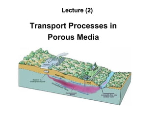
  • 2. Lecture (2)Lecture (2) 1. After how many years the contaminant reaches a river or a water supply well? 2. What is the level of concentration at the well?
  • 3. Layout of the LectureLayout of the Lecture • Transport Processes in Porous Media.Transport Processes in Porous Media. • Derivation of The Transport Equation (ADE).Derivation of The Transport Equation (ADE). • Methods of Solution.Methods of Solution. • Effect of Heterogeneity on Transport:Effect of Heterogeneity on Transport: Laboratory Experiments (movie).Laboratory Experiments (movie).
  • 4. Transport ProcessesTransport Processes 1)1) Physical :Physical : Advection-Diffusion-DispersionAdvection-Diffusion-Dispersion 2) Chemical:2) Chemical: Adsorption- Ion Exchange- etc.Adsorption- Ion Exchange- etc. 3) Biological:3) Biological: Micro-organisms ActivityMicro-organisms Activity (Bacteria&Microbes)(Bacteria&Microbes) 4) Decay:4) Decay: Radioactive Decay-Natural Attenuation.Radioactive Decay-Natural Attenuation.
  • 5. Physical ProcessesPhysical Processes 1. Advection 2. Molecular Diffusion 3. Mechanical Dispersion 4. Hydrodynamic Dispersion
  • 6. Advection (Convection)Advection (Convection) adv J Cq= Advective Solute Mass Flux: .q = K− ∇Φ is the advective solute mass flux, is the solute concentration, and is the water flux (specific discharge) given by Darcy's law: C q adv J
  • 7. Molecular DiffusionMolecular Diffusion Diffusive Flux in Bulk: (Fick’s Law of Diffusion) is the diffusive solute mass flux in bulk, dif o oJ = - D C∇ dif oJ is the solute concentration gradient,C∇ is the molecular diffusive coefficient in bulk.oD Random Particle motion Time t1 t2 t3 t4
  • 8. Molecular Diffusion (Cont.)Molecular Diffusion (Cont.) dif effJ = - D C∇ τ O eff D D = Diffusive Flux in Porous Medium is the effective molecular diffusion coefficient in porous medium, effD τ is a tortuosity factor ( = 1.4) 0.7eff oD D:
  • 9. Mechanical DispersionMechanical Dispersion dis J = - Cε ∇.D Depressive Flux in Porous Media (Fick’s Law): is the depressive solute mass flux, is the solute concentration gradient, is the dispersion tensor, is the effective porosity dis J ε C∇ D xx xy xz yx yy yz zx zy zz D D D D D D D D D     =       D [after Kinzelbach, 1986] Causes of Mechanical Dispersion
  • 10. Hydrodynamic DispersionHydrodynamic Dispersion ( ) ( ) i j ij efft ij l t v v = |v|+ + -D D |v| α δ α α _hydo dis J = - Cε ∇.D Hydrodynamic Depressive Flux in Porous Media (Fick’s Law): The components of the dispersion tensor in isotropic soil is given by [Bear, 1972], is Kronecker delta, =1 for i=j and =0 for i≠ j,ijδ are velocity components in two perpendicular directions,i jv v is the magnitude of the resultant velocity,v 2 2 2 i j kv v v v= + + is the longitudinal pore-(micro-) scale dispersivity, andlα tα is the transverse pore-(micro-) scale dispersivity ijδ ijδ
  • 11. Hydrodynamic Dispersion (Cont.)Hydrodynamic Dispersion (Cont.) In case of flow coincides with the horizontal x-direction all off-diagonal terms are zeros and one gets, 0 0 0 0 0 0 xx yy zz D D D    =      D xx effl yy efft zz efft = |v|+D D = |v|+D D = |v|+D D α α α , 0.5 , 0.0157 3.5 Random packing is the grain diameter l l p l t t p t p c d c c d c d α σ α σ σ = = = = =
  • 12. Dispersion Regimes at Micro-ScaleDispersion Regimes at Micro-Scale D VL Pe eff cc = Peclet Number: Advection/Dispersion Perkins and Johnston, 1963
  • 13. Chemical ProcessesChemical Processes • Sorption & De-sorption.Sorption & De-sorption. • Ion Exchange.Ion Exchange. • Retardation.Retardation.
  • 14. Adsorption IsothermsAdsorption Isotherms )(CfS = m bCS = CKS d= 21 kCkS += 4 3 1 k Ck S + = Freundlich (1926) Langmuir (1915, 1918)
  • 15. Biological ProcessesBiological Processes •Biological Degradation and Natural Attenuation. •Micro-organisms Activity. •Decay. C dt Cd λε−= ε )( is the decay coefficient
  • 16. Transport Through Porous MediaTransport Through Porous Media
  • 17. Derivation of Transport Equation inDerivation of Transport Equation in Rectangular CoordinatesRectangular Coordinates Flow In – Flow Out = rate of change within the control volume
  • 18. Solute Flux in the x-directionSolute Flux in the x-direction ( ) ( ) ( ) in adv dis x x x adv dis out adv dis x x x x x J J J y z J J J J J x y z x ∂ ∂ = + ∆ ∆  + = + + ∆ ∆ ∆   
  • 19. Solute Flux in the y-directionSolute Flux in the y-direction ( ) ( ) ( ) in adv dis y y y adv dis y yout adv dis y y y J J J x z J J J J J y x z y ∂ ∂ = + ∆ ∆  + = + + ∆ ∆ ∆    
  • 20. Solute Flux in the z-directionSolute Flux in the z-direction ( ) ( ) ( ) in adv dis z z z adv dis out adv dis z z z z z J J J y x J J J J J z y x z ∂ ∂ = + ∆ ∆  + = + + ∆ ∆ ∆   
  • 21. From Continuity of Solute MassFrom Continuity of Solute Mass ( )solute in out M J J C x y z t t ∂ ∂ ε ∂ ∂ − = = ∆ ∆ ∆∑ ∑ Where ε is the porosity, and C is Concentration of the solute.
  • 22. From Continuity of Solute MassFrom Continuity of Solute Mass ( ) ( ) ( ) ( ) ( ) ( ) ( ) ( ) ( ) ( ) adv dis adv dis adv dis x x y y z z adv dis adv dis x x x x adv dis y yadv dis y y adv dis adv dis z z z z J J y z J J x z J J y x J J J J x y z x J J J J y x z y J J J J z y x z C x y z t ∂ ∂ ∂ ∂ ∂ ∂ ∂ ε ∂ + ∆ ∆ + + ∆ ∆ + + ∆ ∆  + − + + ∆ ∆ ∆     + − + + ∆ ∆ ∆      + − + + ∆ ∆ ∆    = ∆ ∆ ∆
  • 23. By canceling out termsBy canceling out terms ( )( ) ( ) adv disadv dis adv dis y yx x z z J JJ J J J z y x x y z ∂∂ ∂ ∂ ∂ ∂  ++ + − + + ∆ ∆ ∆     (C x y z t ∂ ε ∂ = ∆ ∆ ∆ ) ( )( ) ( ) ( ) adv disadv dis adv dis y yx x z z J JJ J J J x y z C t ∂∂ ∂ ∂ ∂ ∂ ∂ ε ∂  ++ + − + +     =
  • 24. Assuming Advection and HydrodynamicAssuming Advection and Hydrodynamic DispersionDispersion , , , adv dis x x x xx xx adv dis y y y yy yy adv dis z z z zz zz C J = Cq J = - D C - D x C J = Cq J = - D C - D y C J = Cq J = - D C - D z ε ε ε ε ε ε ∂ ∇ = ∂ ∂ ∇ = ∂ ∂ ∇ = ∂ . . . . . .
  • 25. Solute Transport Through Porous Media bySolute Transport Through Porous Media by advection and dispersion processesadvection and dispersion processes ( ) y yyx xx z zz CC C Cq - DCq - D Cq - D yx z x y z C t ∂ ε∂ ε ∂ ε ∂ ∂ ∂ ∂ ε ∂   ∂∂ ∂      ÷ ÷  ÷∂∂ ∂      − + +       = .. . ( ) ( ) ( ) Hyperbolic Part x y z Parabolic Part xx yy zz C v C v C v C t x y z C C C D D D x x y y z z ∂ ∂ ∂ ∂ ∂ ∂ ∂ ∂ ∂ ∂ ∂ ∂ ∂ ∂ ∂ ∂ ∂ ∂ ∂ ∂ = − − −      + + + ÷ ÷  ÷      644444474444448 644444444474444444448
  • 26. General Form of The Transport EquationGeneral Form of The Transport Equation   [ ] } } / ( ') Dispersion Diffusion Advection Source SinkChemical reaction Decay ij i i j i C C S C C W v C + Q CD t x x x λ ε ε − −  ∂ ∂ ∂ ∂ − = − − +  ∂ ∂ ∂ ∂   6447448 64748 64748 where C is the concentration field at time t, Dij is the hydrodynamic dispersion tensor, Q is the volumetric flow rate per unit volume of the source or sink, S is solute concentration of species in the source or sink fluid, i, j are counters, C’ is the concentration of the dissolved solutes in a source or sink, W is a general term for source or sink and vi is the component of the Eulerian interstitial velocity in xi direction defined as follows,              ij i j K = -v xε ∂Φ ∂ where Kij is the hydraulic conductivity tensor, and ε is the porosity of the medium.
  • 27. Schematic Description of ProcessesSchematic Description of Processes Figure 7. Schematic Description of the Effects of Advection, Dispersion, Adsorption, and Degradation on Pollution Transport [after Kinzelbach, 1986]. Advection+Dispersion Advection Advection+Dispersion+Adsorption Advection+Dispersion+Adsorption+Degradation
  • 28. Methods of SolutionMethods of Solution 1) Analytical Approaches:1) Analytical Approaches: 2) Numerical Approaches:2) Numerical Approaches: i)i) Eulerian Methods:(FDM,FEM).Eulerian Methods:(FDM,FEM). ii) Lagrangian Methods:(RWM).ii) Lagrangian Methods:(RWM). iii) Eulerian-Lagrangian Methods:iii) Eulerian-Lagrangian Methods: (MOC).(MOC).
  • 29. Pulse versus Continuous InjectionPulse versus Continuous Injection Concentration Distribution in case of Pulse and Continuous Injections in a 2D Field [after Kinzelbach, 1986].       tV4 )Y-(y + tV4 )tV-X-(x - tV4tV4 H)/(M =t)y,C(x, xt 2 o xl 2 xo xtxl o αααπαπ ε exp ( ) d tV4 Y-y + tV4 tV-X-x - tV4 HM=ty,x,C t xt 2 o xl 2 xo tlx o ∫       −− − − • 0 )( )( )( )(( exp 1)(/ )( τ τατα τ τααπ ε
  • 30. Flow t = 0 f t = Flowing Time Var(X) The spread of the front is a measure of the heterogeneity Random WalkRandom Walk
  • 31. Analytical versus Random WalkAnalytical versus Random Walk
  • 32. Scale dependent dispersivityScale dependent dispersivity