Top Rated Pune Call Girls Budhwar Peth ⟟ 6297143586 ⟟ Call Me For Genuine Se...
05 navigation
1. 5
Chapter
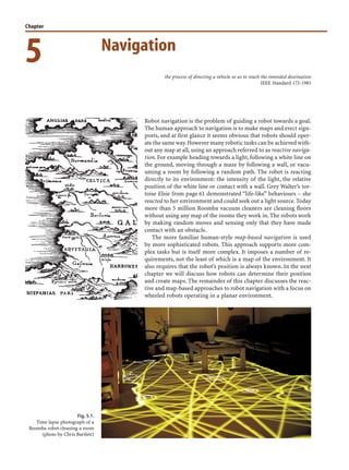
Robot navigation is the problem of guiding a robot towards a goal.
The human approach to navigation is to make maps and erect sign-
posts, and at first glance it seems obvious that robots should oper-
ate the same way.However many robotic tasks can be achieved with-
out any map at all,using an approach referred to as reactive naviga-
tion. For example heading towards a light, following a white line on
the ground, moving through a maze by following a wall, or vacu-
uming a room by following a random path. The robot is reacting
directly to its environment: the intensity of the light, the relative
position of the white line or contact with a wall. Grey Walter’s tor-
toise Elsie from page 61 demonstrated “life-like” behaviours – she
reacted to her environment and could seek out a light source. Today
more than 5 million Roomba vacuum cleaners are cleaning floors
without using any map of the rooms they work in. The robots work
by making random moves and sensing only that they have made
contact with an obstacle.
The more familiar human-style map-based navigation is used
by more sophisticated robots. This approach supports more com-
plex tasks but is itself more complex. It imposes a number of re-
quirements, not the least of which is a map of the environment. It
also requires that the robot’s position is always known. In the next
chapter we will discuss how robots can determine their position
and create maps. The remainder of this chapter discusses the reac-
tive and map-based approaches to robot navigation with a focus on
wheeled robots operating in a planar environment.
Navigation
the process of directing a vehicle so as to reach the intended destination
IEEE Standard 172-1983
Fig. 5.1.
Time lapse photograph of a
Roomba robot cleaning a room
(photo by Chris Bartlett)
3. 89
To ascend the gradient we need to estimate the gradient direction at the current
location and this requires at least two measurements of the field. In this example we
use two sensors, bilateral sensing, with one on each side of the robot’s body. The sen-
sors are modelled by the green sensor blocks shown in Fig. 5.2 and are parameterized
by the position of the sensor with respect to the robot’s body,and the sensing function.
In this example the sensors are at ±2 units in the vehicle’s lateral or y-direction.
The field to be sensed is a simple inverse square field defined by
1 function sensor = sensorfield(x, y)
2 xc = 60; yc = 90;
3 sensor = 200./((x-xc).^2 + (y-yc).^2 + 200);
which returns the sensor value s(x, y) ∈ [0, 1] which is a function of the sensor’s posi-
tion in the plane. This particular function has a peak value at the point (60, 90).
The vehicle speed is
where sR and sL are the right and left sensor readings respectively. At the goal, where
sR = sL = 1 the velocity becomes zero.
Steering angle is based on the difference between the sensor readings
sowhenthefieldisequalintheleft-andright-handsensorstherobotmovesstraightahead.
We start the simulation from the Simulink® menu or the command line
>> sim('sl_braitenberg');
and the path of the robot is shown in Fig. 5.3.The starting pose can be changed through
the parameters of the Bicycle block.We see that the robot turns toward the goal and
slows down as it approaches, asymptotically achieving the goal position.
This particular sensor-action control law results in a specific robotic behaviour.We
could add additional logic to the robot to detect that it had arrived near the goal and
then switch to a stopping behaviour.An obstacle would block this robot since its only
behaviour is to steer toward the goal, but an additional behaviour could be added to
handle this case and drive around an obstacle. We could add another behaviour to
search randomly for the source if none was visible. Grey Walter’s tortoise had four
behaviours and switching was based on light level and a touch sensor.
Fig. 5.2. The Simulink® model
sl_braitenberg drives the
vehicle toward the maxima of a
provided scalar function. The ve-
hicle plus controller is an example
of a Braitenberg vehicle
Wecanmakethemeasurementssimul-
taneouslyusingtwospatiallyseparated
sensors or from one sensor over time as
the robot moves.
Similar strategies are used by moths
whose two antennae are exquisitely
sensitive odor detectors that are used
to steer a male moth toward a phero-
mone emitting female.
5.1 · Reactive Navigation
4. 90
Multiple behaviours and the ability to switch between them leads to an approach
known as behaviour-based robotics. The subsumption architecture was proposed as a
means to formalize the interaction between different behaviours.Complex,some might
say intelligent looking,behaviours can be manifested by such systems.However as more
behaviours are added the complexity of the system grows rapidly and interactions
between behaviours become more complex to express and debug. Ultimately the pen-
alty of not using a map becomes too great.
5.1.2 lSimple Automata
Another class of reactive robots are known as bugs – simple automata that perform
goal seeking in the presence of non-driveable areas or obstacles. There are a large
number of bug algorithms and they share the ability to sense when they are in proxim-
ity to an obstacle. In this respect they are similar to the Braitenberg class vehicle, but
the bug includes a state machine and other logic in between the sensor and the motors.
The automata have memory which our earlier Braitenberg vehicle lacked. In this
section we will investigate a specific bug algorithm known as bug2.
We start by loading an obstacle field to challenge the robot
>> load map1
which defines a 100 × 100 matrix variable map in the workspace. The elements are
zero or one representing free space orobstacle respectively and this is shown in Fig. 5.4.
Tools to generate such maps are discussed on page 92. This matrix is an example of an
occupancy grid which will be discussed further in the next section.
At this point we state some assumptions. Firstly, the robot operates in a grid world
and occupies one grid cell. Secondly, the robot does not have any non-holonomic con-
straints and can move to any neighbouring grid cell. Thirdly, it is able to determine its
position on the plane which is a non-trivial problem that will be discussed in detail in
Chap. 6. Finally, the robot can only sense its immediate locale and the goal. The robot
does not use the map – the map is used by the simulator to provide sensory inputs to
the robot.
We create an instance of the bug2 class
>> bug = Bug2(map);
and the goal is
>> bug.goal = [50; 35];
Fig. 5.3.
Path of the Braitenberg vehicle
moving toward (and past) the
maximum of a 2D scalar field
whose magnitude is shown
color coded
Braitenberg’s book describes a series of
increasingly complex vehicles, some of
which incorporate memory. However
the term Braitenberg vehicle has be-
come associated with the simplest ve-
hicles he described.
Chapter 5 · Navigation
5. 91
The simulation is run using the path method
>> bug.path([20; 10]);
where the argument is the initial position of the robot.The method displays an anima-
tion of the robot moving toward the goal and the path is shown as a series of green
dots in Fig. 5.4.
The strategy of the bug2 algorithm is quite simple. It moves along a straight line
towards its goal. If it encounters an obstacle it moves around the obstacle (always
counter-clockwise) until it encounters a point that lies along its original line that is
closer to the goal than where it first encountered the obstacle.
If an output argument is specified
>> p = bug.path([20; 10]);
it returns the path as a matrix p
>> about(p)
p [double] : 332x2 (5312 bytes)
which has one row per point, and comprises 332 points for this example. Invoking the
function without the starting position
>> p = bug.path();
will prompt for a starting point to be selected by clicking on the plot.
The bug2 algorithms has taken a path that is clearly not optimal. It has wasted time
by continuing to follow the perimeter of the obstacle until it rejoined its original line.
It would also have been quicker in this case to go clockwise around the obstacle.Many
variants of the bug algorithm have been developed, but while they improve the perfor-
mance for one type of environment they can degrade performance in others. Funda-
mentally the robot is limited by not using a map. It cannot see the big picture and
therefore takes paths that are locally, rather than globally, optimal.
5.2 lMap-Based Planning
The key to achieving the best path between points A and B, as we know from every-
day life, is to use a map. Typically best means the shortest distance but it may also
include some penalty term or cost related to traversability which is how easy the ter-
rain is to drive over – it might be quicker to travel further but over better roads. A
more sophisticated planner might also consider the kinematics and dynamics of the
Fig. 5.4.
The path taken by the bug2
algorithm is marked by green
dots. The goal is a blue diamond,
the black dashed line is the M-
line, the direct path from the
start to the goal. Obstacles are
indicated by red pixels
It could be argued that the M-line rep-
resents an explicit plan.Thus bug algo-
rithms occupy a position somewhere
between Braitenberg vehicles and
map-based planning systems in the
spectrum of approaches to navigation.
Beyond the trivial straight line case.
5.2 · Map-Based Planning
6. 92
vehicle and avoid paths that involve turns that are tighter than the vehicle can execute.
Recalling our earlier definition of a robot as a
goal oriented machine that can sense, plan and act,
this section concentrates on planning.
There are many ways to represent a map and the position of the vehicle within the
map. One approach is to represent the vehicle position as (x, y) ∈ R2
and the the
driveable regions or obstacles as polygons, each comprising lists of vertices or edges.
This is potentially a very compact format but determining potential collisions between
the robot and obstacles may involve testing against long lists of edges.
A simpler and very computer-friendly representation is the occupancy grid.As its
name implies the world is treated as a grid of cells and each cell is marked as occu-
pied or unoccupied. We use zero to indicate an unoccupied cell or free space where
the robot can drive. A value of one indicates an occupied or non-driveable cell. The
size of the cell depends on the application. The memory required to hold the occu-
pancy grid increases with the spatial area represented and inversely with the cell size.
However for modern computers this representation is very feasible. For example a
cell size 1 × 1 m requires just 125 kbyte km–2.
In the remainder of this section we use code examples to illustrate several differ-
ent planners and all are based on the occupancy grid representation. To create uni-
formity the planners are all implemented as classes derived from the Navigation
superclass which is briefly described on page 93. The bug2 class we used previously
was also an instance of this class so the remaining examples follow a familiar pattern.
Once again we state some assumptions. Firstly, the robot operates in a grid world
and occupies one grid cell. Secondly, the robot does not have any non-holonomic
constraints and can move to any neighbouring grid cell. Thirdly, it is able to deter-
mine its position on the plane. Fourthly, the robot is able to use the map to compute
the path it will take.
Making a map. An occupancy grid is a matrix that corresponds to a region of 2-dimensional
space. Elements containing zeros are free space where the robot can move, and those with ones
are obstacles where the robot cannot move. We can use many approaches to create a map. For
example we could create a matrix filled with zeros (representing all free space)
>> map = zeros(100, 100);
and use MATLAB® operations such as
>> map(40:50,20:80) = 1;
to create an obstacle but this is quite cumbersome. Instead we can use the Toolbox map editor
makemap to create more complex maps using a simple interactive editor
>> map = makemap(100)
makeworld:
left button, click and drag to create a rectangle
p - draw polygon
c - draw circle
e - erase map
u - undo last action
q - leave editing mode
which allows you to add rectangles, circles and polygons to an occupancy grid, in this example
the grid is 100 × 100.
Note that the occupancy grid is a matrix whose coordinates are conventionally expressed as
(row,column) and the row is the vertical dimension of a matrix.We use the Cartesian convention
of a horizontal x-coordinate first, followed by the y-coordinate therefore the matrix is always
indexed as y,x in the code.
Considering a single bit to represent
each cell.The occupancy grid could be
compressed or could be kept on a disk
with only the local region in memory.
Chapter 5 · Navigation
7. 93
In all examples we use the following parameters
>> goal = [50; 30];
>> start = [20; 10];
>> load map1
for the goal position, start position and world map respectively. The world map is
loaded into the workspace variable map. These parameters can be varied, and the oc-
cupancy grid changed using the tools described on page 92.
5.2.1 lDistance Transform
Consider a matrix of zeros with just a single non-zero element representing the goal.
The distance transform of this matrix is another matrix, of the same size, but the
value of each element is its distance from the original non-zero pixel.For robot path
planning we use the default Euclidean distance. The distance transform is actually an
image processing technique and will be discussed further in Chap. 12.
Fig. 5.5.
The distance transform path.
Obstacles are indicated by red
cells. The background grey
intensity represents the cell’s
distance from the goal in units
of cell size as indicated by the
scale on the right-hand side
Navigation superclass. The examples in this chapter are all based on classes derived from the
Navigationclass which is designed for 2D grid-based navigation.Each example consists of essen-
tially the following pattern.Firstly we create an instance of an object derived from the Navigation
class by calling the class constructor.
>> nav = MyNavClass(world)
which is passed the occupancy grid. Then a plan to reach the goal is computed
>> nav.plan(goal)
The plan can be visualized by
>> nav.visualize()
and a path from an initial position to the goal is computed by
>> p = nav.path(start)
>> p = nav.path()
where p is the path, a sequence of points from start to goal, one row per point, and each row
comprises the x- and y-coordinate.If start is not specified,as in the second example,the user is
prompted to interactively click the start point.If no output argument is provided an animation of
the robot’s motion is displayed.
The distance between two points
(x1, y1)and(x2, y2)where∆x = x2 − x1
and ∆y = y2 − y1 can be Euclidean
_∆x
2
g+g∆gy
2
orCityBlock(alsoknownas
Manhattan) distance |∆x| + |∆y|.
5.2 · Map-Based Planning
8. 94
To use the distance transform for robot navigation we create a DXform object,
which is derived from the Navigation class
>> dx = DXform(map);
and create a plan to reach the specified goal
>> dx.plan(goal)
which can be visualized
>> dx.visualize()
as shown in Fig. 5.5.We see the obstacle regions in red and the background grey level at
any point indicates the distance from that point to the goal, taking into account travel
around the obstacle.
The hard work has been done and finding a path from any point to the goal is now very
simple.Wherevertherobotstarts,itmovestotheneighbouringcellthathasthesmallestdis-
tancetothegoal.Theprocessisrepeateduntiltherobotreachesacellwithadistancevalueof
zero which is the goal.For example to find a path from to the goal from position start is
>> dx.path(start);
which displays an animation of the robot moving toward the goal. The path is indi-
cated by a series of green dots as shown in Fig. 5.5.
If the path method is called with an output argument the animation is skipped
and the path
>> p = dx.path(start);
is returned as a matrix, one row per point, which we can visualize
>> dx.visualize(p)
The path comprises
>> numrows(p)
ans =
205
points which is shorter than the path found by bug2. Unlike bug2 this planner has
found the shorter clockwise path around the obstacle.
This navigation algorithm has exploited its global view of the world and has,through
exhaustive computation, found the shortest possible path. In contrast, bug2 without
the global view has just bumped its way through the world. The penalty for achieving
the optimal path is computational cost. The distance transform is iterative. Each itera-
tion has a cost of O(N2
) and the number of iterations is at least O(N), where N is the
dimension of the map.
We can visualize the iterations of the distance transform by
>> dx.plan(goal, show 0.1);
which shows the distance values propagating as a wavefront outward from the goal.
The wavefront moves upward, splits to the left and right, moves downward and the
two fronts collide at the bottom of the map along the line x = 32. The last argument
specifies a pause of 0.1 s between frames. Although the plan is expensive to create,
once it has been created it can be used to plan a path from any initial point to the goal.
We have converted a fairly complex planning problem into one that can now be
handled by a Braitenberg-class robot that makes local decisions based on the distance
to the goal. Effectively the robot is rolling downhill on the distance function which we
can plot as a 3D surface
>> dx.visualize3d(p)
shown in Fig. 5.6 with the robot’s path overlaid.
Chapter 5 · Navigation
9. 95
For large occupancy grids this approach to planning will become impractical. The
roadmap methods that we discuss later in this chapter provide an effective means to
find paths in large maps at greatly reduced computational cost.
5.2.2 lD*
A popular algorithm for robot path planning is called D*
, and it has a number of fea-
tures that are useful for real-world applications. D*
generalizes the occupancy grid to
a cost map which represents the cost c ∈ R, c > 0 of traversing each cell in the hori-
zontal or vertical direction. The cost of traversing the cell diagonally is c2. For cells
corresponding to obstacles c = ∞ (Inf in MATLAB®).
D*
finds the path which minimizes the total cost of travel.If we are interested in the
shortest time to reach the goal then cost is the time to drive across the cell and is
inversely related to traversability. If we are interested in minimizing damage to the
vehicle or maximizing passenger comfort then cost might be related to the roughness
of the terrain within the cell. The costs assigned to cells will depend on the character-
istics of the vehicle: a large 4-wheel drive vehicle may have a finite cost to cross a rough
area whereas for a small car that cost might be infinite.
The key feature of D*
is that it supports incremental replanning. This is important
if, while we are moving, we discover that the world is different to our map. If we dis-
cover that a route has a higher than expected cost or is completely blocked we can
incrementally replan to find a better path. The incremental replanning has a lower
computational cost than completely replanning as would be required using the dis-
tance transform method just discussed.
To implement the D*
planner using the Toolbox we use a similar pattern and first
create a D*
navigation object
>> ds = Dstar(map);
The D*
planner converts the passed occupancy grid map into a cost map which we can
retrieve
>> c = ds.costmap();
where the elements of c will be 1 or ∞ representing free and occupied cells respectively.
Fig. 5.6.
The distance transform as a
3D function, where height is
distance from the goal.Navigation
is simply a downhill run. Note
the discontinuity in the distance
transform where the split wave-
fronts met
D*
is an extension of the A*
algorithm
for finding minimum cost paths through
a graph, see Appendix J.
5.2 · Map-Based Planning
10. 96
A plan for moving to the goal is generated by
>> ds.plan(goal);
which creates a very dense directed graph (see Appendix J). Every cell is a graph vertex
and has a cost,a distance to the goal,and a link to the neighbouring cell that is closest to
the goal.Each cell also has a state t ∈ {NEW, OPEN, CLOSED}.Initially every cell is in the
NEW state,the cost of the goal cell is zero and its state is OPEN.We can consider the set of
all cells in the OPEN state as a wavefront propagating outward from the goal. The cost of
reaching cells that are neighbours of an OPEN cell is computed and these cells in turn are
set to OPEN and the original cell is removed from the open list and becomes CLOSED.In
MATLAB® this initial planning phase is quite slow and takes tens of seconds and
>> ds.niter
ans =
10558
iterations of the planning loop.
The path from an arbitrary starting point to the goal
>> ds.path(start);
is shown in Fig. 5.7.The robot has again taken the short path to the left of the obstacles
and is almost the same as that generated by the distance transform.
The real power of D*
comes from being able to efficiently change the cost map dur-
ing the mission. This is actually quite a common requirement in robotics since real
sensors have a finite range and a robot discovers more of world as it proceeds. We
inform D*
about changes using the modify_cost method, for example
>> for y=78:85
>> for x=12:45
>> ds.modify_cost([x,y], 2);
>> end
>> end
where we have raised the cost to 2 for a small rectangular region to simulate a patch of
terrain with lower traversability. This region is indicated by the white dashed rect-
angle in Fig. 5.8. The other driveable cells have a cost of 1. The plan is updated by
invoking the planning algorithm again
>> ds.plan();
but this time the number of iterations is only
>> ds.niter
ans =
3178
Fig. 5.7.
The D*
planner path. Obstacles
are indicated by red cells and all
driveable cells have a cost of 1.
The background grey intensity
represents the cell’s distance from
the goal in units of cell size as
indicated by the scale on the
right-hand side
The distance transform also evolves as
a wavefront outward from the goal.
HoweverD*
representsthefrontiereffi-
ciently as a list of cells whereas the dis-
tance transform computes the frontier
on a per-pixel basis at every iteration –
thefrontierisimplicitlywhereacellwith
infinitecost(theinitialvalueofallcells)
is adjacent to a cell with finite cost.
D*
is more efficient than the distance
transform but it executes more slowly
because it is implemented entirely in
MATLAB® code whereas the distance
transform is a MEX-file written in C.
Chapter 5 · Navigation
11. 97
which is 30% of that required to create the original plan. The new path for the robot
>> ds.path(start);
is shown in Fig. 5.8.The cost change is relatively small but we notice that the increased
cost of driving within this region is indicated by a subtle brightening of those cells – in
a cost sense these cells are now further from the goal. Compared to Fig. 5.7 the robot’s
path has moved to the right in order to minimize the distance it travels through the
high-cost region. D*
allows updates to the map to be made at any time while the robot
is moving.After replanning the robot simply moves to the adjacent cell with the lowest
cost which ensures continuity of motion even if the plan has changed.
5.2.3 lVoronoi Roadmap Method
In planning terminology the creation of a plan is referred to as the planning phase.
The query phase uses the result of the planning phase to find a path from A to B. The
two previous planning algorithms, distance transform and D*
, require a significant
amount of computation for the planning phase, but the query phase is very cheap.
However the plan depends on the goal. If the goal changes the expensive planning
phase must be re-executed. Even though D*
allows the path to be recomputed as the
costmap changes it does not support a changing goal.
The disparity in planning and query costs has led to the development of roadmap
methods where the query can include both the start and goal positions. The planning
phase provides analysis that supports changing starting points and changing goals. A
good analogy is making a journey by train. We first find a local path to the nearest
train station, travel through the train network, get off at the station closest to our goal,
and then take a local path to the goal. The train network is invariant and planning a
path through the train network is straightforward. Planning paths to and from the
entry and exit stations respectively is also straightforward since they are, ideally, short
Fig. 5.8.
Path from D*
planner with modi-
fied map. The higher-cost region
is indicated by the white dashed
rectangle and has changed the
path compared to Fig. 5.7
A graphis an abstract representation of a set of objects connected by links typically denoted G(V, E)
and depicted diagrammatically as shown to the left.The objects, V,are called vertices or nodes,and
the links, E, that connect some pairs of vertices are called edges or arcs. Edges can be directed (ar-
rows) or undirected as in this case. Edges can have an associated weight or cost associated with
moving from one of its vertices to the other. A sequence of edges from one vertex to another is a
path.Graphs can be used to represent transport or communications networks and even social rela-
tionships, and the branch of mathematics is graph theory. Minimum cost path between two nodes
in the graph can be computed using well known algorithms such as Dijstrka’s method or A*
.
The navigation classes use a simple MATLAB® graph class called PGraph, see Appendix J.
5.2 · Map-Based Planning
12. 98
paths. The robot navigation problem then becomes one of building a network of ob-
stacle free paths through the environment which serve the function of the train net-
work. In the literature such a network is referred to as a roadmap. The roadmap need
only be computed once and can then be used like the train network to get us from any
start location to any goal location.
We will illustrate the principles by creating a roadmap from the occupancy grid’s
free space using some image processing techniques.The essential steps in creating the
roadmap are shown in Fig. 5.9. The first step is to find the free space in the map which
is simply the complement of the occupied space
>> free = 1 - map;
and is a matrix with non-zero elements where the robot is free to move.The boundary
is also an obstacle so we mark the outermost cells as being not free
>> free(1,:) = 0; free(100,:) = 0;
>> free(:,1) = 0; free(:,100) = 0;
and this map is shown in Fig. 5.9a where free space is depicted as white.
The topological skeleton of the free space is computed by a morphological image
processing algorithm known as thinning applied to the free space of Fig. 5.9a
>> skeleton = ithin(free);
and the result is shown in Fig. 5.9b.We see that the obstacles have grown and the free
space, the white cells, have become a thin network of connected white cells which are
Fig. 5.9. Steps in the creation of a
Voronoi roadmap. a Free space is
indicatedbywhitecells,b theskel-
eton of the free space is a network
of adjacent cells no more than one
cell thick, c the skeleton with the
obstaclesoverlaidinredandroad-
map junction points indicated in
blue. d the distance transform of
the obstacles, pixel values corre-
spond to distance to the nearest
obstacle
Chapter 5 · Navigation
13. 99
equidistant from the boundaries of the original obstacles.Image processing functions,
and morphological operations in particular, will be explained more fully in Chap. 12.
Figure 5.9c shows the free space network overlaid on the original map. We have
created a network of paths that span the space and which can be used for obstacle-free
travel around the map. These paths are the edges of a generalized Voronoi diagram.
We could obtain a similar result by computing the distance transform of the obstacles,
Fig. 5.9a, and this is shown in Fig. 5.9d. The value of each pixel is the distance to the
nearest obstacle and the ridge lines correspond to the skeleton of Fig. 5.9b. Thinning
or skeletonization, like the distance transform, is a computationally expensive itera-
tive algorithm but it illustrates well the principles of finding paths through free space.
In the next section we will examine a cheaper alternative.
5.2.4 lProbabilistic Roadmap Method
The high computational cost of the distance transform and skeletonization methods
makes them infeasible for large maps and has led to the development of probabilistic
methods. These methods sparsely sample the world map and the most well known of
these methods is the probabilistic roadmap or PRM method.
To use the Toolbox PRM planner for our problem we first create a PRM object
>> prm = PRM(map)
and then create the plan
>> prm.plan()
Note that in this case we do not pass goal as an argument to the planner since the
plan is independent of the goal. Creating the path is a two phase process: planning,
and query. The planning phase finds N random points, 100 by default, that lie in free
space. Each point is connected to its nearest neighbours by a straight line path that
does not cross any obstacles, so as to create a network, or graph, with a minimal num-
ber of disjoint components and no cycles. The advantage of PRM is that relatively few
points need to be tested to ascertain that the points and the paths between them are
obstacle free. The resulting network is stored within the PRM object and a summary
can be displayed
>> prm
prm =
PRM: 100x100
graph size: 100
dist thresh: 30.000000
100 vertices
712 edges
3 components
TheVoronoi tessellation of a set of planar points,known as sites,is a set of Voronoi cells as shown
to the left.Each cell corresponds to a site and consists of all points that are closer to its site than to
any other site. The edges of the cells are the points that are equidistant to the two nearest sites.A
generalized Voronoi diagram comprises cells defined by measuring distances to objects rather
than points. In MATLAB® we can generate a Voronoi diagram by
>> sites = rand(10,2)
>> voronoi(sites(:,1), sites(:,2))
Georgy Voronoi (1868–1908) was a Russian mathematician, born in what is now Ukraine. He
studied at Saint Petersburg University and was a student of Andrey Markov. One of his students
Boris Delaunay defined the eponymous triangulation which has dual properties with theVoronoi
diagram.
The junctions in the roadmap are indi-
cated by blue circles. The junctions, or
triple points, are identified using the
morphological image processing func-
tion triplepoint.
5.2 · Map-Based Planning
To replicate the following result be sure
toinitializetherandomnumbergenera-
tor first using randinit. See p. 101.
14. 100
which indicates the number of edges and connected components in the graph. The
graph can be visualized
>> prm.visualize()
as shown in Fig. 5.10a. The dots represent the randomly selected points and the lines
are obstacle-free paths between the points. Only paths less than 30 cells long are se-
lected which is the distance threshold parameter of the PRM class. Each edge of the
graph has an associated cost which is the distance between its two nodes. The color of
the node indicates which component it belongs to and each component is assigned a
unique color. We see two nodes on the left-hand side that are disconnected from the
bulk of the roadmap.
The query phase is to find a path from the start point to the goal. This is simply a
matter of moving to the closest node in the roadmap, following the roadmap, and
getting off at the node closest to the goal and
>> prm.path(start, goal)
shows an animation of the robot moving through the graph and the path followed is
shown in Fig. 5.11.Note that this time we provide the start and the goal position to the
query phase. The next node on the roadmap is indicated in yellow and a line of green
dots shows the robot’s path. Travel along the roadmap involves moving toward the
neighbouring node which has the lowest cost, that is, closest to the goal.We repeat the
process until we arrive at the node in the graph closest to the goal, and from there we
move directly to the goal.
An advantage of this planner is that once the roadmap is created by the planning
phase we can change the goal and starting points very cheaply, only the query phase
needs to be repeated.
However the path is not optimal and the distance travelled
>> p = prm.path(start, goal);
>> numcols(p)
ans =
299
is greater than the optimal value found by the distance transform but less than that
found by bug2.
There are some important tradeoffs in achieving this computational efficiency.
Firstly,the underlying random sampling of the free space means that a different graph
is created every time the planner is run, resulting in different paths and path lengths.
For example rerunning the planner
>> prm.plan();
Fig. 5.10. Probablistic roadmap
(PRM) planner and the random
graphs produced in the planning
phase. a Almost fully connected
graph, apart from two nodes on
the left-hand edge, b graph with
a large disconnected component
Chapter 5 · Navigation
15. 101
Fig. 5.11.
Probablistic roadmap (PRM)
planner showing the path taken
by the robot, shown as green
dots. The nodes of the roadmap
that are visited are highlighted
in yellow
Random numbers. The MATLAB® random number generator (used for rand and randn) gen-
erates a very long sequence of numbers that are an excellent approximation to a random se-
quence. The generator maintains an internal state which is effectively the position within the
sequence. After startup MATLAB® always generates the following random number sequence
>> rand
ans =
0.8147
>> rand
ans =
0.9058
>> rand
ans =
0.1270
Many algorithms discussed in this book make use of random numbers and this means that the
resultscanneverberepeated.Before all suchexamples inthisbookisaninvisiblecall torandinit
which resets the random number generator to a known state
>> randinit
>> rand
ans =
0.8147
>> rand
ans =
0.9058
and we see that the random sequence has been restarted.
A real robot is not a point. We have assumed that the robot is a point, occupying a single cell in
the occupancy grid. Some of the resulting paths which hug the sides of obstacles are impractical
for a robot larger than a single cell. Rather than change the planning algorithms which are pow-
erful and work very well we transform the obstacles. The Minkowski sum is used to inflate the
obstacles to accomodate the worst-case pose of the robot in close proximity. The obstacles are
replaced by virtual obstacles which are union of the obstacle and the robot in all its possible
poses and just touching the boundary. The robot’s various poses can be conservatively modelled
as a circle that contains the robot.
If we consider the occupancy grid as an image then obstacle inflation can be achieved using
the image processing operation known as dilation (discussed further in Chap. 12.). To inflate the
obstacles with a circle of radius 3 cells the Toolbox command would be
>> map_new = imorph(map, kcircle(3), 'max');
5.2 · Map-Based Planning
16. 102
produces the graph shown in Fig. 5.10b which has nodes at different locations and has
a different number of edges.
Secondly, the planner can fail by creating a network consisting of disjoint compo-
nents. The graph in Fig. 5.10a shows some disjoint components on the left-hand side,
while the graph in Fig. 5.10b has a large disconnected component. If the start and goal
positions are not connected by the roadmap,that is, they are close to different compo-
nents the path method will report an error. The only solution is to rerun the planner.
Thirdly, long narrow gaps between obstacles are unlikely to be exploited since the
probability of randomly choosing points that lie along such gaps is very low. In this
example the planner has taken the longer counter-clockwise path around the obstacle
unlike the optimal distance transform planner which was able to exploit the narrow
vertical path on the left-hand side.
5.2.5 lRRT
The next, and final, planner that we introduce is able to take into account the motion
model of the vehicle, relaxing the assumption that the robot is capable of omni-direc-
tional motion.
Figure 5.12 shows a family of paths that the bicycle model of Eq. 4.2 would follow for
discrete values of velocity, forward and backward, and steering wheel angle over a fixed
time interval. This demonstrates clearly the subset of all possible configurations that a
non-holonomic vehicle can reach from a given initial configuration. In this discrete ex-
ample, from the initial pose we have computed 22 poses that the vehicle could achieve.
From each of these we could compute another 22 poses that the vehicle could reach after
two periods, and so on. After just a few periods we would have a very large number of
possible poses.
For any desired goal pose we could find the closest precomputed pose,and working
backward toward the starting pose we could determine the sequence of steering angles
and velocities needed to move from initial to the goal pose. This has some similarities
totheroadmapmethodsdiscussedpreviously,butthelimitingfactoristhecombinatoric
explosion in the number of possible poses.
Fig. 5.12.
A set of possible paths that the
bicycle model robot could follow
from an initial configuration of
(0, 0, 0). For v = ±1, α ∈ [−1, 1]
over a 2 s period. Red lines
correspond to v < 0
Chapter 5 · Navigation
17. 103
The particular planner that we discuss is the Rapidly-exploring Random Tree or
RRT. Like PRM it is a probabilistic algorithm and the main steps are as follows. A
graph of robot configurations is maintained and each node is a configuration ξ ∈ SE(2)
which is represented by a 3-vector ξ ∼ (x, y, θ). The first node in the graph is some
initial configuration of the robot. A random configuration ξrand is chosen, and the
node with the closest configuration ξnear is found – this point is near in terms of a cost
function that includes distance and orientation. A control is computed that moves
the robot from ξnear toward ξrand over a fixed period of time. The point that it reaches
is ξnew and this is added to the graph.
We create an RRT roadmap for an obstacle free environment by following our fa-
miliar programming pattern. We create an RRT object
>> rrt = RRT()
which includes a default bicycle kinematic model, velocity and steering angle limits.
We create a plan and visualize the results
>> rrt.plan();
>> rrt.visualize();
which are shown in Fig. 5.13. We see how the paths have a good coverage of the con-
figuration space, not just in the x- and y-directions but also in orientation, which is
why the algorithm is known as rapidly exploring.
An important part of the RRT algorithm is computing the control input that moves
the robot from an existing point in the graph to ξrand. From Sect. 4.2 we understand
the difficulty of driving a non-holonomic vehicle to a specified pose. Rather than the
complex non-linear controller of Sect. 4.2.4 we will use something simpler that fits
with the randomized sampling strategy used in this class of planner. The controller
randomly chooses whether to drive forwards or backwards and the steering angle,
Fig. 5.13.
An RRT computed for the bicycle
model with a velocity of ±1 m s–1,
steering angle limits of ±1.2 rad,
integration period of 1 s, and
initial configuration of (0, 0, 0).
Each node is indicated by a
green circle in the 3-dimensional
space of vehicle poses (x, y, θ)
The distance measure must account for
a difference in position and orientation
and requires appropriate weighting of
these quantities. From a consideration
ofunitsthisisnotquitepropersincewe
are adding metres and radians.
Uniformly randomly distributed be-
tween the steering angle limits.
5.2 · Map-Based Planning
18. 104
simulates motion of the bicycle model for a fixed period of time, and computes the
closest distance to ξrand. This is repeated multiple times and the control input with the
best performance is chosen. The point on its path that was closest to ξrand is chosen
as ξnear and becomes a new node in the graph.
Handling obstacles with the RRT is quite straightforward. The point ξrand is dis-
carded if it lies within an obstacle, and the point ξnear will not be added to the graph if
the path from ξnear toward ξrand intersects an obstacle. The result is a set of paths, a
roadmap, that is collision free and driveable with this non-holonomic vehicle.
We will illustrate this with the challenging problem of moving a non-holonomic
vehicle sideways. Specifically we want to find a path to move the robot 2 m in the
lateral direction with its final heading angle the same as its initial heading angle
>> p = rrt.path([0 0 0], [0 2 0]);
The result is a continuous path
>> about(p)
p [double] : 3x126 (3024 bytes)
which we can plot
>> plot2(p')
>> iprint('rrt_path2')
and the result is shown in Fig. 5.14. This is a smooth path that is feasible for the non-
holonomic vehicle.The robot has an initial heading angle of 0 which means it is facing in
the positive x-direction, so here it has driven backwards to the desired pose. Note also
that the motion does not quite finish at the desired pose but at the node in the tree closest
to the desired pose. This could be remedied by computing a denser tree, this one had
500 nodes,some adjustment of the steering command on the last segment of the motion,
or using a local motion planner to move from the end of this path to the goal pose.
5.3 lWrapping Up
Robot navigation is the problem of guiding a robot towards a goal and we have covered a
spectrum of approaches. The simplest was the purely reactive Braitenberg-type vehicle.
Then we added limited memory to create state machine based automata such as bug2
which can deal with obstacles, however the paths that it find are far from optimal.
A number of different map-based planning algorithms were then introduced. The
distance transform is a computationally intense approach that finds an optimal path
to the goal. D*
also finds a optimal path, but accounts for traversibility of individual
Fig. 5.14. The path computed by
RRT that translates the non-holo-
nomic vehicle sideways. a Path in
the xy-plane; b path in (x, y, θ)
space
Although the steering angle is not con-
tinuous.
Chapter 5 · Navigation
19. 105
cells rather than considering them as either free space or obstacle. D*
also supports
computationally cheap incremental replanning for small changes in the map. PRM
reduces the computational burden by probabilistic sampling but at the expense of less
optimal paths. In particular it may not discover narrow routes between areas of free
space. Another sampling method is RRT which uses a kinematic model of the vehicle
to create paths which are feasible to drive, and can readily account for the orientation
of the vehicle as well as its position.All the map-based approaches require a map and
knowledge of the robot’s location, and these are both topics that we will cover in the
next chapter.
Further Reading
The defining book in cybernetics was written by Wiener in 1948 and updated in 1965
(Wiener 1965). Grey Walter published a number of popular articles (1950, 1951) and a
book (1953) based on his theories and experiments with robotic tortoises.
The definitive reference for Braitenberg vehicles is Braitenberg’s own book (1986)
which is a whimsical, almost poetic, set of thought experiments.Vehicles of increasing
complexity (fourteen vehicle families in all) are developed, some including non-
linearities, memory and logic to which he attributes anthropomorphic characteristics
such as love, fear, agression and egotism. The second part of the book outlines the
factual basis of these machines in the neural structure of animals. The bug1 and bug2
algorithms were described by Lumelsky and Stepanov (1986). More recently eleven
variations of Bug algorithm were implemented and compared for a number of differ-
ent environments (Ng and Bräunl 2007).
Early behaviour-based robots included the Johns Hopkins Beast, built in the 1960s,
and Genghis (Brooks 1989) built in 1989. Behaviour-based robotics are covered in the
book by Arkin (1999) and the Robotics Handbook (Siciliano and Khatib 2008, § 38).
Matariõ’s Robotics Primer (Matariõ 2007) and associated comprehensive web-based
resources is also an excellent introduction to reactive control,behaviour based control
and robot navigation. A rich collection of archival material about early cybernetic
machines, including Gray-Walter’s tortoise and the Johns Hopkins Beast can be found
at the Cybernetic Zoo http://cyberneticzoo.com.
The distance transform is well described by Borgefors (1986) and its early applica-
tion to robotic navigation was explored by Jarvis and Byrne (1988). The D*
algorithm
is an extension of the classic A*
algorithm for graphs (Nilsson 1971). It was proposed
by Stentz (1994) and later extensions include Field D*
(Ferguson and Stentz 2006) and
D*
lite (Koenig and Likhachev 2002).D*
was used by many vehicles in the DARPA chal-
lenges (Buehler et al. 2007, 2010).
The ideas behind PRM started to emerge in the mid 1990s and it was first described
by Kavraki et al.(1996).Geraerts and Overmars (2004) compare the efficacy of a num-
ber of subsequent variations that have been proposed to the basic PRM algorithm.
Approaches to planning that incorporate the vehicles dynamics include state-space
sampling (Howard et al. 2008), and the RRT which is described in LaValle (1998, 2006)
as well as http://msl.cs.uiuc.edu/rrt.
Two recent books provide almost encyclopedic coverage of planning for robots.
The book on robot motion by Choset et al. (2005) covers geometric and probabilistic
approaches to planning as well as the application to robots with dynamics and non-
holonomic constraints. The book on robot planning by LaValle (2006) covers motion
planning, planning under uncertainty, sensor-based planning, reinforcement learning,
nonlinear systems,trajectory planning and nonholonomic planning.The powerful plan-
ning techniques discussed in these books can be applied beyond robotics to very high
order systems such as complex mechanisms or even the shape of molecules. More
succinctcoverageisprovidedbySiegwartet al.(2011),theRoboticsHandbook(Siciliano
and Khatib 2008, § 35), and also in Spong et al. (2006) and Siciliano et al. (2008).
5.3 · Wrapping Up
20. 106
Exercises
1. Braitenberg vehicles (page 88)
a) Experiment with different starting configurations and control gains.
b) Modify the signs on the steering signal to make the vehicle light-phobic.
c) Modify the sensorfield function so that the peak moves with time.
d) The vehicle approaches the maxima asymptotically. Add a stopping rule so that
the vehicle stops when the when either sensor detects a value greater than 0.95.
e) Create a scalar field with two peaks. Can you create a starting pose where the
robot gets confused?
2. Bug algorithms (page 90)
a) Using the function makemap create a new map to challenge bug2. Try different
starting points. Is it possible to trap bug2?
b) Create an obstacle map that contains a maze. Can bug2 solve the maze?
c) Implement other bug algorithms such as bug1 and tangent bug.Do they perform
better or worse?
3. At 1 m cell size how much memory is required to represent the surface of the Earth?
How much memory is required to represent just the land area of Earth? What cell
size is needed in order for a map of your country to fit in 1 Gbyte of memory?
4. Distance transform (page 93). A real robot has finite dimensions and a common
technique for use with the point-robot planning methods is to grow the obstacles
by half the radius of the robot. Use the Toolbox function imorph (see page 317) to
dilate the obstacles by 4 grid cells.
5. For the D*
planner (page 95) increase the cost of the rough terrain and observe
what happens.Add a region of very low-cost terrain (less than one) near the robot’s
path and observe what happens.
6. PRM planner (page 99)
a) Run the PRM planner 100 times and gather statistics on the resulting path length.
b) Vary the value of the distance threshold parameter and observe the effect.
c) Implement a non-grid based version of PRM. The robot is represented by
an arbitrary polygon as are the obstacles. You will need functions to deter-
mine if a polygon intersects or is contained by another polygon (see the Toolbox
Polygon class). Test the algorithm on the piano movers problem.
7. RRT planner (page 102)
a) Find a path to implement a 3-point turn.
b) Define an obstacle field and repeat the planning.
c) Experiment with RRT parameters such as the number of points,the vehicle steer-
ing angle limits, and the path integration time.
d) The current RRT chooses the steering angle as a uniform distribution between
the steering angle limits. People tend to drive more gently, what happens if you
choose a Gaussian distribution for the steering angle?
e) Additional information in the node of each graph holds the control input that
was computed to reach the node. Plot the steering angle and velocity sequence
required to move from start to goal pose.
f) Add a local planner to move from initial pose to the closest vertex, and from the
final vertex to the goal pose.
g) Determine a path through the graph that minimizes the number of reversals of
direction.
h) Add a more sophisticated collision detector where the vehicle is a finite sized
rectangle and the world has polygonal obstacles. You will need functions to de-
termine if a polygon intersects or is contained by another polygon (see the
Toolbox Polygon class).
Chapter 5 · Navigation