SlideShare a Scribd company logo
Environment and Planning B: Planning and Design, 1989, volume 16, pages 171-186
A theorem-proving approach to spatial problem-solving
C J Webster
Wales and South West England Regional Research Laboratory, Department of Town Planning,
University of Wales College of Cardiff, PO Box 906, Cardiff CF1 3YU, Wales
Received 24 December 1988; in revised form 13 February 1989
Abstract. Logic programming is one of a batch of new-generation tools derived from the field
of artificial intelligence and presenting new challenges and opportunities to those concerned
with managing and processing data. This paper is a review of the underlying theory of logic
programming, demonstrating how simple spatial problems may be expressed in the language
of logic and then transformed into a syntax suitable for automated theorem proving. The
implementation of automated theorem proving as a general purpose logic programming language
is illustrated by means of PROLOG and examples of PROLOG applications are drawn from
the literature. Logic programming is presented both as an elegant programming language and
also as a modelling framework with strong theoretical roots offering a fresh approach to the
formulation and solution of spatial problems. Pointers are offered to its potential applications
in this field.
Introduction
A new vocabulary has started to appear in the planning methodology and spatial
analysis literatures. Alongside the familiar ideas and terminology with us since the
1960s and 1970s, today's research agenda contains such ideas as intelligent interfaces,
knowledge formalisms, object-oriented programming, logic programming, and expert
systems. This is the terminology of applied artificial intelligence (AI). The 1980s
has been the decade in which AI has come of age and started to form productive
relationships with the real world. Black (1986) writing on Intelligent Knowledge-
based Systems introduces the term as covering a wide range of applications from
expert systems to automated problem-solving and planning tools in which concepts
developed in AI are achieving wider currency in practical systems. It is possible,
in our own field, to identify several areas in which the influence of this trend can
be seen. First, there is the current interest in the application of expert system
technology. This has happened in various decisionmaking domains, such as land-
use planning and public-service planning where the objective has been to build
systems which emulate the domain-expert's knowledge (Cullen, 1986; Davis and
Grant, 1987; Davis et al, 1987). It has also occurred in the field of geographical
information systems (GIS), with an emphasis on building more sophisticated
cartographical knowledge into map-processing systems (Franklin et al, 1986; Muller
et al, 1986; Robinson and Frank, 1987). A second area, again a GIS application,
is the exploration of advanced data-base structuring principles in the handling of
geographical data. Object-oriented models (Chen, 1985) have their origin in AI's
frame approach to knowledge representation (Winston, 1984). Third, there is the use
of logic programming to tackle familiar problems in novel ways (Gonzalez et al, 1984).
Logic programming offers both a new method of structuring problems and a
new method of processing and should therefore be of interest to those involved in
formal approaches to spatial problem-solving. Although it is a particular approach
to programming and not in itself an analytical technique in the normal sense, there
are a number of reasons why it merits consideration as a methodology. Most
important in this respect is its theoretical nature. Procedural languages such as
172 C J Webster
FORTRAN and PASCAL are linguistic environments in which problems may be
expressed in terms of structures and algorithms. The programmer controls the
method of processing through the use of data and control-structures and the language
itself is passive, being a tool for the implementation of a method. In contrast, logic
programming languages impose their own problem-solving method on a set of data
and this method is tightly bound to a particular theoretical view of the modelled world.
This view naturally imposes constraints on the way a problem is expressed and the
analyst therefore has to formalise problems within a precise theoretical framework.
The precise framework depends on the particular logic programming language of
which there are several. Broadly they all implement a logic language as a programming
language and among them PROLOG (PROgramming in LOGic) has achieved
prominence, evolving from an esoteric experiment of the early 1970s to a well-
established general language with several popular micro-implementations (Marcus,
1986; Shafer, 1987). Other less-well known species include ESP (Chikayama, 1983),
HCPRVR (Simmons, 1984), and PARLOG (Clark and Gregory, 1985). The last is
a parallel-processing version of PROLOG.
In the remainder of the paper the concepts and the applications of logic
programming are reviewed, with specific reference to PROLOG, in order, first, to
help demystify what is often wrongly held to be overly complex and thereby to
stimulate further experimentation, and, second, to point to the new opportunities
presented by this branch of applied AI.
The structuring of problems as logic clauses
The conceptual modelling structure at the heart of logic programming is the logic
clause. The world, in other words, is represented as a series of logical statements
which may be true or false. There are two important schemata for expressing such
statements. The first, propositional calculus, expresses facts as absolute propositions
as in the following:
Proposition Symbol
Distance from plot 1 to motorway junction is < 1.5 km A
Topography of plot 1 is flat B
Area of plot 1 is >10 acres C
Plot 1 has high-tech development potential D
A theory may be constructed from such propositions, for example:
D «= A &B &C D is implied by A and B and C , (1)
which means that if A and B and C are true, then so is D. The same truth may
be expressed in alternative ways, for example:
~D <
= ~(A # £ # C) not D is implied by not (A or B or C) . (2)
Propositional calculus, however, is an inflexible tool for expressing more general
logical statements that hold for more than one particular instance. To express the
generalisation that all plots with the same characteristics as plot 1 are similarly
suitable for high-tech industry, a theory needs to be constructed not from atomic
propositions, as in the above, but from atomic formulae that can be instantiated to
any particular instance. This is the approach taken by predicate calculus.
Predicate calculus represents the world as a series of logical formulae comprising
a predicate symbol followed by terms which act as the argument to that symbol.
The predicate symbol normally represents a relation which holds between the
arguments. If there is only one argument, then it will effectively represent an
A theorem-proving approach to spatial problem-solving 173
attribute of that argument. Expressed as predicate clauses, the site-selection logic
might be written as:
(all x) [dev—potential (x) <
= near (x, motorway—junc) &flat (x) & notsmall (x)J . (3)
The (all x) construction is known as the universal quantifier and is used, as in the
above, to make general statements pertaining to all objects of type x. The statement
reads for all x, (x has development potential) is implied by its proximity to a junction,
its flatness and its size. To give complete flexibility of logical expression, a second
type of quantifier is needed; one which will allow statements of the type there exists
a plot which has development potential but is not available because of its agricultural
classification. An existential quantifier, denoted by the construction (exists x) is
used to express such a truth in the following way:
(exists x) [dev—potential (x) & agric—restriction (x)J . (4)
Both universally and existentially quantified statements can be either true or false
and may contain any of the following logical operators:
Symbol
&
# or V
~~
=
>
(exists x)
(all x)
Meaning
and
or
not
implies
there exists x such that
for all x ...
Reasoning with predicate clauses
Expressions (3) and (4) are simple examples of a theory comprising a sequence of
axioms. As such they represent some truth about the universe of interest and can
be thought of as a model embodying knowledge about that universe. Furthermore,
different types of knowledge may be represented in this way as we have seen in
the two examples. Being quantified, a sequence of predicate logic clauses can be
used as a general inference mechanism in which relevant truths are chained together
to process a question about the modelled world. Take, for example, the following
sequence of formulae.
(all A) (all B) (all C) [(directlink (A, B) & directlink (B, C)J
# [directlink (B, A) & directlink (C, B)J =
> link (A, C) . (5)
(In a directional graph, representing some transport network for example, if there
are directional links either between nodes A and B and nodes B and C or between
nodes B ad A and nodes C and B, then there is a link between A and C.)
link (zonel, zone5) . (6)
link (zone4, zone8) . (7)
link (zone5, zone8) . (8)
(There are links between zones 1 and 5, 4 and 8, and 5 and 8.)
link (X, zone8) . (9)
(There is a link between X and zone8, where X is an unknown variable to be
instantiated.)
Formulae (5)-(8) are premises expressing topological relationships between nodes
in a network. Formula (9), on the other hand, expresses a hypothesis which may
174 C J Webster
or may not follow from the premises. The hypothesis can be tested by manually
tracing through the logical relationships between it and the other relevant expressions.
It is not difficult to see that the hypothesis can be shown to follow from the
premises with X taking either of two alternative values: X = zone4 (direct link) or
X = zonel (indirect link). We can say that this formula is true when X has either
of the values zone4 or zonel.
We may similarly enquire whether it is true that there is a link between two
zones, as expressed in the following hypothesis:
link (zonel, zone4) . (10)
This does not follow from the premises and the clause therefore has the value false.
Logic programming as automated theorem proving
Predicate logic can therefore be thought of as a data-representation strategy (or
data model) which supports data processing through induction. The achievement
of logic programming is the automation of this method of processing. It provides
an environment for the structuring of data as predicate calculus formulae and an
automated mechanism for reasoning with those formulae. The latter can be thought
of as an automated theorem prover as its fundamental operation is to try to establish
the truth of an hypothesised statement by resolving the hypothesis against known
facts and rules. The process of resolution is illustrated below.
Horn clauses and Skolum normalisation
In order to mechanise this process it is necessary to transform predicate formulae
into simpler structures called Horn clauses (Clocksin and Mellish, 1984). This is
in order to overcome the problem of equivalences between differently constructed
formulae. As equations (1) and (2) illustrate, it is possible for the same truth to be
expressed in more than one way. A mechanical theorem prover working with a
series of formulae, some of which are equivalent, would need the ability to recognise
equivalences and reduce them to a common form. This proves not to be possible,
however, as there is no simple algorithm which will identify whether two formulae
give equivalent truth results. Logic programming therefore uses a simplified notation
in which there is no equivalence of formulae and different literal logical expressions
with the same truth have already been reduced to a common form by the programmer.
The process of removing equivalence is termed Skolum normalisation (Charniak
and McDermott, 1985) and involves six steps.
(1) Remove the implications, making use of the knowledge that A =
> B has the same
truth table as ~A # B. Using the unnormalised formula (5) as an example this gives
(all A) (all B) (all C) ~ ([directlink (A, B) & directlink (B, Q]
# [directlink (B, A) & directlink (C, B)]) # link (A, C) . (11)
(2) Move negation inwards, first using the fact that ~(A %B) is equivalent to
~A & ~B and second, using the fact that ~(A &B) is equivalent to ~A # ~B.
Formula (11) reduces to
(all A) (all B) (all C) (~[directlink (A, B) & directlink (B, Q] &
"[directlink (B, A) & directlink (C, B)]) # link (A, C) , (12)
and then to
(all A) (all B) (all C) ([~directlink (A, B) # "directlink (B, Q] &
["directlink (B, A) # ~directlink (C, B)]) # link (A, C) . (13)
A theorem-proving approach to spatial problem-solving 175
(3) Remove the existential quantifier. The principle here is to give objects that exist
a name and to dispense with the quantifier construction; a transformation which
introduces variables into a formula without changing its truth value. Replacing the
general symbol x in formula (4) with a specific name symbol, Plot25, for example,
the expression becomes:
dev—potential (Plot25) & agric—restriction (Plot25) . (14)
Although the generality of formula (4) has been lost, the truth that land can have
high development potential and yet be unavailable because of agricultural restrictions
is retained by the existence of the case of Plot25. Expressions (2)-(5), it will be
seen, are all specifically stated cases of the existentially quantified expression:
(existsx) (exists y) link(x,y) , (15)
which is read there exist nodes x and y such that there is a link between x and y.
(4) Move universal quantifiers outwards and drop them. Expression (13) already has
all universal quantifiers on the left. This need not be so in more complex
expressions. With the assumption that all variables are universally quantified, any
universal quantifiers can be dropped, because under this assumption they become
superfluous. Expression (13) becomes
([~directlink (A, B) # "directlink (B, C)J &
rdirectlink (B, A) # "directlink (C, B)J) # link (A, C) . (16)
(5) Rearrange to make the ANDs dominant, using the fact that (A &B) .# C is
equivalent to (A # C) & (B # C). Expression (16) becomes:
(rdirectlink (A, B) # "directlink (B, C)J # link (A, Q) &
(rdirectlink (B, A) # "directlink (C, B)J # link (A, Q) , (17a)
or
["directlink (A, B) # "directlink (B, C) # link (A, C)J &
["directlink (B, A) # "directlink (C, B) # link (A, Q] . (17b)
(The brackets each side of the AND are superfluous since they are embedded in a
sequence of ORs.)
(6) Finally, rewrite each side of the AND as a separate clause and drop the ORs. This
simplifies the formula into two clauses each of which contains premises that are
simultaneously true,
["directlink (A, B), "directlink (B, C), link (A, C)J , (18)
["directlink (B, A), "directlink (C,B), link (A, Q] . (19)
A problem expressed as a sequence of normalised clauses such as (18) and (19)
can be subjected to mechanical theorem proving because there are no different but
equivalent formulae to contend with.
Theorem proving by resolution
Mechanical theorem proving is concerned with showing that a hypothesis H follows
from a set of premises represented by a set of normalised clauses. In the example
already used, this might involve proving, for instance, that there is a link between
zones 5 and 8 given the axioms (5)-(9). Although there are a number of approaches
that may be adopted, logic programming uses a technique known as resolution
(Robinson, 1965) which seeks proof by contradiction. The principle adopted is
first to negate the hypothesis and then to resolve the normalised clauses. If the
176 C J Webster
end result is an empty clause, this proves that the hypothesis does not follow from
the premises because a universally quantified empty clause represents the premise
nothing is always true which is an impossibility. The idea, therefore, is to try and
obtain an empty clause which will prove that the negated hypothesis does not follow;
this is the same as proving that the hypothesis itself does follow.
The process of resolution is simple, involving the application of the principle:
if A # B is true and "A is true, then B must be true , (20)
where B is said to be the resolvant of A # B and "A.
The process can be illustrated with the set of clauses (6)-(9) (which are already
normalised) and (18) and (19) [the normalised form of clause (6)] and by trying to
prove a link between zones 1 and 8. The premises are:
[~directlink (A, B), ~directlink (B, C), link (A, Q] , (18)
[~directlink (B, A), "directlink (C, B), link (A, Q] , (19)
directlink (zonel, zone5) , (6)
directlink (zone4, zone8) , (7)
directlink (zone5, zone8) , (8)
link (X, zone8) , (9)
and the hypothesis to be proved:
link (zonel, zone8) , (21)
The first step is to negate the hypothesis:
"link (zone8, zonel) . (22)
The second is to make an arbitrary choice about where to start the resolution.
Although the same result is achieved whatever the starting point, some resolution
paths are shorter than others. In this case it will be most efficient to start by
trying to resolve the negated hypothesis. There are two clauses which contain a
matching predicate, (18) and (19), and therefore two possible paths to choose
from. If we take the second of these and resolve clause (22) against clause (19),
"link (zone8, zonel) resolves with link (A, C) to give "directlink (B, A), "directlink (C, B)
with A instantiated to zone8 and C instantiated to zonel. The resolvant of clauses
(22) and (19) is therefore
"directlink (B, zone8), "directlink (zonel, B) . (23)
What we have done here is to say that if "link (zone8, zonel) is true (as hypothesised),
then with link (A, C) matched to link (zone8, zonel) and the variable instantiated
appropriately, either of the other two premises in clause (22) must be true. This
follows the logic of the resolution principle (20).
Next, we try and resolve clause (23). There are again two possible resolution
paths at this stage and a choice has to be made. Resolving clause (23) against
clause (8) involves matching directlink (zone5, zone8) with " directlink (B, zone8).
This succeeds with B instantiated to zone5 and leaves the resolvant clause:
"directlink (C, zone5) (24)
or "directlink (zonel, zone5), since C has already been instantiated to zonel.
Finally, clause (24) can be resolved with clause (6) and since they are simple
opposites, their resolution leaves an empty clause and we can say that the resolvant of
A theorem-proving approach to spatial problem-solving 177
clauses (24) and (6) is nil. The negated hypothesis has thus been shown not to follow
from the premises and we conclude the converse, that the hypothesis does follow.
Implementation in logic programming
Resolution is the problem-solving methodology of logic programming. Its
implementation is achieved by thinking of the negated hypotheses as a goal for
which a solution is sought (Lloyd, 1984). Hence in the syntax of PROLOG, the
Goal:- prompt can be read as the ~ preceding a negated hypothesis. The user
responds by entering a clause (that is, hypothesis) which is automatically resolved
against matching clauses held in the PROLOG program to give the answer True or
False. A by-product of the process is a list of all the instantiations that have been
made in the course of resolving clauses.
PROLOG'S implementation of theorem proving can be illustrated by the following
example in which distance data are added to the network clauses used above. The
use of an hypothesis containing an uninstantiated variable shows how the methodology
deals with queries in which an unknown variable needs to be evaluated, as well as
queries which determine the truth of an hypothesised fact or relationship.
The following is a PROLOG program, containing two rules (lines 1 and 2), six
facts (lines 3-8), and a goal (line 9),
1. linktAaDistACli-linM^B^istABlJinkiB^^istBCl^ddfDistAB^istBaDistAC).
2. add(X,Y,Z):-Z=X+Y.
3. link(zone1,zone5,3.2).
4. link(zone2,zone8,4.1).
5. link(zone1,zone2,1.7).
6. link(zone5,zone8,4.6).
7. link(zone5,zone12,6.7)
8. Iink(zone1,zone3,5.0)
9. Goal:-link(zone1,X,distance).
The rules are expressed as Horn clauses, which are a special case of the general
clausal form of predicate calculus discussed above in which there is only one positive
literal (only one clause at the arrow end of the implies construct) (Jackson, 1986).
This is a syntactic constraint in PROLOG necessary to support its resolution
algorithm in a serial processing environment. It also makes PROLOG rules easy to
read since they take on a familiar action IF conditions) rule form. The :- notation
should be interpreted as an IF and the commas as ANDs. The add(X,Y,Z) rule, which
returns the sum of two variables, is a built-in predicate in PROLOG and would not
normally appear in a program.
A program such as this is implemented either by including the goal in the code
or by entering it in response to a Goal:- prompt. What happens when a goal is
entered can be described in two ways: in terms of the search tree traversed as the
PROLOG inference engine searches for matches between clauses, or in terms of
the theorem resolution which this process implements. The first is the programmer's
view and the second the underlying theoretical view.
From the programmer's view, PROLOG searches its list of facts and rules
looking for a clause that will match the goal. When the program above is run, the
first match it finds is a rule (line 1). The variables in the rule are instantiated to
the values in the goal and PROLOG then proceeds to try and solve each of the
clauses on the right-hand side of the rule. The first of these, link(zone1fB,DistAB),
becomes a subgoal and PROLOG once again searches through the program for
matching clauses. The first one it finds is the fact on line 3, and B is instantiated
to the value zone5 and DistAB to 3.2. Because there are no uninstantiated variables
178 C J Webster
remaining, the subgoal succeeds (that is, it is given the value True, and PROLOG
moves on to the next clause in the rule, link(B,C,DistBC), which becomes the next
subgoal. This is successfully matched with line 6, with X being instantiated to
zone8 and DistBC to 4.6. PROLOG then makes add(DistAB,DistBC,DistAC) the next
subgoal, which matches with line 2 and succeeds with distance instantiated to 7.8.
At this point the main goal succeeds. The program does not stop, however, because
PROLOG'S inference mechanism has a built-in backtracking algorithm which causes
it to carry on searching for clauses that will match the goal. It tries to find another
match for add(DistAB,DistBC,distance) and since there is none moves back to
link(B,X,DistBC). A second match is found in line 7 and this subgoal therefore
succeeds for the second time and PROLOG moves on once again to make
add(DistAB,DistBC,DistAC) a subgoal which succeeds with the new instantiation for
DistBC picked up from line 7. Backtracking within the goal continues until all possible
matches for each of the subgoals on the right-hand side of the rule have been found,
at which point PROLOG moves on to find any more matches for the goal among
subsequent rules and facts. The search tree described by this process is given in
figure 1 and shows that there are three solutions to the goal when it is matched with
the rule in line 1. Once the search has finished backtracking through the rule, three
further solutions are found when the goal is matched with the facts on lines 3, 5, and 8.
link(zone1,X,distance):-
linMzonelB.DistABJJinMBXDistBO.adcKDistAB.DistBCdistance).
(1) (2) , (3)
subgoal (1) succeeds
with
A=zone1, B=zone5
DistAB=3.2
subgoal (1) succeeds
with
A=zone1f B=zone2
DistAB-1.7
subgoal (1)
succeeds with
A=zone1, B=zone3
DistAB=5.0
subgoal (2) succeeds
with
B=zone5, X=zone8
DistBO=4.6
subgoal (3) succeeds
with
DistAB=3.2
DistBC=4.6
distance=7.8
goal succeeds with
X==zone8
distance=7.8
subgoal (2) succeeds
with
B=zone2, X=zone8
DistBC=4.1
subgoal (3) succeeds
with
DistAB-1.7
DistBC=4.1
distance=5.8
goal succeeds with
X=zone8
distance=5.8
subgoal (2) succeeds
with
B=zone5, X=zone12
DistBC=6.7
subgoal (2)
fails since
no match is
found for the
pattern:
link(zone3,X,DistBC)
subgoal (3) succeeds
with
DistAB=3.2
DistBC=6.7
distance=9.9
goal succeeds with
X=zone12
distance=9.9
Figure 1. Search tree for a PROLOG rule.
A theorem-proving approach to spatial problem-solving 179
The result of the program will be a listing of the instantiations given to the
goal's variables at each success:
X=zone8 distance=7.8 X=zone5 distance=3.2
X=zone12 distance=9.9 X=zone2 distance=1.7
X=zone8 distance=5.8 X=zone3 distance=5.0
From a theoretical point of view, this search pattern can be thought of as implementing
theorem resolution in the following way. First, the Goal:- prompt is interpreted as
a ~ and the goal is therefore introduced into the program as the negated clause:
~link (zonel,X, distance) . (25)
Second, PROLOG searches for a matching clause by which to test the truth of
clause (25). The first match, as we have seen, is with the rule in line 1 which in
unnormalised form is
link (A, C, DistAC) <
= [link (A, B, DistAB) # link (B, C, DistBC) #
add (DistAB, DistBC, DistAC)] , (26)
and in partially normalised form is
link (A, C, DistAC) # ~[link (A, B, DistAB) # link (B, C, DistBC) #
add (DistAB, DistBC, DistAC)] . (27)
Applying the resolution principle (20) to rule (27), we know that if rule (27) is
true and
~link (A, C, DistAC) (28)
is true then
~[link (A, B, DistAB) # link (B, C, DistBC) # add (DistAB, DistBC, DistAC)] (29)
must be true. Since, as has been shown, the goal is equivalent to hypothesising
clause (28) [with the variables in clause (28) instantiated to the values in the goal],
then it follows that in order to prove the goal we will need to hypothesise clause (29).
Hence clause (29) becomes a subgoal and the process of resolution repeats itself.
In fact clause (29) becomes a series of subgoals since when fully normalised it
breaks down into three separate clauses:
~link (A, B, DistAB) , (30)
~link(B, C, DistBC) , (31)
~add (DistAB, DistBC, DistAC) . (32)
Each of these becomes a subgoal which in turn is resolved against matching clauses
in the manner already described. The goal succeeds when an empty resolvant clause
is generated, because this proves that the negated goal does not follow from the
premises. Since there may be more than one clause with which to resolve the goal
or a subgoal, several resolution paths are traced. In the example given, six nil
resolvants are generated, (represented by the four PROLOG matches) demonstrating
that there are six ways of proving that the hypothesis follows from the premises.
Each proof is associated with a different set of instantiations and these become the
output of the PROLOG program.
Some more complex applications
A summary of two rather more complex applications will illustrate the elegance of
logic programming to spatial problem-solving. Chen (1986) describes a logic
programming implementation of a geographic data base designed to support
180 C J Webster
object-based query. His example demonstrates the structural and functional similarity
between the relational data base model and the logic formalism of PROLOG (see
also Malpas, 1987) and shows how the latter may be used to implement an object-
oriented GIS. His data base, which is designed to store the essential components
of an infrastructure planning problem, contains three types of geographic entity,
plan, town, and cable, each represented by a predicate clause which may also be
thought of as a relation:
plan (cen—town, cable—code) , (33)
town (town—name, x, y, population, area) , (34)
cable (cable—code, unit—cost) . (35)
The plan predicate holds the name of the town assigned to the centre of a
communication network along with a code for the type of cable selected. The
town predicate stores the name, location, and area of towns in the planning region,
and cable records the unit cost of each cable-type.
Rules for processing the information stored in this way are expressed as Horn
clauses and implemented as PROLOG rules. The following example uses a
predicate called network to establish a relationship between any particular town in
the network and the central town. The relationship is found in terms of distance
and cost of connecting cable:
network(CEN_TOWNJOWN,DIST,COST):-
plan(CEN__TOWN,CABLE_CODE),
cable(CABLE_CODE,UNIT_COST),
town(CEN_TOWN,X,Y, ),!,
town(TOWN,X1;Y1 ),
distance(DIST,X,XX1,Y1),
COST is DIST*UNIT_COST,
writeinetworMCEN—TOWNJOWN^IS^COSTD^ail. (36)
The _ symbol means that the value of a variable in that position is immaterial
when matching. The fail and ! symbols are PROLOG'S rogue control characters
which render the language less than purely logical. The cut (!) prevents backtracking
any further to the left and the fail always causes the goal to fail even if the far right
of the rule has been reached successfully, so that further solutions are sought. The
write predicate causes the values in the parenthesised clause to be written to the
screen. Rule (36) supports queries about any of the four variables making up the
network predicate. To find the cost of installing a communication cable from Keluang
to a number of other towns requires the hypothesis network(Keluang,TOWN,_,COST)
to be negated and resolve against the rule above and the associated facts. This is
implemented by entering the predicate in response to the goal prompt:
Goal:-network(Keluang,TOWN COST) (37)
Resolution of this predicate would return a list of instantiations for the variables
TOWN and COST: for example,
TOWN=Gajah COST=80000
TOWN=Paloh COST=110000
TOWN=Chaah COST=200000
TOWN=Bekok COST=180000
A second example comes from the familiar polygon-overlay problem arising in
sieve mapping and other multiple map processing exercises. Franklin and Wu (1987)
A theorem-proving approach to spatial problem-solving 181
describe a topological data base written in PROLOG and capable of vector-overlay
processing. The fundamental data structure is a chain predicate containing variables
for chain identifier (C), start and end nodes (N1, N2), left and right polygons (P1, P2)
and X and Y coordinates. The latter are stored as a dynamic linear list (a built-in
PROLOG data-type) which is identified by a single symbol in the predicate definition:
chain(C,N1,N2,XYLIST,P1,P2) (38)
There are three stages to the overlay process: chain intersection, polygon
formation, and overlay identification. The second of these illustrates how a
nontrivial process normally expressed in procedural algorithmic terms is defined
declaratively in PROLOG predicates. After the chains from two maps have been
intersected to produce a new and more numerous set of nodes and smaller chains,
each of these chains is examined to identify the node at its head and tail. For each
node, the chains that meet at that node are identified, sorted, and entered as
PROLOG facts of the following type:
node(Node,[Chain1,Chain2,Chain3,...]) (39)
where Chainl, Chain2, etc are chain identifiers stored as head or tail predicates
structured as a linear list. The following node predicate, for example, indicates
that the heads of chains 18 and 21 and the tails of chains 19 and 24 come together
at node 6 (figure 2):
node(6,[h(18),t(19),t(24),h(21)]) (40)
Since the list elements are in cyclical order, each consecutive pair defines a corner
of an output polygon and this information is asserted as a new set of facts about
linkage with the general structure:
linkage([Chain1,Chain2]) (41)
The node predicate above gives rise to four such facts (there are four corners at
node 6):
linkage([ht(19),ht(18)]).
Iinkage([ht(24),th(19)]).
Iinkage([th(21)fth(24)]).
Iinkage([th(18)fht(21)]).
(42)
(43)
(44)
(45)
polygon(1,[ht(18),ht(19)])
polygon(2,[ht(6),th(14),th(15)])
polygon(3,[th(6).th(12),ht(10)])
polygon(4,[th(5),ht(9),ht(12)])
polygon(5,[ht(11),th(9)])
polygon(6,[ht(5),ht(15)fth(18),ht(21),ht(25)])
polygon(7,[th(21),th(24)])
polygon(8f[ht(24),th(19),ht(14),th(10),th(11),th(25)])
Figure 2. The process of linking chains to form polygons.
182 C J Webster
Three more nodes are represented similarly by the following node and linkage facts:
node(5,[h(14),h(19),t(18),t(15)])
linkage([th(19),ht(14)])
linkage([ht(18);ht(19)])
linkage([ht(15),th(18)])
linkage([th(14),th(15)])
node(4,[t(12),h(6),h(15),t(5)])
linkage([th(6),th(12)])
linkage([th(15),ht(6)])
linkage([ht(5),ht(15)])
linkage([ht(12),th(5)])
linkage([th(6),th(12)])
node(2,[t(10),t(14),t(6)])
linkage([ht(14),th(10)])
linkage([ht(6),th(14)])
linkage([ht(10),th(6)])
(46)
(47)
(48)
(49)
(50)
(51)
(52)
(53)
(54)
(55)
(56)
(57)
(58)
(59)
(60)
Predicates ht(Chain) and th(Chain) are simply renamed predicates h(Chain) and
t(Chain), respectively, indicating explicitly the correct cyclical order in the formation
of the corner (for example, the first corner is formed by following chain 19 from
head to tail and then chain 18 from head to tail).
The final step in forming output polygons is to concatenate the linkage facts in
correct cyclical order. This entails searching for facts in which the second-list element
of one matches with the first-list element of the other. Matching continues in this way
until the second-list element in the most recent fact in the sequence matches with the
first-list element in the first fact in the sequence. At that point the polygon has been
closed and the search can go on to build another polygon. In the collection of facts
above, there are two such complete sequences of chained linkage, facts (42) and (48)
which define polygon 1, and (59), (50), and (53) which define polygon 2.
Once a closed chain of linkages has been matched, a polygon fact is asserted, in
the case of polygon 2, for example,
polygon(2,[ht(6),th(14),th(15)]) (61)
The simplicity of processing in a declarative programming environment such as
this is illustrated by the rule which generates a polygon fact from the linkage facts:
makepolygon(PolyNumber,X,Y):-
linkage([X,Y]),
linkage([Y,Z]),
addToList(X,Y,Z,[H|T]),
retract(polygon(PolyNumber,_),
asserta(polygon(PolyNumber,[H|T])),
setPolyNumber(PolyNumber),
ZOH,
makepolygon(PolyNumber,Y,Z).
(a linkage fact can be found)
(a second linkage fact can be found
whose list head matches the list tail of
the first fact)
(add X,Y, and Z to a dynamic list)
(retract any previously stored polygon
predicates of this number)
(store this polygon predicate with its
updated list)
(call a predicate which increments
Polynumber by 1 if Z=H)
(check for close of polygon)
(call makepolygon recursively to repeat the
search this time with the second fact as
the fact to be matched against). (62)
A theorem-proving approach to spatial problem-solving 183
Advantages of a logic programming approach
Logic programming has been associated by some with the dawn of a new computing
age. Such proponents have tended to see it as a completely new way of articulating
a problem; as a methodological innovation offering a novel, elegant, and
mathematically based method of structuring and solving problems. It was viewed
in this way by the Japanese who chose it as the genus of language for their fifth-
generation computer initiative (Moto-oka, 1985). Others have been more cautious
and greeted it merely as another programming lanaguage (Jackson, 1986). The
advantages that the approach offers to those concerned with managing and processing
data can be usefully summarised under two headings: user-data interface and data-
knowledge structuring. Underlying both is its strong relationship to theory.
First, it presents a particular kind of interface between programmer or program-
user and data. At the broadest level, and in common with many other new-generation
programming tools, it offers a very high-level view of a problem. Its declarative
and pattern-matching nature means that the use of natural-language style predicate
and variable identifiers also means a natural-language style of command syntax.
This is in contrast to the use of meaningful identifiers in conventional structured
languages which are, in effect, merely useful notation for the programmer.
A feature which is unique to logic programming among the high-level languages
is its semantic flexibility. A logic clause can be issued in the declarative, in which
case it is interpreted as the assertion of a truth. Alternatively, it may be issued in
the imperative, in which case it is interpreted as a command. As we have seen, a
clause used in the imperative returns either the truth of the clause, or, if it contains
variable names, its truth plus the values given to those variables during successful
matches. The benefit that such flexibility brings is the ability to make deductive
queries such as those illustrated, which are of a style not possible in other data-
processing environments.
Second, the primary data model which logic programming rigidly imposes both
on data and on procedures gives certain advantages. The Horn clause is, in essence,
a very simple structure. To break down a problem into a series of antecedent IF
precedent rules supported by a series of single predicate facts is an appealingly
simple approach. In principle, it should give a program a more reasonable flavour
and make it easier to follow and to adapt. Even with a complex program in which
there is not an obvious one-to-one mapping of steps of intuitive reasoning to
predicates and rules, there is still a simplicity of structure which makes adaptation
relatively straightfoward. One aspect of this is the simplicity of tracing through the
logic of a program; done by matching one clause to another. Another is the ease
with which axioms can be added or removed. A new rule or fact can, in principle,
simply be added to the end of a program, in the same way as a tuple (record) can
be appended to the end of relation in a relational data base (RDB). Amending
facts in this way does not interrupt the logic of the rest of the program; adding
rules does but does not require the existing program to be rewritten in any way.
The similarity with relational data bases is more than superficial; RDB theory
has the same mathematical roots as logic programming (Gallaire and Minker,
1978). One advantage this brings is that logic programming can be thought of as
directly supporting not only a predicate logic data model but also a relational
model because relations can easily be mapped into predicate clauses. Its link with
relational theory is perhaps of more practical benefit to many users than its link to
resolution theory. The latter, for most users, will remain an underlying theoretical
basis which establishes the soundness of the approach but is not explicitly articulated
in the process of design. As we have seen, logic programming allows a programmer
to think in terms of matching rather than resolution. It is unlikely that users in
184 C J Webster
our field will program in logic because of the need to establish the logical veracity
of a program. (This was an important motivation behind the original development of
the language and related to the need to test programs designed for the control of
nuclear installations and other sensitive plant.)
A final advantage of logic programming's method of data structuring derives
from its symbolic nature. This is its ability to handle with equal ease hard and
soft information. This is obviously of particular significance in a field in which
opinions, expectations, heuristics, fuzzy reasoning, and other imprecise measurables
are as important to the analyst as more precise numerical relationships. It is, in
essence, a symbolic processing system where the processing concerns testing
hypotheses about relationships between symbols and where symbols may represent
any type of data item. Thus, symbolised expectations can be processed as easily as
real numbers and relationships can be expressed in rules of thumb as easily as in
mathematical equations.
The popularisation of logic programming in our field is likely to be driven by
two forces. One is the general evolution of state-of-the-art programming in
mainstream computer science. Accepted programming practice is rapidly evolving
there and we should expect such developments to filter through into applied areas
like our own. This process is probably a slow one in reality given the lack of time
for retooling and other factors leading to inertia in skill-upgrading. The other and
more important factor is the pressure to develop programs and systems with smart
features. Intelligence is a buzzword that will not go away and the next decade will
see the further demise of conventionally designed data-processing systems in favour
of knowledge-based systems. Logic programming along with its cousins such as
object-oriented programming, fourth-generation languages, and multipurpose
knowledge-engineering environments are the problem-solving tools of the future
and this will have an influence on the general expectations made of software. The
pressure on the academic community to modernise in this respect will grow in line
with the pressure to sell its analytical skills [for a classic illustration of the pressure
on UK academic planners and geographers to commercialise see Masser's (1987)
summary of the ESRCs Regional Research Laboratory initiative]. It can be
enormously inefficient to write intelligent systems in conventional languages; logic
programming, on the other hand, is a natural language for such tasks.
It is possible to identify a number of areas in which logic programming is likely
to be applied in our field. First, there is the type of application which explores
the benefits of articulating familiar problems in a logic framework. Franklin and
Wu's (1987) polygon-overlay program is an example. It can be expected that this
sort of work will give insight into established algorithms and will yield new algorithms:
semantically oriented algorithms, better suited to the programming environment of
the next decade.
Second, there is the design of prototype and experimental expert systems and
other rule-based decision-support systems. This will be of particular importance in
qualitative analysis and it may be supposed that tools such as logic programming,
representing, as we have seen, a paradigm as well as a language, may give new
directions to the development of qualitative analytical techniques. Diamond and Wright
(1988), for example, explore a fresh approach to the site-screening decisionmaking
process by using a rule-based expert system to add intelligence to a system that
combines a GIS and multiobjective programming model.
This highlights a third area of application, namely the design of intelligent front-
ends to conventional systems. This will be important where fresh ways of interacting
with an established data base are required and also where several systems need to
be accessed through a single interface. It will also be important in bringing GIS
A theorem-proving approach to spatial problem-solving 185
into the intelligent age. The large volumes of data stored within a GIS and the
specialised data structures required have acted as a barrier to the penetration of
relational data-base technology into GIS during 1980s, with only the attribute data
typically being stored as relations and topographic data being held in specialised
file structures. The same sort of constraints are likely to be encountered during
the 1990s as GIS attempts to establish a relationship with knowledge-based
technology. Franklin and Wu's work described earlier in this paper does in fact
structure topographic data within a rule-based system, but this is unlikely to be
practicable for large real-world systems given current serial processing technology.
Intelligent GIS systems will therefore employ front-end processors constructed as
expert-system, natural-language parsers and graphics pattern-recognition systems
written in logic programming and similarly appropriate languages.
Given the current interest in the relational model a fourth type of application is
likely to be in implementing various kinds of relational data-management systems
such as relational interfaces to nonrelational GIS (Ingram and Phillips, 1987) and
relational models of socioeconomic processes (Seidman, 1987). It seems possible,
however, that relational data-base applications may be overtaken by developments
in postrelational data-processing technology, since semantic-oriented approaches
look set to supersede the relational approach as the flavour of the moment. This
is particularly so in the GIS field where the semantic approaches seem more suited
to the nature of geographic data than the relational approaches (Gahegan and Roberts,
1988). Logic programming will survive this shift in fashion, however, because as
well as having an affinity to relational theory, its built-in control mechanism renders
it particlarly suited to implementing the inheritance functionality which is central to
object-oriented approaches (Zaniolo, 1984).
References
Black W J, 1986 Intelligent Knowledge-based Systems (Van Nostrand Reinhold, Wokingham,
Berks)
Charniak E, McDermott D, 1985 Introduction to Artificial Intelligence (Addison-Wesley,
Reading, MA)
Chen G, 1985, "The design of a spatial database management system", in Proceedings,
Auto Carto 7 held in Washington, DC (American Society of Photogrammetry and Remote
Sensing and American Congress on Surveying and Mapping, Falls Church, VA) pp 423-432
Chen G, 1986, "A rule-based approach for spatial object modelling and task management", in
Proceedings, Auto Carto London held 14-19 September, London (Auto Carto London Ltd
and Royal Institute of Chartered Surveyors, London) pp 588-597
Chikayama T, 1983, "ESP—extended self-contained Prolog—as a preliminary kernel of fifth
generation computers" New Generation Computing 1 11-24
Clark K L, Gregory S, 1985, "Notes on the implementation of PARLOG" Journal of Logic
Programming 2 17-42
Clocksin W F, Mellish C G, 1984 Programming in Prolog 2nd edition (Springer, Berlin)
Cullen I, 1986, "Expert systems in planning analysis" Town Planning Review 57 239-251
Davis J R, Grant I W, 1987, "ADAPT: a knowledge-based decision support system for
producing zoning schemes" Environment and Planning B: Planning and Design 14 53-66
Davis J R, Compagnoni P T, Nanninga P M, 1987, "Roles for knowledge-based systems in
environmental planning" Environment and Planning B: Planning and Design 14 239-254
Diamond J T, Wright J R, 1988, "Design of an integrated spatial information system for
multiobjective land-use planning" Environment and Planning B: Planning and Design 15
205-214
Franklin W R, Wu P Y F, 1987, "A polygon overlay system in prolog", in Proceedings, Auto
Carto 8 held in Baltimore, MD, 29 March-3 April (American Society of Photogrammetry
and Remote Sensing and American Congress on Surveying and Mapping, Falls Church,
VA)pp 97-106
Franklin W R, Wu P Y F, Samaddar S, Nichols M, 1986, "PROLOG and geometry projects"
IEEE Computer Graphics and Applications 6 46-55
C J Webster
Gahegan M N, Roberts S A, 1988, "An intelligent, object-oriented geographica information
system" International Journal of Geographic Information Systems 2 101-110
Gallaire H, Minker J (Eds), 1978 Logic and Data Bases (Plenum Press, New York)
Gonzalez J C, Williams M H, Aitchinson I E, 1984, "Evolution of the effectiveness of
PROLOG for a CAD application" IEEE Computer Graphics and Applications 4 67-75
Ingram K J, Phillips W W, 1987, "Geographical information processing using an SQL based
query language" Proceedings, Auto Carto 8 held in Baltimore, MD, 29 March-3 April
(American Society of Photogrammetry and Remote Sensing and American Congress on
Surveying and Mapping, Falls Church, VA) pp 326-335
Jackson P, 1986 Introduction to Expert Systems (Addison-Wesley, Reading, MA)
Lloyd J W, 1984 Foundations of Logic Programming (Springer, New York)
Malpas J, 1987 PROLOG: A Relational Language and its Applications (Prentice-Hall,
Englewood Cliffs, NJ)
Marcus C, 1986 Prolog Programming (Addison-Wesley, Reading, MA)
Masser I, 1987, "The regional research laboratory initiative: the experience of the trial
phase", Economic and Social Research Council, Cherry Orchard East, Kembrey Park,
Swindon SW2 6UQ, Wilts
Moto-oka T, 1985, "Challenge for knowledge information processing systems", in The Fifth
Generation Computer: The Japanese Challenge (John Wiley, New York) pp 3-92
Muller J C, Johnson R D, Vanzella L R, 1986, "A knowledge-based approach developing
cartographic expertise", in Proceedings, 2nd International Symposium on Spatial Data
Handling held in Seattle, WA (International Geographical Union, Williamsville, NY)
pp 557-571
Robinson J A, 1965, "A machine-oriented logic based on the resolution principle" Journal of
the ACM 12 23-41
Robinson V B, Frank A U, 1987, "Expert systems applied to problems in geographic
information systems", in Proceedings, Auto Carto 8 held in Baltimore, MD, 29 March-3 April
(American Society of Photogrammetry and Remote Sensing and American Congress on
Surveying and Mapping, Falls Church, VA) pp 510-519
Seidman S B, 1987, "Relational models for social systems" Environment and Planning B:
Planning and Design 14 135-148
Shafer D, 1987 Advanced Turbo Prolog Programming (Howard W Sams, Indianapolis, IN)
Simmons R F, 1984 Computations from the English (Prentice-Hall, Englewood, Cliffs, NJ)
Winston P H, 1984 Artificial Intelligence 2nd edition (Addison-Wesley, Reading, MA)
Zaniolo C, 1984, "Object-oriented programming in Prolog", in Proceedings, International
Symposium on Logic Programming held in Atlantic City, NJ, 6-9 February (IEEE
Computer Society Press, New York) pp 265-271
p © 1989 a Pion publication printed in Great Britain

More Related Content

Similar to A Theorem-Proving Approach To Spatial Problem-Solving

Hybrid Meta-Heuristic Algorithms For Solving Network Design Problem
Hybrid Meta-Heuristic Algorithms For Solving Network Design ProblemHybrid Meta-Heuristic Algorithms For Solving Network Design Problem
Hybrid Meta-Heuristic Algorithms For Solving Network Design ProblemAlana Cartwright
 
Spatial association discovery process using frequent subgraph mining
Spatial association discovery process using frequent subgraph miningSpatial association discovery process using frequent subgraph mining
Spatial association discovery process using frequent subgraph miningTELKOMNIKA JOURNAL
 
How to Analyze the Results of LinearPrograms—Part 1 Prelimi.docx
How to Analyze the Results of LinearPrograms—Part 1 Prelimi.docxHow to Analyze the Results of LinearPrograms—Part 1 Prelimi.docx
How to Analyze the Results of LinearPrograms—Part 1 Prelimi.docxpooleavelina
 
Graphical Structure Learning accelerated with POWER9
Graphical Structure Learning accelerated with POWER9Graphical Structure Learning accelerated with POWER9
Graphical Structure Learning accelerated with POWER9Ganesan Narayanasamy
 
International Journal of Computational Engineering Research(IJCER)
International Journal of Computational Engineering Research(IJCER)International Journal of Computational Engineering Research(IJCER)
International Journal of Computational Engineering Research(IJCER)ijceronline
 
TOPIC EXTRACTION OF CRAWLED DOCUMENTS COLLECTION USING CORRELATED TOPIC MODEL...
TOPIC EXTRACTION OF CRAWLED DOCUMENTS COLLECTION USING CORRELATED TOPIC MODEL...TOPIC EXTRACTION OF CRAWLED DOCUMENTS COLLECTION USING CORRELATED TOPIC MODEL...
TOPIC EXTRACTION OF CRAWLED DOCUMENTS COLLECTION USING CORRELATED TOPIC MODEL...ijnlc
 
A_multi-objective_set_covering_problem_A_case_stud.pdf
A_multi-objective_set_covering_problem_A_case_stud.pdfA_multi-objective_set_covering_problem_A_case_stud.pdf
A_multi-objective_set_covering_problem_A_case_stud.pdfappaji nayak
 
Language independent document
Language independent documentLanguage independent document
Language independent documentijcsit
 
Interprocedural Slicing Using Dependence Graphs
Interprocedural Slicing Using Dependence GraphsInterprocedural Slicing Using Dependence Graphs
Interprocedural Slicing Using Dependence Graphsjames marioki
 
Discovering Novel Information with sentence Level clustering From Multi-docu...
Discovering Novel Information with sentence Level clustering  From Multi-docu...Discovering Novel Information with sentence Level clustering  From Multi-docu...
Discovering Novel Information with sentence Level clustering From Multi-docu...irjes
 
Coates p: the use of genetic programing in exploring 3 d design worlds
Coates p: the use of genetic programing in exploring 3 d design worldsCoates p: the use of genetic programing in exploring 3 d design worlds
Coates p: the use of genetic programing in exploring 3 d design worldsArchiLab 7
 
ConNeKTion: A Tool for Exploiting Conceptual Graphs Automatically Learned fro...
ConNeKTion: A Tool for Exploiting Conceptual Graphs Automatically Learned fro...ConNeKTion: A Tool for Exploiting Conceptual Graphs Automatically Learned fro...
ConNeKTion: A Tool for Exploiting Conceptual Graphs Automatically Learned fro...University of Bari (Italy)
 
10.1.1.70.8789
10.1.1.70.878910.1.1.70.8789
10.1.1.70.8789Hoài Bùi
 

Similar to A Theorem-Proving Approach To Spatial Problem-Solving (20)

Hybrid Meta-Heuristic Algorithms For Solving Network Design Problem
Hybrid Meta-Heuristic Algorithms For Solving Network Design ProblemHybrid Meta-Heuristic Algorithms For Solving Network Design Problem
Hybrid Meta-Heuristic Algorithms For Solving Network Design Problem
 
Spatial association discovery process using frequent subgraph mining
Spatial association discovery process using frequent subgraph miningSpatial association discovery process using frequent subgraph mining
Spatial association discovery process using frequent subgraph mining
 
How to Analyze the Results of LinearPrograms—Part 1 Prelimi.docx
How to Analyze the Results of LinearPrograms—Part 1 Prelimi.docxHow to Analyze the Results of LinearPrograms—Part 1 Prelimi.docx
How to Analyze the Results of LinearPrograms—Part 1 Prelimi.docx
 
graph_embeddings
graph_embeddingsgraph_embeddings
graph_embeddings
 
call for papers, research paper publishing, where to publish research paper, ...
call for papers, research paper publishing, where to publish research paper, ...call for papers, research paper publishing, where to publish research paper, ...
call for papers, research paper publishing, where to publish research paper, ...
 
An Intoduction to R
An Intoduction to RAn Intoduction to R
An Intoduction to R
 
Impact of Graphs and Network in Minimizing Project and Product Cost
Impact of Graphs and Network in Minimizing Project and Product CostImpact of Graphs and Network in Minimizing Project and Product Cost
Impact of Graphs and Network in Minimizing Project and Product Cost
 
Graphical Structure Learning accelerated with POWER9
Graphical Structure Learning accelerated with POWER9Graphical Structure Learning accelerated with POWER9
Graphical Structure Learning accelerated with POWER9
 
International Journal of Computational Engineering Research(IJCER)
International Journal of Computational Engineering Research(IJCER)International Journal of Computational Engineering Research(IJCER)
International Journal of Computational Engineering Research(IJCER)
 
TOPIC EXTRACTION OF CRAWLED DOCUMENTS COLLECTION USING CORRELATED TOPIC MODEL...
TOPIC EXTRACTION OF CRAWLED DOCUMENTS COLLECTION USING CORRELATED TOPIC MODEL...TOPIC EXTRACTION OF CRAWLED DOCUMENTS COLLECTION USING CORRELATED TOPIC MODEL...
TOPIC EXTRACTION OF CRAWLED DOCUMENTS COLLECTION USING CORRELATED TOPIC MODEL...
 
A_multi-objective_set_covering_problem_A_case_stud.pdf
A_multi-objective_set_covering_problem_A_case_stud.pdfA_multi-objective_set_covering_problem_A_case_stud.pdf
A_multi-objective_set_covering_problem_A_case_stud.pdf
 
Language independent document
Language independent documentLanguage independent document
Language independent document
 
Interprocedural Slicing Using Dependence Graphs
Interprocedural Slicing Using Dependence GraphsInterprocedural Slicing Using Dependence Graphs
Interprocedural Slicing Using Dependence Graphs
 
Discovering Novel Information with sentence Level clustering From Multi-docu...
Discovering Novel Information with sentence Level clustering  From Multi-docu...Discovering Novel Information with sentence Level clustering  From Multi-docu...
Discovering Novel Information with sentence Level clustering From Multi-docu...
 
F5233444
F5233444F5233444
F5233444
 
Fractal Analyzer
Fractal AnalyzerFractal Analyzer
Fractal Analyzer
 
KMAP PAPER (1)
KMAP PAPER (1)KMAP PAPER (1)
KMAP PAPER (1)
 
Coates p: the use of genetic programing in exploring 3 d design worlds
Coates p: the use of genetic programing in exploring 3 d design worldsCoates p: the use of genetic programing in exploring 3 d design worlds
Coates p: the use of genetic programing in exploring 3 d design worlds
 
ConNeKTion: A Tool for Exploiting Conceptual Graphs Automatically Learned fro...
ConNeKTion: A Tool for Exploiting Conceptual Graphs Automatically Learned fro...ConNeKTion: A Tool for Exploiting Conceptual Graphs Automatically Learned fro...
ConNeKTion: A Tool for Exploiting Conceptual Graphs Automatically Learned fro...
 
10.1.1.70.8789
10.1.1.70.878910.1.1.70.8789
10.1.1.70.8789
 

More from Dereck Downing

How To Write Dialogue A Master List Of Grammar Techniques
How To Write Dialogue A Master List Of Grammar TechniquesHow To Write Dialogue A Master List Of Grammar Techniques
How To Write Dialogue A Master List Of Grammar TechniquesDereck Downing
 
Writing Paper Service Educational Blog Secrets To Writing Blog Even
Writing Paper Service Educational Blog Secrets To Writing Blog EvenWriting Paper Service Educational Blog Secrets To Writing Blog Even
Writing Paper Service Educational Blog Secrets To Writing Blog EvenDereck Downing
 
Scholarship Essay Essays Terrorism
Scholarship Essay Essays TerrorismScholarship Essay Essays Terrorism
Scholarship Essay Essays TerrorismDereck Downing
 
Best Nursing Essay Writing Services - Essay Help Online
Best Nursing Essay Writing Services - Essay Help OnlineBest Nursing Essay Writing Services - Essay Help Online
Best Nursing Essay Writing Services - Essay Help OnlineDereck Downing
 
The Federalist Papers By Alexander Hamilton Over
The Federalist Papers By Alexander Hamilton OverThe Federalist Papers By Alexander Hamilton Over
The Federalist Papers By Alexander Hamilton OverDereck Downing
 
Example Of Acknowledgment
Example Of AcknowledgmentExample Of Acknowledgment
Example Of AcknowledgmentDereck Downing
 
Writing Paper Or Write My Paper -
Writing Paper Or Write My Paper -Writing Paper Or Write My Paper -
Writing Paper Or Write My Paper -Dereck Downing
 
Third Person Narrative Essay - First, Second, And Third-Person Points
Third Person Narrative Essay - First, Second, And Third-Person PointsThird Person Narrative Essay - First, Second, And Third-Person Points
Third Person Narrative Essay - First, Second, And Third-Person PointsDereck Downing
 
007 Apa Essay Format Example Thatsnotus
007 Apa Essay Format Example Thatsnotus007 Apa Essay Format Example Thatsnotus
007 Apa Essay Format Example ThatsnotusDereck Downing
 
Research Paper For Cheap, Papers Online Essay
Research Paper For Cheap, Papers Online EssayResearch Paper For Cheap, Papers Online Essay
Research Paper For Cheap, Papers Online EssayDereck Downing
 
Law Essay Example CustomEssayMeister.Com
Law Essay Example CustomEssayMeister.ComLaw Essay Example CustomEssayMeister.Com
Law Essay Example CustomEssayMeister.ComDereck Downing
 
Good Introductions For Research Papers. How To
Good Introductions For Research Papers. How ToGood Introductions For Research Papers. How To
Good Introductions For Research Papers. How ToDereck Downing
 
How To Write Better Essays - Ebooksz
How To Write Better Essays - EbookszHow To Write Better Essays - Ebooksz
How To Write Better Essays - EbookszDereck Downing
 
Handwriting Without Tears Worksheets Free Printable Fr
Handwriting Without Tears Worksheets Free Printable FrHandwriting Without Tears Worksheets Free Printable Fr
Handwriting Without Tears Worksheets Free Printable FrDereck Downing
 
Inspirational Quotes For Writers. QuotesGram
Inspirational Quotes For Writers. QuotesGramInspirational Quotes For Writers. QuotesGram
Inspirational Quotes For Writers. QuotesGramDereck Downing
 
What Is Abstract In Research. H
What Is Abstract In Research. HWhat Is Abstract In Research. H
What Is Abstract In Research. HDereck Downing
 
Anecdotes Are Commonly Use
Anecdotes Are Commonly UseAnecdotes Are Commonly Use
Anecdotes Are Commonly UseDereck Downing
 
Synthesis Journal Example. Synthesis Examples. 2022-1
Synthesis Journal Example. Synthesis Examples. 2022-1Synthesis Journal Example. Synthesis Examples. 2022-1
Synthesis Journal Example. Synthesis Examples. 2022-1Dereck Downing
 

More from Dereck Downing (20)

How To Write Dialogue A Master List Of Grammar Techniques
How To Write Dialogue A Master List Of Grammar TechniquesHow To Write Dialogue A Master List Of Grammar Techniques
How To Write Dialogue A Master List Of Grammar Techniques
 
Writing Paper Service Educational Blog Secrets To Writing Blog Even
Writing Paper Service Educational Blog Secrets To Writing Blog EvenWriting Paper Service Educational Blog Secrets To Writing Blog Even
Writing Paper Service Educational Blog Secrets To Writing Blog Even
 
Scholarship Essay Essays Terrorism
Scholarship Essay Essays TerrorismScholarship Essay Essays Terrorism
Scholarship Essay Essays Terrorism
 
Best Nursing Essay Writing Services - Essay Help Online
Best Nursing Essay Writing Services - Essay Help OnlineBest Nursing Essay Writing Services - Essay Help Online
Best Nursing Essay Writing Services - Essay Help Online
 
The Federalist Papers By Alexander Hamilton Over
The Federalist Papers By Alexander Hamilton OverThe Federalist Papers By Alexander Hamilton Over
The Federalist Papers By Alexander Hamilton Over
 
Example Of Acknowledgment
Example Of AcknowledgmentExample Of Acknowledgment
Example Of Acknowledgment
 
Writing Paper Or Write My Paper -
Writing Paper Or Write My Paper -Writing Paper Or Write My Paper -
Writing Paper Or Write My Paper -
 
Observation Report-1
Observation Report-1Observation Report-1
Observation Report-1
 
Third Person Narrative Essay - First, Second, And Third-Person Points
Third Person Narrative Essay - First, Second, And Third-Person PointsThird Person Narrative Essay - First, Second, And Third-Person Points
Third Person Narrative Essay - First, Second, And Third-Person Points
 
007 Apa Essay Format Example Thatsnotus
007 Apa Essay Format Example Thatsnotus007 Apa Essay Format Example Thatsnotus
007 Apa Essay Format Example Thatsnotus
 
Writing Paper - Etsy
Writing Paper - EtsyWriting Paper - Etsy
Writing Paper - Etsy
 
Research Paper For Cheap, Papers Online Essay
Research Paper For Cheap, Papers Online EssayResearch Paper For Cheap, Papers Online Essay
Research Paper For Cheap, Papers Online Essay
 
Law Essay Example CustomEssayMeister.Com
Law Essay Example CustomEssayMeister.ComLaw Essay Example CustomEssayMeister.Com
Law Essay Example CustomEssayMeister.Com
 
Good Introductions For Research Papers. How To
Good Introductions For Research Papers. How ToGood Introductions For Research Papers. How To
Good Introductions For Research Papers. How To
 
How To Write Better Essays - Ebooksz
How To Write Better Essays - EbookszHow To Write Better Essays - Ebooksz
How To Write Better Essays - Ebooksz
 
Handwriting Without Tears Worksheets Free Printable Fr
Handwriting Without Tears Worksheets Free Printable FrHandwriting Without Tears Worksheets Free Printable Fr
Handwriting Without Tears Worksheets Free Printable Fr
 
Inspirational Quotes For Writers. QuotesGram
Inspirational Quotes For Writers. QuotesGramInspirational Quotes For Writers. QuotesGram
Inspirational Quotes For Writers. QuotesGram
 
What Is Abstract In Research. H
What Is Abstract In Research. HWhat Is Abstract In Research. H
What Is Abstract In Research. H
 
Anecdotes Are Commonly Use
Anecdotes Are Commonly UseAnecdotes Are Commonly Use
Anecdotes Are Commonly Use
 
Synthesis Journal Example. Synthesis Examples. 2022-1
Synthesis Journal Example. Synthesis Examples. 2022-1Synthesis Journal Example. Synthesis Examples. 2022-1
Synthesis Journal Example. Synthesis Examples. 2022-1
 

Recently uploaded

Danh sách HSG Bộ môn cấp trường - Cấp THPT.pdf
Danh sách HSG Bộ môn cấp trường - Cấp THPT.pdfDanh sách HSG Bộ môn cấp trường - Cấp THPT.pdf
Danh sách HSG Bộ môn cấp trường - Cấp THPT.pdfQucHHunhnh
 
Gyanartha SciBizTech Quiz slideshare.pptx
Gyanartha SciBizTech Quiz slideshare.pptxGyanartha SciBizTech Quiz slideshare.pptx
Gyanartha SciBizTech Quiz slideshare.pptxShibin Azad
 
50 ĐỀ LUYỆN THI IOE LỚP 9 - NĂM HỌC 2022-2023 (CÓ LINK HÌNH, FILE AUDIO VÀ ĐÁ...
50 ĐỀ LUYỆN THI IOE LỚP 9 - NĂM HỌC 2022-2023 (CÓ LINK HÌNH, FILE AUDIO VÀ ĐÁ...50 ĐỀ LUYỆN THI IOE LỚP 9 - NĂM HỌC 2022-2023 (CÓ LINK HÌNH, FILE AUDIO VÀ ĐÁ...
50 ĐỀ LUYỆN THI IOE LỚP 9 - NĂM HỌC 2022-2023 (CÓ LINK HÌNH, FILE AUDIO VÀ ĐÁ...Nguyen Thanh Tu Collection
 
The Last Leaf, a short story by O. Henry
The Last Leaf, a short story by O. HenryThe Last Leaf, a short story by O. Henry
The Last Leaf, a short story by O. HenryEugene Lysak
 
Application of Matrices in real life. Presentation on application of matrices
Application of Matrices in real life. Presentation on application of matricesApplication of Matrices in real life. Presentation on application of matrices
Application of Matrices in real life. Presentation on application of matricesRased Khan
 
slides CapTechTalks Webinar May 2024 Alexander Perry.pptx
slides CapTechTalks Webinar May 2024 Alexander Perry.pptxslides CapTechTalks Webinar May 2024 Alexander Perry.pptx
slides CapTechTalks Webinar May 2024 Alexander Perry.pptxCapitolTechU
 
MARUTI SUZUKI- A Successful Joint Venture in India.pptx
MARUTI SUZUKI- A Successful Joint Venture in India.pptxMARUTI SUZUKI- A Successful Joint Venture in India.pptx
MARUTI SUZUKI- A Successful Joint Venture in India.pptxbennyroshan06
 
The Benefits and Challenges of Open Educational Resources
The Benefits and Challenges of Open Educational ResourcesThe Benefits and Challenges of Open Educational Resources
The Benefits and Challenges of Open Educational Resourcesaileywriter
 
Telling Your Story_ Simple Steps to Build Your Nonprofit's Brand Webinar.pdf
Telling Your Story_ Simple Steps to Build Your Nonprofit's Brand Webinar.pdfTelling Your Story_ Simple Steps to Build Your Nonprofit's Brand Webinar.pdf
Telling Your Story_ Simple Steps to Build Your Nonprofit's Brand Webinar.pdfTechSoup
 
ppt your views.ppt your views of your college in your eyes
ppt your views.ppt your views of your college in your eyesppt your views.ppt your views of your college in your eyes
ppt your views.ppt your views of your college in your eyesashishpaul799
 
INU_CAPSTONEDESIGN_비밀번호486_업로드용 발표자료.pdf
INU_CAPSTONEDESIGN_비밀번호486_업로드용 발표자료.pdfINU_CAPSTONEDESIGN_비밀번호486_업로드용 발표자료.pdf
INU_CAPSTONEDESIGN_비밀번호486_업로드용 발표자료.pdfbu07226
 
Benefits and Challenges of Using Open Educational Resources
Benefits and Challenges of Using Open Educational ResourcesBenefits and Challenges of Using Open Educational Resources
Benefits and Challenges of Using Open Educational Resourcesdimpy50
 
Sha'Carri Richardson Presentation 202345
Sha'Carri Richardson Presentation 202345Sha'Carri Richardson Presentation 202345
Sha'Carri Richardson Presentation 202345beazzy04
 
aaaaaaaaaaaaaaaaaaaaaaaaaaaaaaaaaaaaaaaaaaaaaaaaaaaaaaa
aaaaaaaaaaaaaaaaaaaaaaaaaaaaaaaaaaaaaaaaaaaaaaaaaaaaaaaaaaaaaaaaaaaaaaaaaaaaaaaaaaaaaaaaaaaaaaaaaaaaaaaaaaaaaa
aaaaaaaaaaaaaaaaaaaaaaaaaaaaaaaaaaaaaaaaaaaaaaaaaaaaaaasiemaillard
 
Sectors of the Indian Economy - Class 10 Study Notes pdf
Sectors of the Indian Economy - Class 10 Study Notes pdfSectors of the Indian Economy - Class 10 Study Notes pdf
Sectors of the Indian Economy - Class 10 Study Notes pdfVivekanand Anglo Vedic Academy
 
How to the fix Attribute Error in odoo 17
How to the fix Attribute Error in odoo 17How to the fix Attribute Error in odoo 17
How to the fix Attribute Error in odoo 17Celine George
 
PART A. Introduction to Costumer Service
PART A. Introduction to Costumer ServicePART A. Introduction to Costumer Service
PART A. Introduction to Costumer ServicePedroFerreira53928
 
Basic phrases for greeting and assisting costumers
Basic phrases for greeting and assisting costumersBasic phrases for greeting and assisting costumers
Basic phrases for greeting and assisting costumersPedroFerreira53928
 
How to Manage Notification Preferences in the Odoo 17
How to Manage Notification Preferences in the Odoo 17How to Manage Notification Preferences in the Odoo 17
How to Manage Notification Preferences in the Odoo 17Celine George
 

Recently uploaded (20)

Danh sách HSG Bộ môn cấp trường - Cấp THPT.pdf
Danh sách HSG Bộ môn cấp trường - Cấp THPT.pdfDanh sách HSG Bộ môn cấp trường - Cấp THPT.pdf
Danh sách HSG Bộ môn cấp trường - Cấp THPT.pdf
 
Gyanartha SciBizTech Quiz slideshare.pptx
Gyanartha SciBizTech Quiz slideshare.pptxGyanartha SciBizTech Quiz slideshare.pptx
Gyanartha SciBizTech Quiz slideshare.pptx
 
50 ĐỀ LUYỆN THI IOE LỚP 9 - NĂM HỌC 2022-2023 (CÓ LINK HÌNH, FILE AUDIO VÀ ĐÁ...
50 ĐỀ LUYỆN THI IOE LỚP 9 - NĂM HỌC 2022-2023 (CÓ LINK HÌNH, FILE AUDIO VÀ ĐÁ...50 ĐỀ LUYỆN THI IOE LỚP 9 - NĂM HỌC 2022-2023 (CÓ LINK HÌNH, FILE AUDIO VÀ ĐÁ...
50 ĐỀ LUYỆN THI IOE LỚP 9 - NĂM HỌC 2022-2023 (CÓ LINK HÌNH, FILE AUDIO VÀ ĐÁ...
 
The Last Leaf, a short story by O. Henry
The Last Leaf, a short story by O. HenryThe Last Leaf, a short story by O. Henry
The Last Leaf, a short story by O. Henry
 
Application of Matrices in real life. Presentation on application of matrices
Application of Matrices in real life. Presentation on application of matricesApplication of Matrices in real life. Presentation on application of matrices
Application of Matrices in real life. Presentation on application of matrices
 
Introduction to Quality Improvement Essentials
Introduction to Quality Improvement EssentialsIntroduction to Quality Improvement Essentials
Introduction to Quality Improvement Essentials
 
slides CapTechTalks Webinar May 2024 Alexander Perry.pptx
slides CapTechTalks Webinar May 2024 Alexander Perry.pptxslides CapTechTalks Webinar May 2024 Alexander Perry.pptx
slides CapTechTalks Webinar May 2024 Alexander Perry.pptx
 
MARUTI SUZUKI- A Successful Joint Venture in India.pptx
MARUTI SUZUKI- A Successful Joint Venture in India.pptxMARUTI SUZUKI- A Successful Joint Venture in India.pptx
MARUTI SUZUKI- A Successful Joint Venture in India.pptx
 
The Benefits and Challenges of Open Educational Resources
The Benefits and Challenges of Open Educational ResourcesThe Benefits and Challenges of Open Educational Resources
The Benefits and Challenges of Open Educational Resources
 
Telling Your Story_ Simple Steps to Build Your Nonprofit's Brand Webinar.pdf
Telling Your Story_ Simple Steps to Build Your Nonprofit's Brand Webinar.pdfTelling Your Story_ Simple Steps to Build Your Nonprofit's Brand Webinar.pdf
Telling Your Story_ Simple Steps to Build Your Nonprofit's Brand Webinar.pdf
 
ppt your views.ppt your views of your college in your eyes
ppt your views.ppt your views of your college in your eyesppt your views.ppt your views of your college in your eyes
ppt your views.ppt your views of your college in your eyes
 
INU_CAPSTONEDESIGN_비밀번호486_업로드용 발표자료.pdf
INU_CAPSTONEDESIGN_비밀번호486_업로드용 발표자료.pdfINU_CAPSTONEDESIGN_비밀번호486_업로드용 발표자료.pdf
INU_CAPSTONEDESIGN_비밀번호486_업로드용 발표자료.pdf
 
Benefits and Challenges of Using Open Educational Resources
Benefits and Challenges of Using Open Educational ResourcesBenefits and Challenges of Using Open Educational Resources
Benefits and Challenges of Using Open Educational Resources
 
Sha'Carri Richardson Presentation 202345
Sha'Carri Richardson Presentation 202345Sha'Carri Richardson Presentation 202345
Sha'Carri Richardson Presentation 202345
 
aaaaaaaaaaaaaaaaaaaaaaaaaaaaaaaaaaaaaaaaaaaaaaaaaaaaaaa
aaaaaaaaaaaaaaaaaaaaaaaaaaaaaaaaaaaaaaaaaaaaaaaaaaaaaaaaaaaaaaaaaaaaaaaaaaaaaaaaaaaaaaaaaaaaaaaaaaaaaaaaaaaaaa
aaaaaaaaaaaaaaaaaaaaaaaaaaaaaaaaaaaaaaaaaaaaaaaaaaaaaaa
 
Sectors of the Indian Economy - Class 10 Study Notes pdf
Sectors of the Indian Economy - Class 10 Study Notes pdfSectors of the Indian Economy - Class 10 Study Notes pdf
Sectors of the Indian Economy - Class 10 Study Notes pdf
 
How to the fix Attribute Error in odoo 17
How to the fix Attribute Error in odoo 17How to the fix Attribute Error in odoo 17
How to the fix Attribute Error in odoo 17
 
PART A. Introduction to Costumer Service
PART A. Introduction to Costumer ServicePART A. Introduction to Costumer Service
PART A. Introduction to Costumer Service
 
Basic phrases for greeting and assisting costumers
Basic phrases for greeting and assisting costumersBasic phrases for greeting and assisting costumers
Basic phrases for greeting and assisting costumers
 
How to Manage Notification Preferences in the Odoo 17
How to Manage Notification Preferences in the Odoo 17How to Manage Notification Preferences in the Odoo 17
How to Manage Notification Preferences in the Odoo 17
 

A Theorem-Proving Approach To Spatial Problem-Solving

  • 1. Environment and Planning B: Planning and Design, 1989, volume 16, pages 171-186 A theorem-proving approach to spatial problem-solving C J Webster Wales and South West England Regional Research Laboratory, Department of Town Planning, University of Wales College of Cardiff, PO Box 906, Cardiff CF1 3YU, Wales Received 24 December 1988; in revised form 13 February 1989 Abstract. Logic programming is one of a batch of new-generation tools derived from the field of artificial intelligence and presenting new challenges and opportunities to those concerned with managing and processing data. This paper is a review of the underlying theory of logic programming, demonstrating how simple spatial problems may be expressed in the language of logic and then transformed into a syntax suitable for automated theorem proving. The implementation of automated theorem proving as a general purpose logic programming language is illustrated by means of PROLOG and examples of PROLOG applications are drawn from the literature. Logic programming is presented both as an elegant programming language and also as a modelling framework with strong theoretical roots offering a fresh approach to the formulation and solution of spatial problems. Pointers are offered to its potential applications in this field. Introduction A new vocabulary has started to appear in the planning methodology and spatial analysis literatures. Alongside the familiar ideas and terminology with us since the 1960s and 1970s, today's research agenda contains such ideas as intelligent interfaces, knowledge formalisms, object-oriented programming, logic programming, and expert systems. This is the terminology of applied artificial intelligence (AI). The 1980s has been the decade in which AI has come of age and started to form productive relationships with the real world. Black (1986) writing on Intelligent Knowledge- based Systems introduces the term as covering a wide range of applications from expert systems to automated problem-solving and planning tools in which concepts developed in AI are achieving wider currency in practical systems. It is possible, in our own field, to identify several areas in which the influence of this trend can be seen. First, there is the current interest in the application of expert system technology. This has happened in various decisionmaking domains, such as land- use planning and public-service planning where the objective has been to build systems which emulate the domain-expert's knowledge (Cullen, 1986; Davis and Grant, 1987; Davis et al, 1987). It has also occurred in the field of geographical information systems (GIS), with an emphasis on building more sophisticated cartographical knowledge into map-processing systems (Franklin et al, 1986; Muller et al, 1986; Robinson and Frank, 1987). A second area, again a GIS application, is the exploration of advanced data-base structuring principles in the handling of geographical data. Object-oriented models (Chen, 1985) have their origin in AI's frame approach to knowledge representation (Winston, 1984). Third, there is the use of logic programming to tackle familiar problems in novel ways (Gonzalez et al, 1984). Logic programming offers both a new method of structuring problems and a new method of processing and should therefore be of interest to those involved in formal approaches to spatial problem-solving. Although it is a particular approach to programming and not in itself an analytical technique in the normal sense, there are a number of reasons why it merits consideration as a methodology. Most important in this respect is its theoretical nature. Procedural languages such as
  • 2. 172 C J Webster FORTRAN and PASCAL are linguistic environments in which problems may be expressed in terms of structures and algorithms. The programmer controls the method of processing through the use of data and control-structures and the language itself is passive, being a tool for the implementation of a method. In contrast, logic programming languages impose their own problem-solving method on a set of data and this method is tightly bound to a particular theoretical view of the modelled world. This view naturally imposes constraints on the way a problem is expressed and the analyst therefore has to formalise problems within a precise theoretical framework. The precise framework depends on the particular logic programming language of which there are several. Broadly they all implement a logic language as a programming language and among them PROLOG (PROgramming in LOGic) has achieved prominence, evolving from an esoteric experiment of the early 1970s to a well- established general language with several popular micro-implementations (Marcus, 1986; Shafer, 1987). Other less-well known species include ESP (Chikayama, 1983), HCPRVR (Simmons, 1984), and PARLOG (Clark and Gregory, 1985). The last is a parallel-processing version of PROLOG. In the remainder of the paper the concepts and the applications of logic programming are reviewed, with specific reference to PROLOG, in order, first, to help demystify what is often wrongly held to be overly complex and thereby to stimulate further experimentation, and, second, to point to the new opportunities presented by this branch of applied AI. The structuring of problems as logic clauses The conceptual modelling structure at the heart of logic programming is the logic clause. The world, in other words, is represented as a series of logical statements which may be true or false. There are two important schemata for expressing such statements. The first, propositional calculus, expresses facts as absolute propositions as in the following: Proposition Symbol Distance from plot 1 to motorway junction is < 1.5 km A Topography of plot 1 is flat B Area of plot 1 is >10 acres C Plot 1 has high-tech development potential D A theory may be constructed from such propositions, for example: D «= A &B &C D is implied by A and B and C , (1) which means that if A and B and C are true, then so is D. The same truth may be expressed in alternative ways, for example: ~D < = ~(A # £ # C) not D is implied by not (A or B or C) . (2) Propositional calculus, however, is an inflexible tool for expressing more general logical statements that hold for more than one particular instance. To express the generalisation that all plots with the same characteristics as plot 1 are similarly suitable for high-tech industry, a theory needs to be constructed not from atomic propositions, as in the above, but from atomic formulae that can be instantiated to any particular instance. This is the approach taken by predicate calculus. Predicate calculus represents the world as a series of logical formulae comprising a predicate symbol followed by terms which act as the argument to that symbol. The predicate symbol normally represents a relation which holds between the arguments. If there is only one argument, then it will effectively represent an
  • 3. A theorem-proving approach to spatial problem-solving 173 attribute of that argument. Expressed as predicate clauses, the site-selection logic might be written as: (all x) [dev—potential (x) < = near (x, motorway—junc) &flat (x) & notsmall (x)J . (3) The (all x) construction is known as the universal quantifier and is used, as in the above, to make general statements pertaining to all objects of type x. The statement reads for all x, (x has development potential) is implied by its proximity to a junction, its flatness and its size. To give complete flexibility of logical expression, a second type of quantifier is needed; one which will allow statements of the type there exists a plot which has development potential but is not available because of its agricultural classification. An existential quantifier, denoted by the construction (exists x) is used to express such a truth in the following way: (exists x) [dev—potential (x) & agric—restriction (x)J . (4) Both universally and existentially quantified statements can be either true or false and may contain any of the following logical operators: Symbol & # or V ~~ = > (exists x) (all x) Meaning and or not implies there exists x such that for all x ... Reasoning with predicate clauses Expressions (3) and (4) are simple examples of a theory comprising a sequence of axioms. As such they represent some truth about the universe of interest and can be thought of as a model embodying knowledge about that universe. Furthermore, different types of knowledge may be represented in this way as we have seen in the two examples. Being quantified, a sequence of predicate logic clauses can be used as a general inference mechanism in which relevant truths are chained together to process a question about the modelled world. Take, for example, the following sequence of formulae. (all A) (all B) (all C) [(directlink (A, B) & directlink (B, C)J # [directlink (B, A) & directlink (C, B)J = > link (A, C) . (5) (In a directional graph, representing some transport network for example, if there are directional links either between nodes A and B and nodes B and C or between nodes B ad A and nodes C and B, then there is a link between A and C.) link (zonel, zone5) . (6) link (zone4, zone8) . (7) link (zone5, zone8) . (8) (There are links between zones 1 and 5, 4 and 8, and 5 and 8.) link (X, zone8) . (9) (There is a link between X and zone8, where X is an unknown variable to be instantiated.) Formulae (5)-(8) are premises expressing topological relationships between nodes in a network. Formula (9), on the other hand, expresses a hypothesis which may
  • 4. 174 C J Webster or may not follow from the premises. The hypothesis can be tested by manually tracing through the logical relationships between it and the other relevant expressions. It is not difficult to see that the hypothesis can be shown to follow from the premises with X taking either of two alternative values: X = zone4 (direct link) or X = zonel (indirect link). We can say that this formula is true when X has either of the values zone4 or zonel. We may similarly enquire whether it is true that there is a link between two zones, as expressed in the following hypothesis: link (zonel, zone4) . (10) This does not follow from the premises and the clause therefore has the value false. Logic programming as automated theorem proving Predicate logic can therefore be thought of as a data-representation strategy (or data model) which supports data processing through induction. The achievement of logic programming is the automation of this method of processing. It provides an environment for the structuring of data as predicate calculus formulae and an automated mechanism for reasoning with those formulae. The latter can be thought of as an automated theorem prover as its fundamental operation is to try to establish the truth of an hypothesised statement by resolving the hypothesis against known facts and rules. The process of resolution is illustrated below. Horn clauses and Skolum normalisation In order to mechanise this process it is necessary to transform predicate formulae into simpler structures called Horn clauses (Clocksin and Mellish, 1984). This is in order to overcome the problem of equivalences between differently constructed formulae. As equations (1) and (2) illustrate, it is possible for the same truth to be expressed in more than one way. A mechanical theorem prover working with a series of formulae, some of which are equivalent, would need the ability to recognise equivalences and reduce them to a common form. This proves not to be possible, however, as there is no simple algorithm which will identify whether two formulae give equivalent truth results. Logic programming therefore uses a simplified notation in which there is no equivalence of formulae and different literal logical expressions with the same truth have already been reduced to a common form by the programmer. The process of removing equivalence is termed Skolum normalisation (Charniak and McDermott, 1985) and involves six steps. (1) Remove the implications, making use of the knowledge that A = > B has the same truth table as ~A # B. Using the unnormalised formula (5) as an example this gives (all A) (all B) (all C) ~ ([directlink (A, B) & directlink (B, Q] # [directlink (B, A) & directlink (C, B)]) # link (A, C) . (11) (2) Move negation inwards, first using the fact that ~(A %B) is equivalent to ~A & ~B and second, using the fact that ~(A &B) is equivalent to ~A # ~B. Formula (11) reduces to (all A) (all B) (all C) (~[directlink (A, B) & directlink (B, Q] & "[directlink (B, A) & directlink (C, B)]) # link (A, C) , (12) and then to (all A) (all B) (all C) ([~directlink (A, B) # "directlink (B, Q] & ["directlink (B, A) # ~directlink (C, B)]) # link (A, C) . (13)
  • 5. A theorem-proving approach to spatial problem-solving 175 (3) Remove the existential quantifier. The principle here is to give objects that exist a name and to dispense with the quantifier construction; a transformation which introduces variables into a formula without changing its truth value. Replacing the general symbol x in formula (4) with a specific name symbol, Plot25, for example, the expression becomes: dev—potential (Plot25) & agric—restriction (Plot25) . (14) Although the generality of formula (4) has been lost, the truth that land can have high development potential and yet be unavailable because of agricultural restrictions is retained by the existence of the case of Plot25. Expressions (2)-(5), it will be seen, are all specifically stated cases of the existentially quantified expression: (existsx) (exists y) link(x,y) , (15) which is read there exist nodes x and y such that there is a link between x and y. (4) Move universal quantifiers outwards and drop them. Expression (13) already has all universal quantifiers on the left. This need not be so in more complex expressions. With the assumption that all variables are universally quantified, any universal quantifiers can be dropped, because under this assumption they become superfluous. Expression (13) becomes ([~directlink (A, B) # "directlink (B, C)J & rdirectlink (B, A) # "directlink (C, B)J) # link (A, C) . (16) (5) Rearrange to make the ANDs dominant, using the fact that (A &B) .# C is equivalent to (A # C) & (B # C). Expression (16) becomes: (rdirectlink (A, B) # "directlink (B, C)J # link (A, Q) & (rdirectlink (B, A) # "directlink (C, B)J # link (A, Q) , (17a) or ["directlink (A, B) # "directlink (B, C) # link (A, C)J & ["directlink (B, A) # "directlink (C, B) # link (A, Q] . (17b) (The brackets each side of the AND are superfluous since they are embedded in a sequence of ORs.) (6) Finally, rewrite each side of the AND as a separate clause and drop the ORs. This simplifies the formula into two clauses each of which contains premises that are simultaneously true, ["directlink (A, B), "directlink (B, C), link (A, C)J , (18) ["directlink (B, A), "directlink (C,B), link (A, Q] . (19) A problem expressed as a sequence of normalised clauses such as (18) and (19) can be subjected to mechanical theorem proving because there are no different but equivalent formulae to contend with. Theorem proving by resolution Mechanical theorem proving is concerned with showing that a hypothesis H follows from a set of premises represented by a set of normalised clauses. In the example already used, this might involve proving, for instance, that there is a link between zones 5 and 8 given the axioms (5)-(9). Although there are a number of approaches that may be adopted, logic programming uses a technique known as resolution (Robinson, 1965) which seeks proof by contradiction. The principle adopted is first to negate the hypothesis and then to resolve the normalised clauses. If the
  • 6. 176 C J Webster end result is an empty clause, this proves that the hypothesis does not follow from the premises because a universally quantified empty clause represents the premise nothing is always true which is an impossibility. The idea, therefore, is to try and obtain an empty clause which will prove that the negated hypothesis does not follow; this is the same as proving that the hypothesis itself does follow. The process of resolution is simple, involving the application of the principle: if A # B is true and "A is true, then B must be true , (20) where B is said to be the resolvant of A # B and "A. The process can be illustrated with the set of clauses (6)-(9) (which are already normalised) and (18) and (19) [the normalised form of clause (6)] and by trying to prove a link between zones 1 and 8. The premises are: [~directlink (A, B), ~directlink (B, C), link (A, Q] , (18) [~directlink (B, A), "directlink (C, B), link (A, Q] , (19) directlink (zonel, zone5) , (6) directlink (zone4, zone8) , (7) directlink (zone5, zone8) , (8) link (X, zone8) , (9) and the hypothesis to be proved: link (zonel, zone8) , (21) The first step is to negate the hypothesis: "link (zone8, zonel) . (22) The second is to make an arbitrary choice about where to start the resolution. Although the same result is achieved whatever the starting point, some resolution paths are shorter than others. In this case it will be most efficient to start by trying to resolve the negated hypothesis. There are two clauses which contain a matching predicate, (18) and (19), and therefore two possible paths to choose from. If we take the second of these and resolve clause (22) against clause (19), "link (zone8, zonel) resolves with link (A, C) to give "directlink (B, A), "directlink (C, B) with A instantiated to zone8 and C instantiated to zonel. The resolvant of clauses (22) and (19) is therefore "directlink (B, zone8), "directlink (zonel, B) . (23) What we have done here is to say that if "link (zone8, zonel) is true (as hypothesised), then with link (A, C) matched to link (zone8, zonel) and the variable instantiated appropriately, either of the other two premises in clause (22) must be true. This follows the logic of the resolution principle (20). Next, we try and resolve clause (23). There are again two possible resolution paths at this stage and a choice has to be made. Resolving clause (23) against clause (8) involves matching directlink (zone5, zone8) with " directlink (B, zone8). This succeeds with B instantiated to zone5 and leaves the resolvant clause: "directlink (C, zone5) (24) or "directlink (zonel, zone5), since C has already been instantiated to zonel. Finally, clause (24) can be resolved with clause (6) and since they are simple opposites, their resolution leaves an empty clause and we can say that the resolvant of
  • 7. A theorem-proving approach to spatial problem-solving 177 clauses (24) and (6) is nil. The negated hypothesis has thus been shown not to follow from the premises and we conclude the converse, that the hypothesis does follow. Implementation in logic programming Resolution is the problem-solving methodology of logic programming. Its implementation is achieved by thinking of the negated hypotheses as a goal for which a solution is sought (Lloyd, 1984). Hence in the syntax of PROLOG, the Goal:- prompt can be read as the ~ preceding a negated hypothesis. The user responds by entering a clause (that is, hypothesis) which is automatically resolved against matching clauses held in the PROLOG program to give the answer True or False. A by-product of the process is a list of all the instantiations that have been made in the course of resolving clauses. PROLOG'S implementation of theorem proving can be illustrated by the following example in which distance data are added to the network clauses used above. The use of an hypothesis containing an uninstantiated variable shows how the methodology deals with queries in which an unknown variable needs to be evaluated, as well as queries which determine the truth of an hypothesised fact or relationship. The following is a PROLOG program, containing two rules (lines 1 and 2), six facts (lines 3-8), and a goal (line 9), 1. linktAaDistACli-linM^B^istABlJinkiB^^istBCl^ddfDistAB^istBaDistAC). 2. add(X,Y,Z):-Z=X+Y. 3. link(zone1,zone5,3.2). 4. link(zone2,zone8,4.1). 5. link(zone1,zone2,1.7). 6. link(zone5,zone8,4.6). 7. link(zone5,zone12,6.7) 8. Iink(zone1,zone3,5.0) 9. Goal:-link(zone1,X,distance). The rules are expressed as Horn clauses, which are a special case of the general clausal form of predicate calculus discussed above in which there is only one positive literal (only one clause at the arrow end of the implies construct) (Jackson, 1986). This is a syntactic constraint in PROLOG necessary to support its resolution algorithm in a serial processing environment. It also makes PROLOG rules easy to read since they take on a familiar action IF conditions) rule form. The :- notation should be interpreted as an IF and the commas as ANDs. The add(X,Y,Z) rule, which returns the sum of two variables, is a built-in predicate in PROLOG and would not normally appear in a program. A program such as this is implemented either by including the goal in the code or by entering it in response to a Goal:- prompt. What happens when a goal is entered can be described in two ways: in terms of the search tree traversed as the PROLOG inference engine searches for matches between clauses, or in terms of the theorem resolution which this process implements. The first is the programmer's view and the second the underlying theoretical view. From the programmer's view, PROLOG searches its list of facts and rules looking for a clause that will match the goal. When the program above is run, the first match it finds is a rule (line 1). The variables in the rule are instantiated to the values in the goal and PROLOG then proceeds to try and solve each of the clauses on the right-hand side of the rule. The first of these, link(zone1fB,DistAB), becomes a subgoal and PROLOG once again searches through the program for matching clauses. The first one it finds is the fact on line 3, and B is instantiated to the value zone5 and DistAB to 3.2. Because there are no uninstantiated variables
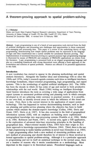
  • 8. 178 C J Webster remaining, the subgoal succeeds (that is, it is given the value True, and PROLOG moves on to the next clause in the rule, link(B,C,DistBC), which becomes the next subgoal. This is successfully matched with line 6, with X being instantiated to zone8 and DistBC to 4.6. PROLOG then makes add(DistAB,DistBC,DistAC) the next subgoal, which matches with line 2 and succeeds with distance instantiated to 7.8. At this point the main goal succeeds. The program does not stop, however, because PROLOG'S inference mechanism has a built-in backtracking algorithm which causes it to carry on searching for clauses that will match the goal. It tries to find another match for add(DistAB,DistBC,distance) and since there is none moves back to link(B,X,DistBC). A second match is found in line 7 and this subgoal therefore succeeds for the second time and PROLOG moves on once again to make add(DistAB,DistBC,DistAC) a subgoal which succeeds with the new instantiation for DistBC picked up from line 7. Backtracking within the goal continues until all possible matches for each of the subgoals on the right-hand side of the rule have been found, at which point PROLOG moves on to find any more matches for the goal among subsequent rules and facts. The search tree described by this process is given in figure 1 and shows that there are three solutions to the goal when it is matched with the rule in line 1. Once the search has finished backtracking through the rule, three further solutions are found when the goal is matched with the facts on lines 3, 5, and 8. link(zone1,X,distance):- linMzonelB.DistABJJinMBXDistBO.adcKDistAB.DistBCdistance). (1) (2) , (3) subgoal (1) succeeds with A=zone1, B=zone5 DistAB=3.2 subgoal (1) succeeds with A=zone1f B=zone2 DistAB-1.7 subgoal (1) succeeds with A=zone1, B=zone3 DistAB=5.0 subgoal (2) succeeds with B=zone5, X=zone8 DistBO=4.6 subgoal (3) succeeds with DistAB=3.2 DistBC=4.6 distance=7.8 goal succeeds with X==zone8 distance=7.8 subgoal (2) succeeds with B=zone2, X=zone8 DistBC=4.1 subgoal (3) succeeds with DistAB-1.7 DistBC=4.1 distance=5.8 goal succeeds with X=zone8 distance=5.8 subgoal (2) succeeds with B=zone5, X=zone12 DistBC=6.7 subgoal (2) fails since no match is found for the pattern: link(zone3,X,DistBC) subgoal (3) succeeds with DistAB=3.2 DistBC=6.7 distance=9.9 goal succeeds with X=zone12 distance=9.9 Figure 1. Search tree for a PROLOG rule.
  • 9. A theorem-proving approach to spatial problem-solving 179 The result of the program will be a listing of the instantiations given to the goal's variables at each success: X=zone8 distance=7.8 X=zone5 distance=3.2 X=zone12 distance=9.9 X=zone2 distance=1.7 X=zone8 distance=5.8 X=zone3 distance=5.0 From a theoretical point of view, this search pattern can be thought of as implementing theorem resolution in the following way. First, the Goal:- prompt is interpreted as a ~ and the goal is therefore introduced into the program as the negated clause: ~link (zonel,X, distance) . (25) Second, PROLOG searches for a matching clause by which to test the truth of clause (25). The first match, as we have seen, is with the rule in line 1 which in unnormalised form is link (A, C, DistAC) < = [link (A, B, DistAB) # link (B, C, DistBC) # add (DistAB, DistBC, DistAC)] , (26) and in partially normalised form is link (A, C, DistAC) # ~[link (A, B, DistAB) # link (B, C, DistBC) # add (DistAB, DistBC, DistAC)] . (27) Applying the resolution principle (20) to rule (27), we know that if rule (27) is true and ~link (A, C, DistAC) (28) is true then ~[link (A, B, DistAB) # link (B, C, DistBC) # add (DistAB, DistBC, DistAC)] (29) must be true. Since, as has been shown, the goal is equivalent to hypothesising clause (28) [with the variables in clause (28) instantiated to the values in the goal], then it follows that in order to prove the goal we will need to hypothesise clause (29). Hence clause (29) becomes a subgoal and the process of resolution repeats itself. In fact clause (29) becomes a series of subgoals since when fully normalised it breaks down into three separate clauses: ~link (A, B, DistAB) , (30) ~link(B, C, DistBC) , (31) ~add (DistAB, DistBC, DistAC) . (32) Each of these becomes a subgoal which in turn is resolved against matching clauses in the manner already described. The goal succeeds when an empty resolvant clause is generated, because this proves that the negated goal does not follow from the premises. Since there may be more than one clause with which to resolve the goal or a subgoal, several resolution paths are traced. In the example given, six nil resolvants are generated, (represented by the four PROLOG matches) demonstrating that there are six ways of proving that the hypothesis follows from the premises. Each proof is associated with a different set of instantiations and these become the output of the PROLOG program. Some more complex applications A summary of two rather more complex applications will illustrate the elegance of logic programming to spatial problem-solving. Chen (1986) describes a logic programming implementation of a geographic data base designed to support
  • 10. 180 C J Webster object-based query. His example demonstrates the structural and functional similarity between the relational data base model and the logic formalism of PROLOG (see also Malpas, 1987) and shows how the latter may be used to implement an object- oriented GIS. His data base, which is designed to store the essential components of an infrastructure planning problem, contains three types of geographic entity, plan, town, and cable, each represented by a predicate clause which may also be thought of as a relation: plan (cen—town, cable—code) , (33) town (town—name, x, y, population, area) , (34) cable (cable—code, unit—cost) . (35) The plan predicate holds the name of the town assigned to the centre of a communication network along with a code for the type of cable selected. The town predicate stores the name, location, and area of towns in the planning region, and cable records the unit cost of each cable-type. Rules for processing the information stored in this way are expressed as Horn clauses and implemented as PROLOG rules. The following example uses a predicate called network to establish a relationship between any particular town in the network and the central town. The relationship is found in terms of distance and cost of connecting cable: network(CEN_TOWNJOWN,DIST,COST):- plan(CEN__TOWN,CABLE_CODE), cable(CABLE_CODE,UNIT_COST), town(CEN_TOWN,X,Y, ),!, town(TOWN,X1;Y1 ), distance(DIST,X,XX1,Y1), COST is DIST*UNIT_COST, writeinetworMCEN—TOWNJOWN^IS^COSTD^ail. (36) The _ symbol means that the value of a variable in that position is immaterial when matching. The fail and ! symbols are PROLOG'S rogue control characters which render the language less than purely logical. The cut (!) prevents backtracking any further to the left and the fail always causes the goal to fail even if the far right of the rule has been reached successfully, so that further solutions are sought. The write predicate causes the values in the parenthesised clause to be written to the screen. Rule (36) supports queries about any of the four variables making up the network predicate. To find the cost of installing a communication cable from Keluang to a number of other towns requires the hypothesis network(Keluang,TOWN,_,COST) to be negated and resolve against the rule above and the associated facts. This is implemented by entering the predicate in response to the goal prompt: Goal:-network(Keluang,TOWN COST) (37) Resolution of this predicate would return a list of instantiations for the variables TOWN and COST: for example, TOWN=Gajah COST=80000 TOWN=Paloh COST=110000 TOWN=Chaah COST=200000 TOWN=Bekok COST=180000 A second example comes from the familiar polygon-overlay problem arising in sieve mapping and other multiple map processing exercises. Franklin and Wu (1987)
  • 11. A theorem-proving approach to spatial problem-solving 181 describe a topological data base written in PROLOG and capable of vector-overlay processing. The fundamental data structure is a chain predicate containing variables for chain identifier (C), start and end nodes (N1, N2), left and right polygons (P1, P2) and X and Y coordinates. The latter are stored as a dynamic linear list (a built-in PROLOG data-type) which is identified by a single symbol in the predicate definition: chain(C,N1,N2,XYLIST,P1,P2) (38) There are three stages to the overlay process: chain intersection, polygon formation, and overlay identification. The second of these illustrates how a nontrivial process normally expressed in procedural algorithmic terms is defined declaratively in PROLOG predicates. After the chains from two maps have been intersected to produce a new and more numerous set of nodes and smaller chains, each of these chains is examined to identify the node at its head and tail. For each node, the chains that meet at that node are identified, sorted, and entered as PROLOG facts of the following type: node(Node,[Chain1,Chain2,Chain3,...]) (39) where Chainl, Chain2, etc are chain identifiers stored as head or tail predicates structured as a linear list. The following node predicate, for example, indicates that the heads of chains 18 and 21 and the tails of chains 19 and 24 come together at node 6 (figure 2): node(6,[h(18),t(19),t(24),h(21)]) (40) Since the list elements are in cyclical order, each consecutive pair defines a corner of an output polygon and this information is asserted as a new set of facts about linkage with the general structure: linkage([Chain1,Chain2]) (41) The node predicate above gives rise to four such facts (there are four corners at node 6): linkage([ht(19),ht(18)]). Iinkage([ht(24),th(19)]). Iinkage([th(21)fth(24)]). Iinkage([th(18)fht(21)]). (42) (43) (44) (45) polygon(1,[ht(18),ht(19)]) polygon(2,[ht(6),th(14),th(15)]) polygon(3,[th(6).th(12),ht(10)]) polygon(4,[th(5),ht(9),ht(12)]) polygon(5,[ht(11),th(9)]) polygon(6,[ht(5),ht(15)fth(18),ht(21),ht(25)]) polygon(7,[th(21),th(24)]) polygon(8f[ht(24),th(19),ht(14),th(10),th(11),th(25)]) Figure 2. The process of linking chains to form polygons.
  • 12. 182 C J Webster Three more nodes are represented similarly by the following node and linkage facts: node(5,[h(14),h(19),t(18),t(15)]) linkage([th(19),ht(14)]) linkage([ht(18);ht(19)]) linkage([ht(15),th(18)]) linkage([th(14),th(15)]) node(4,[t(12),h(6),h(15),t(5)]) linkage([th(6),th(12)]) linkage([th(15),ht(6)]) linkage([ht(5),ht(15)]) linkage([ht(12),th(5)]) linkage([th(6),th(12)]) node(2,[t(10),t(14),t(6)]) linkage([ht(14),th(10)]) linkage([ht(6),th(14)]) linkage([ht(10),th(6)]) (46) (47) (48) (49) (50) (51) (52) (53) (54) (55) (56) (57) (58) (59) (60) Predicates ht(Chain) and th(Chain) are simply renamed predicates h(Chain) and t(Chain), respectively, indicating explicitly the correct cyclical order in the formation of the corner (for example, the first corner is formed by following chain 19 from head to tail and then chain 18 from head to tail). The final step in forming output polygons is to concatenate the linkage facts in correct cyclical order. This entails searching for facts in which the second-list element of one matches with the first-list element of the other. Matching continues in this way until the second-list element in the most recent fact in the sequence matches with the first-list element in the first fact in the sequence. At that point the polygon has been closed and the search can go on to build another polygon. In the collection of facts above, there are two such complete sequences of chained linkage, facts (42) and (48) which define polygon 1, and (59), (50), and (53) which define polygon 2. Once a closed chain of linkages has been matched, a polygon fact is asserted, in the case of polygon 2, for example, polygon(2,[ht(6),th(14),th(15)]) (61) The simplicity of processing in a declarative programming environment such as this is illustrated by the rule which generates a polygon fact from the linkage facts: makepolygon(PolyNumber,X,Y):- linkage([X,Y]), linkage([Y,Z]), addToList(X,Y,Z,[H|T]), retract(polygon(PolyNumber,_), asserta(polygon(PolyNumber,[H|T])), setPolyNumber(PolyNumber), ZOH, makepolygon(PolyNumber,Y,Z). (a linkage fact can be found) (a second linkage fact can be found whose list head matches the list tail of the first fact) (add X,Y, and Z to a dynamic list) (retract any previously stored polygon predicates of this number) (store this polygon predicate with its updated list) (call a predicate which increments Polynumber by 1 if Z=H) (check for close of polygon) (call makepolygon recursively to repeat the search this time with the second fact as the fact to be matched against). (62)
  • 13. A theorem-proving approach to spatial problem-solving 183 Advantages of a logic programming approach Logic programming has been associated by some with the dawn of a new computing age. Such proponents have tended to see it as a completely new way of articulating a problem; as a methodological innovation offering a novel, elegant, and mathematically based method of structuring and solving problems. It was viewed in this way by the Japanese who chose it as the genus of language for their fifth- generation computer initiative (Moto-oka, 1985). Others have been more cautious and greeted it merely as another programming lanaguage (Jackson, 1986). The advantages that the approach offers to those concerned with managing and processing data can be usefully summarised under two headings: user-data interface and data- knowledge structuring. Underlying both is its strong relationship to theory. First, it presents a particular kind of interface between programmer or program- user and data. At the broadest level, and in common with many other new-generation programming tools, it offers a very high-level view of a problem. Its declarative and pattern-matching nature means that the use of natural-language style predicate and variable identifiers also means a natural-language style of command syntax. This is in contrast to the use of meaningful identifiers in conventional structured languages which are, in effect, merely useful notation for the programmer. A feature which is unique to logic programming among the high-level languages is its semantic flexibility. A logic clause can be issued in the declarative, in which case it is interpreted as the assertion of a truth. Alternatively, it may be issued in the imperative, in which case it is interpreted as a command. As we have seen, a clause used in the imperative returns either the truth of the clause, or, if it contains variable names, its truth plus the values given to those variables during successful matches. The benefit that such flexibility brings is the ability to make deductive queries such as those illustrated, which are of a style not possible in other data- processing environments. Second, the primary data model which logic programming rigidly imposes both on data and on procedures gives certain advantages. The Horn clause is, in essence, a very simple structure. To break down a problem into a series of antecedent IF precedent rules supported by a series of single predicate facts is an appealingly simple approach. In principle, it should give a program a more reasonable flavour and make it easier to follow and to adapt. Even with a complex program in which there is not an obvious one-to-one mapping of steps of intuitive reasoning to predicates and rules, there is still a simplicity of structure which makes adaptation relatively straightfoward. One aspect of this is the simplicity of tracing through the logic of a program; done by matching one clause to another. Another is the ease with which axioms can be added or removed. A new rule or fact can, in principle, simply be added to the end of a program, in the same way as a tuple (record) can be appended to the end of relation in a relational data base (RDB). Amending facts in this way does not interrupt the logic of the rest of the program; adding rules does but does not require the existing program to be rewritten in any way. The similarity with relational data bases is more than superficial; RDB theory has the same mathematical roots as logic programming (Gallaire and Minker, 1978). One advantage this brings is that logic programming can be thought of as directly supporting not only a predicate logic data model but also a relational model because relations can easily be mapped into predicate clauses. Its link with relational theory is perhaps of more practical benefit to many users than its link to resolution theory. The latter, for most users, will remain an underlying theoretical basis which establishes the soundness of the approach but is not explicitly articulated in the process of design. As we have seen, logic programming allows a programmer to think in terms of matching rather than resolution. It is unlikely that users in
  • 14. 184 C J Webster our field will program in logic because of the need to establish the logical veracity of a program. (This was an important motivation behind the original development of the language and related to the need to test programs designed for the control of nuclear installations and other sensitive plant.) A final advantage of logic programming's method of data structuring derives from its symbolic nature. This is its ability to handle with equal ease hard and soft information. This is obviously of particular significance in a field in which opinions, expectations, heuristics, fuzzy reasoning, and other imprecise measurables are as important to the analyst as more precise numerical relationships. It is, in essence, a symbolic processing system where the processing concerns testing hypotheses about relationships between symbols and where symbols may represent any type of data item. Thus, symbolised expectations can be processed as easily as real numbers and relationships can be expressed in rules of thumb as easily as in mathematical equations. The popularisation of logic programming in our field is likely to be driven by two forces. One is the general evolution of state-of-the-art programming in mainstream computer science. Accepted programming practice is rapidly evolving there and we should expect such developments to filter through into applied areas like our own. This process is probably a slow one in reality given the lack of time for retooling and other factors leading to inertia in skill-upgrading. The other and more important factor is the pressure to develop programs and systems with smart features. Intelligence is a buzzword that will not go away and the next decade will see the further demise of conventionally designed data-processing systems in favour of knowledge-based systems. Logic programming along with its cousins such as object-oriented programming, fourth-generation languages, and multipurpose knowledge-engineering environments are the problem-solving tools of the future and this will have an influence on the general expectations made of software. The pressure on the academic community to modernise in this respect will grow in line with the pressure to sell its analytical skills [for a classic illustration of the pressure on UK academic planners and geographers to commercialise see Masser's (1987) summary of the ESRCs Regional Research Laboratory initiative]. It can be enormously inefficient to write intelligent systems in conventional languages; logic programming, on the other hand, is a natural language for such tasks. It is possible to identify a number of areas in which logic programming is likely to be applied in our field. First, there is the type of application which explores the benefits of articulating familiar problems in a logic framework. Franklin and Wu's (1987) polygon-overlay program is an example. It can be expected that this sort of work will give insight into established algorithms and will yield new algorithms: semantically oriented algorithms, better suited to the programming environment of the next decade. Second, there is the design of prototype and experimental expert systems and other rule-based decision-support systems. This will be of particular importance in qualitative analysis and it may be supposed that tools such as logic programming, representing, as we have seen, a paradigm as well as a language, may give new directions to the development of qualitative analytical techniques. Diamond and Wright (1988), for example, explore a fresh approach to the site-screening decisionmaking process by using a rule-based expert system to add intelligence to a system that combines a GIS and multiobjective programming model. This highlights a third area of application, namely the design of intelligent front- ends to conventional systems. This will be important where fresh ways of interacting with an established data base are required and also where several systems need to be accessed through a single interface. It will also be important in bringing GIS
  • 15. A theorem-proving approach to spatial problem-solving 185 into the intelligent age. The large volumes of data stored within a GIS and the specialised data structures required have acted as a barrier to the penetration of relational data-base technology into GIS during 1980s, with only the attribute data typically being stored as relations and topographic data being held in specialised file structures. The same sort of constraints are likely to be encountered during the 1990s as GIS attempts to establish a relationship with knowledge-based technology. Franklin and Wu's work described earlier in this paper does in fact structure topographic data within a rule-based system, but this is unlikely to be practicable for large real-world systems given current serial processing technology. Intelligent GIS systems will therefore employ front-end processors constructed as expert-system, natural-language parsers and graphics pattern-recognition systems written in logic programming and similarly appropriate languages. Given the current interest in the relational model a fourth type of application is likely to be in implementing various kinds of relational data-management systems such as relational interfaces to nonrelational GIS (Ingram and Phillips, 1987) and relational models of socioeconomic processes (Seidman, 1987). It seems possible, however, that relational data-base applications may be overtaken by developments in postrelational data-processing technology, since semantic-oriented approaches look set to supersede the relational approach as the flavour of the moment. This is particularly so in the GIS field where the semantic approaches seem more suited to the nature of geographic data than the relational approaches (Gahegan and Roberts, 1988). Logic programming will survive this shift in fashion, however, because as well as having an affinity to relational theory, its built-in control mechanism renders it particlarly suited to implementing the inheritance functionality which is central to object-oriented approaches (Zaniolo, 1984). References Black W J, 1986 Intelligent Knowledge-based Systems (Van Nostrand Reinhold, Wokingham, Berks) Charniak E, McDermott D, 1985 Introduction to Artificial Intelligence (Addison-Wesley, Reading, MA) Chen G, 1985, "The design of a spatial database management system", in Proceedings, Auto Carto 7 held in Washington, DC (American Society of Photogrammetry and Remote Sensing and American Congress on Surveying and Mapping, Falls Church, VA) pp 423-432 Chen G, 1986, "A rule-based approach for spatial object modelling and task management", in Proceedings, Auto Carto London held 14-19 September, London (Auto Carto London Ltd and Royal Institute of Chartered Surveyors, London) pp 588-597 Chikayama T, 1983, "ESP—extended self-contained Prolog—as a preliminary kernel of fifth generation computers" New Generation Computing 1 11-24 Clark K L, Gregory S, 1985, "Notes on the implementation of PARLOG" Journal of Logic Programming 2 17-42 Clocksin W F, Mellish C G, 1984 Programming in Prolog 2nd edition (Springer, Berlin) Cullen I, 1986, "Expert systems in planning analysis" Town Planning Review 57 239-251 Davis J R, Grant I W, 1987, "ADAPT: a knowledge-based decision support system for producing zoning schemes" Environment and Planning B: Planning and Design 14 53-66 Davis J R, Compagnoni P T, Nanninga P M, 1987, "Roles for knowledge-based systems in environmental planning" Environment and Planning B: Planning and Design 14 239-254 Diamond J T, Wright J R, 1988, "Design of an integrated spatial information system for multiobjective land-use planning" Environment and Planning B: Planning and Design 15 205-214 Franklin W R, Wu P Y F, 1987, "A polygon overlay system in prolog", in Proceedings, Auto Carto 8 held in Baltimore, MD, 29 March-3 April (American Society of Photogrammetry and Remote Sensing and American Congress on Surveying and Mapping, Falls Church, VA)pp 97-106 Franklin W R, Wu P Y F, Samaddar S, Nichols M, 1986, "PROLOG and geometry projects" IEEE Computer Graphics and Applications 6 46-55
  • 16. C J Webster Gahegan M N, Roberts S A, 1988, "An intelligent, object-oriented geographica information system" International Journal of Geographic Information Systems 2 101-110 Gallaire H, Minker J (Eds), 1978 Logic and Data Bases (Plenum Press, New York) Gonzalez J C, Williams M H, Aitchinson I E, 1984, "Evolution of the effectiveness of PROLOG for a CAD application" IEEE Computer Graphics and Applications 4 67-75 Ingram K J, Phillips W W, 1987, "Geographical information processing using an SQL based query language" Proceedings, Auto Carto 8 held in Baltimore, MD, 29 March-3 April (American Society of Photogrammetry and Remote Sensing and American Congress on Surveying and Mapping, Falls Church, VA) pp 326-335 Jackson P, 1986 Introduction to Expert Systems (Addison-Wesley, Reading, MA) Lloyd J W, 1984 Foundations of Logic Programming (Springer, New York) Malpas J, 1987 PROLOG: A Relational Language and its Applications (Prentice-Hall, Englewood Cliffs, NJ) Marcus C, 1986 Prolog Programming (Addison-Wesley, Reading, MA) Masser I, 1987, "The regional research laboratory initiative: the experience of the trial phase", Economic and Social Research Council, Cherry Orchard East, Kembrey Park, Swindon SW2 6UQ, Wilts Moto-oka T, 1985, "Challenge for knowledge information processing systems", in The Fifth Generation Computer: The Japanese Challenge (John Wiley, New York) pp 3-92 Muller J C, Johnson R D, Vanzella L R, 1986, "A knowledge-based approach developing cartographic expertise", in Proceedings, 2nd International Symposium on Spatial Data Handling held in Seattle, WA (International Geographical Union, Williamsville, NY) pp 557-571 Robinson J A, 1965, "A machine-oriented logic based on the resolution principle" Journal of the ACM 12 23-41 Robinson V B, Frank A U, 1987, "Expert systems applied to problems in geographic information systems", in Proceedings, Auto Carto 8 held in Baltimore, MD, 29 March-3 April (American Society of Photogrammetry and Remote Sensing and American Congress on Surveying and Mapping, Falls Church, VA) pp 510-519 Seidman S B, 1987, "Relational models for social systems" Environment and Planning B: Planning and Design 14 135-148 Shafer D, 1987 Advanced Turbo Prolog Programming (Howard W Sams, Indianapolis, IN) Simmons R F, 1984 Computations from the English (Prentice-Hall, Englewood, Cliffs, NJ) Winston P H, 1984 Artificial Intelligence 2nd edition (Addison-Wesley, Reading, MA) Zaniolo C, 1984, "Object-oriented programming in Prolog", in Proceedings, International Symposium on Logic Programming held in Atlantic City, NJ, 6-9 February (IEEE Computer Society Press, New York) pp 265-271 p © 1989 a Pion publication printed in Great Britain