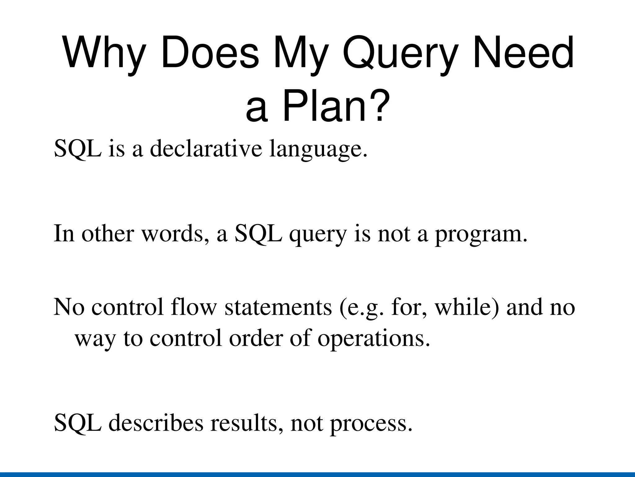
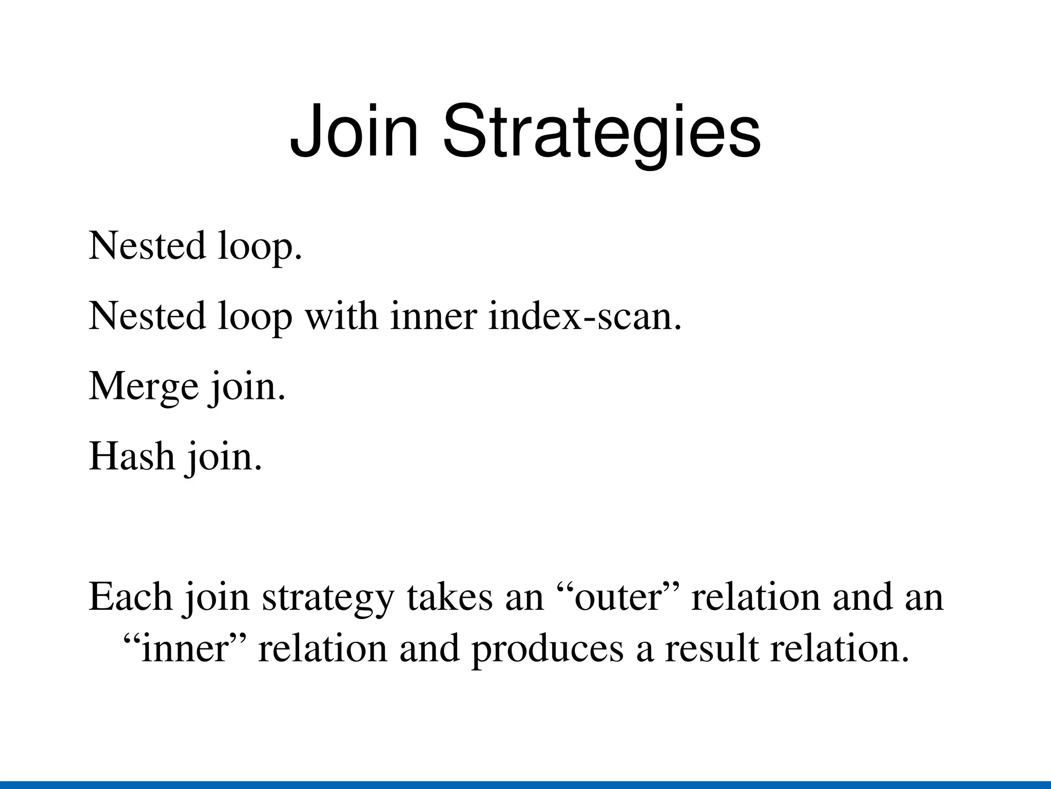
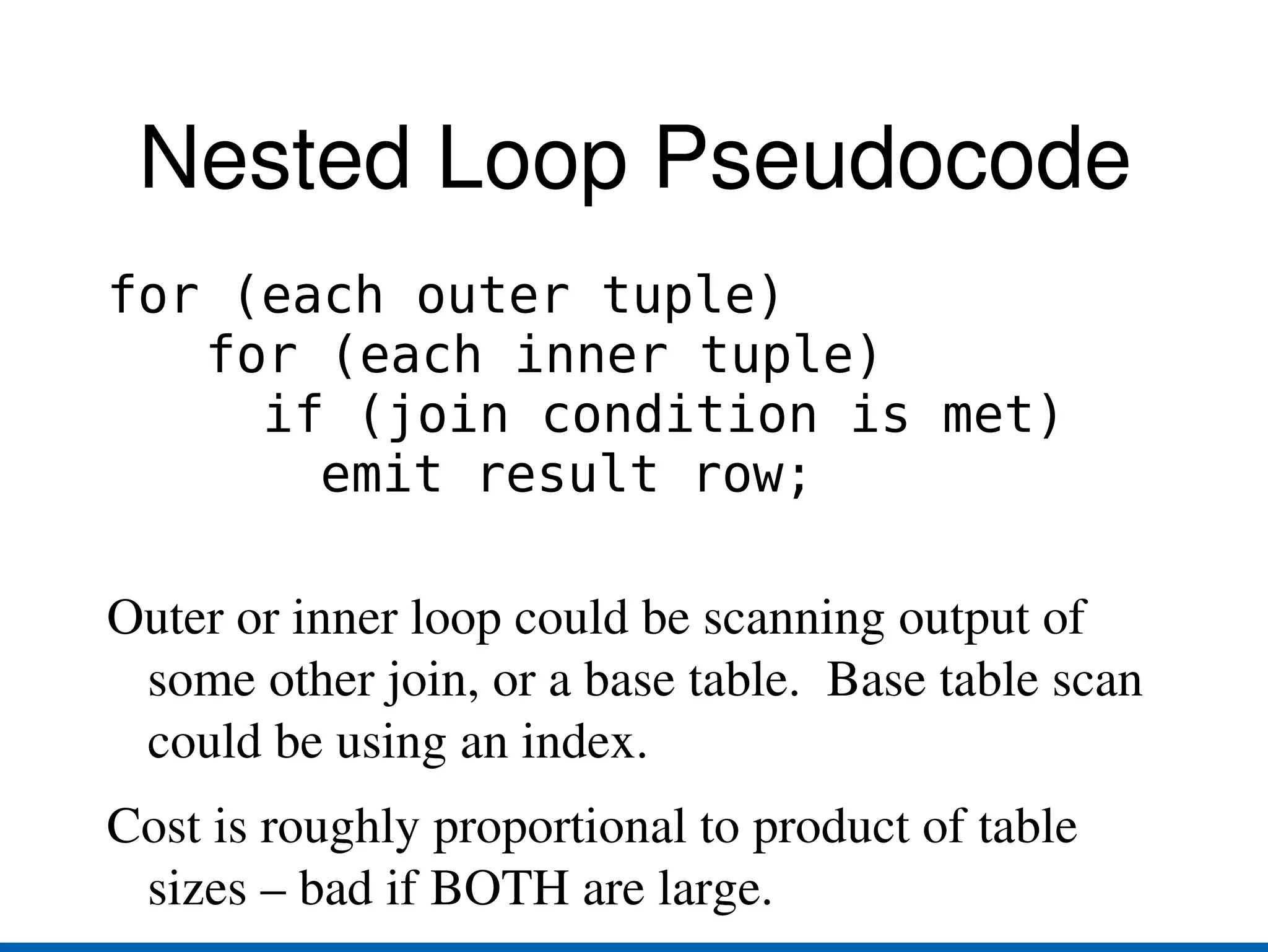
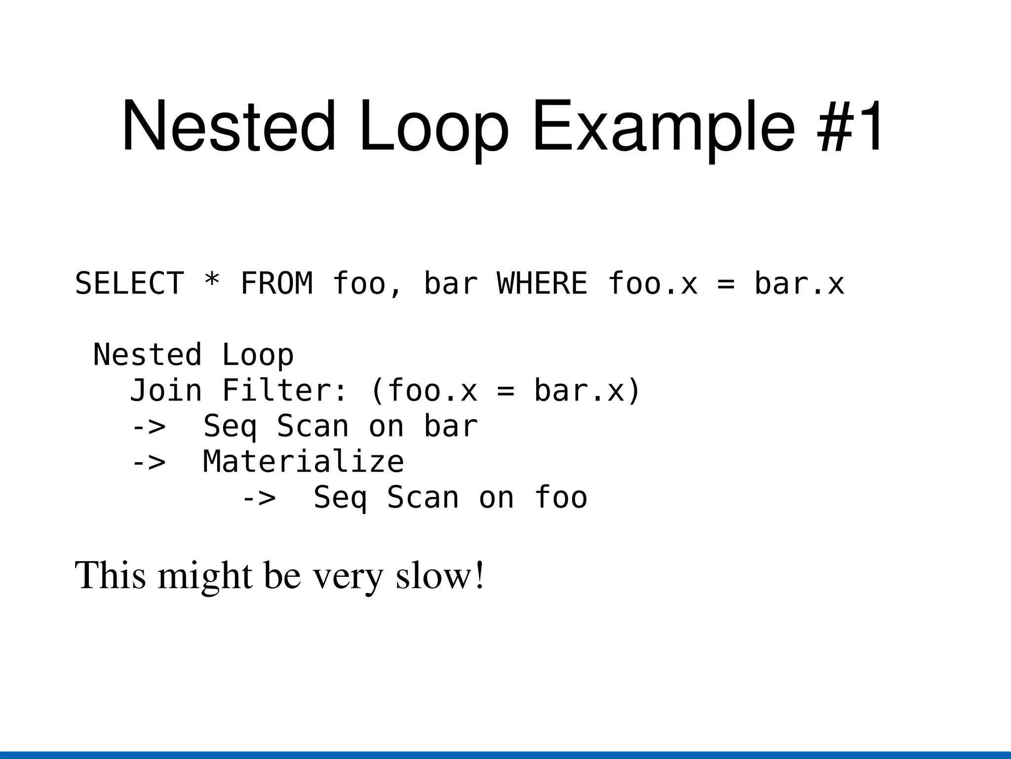
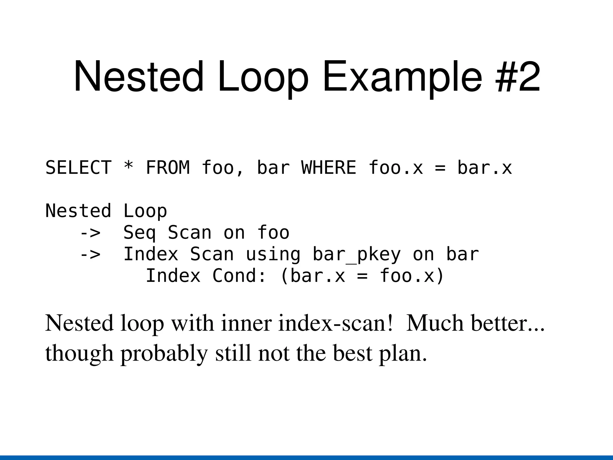
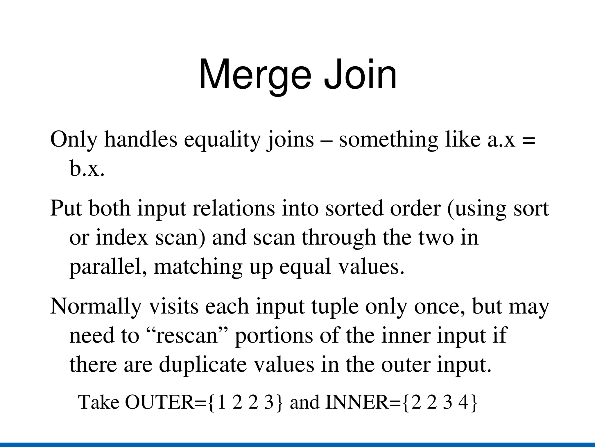
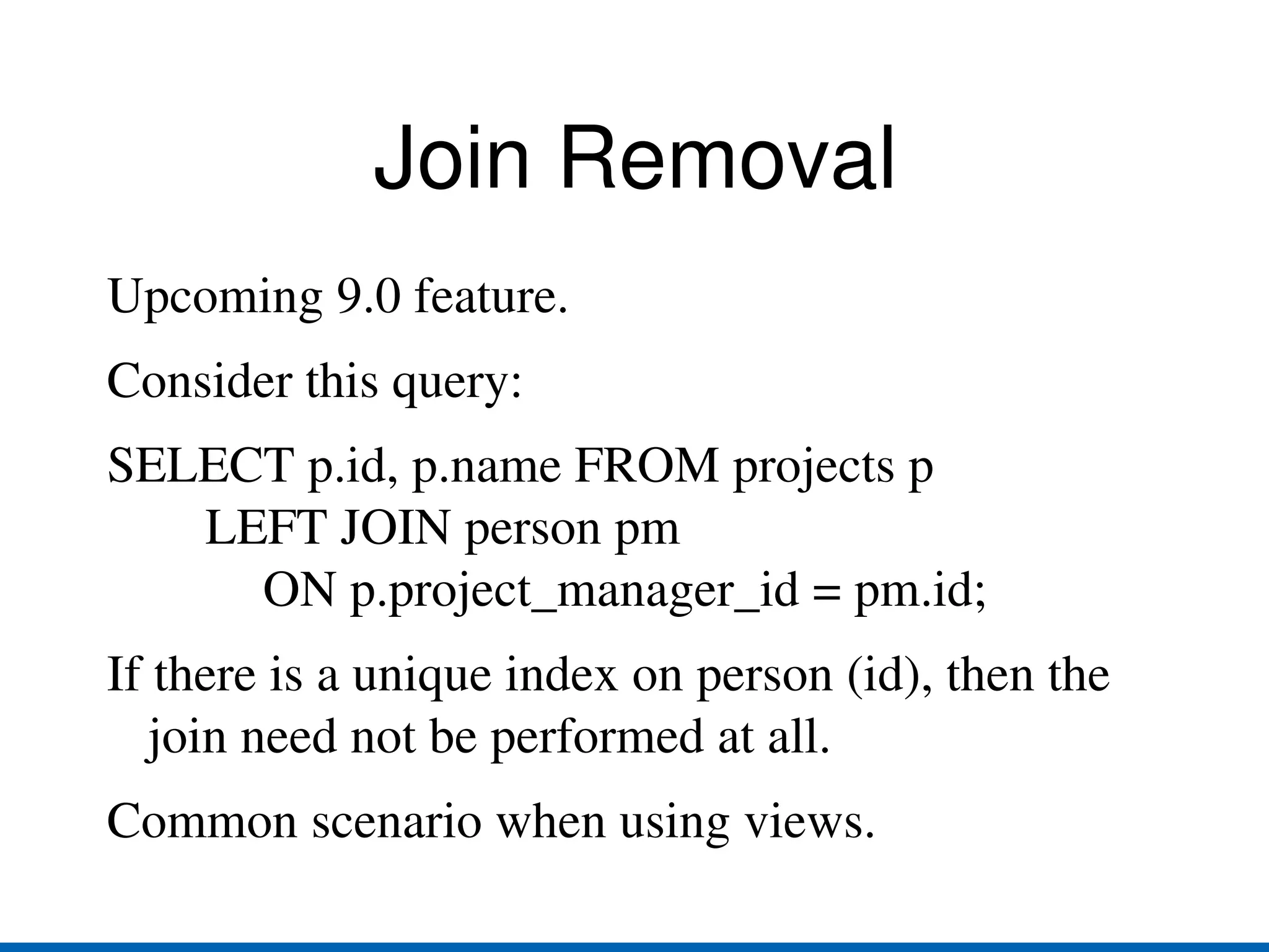
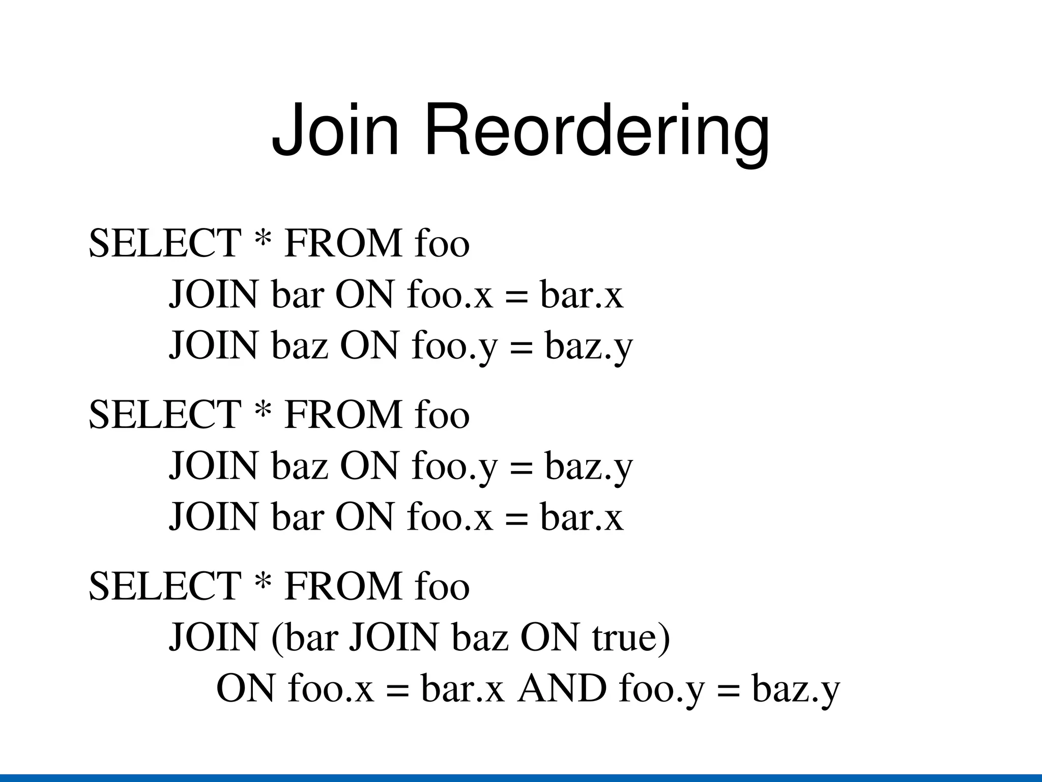
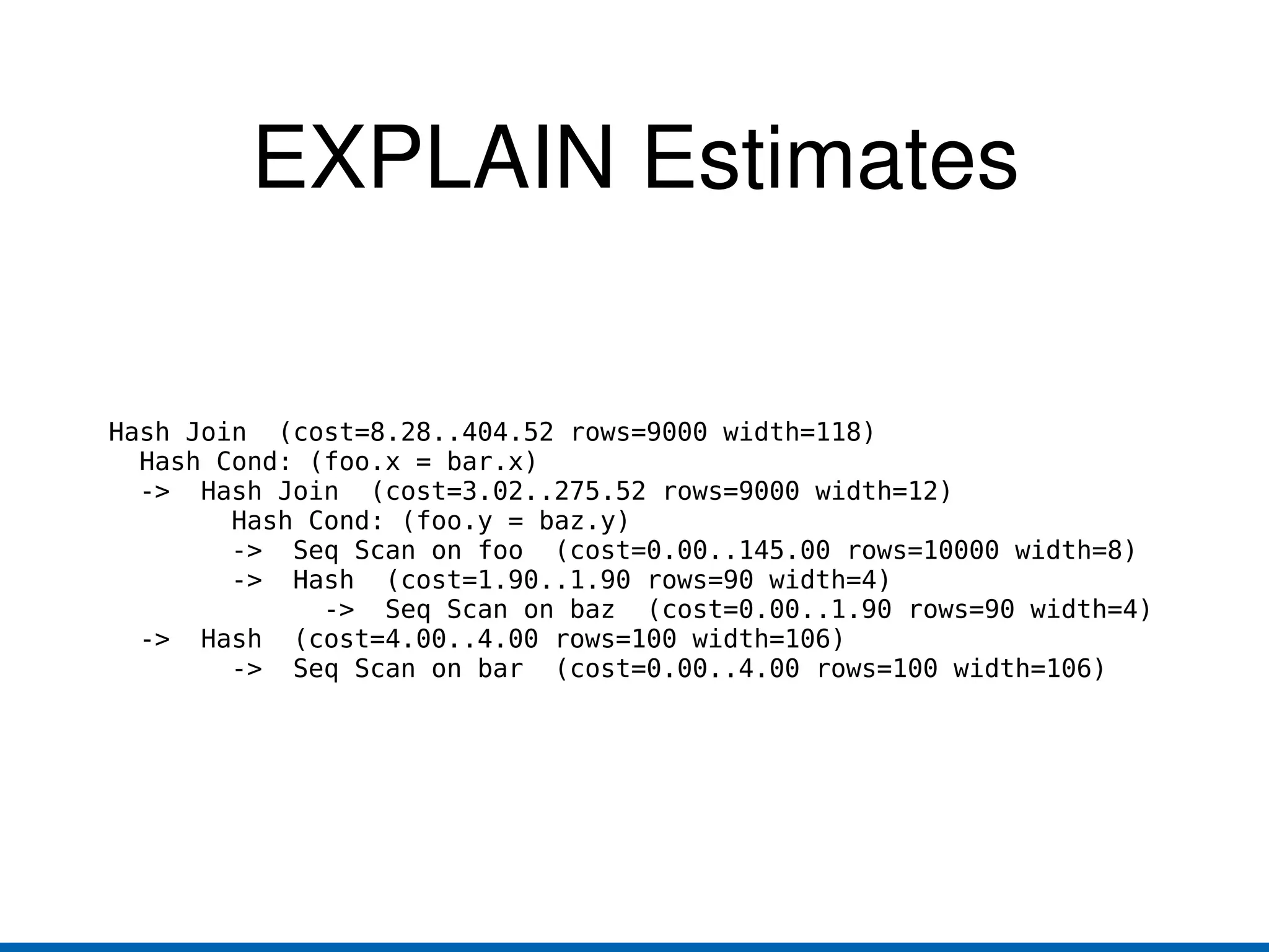
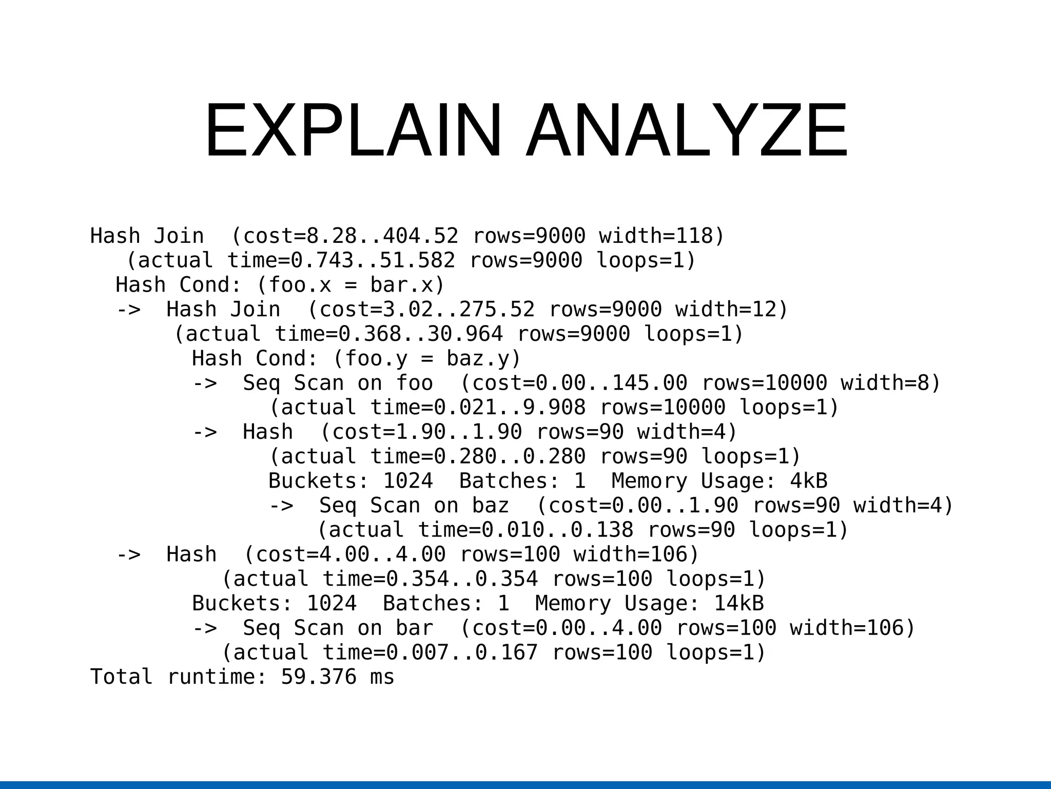
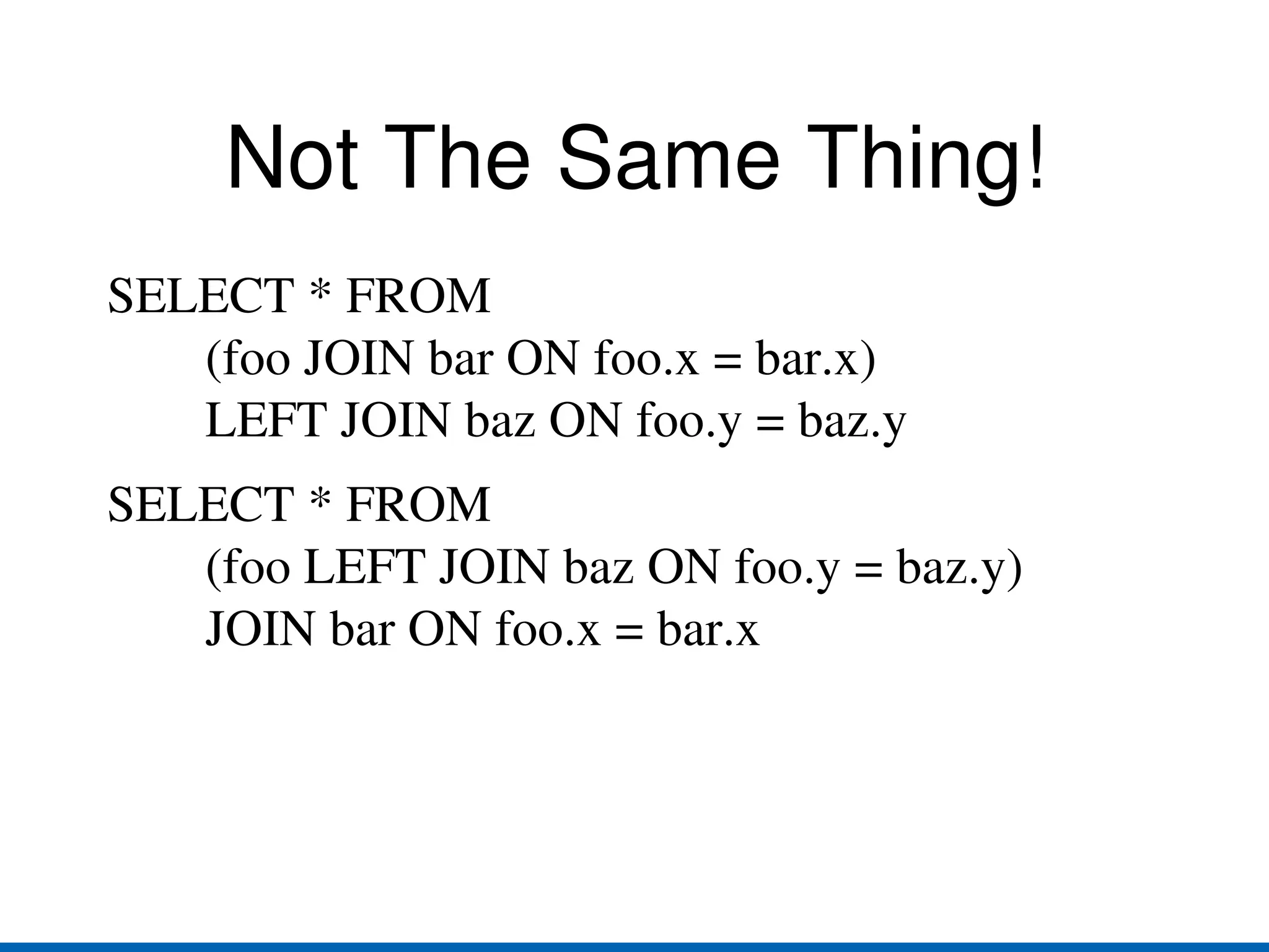
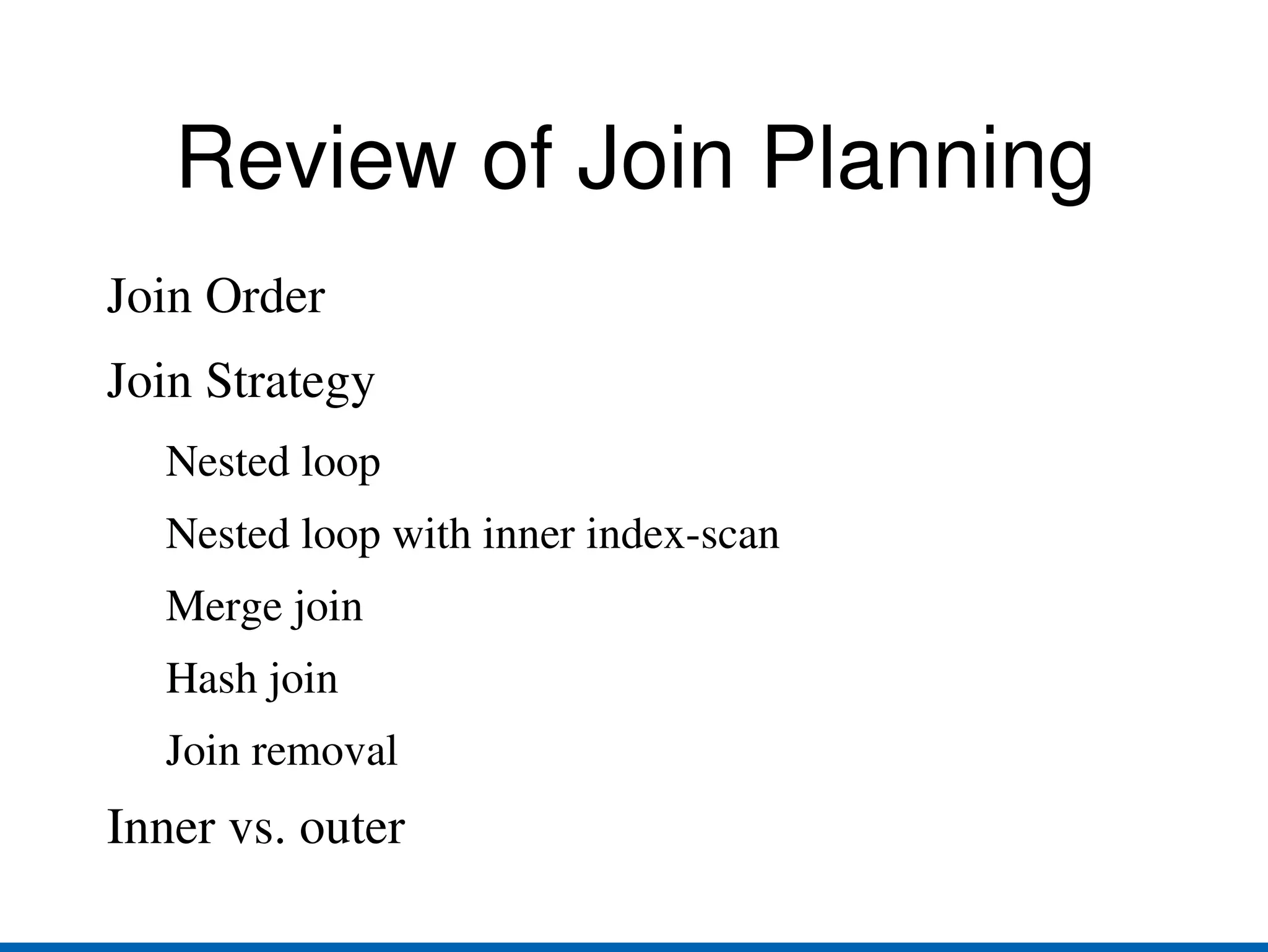
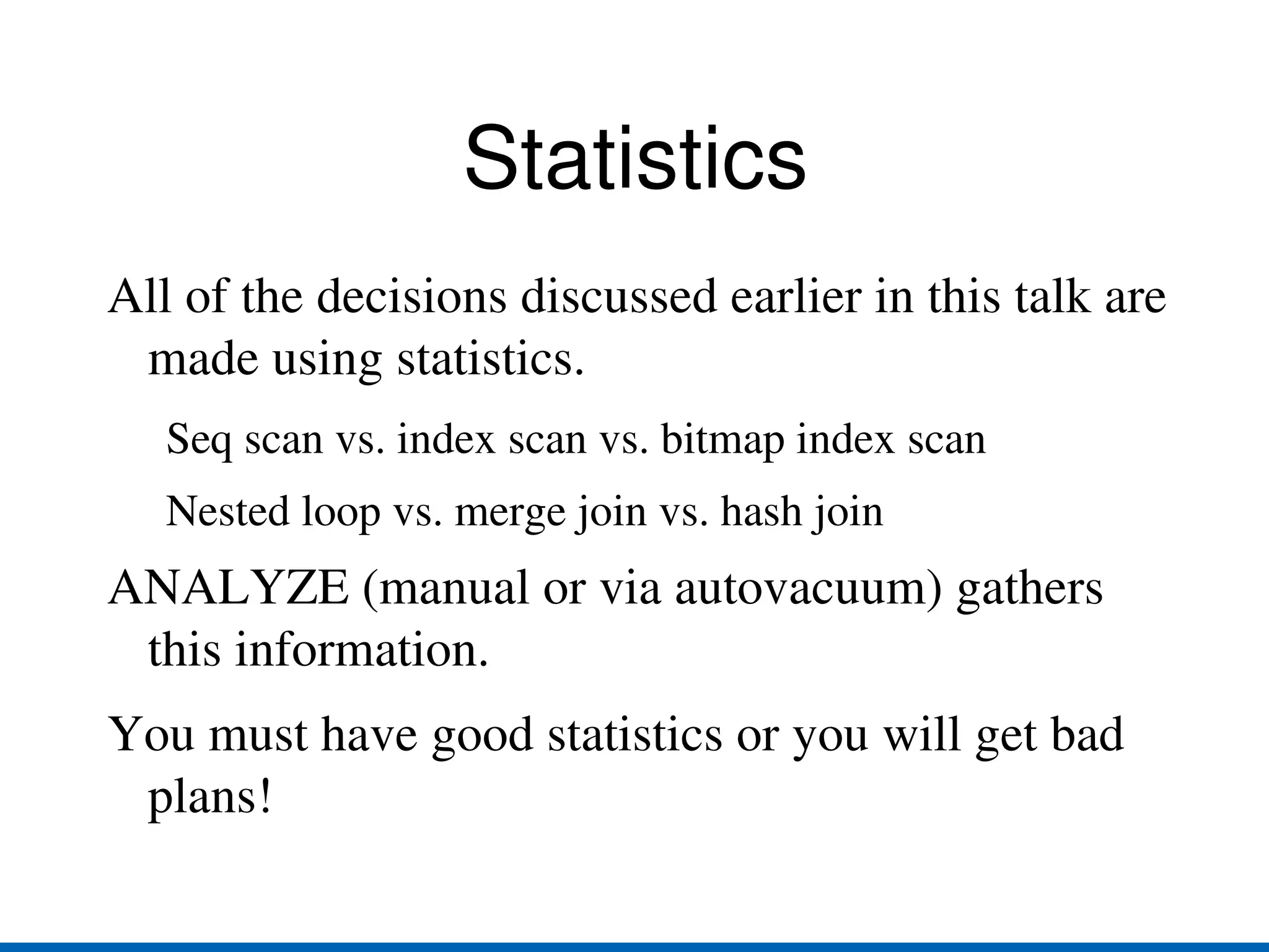
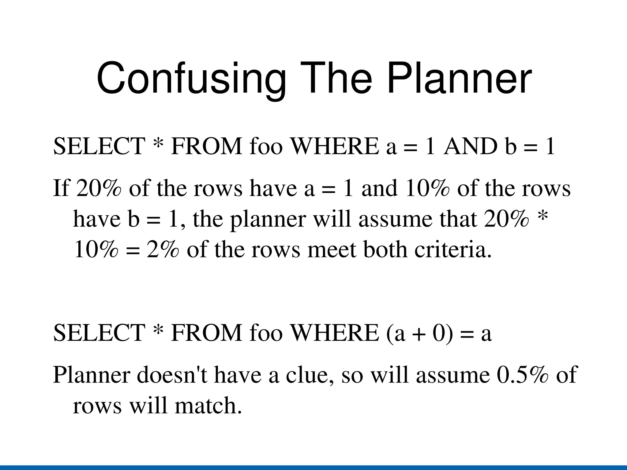
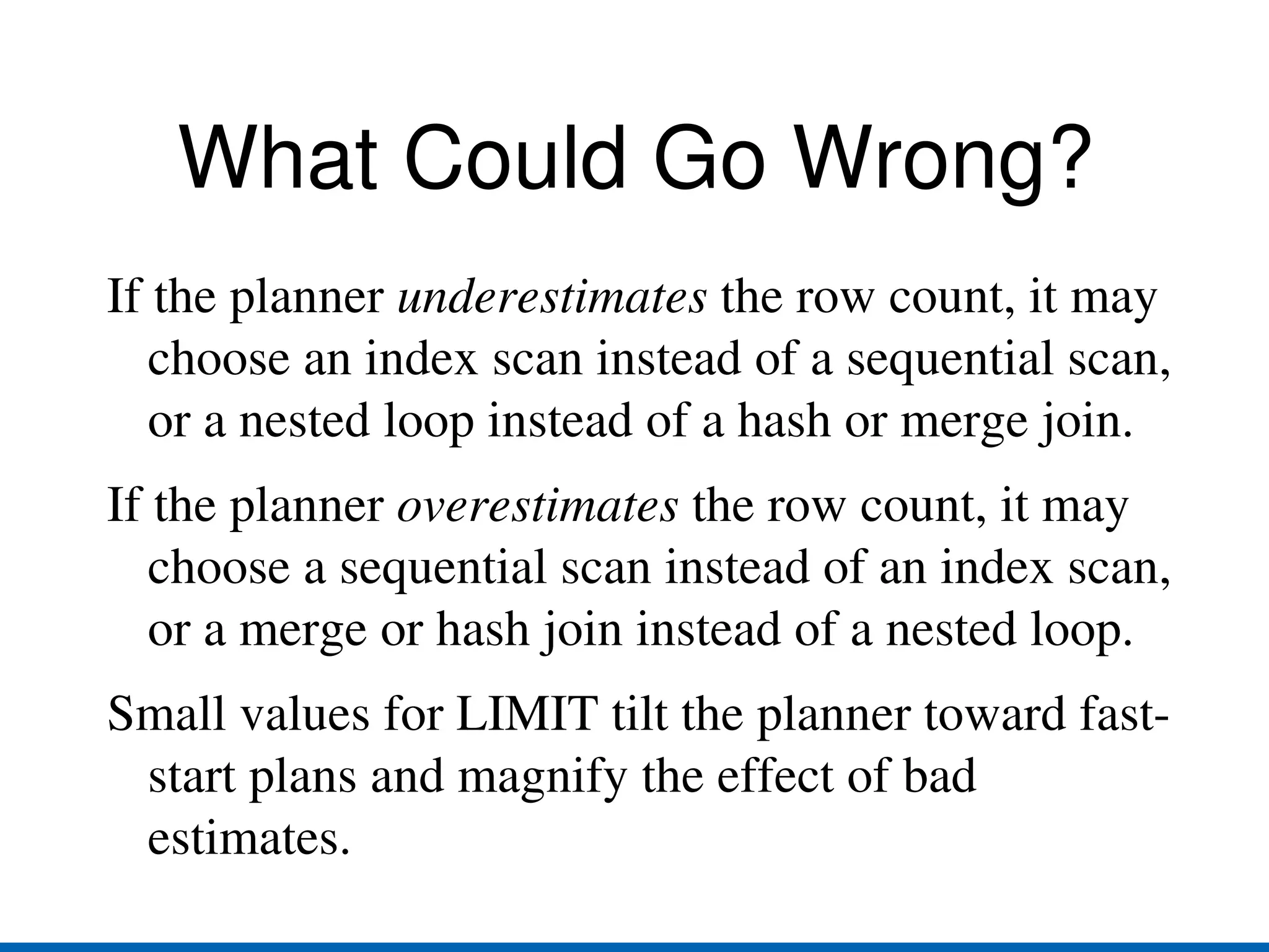
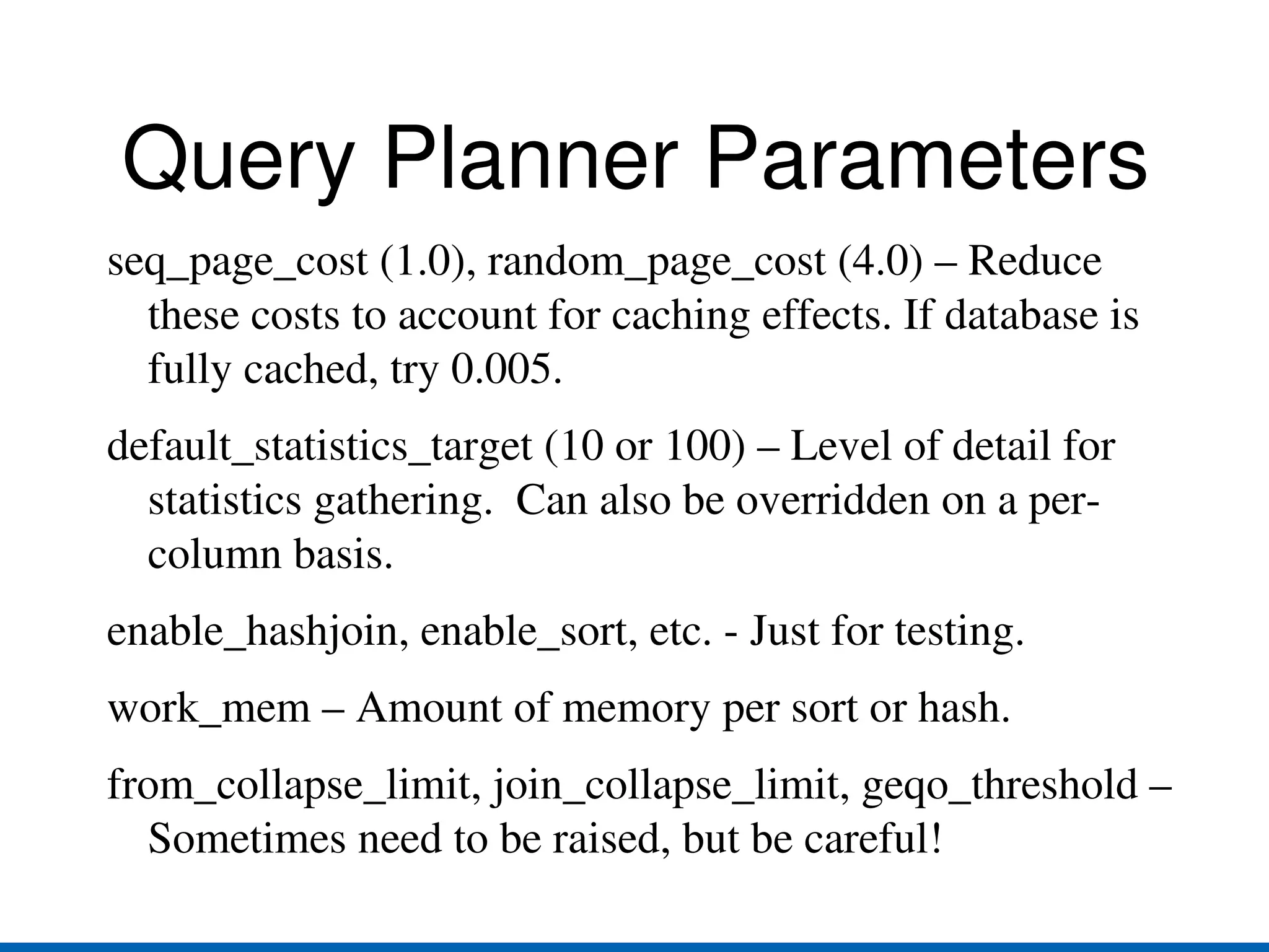
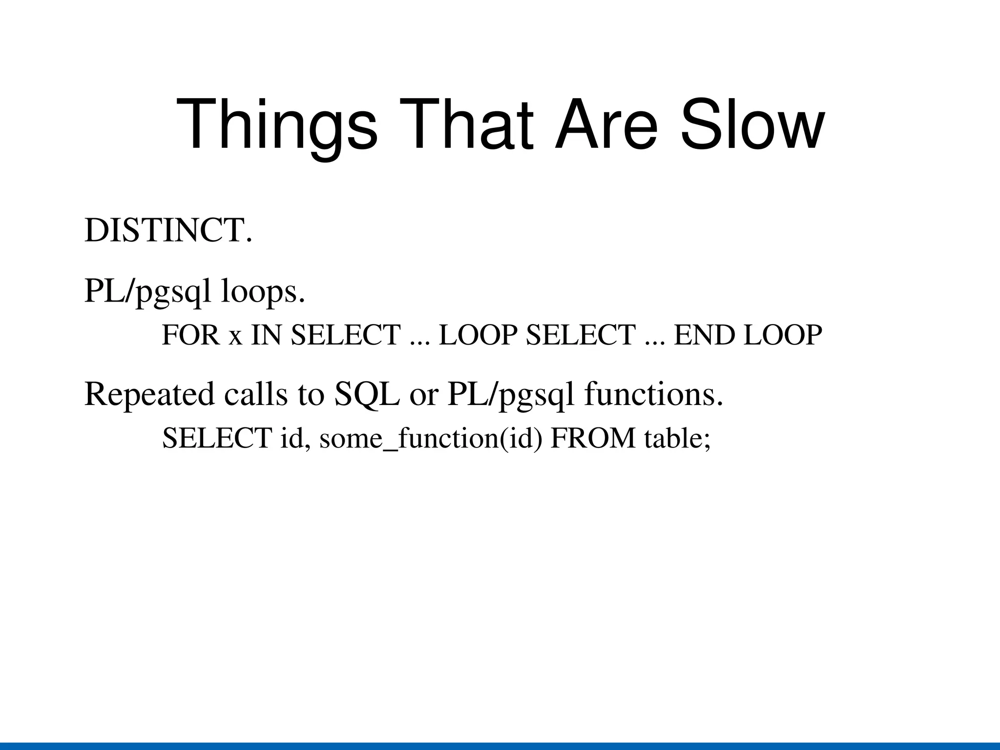
The document discusses the PostgreSQL query planner, detailing the importance of query planning for optimizing SQL queries' performance by minimizing disk I/O and CPU usage while ensuring correct results. It explains different access and join strategies, such as sequential scan, index scan, nested loop, merge join, and hash join, along with considerations for join order and strategy selection based on table statistics. The document also highlights common pitfalls in query planning due to inaccurate statistics and the upcoming features aimed at improving query optimization.

1. The PostgreSQL Query Planner Robert Haas PostgreSQL East 2010

2. Why Does My Query Need a Plan? SQL is a declarative language.

3. In other words, a SQL query is not a program.

4. No control flow statements (e.g. for, while) and no way to control order of operations.

5. SQL describes results, not process.

6. Why Didn't The Planner Do It My Way? Maybe your way is actually slower, or

7. Maybe you gave the planner bad information, or

8. Maybe the query planner really did goof.

9. Related question: How do I force the planner to use my index?

10. Query Planning Make queries run fast. Minimize disk I/O.

11. Prefer sequential I/O to random I/O.

12. Minimize CPU processing. Don't use too much memory in the process.

13. Deliver correct results.

14. Query Planner Decisions Access strategy for each table. Sequential Scan, Index Scan, Bitmap Index Scan. Join strategy. Join order.

15. Join strategy: nested loop, merge join, hash join.

16. Inner vs. outer. Aggregation strategy. Plain, sorted, hashed.

17. Table Access Strategies Sequential Scan (Seq Scan) Read every row in the table. Index Scan or Bitmap Index Scan Read only part of the table by using the index to skip uninteresting parts.

18. Index scan reads index and table in alternation.

19. Bitmap index scan reads index first, populating bitmap, and then reads table in sequential order.

20. Sequential Scan Always works – no need to create indices in advance.

21. Doesn't require reading the index, which has both I/O and CPU cost.

22. Best way to access very small tables.

23. Usually the best way to access all or nearly the rows in a table.

24. Index Scan Potentially huge performance gain when reading only a small fraction of rows in a large table.

25. Only table access method that can return rows in sorted order – very useful in combination with LIMIT.

26. Random I/O against base table!

27. Bitmap Index Scan Scans all index rows before examining base table, populating a TID bitmap.

28. Table I/O is sequential, with skips; results in physical order.

29. Can efficiently combine data multiple indices – TID bitmap can handle boolean AND and OR operations.

30. Handles LIMIT poorly.

31. Join Planning Fixing the join order and join strategy is the “hard part” of query planning.

32. # of possibilities grows exponentially with number of tables.

33. When search space is small, planner does a nearly exhaustive search.

34. When search space is too large, planner uses heuristics or GEQO to limit planning time and memory usage.

35. Join Strategies Nested loop.

36. Nested loop with inner index-scan.

37. Merge join.

38. Hash join.

39. Each join strategy takes an “outer” relation and an “inner” relation and produces a result relation.

40. Nested Loop Pseudocode for (each outer tuple) for (each inner tuple) if (join condition is met) emit result row; Outer or inner loop could be scanning output of some other join, or a base table. Base table scan could be using an index.

41. Cost is roughly proportional to product of table sizes – bad if BOTH are large.

42. Nested Loop Example #1 SELECT * FROM foo, bar WHERE foo.x = bar.x Nested Loop Join Filter: (foo.x = bar.x) -> Seq Scan on bar -> Materialize -> Seq Scan on foo This might be very slow!

43. Nested Loop Example #2 SELECT * FROM foo, bar WHERE foo.x = bar.x Nested Loop -> Seq Scan on foo -> Index Scan using bar_pkey on bar Index Cond: (bar.x = foo.x) Nested loop with inner index-scan! Much better... though probably still not the best plan.

44. Merge Join Only handles equality joins – something like a.x = b.x.

45. Put both input relations into sorted order (using sort or index scan) and scan through the two in parallel, matching up equal values.

46. Normally visits each input tuple only once, but may need to “rescan” portions of the inner input if there are duplicate values in the outer input. Take OUTER={1 2 2 3} and INNER={2 2 3 4}

47. Merge Join Example SELECT * FROM foo, bar WHERE foo.x = bar.x Merge Join Merge Cond: (foo.x = bar.x) -> Sort Sort Key: foo.x -> Seq Scan on foo -> Materialize -> Sort Sort Key: bar.x -> Seq Scan on bar

48. Hash Join Like merge join, only handles equality joins.

49. Hash each row from the inner relation to create a hash table. Then, hash each row from the outer relation and probe the hash table for matches.

50. Very fast – but requires enough memory to store inner tuples. Can get around this using multiple “batches”.

51. Not guaranteed to retain input ordering.

52. Hash Join Example SELECT * FROM foo, bar WHERE foo.x = bar.x Hash Join Hash Cond: (foo.x = bar.x) -> Seq Scan on foo -> Hash -> Seq Scan on bar

53. Join Removal Upcoming 9.0 feature.

54. Consider this query:

55. SELECT p.id, p.name FROM projects p LEFT JOIN person pm ON p.project_manager_id = pm.id;

56. If there is a unique index on person (id), then the join need not be performed at all.

57. Common scenario when using views.

58. Join Reordering SELECT * FROM foo JOIN bar ON foo.x = bar.x JOIN baz ON foo.y = baz.y

59. SELECT * FROM foo JOIN baz ON foo.y = baz.y JOIN bar ON foo.x = bar.x

60. SELECT * FROM foo JOIN (bar JOIN baz ON true) ON foo.x = bar.x AND foo.y = baz.y

61. EXPLAIN Estimates Hash Join (cost=8.28..404.52 rows=9000 width=118) Hash Cond: (foo.x = bar.x) -> Hash Join (cost=3.02..275.52 rows=9000 width=12) Hash Cond: (foo.y = baz.y) -> Seq Scan on foo (cost=0.00..145.00 rows=10000 width=8) -> Hash (cost=1.90..1.90 rows=90 width=4) -> Seq Scan on baz (cost=0.00..1.90 rows=90 width=4) -> Hash (cost=4.00..4.00 rows=100 width=106) -> Seq Scan on bar (cost=0.00..4.00 rows=100 width=106)

62. EXPLAIN ANALYZE Hash Join (cost=8.28..404.52 rows=9000 width=118) (actual time=0.743..51.582 rows=9000 loops=1) Hash Cond: (foo.x = bar.x) -> Hash Join (cost=3.02..275.52 rows=9000 width=12) (actual time=0.368..30.964 rows=9000 loops=1) Hash Cond: (foo.y = baz.y) -> Seq Scan on foo (cost=0.00..145.00 rows=10000 width=8) (actual time=0.021..9.908 rows=10000 loops=1) -> Hash (cost=1.90..1.90 rows=90 width=4) (actual time=0.280..0.280 rows=90 loops=1) Buckets: 1024 Batches: 1 Memory Usage: 4kB -> Seq Scan on baz (cost=0.00..1.90 rows=90 width=4) (actual time=0.010..0.138 rows=90 loops=1) -> Hash (cost=4.00..4.00 rows=100 width=106) (actual time=0.354..0.354 rows=100 loops=1) Buckets: 1024 Batches: 1 Memory Usage: 14kB -> Seq Scan on bar (cost=0.00..4.00 rows=100 width=106) (actual time=0.007..0.167 rows=100 loops=1) Total runtime: 59.376 ms

63. Not The Same Thing! SELECT * FROM (foo JOIN bar ON foo.x = bar.x) LEFT JOIN baz ON foo.y = baz.y

64. SELECT * FROM (foo LEFT JOIN baz ON foo.y = baz.y) JOIN bar ON foo.x = bar.x

65. Review of Join Planning Join Order

66. Join Strategy Nested loop

67. Nested loop with inner index-scan

68. Merge join

69. Hash join

70. Join removal Inner vs. outer

71. Aggregates and DISTINCT Plain aggregate. e.g. SELECT count(*) FROM foo; Sorted aggregate. Sort the data (or use pre-sorted data); when you see a new value, aggregate the prior group. Hashed aggregate. Insert each input row into a hash table based on the grouping columns; at the end, aggregate all the groups.

72. Statistics All of the decisions discussed earlier in this talk are made using statistics. Seq scan vs. index scan vs. bitmap index scan

73. Nested loop vs. merge join vs. hash join ANALYZE (manual or via autovacuum) gathers this information.

74. You must have good statistics or you will get bad plans!

75. Confusing The Planner SELECT * FROM foo WHERE a = 1 AND b = 1 If 20% of the rows have a = 1 and 10% of the rows have b = 1, the planner will assume that 20% * 10% = 2% of the rows meet both criteria.

76. SELECT * FROM foo WHERE (a + 0) = a

77. Planner doesn't have a clue, so will assume 0.5% of rows will match.

78. What Could Go Wrong? If the planner underestimates the row count, it may choose an index scan instead of a sequential scan, or a nested loop instead of a hash or merge join.

79. If the planner overestimates the row count, it may choose a sequential scan instead of an index scan, or a merge or hash join instead of a nested loop.

80. Small values for LIMIT tilt the planner toward fast-start plans and magnify the effect of bad estimates.

81. Query Planner Parameters seq_page_cost (1.0), random_page_cost (4.0) – Reduce these costs to account for caching effects. If database is fully cached, try 0.005.

82. default_statistics_target (10 or 100) – Level of detail for statistics gathering. Can also be overridden on a per-column basis.

83. enable_hashjoin, enable_sort, etc. - Just for testing.

84. work_mem – Amount of memory per sort or hash.

85. from_collapse_limit, join_collapse_limit, geqo_threshold – Sometimes need to be raised, but be careful!

86. Things That Are Slow DISTINCT.

87. PL/pgsql loops. FOR x IN SELECT ... LOOP SELECT ... END LOOP

88. Repeated calls to SQL or PL/pgsql functions. SELECT id, some_function(id) FROM table;

89. Upcoming Features Join removal (right now just for LEFT joins).

90. Machine-readable EXPLAIN output.

91. Hash statistics.

92. Better model for Materialize costs.

93. Improved use of indices to handle MIN(x), MAX(x), and x IS NOT NULL.

94. Questions? Any questions?