1. The document discusses hypothesis testing using the Z-test and T-test. It provides examples and explanations of key concepts for performing a Z-test or T-test, including defining the null and alternative hypotheses, determining critical values, calculating test statistics, and making conclusions. 2. The examples demonstrate how to perform a T-test on sample data, including calculating the sample mean and standard deviation, determining degrees of freedom, finding the critical value, computing the test statistic, and determining whether to reject the null hypothesis. 3. The document emphasizes the differences between a Z-test and T-test, notably that a Z-test is used for large samples where the population standard deviation is known, while a

1. Lecture 11 - The T-test
C2 Foundation Mathematics (Standard Track)
Dr Linda Stringer Dr Simon Craik
l.stringer@uea.ac.uk s.craik@uea.ac.uk
INTO City/UEA London

2. Hypothesis testing
We use hypothesis testing to compare the mean of a very large
data set, a population mean, with the mean of a sample data
set, a sample mean.
Z-test question: A lightbulb company says their lightbulbs last a
mean time of 1000 hours with a standard deviation of 50. We
think their lightbulbs last longer than this and propose a test at
a 5% level of significance. We buy 75 lightbulbs and they last a
mean time of 1022 hours.
The population mean is 1000 hours (A = 1000).
The sample is the 75 light bulbs that we test (n = 75).
The sample mean is 1022 hours (¯x = 1022.)

3. Z-test example
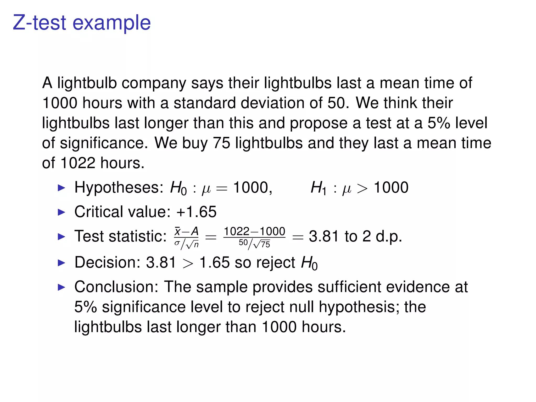
A lightbulb company says their lightbulbs last a mean time of
1000 hours with a standard deviation of 50. We think their
lightbulbs last longer than this and propose a test at a 5% level
of significance. We buy 75 lightbulbs and they last a mean time
of 1022 hours.
Hypotheses: H0 : µ = 1000, H1 : µ > 1000
Critical value: +1.65
Test statistic: ¯x−A
σ/
√
n
= 1022−1000
50/
√
75
= 3.81 to 2 d.p.
Decision: 3.81 > 1.65 so reject H0
Conclusion: The sample provides sufficient evidence at
5% significance level to reject null hypothesis; the
lightbulbs last longer than 1000 hours.

4. Z-test summary
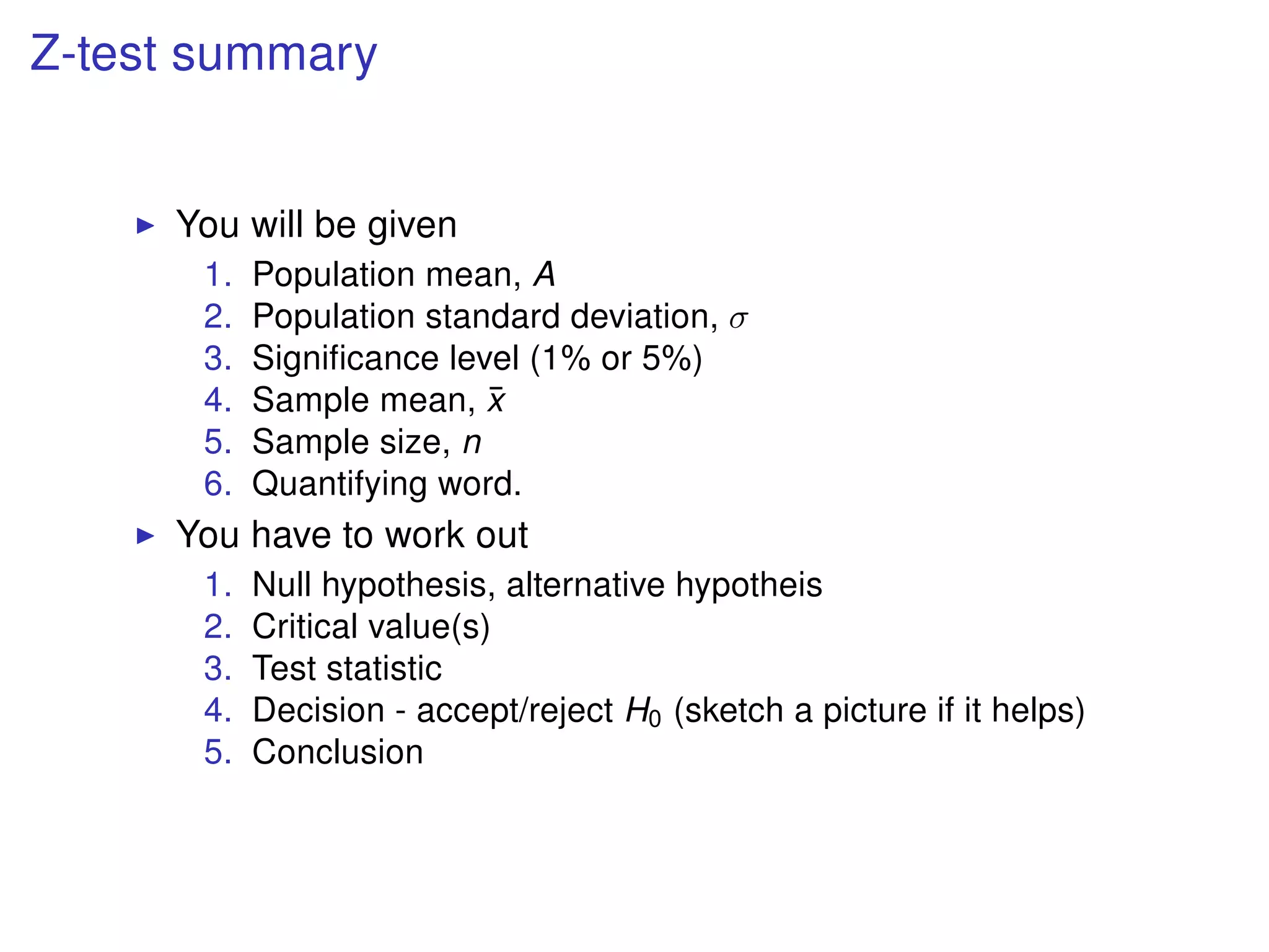
You will be given
1. Population mean, A
2. Population standard deviation, σ
3. Significance level (1% or 5%)
4. Sample mean, ¯x
5. Sample size, n
6. Quantifying word.
You have to work out
1. Null hypothesis, alternative hypotheis
2. Critical value(s)
3. Test statistic
4. Decision - accept/reject H0 (sketch a picture if it helps)
5. Conclusion

5. The difference between a Z-test and a T-test
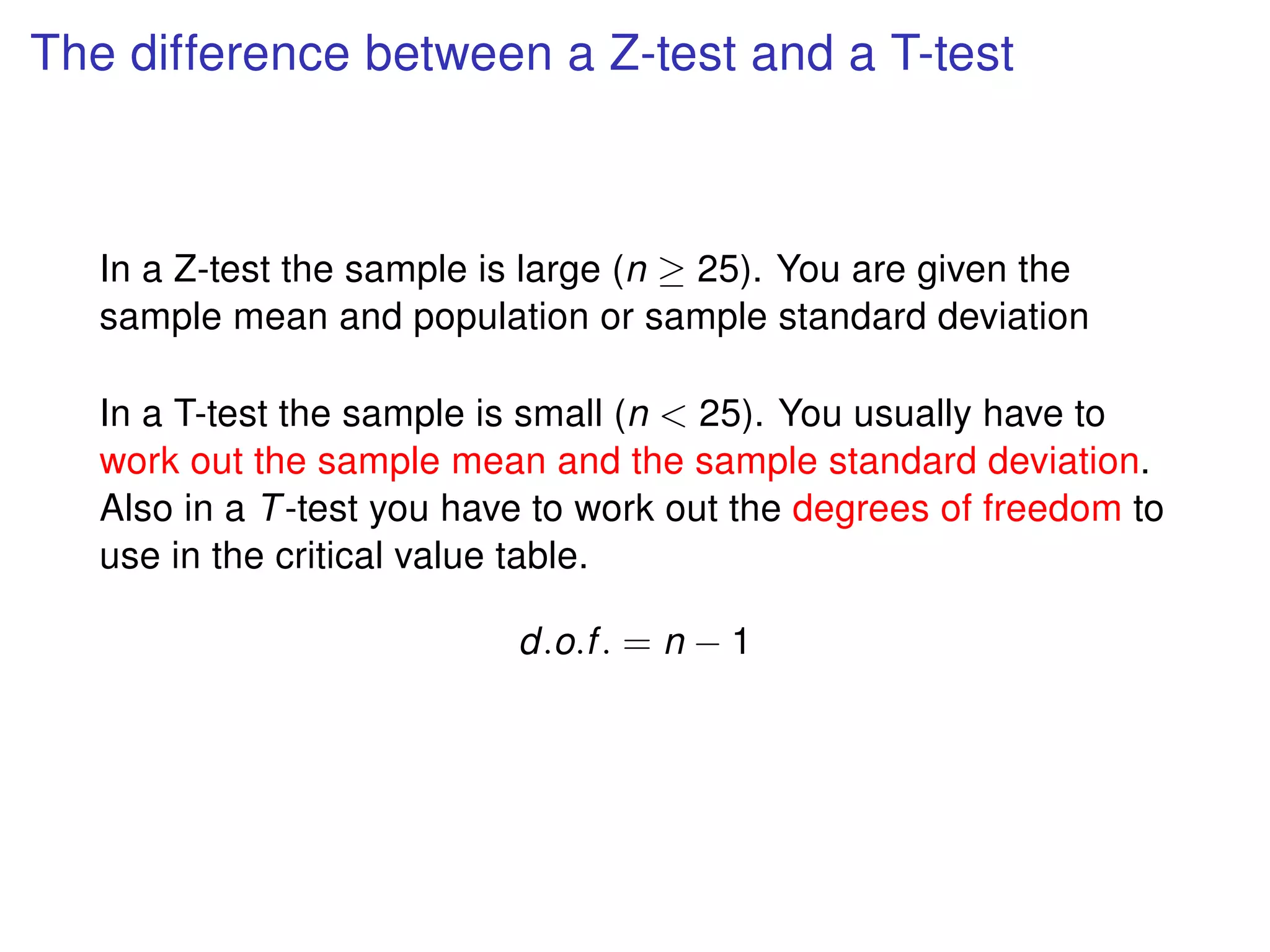
In a Z-test the sample is large (n ≥ 25). You are given the
sample mean and population or sample standard deviation
In a T-test the sample is small (n < 25). You usually have to
work out the sample mean and the sample standard deviation.
Also in a T-test you have to work out the degrees of freedom to
use in the critical value table.
d.o.f. = n − 1

6. T-test summary
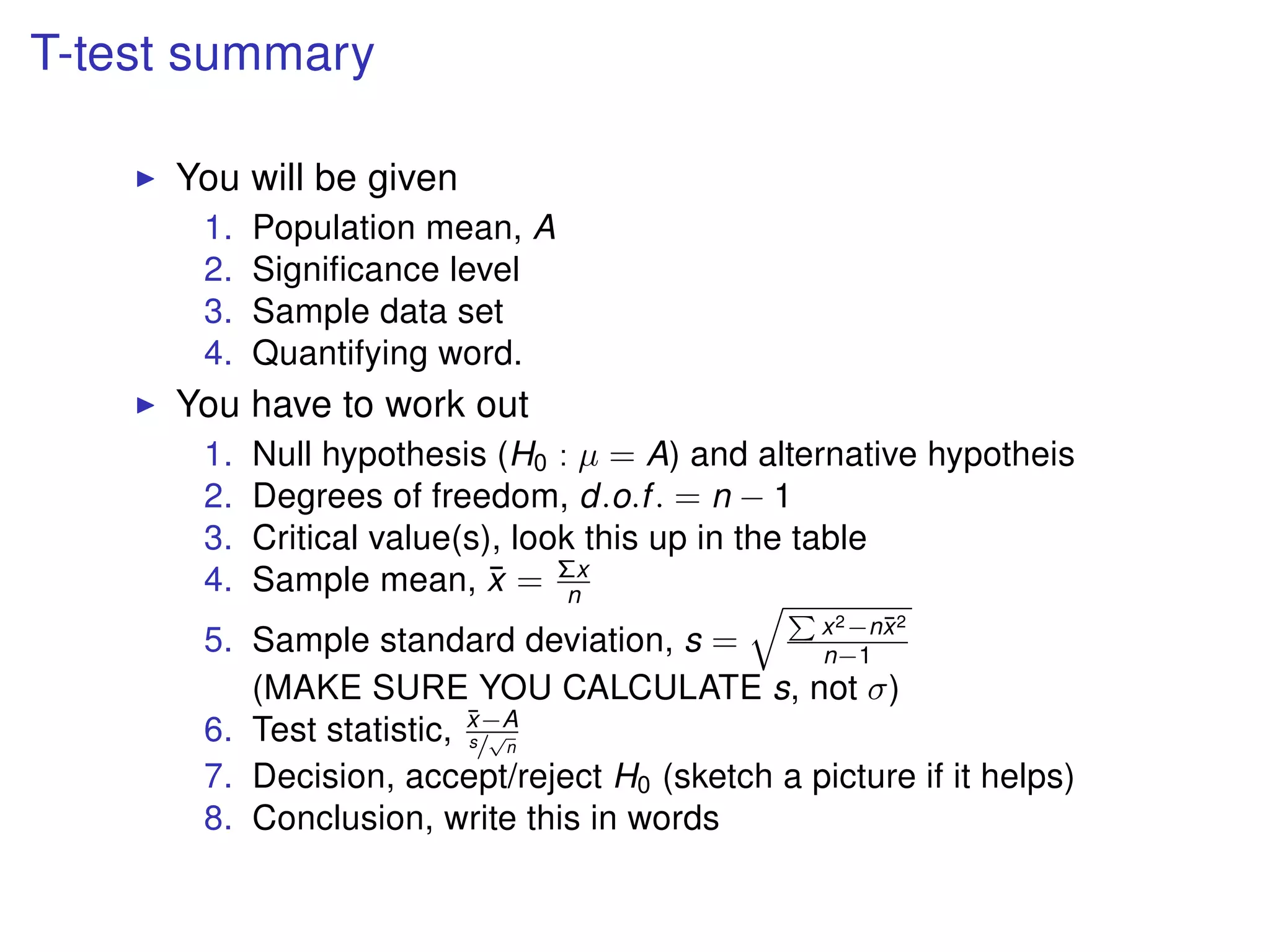
You will be given
1. Population mean, A
2. Significance level
3. Sample data set
4. Quantifying word.
You have to work out
1. Null hypothesis (H0 : µ = A) and alternative hypotheis
2. Degrees of freedom, d.o.f. = n − 1
3. Critical value(s), look this up in the table
4. Sample mean, ¯x = Σx
n
5. Sample standard deviation, s = x2−n¯x2
n−1
(MAKE SURE YOU CALCULATE s, not σ)
6. Test statistic, ¯x−A
s/
√
n
7. Decision, accept/reject H0 (sketch a picture if it helps)
8. Conclusion, write this in words

7. The null hypothesis and the alternative hypothesis for
the Z-test and T-test
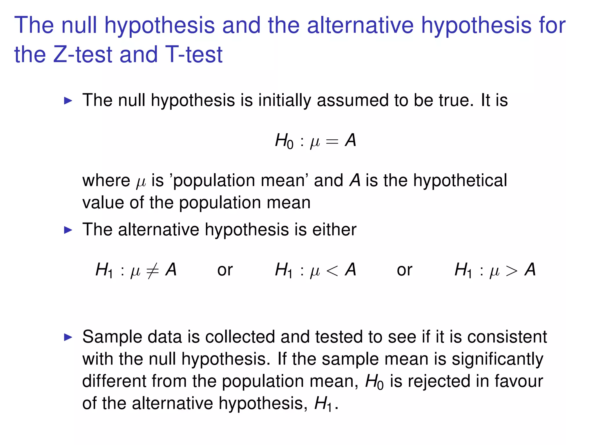
The null hypothesis is initially assumed to be true. It is
H0 : µ = A
where µ is ’population mean’ and A is the hypothetical
value of the population mean
The alternative hypothesis is either
H1 : µ = A or H1 : µ < A or H1 : µ > A
Sample data is collected and tested to see if it is consistent
with the null hypothesis. If the sample mean is significantly
different from the population mean, H0 is rejected in favour
of the alternative hypothesis, H1.

8. Significance level
The null hypothesis will always be tested to a given level of
significance.
A 5% level of significance means we are testing to see if
the probability of getting the sample mean is less than
0.05. If the probability is less we reject the null hypothesis
in favour of the alternative hypothesis.
A 1% level of significance translates to a probability of 0.01.

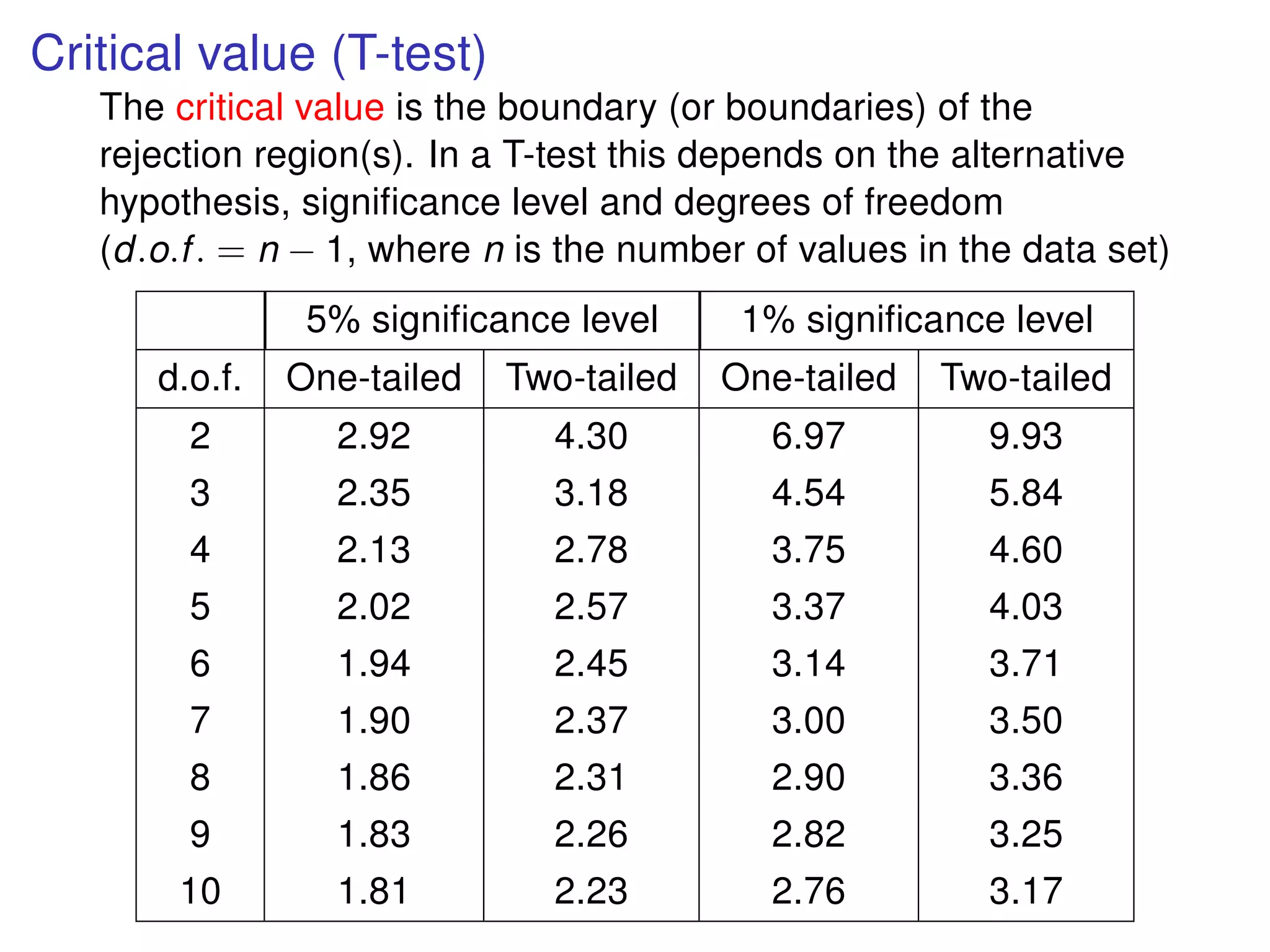
9. Critical value (T-test)
The critical value is the boundary (or boundaries) of the
rejection region(s). In a T-test this depends on the alternative
hypothesis, significance level and degrees of freedom
(d.o.f. = n − 1, where n is the number of values in the data set)
5% significance level 1% significance level
d.o.f. One-tailed Two-tailed One-tailed Two-tailed
2 2.92 4.30 6.97 9.93
3 2.35 3.18 4.54 5.84
4 2.13 2.78 3.75 4.60
5 2.02 2.57 3.37 4.03
6 1.94 2.45 3.14 3.71
7 1.90 2.37 3.00 3.50
8 1.86 2.31 2.90 3.36
9 1.83 2.26 2.82 3.25
10 1.81 2.23 2.76 3.17

10. Degrees of freedom (T-test)
The degrees of freedom of a set of data is a way of
measuring how the tests effect each other.
If the data has size n and each sample does not effect any
others the degree of freedom is n − 1. (This is usually the
case with our data).
Consider a bag containing 10 stones.
If as a sample we pick out 10 stones our degree of
freedom is 0 because the choice of the first one constrains
the possibilities for all others and the final one is left with
no choices.
If as a sample we pick out 7 stones our degree of freedom
is 3 because if we take out three stones before we start the
choice of stones is unique.
If as a sample we just pick out 1 stone our degree of
freedom is 9.

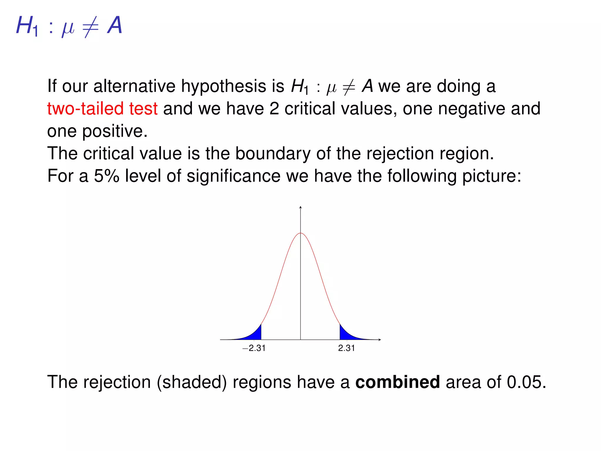
11. H1 : µ = A
If our alternative hypothesis is H1 : µ = A we are doing a
two-tailed test and we have 2 critical values, one negative and
one positive.
The critical value is the boundary of the rejection region.
For a 5% level of significance we have the following picture:
−2.31 2.31
The rejection (shaded) regions have a combined area of 0.05.

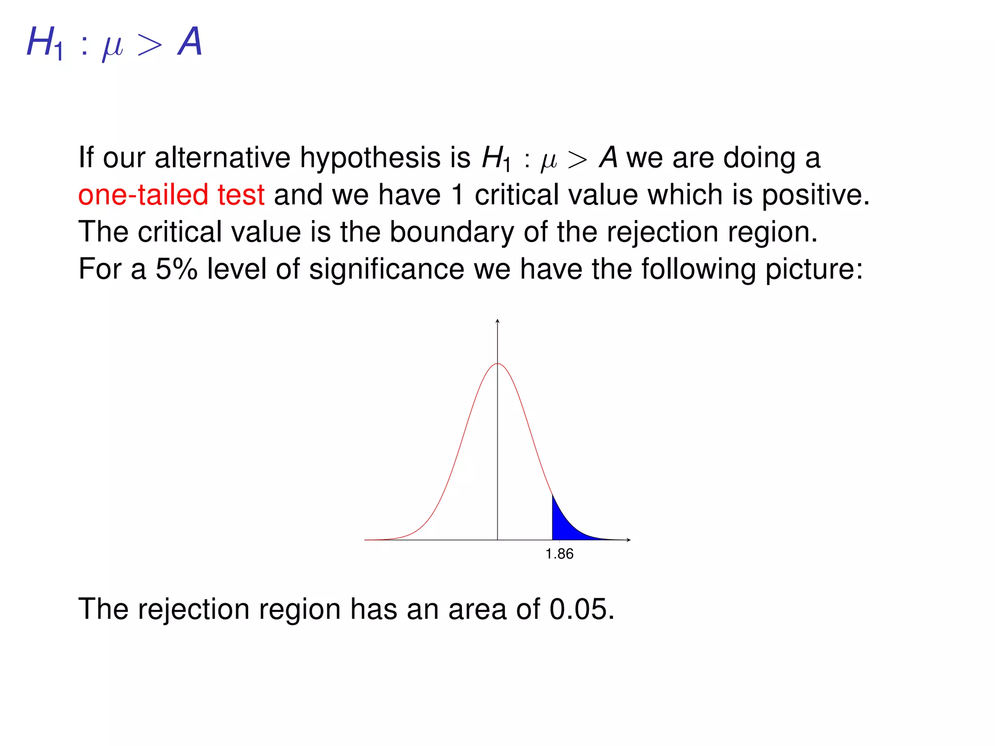
12. H1 : µ > A
If our alternative hypothesis is H1 : µ > A we are doing a
one-tailed test and we have 1 critical value which is positive.
The critical value is the boundary of the rejection region.
For a 5% level of significance we have the following picture:
1.86
The rejection region has an area of 0.05.

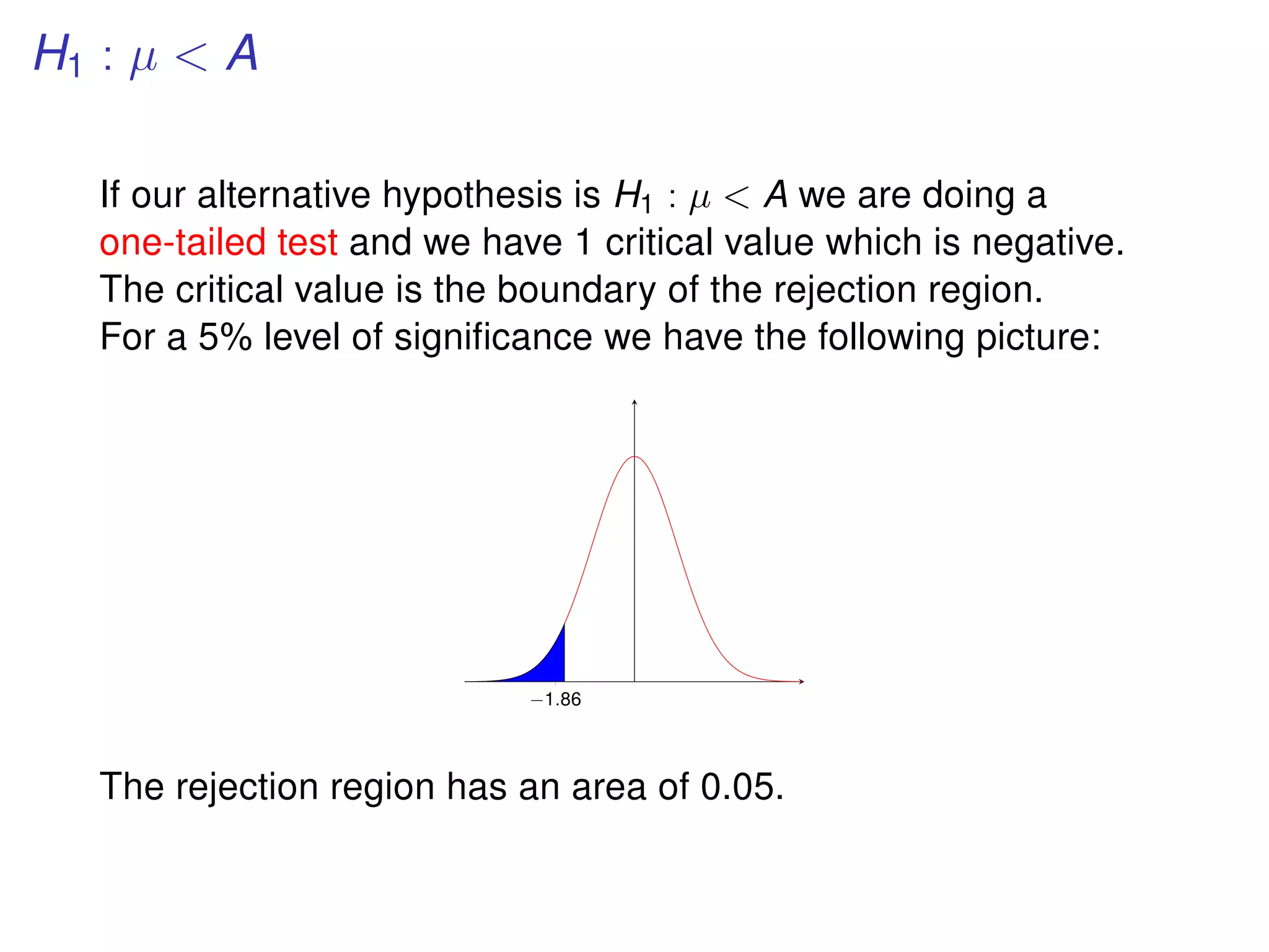
13. H1 : µ < A
If our alternative hypothesis is H1 : µ < A we are doing a
one-tailed test and we have 1 critical value which is negative.
The critical value is the boundary of the rejection region.
For a 5% level of significance we have the following picture:
−1.86
The rejection region has an area of 0.05.

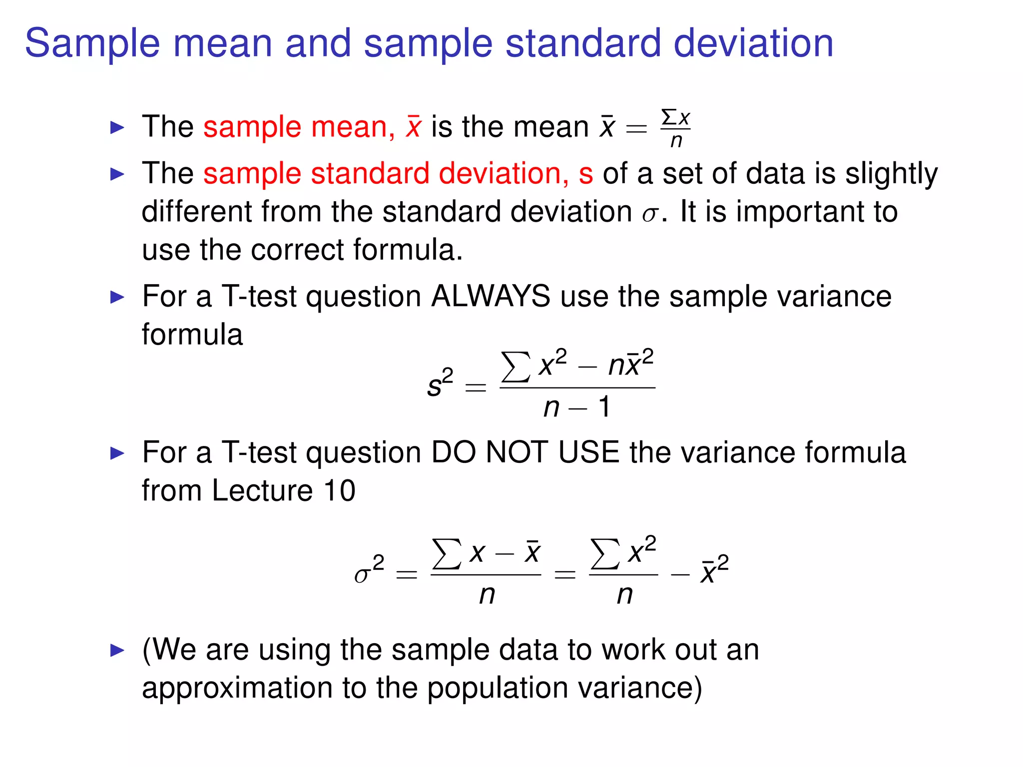
14. Sample mean and sample standard deviation
The sample mean, ¯x is the mean ¯x = Σx
n
The sample standard deviation, s of a set of data is slightly
different from the standard deviation σ. It is important to
use the correct formula.
For a T-test question ALWAYS use the sample variance
formula
s2
=
x2 − n¯x2
n − 1
For a T-test question DO NOT USE the variance formula
from Lecture 10
σ2
=
x − ¯x
n
=
x2
n
− ¯x2
(We are using the sample data to work out an
approximation to the population variance)

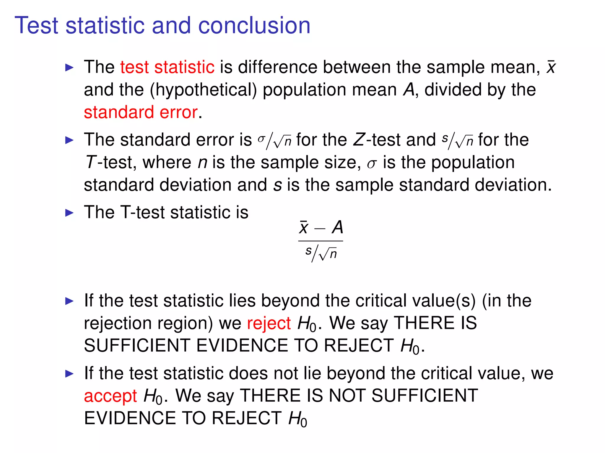
15. Test statistic and conclusion
The test statistic is difference between the sample mean, ¯x
and the (hypothetical) population mean A, divided by the
standard error.
The standard error is σ/
√
n for the Z-test and s/
√
n for the
T-test, where n is the sample size, σ is the population
standard deviation and s is the sample standard deviation.
The T-test statistic is
¯x − A
s/
√
n
If the test statistic lies beyond the critical value(s) (in the
rejection region) we reject H0. We say THERE IS
SUFFICIENT EVIDENCE TO REJECT H0.
If the test statistic does not lie beyond the critical value, we
accept H0. We say THERE IS NOT SUFFICIENT
EVIDENCE TO REJECT H0

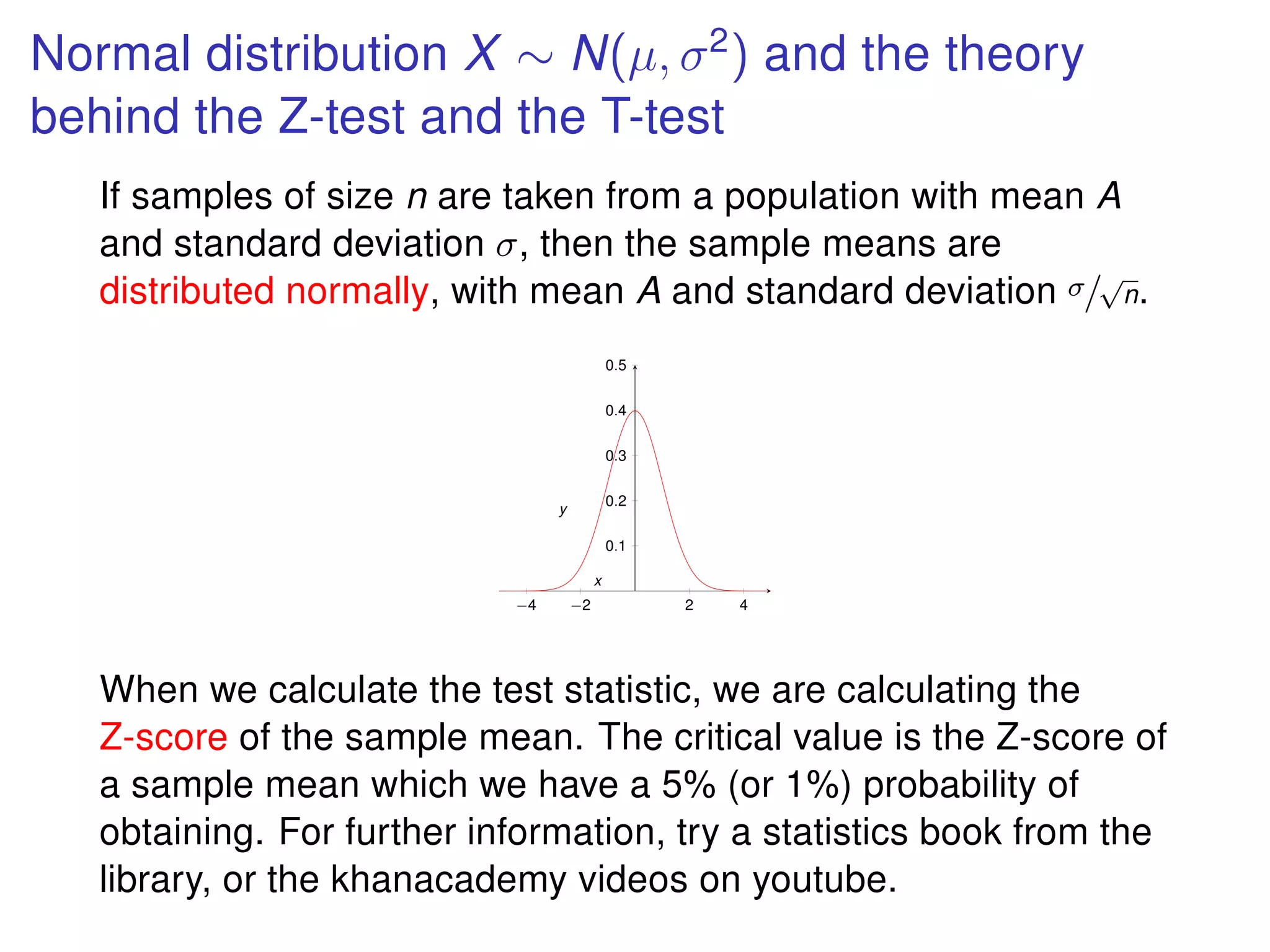
16. Normal distribution X ∼ N(µ, σ2
) and the theory
behind the Z-test and the T-test
If samples of size n are taken from a population with mean A
and standard deviation σ, then the sample means are
distributed normally, with mean A and standard deviation σ/
√
n.
−4 −2 2 4
0.1
0.2
0.3
0.4
0.5
x
y
When we calculate the test statistic, we are calculating the
Z-score of the sample mean. The critical value is the Z-score of
a sample mean which we have a 5% (or 1%) probability of
obtaining. For further information, try a statistics book from the
library, or the khanacademy videos on youtube.

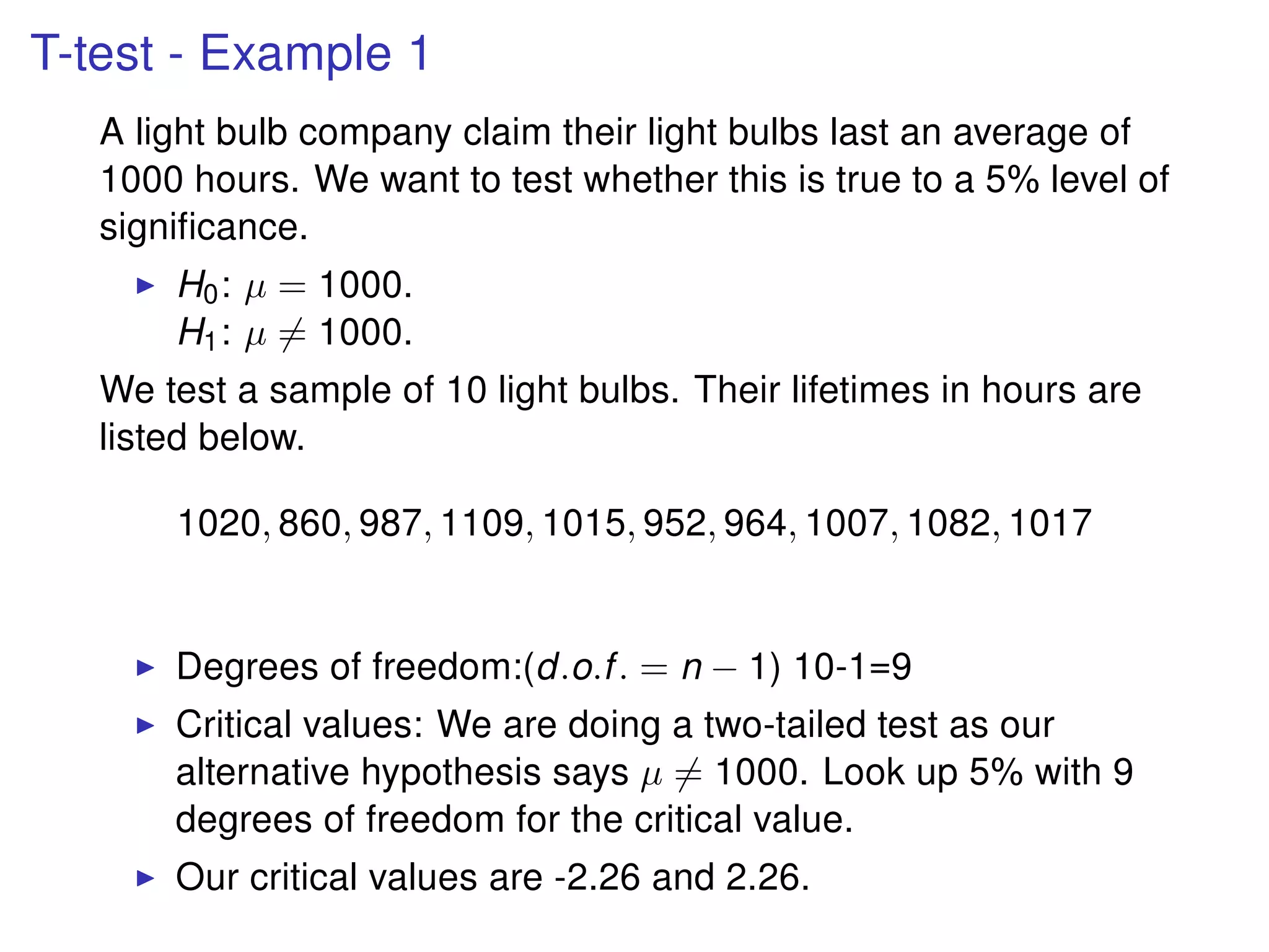
17. T-test - Example 1
A light bulb company claim their light bulbs last an average of
1000 hours. We want to test whether this is true to a 5% level of
significance.
H0: µ = 1000.
H1: µ = 1000.
We test a sample of 10 light bulbs. Their lifetimes in hours are
listed below.
1020, 860, 987, 1109, 1015, 952, 964, 1007, 1082, 1017
Degrees of freedom:(d.o.f. = n − 1) 10-1=9
Critical values: We are doing a two-tailed test as our
alternative hypothesis says µ = 1000. Look up 5% with 9
degrees of freedom for the critical value.
Our critical values are -2.26 and 2.26.

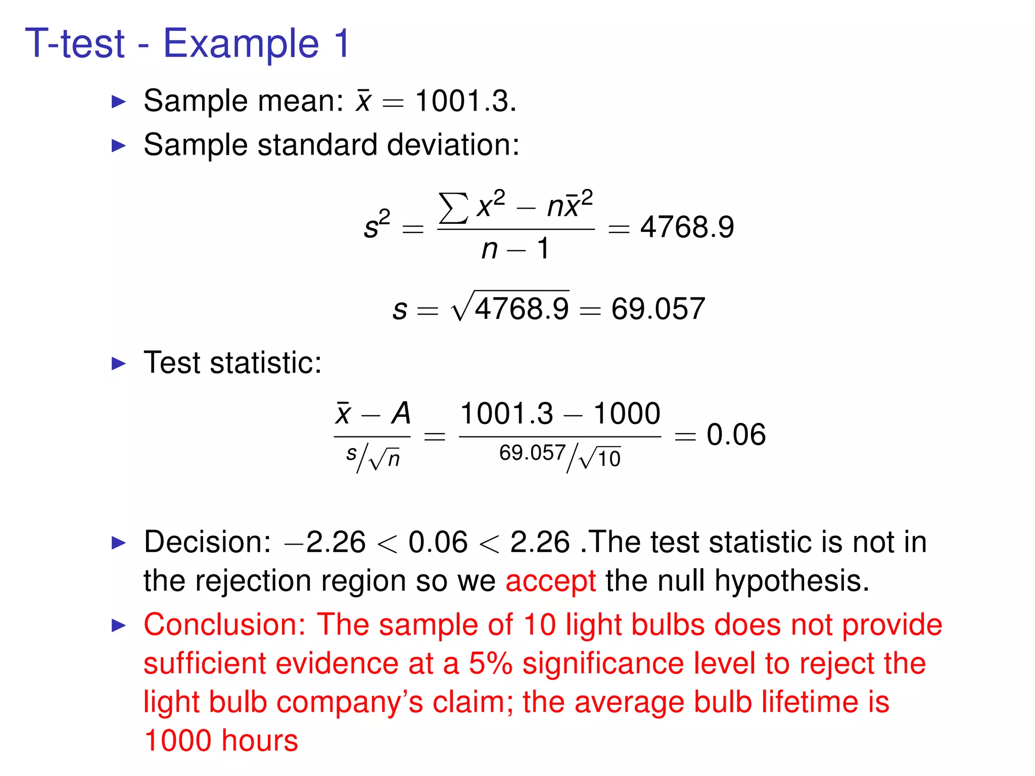
18. T-test - Example 1
Sample mean: ¯x = 1001.3.
Sample standard deviation:
s2
=
x2 − n¯x2
n − 1
= 4768.9
s =
√
4768.9 = 69.057
Test statistic:
¯x − A
s/
√
n
=
1001.3 − 1000
69.057/
√
10
= 0.06
Decision: −2.26 < 0.06 < 2.26 .The test statistic is not in
the rejection region so we accept the null hypothesis.
Conclusion: The sample of 10 light bulbs does not provide
sufficient evidence at a 5% significance level to reject the
light bulb company’s claim; the average bulb lifetime is
1000 hours

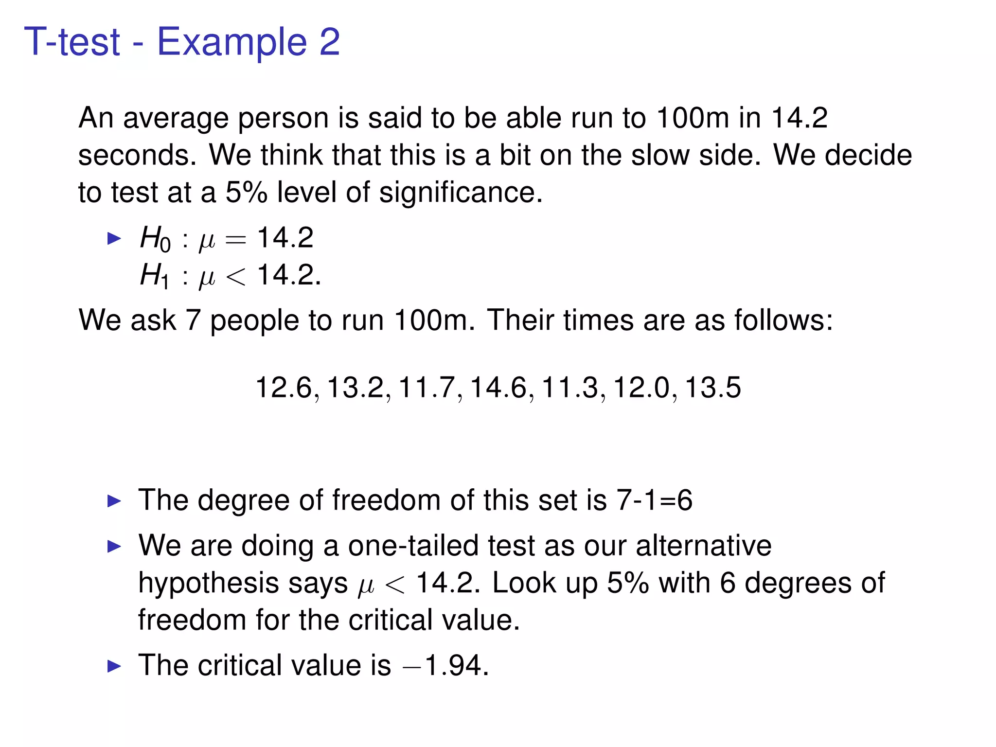
19. T-test - Example 2
An average person is said to be able run to 100m in 14.2
seconds. We think that this is a bit on the slow side. We decide
to test at a 5% level of significance.
H0 : µ = 14.2
H1 : µ < 14.2.
We ask 7 people to run 100m. Their times are as follows:
12.6, 13.2, 11.7, 14.6, 11.3, 12.0, 13.5
The degree of freedom of this set is 7-1=6
We are doing a one-tailed test as our alternative
hypothesis says µ < 14.2. Look up 5% with 6 degrees of
freedom for the critical value.
The critical value is −1.94.

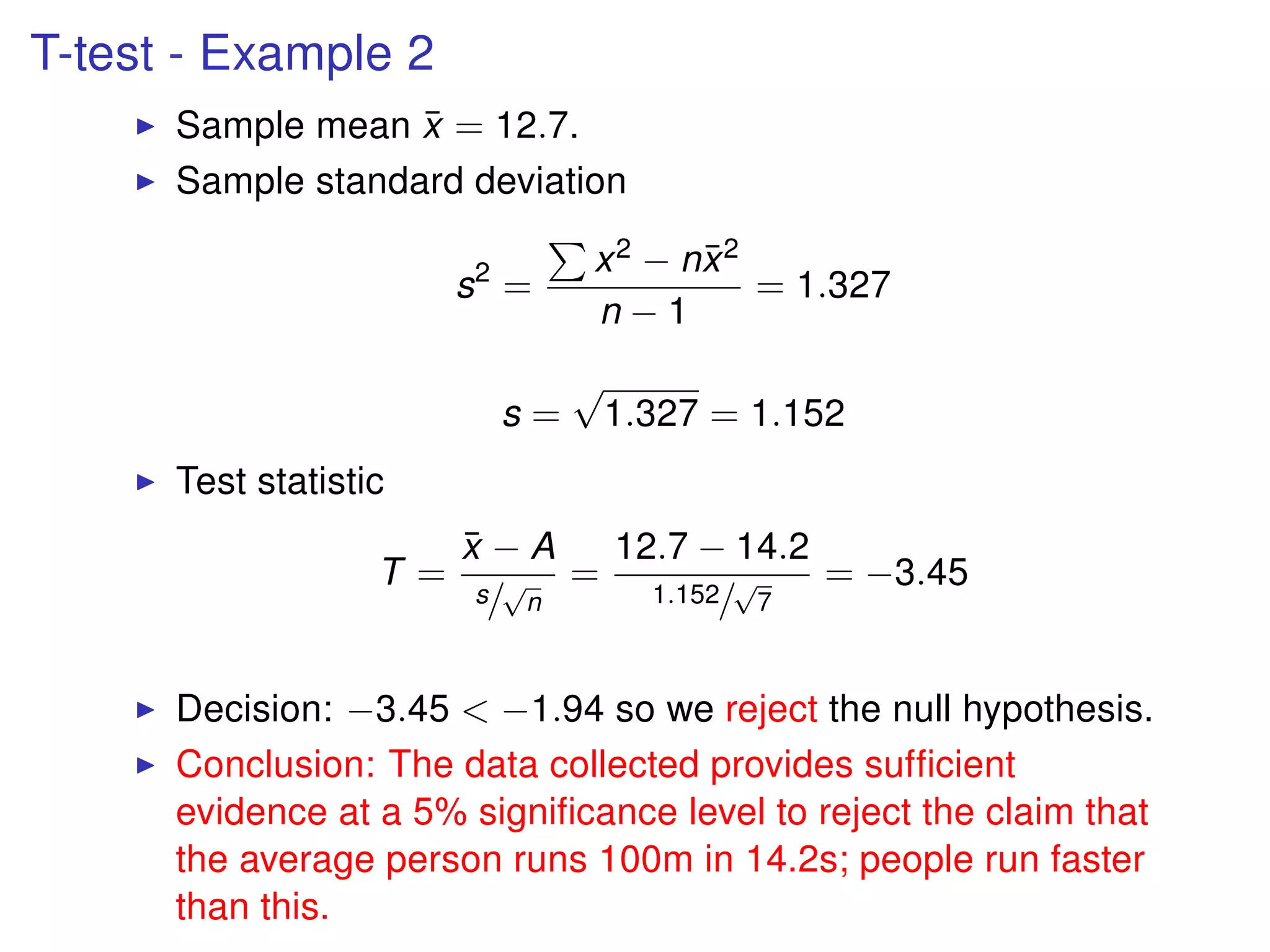
20. T-test - Example 2
Sample mean ¯x = 12.7.
Sample standard deviation
s2
=
x2 − n¯x2
n − 1
= 1.327
s =
√
1.327 = 1.152
Test statistic
T =
¯x − A
s/
√
n
=
12.7 − 14.2
1.152/
√
7
= −3.45
Decision: −3.45 < −1.94 so we reject the null hypothesis.
Conclusion: The data collected provides sufficient
evidence at a 5% significance level to reject the claim that
the average person runs 100m in 14.2s; people run faster
than this.

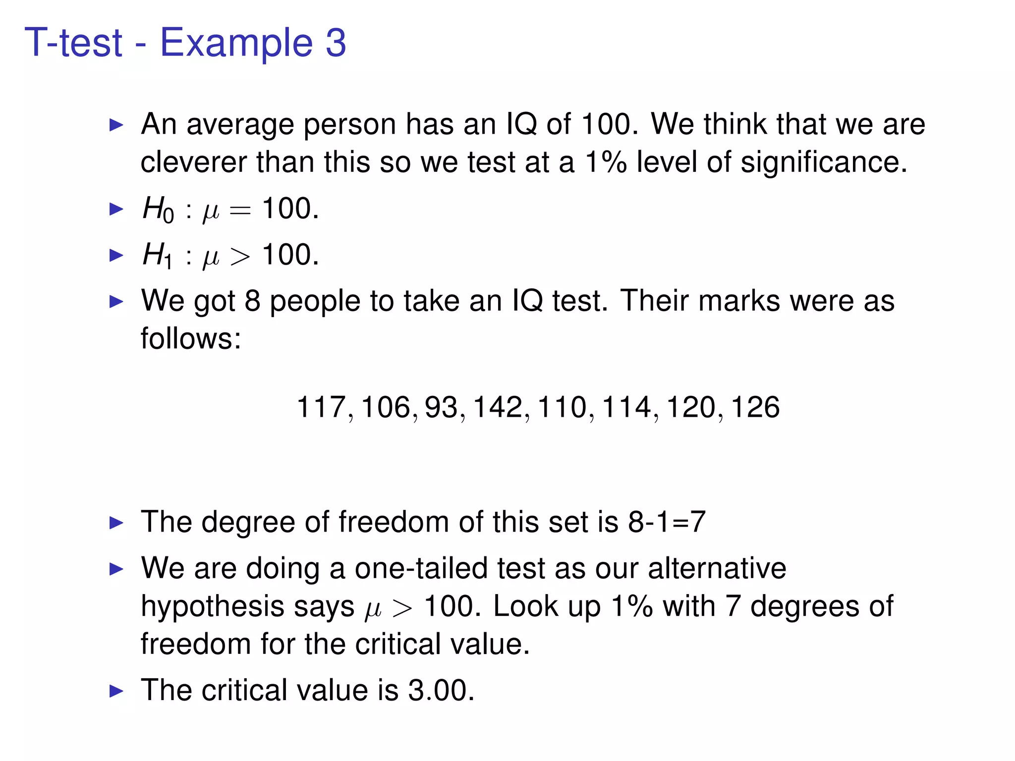
21. T-test - Example 3
An average person has an IQ of 100. We think that we are
cleverer than this so we test at a 1% level of significance.
H0 : µ = 100.
H1 : µ > 100.
We got 8 people to take an IQ test. Their marks were as
follows:
117, 106, 93, 142, 110, 114, 120, 126
The degree of freedom of this set is 8-1=7
We are doing a one-tailed test as our alternative
hypothesis says µ > 100. Look up 1% with 7 degrees of
freedom for the critical value.
The critical value is 3.00.

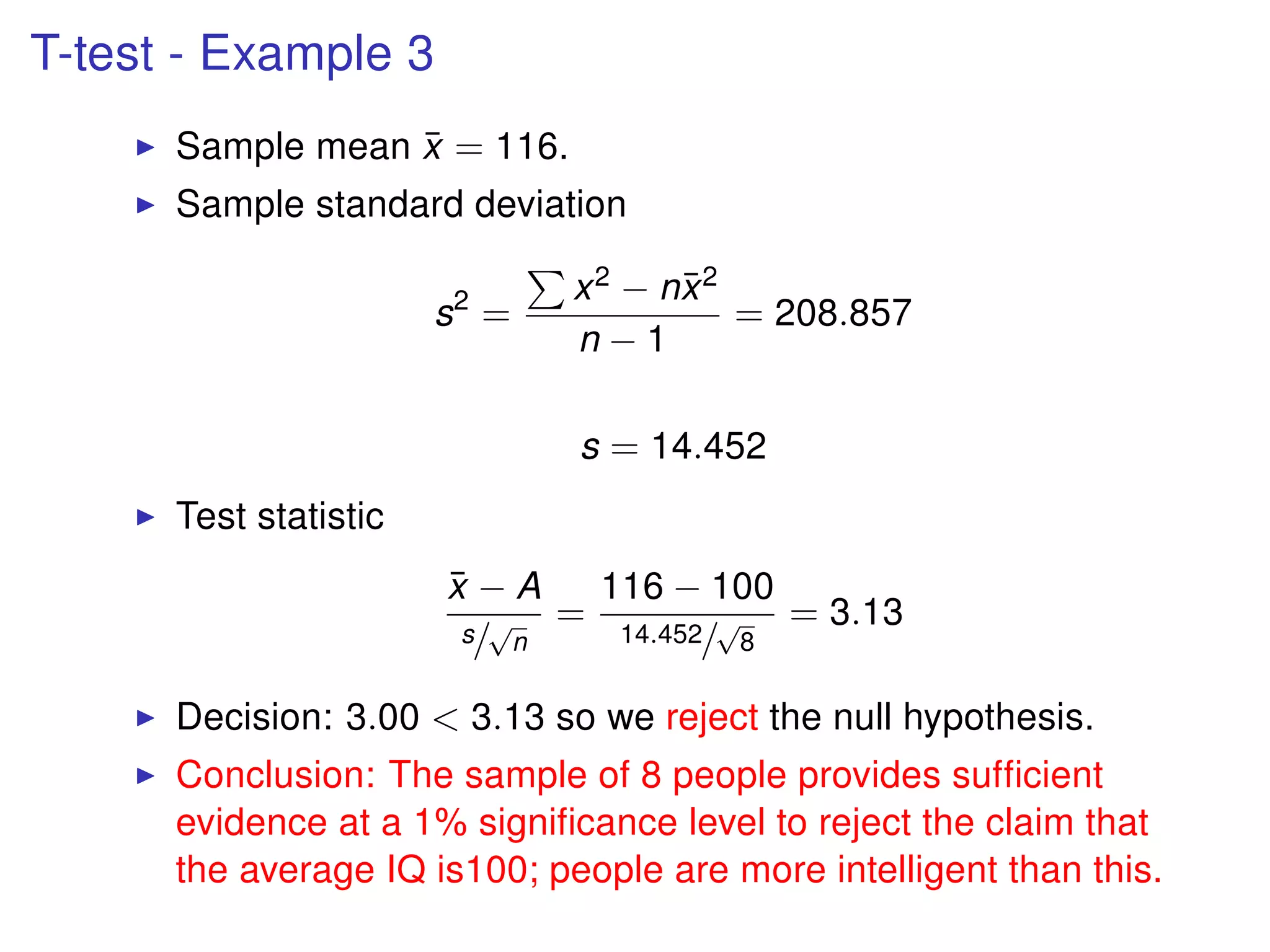
22. T-test - Example 3
Sample mean ¯x = 116.
Sample standard deviation
s2
=
x2 − n¯x2
n − 1
= 208.857
s = 14.452
Test statistic
¯x − A
s/
√
n
=
116 − 100
14.452/
√
8
= 3.13
Decision: 3.00 < 3.13 so we reject the null hypothesis.
Conclusion: The sample of 8 people provides sufficient
evidence at a 1% significance level to reject the claim that
the average IQ is100; people are more intelligent than this.

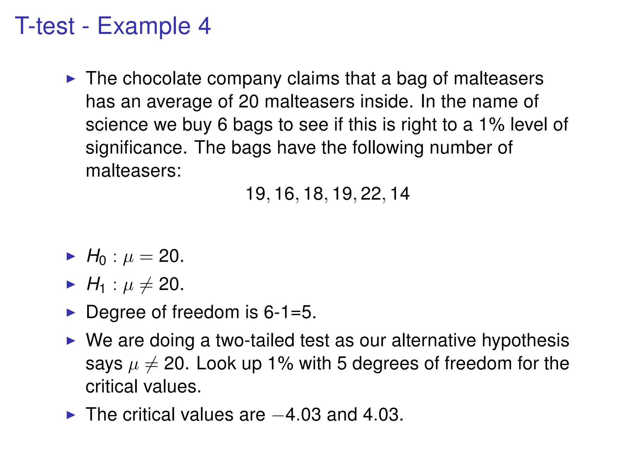
23. T-test - Example 4
The chocolate company claims that a bag of malteasers
has an average of 20 malteasers inside. In the name of
science we buy 6 bags to see if this is right to a 1% level of
significance. The bags have the following number of
malteasers:
19, 16, 18, 19, 22, 14
H0 : µ = 20.
H1 : µ = 20.
Degree of freedom is 6-1=5.
We are doing a two-tailed test as our alternative hypothesis
says µ = 20. Look up 1% with 5 degrees of freedom for the
critical values.
The critical values are −4.03 and 4.03.

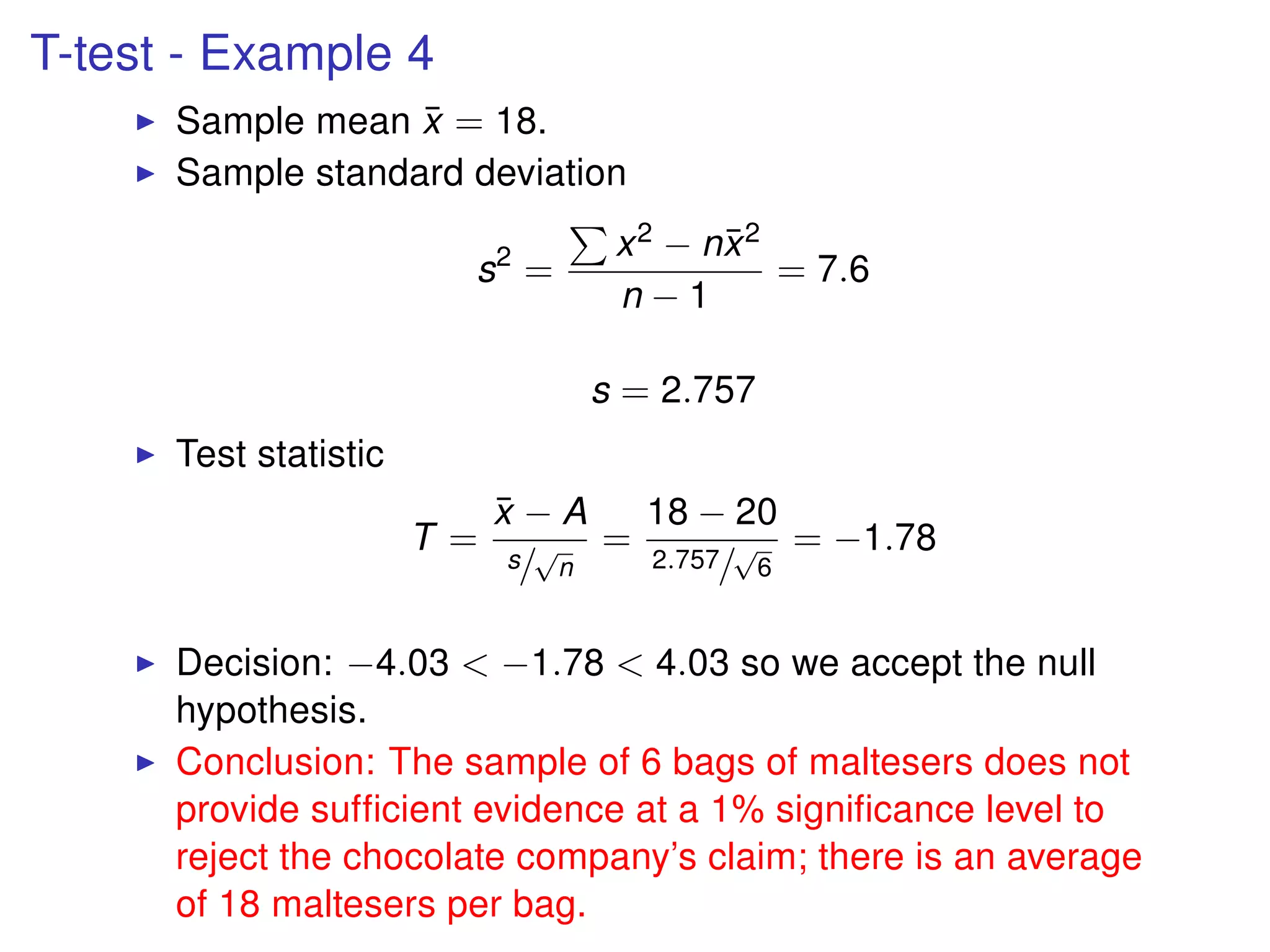
24. T-test - Example 4
Sample mean ¯x = 18.
Sample standard deviation
s2
=
x2 − n¯x2
n − 1
= 7.6
s = 2.757
Test statistic
T =
¯x − A
s/
√
n
=
18 − 20
2.757/
√
6
= −1.78
Decision: −4.03 < −1.78 < 4.03 so we accept the null
hypothesis.
Conclusion: The sample of 6 bags of maltesers does not
provide sufficient evidence at a 1% significance level to
reject the chocolate company’s claim; there is an average
of 18 maltesers per bag.