This document provides an overview of Load and Resistance Factor Design (LRFD) for deep foundations, with a focus on:
1. The differences between Allowable Stress Design (ASD) and LRFD approaches.
2. Key concepts in LRFD including limit states, load factors, load combinations, resistance factors, reliability, and efficiency of design methods.
3. How LRFD approaches are applied specifically to deep foundation design, including the use of limit states for service, strength, and extreme load conditions according to the AASHTO Bridge Design Specifications.
In this document
Powered by AI
Introduction to Load and Resistance Factor Design (LRFD) focused on deep foundations with presentation goals.
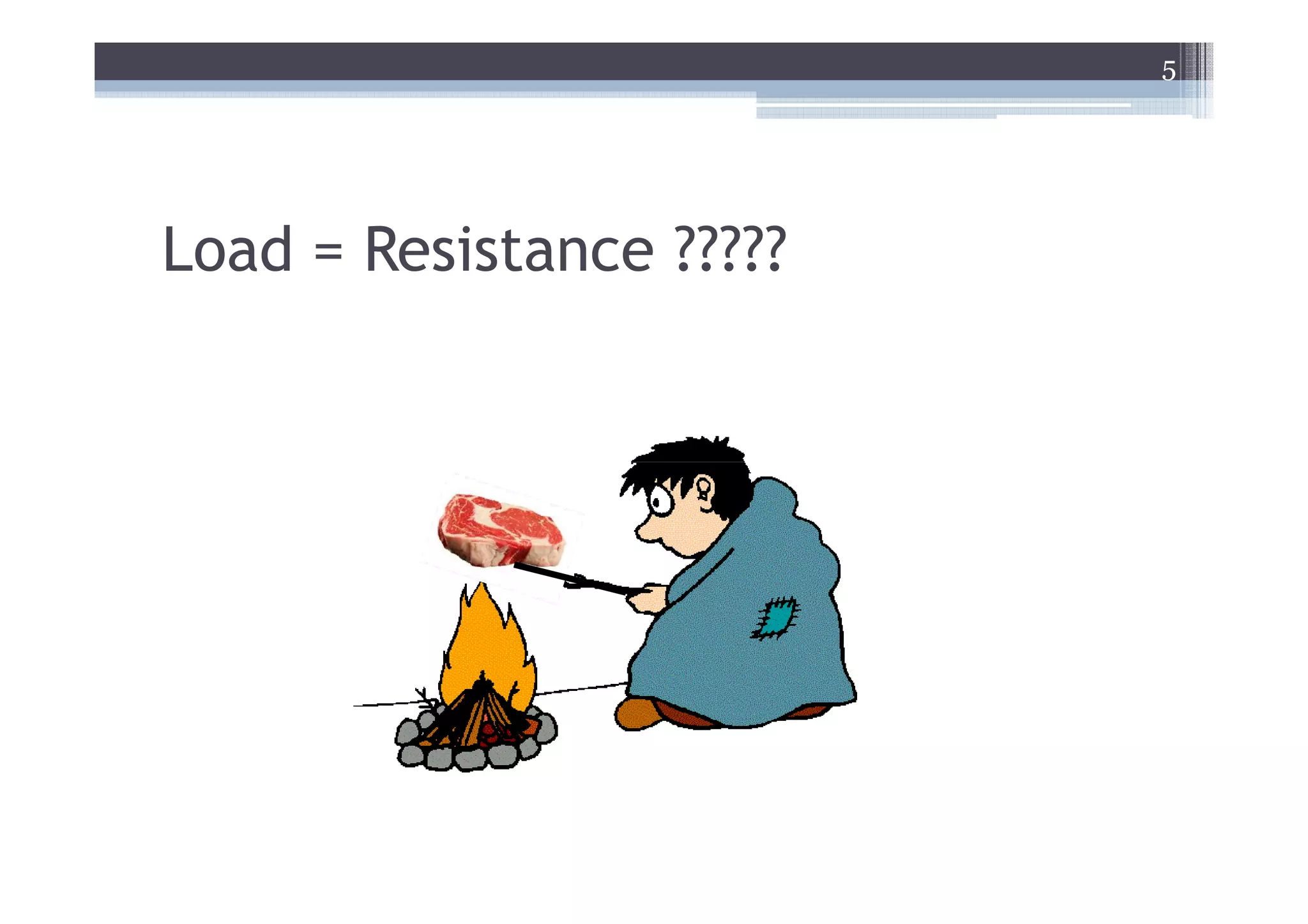
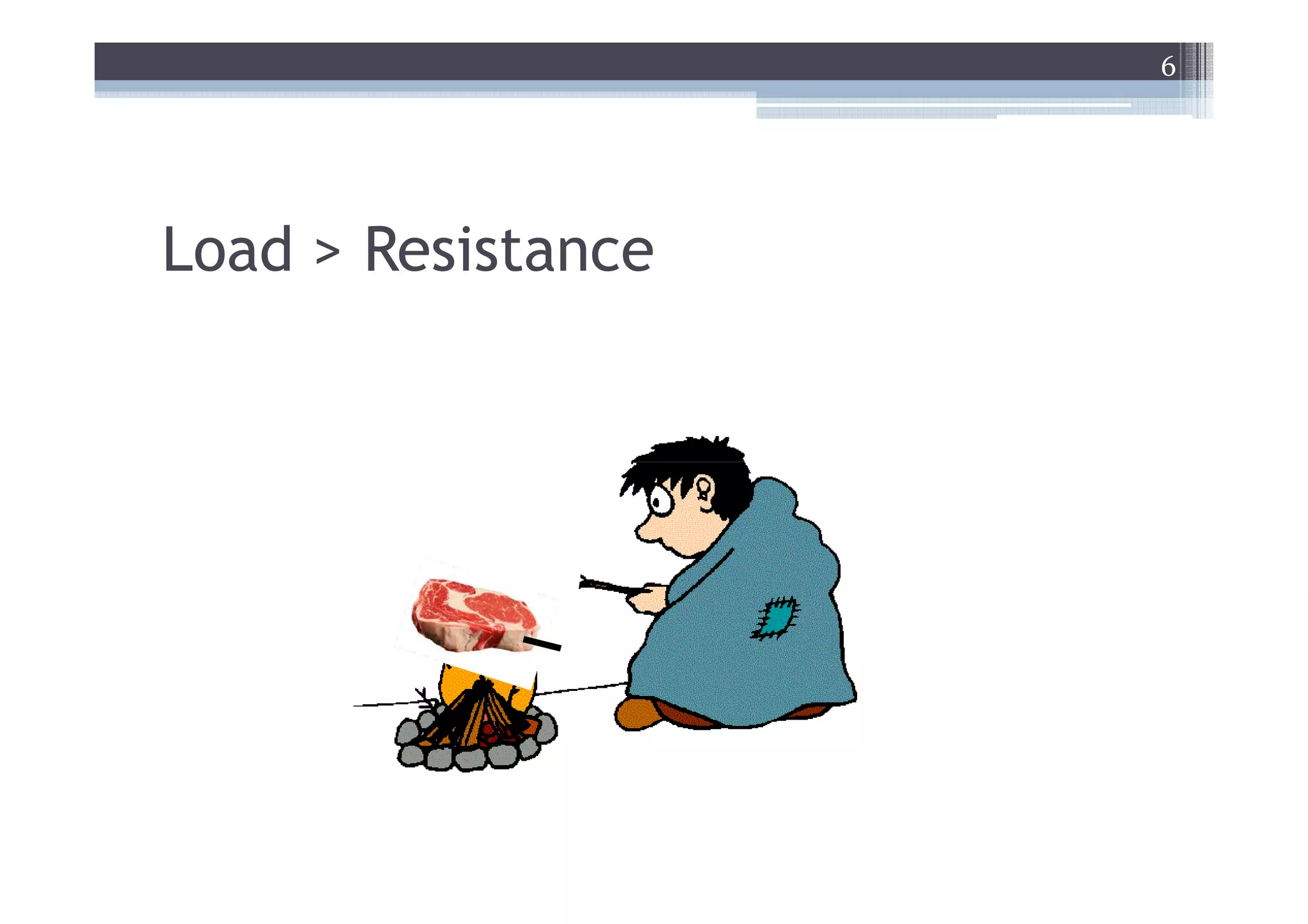
Understanding the conditions of load relative to resistance: Load < Resistance, Load = Resistance, Load > Resistance.
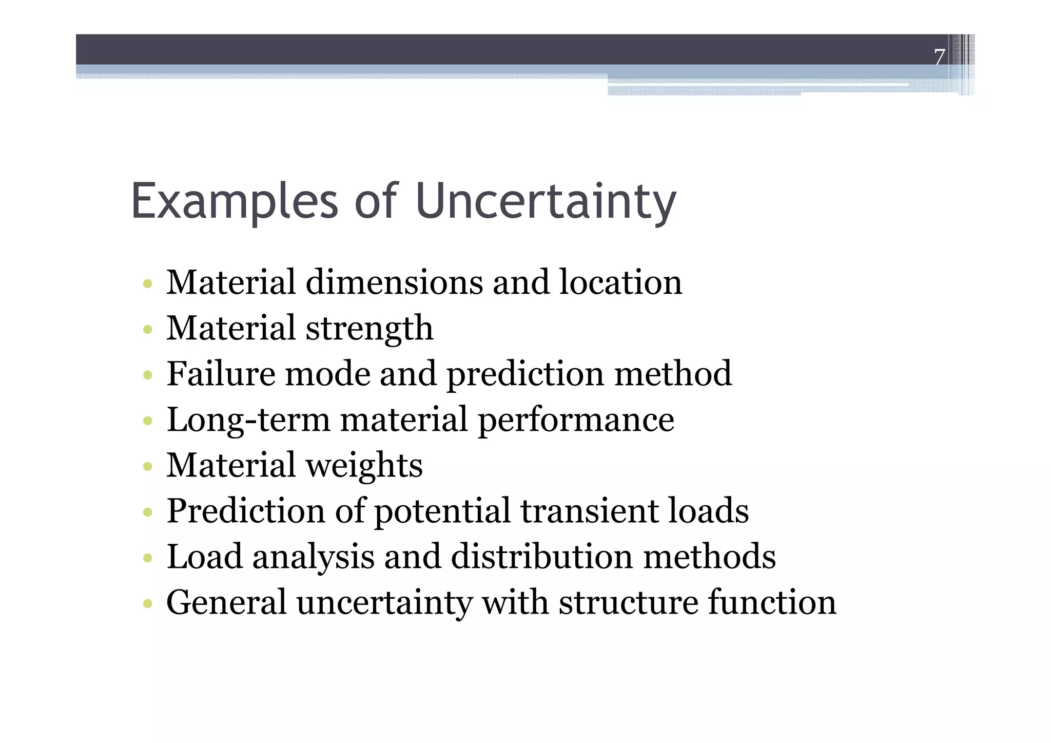
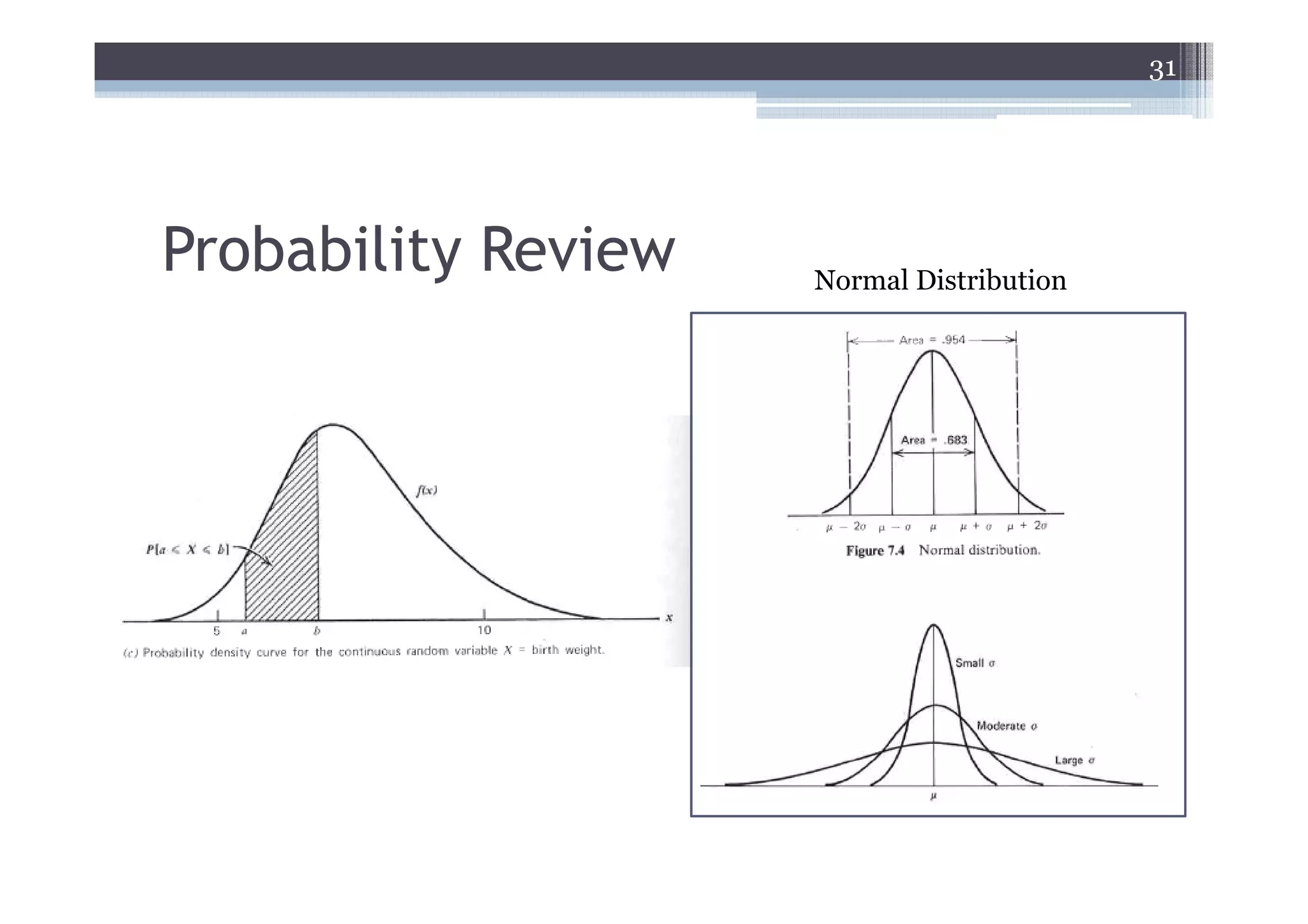
Discusses various uncertainties in structural design including material characteristics and load analysis.
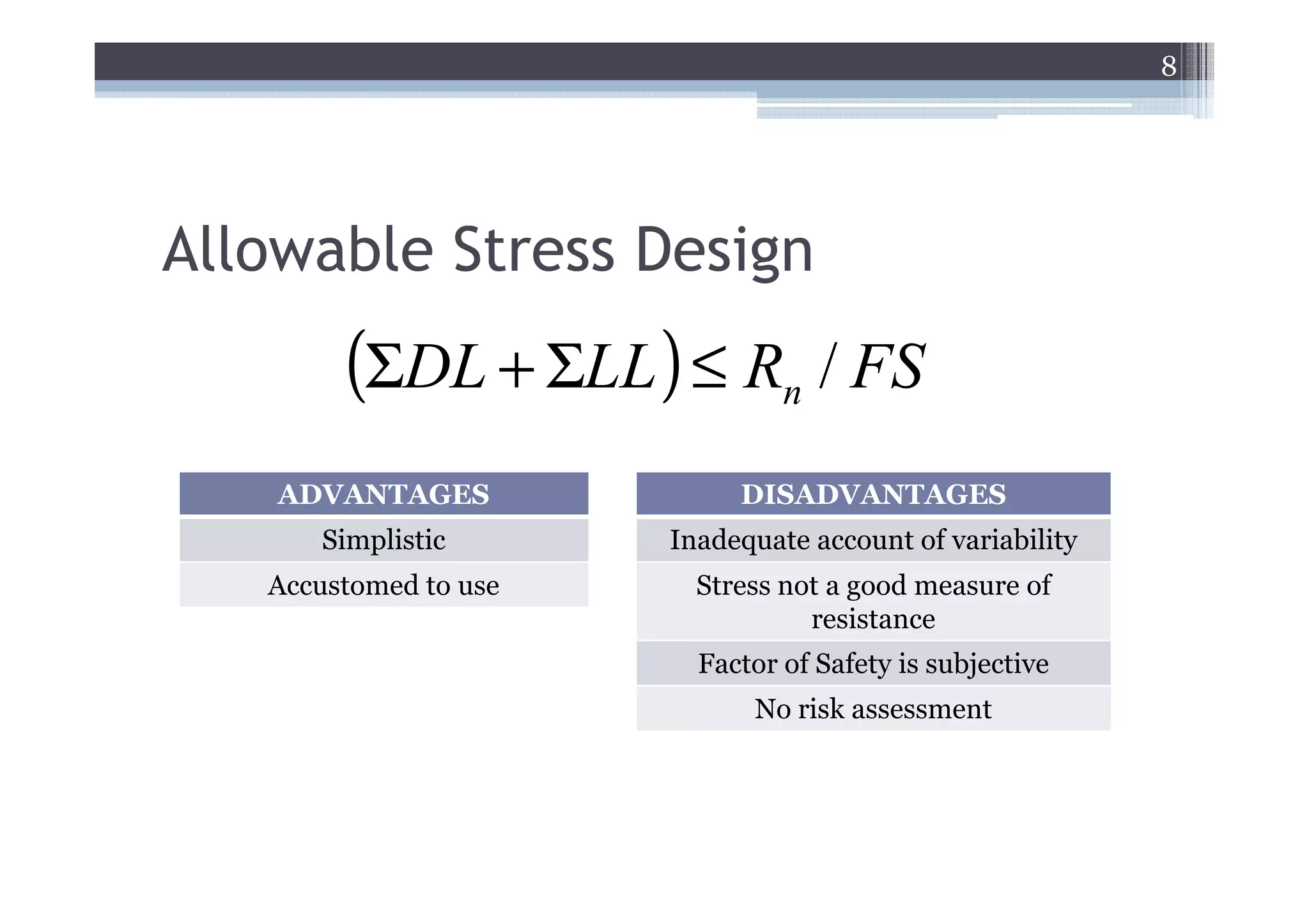
Analyzes Allowable Stress Design (ASD) and LRFD, indicating advantages and disadvantages of each method.
Describes LRFD equations, load factors, resistance factors, and limit states critical in deep foundations.
Understanding resistance factors and efficiency evaluations for reliable structural design outcomes.
Applies limit states methodology specifically regarding deep foundations and its construction implications.
Evaluates strength limit states for driven piles, drilled shafts, and micropiles within structural load bearing.
Explains both structural resistance values and driving resistance measures necessary for pile installations.
Addresses settlement calculations, assumptions made, and factors affecting the structural integrity of piles.
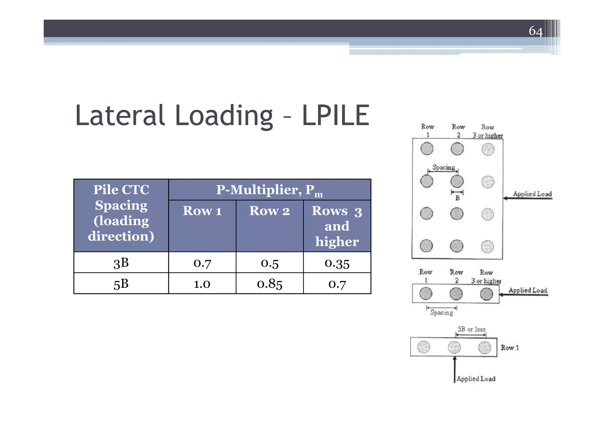
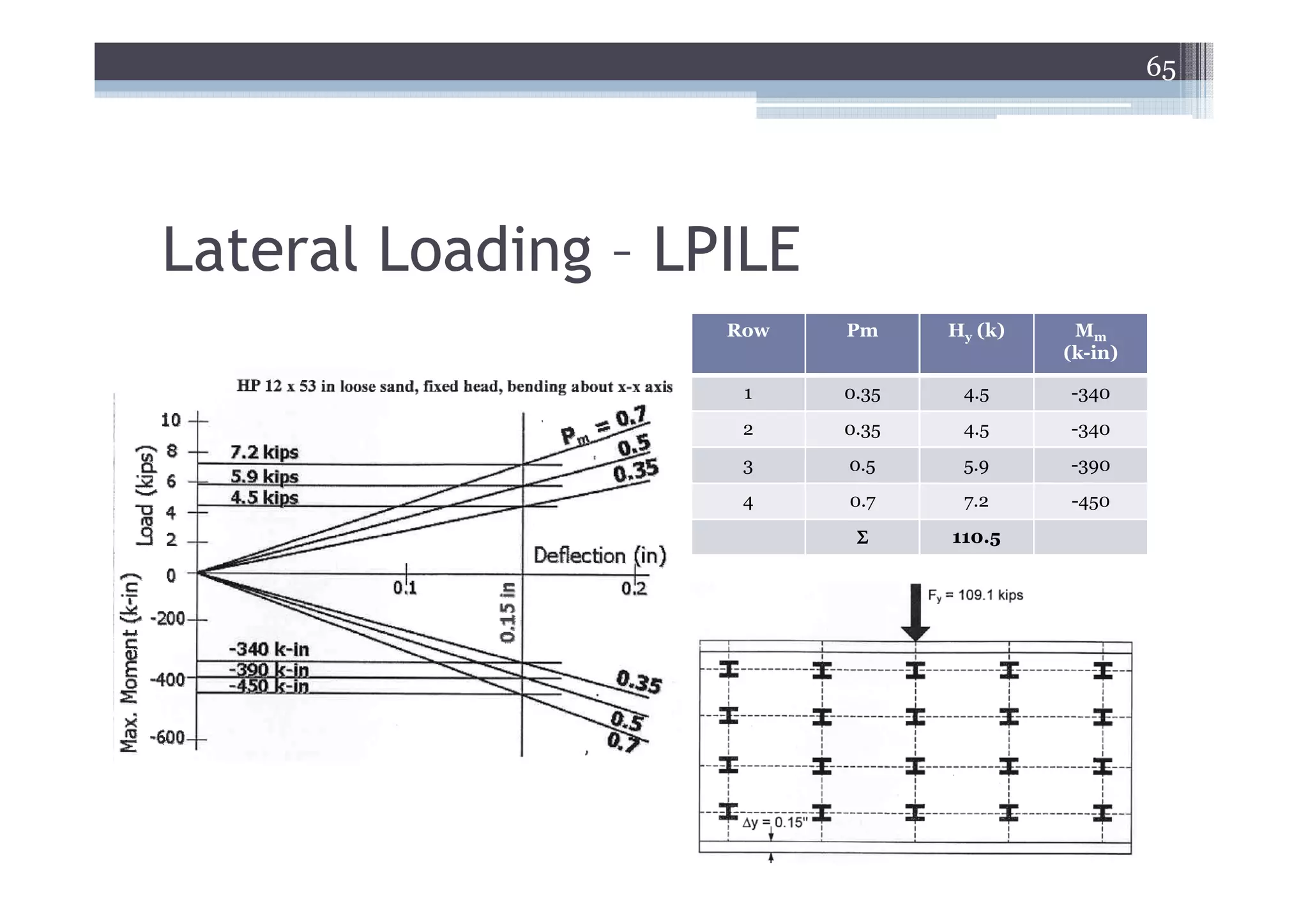
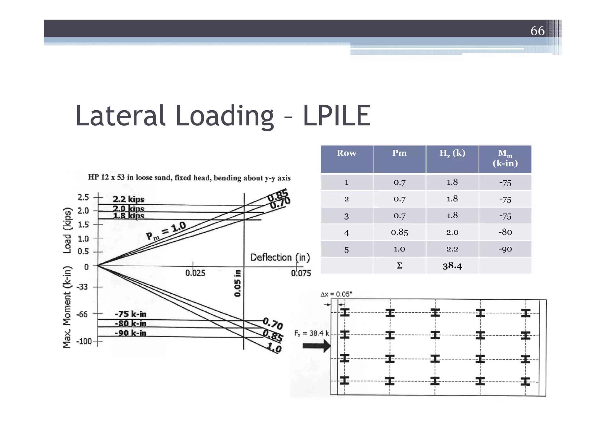
Discusses lateral loading effects on piles using specific calculations to ensure safety and stability.
Evaluates standard load combinations and performances for ensuring compliance with design specifications.
Specific case study examples detailing drilled shafts, resistance values and settlement analysis in practice.
1
Load and ResistanceFactor
Design (LRFD)- Deep Foundations
Donald C. Wotring, Ph.D., P.E.
February 2009
2.
2
Presentation
• This presentationis intended as a detailed
internal short-course with design examples. It
will also be used as a brown-bag lunch
presentation, but with less detail covered.
3.
3
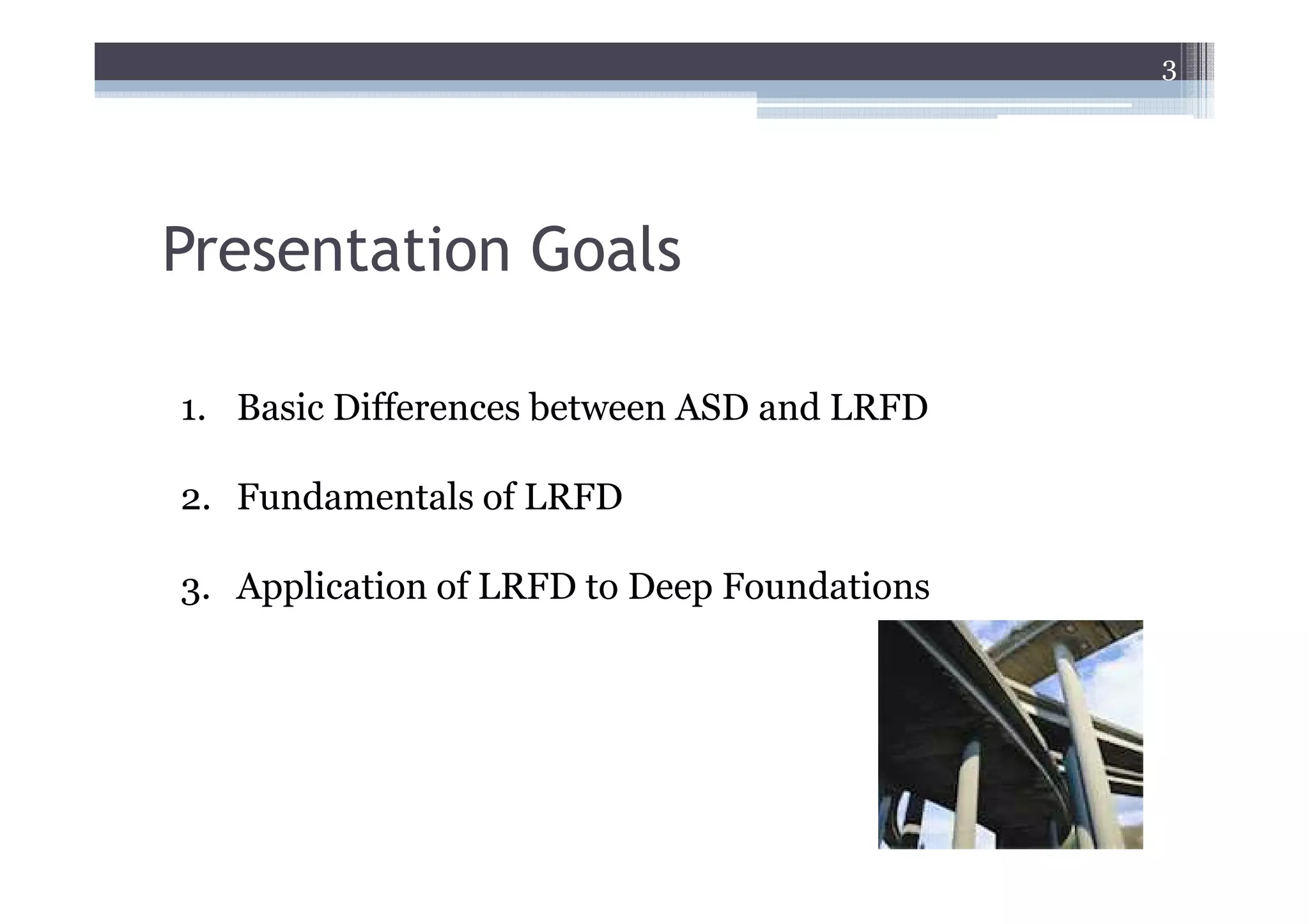
Presentation Goals
1. BasicDifferences between ASD and LRFD
2. Fundamentals of LRFD
3. Application of LRFD to Deep Foundations
7
Examples of Uncertainty
• Material dimensions and location
• Material strength
• Failure mode and prediction method
• Long-term material performance
• Material weights
• Prediction of potential transient loads
• Load analysis and distribution methods
• General uncertainty with structure function
8.
8
Allowable Stress Design
(ΣDL + ΣLL ) ≤ Rn / FS
ADVANTAGES DISADVANTAGES
Simplistic Inadequate account of variability
Accustomed to use Stress not a good measure of
resistance
Factor of Safety is subjective
No risk assessment
9.
9
Definition - LimitState
• A Limit State is a condition beyond
which a structural component ceases
to satisfy the provisions for which it is
designed.
10.
10
Definition - Resistance
•Resistance is a quantifiable value
that defines the point beyond which
the particular limit state under
investigation, for a particular
component, will be exceeded.
11.
11
Resistance Can BeDefined in Terms of
• Load/Force
• Stress (normal, shear, torsional)
• Number of cycles
• Temperature
• Strain
• etc.
13
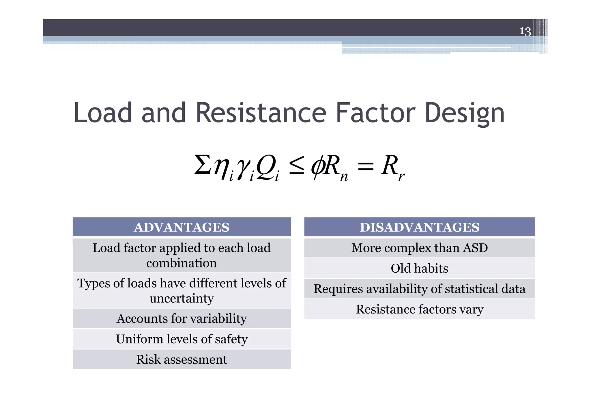
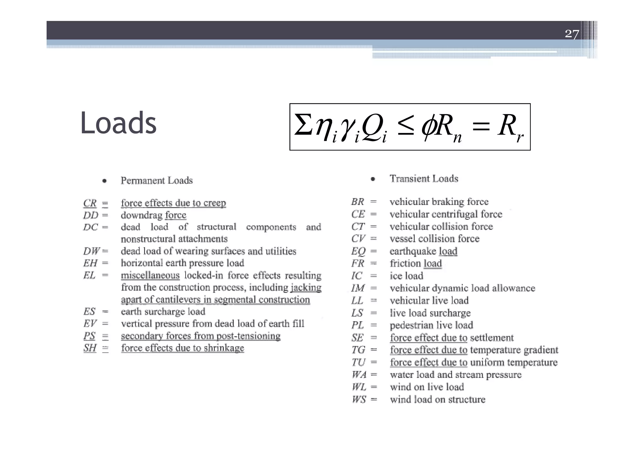
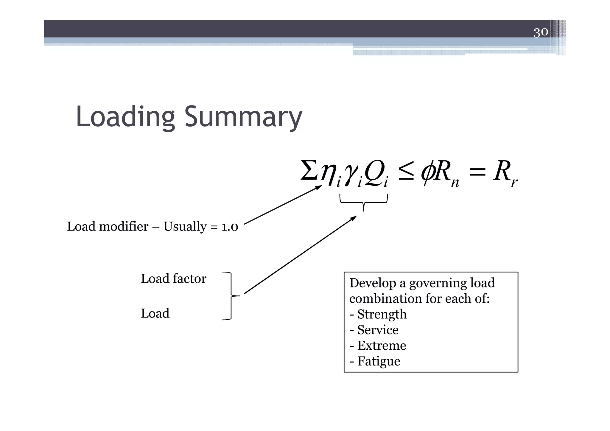
Load and ResistanceFactor Design
Σηiγ i Qi ≤ φRn = Rr
ADVANTAGES DISADVANTAGES
Load factor applied to each load More complex than ASD
combination Old habits
Types of loads have different levels of Requires availability of statistical data
uncertainty
Resistance factors vary
Accounts for variability
Uniform levels of safety
Risk assessment
14.
14
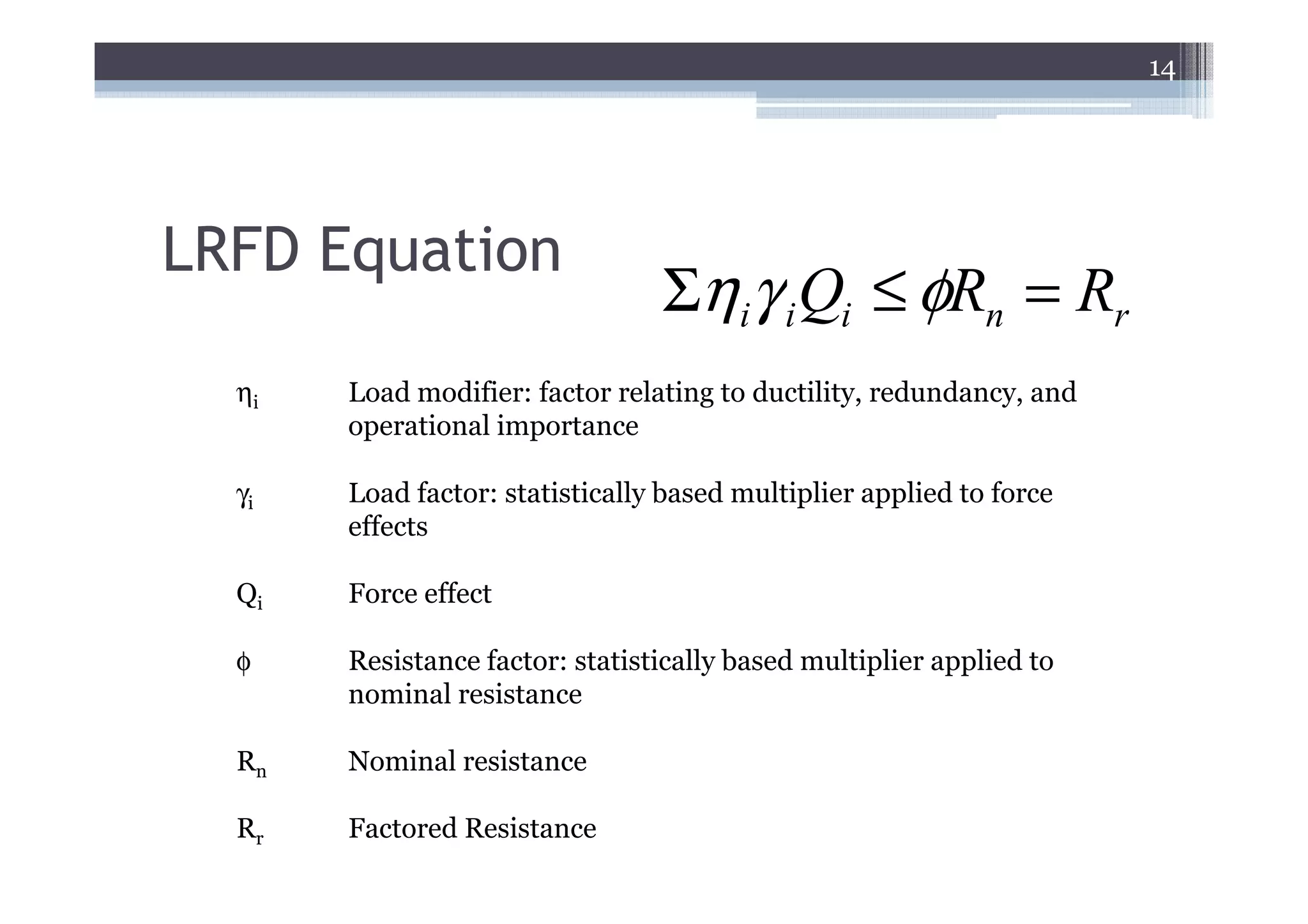
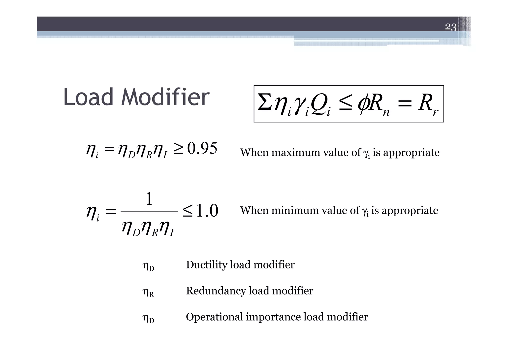
LRFD Equation
Σηiγ i Qi ≤ φRn = Rr
ηi Load modifier: factor relating to ductility, redundancy, and
operational importance
γi Load factor: statistically based multiplier applied to force
effects
Qi Force effect
φ Resistance factor: statistically based multiplier applied to
nominal resistance
Rn Nominal resistance
Rr Factored Resistance
15.
15
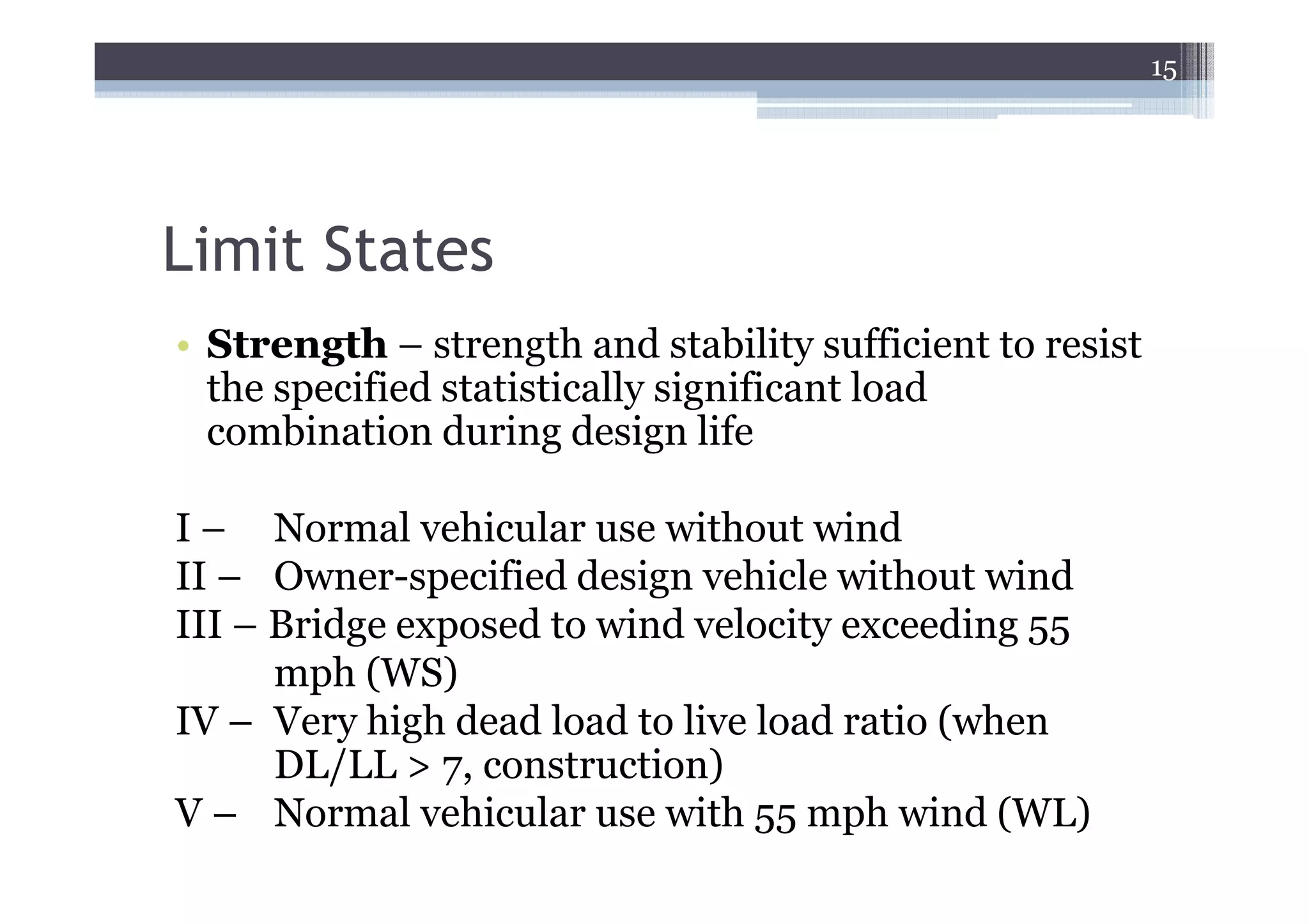
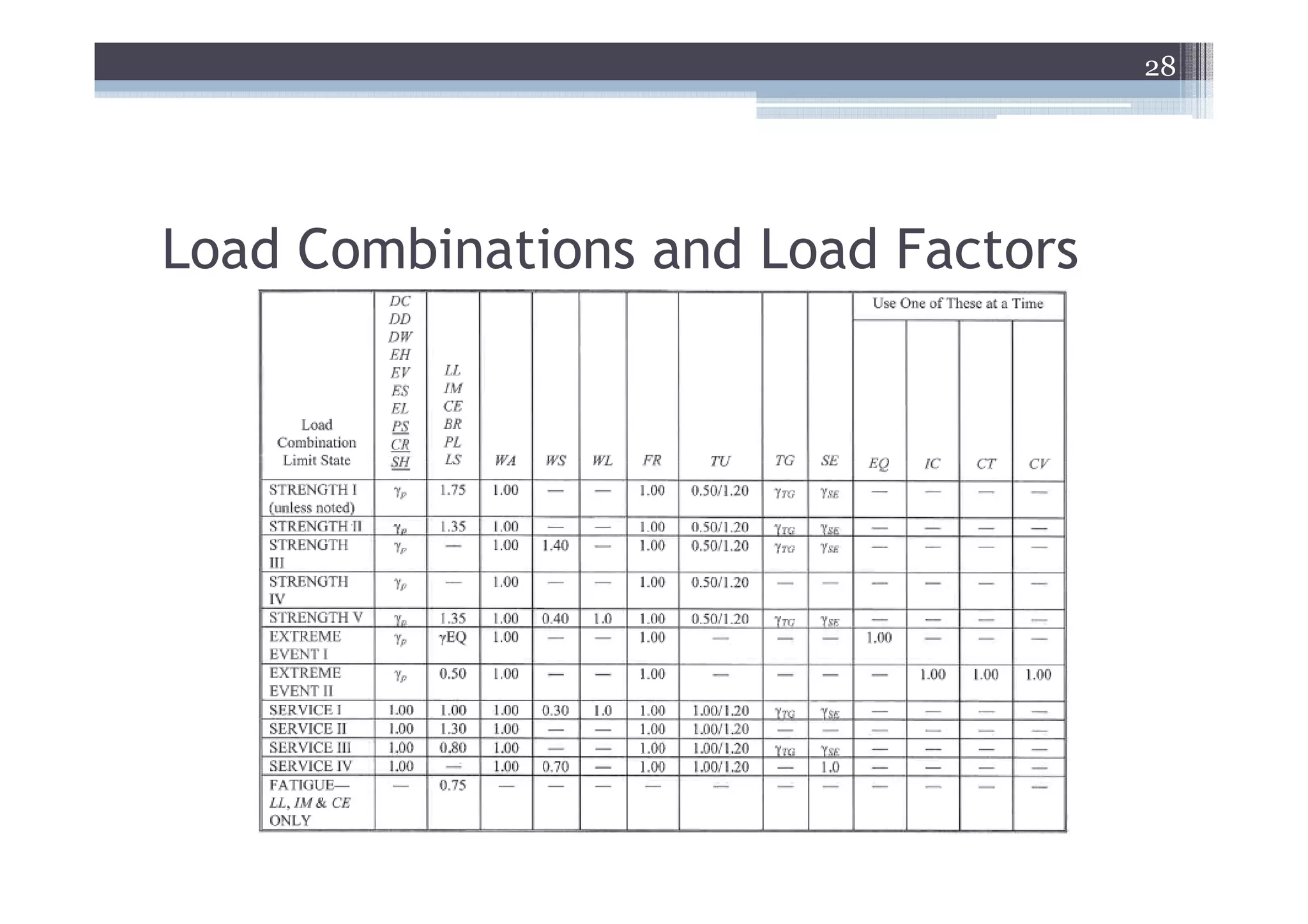
Limit States
• Strength– strength and stability sufficient to resist
the specified statistically significant load
combination during design life
I – Normal vehicular use without wind
II – Owner-specified design vehicle without wind
III – Bridge exposed to wind velocity exceeding 55
mph (WS)
IV – Very high dead load to live load ratio (when
DL/LL > 7, construction)
V – Normal vehicular use with 55 mph wind (WL)
17
Limit States
• Service– Restrictions on stress, deformation, and
crack width under regular service conditions
I– Normal operational use with 55 mph wind.
Also related to deflection control in tunnels,
slopes, etc.
II – Yielding of steel structures and slip of slip-
critical connections due to vehicular live load
III – Longitudinal analysis relating to tension in
prestressed concrete
IV – Relating to crack control from tension in
concrete columns
23
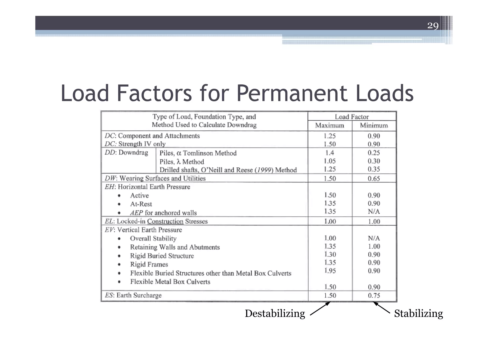
Load Modifier Σηiγ i Qi ≤ φRn = Rr
ηi = η Dη Rη I ≥ 0.95 When maximum value of γi is appropriate
1
ηi = ≤ 1.0 When minimum value of γi is appropriate
η Dη Rη I
ηD Ductility load modifier
ηR Redundancy load modifier
ηD Operational importance load modifier
24.
24
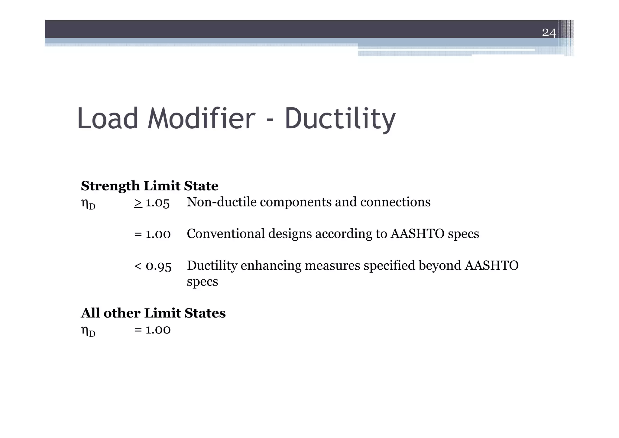
Load Modifier -Ductility
Strength Limit State
ηD > 1.05 Non-ductile components and connections
= 1.00 Conventional designs according to AASHTO specs
< 0.95 Ductility enhancing measures specified beyond AASHTO
specs
All other Limit States
ηD = 1.00
25.
25
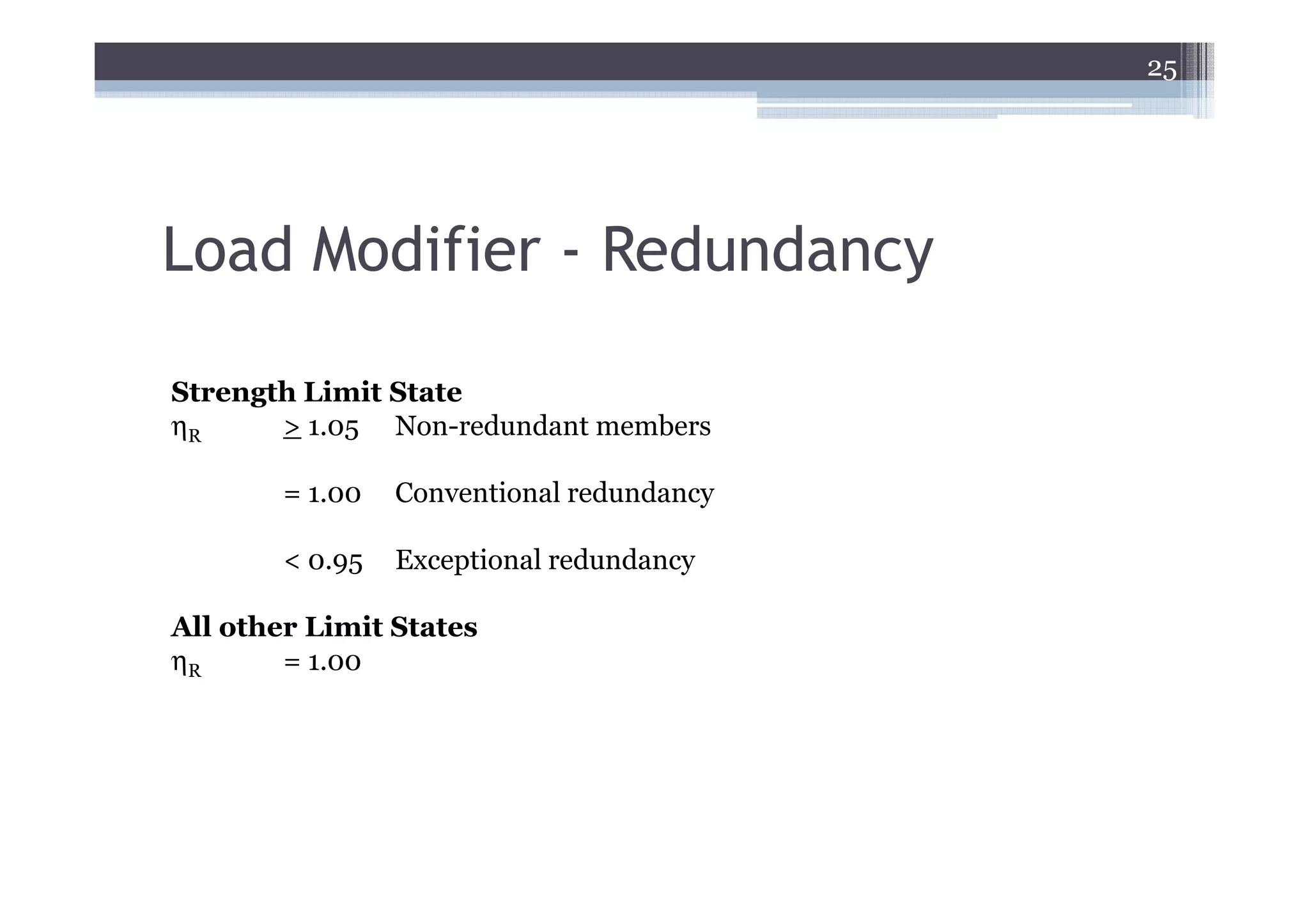
Load Modifier -Redundancy
Strength Limit State
ηR > 1.05 Non-redundant members
= 1.00 Conventional redundancy
< 0.95 Exceptional redundancy
All other Limit States
ηR = 1.00
26.
26
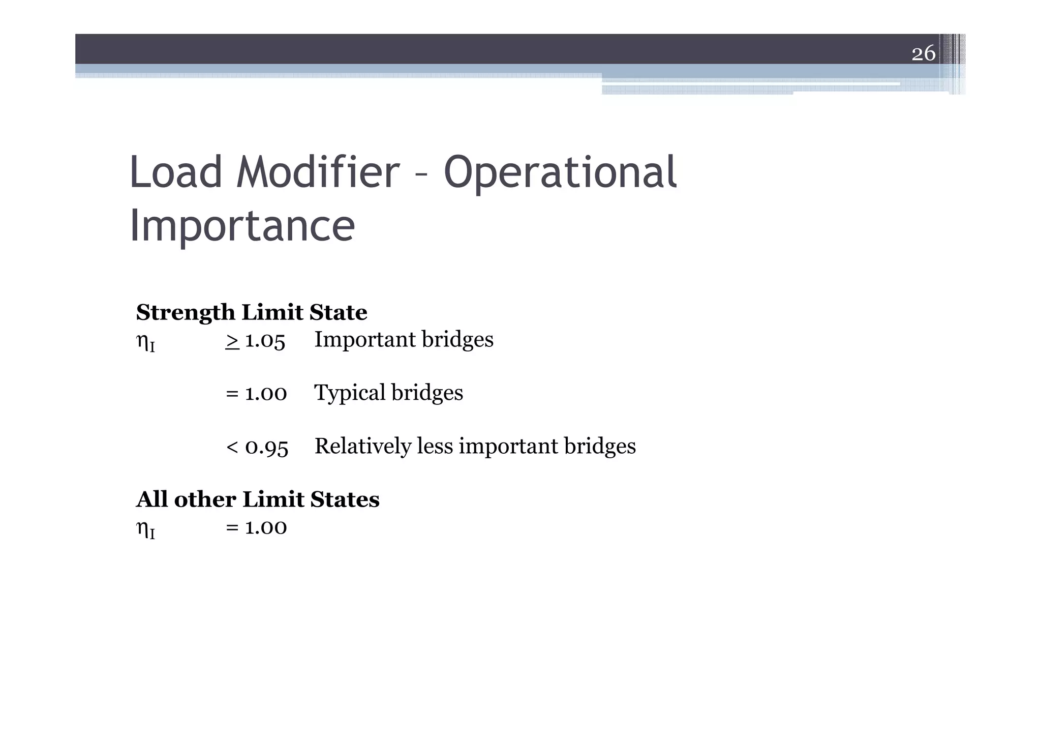
Load Modifier –Operational
Importance
Strength Limit State
ηI > 1.05 Important bridges
= 1.00 Typical bridges
< 0.95 Relatively less important bridges
All other Limit States
ηI = 1.00
39
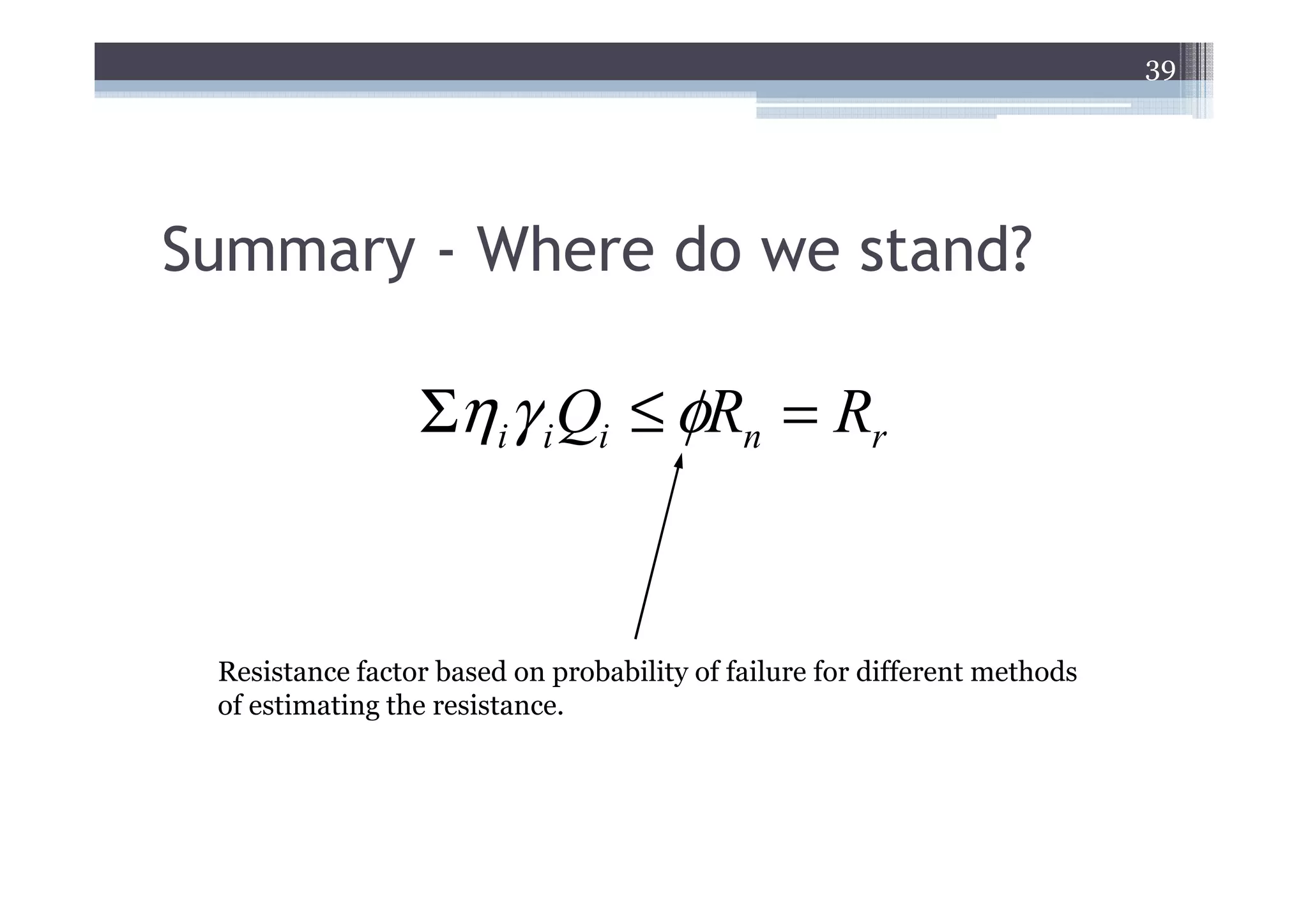
Summary - Wheredo we stand?
Σηiγ i Qi ≤ φRn = Rr
Resistance factor based on probability of failure for different methods
of estimating the resistance.
40.
40
Limit States asApplied to Deep
Foundations
• AASHTO, Section 10.5
• Service Limits
• Strength Limits
• Extreme Limits
41.
41
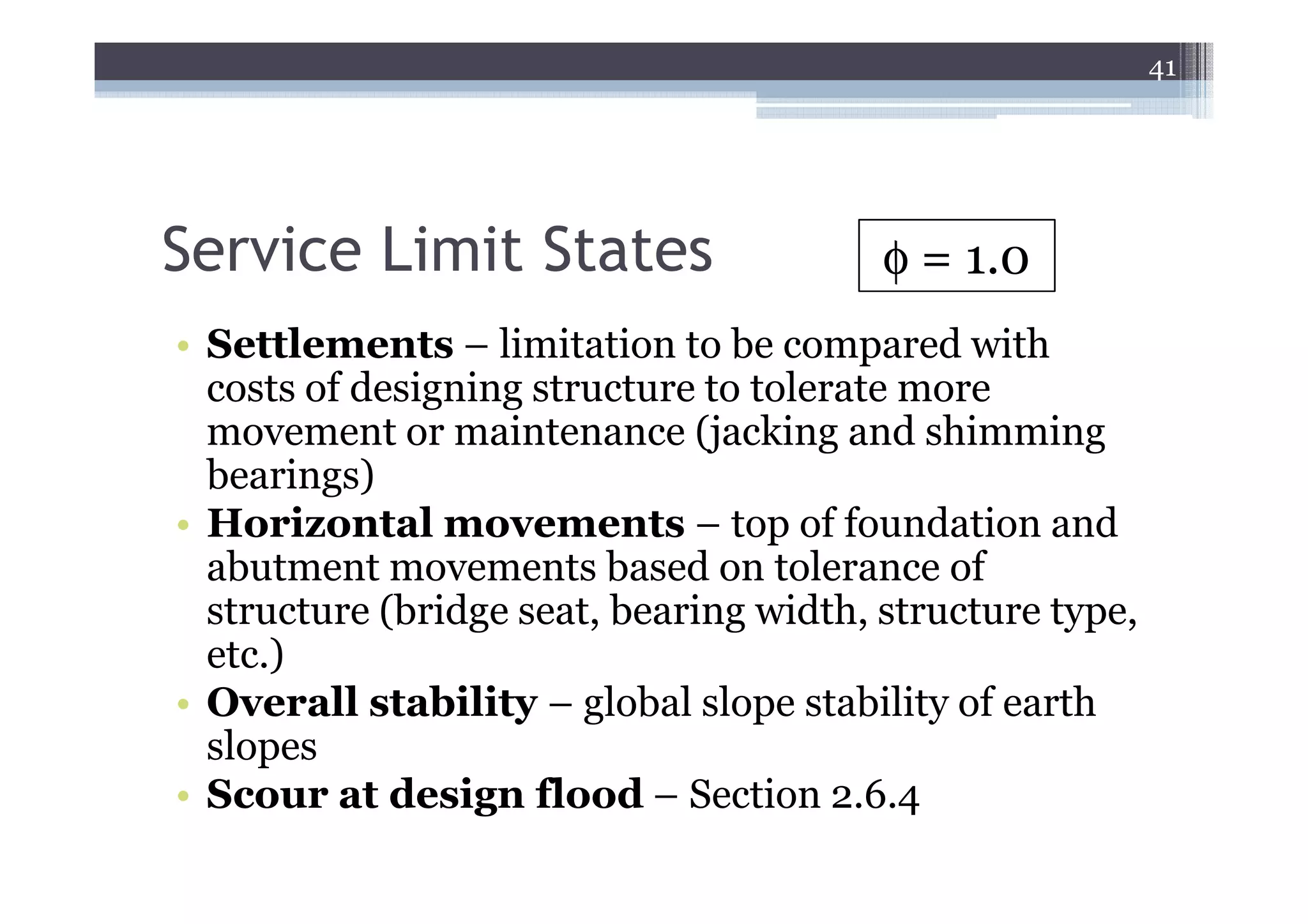
Service Limit States φ = 1.0
• Settlements – limitation to be compared with
costs of designing structure to tolerate more
movement or maintenance (jacking and shimming
bearings)
• Horizontal movements – top of foundation and
abutment movements based on tolerance of
structure (bridge seat, bearing width, structure type,
etc.)
• Overall stability – global slope stability of earth
slopes
• Scour at design flood – Section 2.6.4
42.
42
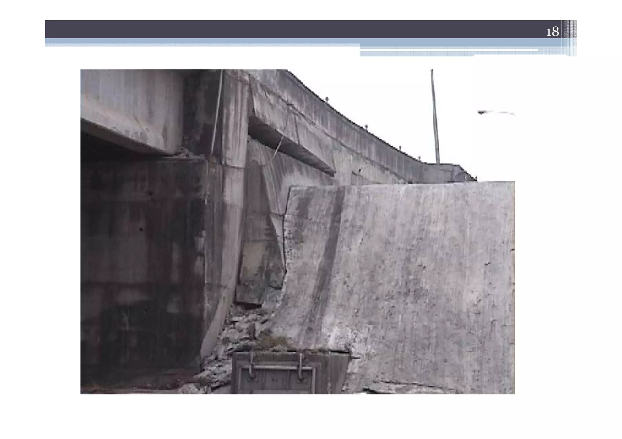
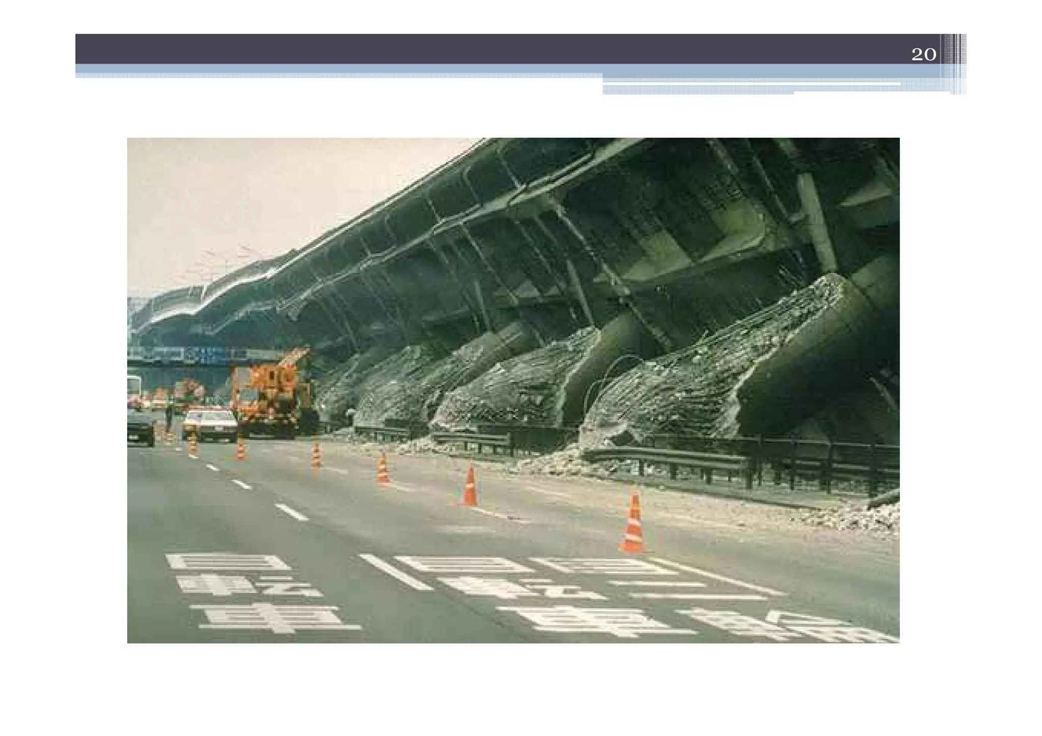
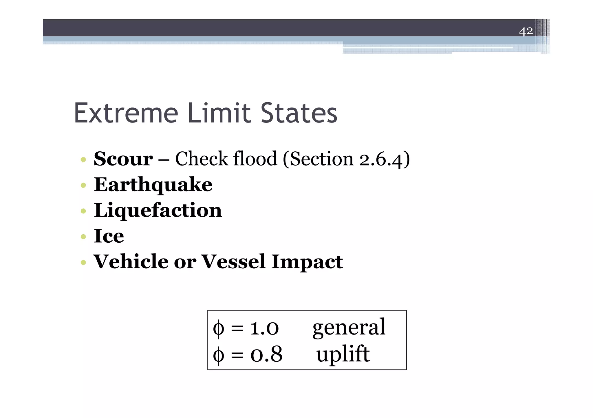
Extreme Limit States
• Scour – Check flood (Section 2.6.4)
• Earthquake
• Liquefaction
• Ice
• Vehicle or Vessel Impact
φ = 1.0 general
φ = 0.8 uplift
43.
43
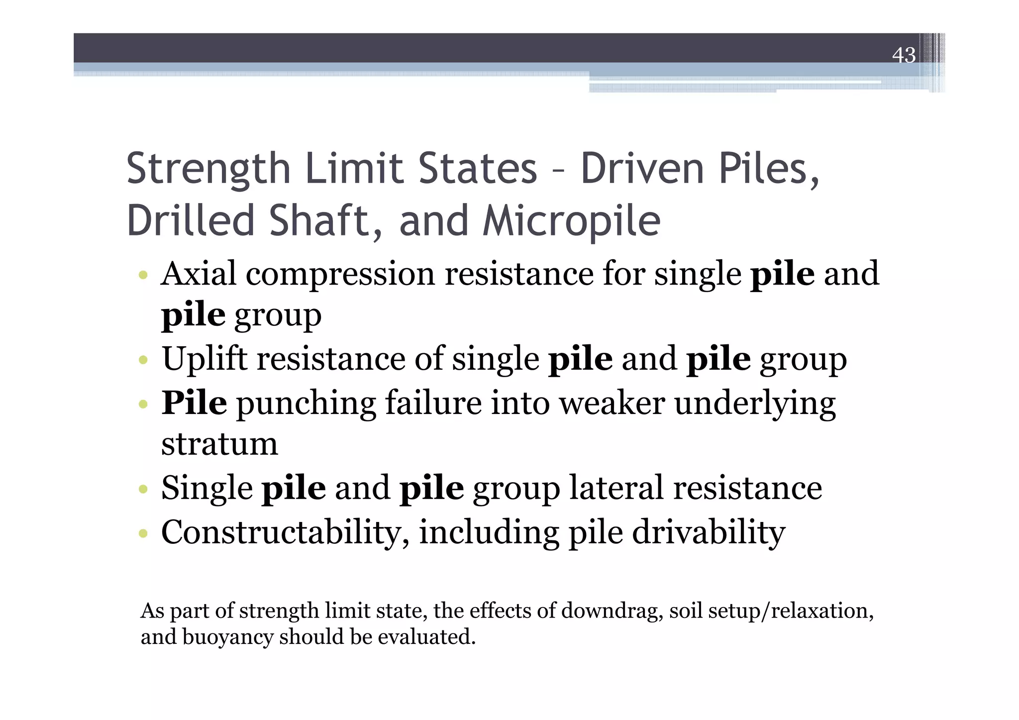
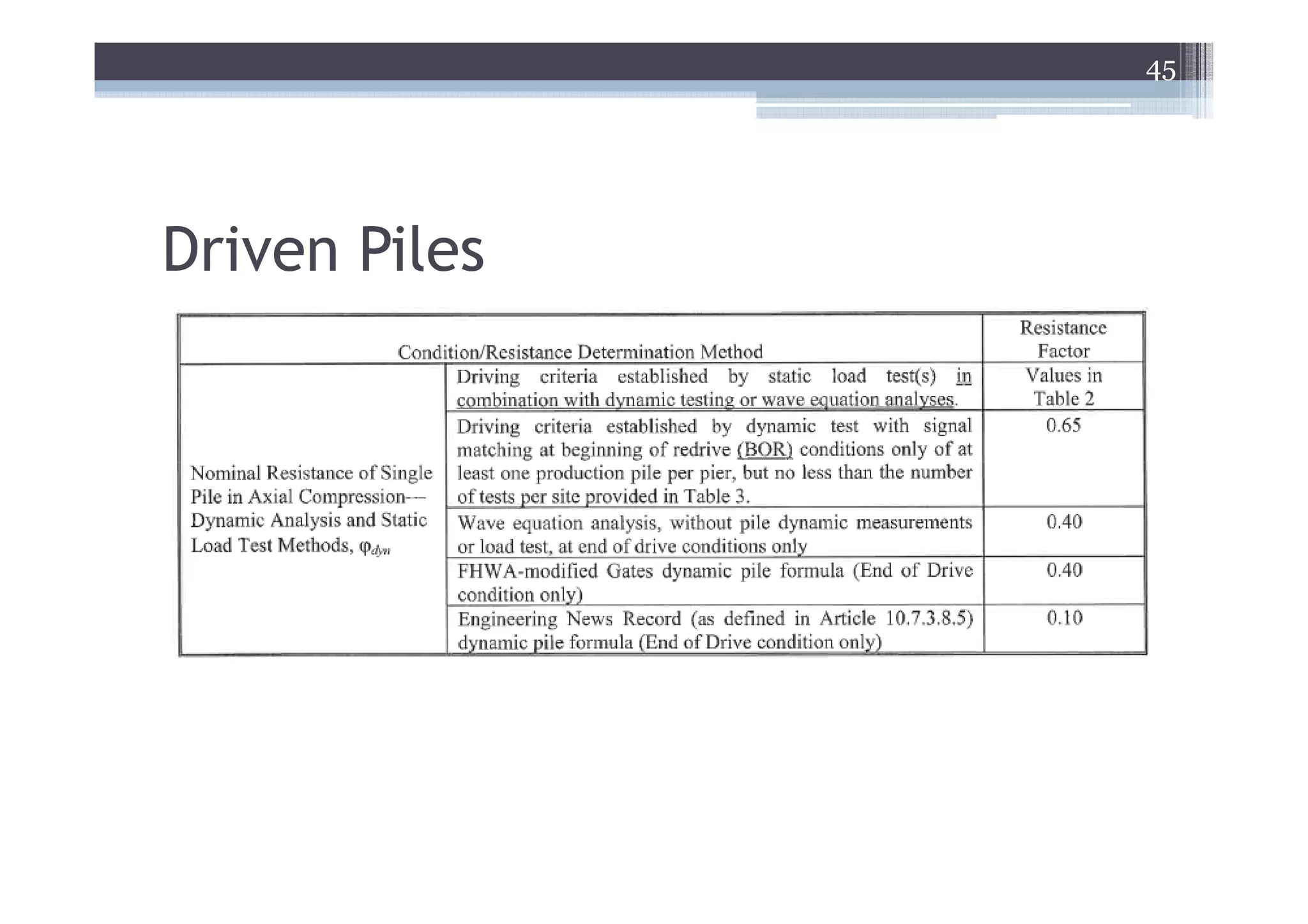
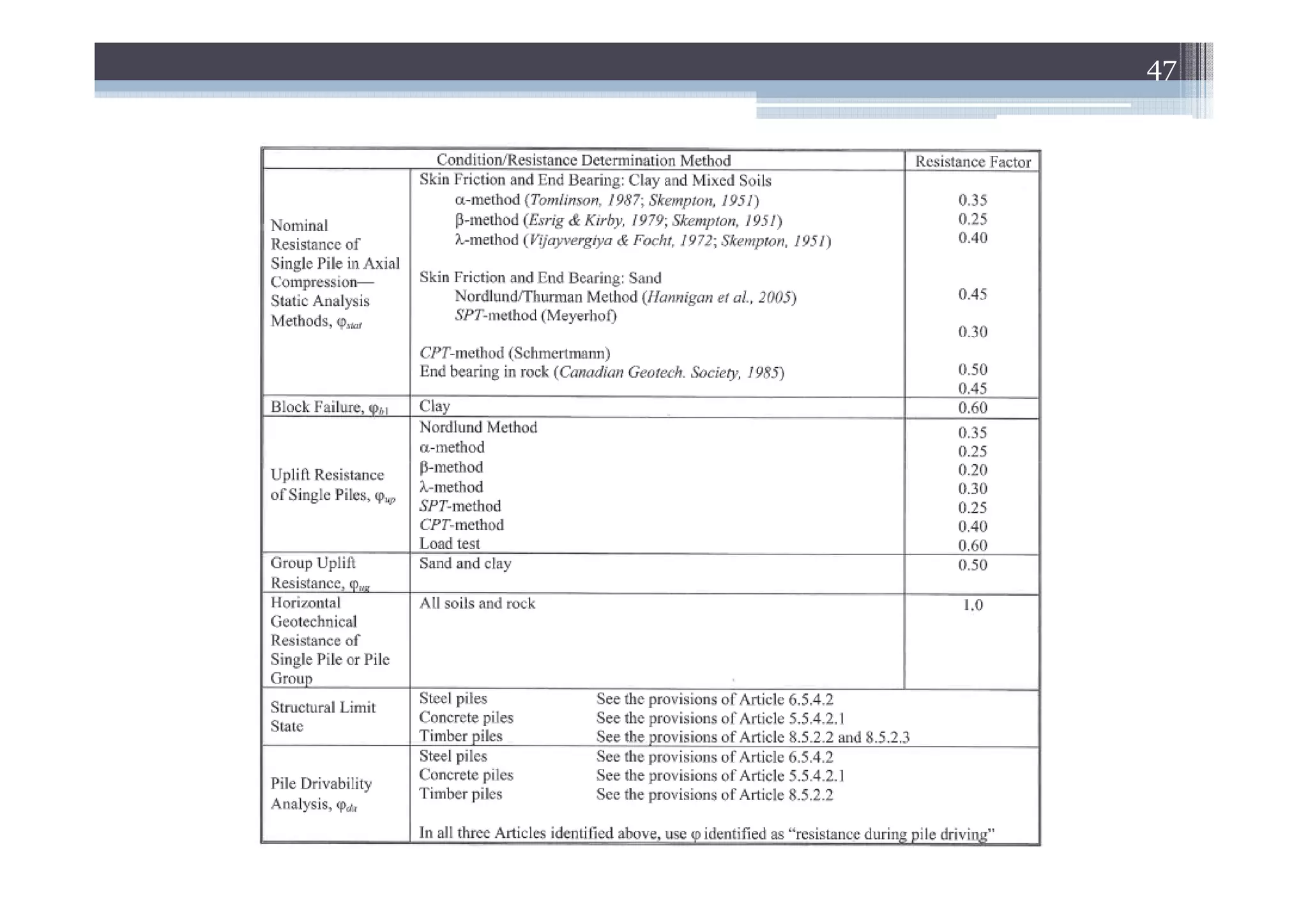
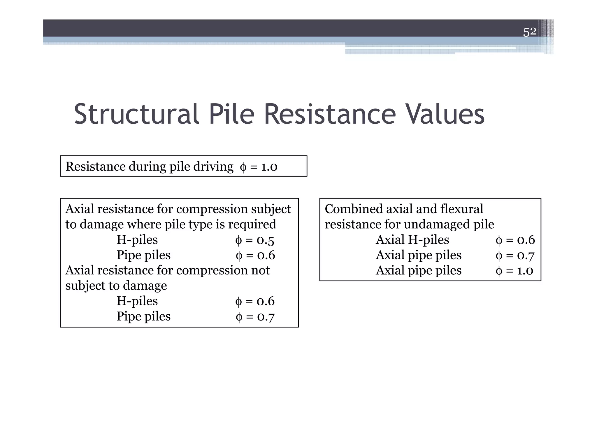
Strength Limit States– Driven Piles,
Drilled Shaft, and Micropile
• Axial compression resistance for single pile and
pile group
• Uplift resistance of single pile and pile group
• Pile punching failure into weaker underlying
stratum
• Single pile and pile group lateral resistance
• Constructability, including pile drivability
As part of strength limit state, the effects of downdrag, soil setup/relaxation,
and buoyancy should be evaluated.
44.
44
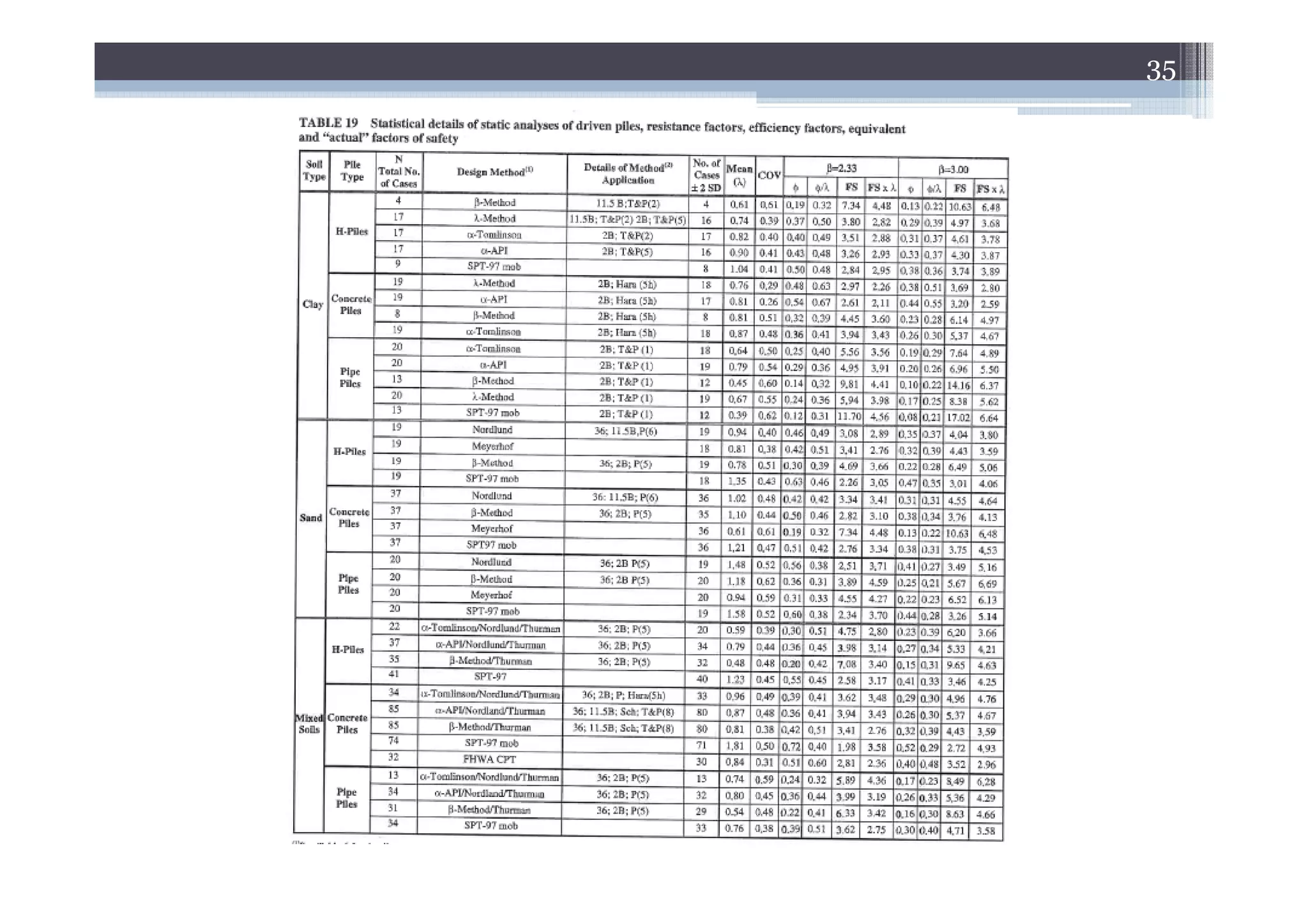
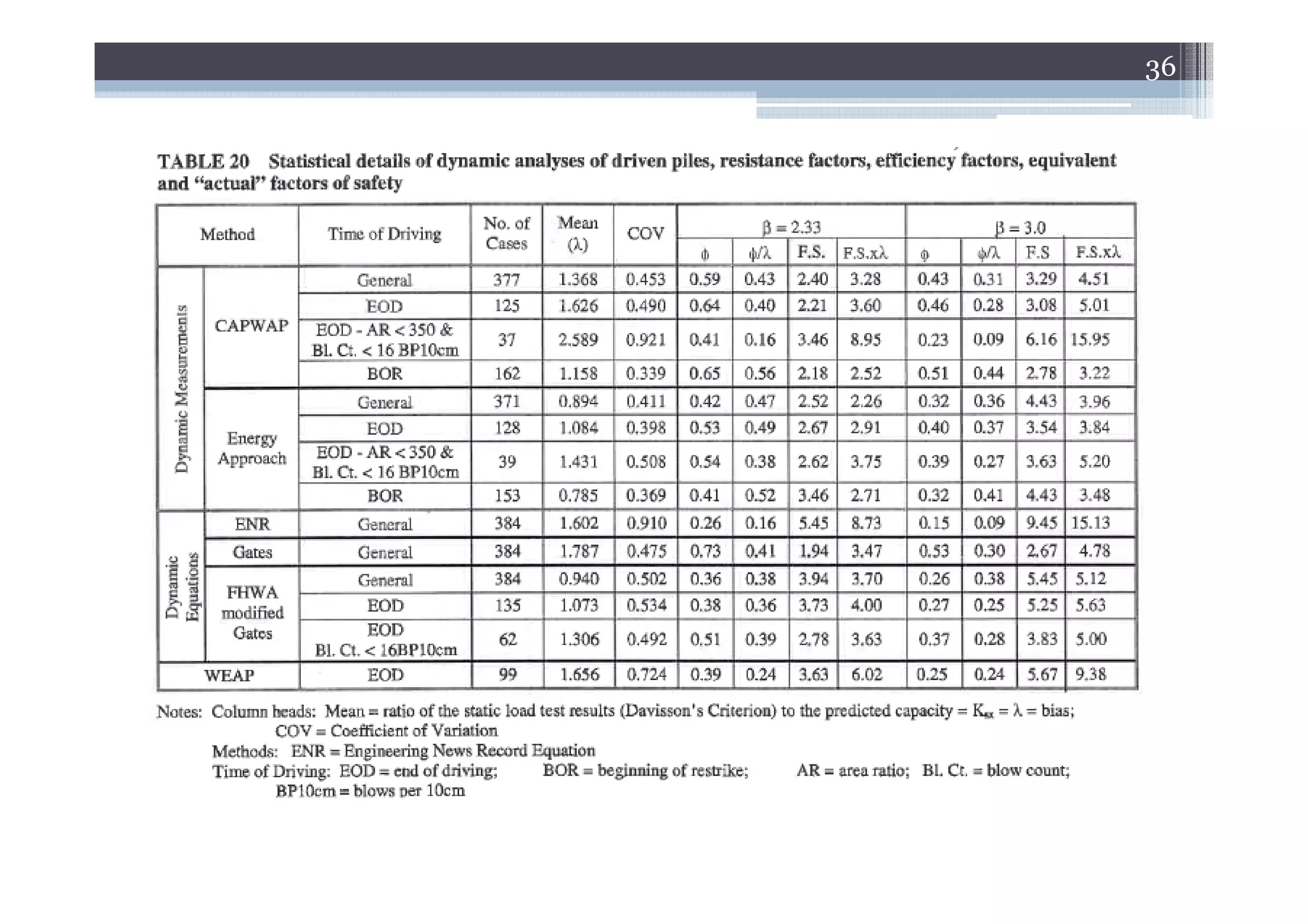
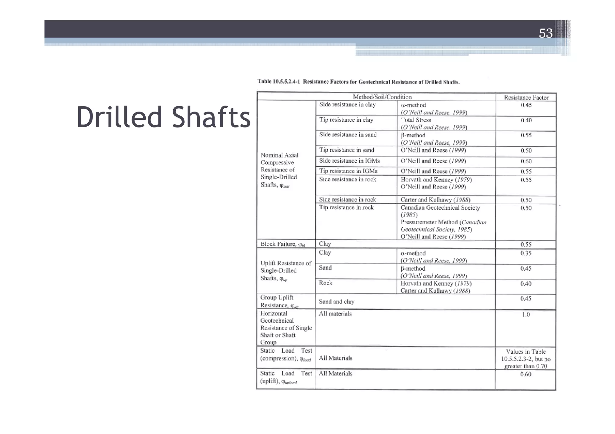
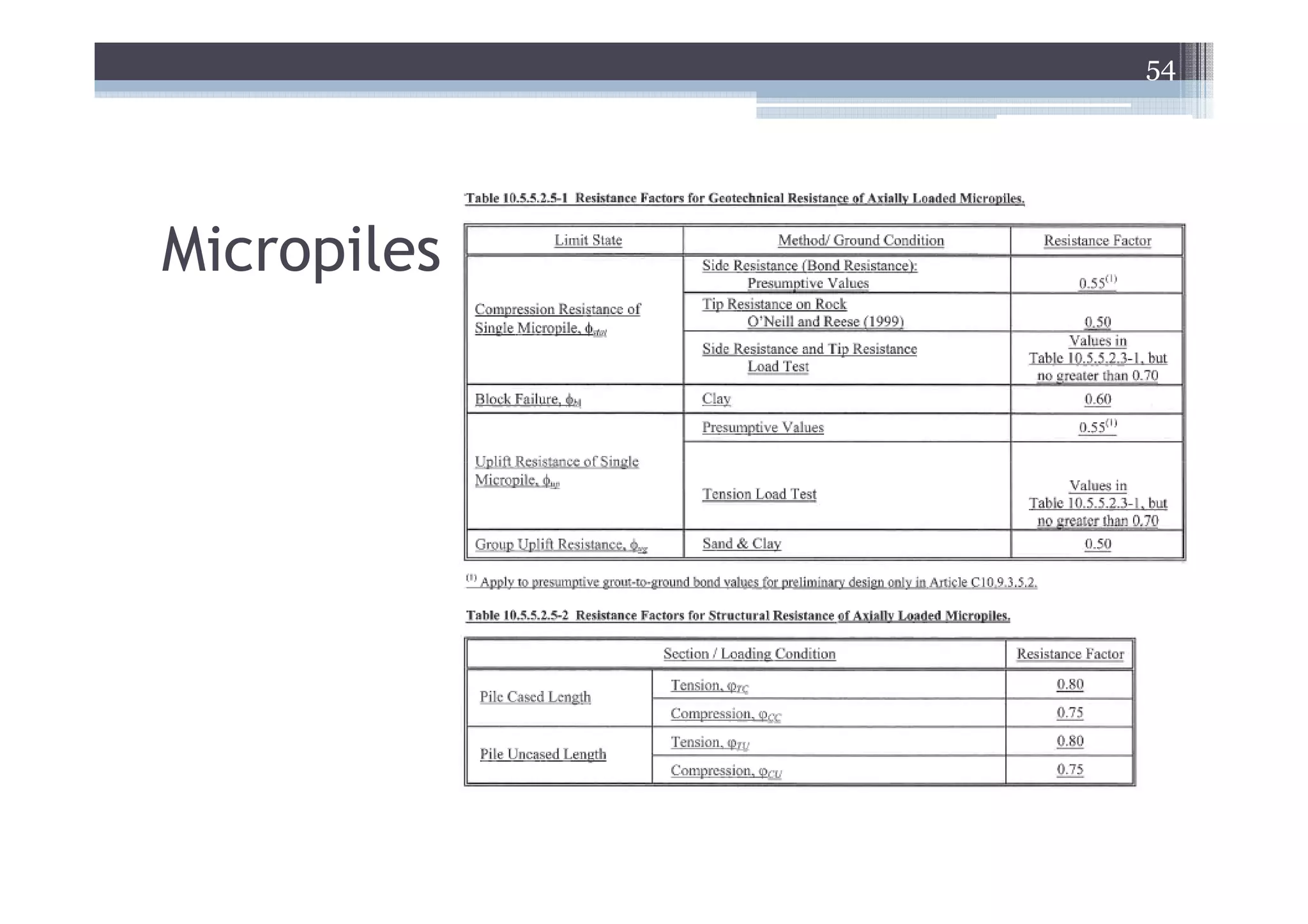
Strength Limit ResistanceFactors
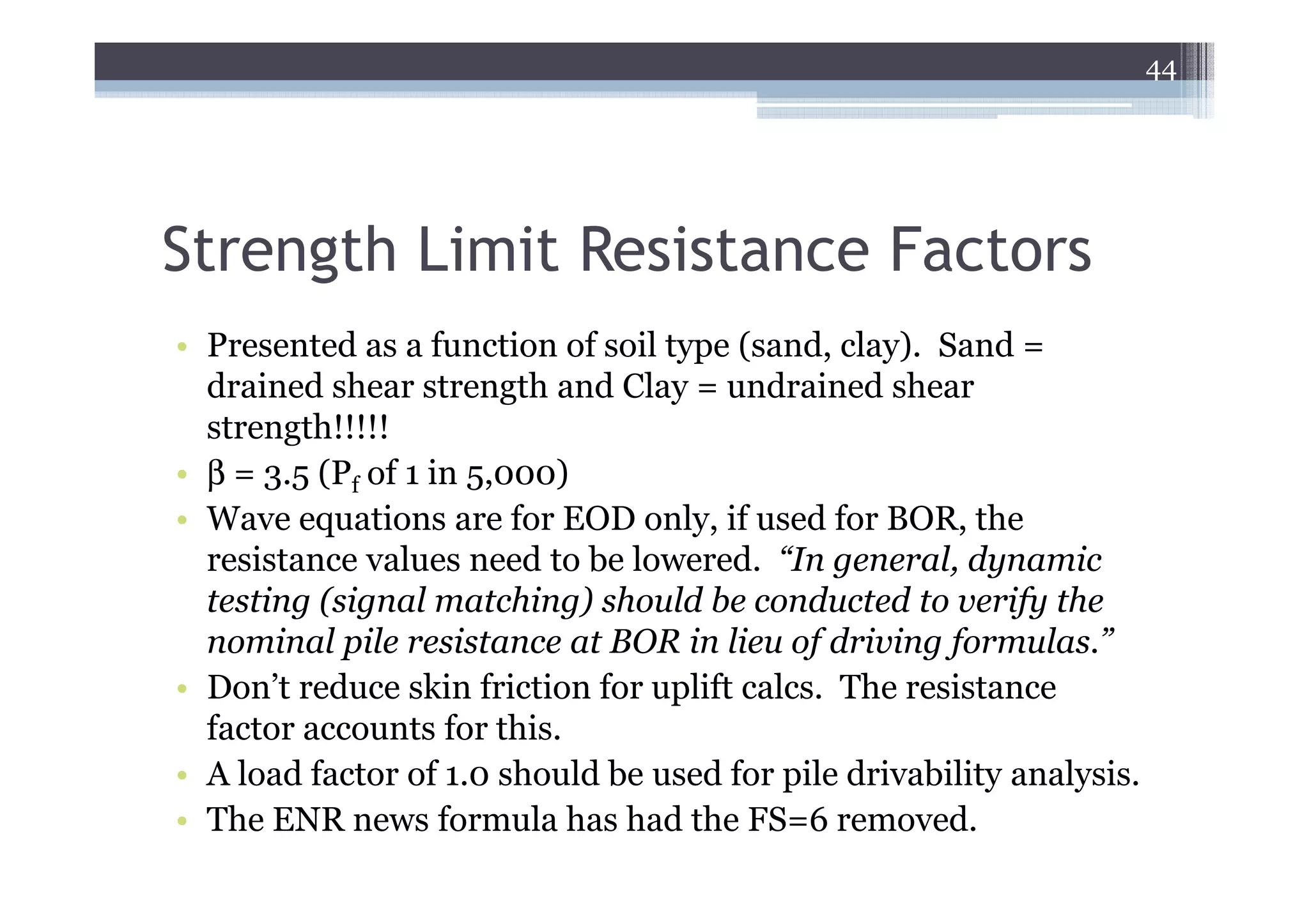
• Presented as a function of soil type (sand, clay). Sand =
drained shear strength and Clay = undrained shear
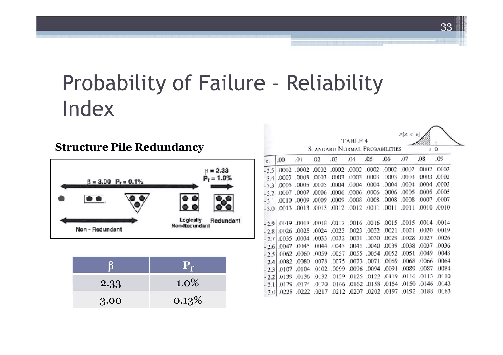
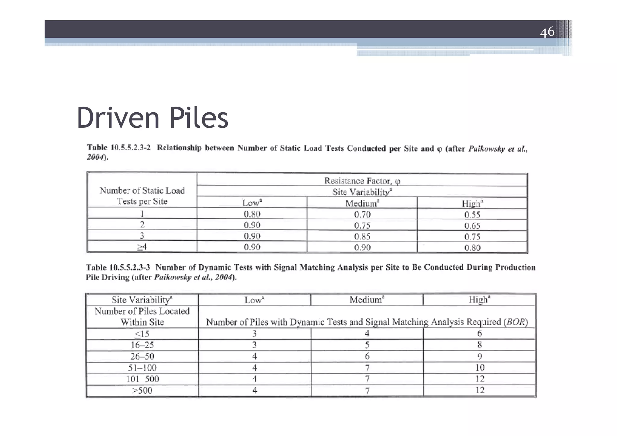
strength!!!!!
• β = 3.5 (Pf of 1 in 5,000)
• Wave equations are for EOD only, if used for BOR, the
resistance values need to be lowered. “In general, dynamic
testing (signal matching) should be conducted to verify the
nominal pile resistance at BOR in lieu of driving formulas.”
• Don’t reduce skin friction for uplift calcs. The resistance
factor accounts for this.
• A load factor of 1.0 should be used for pile drivability analysis.
• The ENR news formula has had the FS=6 removed.
49
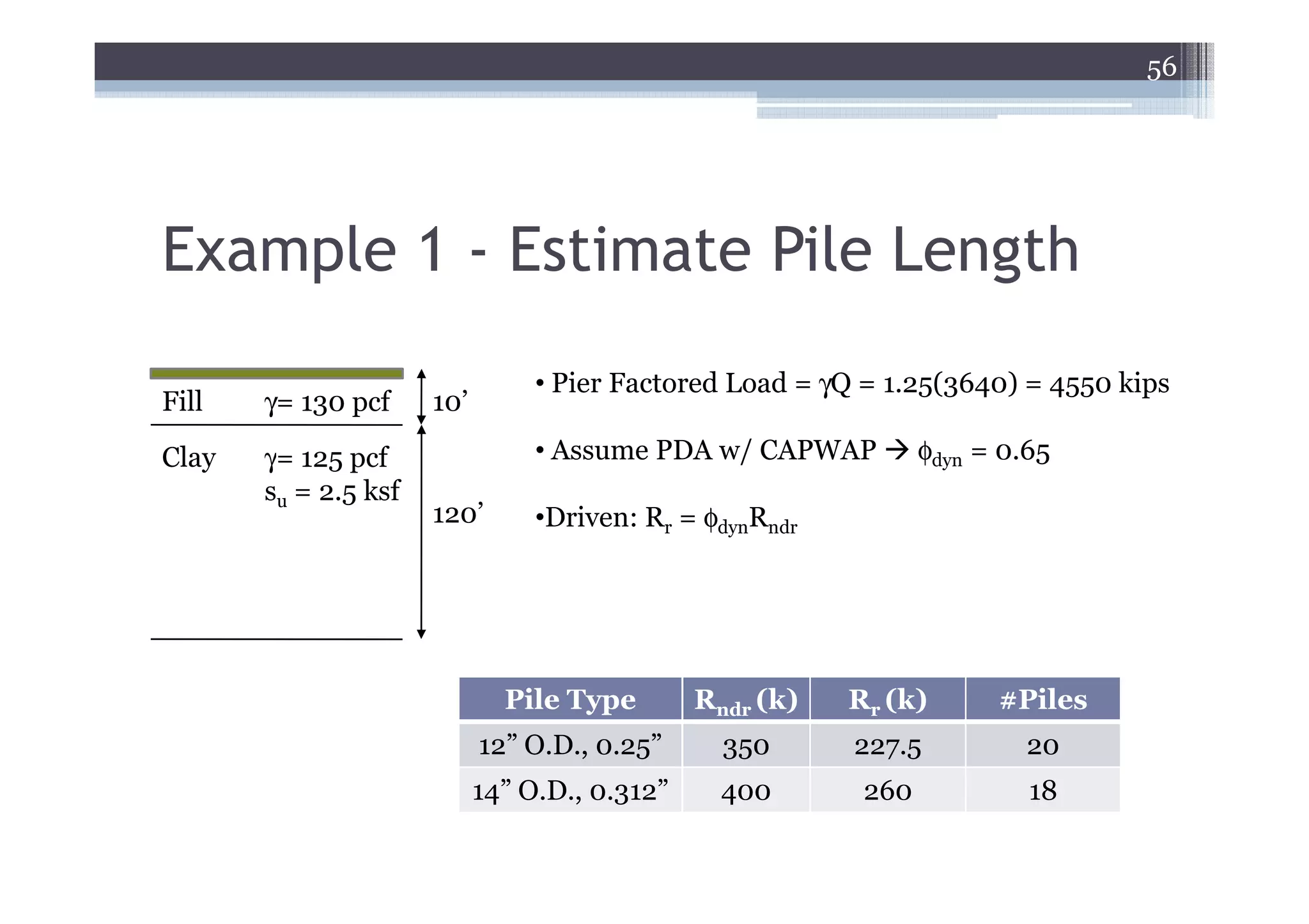
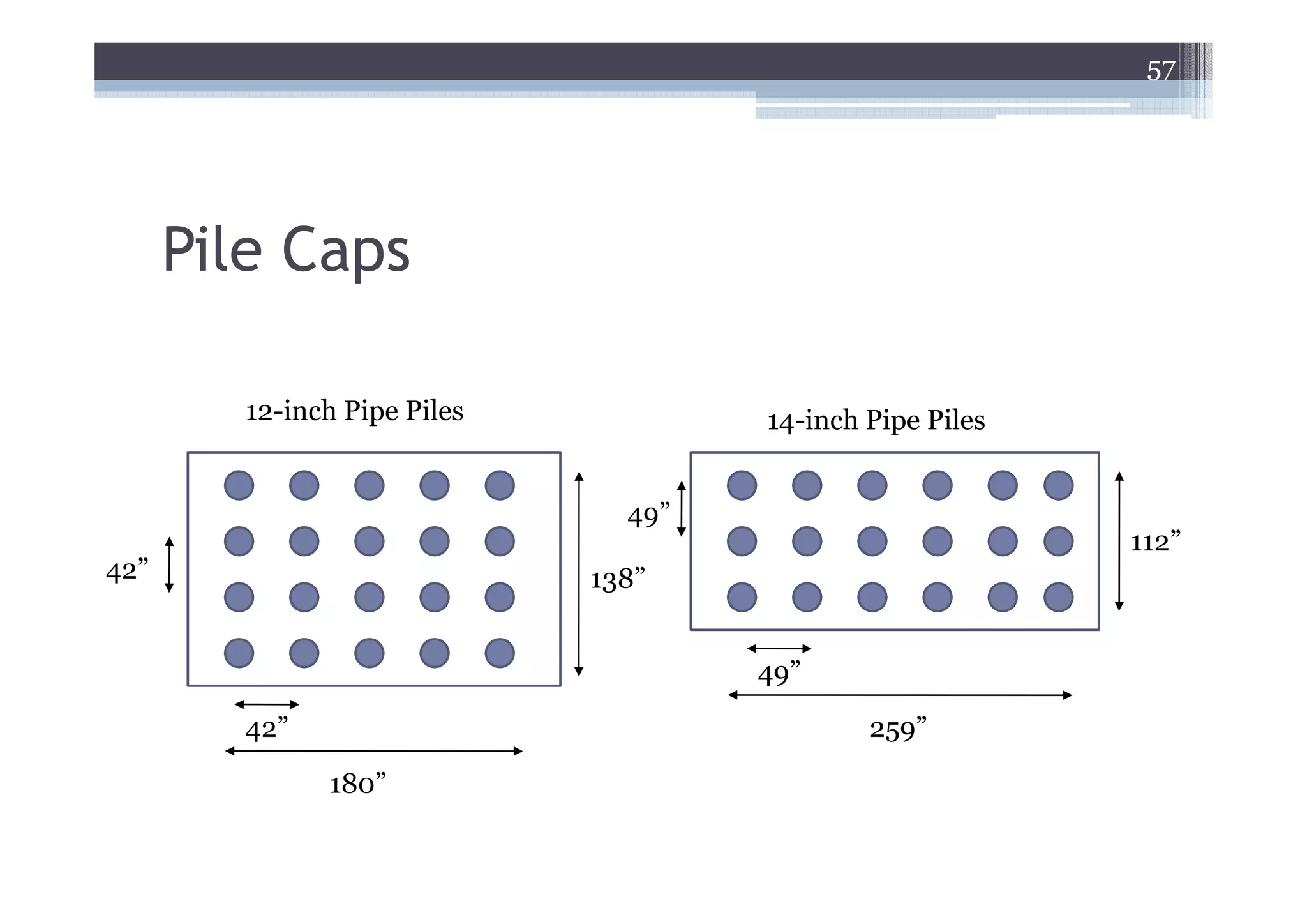
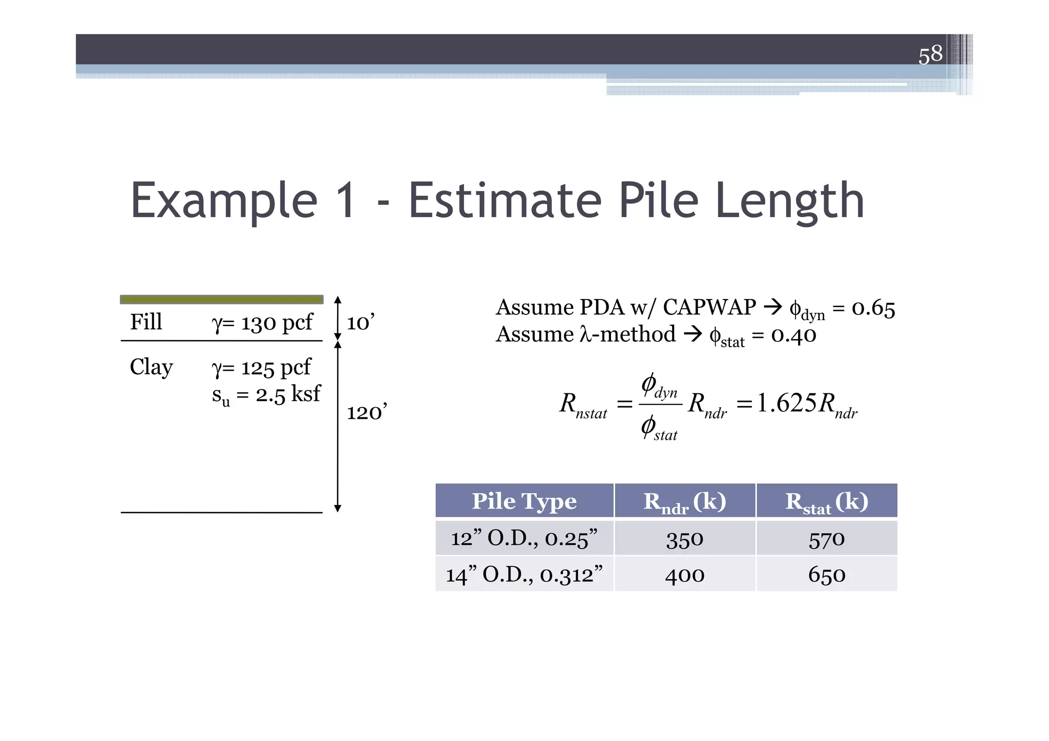
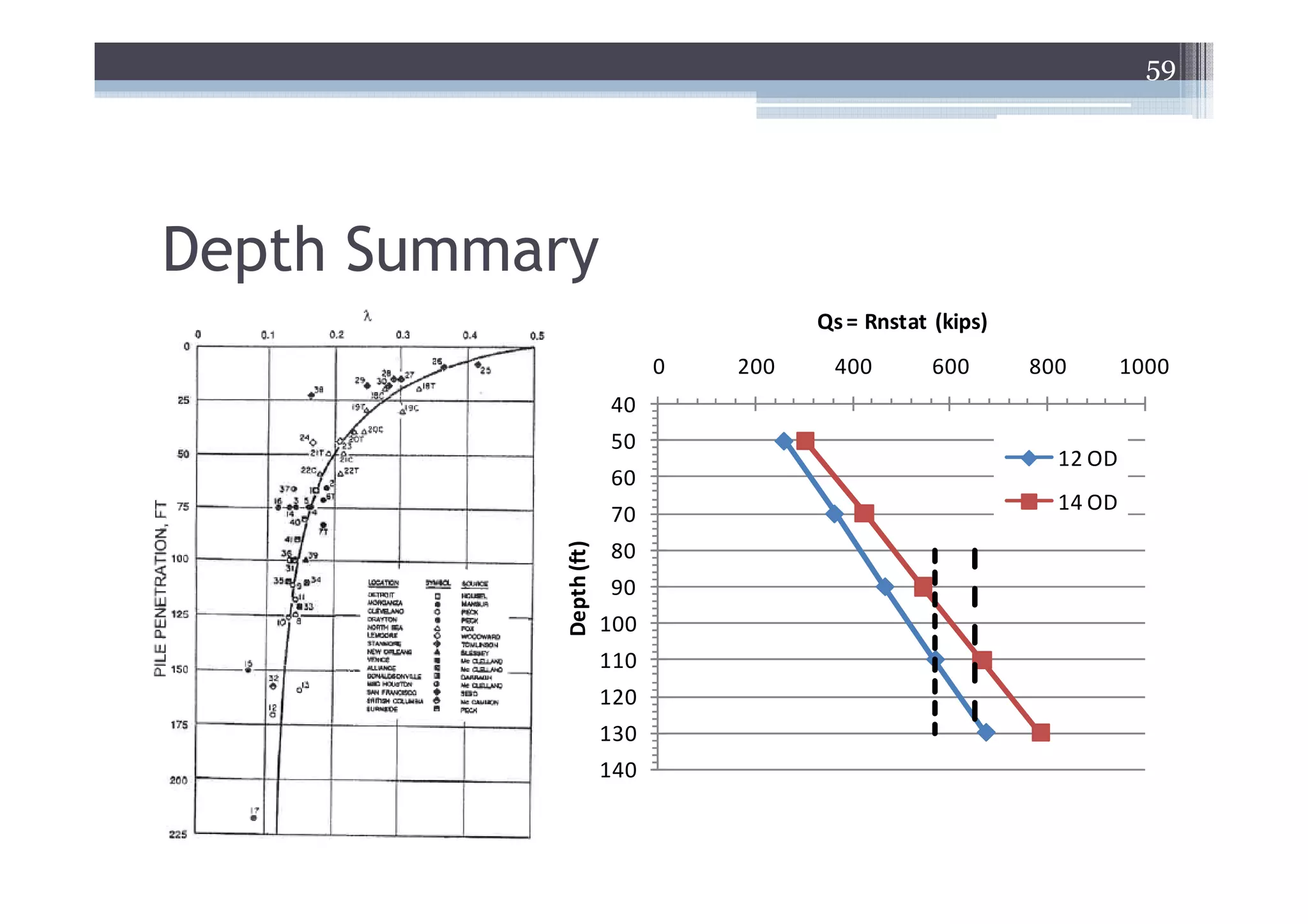
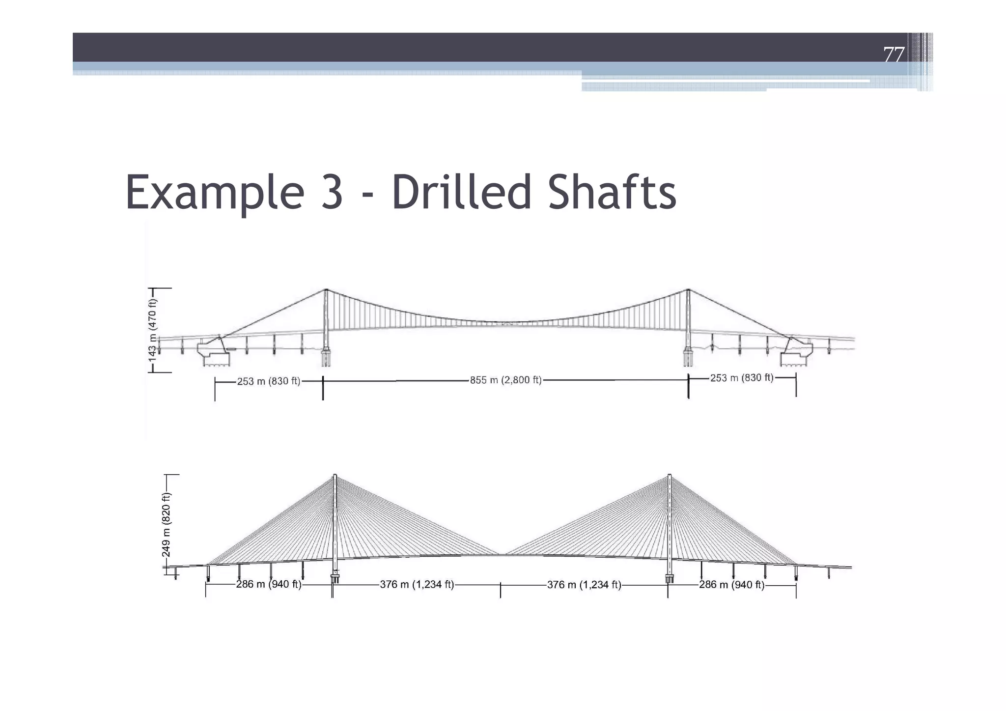
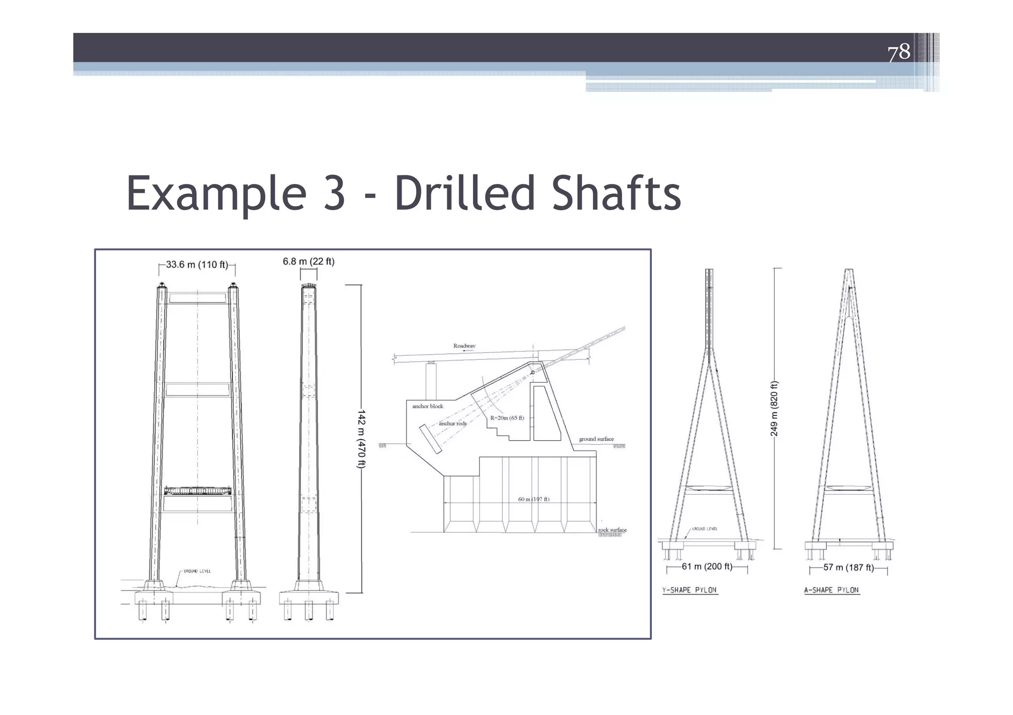
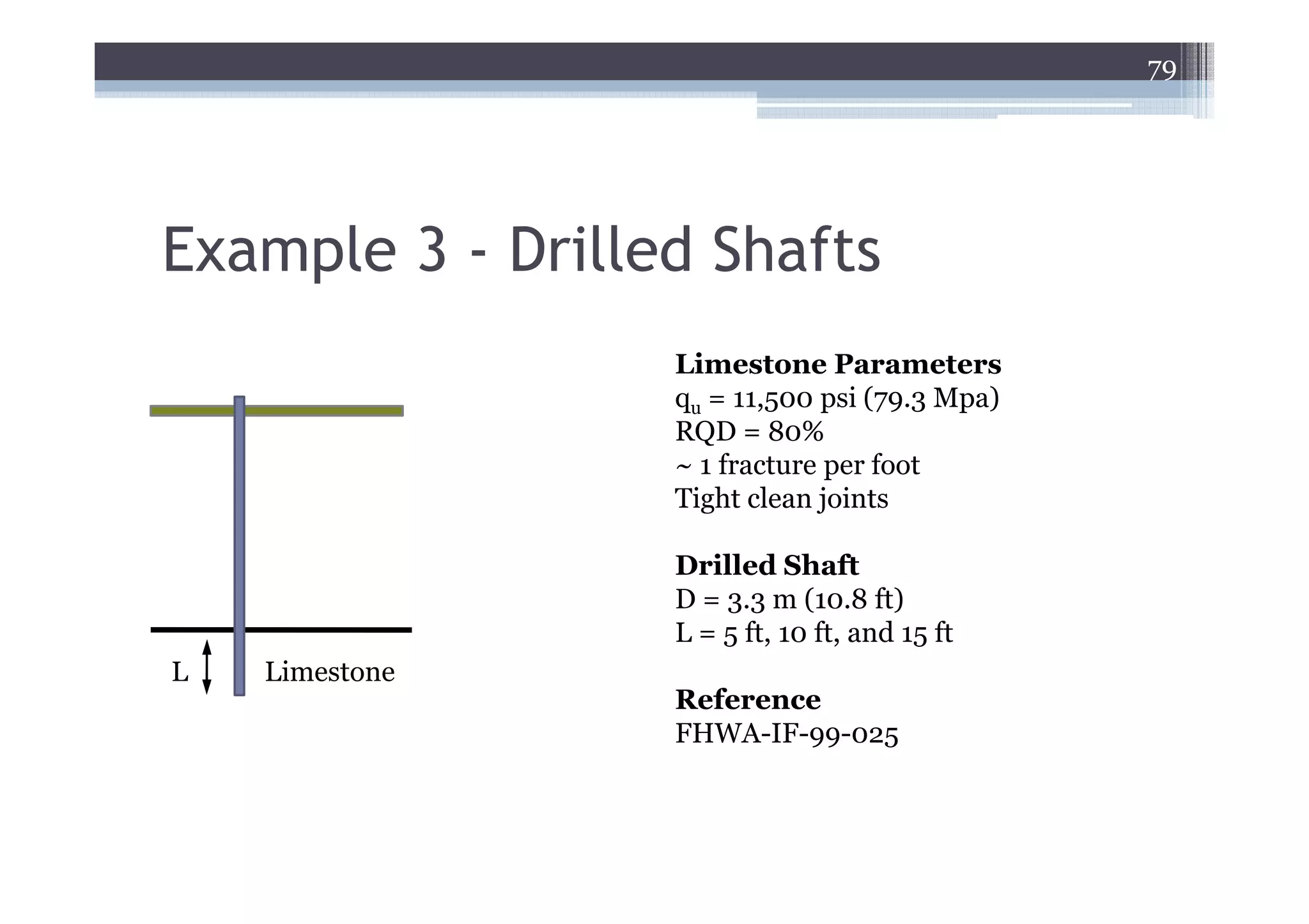
Pile Length Estimatefor Contract
Documents
• Static analysis is only usually used to establish
the pile length estimate for contract documents.
Field testing (e.g., PDA w/ CAPWAP) is used for
driving criteria.
φdyn Rndr = φstat Rnstat
55
Summary
• LRFD –statistically based method to account for
the probability of failure
▫ Compared with ASD
▫ Limit states and resistance
▫ Load factors and combinations
▫ Resistance factors
60
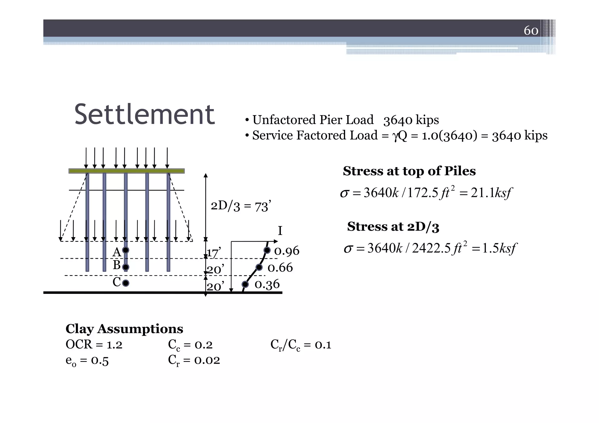
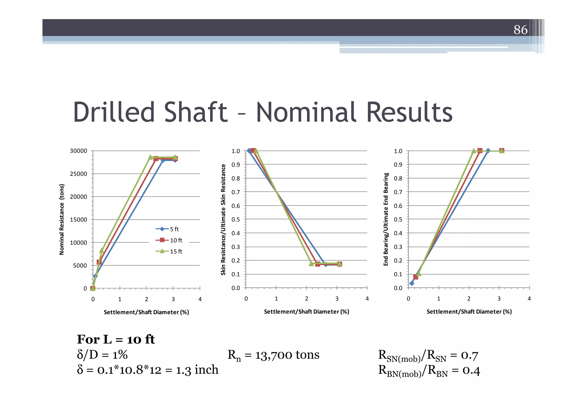
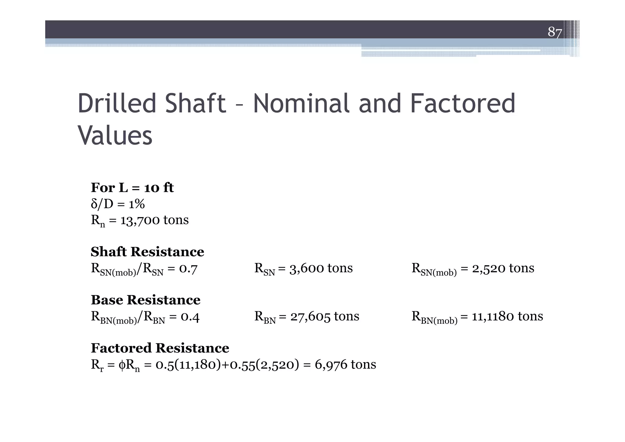
Settlement • Unfactored Pier Load 3640 kips
• Service Factored Load = γQ = 1.0(3640) = 3640 kips
Stress at top of Piles
σ = 3640k / 172.5 ft 2 = 21.1ksf
2D/3 = 73’
I Stress at 2D/3
A 17’ 0.96 σ = 3640k / 2422.5 ft 2 = 1.5ksf
B 20’ 0.66
C 20’ 0.36
Clay Assumptions
OCR = 1.2 Cc = 0.2 Cr/Cc = 0.1
eo = 0.5 Cr = 0.02
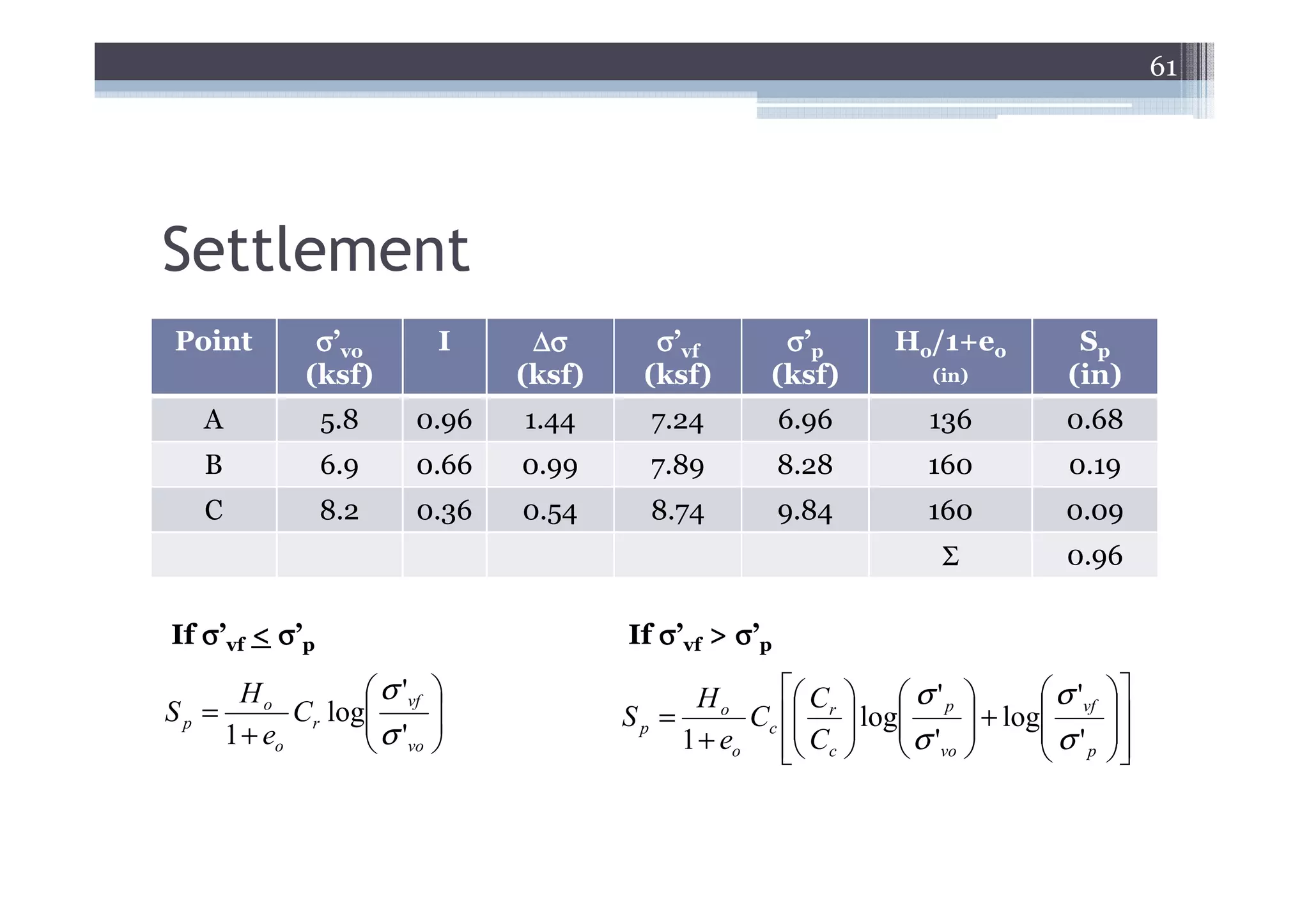
61.
61
Settlement
Point σ’vo I ∆σ σ’vf σ’p Ho/1+eo Sp
(ksf) (ksf) (ksf) (ksf) (in) (in)
A 5.8 0.96 1.44 7.24 6.96 136 0.68
B 6.9 0.66 0.99 7.89 8.28 160 0.19
C 8.2 0.36 0.54 8.74 9.84 160 0.09
Σ 0.96
If σ’vf < σ’p If σ’vf > σ’p
Ho σ 'vf Ho C σ ' p σ 'vf
Sp = Cr log
σ ' Sp =
C σ ' + log σ '
Cc log
r
1 + eo
vo 1 + eo c vo
p
62.
62
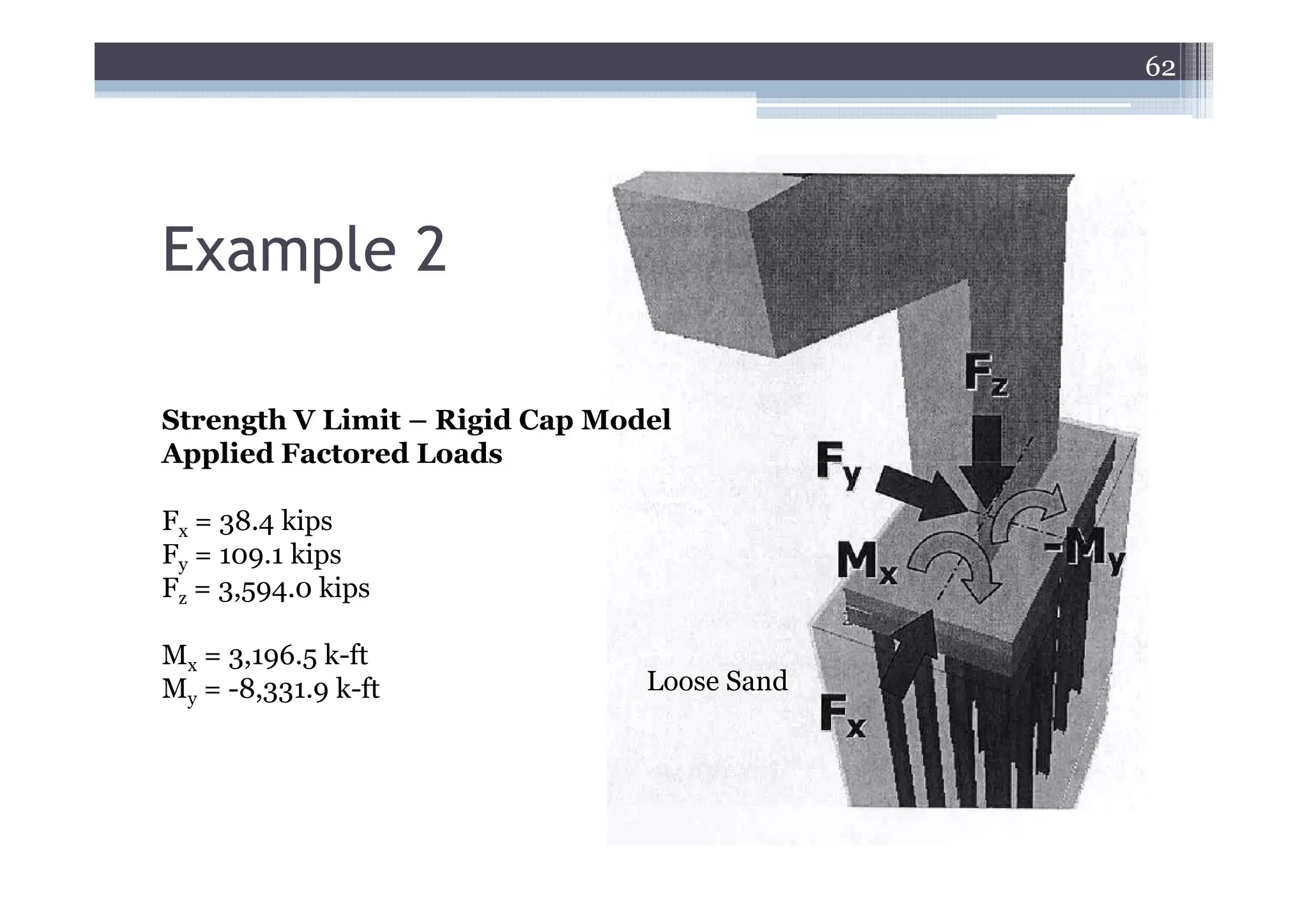
Example 2
Strength VLimit – Rigid Cap Model
Applied Factored Loads
Fx = 38.4 kips
Fy = 109.1 kips
Fz = 3,594.0 kips
Mx = 3,196.5 k-ft
My = -8,331.9 k-ft Loose Sand
63.
63
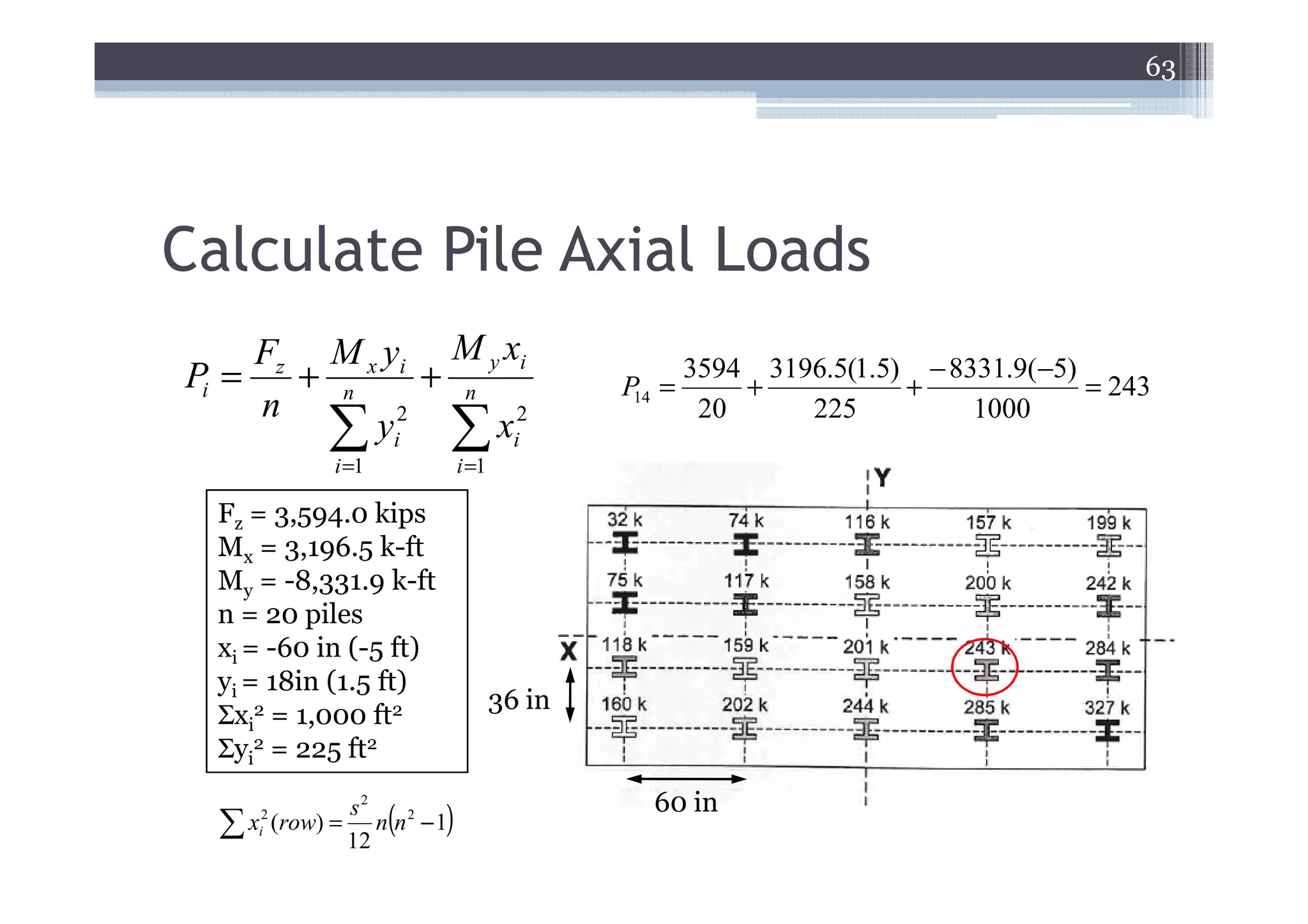
Calculate Pile AxialLoads
Fz M x yi M y xi 3594 3196.5(1.5) − 8331.9(−5)
Pi = + n + n P = + + = 243
n 14
∑ yi2 ∑ xi2
20 225 1000
i =1 i =1
Fz = 3,594.0 kips
Mx = 3,196.5 k-ft
My = -8,331.9 k-ft
n = 20 piles
xi = -60 in (-5 ft)
yi = 18in (1.5 ft)
36 in
Σxi2 = 1,000 ft2
Σyi2 = 225 ft2
60 in
s2
( )
∑ x (row) = 12 n n 2 − 1
2
i
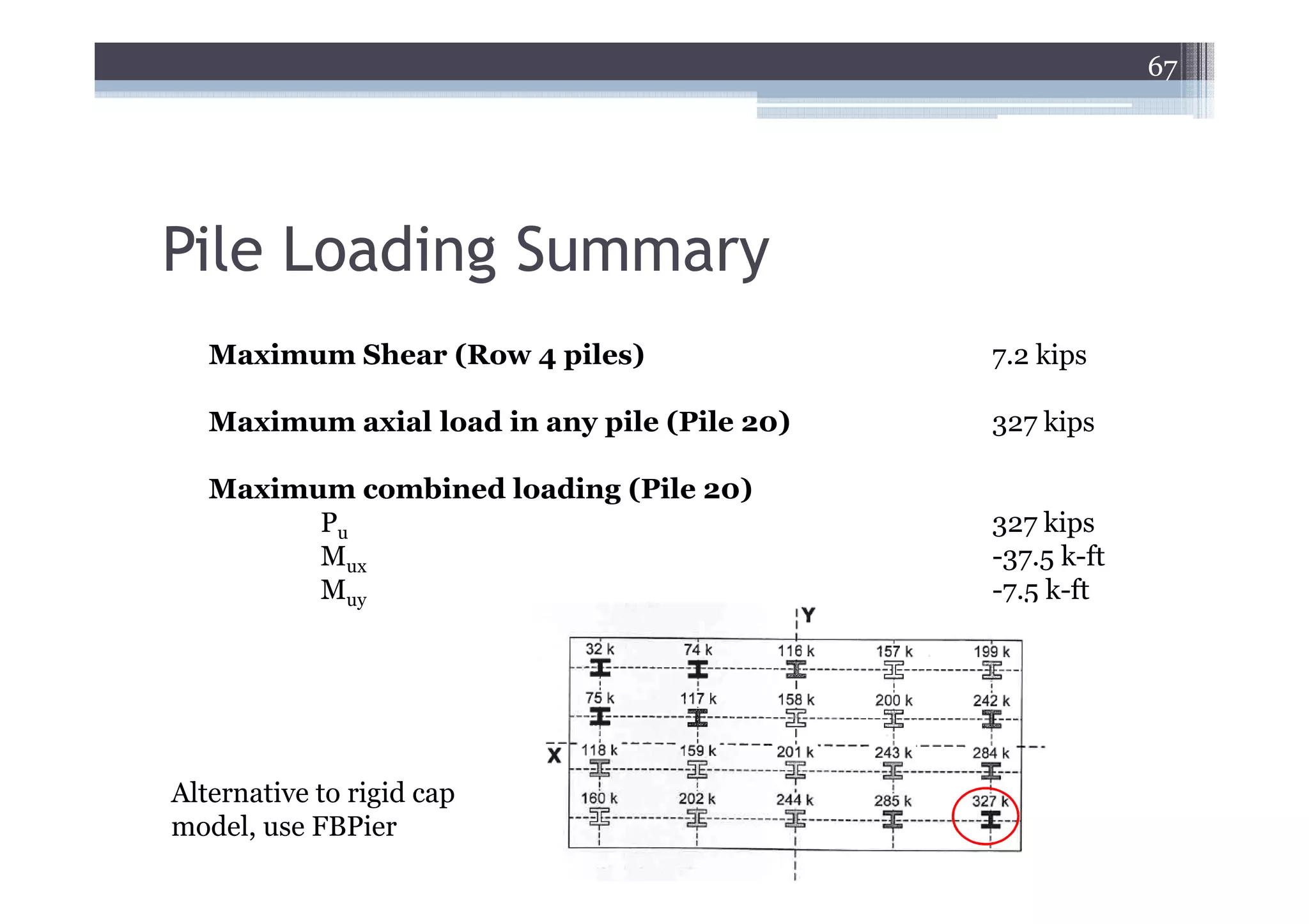
67
Pile Loading Summary
Maximum Shear (Row 4 piles) 7.2 kips
Maximum axial load in any pile (Pile 20) 327 kips
Maximum combined loading (Pile 20)
Pu 327 kips
Mux -37.5 k-ft
Muy -7.5 k-ft
Alternative to rigid cap
model, use FBPier
68.
68
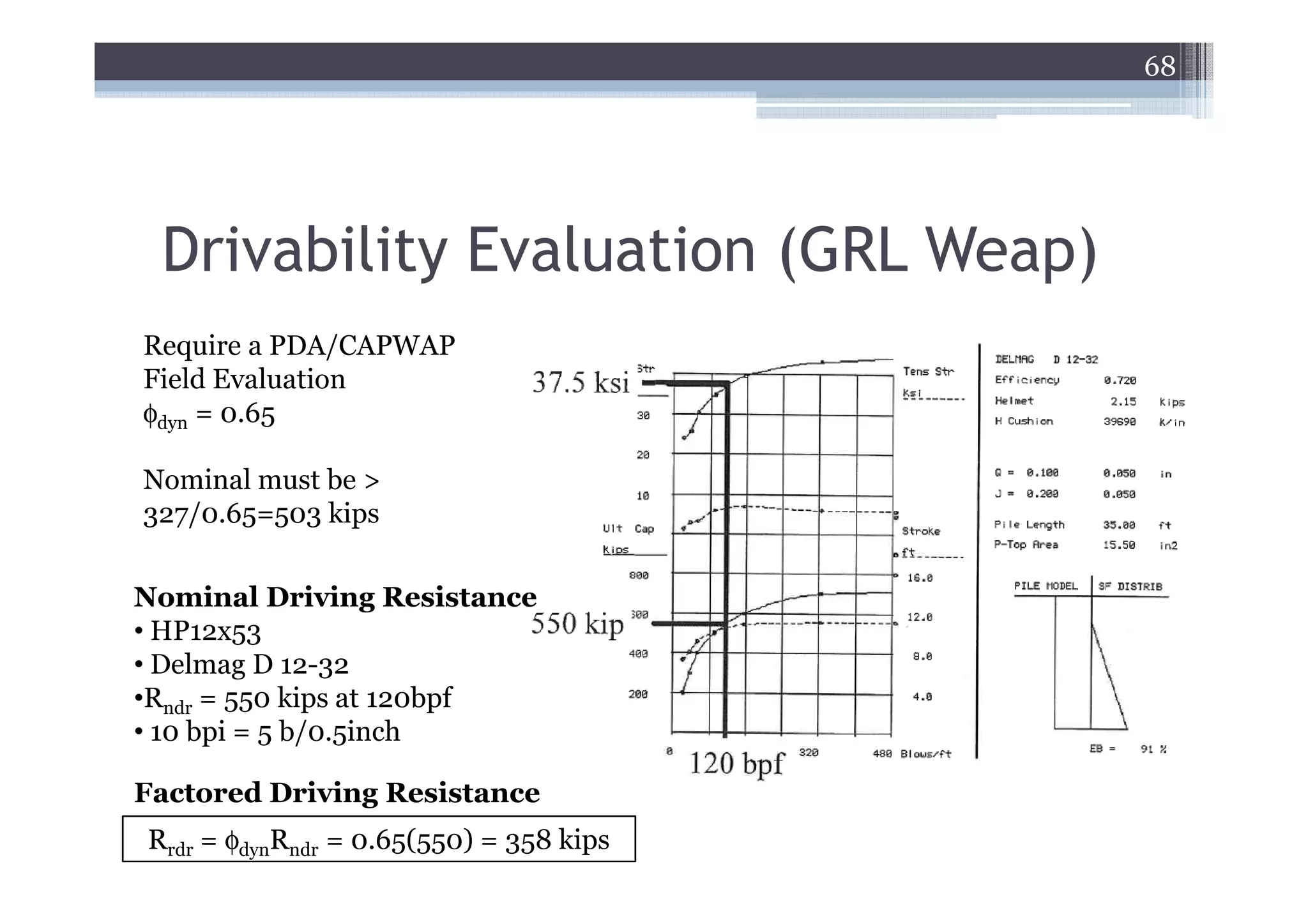
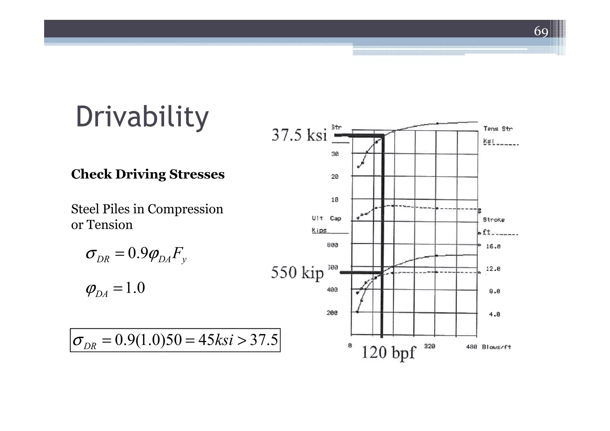
Drivability Evaluation(GRL Weap)
Require a PDA/CAPWAP
Field Evaluation
φdyn = 0.65
Nominal must be >
327/0.65=503 kips
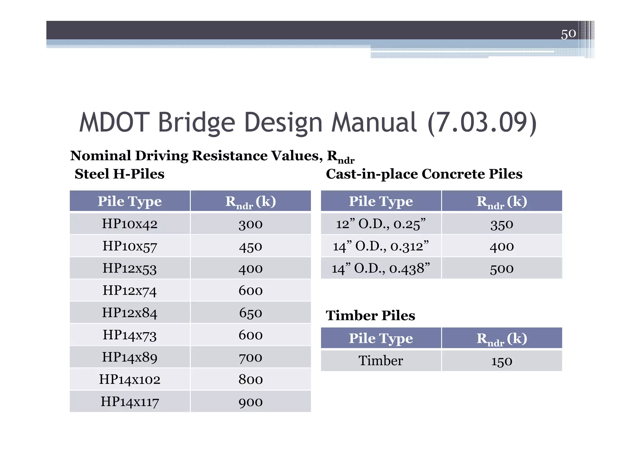
Nominal Driving Resistance
• HP12x53
• Delmag D 12-32
•Rndr = 550 kips at 120bpf
• 10 bpi = 5 b/0.5inch
Factored Driving Resistance
Rrdr = φdynRndr = 0.65(550) = 358 kips
70
Geotechnical Resistance -Static
Estimate the Depth of Penetration φdyn Rn = 358kips = φstat Rnstat
Use SPT method φ = 0.3
Rnstat = 358/0.3 = 1193 kips !!!
Very long piles would be required if all loose sand!! For our geology, the
piles would end bear on till or bedrock and develop full capacity within a
few feet of penetration (usual for H-piles). End bearing on rock (φ =
0.45). Pile tips required and driving resistance and criteria will be based
on dynamic testing in the field (PDA/CAPWAP).
71.
71
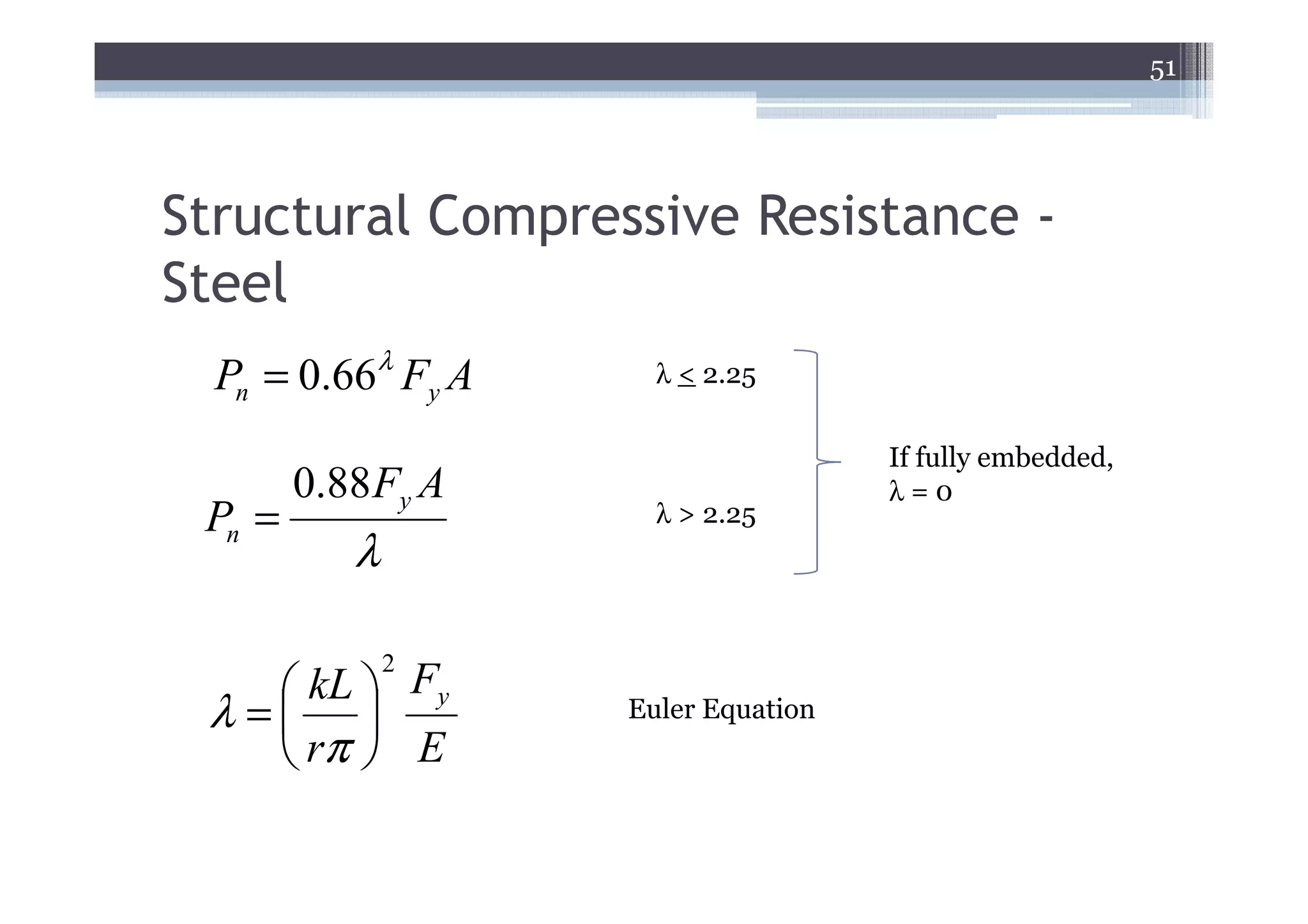
Structural Resistance -Compression
Nominal Compressive Resistance (Section 6.9.4.1)
Pn = 0.66λ Fy A Compression only, damage likely
φ = 0.5
λ =0 Fully embedded
Compression only, damage unlikely
Pn = Fy A = 50(15.5) = 775kips φ = 0.6
Combined
Factored Compressive Resistance φ = 0.7
Pr = φPn = 0.5(775) = 387.5kips
Good for lower portion of pile where damage is more likely
Pr = φPn = 0.7(775) = 542.5kips combined
72.
72
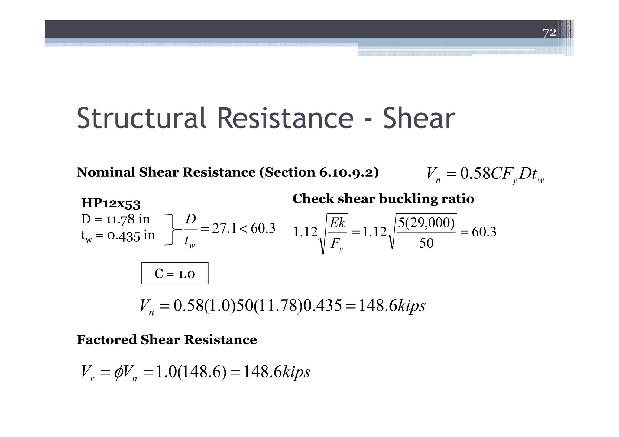
Structural Resistance -Shear
Nominal Shear Resistance (Section 6.10.9.2) Vn = 0.58CFy Dt w
HP12x53 Check shear buckling ratio
D = 11.78 in D Ek 5(29,000)
tw = 0.435 in = 27.1 < 60.3 1.12 = 1.12 = 60.3
tw Fy 50
C = 1.0
Vn = 0.58(1.0)50(11.78)0.435 = 148.6kips
Factored Shear Resistance
Vr = φVn = 1.0(148.6) = 148.6kips
73.
73
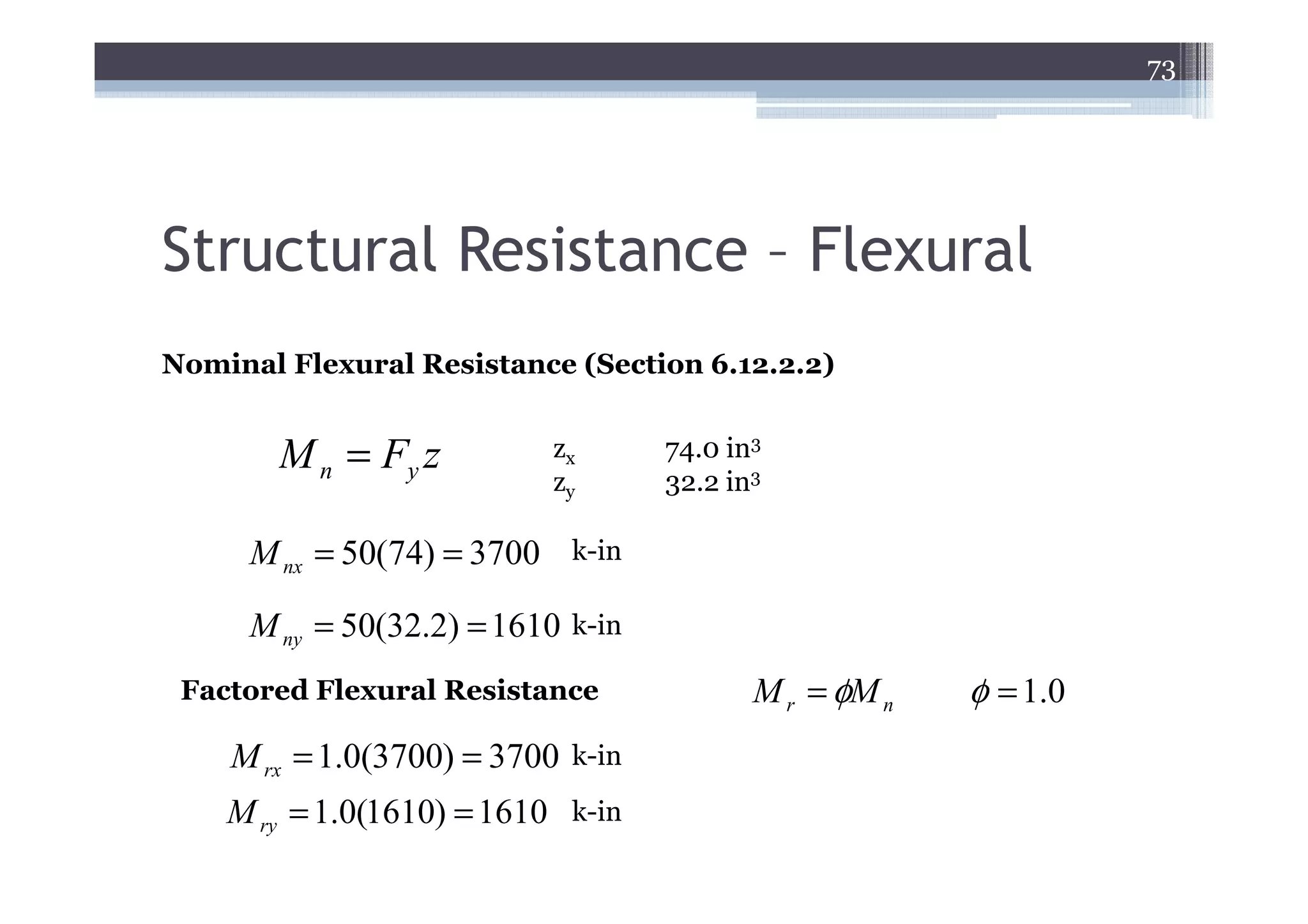
Structural Resistance –Flexural
Nominal Flexural Resistance (Section 6.12.2.2)
M n = Fy z zx 74.0 in3
zy 32.2 in3
M nx = 50(74) = 3700 k-in
M ny = 50(32.2) = 1610 k-in
Factored Flexural Resistance M r = φM n φ = 1.0
M rx = 1.0(3700) = 3700 k-in
M ry = 1.0(1610) = 1610 k-in
74.
74
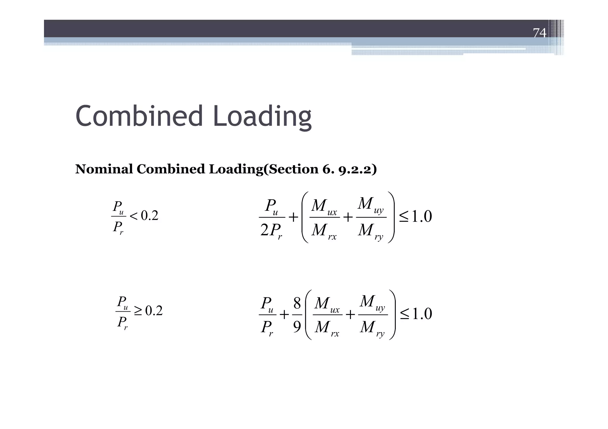
Combined Loading
Nominal CombinedLoading(Section 6. 9.2.2)
Pu Pu M ux M uy
< 0.2 + + ≤ 1.0
Pr 2 Pr M rx M ry
Pu Pu 8 M ux M uy
≥ 0.2 + + ≤ 1.0
Pr Pr 9 M rx M ry
75.
75
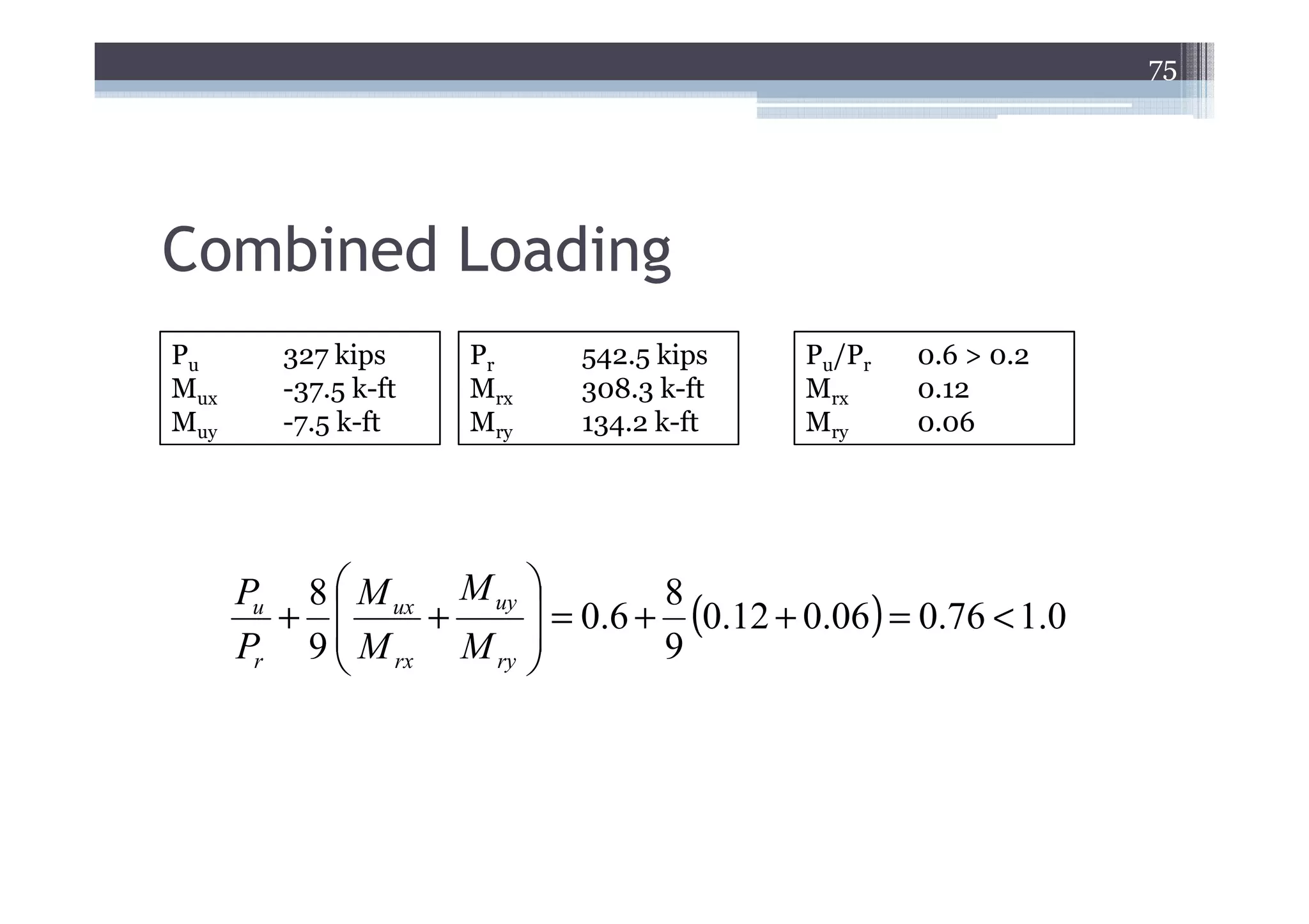
Combined Loading
Pu 327 kips Pr 542.5 kips Pu/Pr 0.6 > 0.2
Mux -37.5 k-ft Mrx 308.3 k-ft Mrx 0.12
Muy -7.5 k-ft Mry 134.2 k-ft Mry 0.06
Pu 8 M ux M uy
= 0.6 + 8 (0.12 + 0.06) = 0.76 < 1.0
+ +
Pr 9 rx M ry
M
9
76.
76
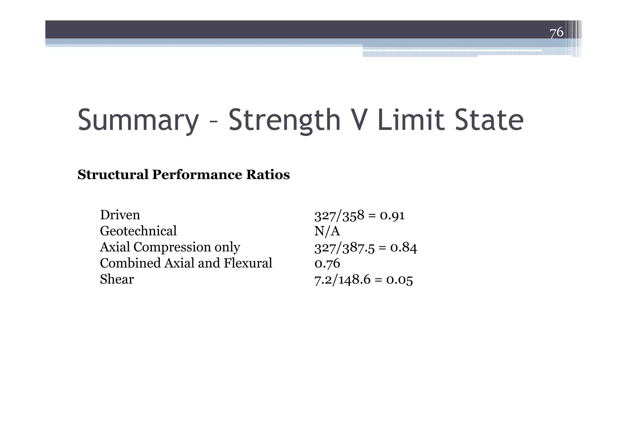
Summary – StrengthV Limit State
Structural Performance Ratios
Driven 327/358 = 0.91
Geotechnical N/A
Axial Compression only 327/387.5 = 0.84
Combined Axial and Flexural 0.76
Shear 7.2/148.6 = 0.05
82
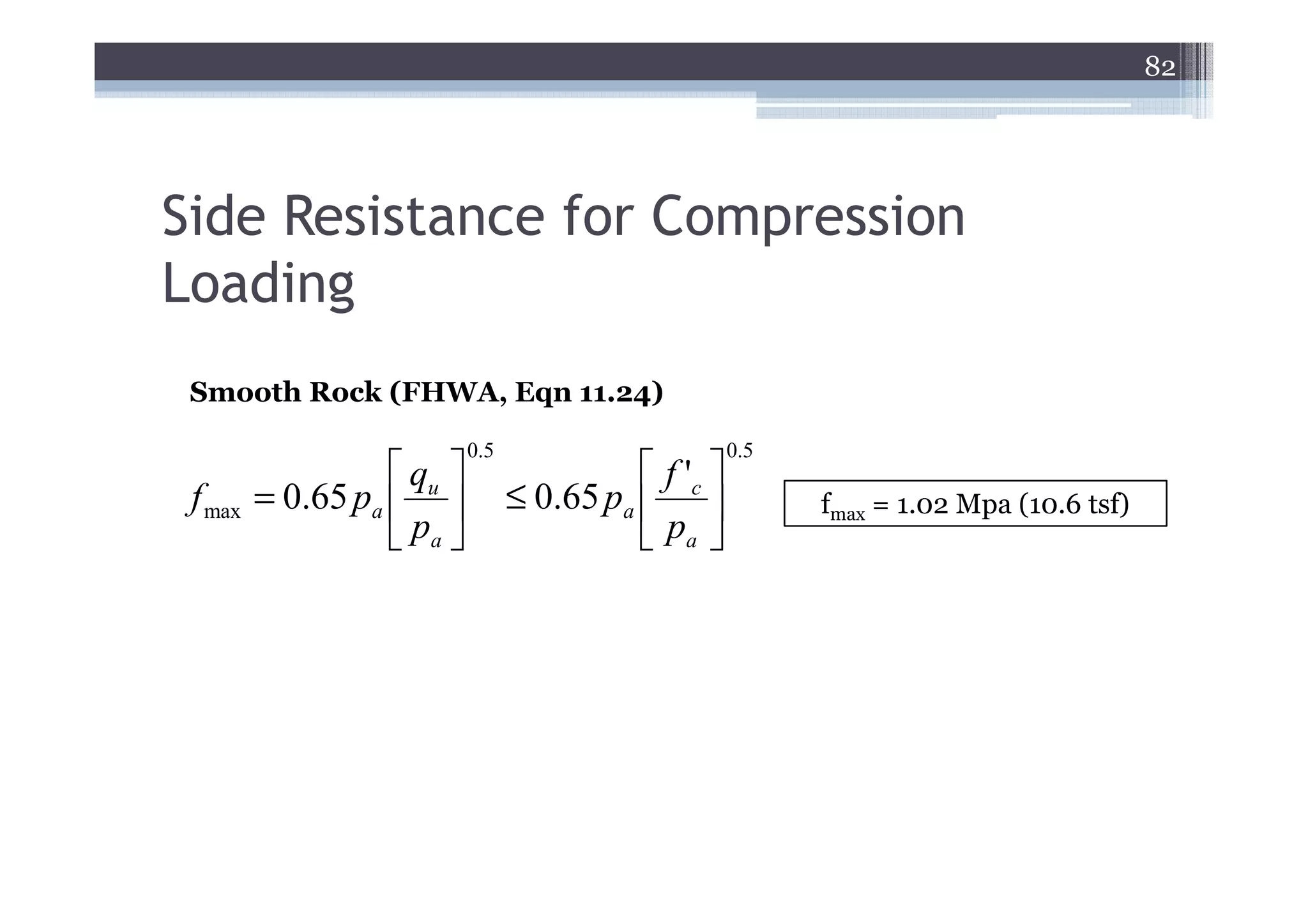
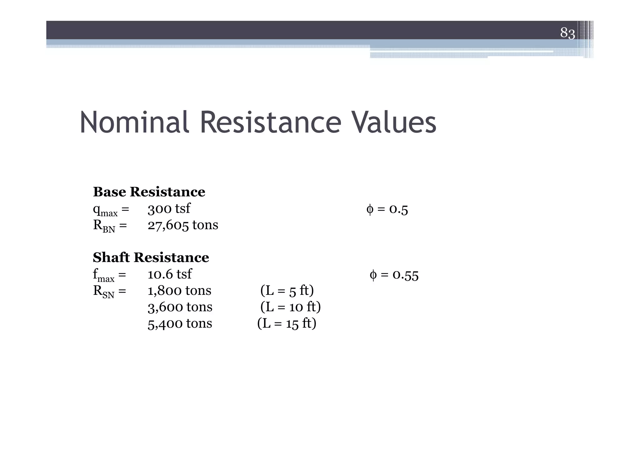
Side Resistance forCompression
Loading
Smooth Rock (FHWA, Eqn 11.24)
0.5 0.5
qu f 'c
f max = 0.65 pa ≤ 0.65 pa fmax = 1.02 Mpa (10.6 tsf)
pa pa
85
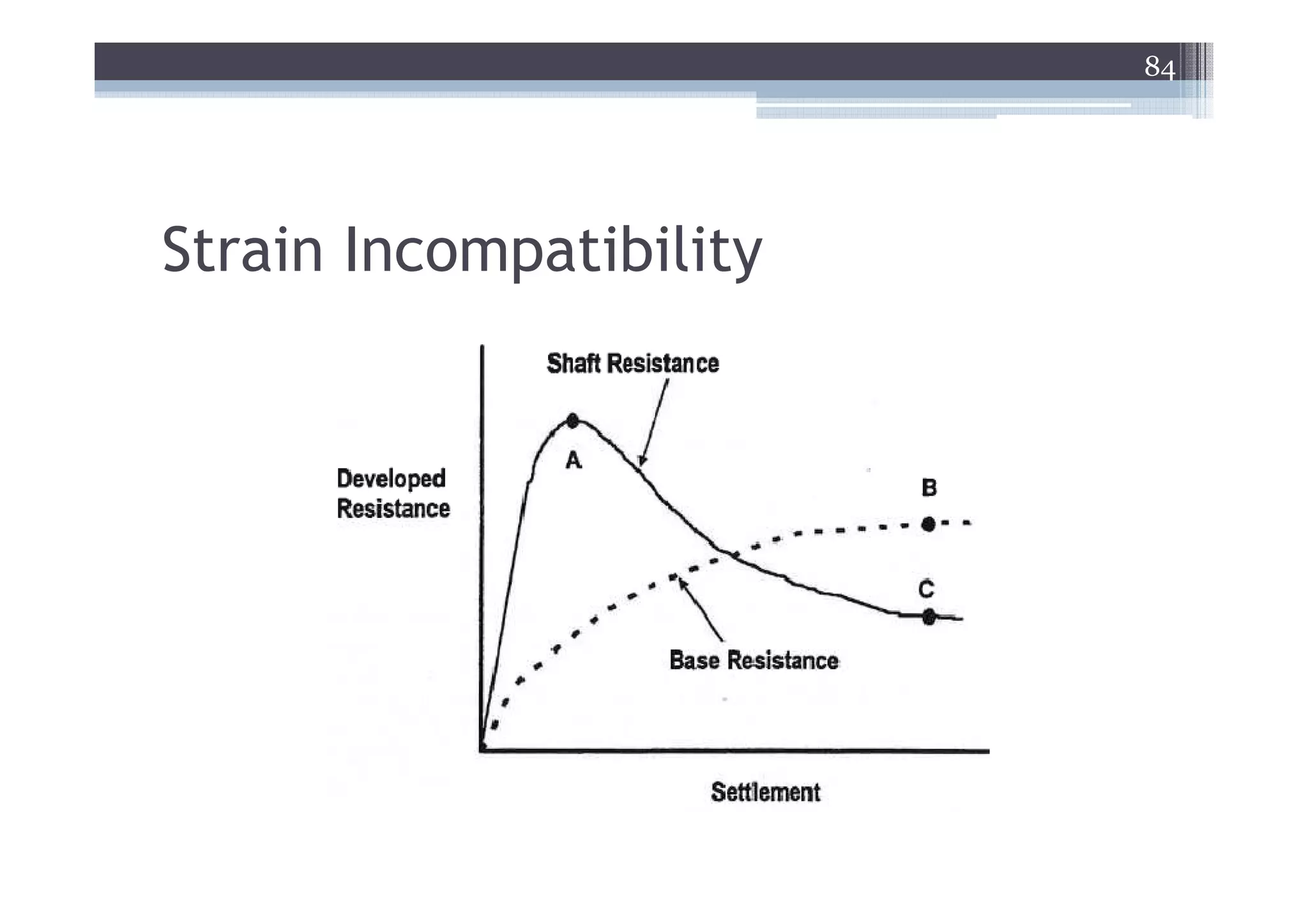
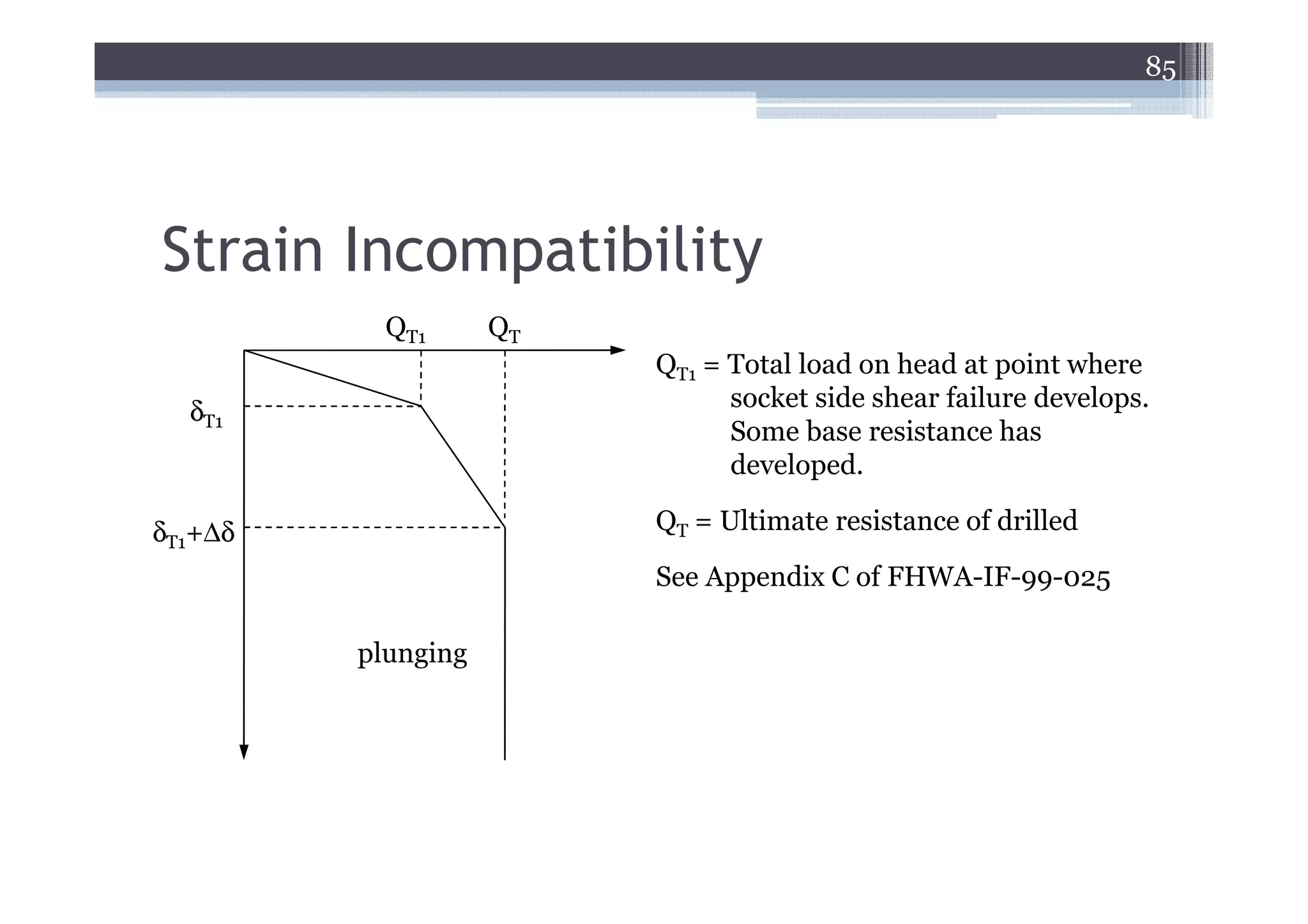
Strain Incompatibility
QT1 QT
QT1 = Total load on head at point where
δT1 socket side shear failure develops.
Some base resistance has
developed.
δT1+∆δ QT = Ultimate resistance of drilled
See Appendix C of FHWA-IF-99-025
plunging
![34
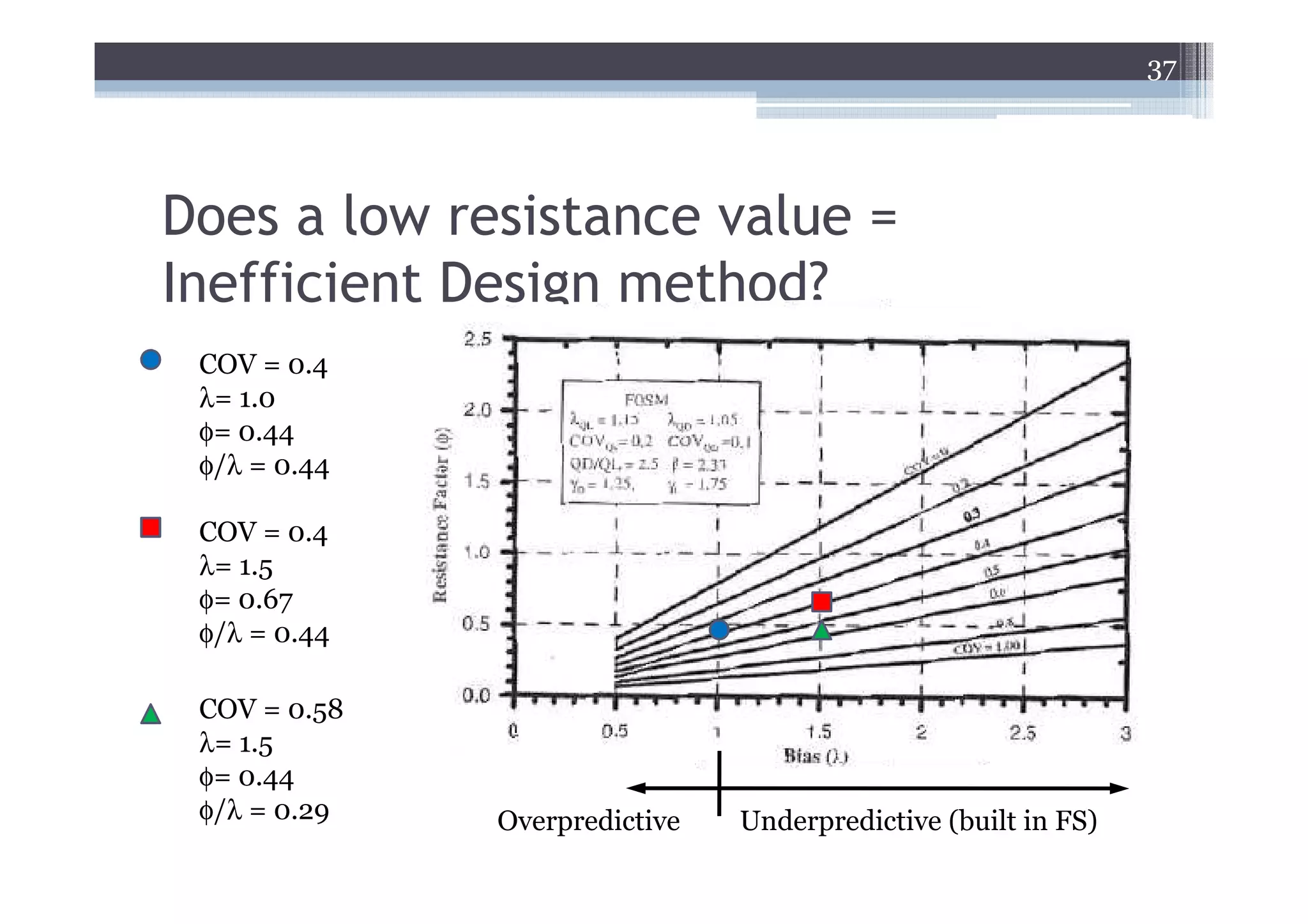
Resistance Factor
1 + COV Q
2
λR (Σγ i Qi )
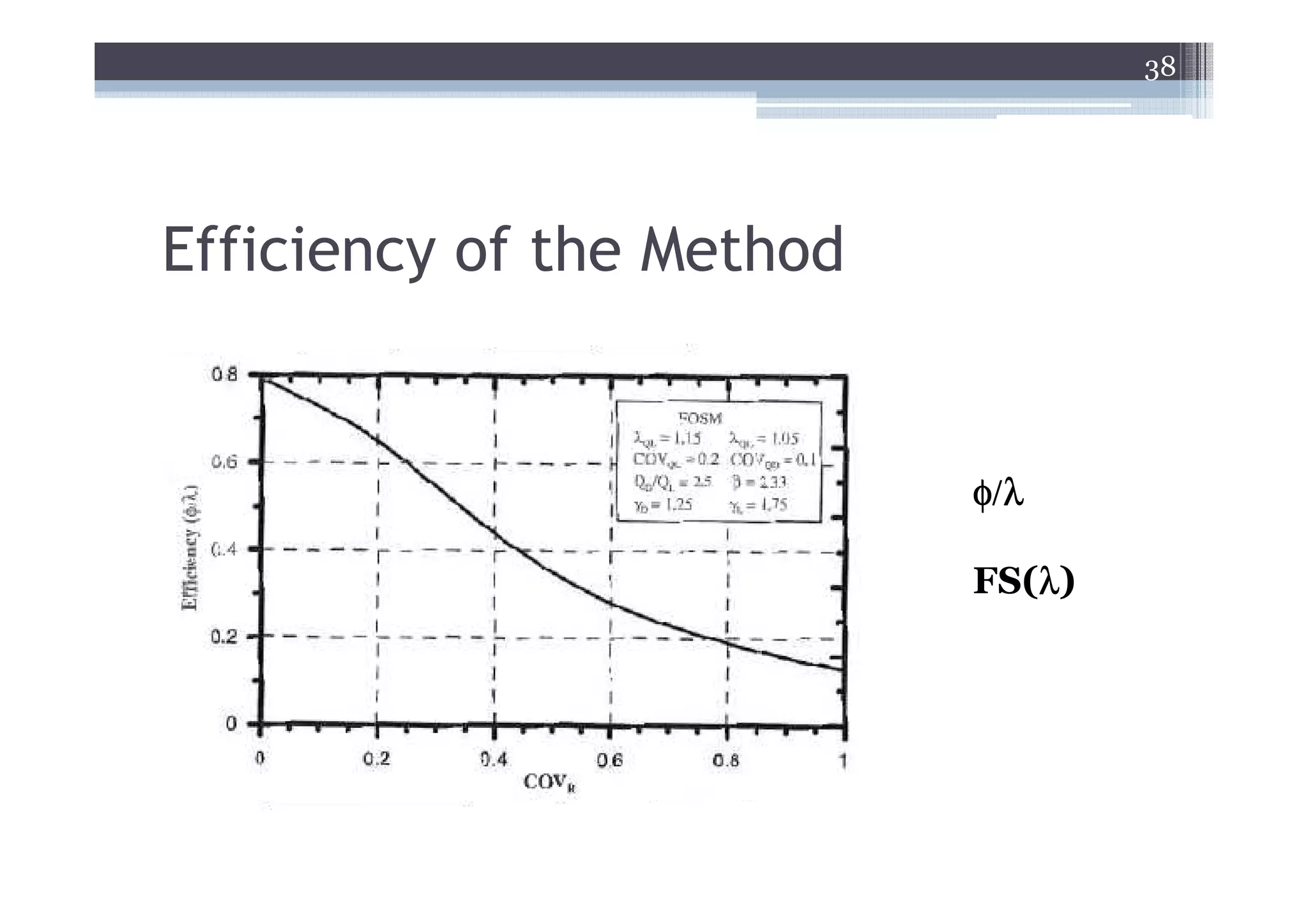
1 + COV R
2
φ=
{ [(
Q exp βT ln 1 + COVR 1 + COVQ
2
)( 2
)]}
Dead Load Factors
γD = 1.25
λQD = 1.05
COVQD = 0.1
QD
Live Load Factors γD +γL
γL = 1.75 QL 1.4167
λQL = 1.15
FS = ≅
QD φ
COVQL = 0.2 φ
+ 1
QL ](https://image.slidesharecdn.com/lrfdshortcoursepresentation-12526274988162-phpapp03/75/Lrfd-Short-Course-Presentation-34-2048.jpg)


![80
Base Resistance for Compressive
Loading
Rock with 70 < RQD < 100 (FHWA, Eqn 11.6)
qmax ( MPa) = 4.83[qu ( MPa)]
0.51
qmax = 44.9 Mpa (469 tsf)
[ ]q
Jointed Rock (FHWA, Eqn, 11.7)
0.5
(
qmax = s + ms + s0.5
)
0.5
u
qmax = 49.5 Mpa (517 tsf)
Detroit Experience
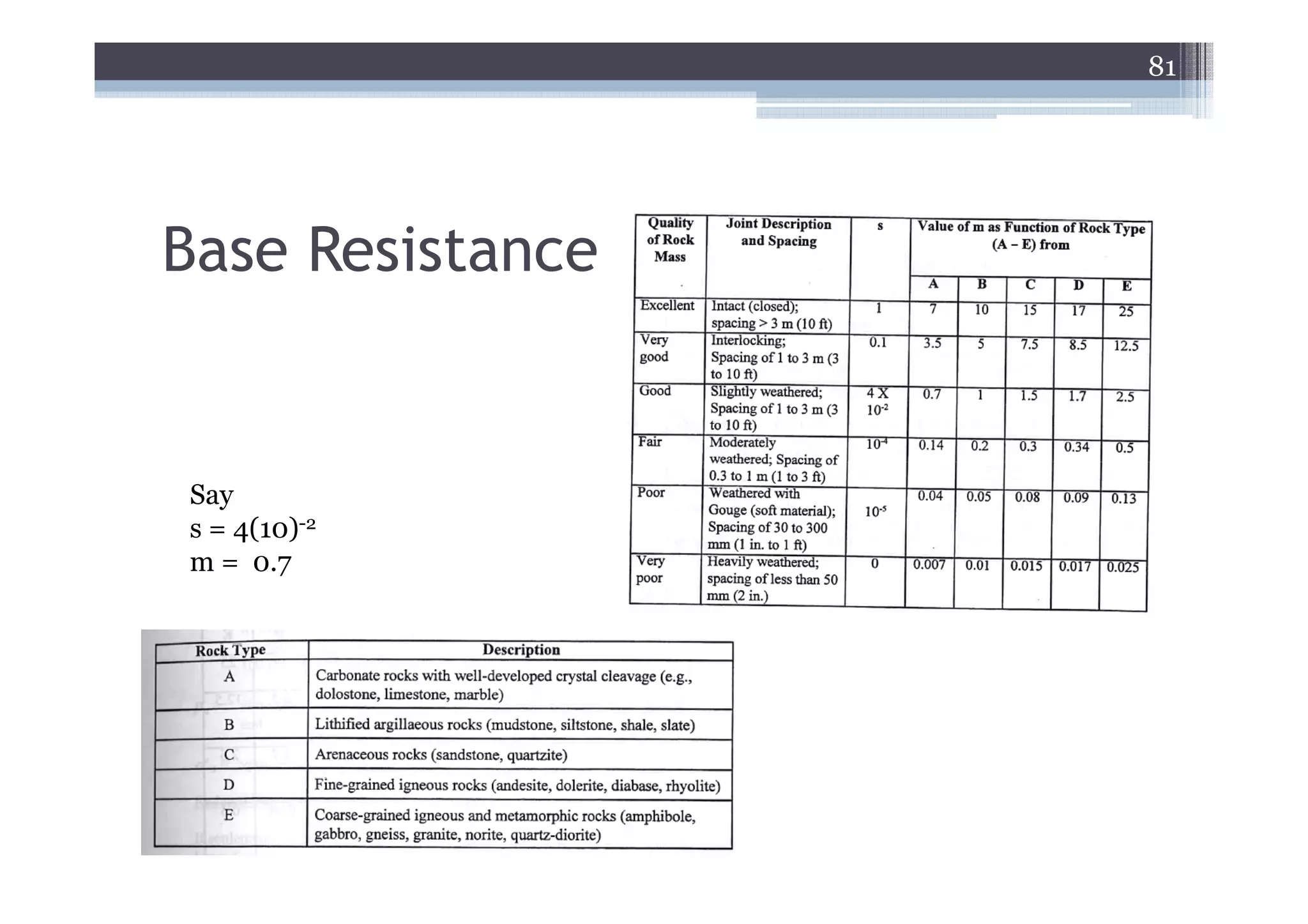
qmax = qall (FS ) = 120(2.5) qmax = 28.7Mpa (300 tsf)](https://image.slidesharecdn.com/lrfdshortcoursepresentation-12526274988162-phpapp03/75/Lrfd-Short-Course-Presentation-80-2048.jpg)


![[프레스세미나 1주제] 16년도 프레스업종 세미나 자료](https://cdn.slidesharecdn.com/ss_thumbnails/116-160518004446-thumbnail.jpg?width=640&height=640&fit=bounds)


