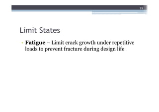
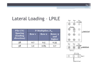
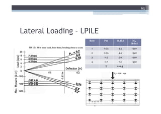
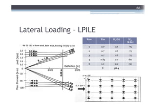
This document provides an overview of Load and Resistance Factor Design (LRFD) for deep foundations, with a focus on:
1. The differences between Allowable Stress Design (ASD) and LRFD approaches.
2. Key concepts in LRFD including limit states, load factors, load combinations, resistance factors, reliability, and efficiency of design methods.
3. How LRFD approaches are applied specifically to deep foundation design, including the use of limit states for service, strength, and extreme load conditions according to the AASHTO Bridge Design Specifications.

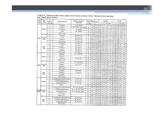
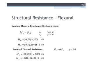
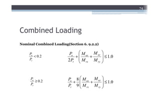
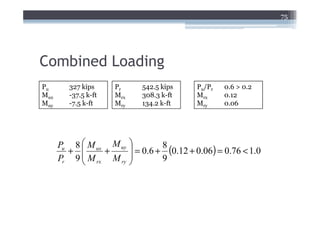
![34
Resistance Factor
1 + COV Q
2
λR (Σγ i Qi )
1 + COV R
2
φ=
{ [(
Q exp βT ln 1 + COVR 1 + COVQ
2
)( 2
)]}
Dead Load Factors
γD = 1.25
λQD = 1.05
COVQD = 0.1
QD
Live Load Factors γD +γL
γL = 1.75 QL 1.4167
λQL = 1.15
FS = ≅
QD φ
COVQL = 0.2 φ
+ 1
QL ](https://image.slidesharecdn.com/lrfdshortcoursepresentation-12526274988162-phpapp03/85/Lrfd-Short-Course-Presentation-34-320.jpg)
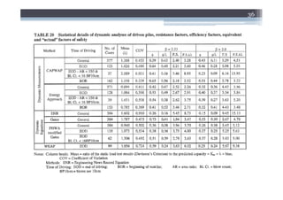


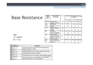
![80
Base Resistance for Compressive
Loading
Rock with 70 < RQD < 100 (FHWA, Eqn 11.6)
qmax ( MPa) = 4.83[qu ( MPa)]
0.51
qmax = 44.9 Mpa (469 tsf)
[ ]q
Jointed Rock (FHWA, Eqn, 11.7)
0.5
(
qmax = s + ms + s0.5
)
0.5
u
qmax = 49.5 Mpa (517 tsf)
Detroit Experience
qmax = qall (FS ) = 120(2.5) qmax = 28.7Mpa (300 tsf)](https://image.slidesharecdn.com/lrfdshortcoursepresentation-12526274988162-phpapp03/85/Lrfd-Short-Course-Presentation-80-320.jpg)


![[프레스세미나 1주제] 16년도 프레스업종 세미나 자료](https://cdn.slidesharecdn.com/ss_thumbnails/116-160518004446-thumbnail.jpg?width=640&height=640&fit=bounds)


