Downloaded 435 times
![ 1
N = initial oil in place ( STB ) = Vφ (1 − S wc ) ( STB )
Boi
initial H .C. Vol. of the gascap SCF ft 3 bbl
m= (= const.) [=] or or
initial H .C. Vol. of the oil SCF ft 3 bbl
N p = cumulative oil production (STB )
cum. gas production ( SCF )
R p = cumulative gas − oil rato =
cum. oil production ( STB )](https://image.slidesharecdn.com/2009chapter4materialbalance-130119005036-phpapp01/75/Material-balance-Equation-3-2048.jpg)
![Expansion of oil & originally dissolved gas
Liquid exp ansion (oil exp ansion) = liq. (at p ) − liq. (at pi )
RB
= NBo − NBoi = N ( Bo − Boi )[=]STB [=]RB (3.1)
STB
Liberated gas exp ansion = − [ solution gas (at p) − solution gas (at pi )]
SCF RB
= NRsi B g − NRs B g = N ( Rsi − Rs ) B g [=]STB [=]RB (3.2)
STB SCF](https://image.slidesharecdn.com/2009chapter4materialbalance-130119005036-phpapp01/75/Material-balance-Equation-4-2048.jpg)
![Expansion of the gascap gas
Expansion of the gascap gas =gascap gas (at p) –gascap (at pi)
SCF RB
The total volume of gascap gas = mNBoi [=] STB [=]RB
SCF SCF
1 1
or G = mNBoi [=]RB [=]SCF
B gi RB
SCF
1 RB
Amount of gas (at p ) = mNBoi B g [=]SCF [=]RB
B gi SCF
Bg
Expansion of the gascap gas = mNBoi − mNBoi [ =]RB
B gi
Bg
= mNBoi ( − 1) ( RB) (3.3)
B gi](https://image.slidesharecdn.com/2009chapter4materialbalance-130119005036-phpapp01/75/Material-balance-Equation-5-2048.jpg)
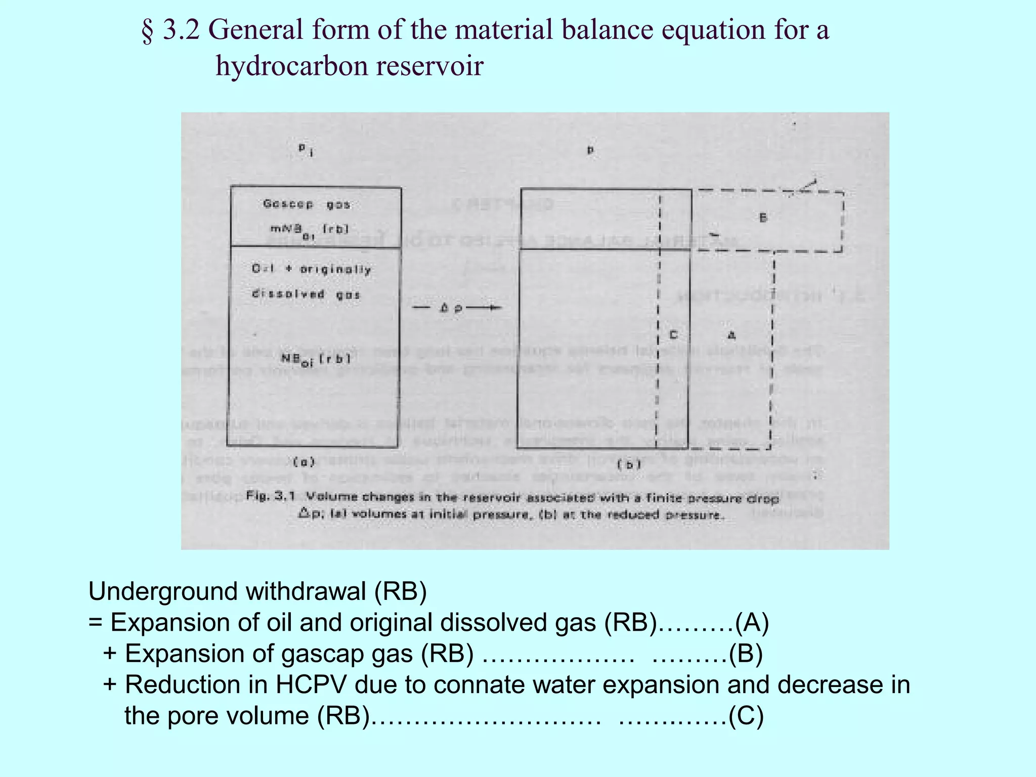
![Underground withdrawal
Pr oduction at surface N p ( STB ) − oil N p R p ( SCF ) − gas
Underground withdrawal N p Bo ( RB) − oil ( N p R p − N p Rs ) B g ( RB) − gas
⇒ Underground withdrawal = N p Bo + N p ( R p − Rs ) B g = N p [ Bo + ( R p − Rs ) B g ]](https://image.slidesharecdn.com/2009chapter4materialbalance-130119005036-phpapp01/75/Material-balance-Equation-7-2048.jpg)
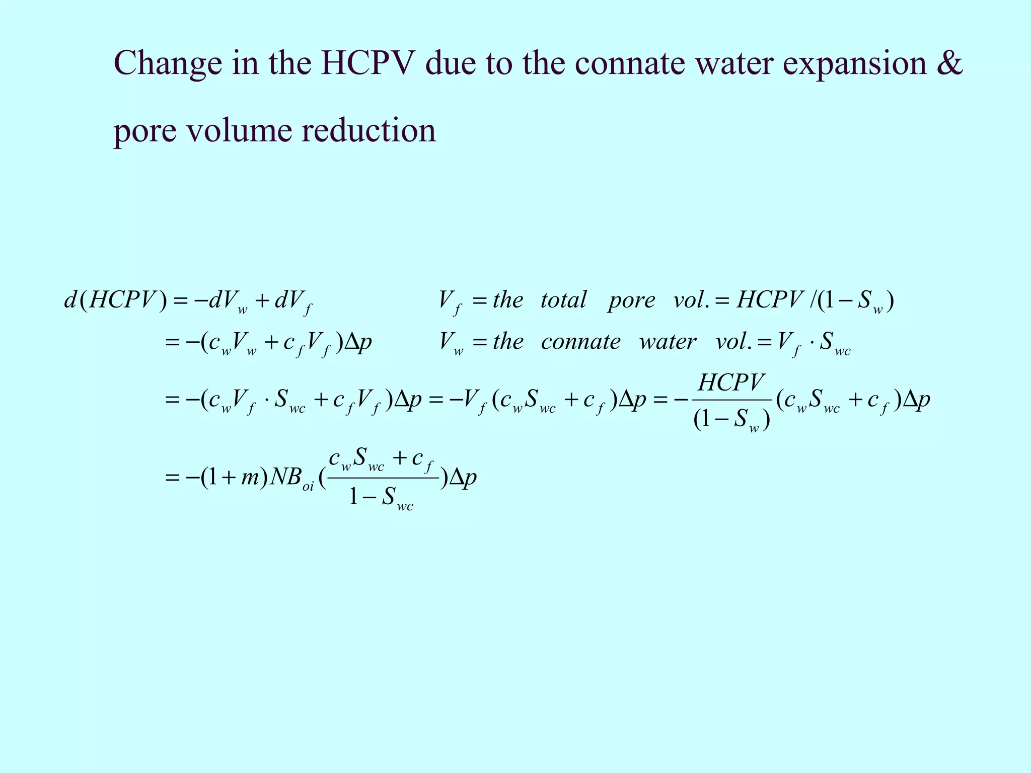
![The general expression for the material balance as
Bg
N p [ Bo + ( R p − Rs ) B g ] = N ( Bo − Boi ) + N ( Rsi − Rs ) B g + mNBoi ( − 1)
B gi
c w S wc + c f
+ (1 + m) NBoi ( )∆p + (We − W p ) Bw
1 − S wc
( Bo − Boi ) + ( Rsi − Rs ) B g Bg c w S wc + c f
⇒ N p [ Bo + ( R p − Rs ) B g ] = NBoi + m − 1 + (1 + m)
1− S ∆ p
Boi B
gi wc
+ (We − W p ) Bw (3.7)
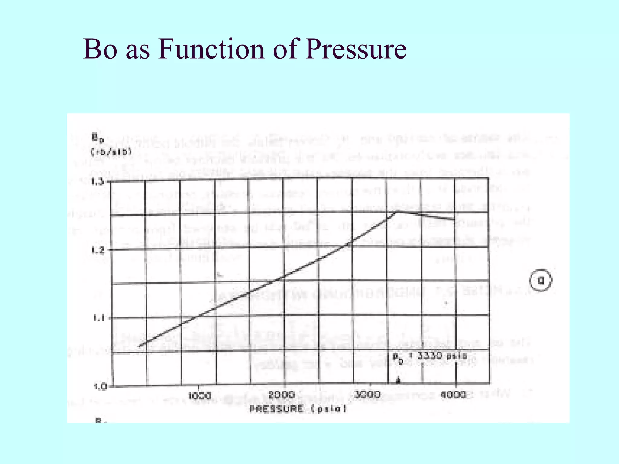
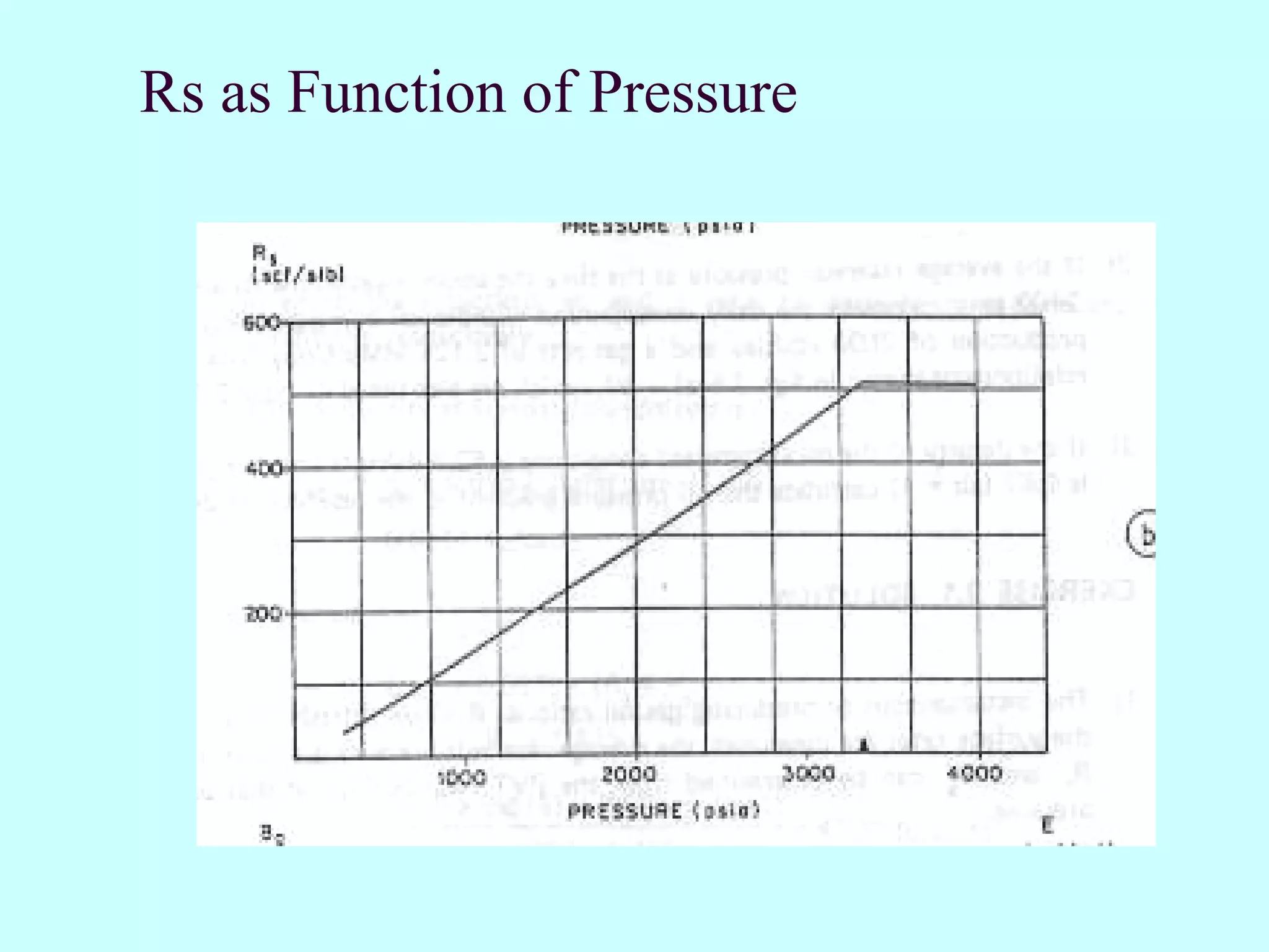
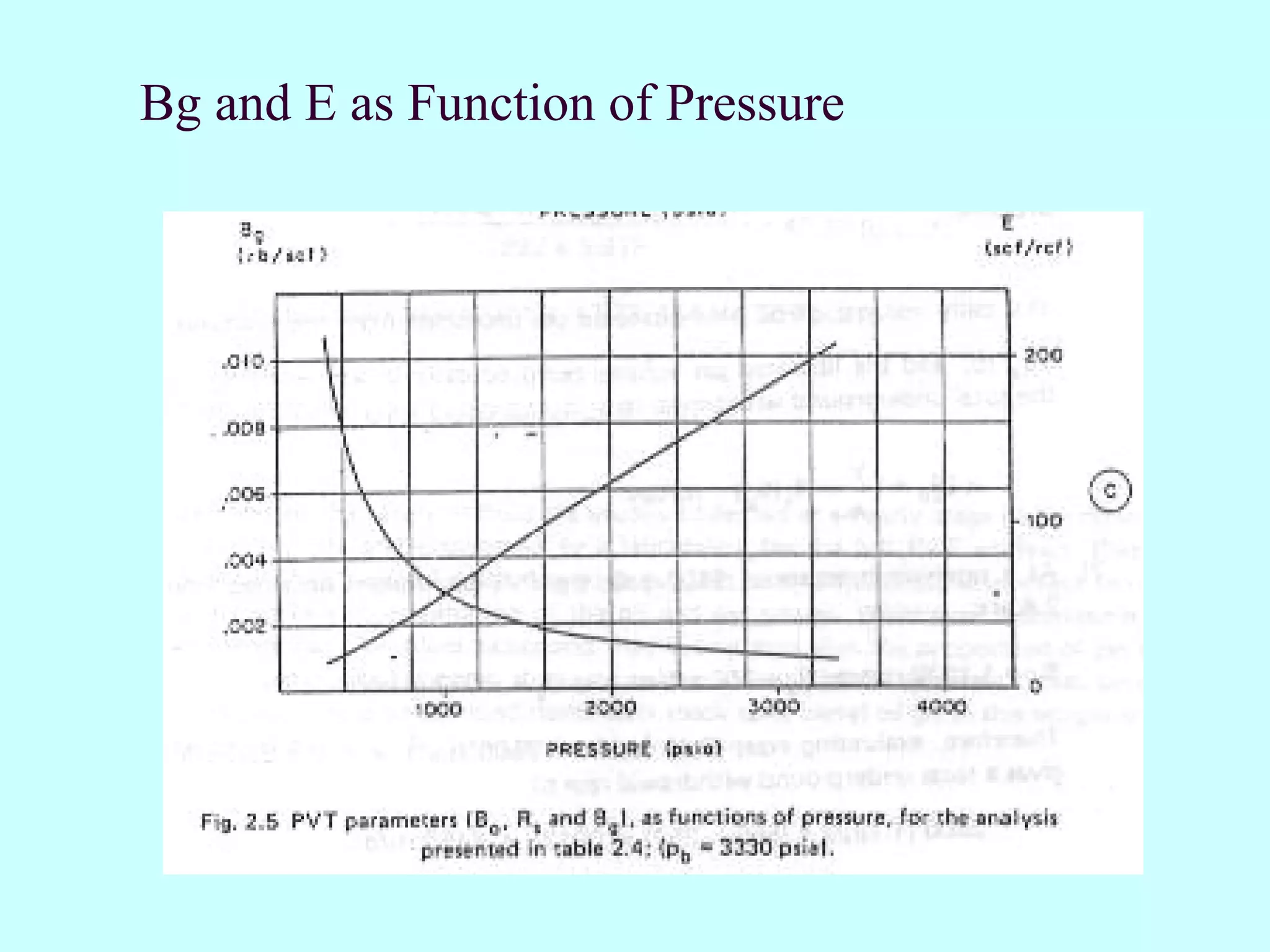
Note : Bo , Rs , B g = f ( p)
We = f ( p, t )
Simple form : Pr oduction = Expansion of reservoir fluids
dV = c ⋅ V ⋅ ∆p
Main difficulty : measuring p](https://image.slidesharecdn.com/2009chapter4materialbalance-130119005036-phpapp01/75/Material-balance-Equation-8-2048.jpg)
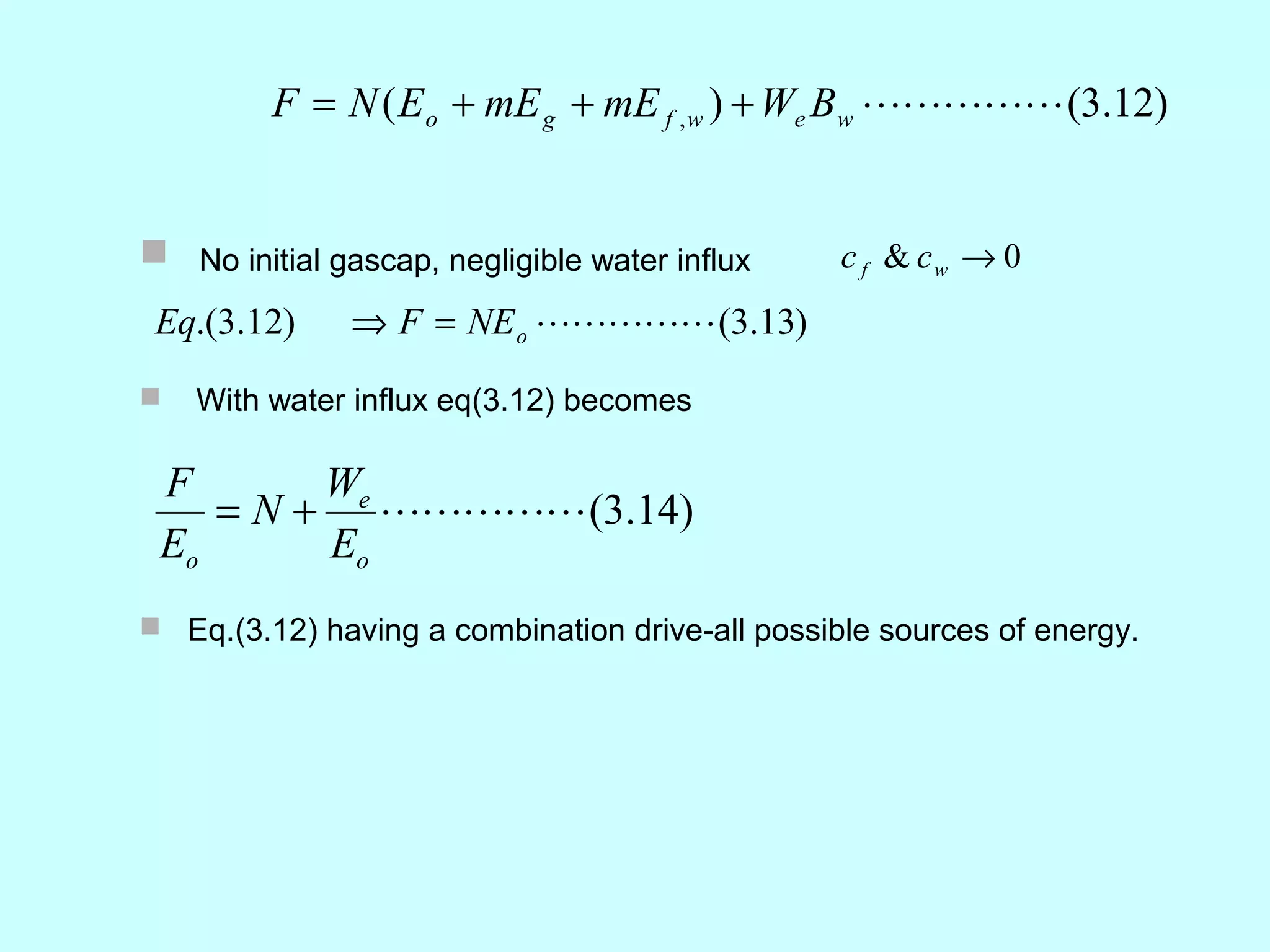
![F = N ( Eo + mE g + mE f ,w ) + We Bw (3.12)
where
F = N p [ Bo + ( R p − R s ) B g ] + W p B w [=]RB
E o = ( Bo − Boi ) + ( Rsi − Rs ) B g [=] RB
STB
Bg
E g = Boi ( − 1) [=] RB
B gi STB
c w S wc + c f
E f , w = (1 + m) Boi ( )∆p RB
1 − S wc STB](https://image.slidesharecdn.com/2009chapter4materialbalance-130119005036-phpapp01/75/Material-balance-Equation-9-2048.jpg)
![Above the B.P. pressure
- no initial gascap, m=0
- no water flux, We=0 ; no water production, Wp=0
- Rs=Rsi=Rp
from eq.(3.7)
( Bo − Boi ) + ( R si − R s ) B g Bg c w S wc + c f
N p [ Bo + ( R p − R s ) B g ] = NBoi + m − 1 + (1 + m)
1− S
∆p
Boi B
gi wc
+ (We − W p ) B w (3.7)
Note : ( R p − Rs ) = 0 ; ( Rsi − Rs ) = 0 ; m = 0 ;We = 0 ;W p = 0
( Bo − Boi ) (c w s wc + c f )
⇒ N p Bo = NBoi [ + ∆p ]
Boi 1 − S wc
cw S w + c f 1 dVo 1 dBo
⇒ N p Bo = NBoi [co + ( )]∆p co = − =−
1 − S wc Vo dp Bo dp
co S o + c w S w + c f − ( Boi − Bo ) ( Bo − Boi )
⇒ N p Bo = NBoi ( )∆p (3.17) ≈ =
1 − S wc Boi ∆p Boi ∆p
or N p Bo = NBoi ce ∆p (3.18) S o + S wc = 1
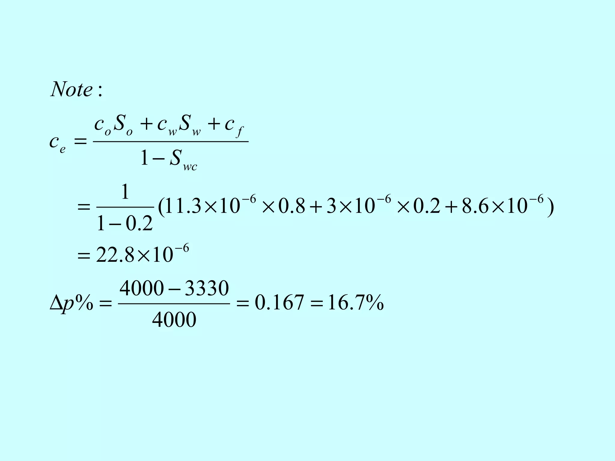
co S o + c w S w + c f
where ce = = the effective, saturation − weighted compressibility
1 − S wc](https://image.slidesharecdn.com/2009chapter4materialbalance-130119005036-phpapp01/75/Material-balance-Equation-13-2048.jpg)
![Exercise3.2 Solution gas drive; below bubble point pressure
Reservoir-described in exercise 3.1
Pabandon = 900psia
(1) R.F = f(Rp)? Conclusion?
(2) Sg(free gas) = F(Pabandon)?
Solution:
(1) From eq(3.7)
( Bo − Boi ) + ( R si − R s ) B g Bg c w S wc + c f
N p [ Bo + ( R p − Rs ) B g ] = NBoi + m − 1 + (1 + m)
1− S
∆ p
Boi B
gi wc
+ (We − W p ) B w (3.7)
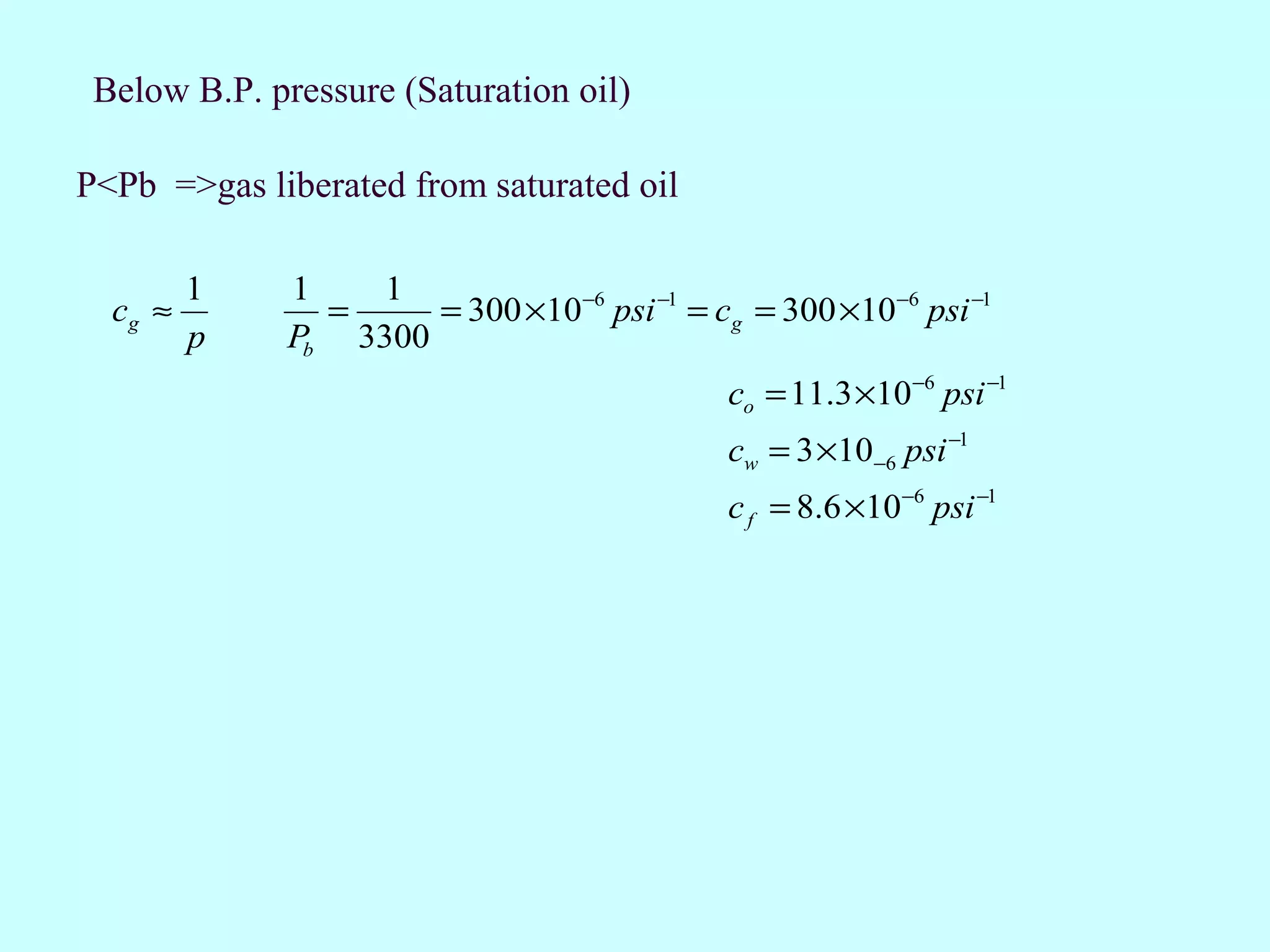
for solution gas below B.P.
−m =0 no initial gas cap
− We = 0 ; W p = 0
c w S wc + c f
− NBoi ( )∆p is negligible if S g is developed
1 − S wc](https://image.slidesharecdn.com/2009chapter4materialbalance-130119005036-phpapp01/75/Material-balance-Equation-22-2048.jpg)
![Eq(3.7) becomes
N p [ Bo + ( R p − Rs ) B g ] = N [( Bo − Boi ) + ( Rsi − Rs ) B g ] (3.20)
Np ( Bo − Boi ) + ( Rsi − Rs ) B g
R.F . = =
N Bo + ( R p − R s ) B g
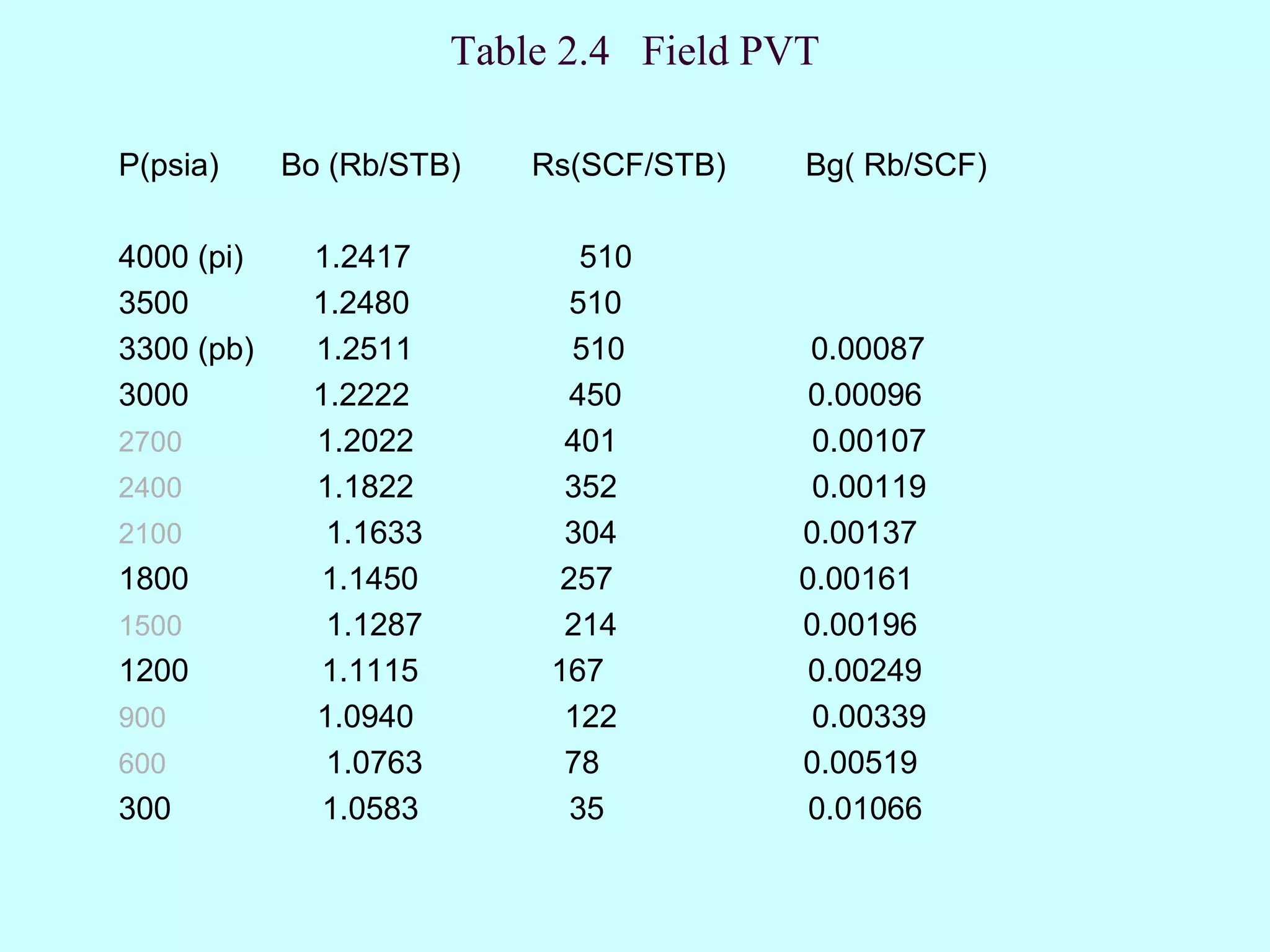
Np (1.0940 − 1.2417) + (510 − 122) × 0.00339 344
R.F . p =900 = = =
N p =900
1.0940 + ( R p − 122) × 0.00339 R p + 201
1
Conclusion: RF ≈
Rp
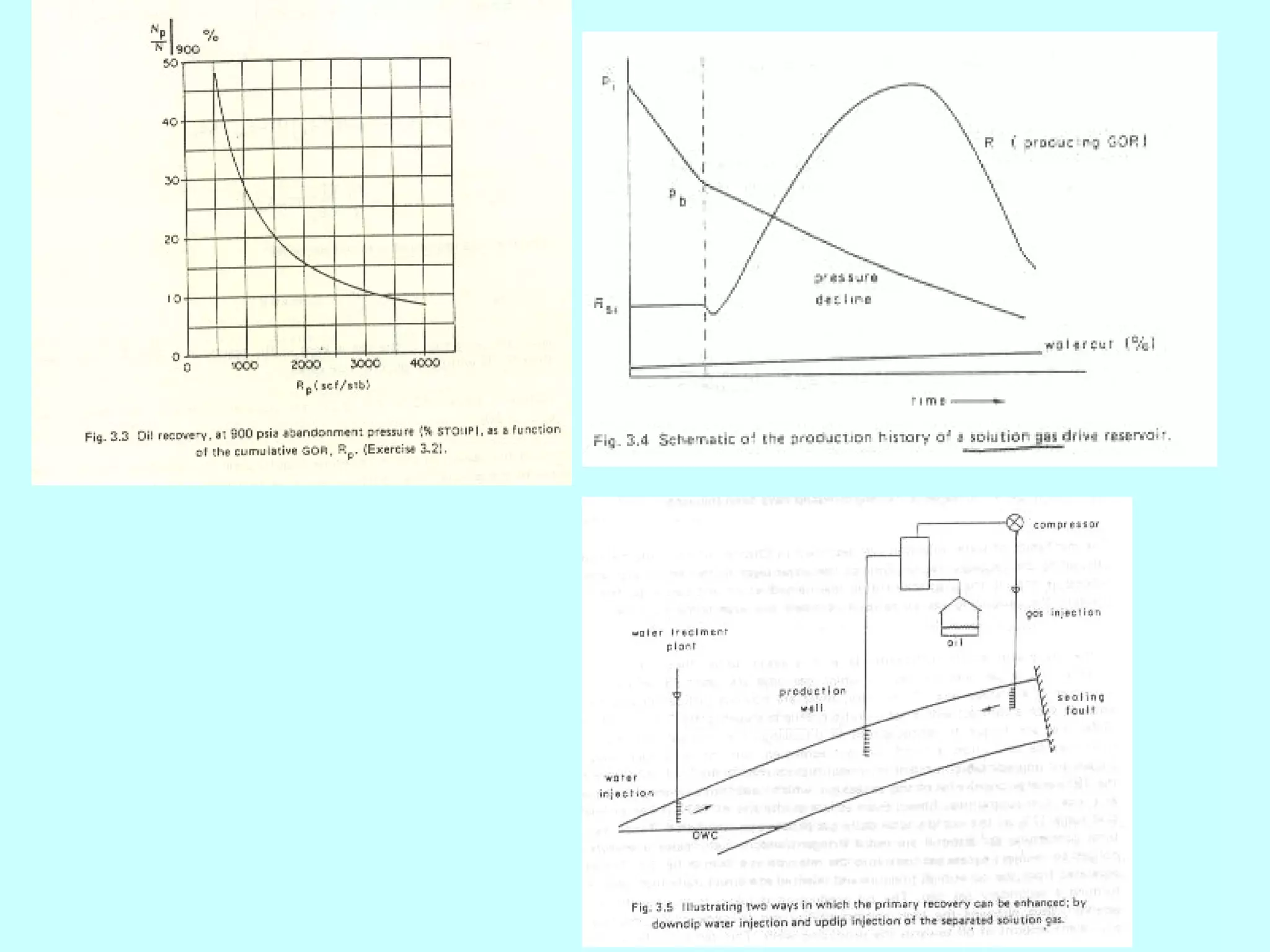
From Fig .3.3 ( p.55)
Np
R p = 500 SCF ⇒ = 49% = 0.49
STB N 900](https://image.slidesharecdn.com/2009chapter4materialbalance-130119005036-phpapp01/75/Material-balance-Equation-23-2048.jpg)
![(2) the overall gas balance
liberated total gas gas still
gas in the = amount −
− produced dissolved
reservoir of gas at surface in the oil
NBoi HCPV
= pore volume = for p > p b
1 − S wc (1 − S wc )
NBoi S g
⇒ = NR si B g − N p R p B g − ( N − N p ) Rs B g
(1 − S wc )
[ N ( Rsi − Rs ) − N p ( R p − Rs )]B g (1 − S wc )
⇒ Sg = (3.21)
NBoi
Np
[ N ( Rsi − Rs ) − Np( R p − Rs )]Bg (1 − S wc ) [( Rsi − Rs ) − ( R p − Rs )]
Sg = = N Bg (1 − S wc )
NBoi Boi
[(510 − 122) − 0.49(500 − 122)]
= × 0.00339 × 0.8 = 0.4428
1.2417](https://image.slidesharecdn.com/2009chapter4materialbalance-130119005036-phpapp01/75/Material-balance-Equation-25-2048.jpg)

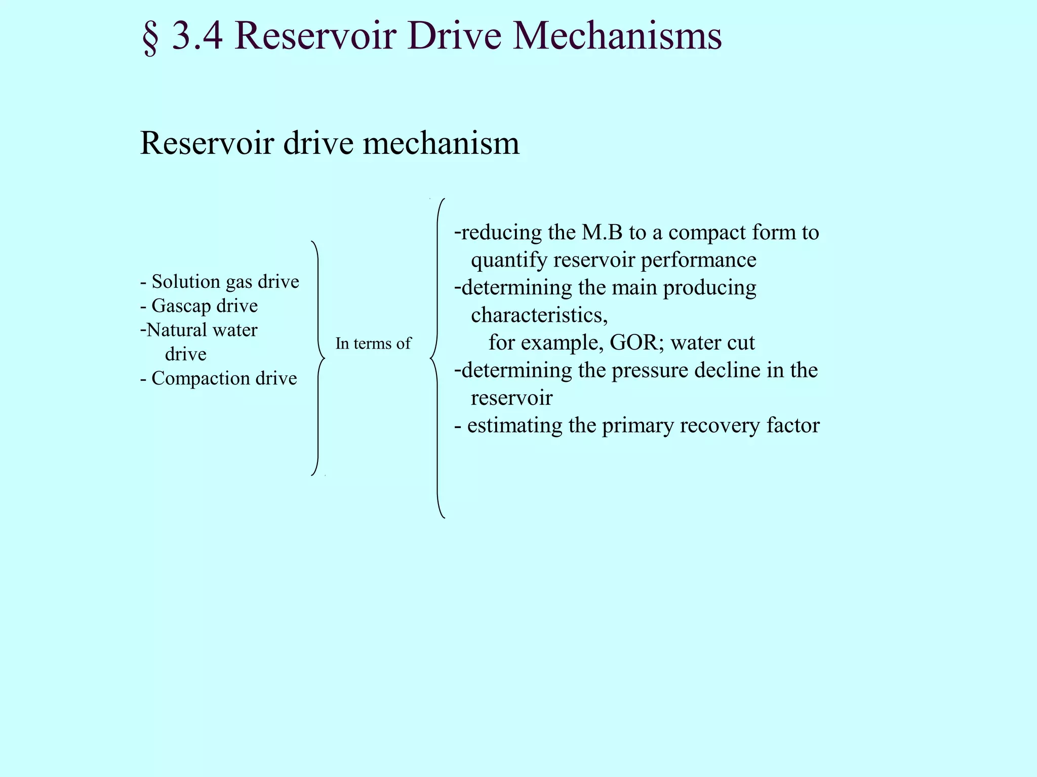
This document discusses material balance applied to oil reservoirs. It introduces the Schilthuis material balance equation, which is a basic tool for interpreting and predicting reservoir performance. The general form of the material balance equation accounts for underground withdrawal of oil and gas, expansion of oil and originally dissolved gas, expansion of any gas cap gas, and changes in hydrocarbon pore volume due to water and pore volume changes. The document provides the specific equations that make up the material balance and shows how it can be simplified for different reservoir drive mechanisms, including solution gas drive above and below the bubble point pressure. It also provides examples of calculating recovery factors and gas saturation from the material balance equation for a reservoir undergoing primary depletion by solution gas drive.