The document discusses the economic concept of demand. It defines the law of demand and explains the substitution and income effects that influence demand. It then discusses how individual consumer demand relates to market demand and how firm demand depends on market structure. Finally, it covers elasticity concepts including price elasticity of demand and its determinants.

2. Law of Demand Holding all other things constant ( ceteris paribus ), there is an inverse relationship between the price of a good and the quantity of the good demanded per time period. Substitution Effect Income Effect

3. Components of Demand: The Substitution Effect Assuming that real income is constant: If the relative price of a good rises, then consumers will try to substitute away from the good. Less will be purchased. If the relative price of a good falls, then consumers will try to substitute away from other goods. More will be purchased. The substitution effect is consistent with the law of demand.

4. Components of Demand: The Income Effect The real value of income is inversely related to the prices of goods. A change in the real value of income: will have a direct effect on quantity demanded if a good is normal. will have an inverse effect on quantity demanded if a good is inferior. The income effect is consistent with the law of demand only if a good is normal.

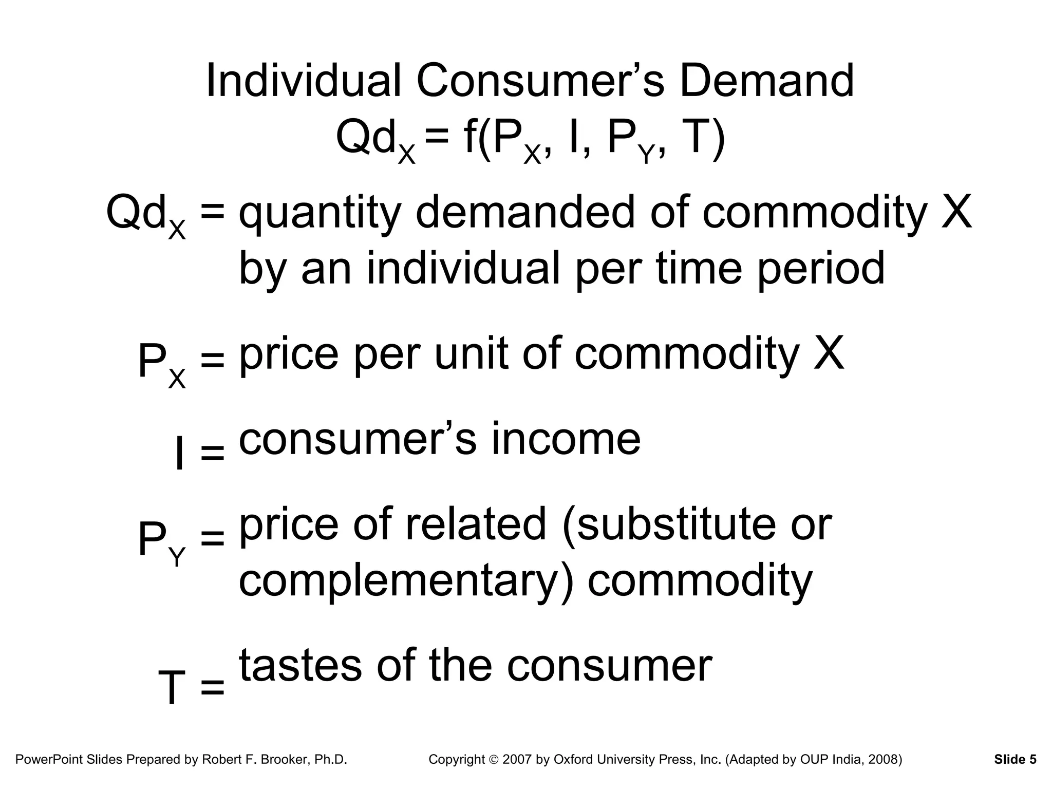
5. Individual Consumer’s Demand Qd X = f(P X , I, P Y , T) quantity demanded of commodity X by an individual per time period price per unit of commodity X consumer’s income price of related (substitute or complementary) commodity tastes of the consumer Qd X = P X = I = P Y = T =

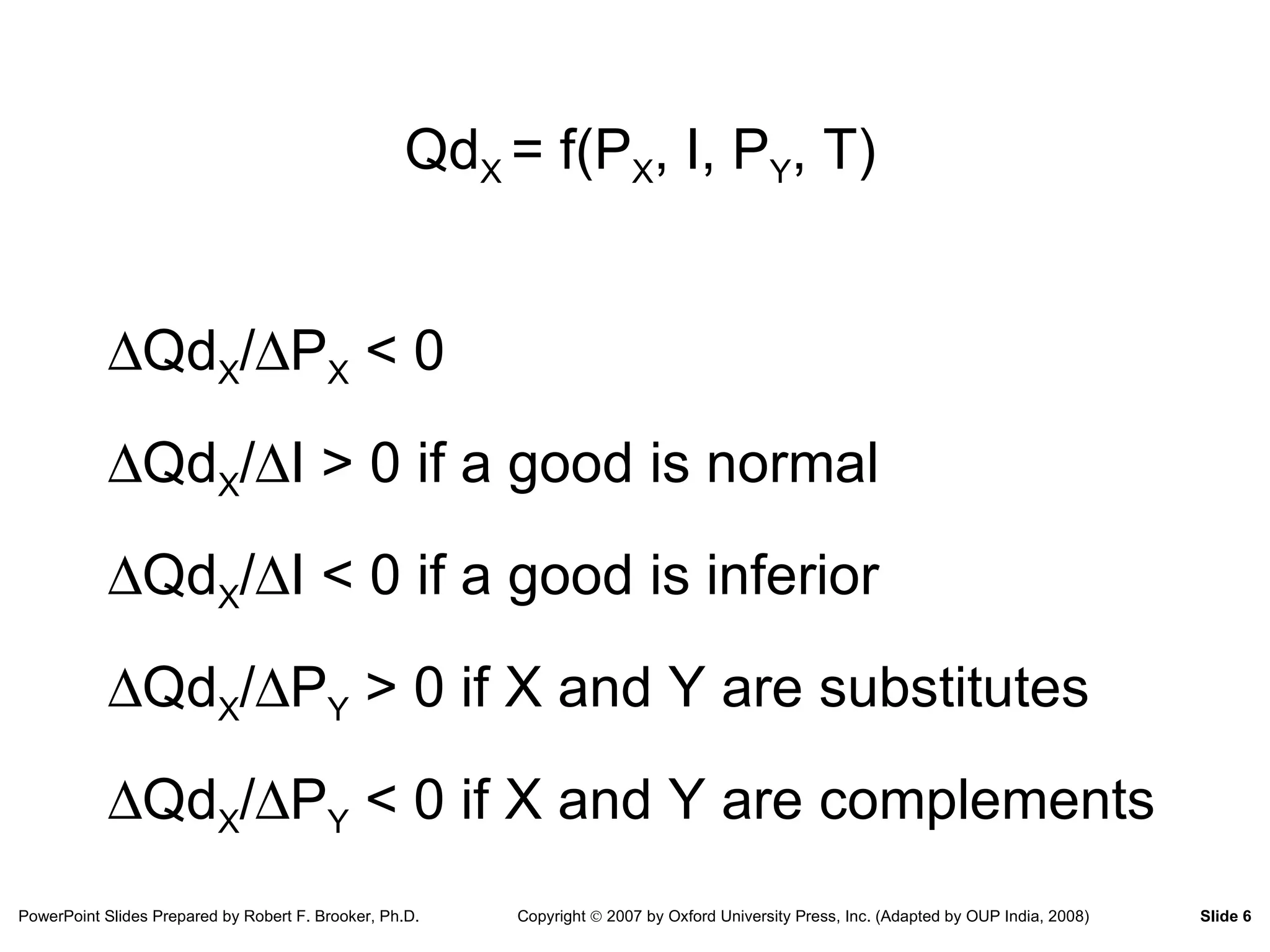
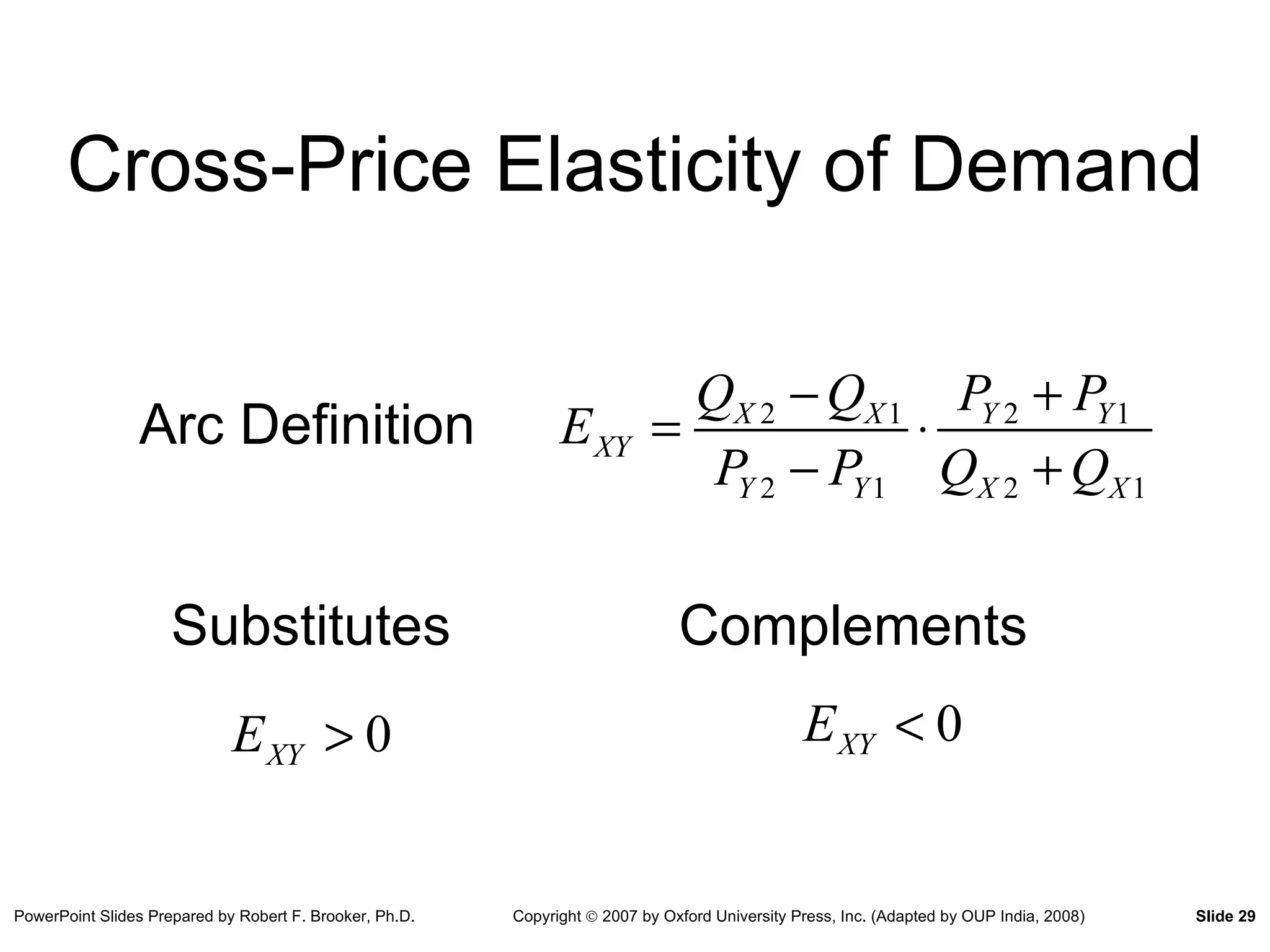
6. Qd X = f(P X , I, P Y , T)  Qd X /  P X < 0  Qd X /  I > 0 if a good is normal  Qd X /  I < 0 if a good is inferior  Qd X /  P Y > 0 if X and Y are substitutes  Qd X /  P Y < 0 if X and Y are complements

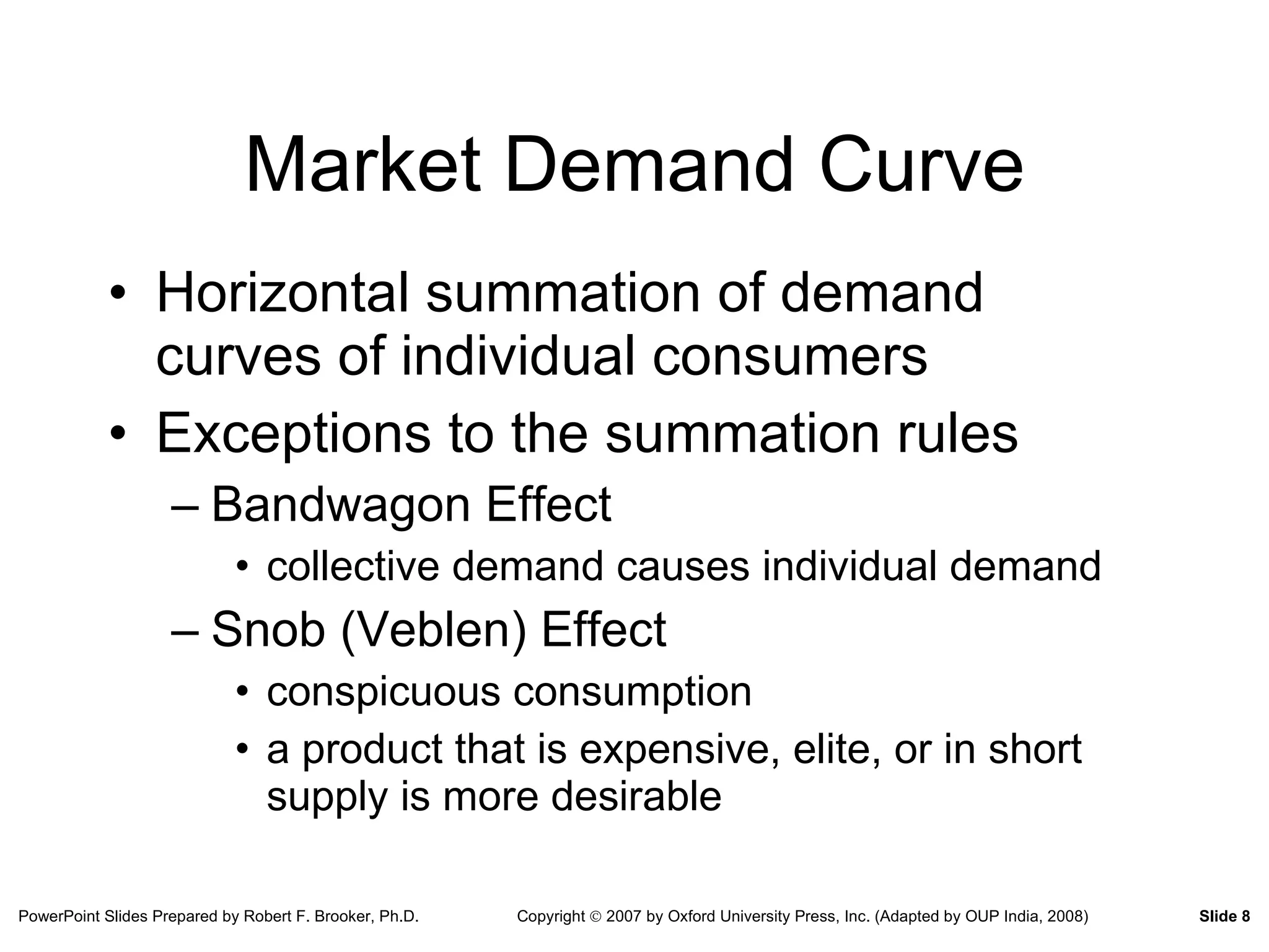
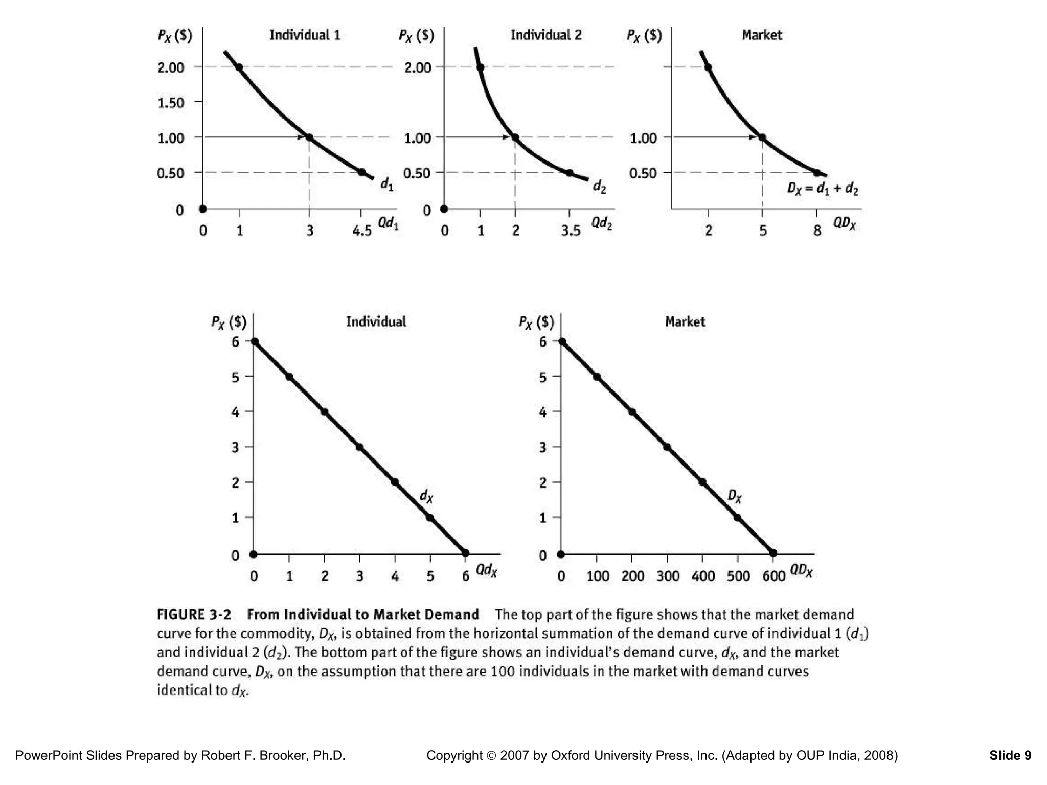
8. Market Demand Curve Horizontal summation of demand curves of individual consumers Exceptions to the summation rules Bandwagon Effect collective demand causes individual demand Snob (Veblen) Effect conspicuous consumption a product that is expensive, elite, or in short supply is more desirable

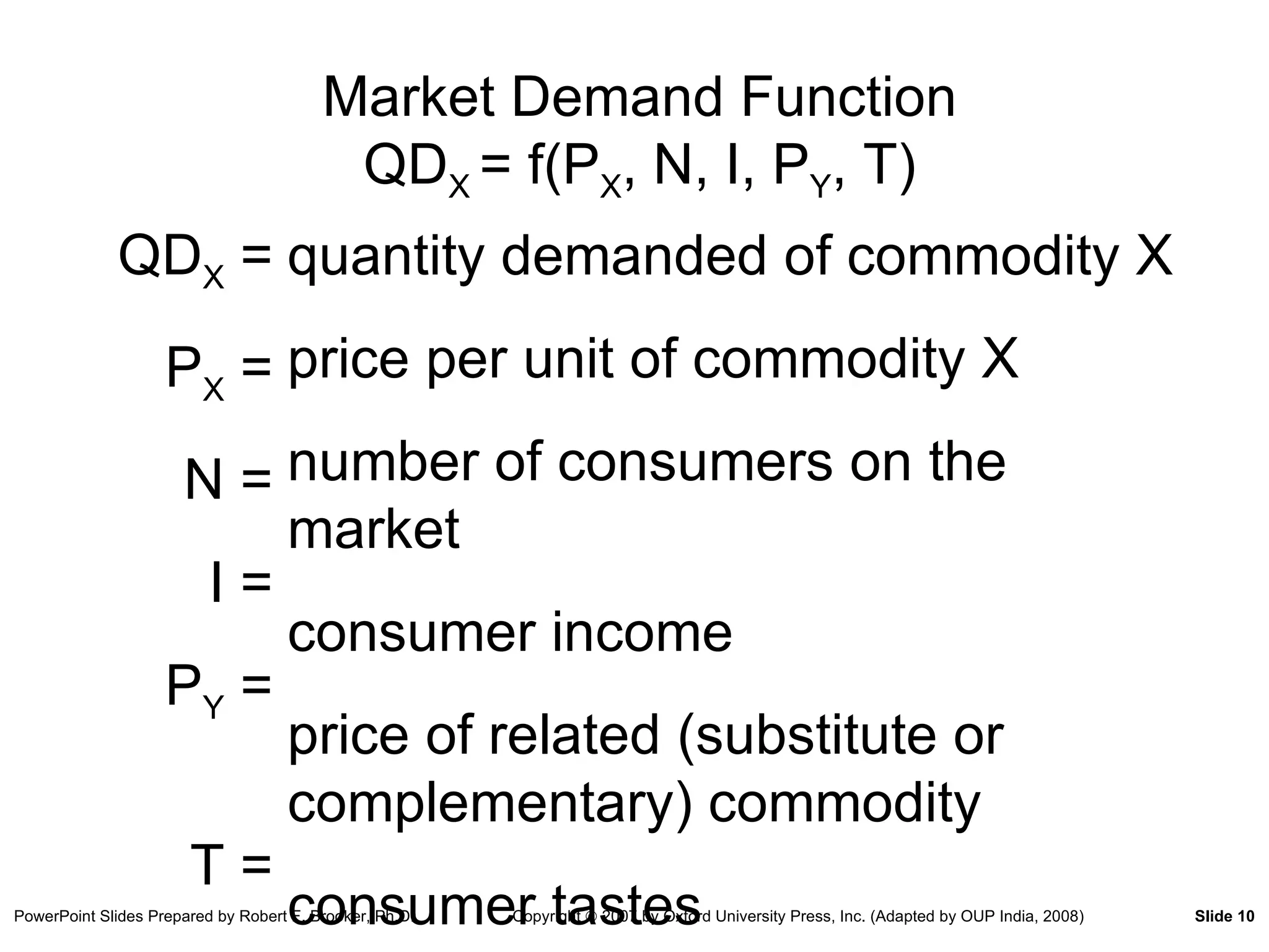
10. Market Demand Function QD X = f(P X , N, I, P Y , T) quantity demanded of commodity X price per unit of commodity X number of consumers on the market consumer income price of related (substitute or complementary) commodity consumer tastes QD X = P X = N = I = P Y = T =

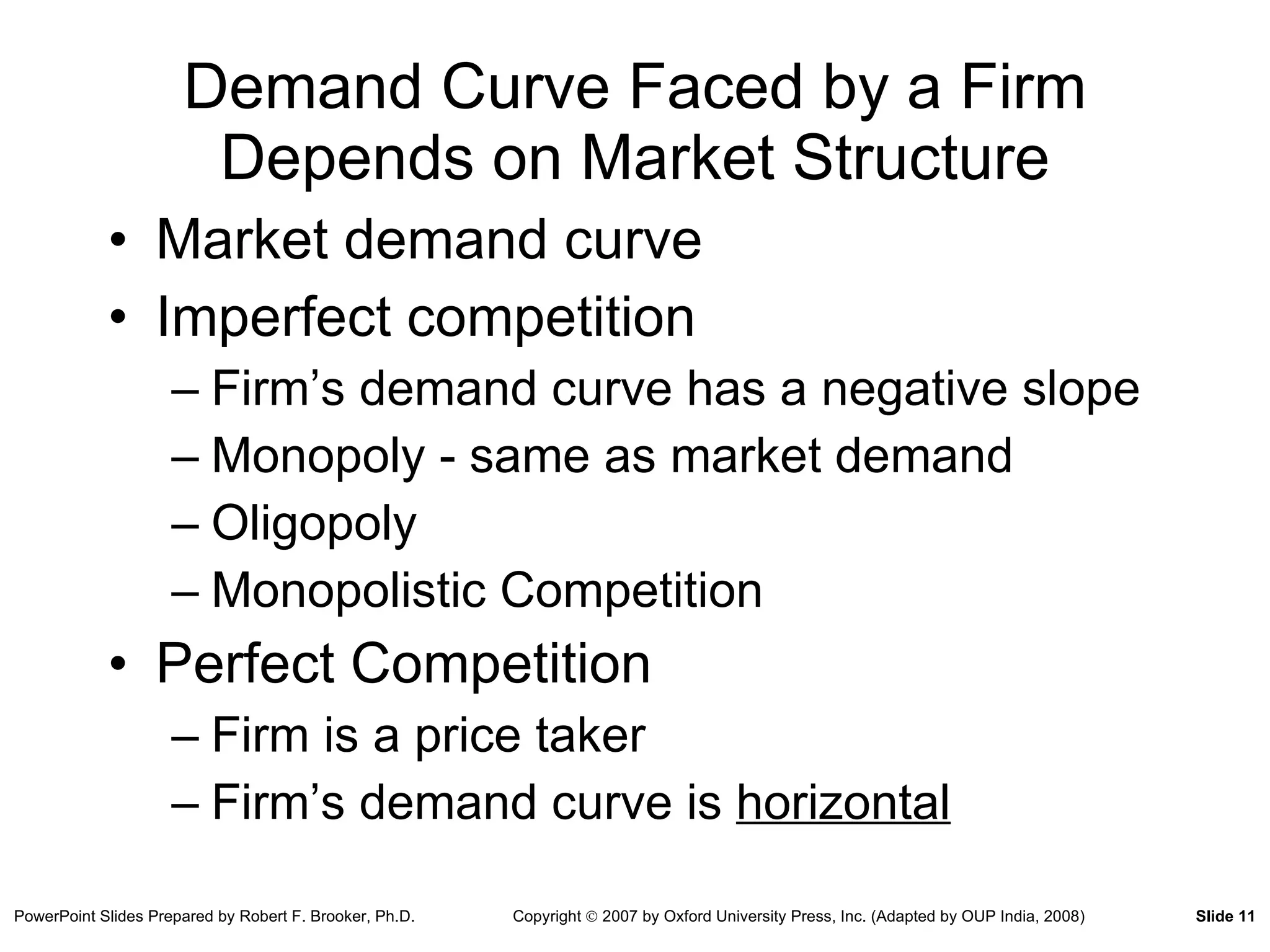
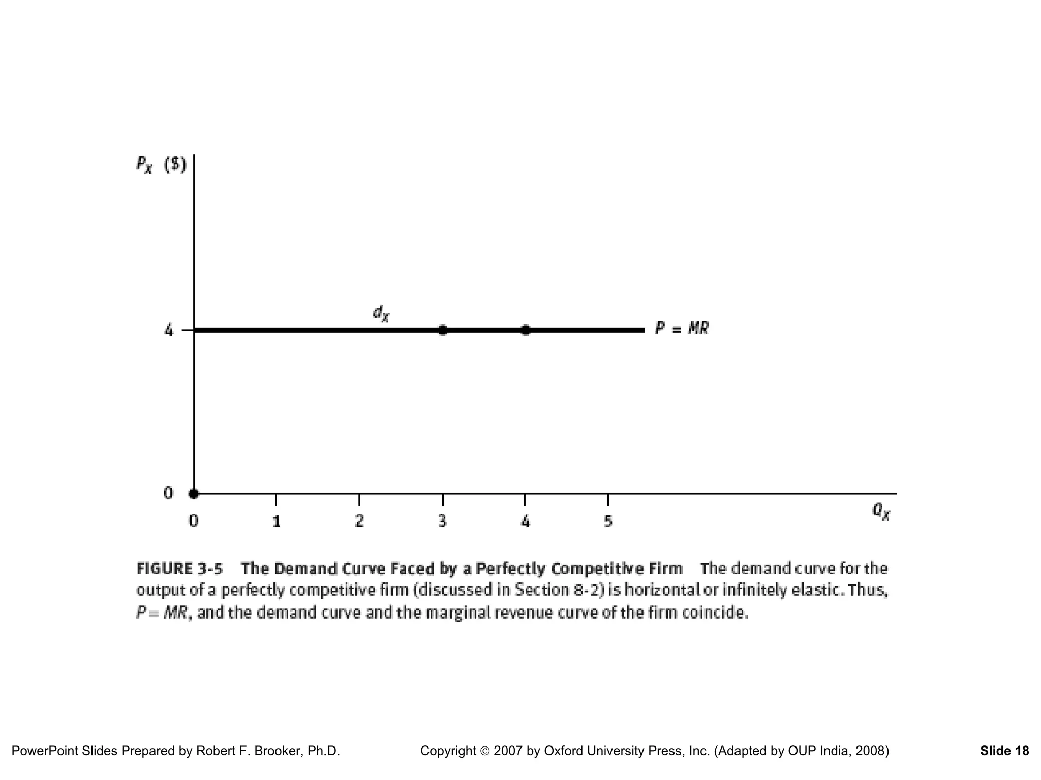
11. Demand Curve Faced by a Firm Depends on Market Structure Market demand curve Imperfect competition Firm’s demand curve has a negative slope Monopoly - same as market demand Oligopoly Monopolistic Competition Perfect Competition Firm is a price taker Firm’s demand curve is horizontal

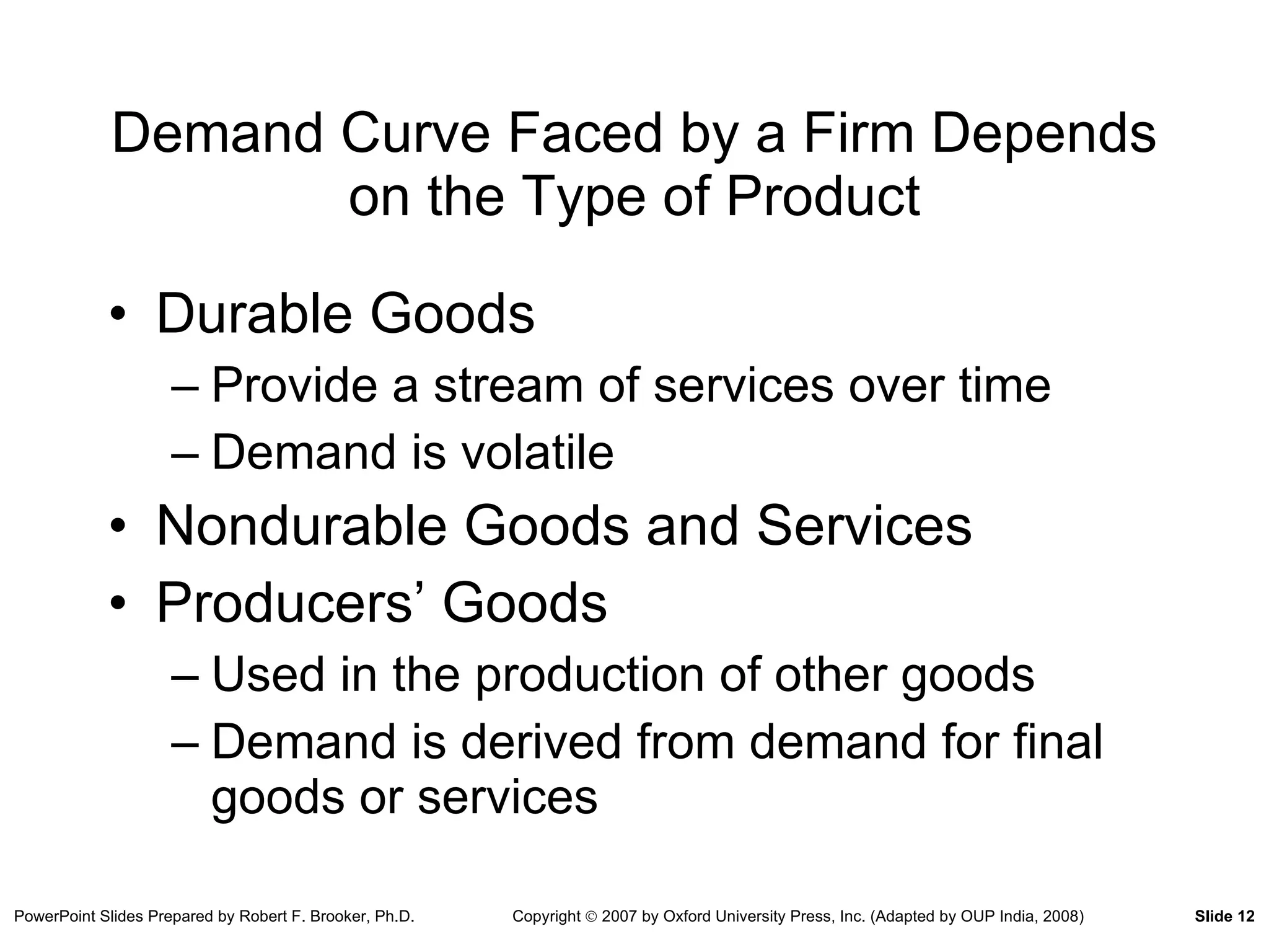
12. Demand Curve Faced by a Firm Depends on the Type of Product Durable Goods Provide a stream of services over time Demand is volatile Nondurable Goods and Services Producers’ Goods Used in the production of other goods Demand is derived from demand for final goods or services

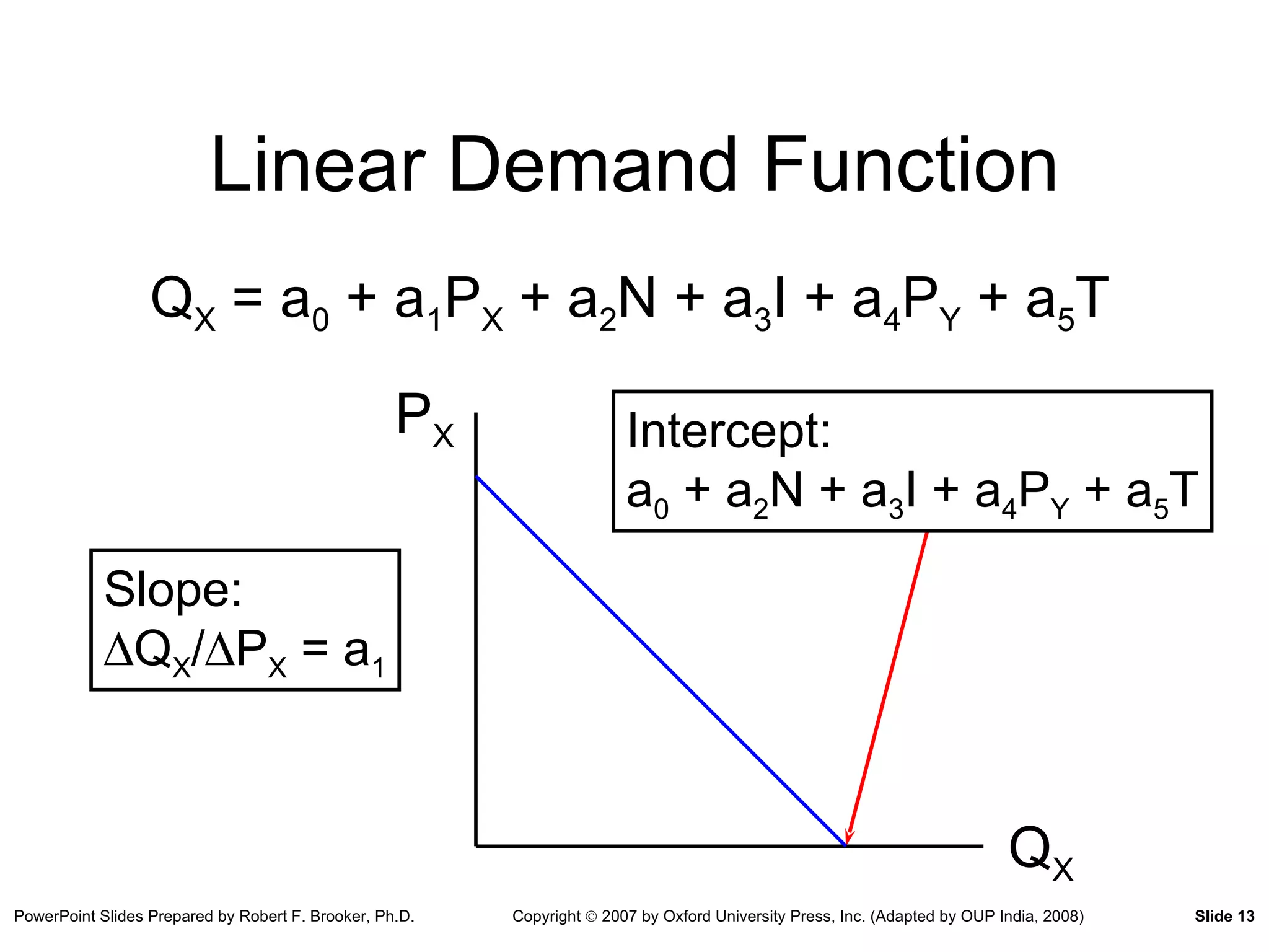
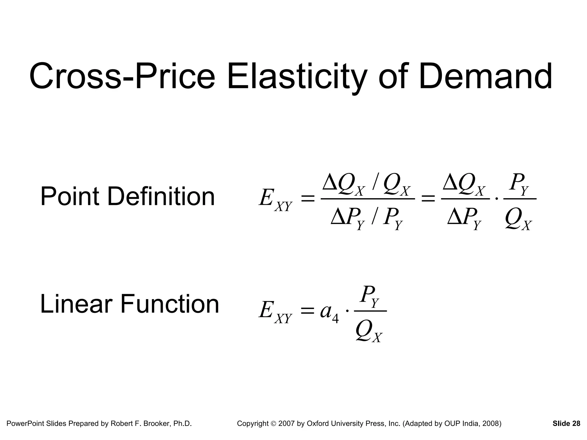
13. Linear Demand Function Q X = a 0 + a 1 P X + a 2 N + a 3 I + a 4 P Y + a 5 T P X Q X Intercept: a 0 + a 2 N + a 3 I + a 4 P Y + a 5 T Slope:  Q X /  P X = a 1

14. Linear Demand Function Example Part 1 Demand Function for Good X Q X = 160 - 10P X + 2N + 0.5I + 2P Y + T Demand Curve for Good X Given N = 58, I = 36, P Y = 12, T = 112 Q = 430 - 10P

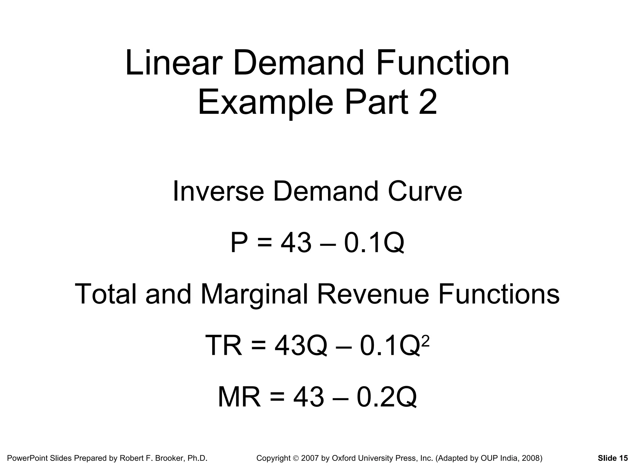
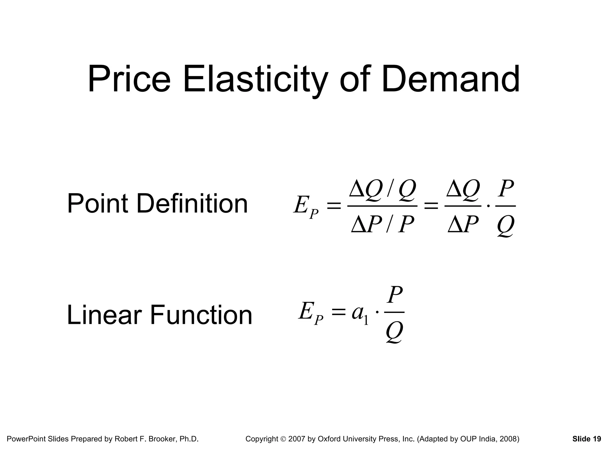
15. Linear Demand Function Example Part 2 Inverse Demand Curve P = 43 – 0.1Q Total and Marginal Revenue Functions TR = 43Q – 0.1Q 2 MR = 43 – 0.2Q

19. Price Elasticity of Demand Linear Function Point Definition

20. Price Elasticity of Demand Arc Definition

21. Marginal Revenue and Price Elasticity of Demand

22. Marginal Revenue and Price Elasticity of Demand P X Q X MR X

23. Marginal Revenue, Total Revenue, and Price Elasticity TR Q X MR<0 MR>0 MR=0

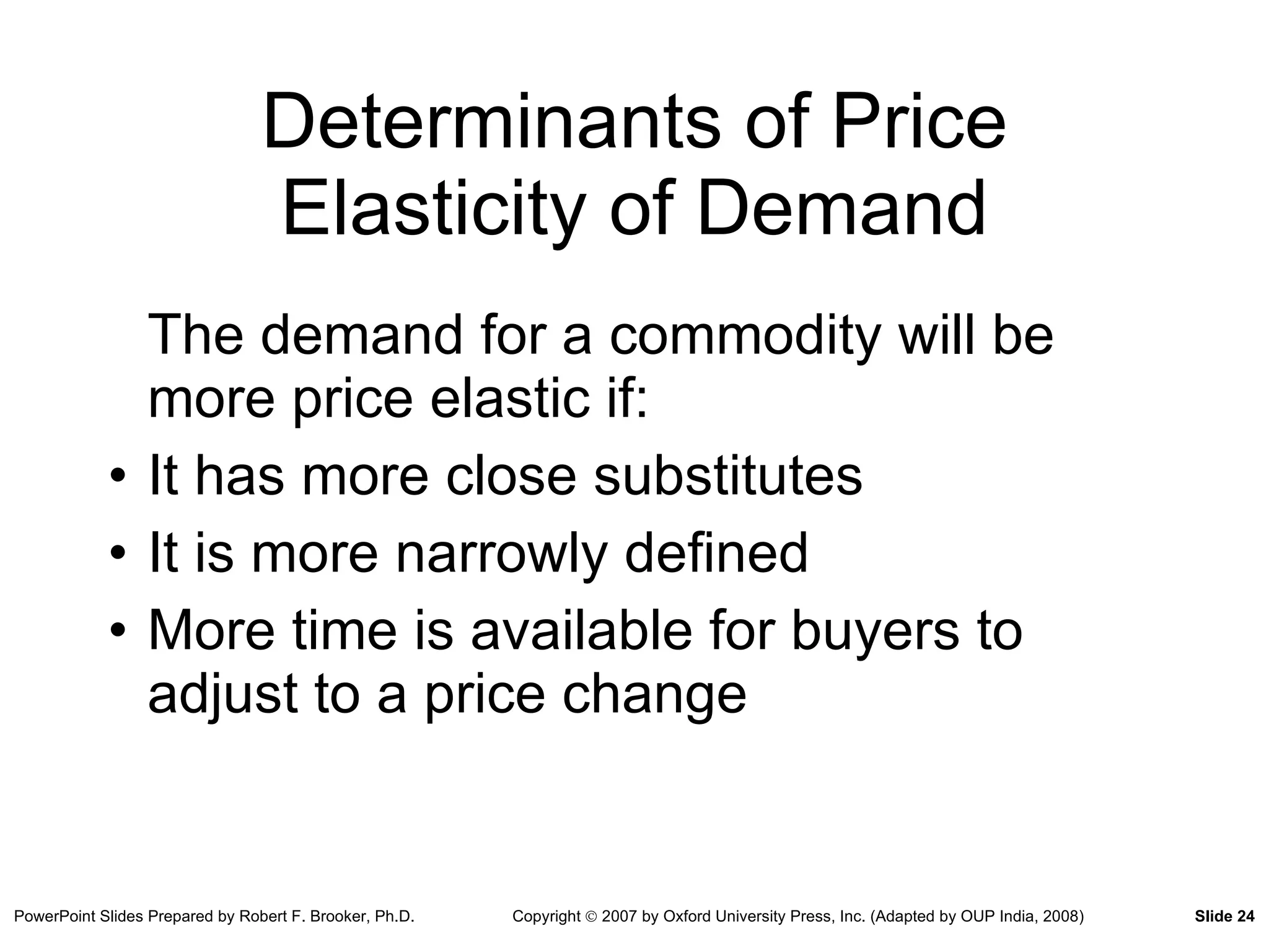
24. Determinants of Price Elasticity of Demand The demand for a commodity will be more price elastic if: It has more close substitutes It is more narrowly defined More time is available for buyers to adjust to a price change

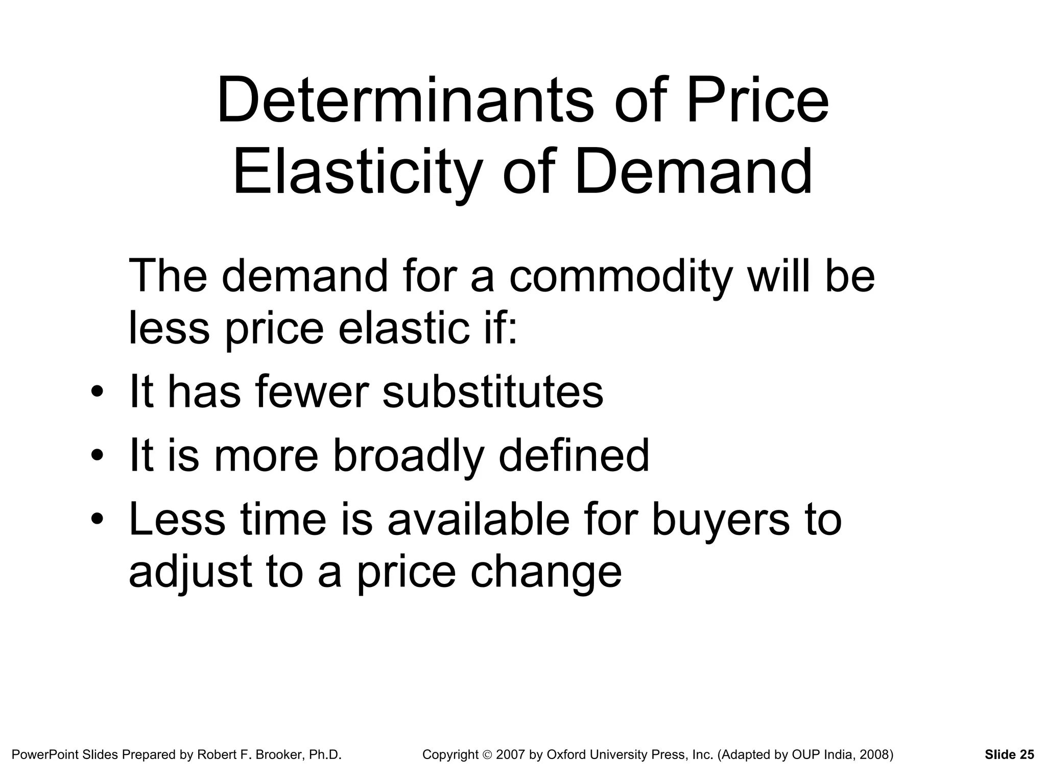
25. Determinants of Price Elasticity of Demand The demand for a commodity will be less price elastic if: It has fewer substitutes It is more broadly defined Less time is available for buyers to adjust to a price change

26. Income Elasticity of Demand Linear Function Point Definition

27. Income Elasticity of Demand Arc Definition Normal Good Inferior Good

28. Cross-Price Elasticity of Demand Linear Function Point Definition

29. Cross-Price Elasticity of Demand Arc Definition Substitutes Complements

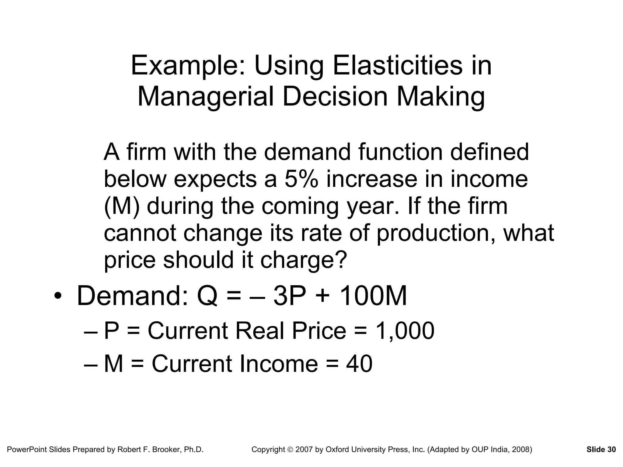
30. Example: Using Elasticities in Managerial Decision Making A firm with the demand function defined below expects a 5% increase in income (M) during the coming year. If the firm cannot change its rate of production, what price should it charge? Demand: Q = – 3P + 100M P = Current Real Price = 1,000 M = Current Income = 40

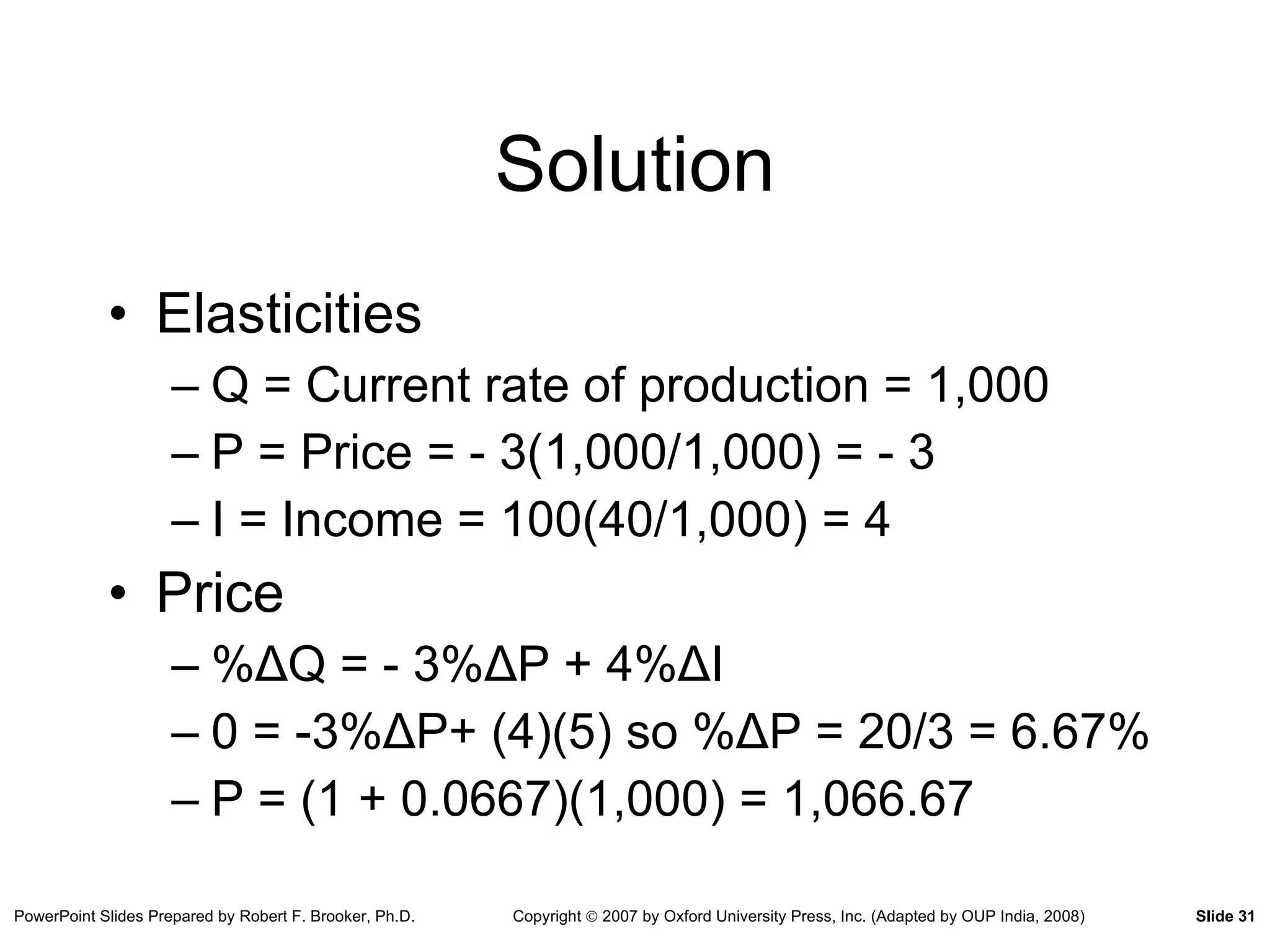
31. Solution Elasticities Q = Current rate of production = 1,000 P = Price = - 3(1,000/1,000) = - 3 I = Income = 100(40/1,000) = 4 Price % Δ Q = - 3 % Δ P + 4 % Δ I 0 = -3 % Δ P+ (4)(5) so % Δ P = 20/3 = 6.67% P = (1 + 0.0667)(1,000) = 1,066.67

32. Other Factors Related to Demand Theory International Convergence of Tastes Globalization of Markets Influence of International Preferences on Market Demand Growth of Electronic Commerce Cost of Sales Supply Chains and Logistics Customer Relationship Management

33. Chapter 3 Appendix

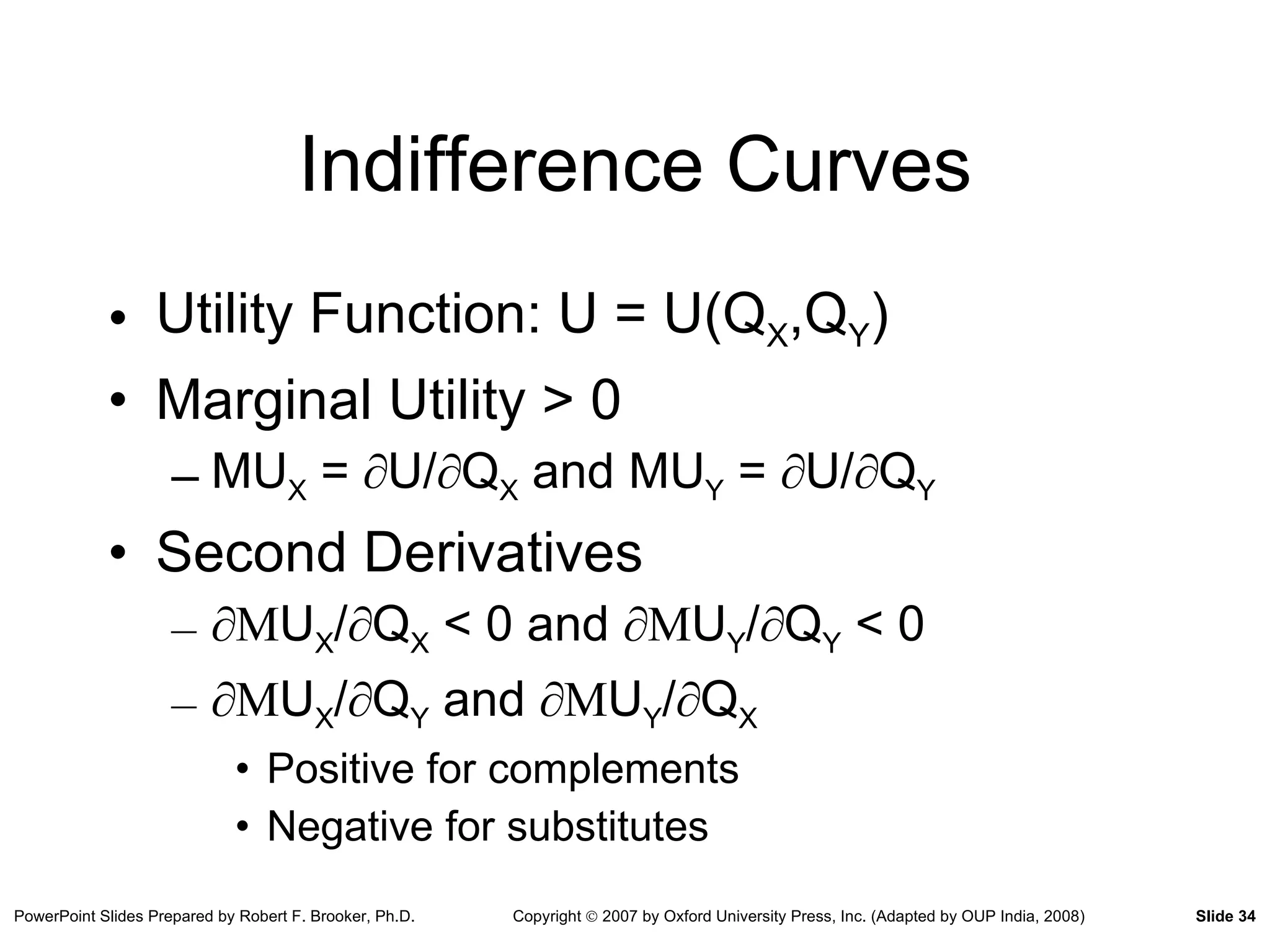
34. Indifference Curves Utility Function: U = U(Q X ,Q Y ) Marginal Utility > 0 MU X = ∂ U/ ∂ Q X and MU Y = ∂ U/ ∂ Q Y Second Derivatives ∂ M U X / ∂ Q X < 0 and ∂M U Y / ∂ Q Y < 0 ∂ M U X / ∂ Q Y and ∂M U Y / ∂ Q X Positive for complements Negative for substitutes

35. Marginal Rate of Substitution Rate at which one good can be substituted for another while holding utility constant Slope of an indifference curve dQ Y /dQ X = -MU X /MU Y

37. Indifference Curves: Complements and Substitutes Perfect Complements Perfect Substitutes Q Y Q X Q Y Q X

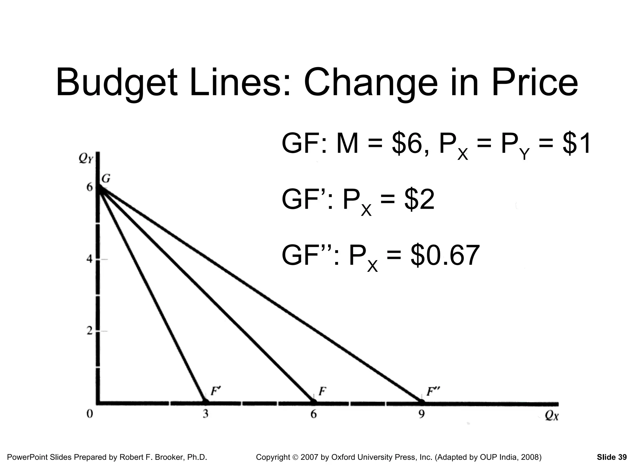
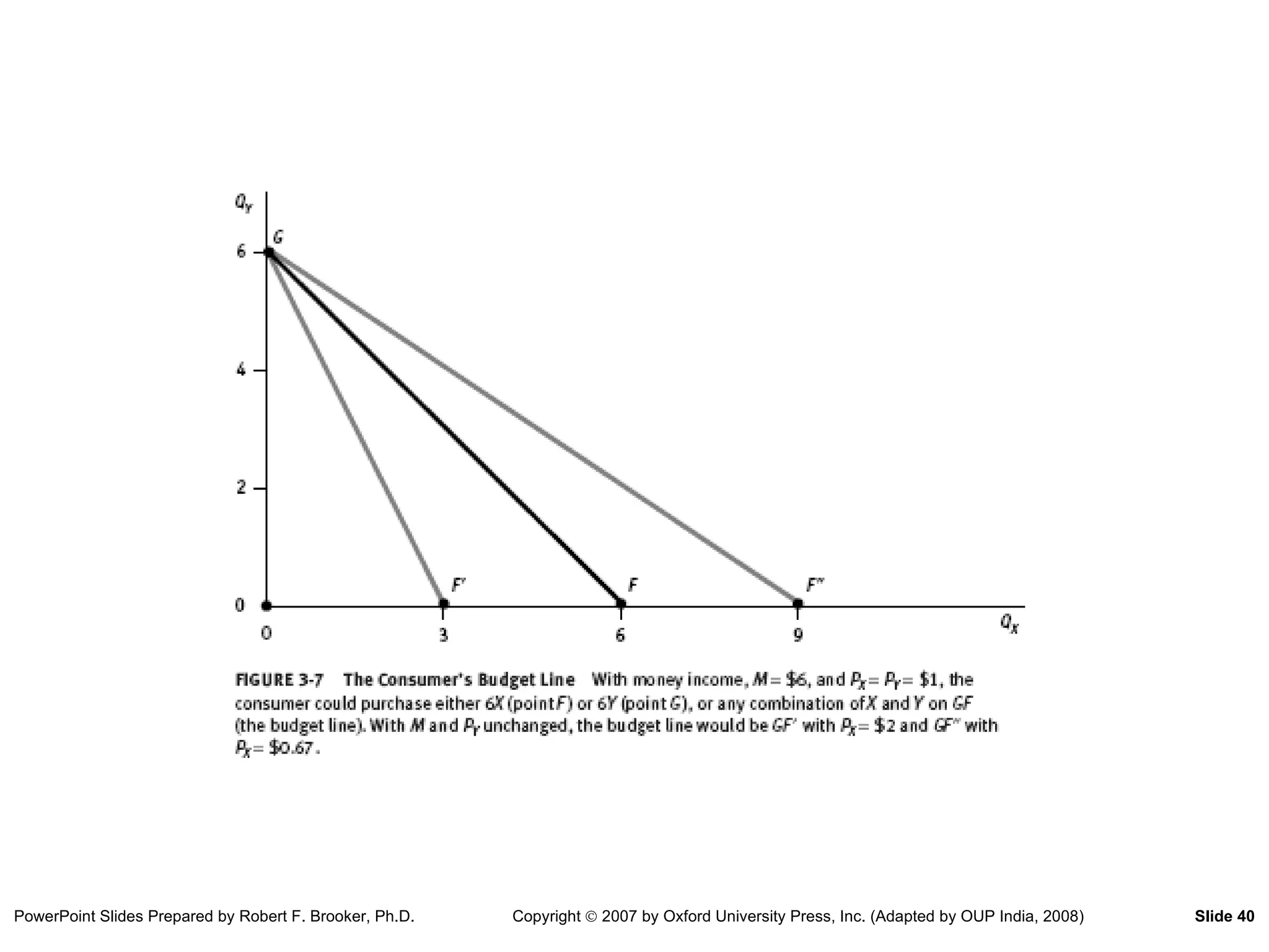
38. The Budget Line Budget = M = P X Q X + P Y Q Y Slope of the budget line Q Y = M/P Y - (P X /P Y )Q X dQ Y /dQ X = - P X /P Y

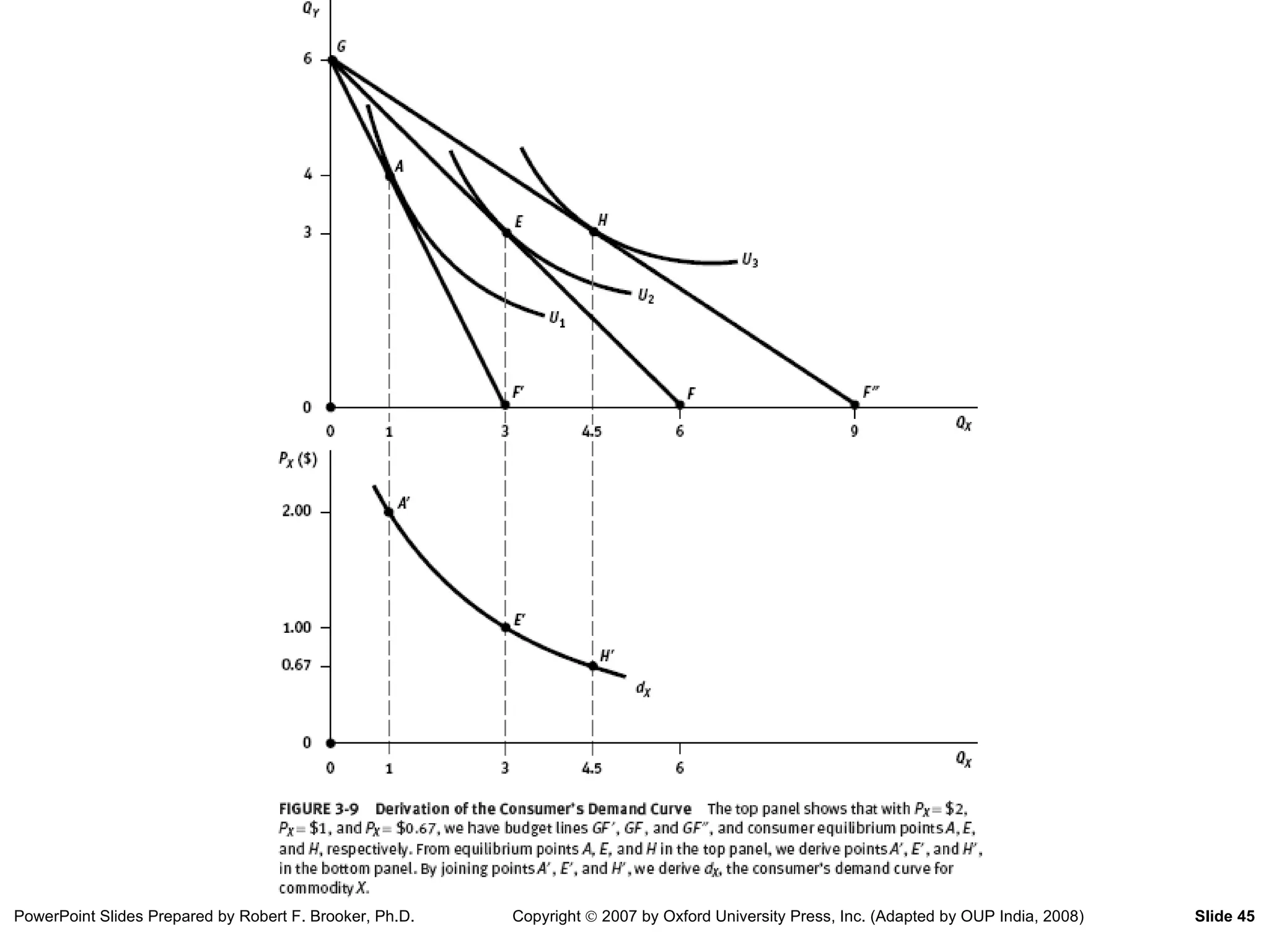
39. Budget Lines: Change in Price GF: M = $6, P X = P Y = $1 GF’: P X = $2 GF’’: P X = $0.67

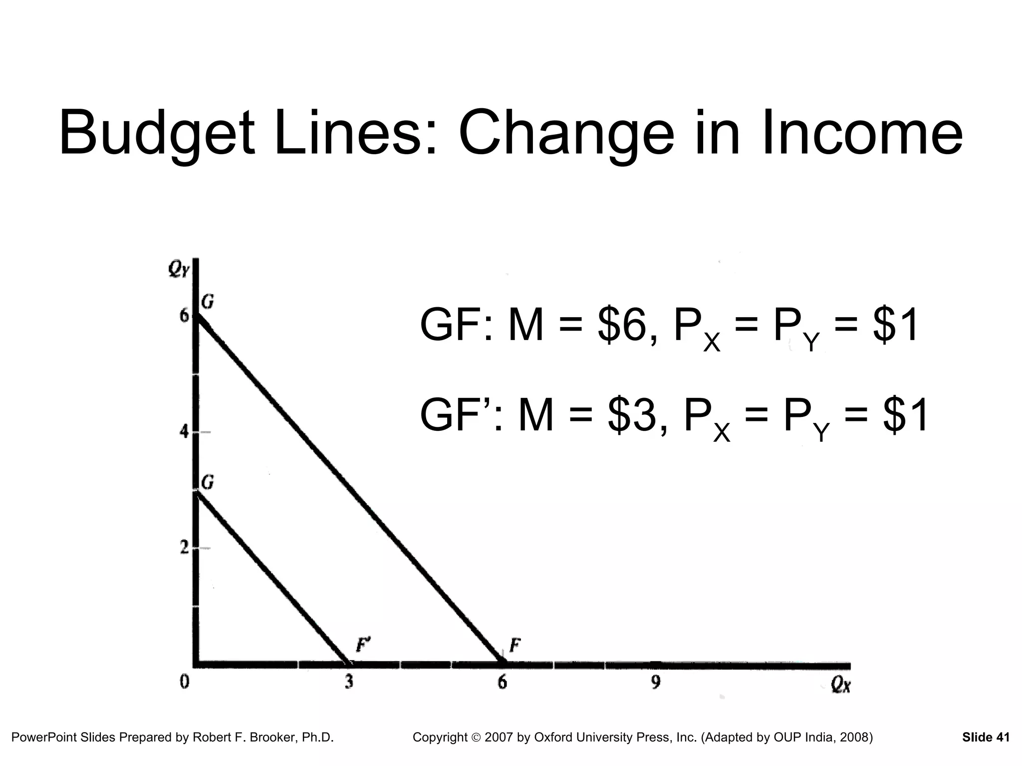
41. Budget Lines: Change in Income GF: M = $6, P X = P Y = $1 GF’: M = $3, P X = P Y = $1

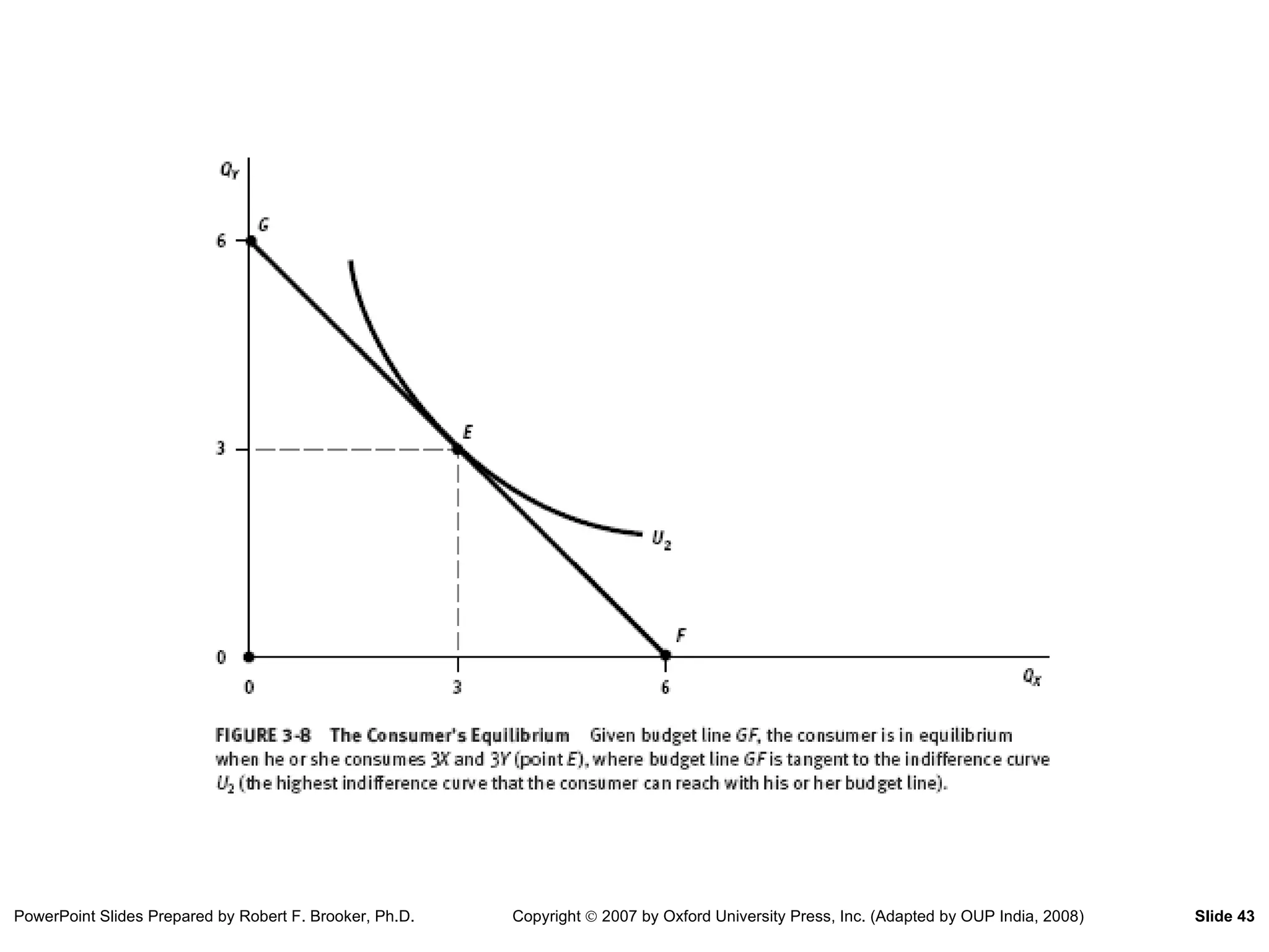
42. Consumer Equilibrium Combination of goods that maximizes utility for a given set of prices and a given level of income Represented graphically by the point of tangency between an indifference curve and the budget line MU X /MU Y = P X /P Y MU X /P X = MU Y /P Y

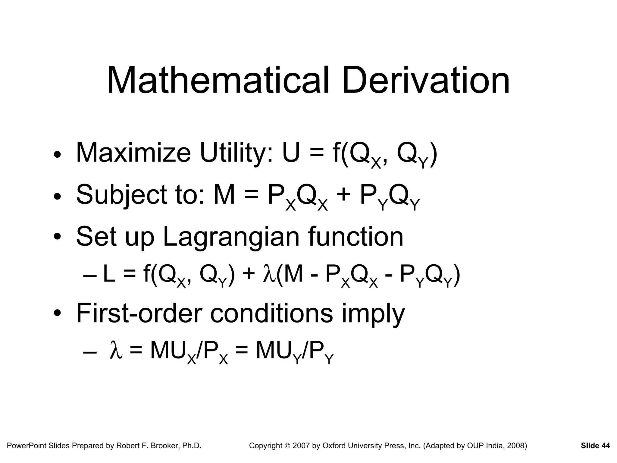
44. Mathematical Derivation Maximize Utility: U = f(Q X , Q Y ) Subject to: M = P X Q X + P Y Q Y Set up Lagrangian function L = f(Q X , Q Y ) +  (M - P X Q X - P Y Q Y ) First-order conditions imply  = MU X /P X = MU Y /P Y