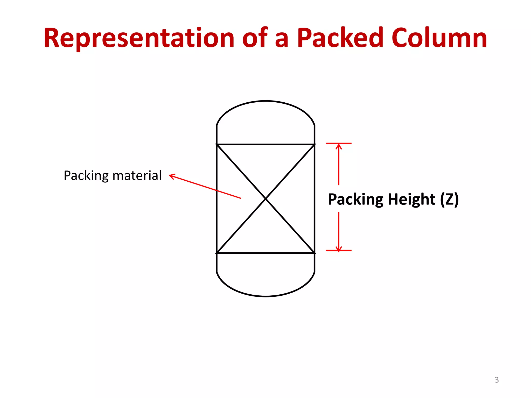
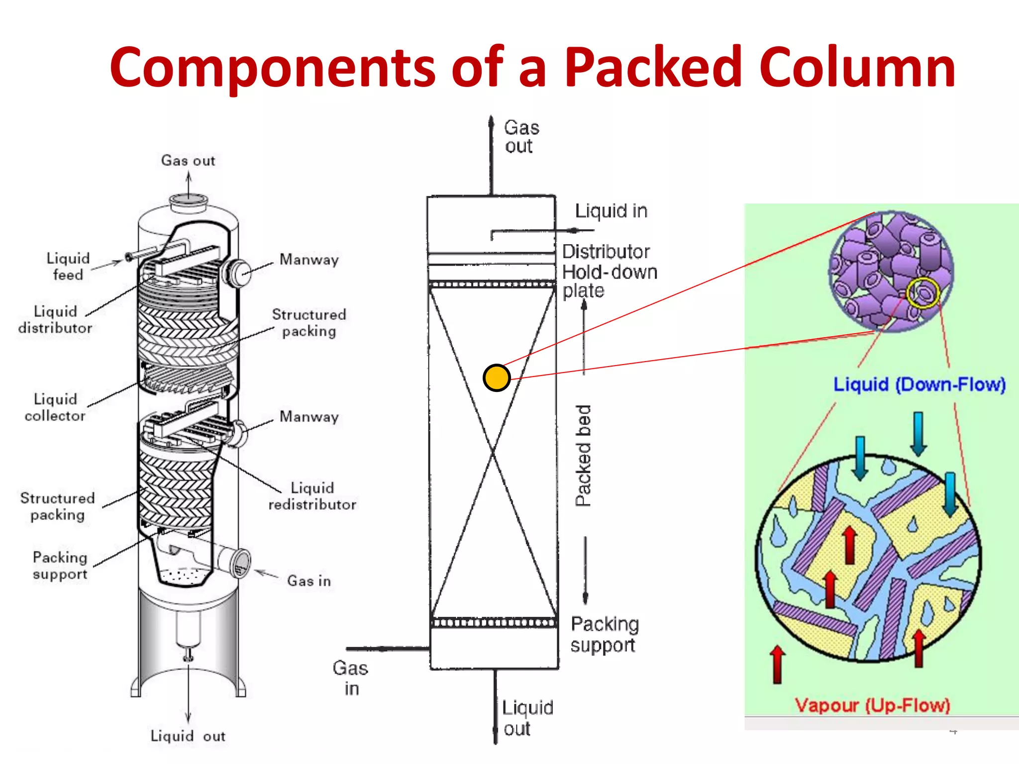
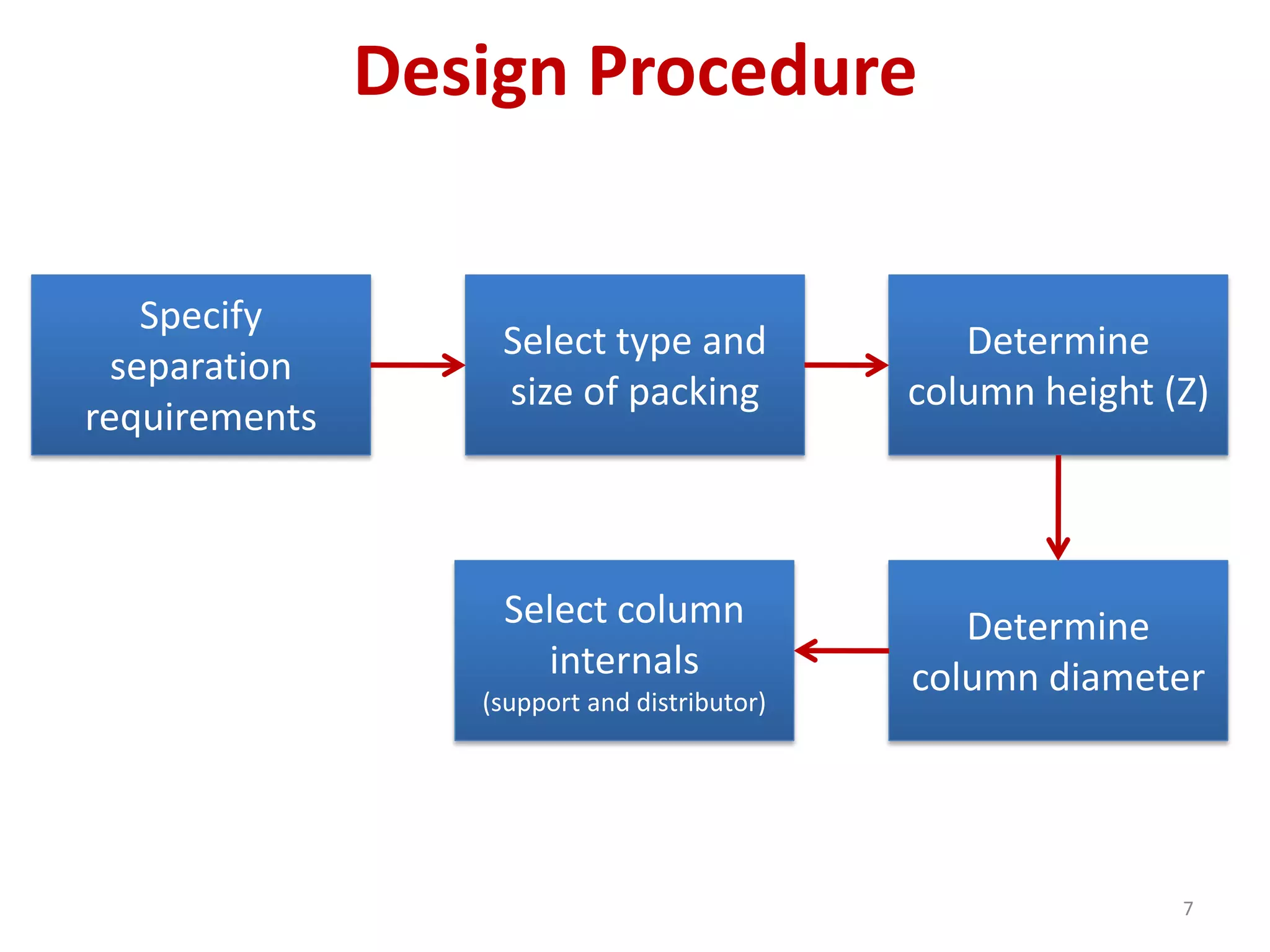
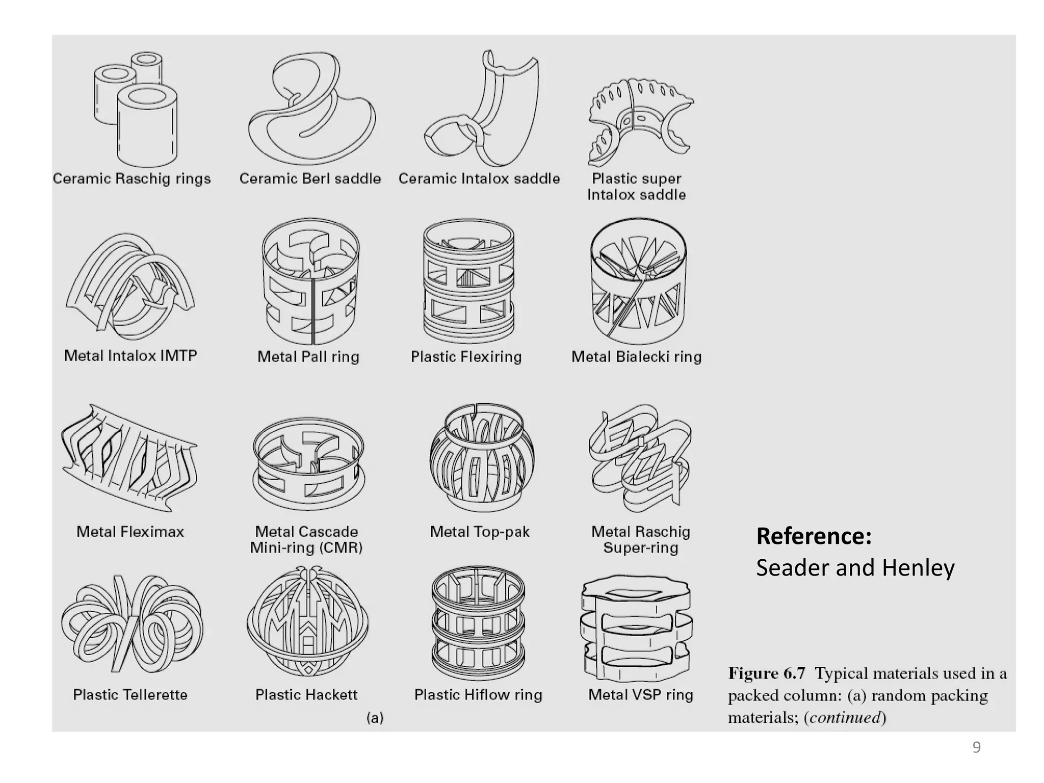
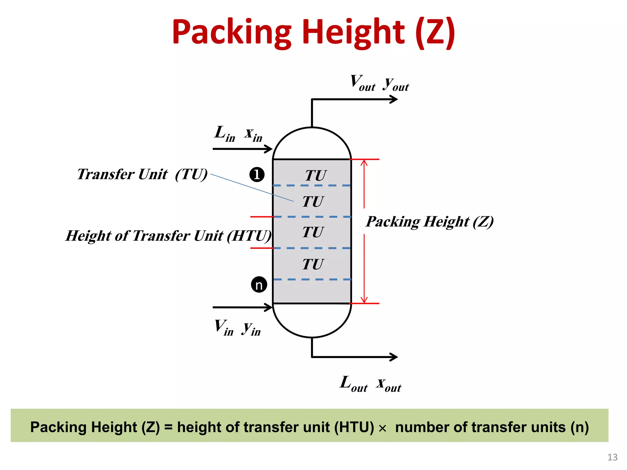
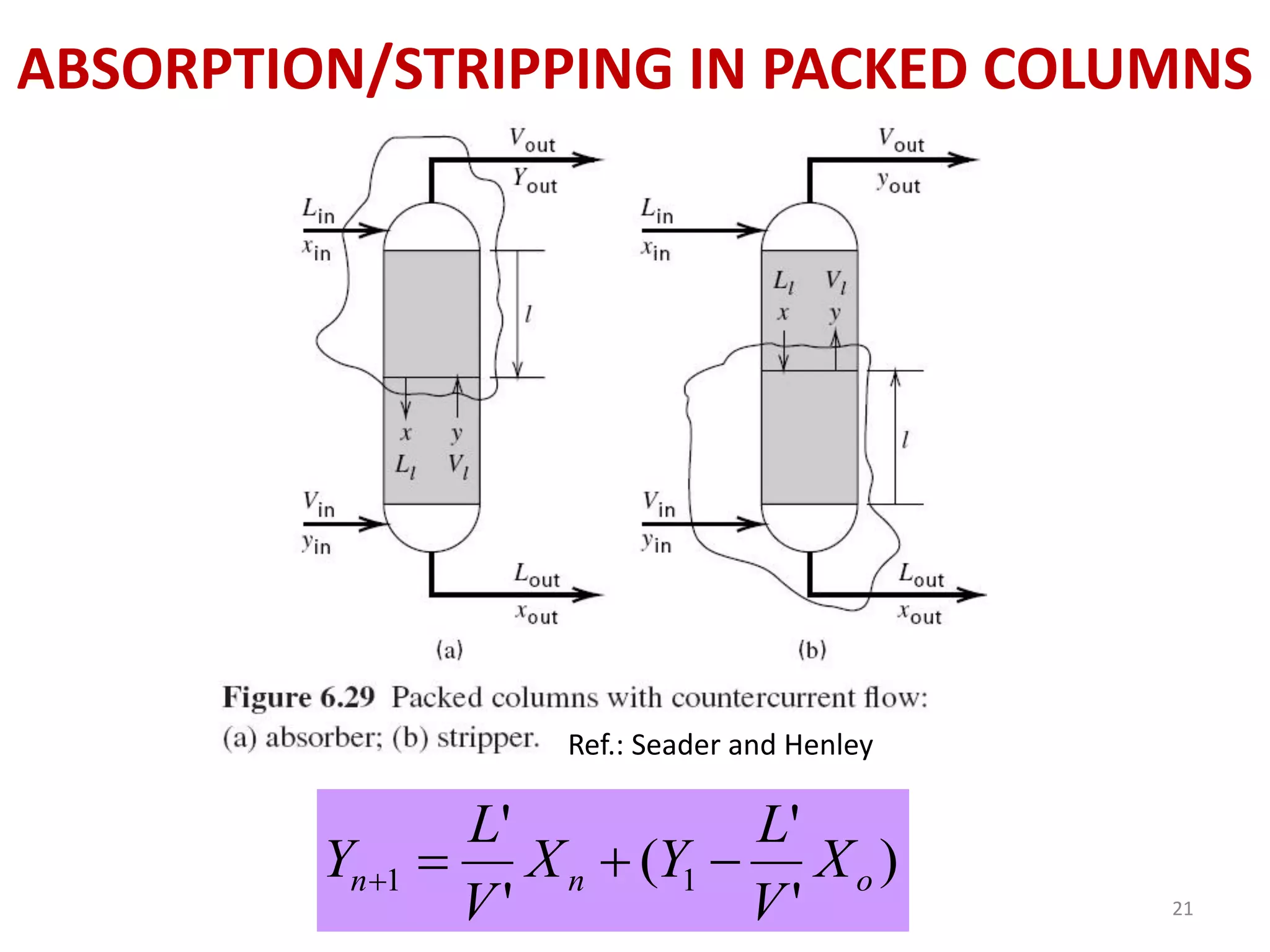
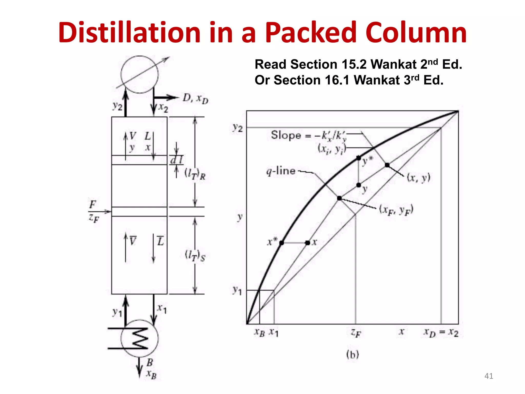
Packed columns are used for distillation, gas absorption, and liquid-liquid extraction. They have continuous gas-liquid contact through a packed bed, unlike plate columns which have stage-wise contact. Packed columns depend on good liquid and gas distribution, and have lower holdup but higher pressure drop than plate columns. This document provides details on packed column components, design procedures such as selecting packing and determining height, and examples of absorption and stripping processes in packed columns.

1. 1
References
1. Wankat: 10.6  10.9 and 15.1  15.6
2. Coulson & Richardson (Vol 6): 11.14
3. Seader and Henley (Vol 2): Chapter 6
Dr. Hatem Alsyouri
Heat and Mass Transfer Operations
Chemical Engineering Department
The University of Jordan

2. Packed Columns
• Packed columns are used for distillation, gas absorption,
and liquid-liquid extraction.
• The gas liquid contact in a packed bed column is
continuous, not stage-wise, as in a plate column.
• The liquid flows down the column over the packing surface
and the gas or vapor, counter-currently, up the column.
Some gas-absorption columns are co-current
• The performance of a packed column is very dependent on
the maintenance of good liquid and gas distribution
throughout the packed bed.
2

3. 3
Representation of a Packed Column
Packing material
Packing Height (Z)

4. Components of a Packed Column
4

5. Advantages of Trayed Columns
1) Plate columns can handle a wider range of liquid and gas flow-rates
than packed columns.
2) Packed columns are not suitable for very low liquid rates.
3) The efficiency of a plate can be predicted with more certainty than the
equivalent term for packing (HETP or HTU).
4) Plate columns can be designed with more assurance than packed
columns. There is always some doubt that good liquid distribution can
be maintained throughout a packed column under all operating
conditions, particularly in large columns.
5) It is easier to make cooling in a plate column; coils can be installed on
the plates.
6) It is easier to have withdrawal of side-streams from plate columns.
7) If the liquid causes fouling, or contains solids, it is easier to provide
cleaning in a plate column; manways can be installed on the plates. With
small diameter columns it may be cheaper to use packing and replace
the packing when it becomes fouled.
5

6. Advantages of Packed Columns
1. For corrosive liquids, a packed column will usually be cheaper
than the equivalent plate column.
2. The liquid hold-up is lower in a packed column than a plate
column. This can be important when the inventory of toxic or
flammable liquids needs to be kept as small as possible for
safety reasons.
3. Packed columns are more suitable for handling foaming
systems.
4. The pressure drop can be lower for packing than plates; and
packing should be considered for vacuum columns.
5. Packing should always be considered for small diameter
columns, say less than 0.6 m, where plates would be difficult
to install, and expensive.
6

7. 7
Design Procedure
Select type and
size of packing
Determine
column height (Z)
Determine
column diameter
Specify
separation
requirements
Select column
internals
(support and distributor)

8. Packing Materials
1. Ceramic: superior wettability, corrosion
resistance at elevated temperature, bad
strength
2. Metal: superior strength & good wettability
3. Plastic: inexpensive, good strength but may
have poor wettability at low liquid rate
8

9. Reference:
Seader and Henley
9

10. Structured
packing materials
Reference:
Seader and Henley10

11. 11
Characteristics of Packing
Reference:
Seader and Henley

12. 12
Reference:
Seader and Henley

13. Packing Height (Z)
n

Lin xin
Vin yin
Vout yout
Lout xout
TU
TU
TU
TU
Height of Transfer Unit (HTU)
Transfer Unit (TU)
Packing Height (Z)
Packing Height (Z) = height of transfer unit (HTU)  number of transfer units (n)
13

14. Methods for Packing Height (Z)
14
2 methods
Equilibrium stage
analysis
HETP method
Mass Transfer
analysis
HTU method
Z = HETP  N
N = number of theoretical stages obtained from
McCabe-Thiele method
HETP
• Height Equivalent to a Theoretical Plate
• Represents the height of packing that gives
similar separation to as a theoretical stage.
• HETP values are provided for each type of
packing
Z = HTU  NTU
HTU = Height of a Transfer unit
NTU = Number of Transfer Units (obtained by
numerical integration)
More common
 

outA
inA
y
y AAcy yy
dy
AaK
V
Z
)( *
 

outA
inA
x
x AA
A
cx xx
xd
AaK
L
Z
)( *
OGOG NHZ 
OLOL NHZ 

15. 15
Evaluating height based on HTU-NTU model
 

outA
inA
y
y AAcy yy
dy
AaK
V
Z
)( *
HOG
Integration = NOG
• NOG is evaluated graphically by numerical integration using the equilibrium and
operating lines.
• Draw 1/(yA
* -yA) (on y-axis) vs. yA (on x-axis). Area under the curve is the value
of integration.
Substitute values to calculate HOG
y
x
)(
1
*
AA yy  Evaluate area
under the curve
by numerical
integration
Area = N

16. 16
Two-Film Theory of Mass Transfer
(Ref.: Seader and Henley)
Overall
gas phase or Liquid phase
Gas phase Boundary layer Liq phase Boundary layer
Local
gas phase
Local
liq phaseAt a specific
location in
the column

17. Phase LOCAL coefficient OVERALL coefficient
Gas Phase Z = HG  NG
M. Transfer Coeff.: ky a
Driving force: (y – yi)
Z = HOG  NOG
M. Transfer Coeff.: Ky a
Driving force: (y – y*)
Liquid
Phase
Z = HL  NL
M. Transfer Coeff.: kx a
Driving force: (x – xi)
Z = HOL  NOL
M. Transfer Coeff.: Kx a
Driving force: (x – x*)
17
Alternative Mass Transfer Grouping
Note: Driving force could be ( y – yi) or (yi – y) is decided based on direction of flow. This
applies to gas and liquid phases, overall and local.

18. 18
yA yA
*
(yA
*
-yA) 1/(yA
*
-yA)
yA in   
   
yA out   
A
y
y AA
y
y AA
A
OG dy
yyyy
dy
N
outA
inA
outA
inA
 



)(
1
)( **
• Use Equilibrium data related to process (e.g., x-y for absorption
and stripping) and the operating line (from mass balance).
• Obtain data of the integral in the given range and fill in the table
• Draw yA vs. 1/(yA *- yA)
• Then find area under the curve graphically or numerically
Graphical evaluation of N (integral)
Assume we are evaluating
yin
yout

19. 19
Distillation random case
Equilibrium line
operating lines

20. 20
7 point Simpson’s rule:
 )()(4)(2)(4)(2)(4)(
3
)( 6543210
6
0
XfXfXfXfXfXfXf
h
dXXf
X
X

 
6
06 XX
h


Simpson’s Rule for approximating the integral
 )()(4)(2)(4)(
3
)( 43210
4
0
XfXfXfXfXf
h
dXXf
X
X

 
4
04 XX
h


5 points Simpson’s rule:
 )()(4)(
3
)( 210
2
0
XfXfXf
h
dXXf
X
X
  
2
02 XX
h


3 points Simpson’s rule:

21. ABSORPTION/STRIPPING IN PACKED COLUMNS
)
'
'
(
'
'
11 onn X
V
L
YX
V
L
Y 
21
Ref.: Seader and Henley

22. 22

23. 23

24. Counter-current Absorption (local gas phase)
24
X
Y
Y1
Y out
Yout
Y in
Xin
Xin
X out
X out
Y in
Y2
Y3
Y4
Y5
Y3 i
ak
ak
slope
y
x


25. Counter-current Absorption (overall gas phase)
25
X
Y
Y1
Y out
Yout
Y in
Xin
Xin
X out
X out
Y in
Y2
Y3
Y4
Y5
Y3
*
vertical

26. Counter-current Absorption (local liquid phase)
26
X
Y
Y out
Yout
Y in
Xin
X1
X out
X 4
Y in
X3 i
ak
ak
slope
y
x

Xin
X out
X2
X 3

27. Counter-current Absorption (overall liquid phase)
27
X
Y
Y out
Yout
Y in
Xin
X1
X out
X 4
Y in
X3
*
Xin
X out
X2
X 3
horizontal

28. 28
Note: This exercise (from Seader and Henley) was solved using an equation
based on a certain approximation. You need to re-solve it graphically using
Simspon’s rule and compare the results.

29. 29

30. 30

31. Stripping Exercise
Wankat 15D8
31
We wish to strip SO2 from water using air at 20C.
The inlet air is pure. The outlet water contains
0.0001 mole fraction SO2, while the inlet water
contains 0.0011 mole fraction SO2. Operation is
at 855 mmHg and L/V = 0.9×(L/V)max. Assume
HOL = 2.76 feet and that the Henry’s law
constant is 22,500 mmHg/mole frac SO2.
Calculate the packing height required.

32. 32
 Ptot = 855 mmHg
 H = 22,500 mmHg SO2 /mole frac SO2
 pSO2 = H xSO2
 ySO2 Ptot = H xSO2
 ySO2 = (H/ Ptot) x SO2
or ySO2 = m x SO2
where m = (H/ Ptot) = 22,500/855
= 26.3 (used to draw equilibrium
data)
Draw over the range of interest,
i.e., from x=0 to x= 11104
at x= 0  y = 0
at x= 11104  y = 26.3 * 11104
= 0.02893 = 28.93 104
Air (solvent)
V
yin = 0
Solution
xout = 0.0001
= 1104
Water
L
xin = 0.0011
= 11104
T = 20C
P = 855 mmHg

33. 33
0
5
10
15
20
25
30
35
40
0 2 4 6 8 10 12 14 16
ySO2103
x SO2 104
xin
11104
xout
1104

34. 34
 V(yout – yout) = L( xin-xout)  V(yout – 0) = L( 11x10-4-1x10-4)
yout= 10x10-4 (L/V)
(L/V) = 0.9 (L/V)max
From pinch point and darwing, (L/V)max = slope= 29.29
(L/V) = 0.9  29.29 = 26.36
yout= 10x10-4 (L/V) = 10x10-4  26.36
 yout = 0.02636 = 26.36103
Draw actual operating line

35. 35
0
5
10
15
20
25
30
35
40
0 2 4 6 8 10 12 14 16
ySO2103
x SO2 104
xin
11104
xout
1104

36. 36
0
5
10
15
20
25
30
0 2 4 6 8 10 12
ySO2103
x SO2  104

37. 37
0
5
10
15
20
25
30
0 2 4 6 8 10 12
ySO2103
x SO2 104

38. 38
x x* 1/(x-x*)
1.0E-4 0 10,000
3.0E-04 2.0E-04 10,000
5.0E-04 4.0E-04 10,000
7.0E-04 6.0E-04 10,000
9.0E-04 8.0E-04 10,000
1.1E-03 1.0E-03 10,000
Apply a graphical
or numerical
method for
evaluating NOL
For example, we can use Simpson’s rule. The 7 point
Simpson’s rule defined as follows:




0011.0
0001.0
)( *
inA
outA
x
x AA xx
dx
  )()(4)(2)(4)(2)(4)(
36
)( 6543210
06
6
0
XfXfXfXfXfXfXf
XX
dXXf
X
X




 )()(4)(2)(4)(2)(4)(
3
)( 6543210
6
0
XfXfXfXfXfXfXf
h
dXXf
X
X

 
6
06 XX
h



39. 39
Substituting values from Table gives NOL= 9.5.
Z = HOL(given)  NOL(calculated) = 2.76  9.5
 Z = 26.22 ft
  )()(4)(2)(4)(2)(4)(
36
)( 6543210
06
6
0
XfXfXfXfXfXfXf
XX
dXXf
X
X








0011.0
0001.0
)( *
inA
outA
x
x AA xx
dx
)(
1
)( *
xx
Xf



40. 40
5-point method
 )()(4)(2)(4)(
3
)( 43210
4
0
XfXfXfXfXf
h
dXXf
X
X

 
4
04 XX
h


Pay attention to accuracy
of drawing and obtaining
data.
Grades will be subtracted
in case of hand drawing!

41. Distillation in a Packed Column
41
Read Section 15.2 Wankat 2nd Ed.
Or Section 16.1 Wankat 3rd Ed.

42. 42
1. Feed
2. Distillate
3. Bottom
4. Reflux
5. Boilup
6. Rectifying section
7. Striping section
8. Condenser
9. Re-boiler
10. Tray (plate or stage)
11. Number of Trays
12. Feed tray

43. 43
𝑉 𝐿
𝐿𝑉 Rectifying
Stripping

44. Graphical
Design
Method
Binary
mixtures
Equilibrium and Operating Lines
44

45. 45
NTUHTU
𝑁 𝐺 =
𝑦 𝑖𝑛
𝑦 𝑜𝑢𝑡
𝑑𝑦 𝐴
𝑦 𝐴𝑖 − 𝑦 𝐴
𝐻 𝐺 =
𝑉
𝑘 𝑦 𝑎 𝐴 𝑐
𝑁𝐿 =
𝑥 𝑜𝑢𝑡
𝑥 𝑖𝑛
𝑑𝑥 𝐴
𝑥 𝐴 − 𝑥 𝐴𝑖
𝐻𝐿 =
𝐿
𝑘 𝑥 𝑎 𝐴 𝑐
𝑁 𝑂𝐺 =
𝑦 𝑖𝑛
𝑦 𝑜𝑢𝑡
𝑑𝑦 𝐴
𝑦 𝐴
∗
− 𝑦 𝐴
𝐻 𝑂𝐺 =
𝑉
𝐾 𝑦 𝑎 𝐴 𝑐
𝑁 𝑂𝐿 =
𝑥 𝑖𝑛
𝑥 𝑜𝑢𝑡
𝑑𝑥 𝐴
𝑥 𝐴 − 𝑥 𝐴
∗
𝐻 𝑂𝐿 =
𝐿
𝐾𝑥 𝑎 𝐴 𝑐
𝑦 𝐴𝑖−𝑦 𝐴
𝑥 𝐴𝑖−𝑥 𝐴
=
−𝑘 𝑥 𝑎
𝑘 𝑦 𝑎
=
−𝐿
𝑉
𝐻 𝐺
𝐻 𝐿
Slope of tie line
NTUHTU
𝑁 𝐺 =
𝑦 𝑖𝑛
𝑦 𝑜𝑢𝑡
𝑑𝑦 𝐴
𝑦 𝐴𝑖 − 𝑦 𝐴
𝐻 𝐺 =
𝑉
𝑘 𝑦 𝑎 𝐴 𝑐
𝑁𝐿 =
𝑥 𝑜𝑢𝑡
𝑥 𝑖𝑛
𝑑𝑥 𝐴
𝑥 𝐴 − 𝑥 𝐴𝑖
𝐻𝐿 =
𝐿
𝑘 𝑋 𝑎 𝐴 𝑐
𝑁 𝑂𝐺 =
𝑦 𝑖𝑛
𝑦 𝑜𝑢𝑡
𝑑𝑦 𝐴
𝑦 𝐴
∗
− 𝑦 𝐴
𝐻 𝑂𝐺 =
𝑉
𝐾 𝑦 𝑎 𝐴 𝑐
𝑁 𝑂𝐿 =
𝑥 𝑖𝑛
𝑥 𝑜𝑢𝑡
𝑑𝑥 𝐴
𝑥 𝐴 − 𝑥 𝐴
∗
𝐻 𝑂𝐿 =
𝐿
𝐾𝑥 𝑎 𝐴 𝑐
𝑦 𝐴𝑖−𝑦 𝐴
𝑥 𝐴𝑖−𝑥 𝐴
=
−𝑘 𝑥 𝑎
𝑘 𝑦 𝑎
=
− 𝐿
𝑉
𝐻 𝐺
𝐻 𝐿
Slope of tie line
Rectifying section Stripping section

46. 46
L
G
y
x
AAi
AAi
H
H
V
L
ak
ak
xx
yy





yA i
xA i
xA
yA

47. 47
Example 15-1 Wankat (pages 109 and 509)

48. Distillation Exercise 15D4 (Wankat)
48

49. 49

50. 50

51. 51
ya yai (yai-ya) 1/(yai-ya)
0.04 0.13 0.09 11.11
0.3225 0.455 0.1325 7.55
0.605 0.63 0.025 40.00
0.605 0.62 0.015 66.67
0.7625 0.8 0.0375 26.67
0.92 0.95 0.03 33.33

52. • Read sections 10.7 to 10.9 Wankat (2nd or 3rd
Ed.)
52
Diameter calculation of Packed Columns