Downloaded 551 times


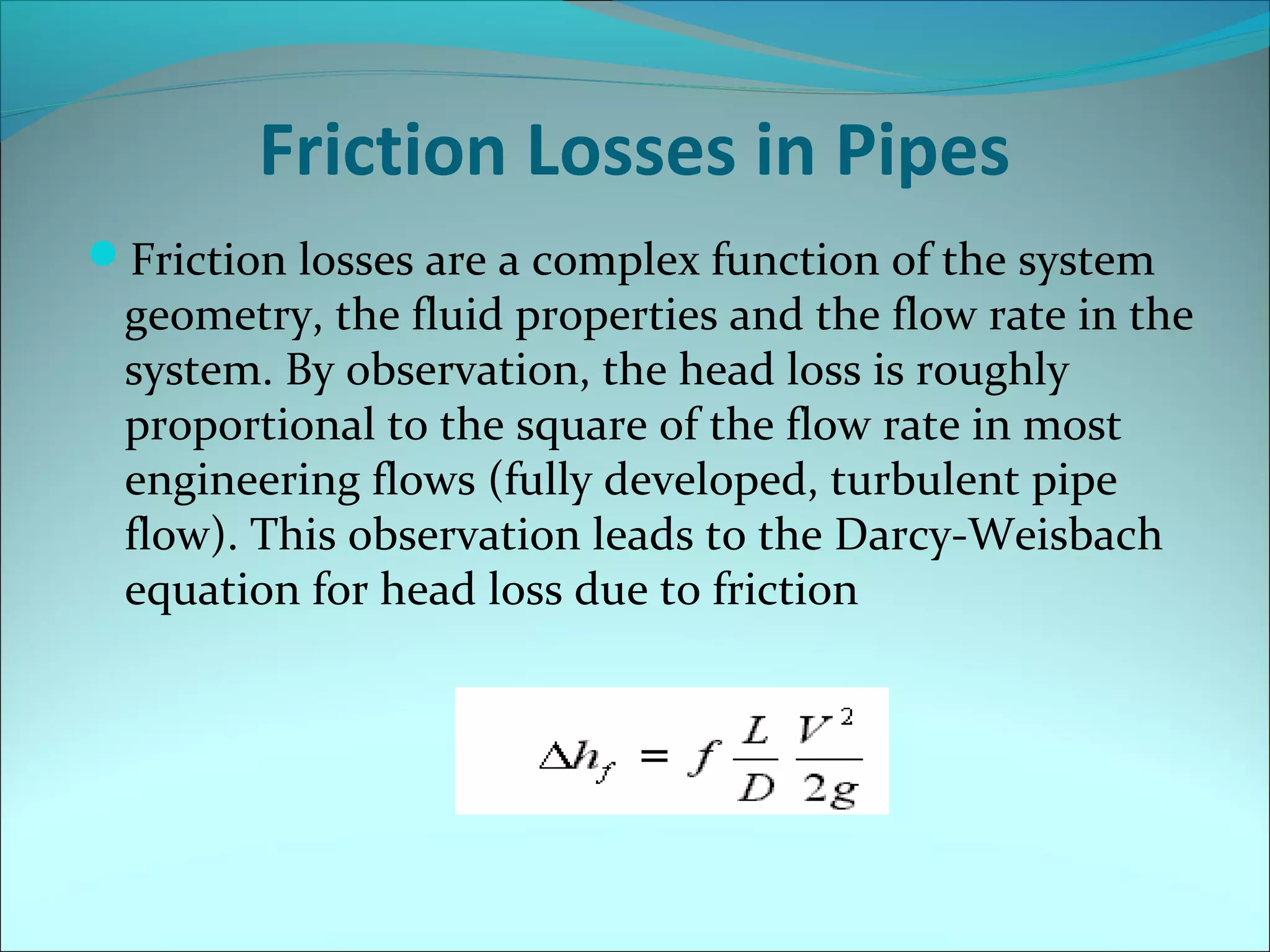
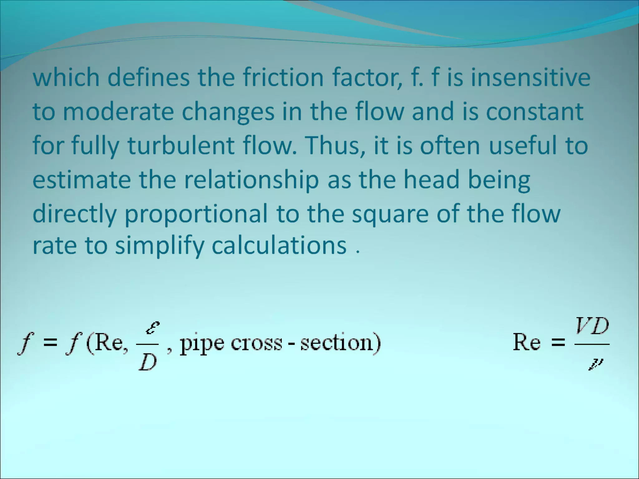

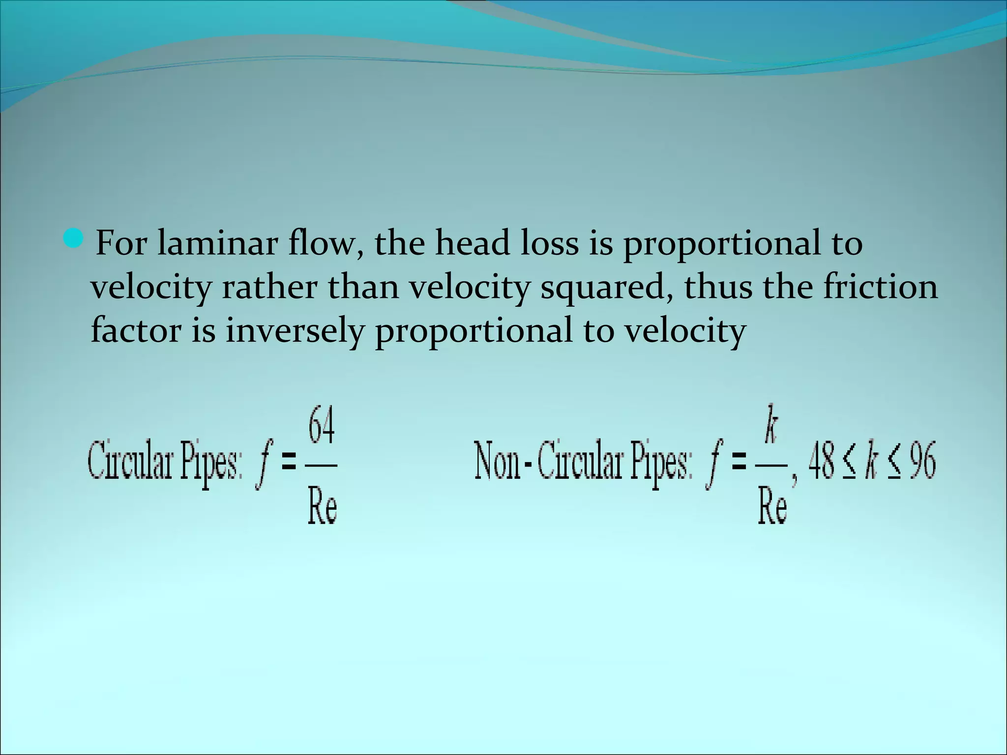


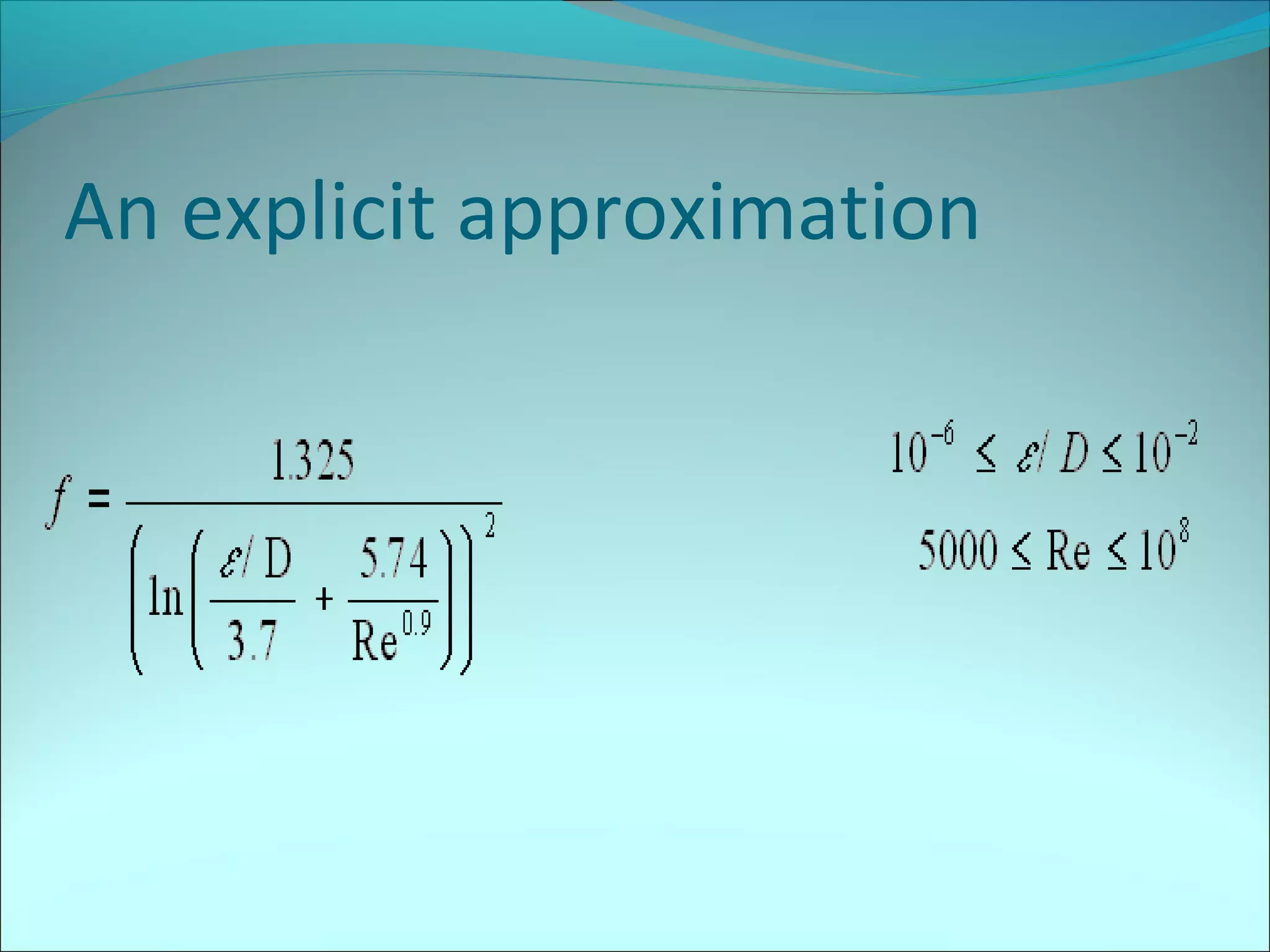


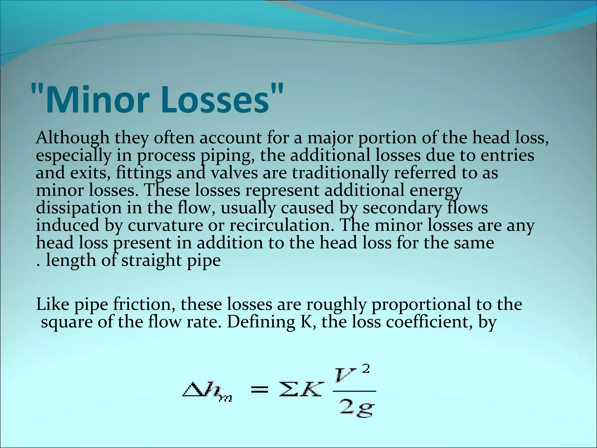
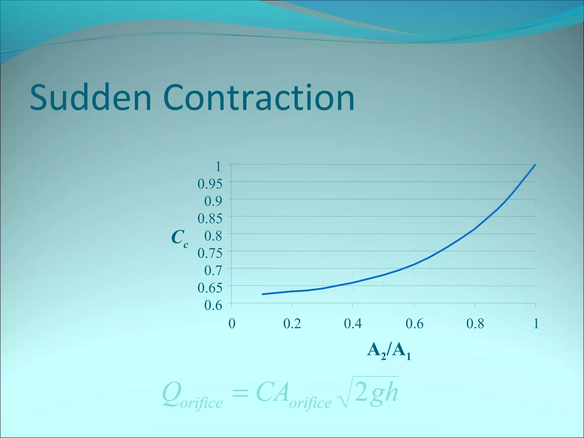
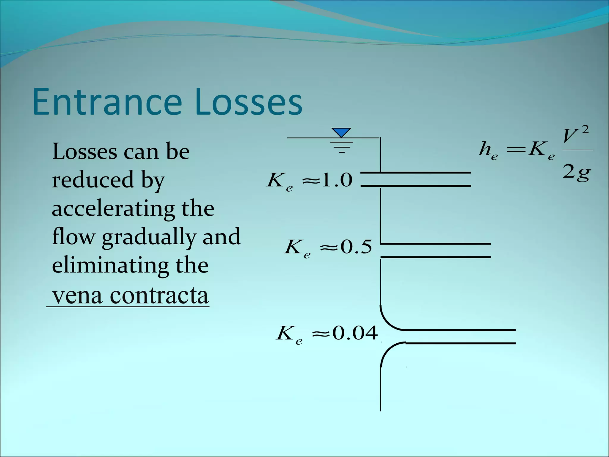

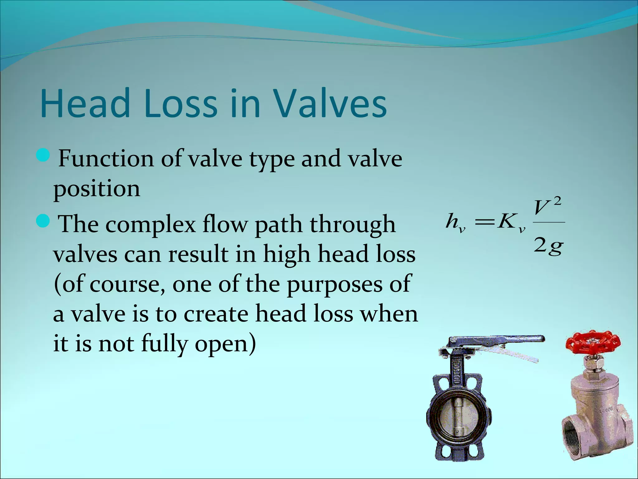
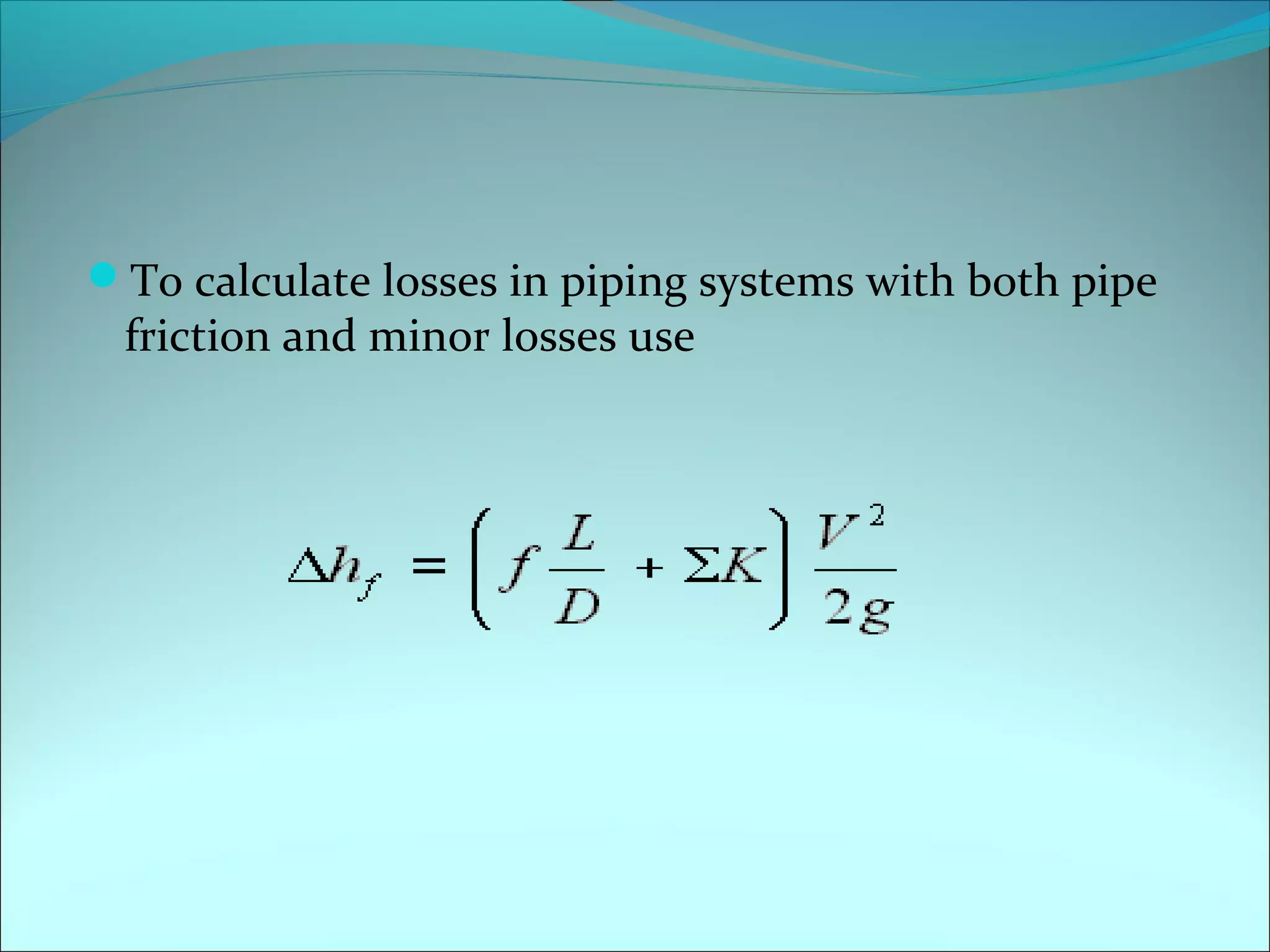


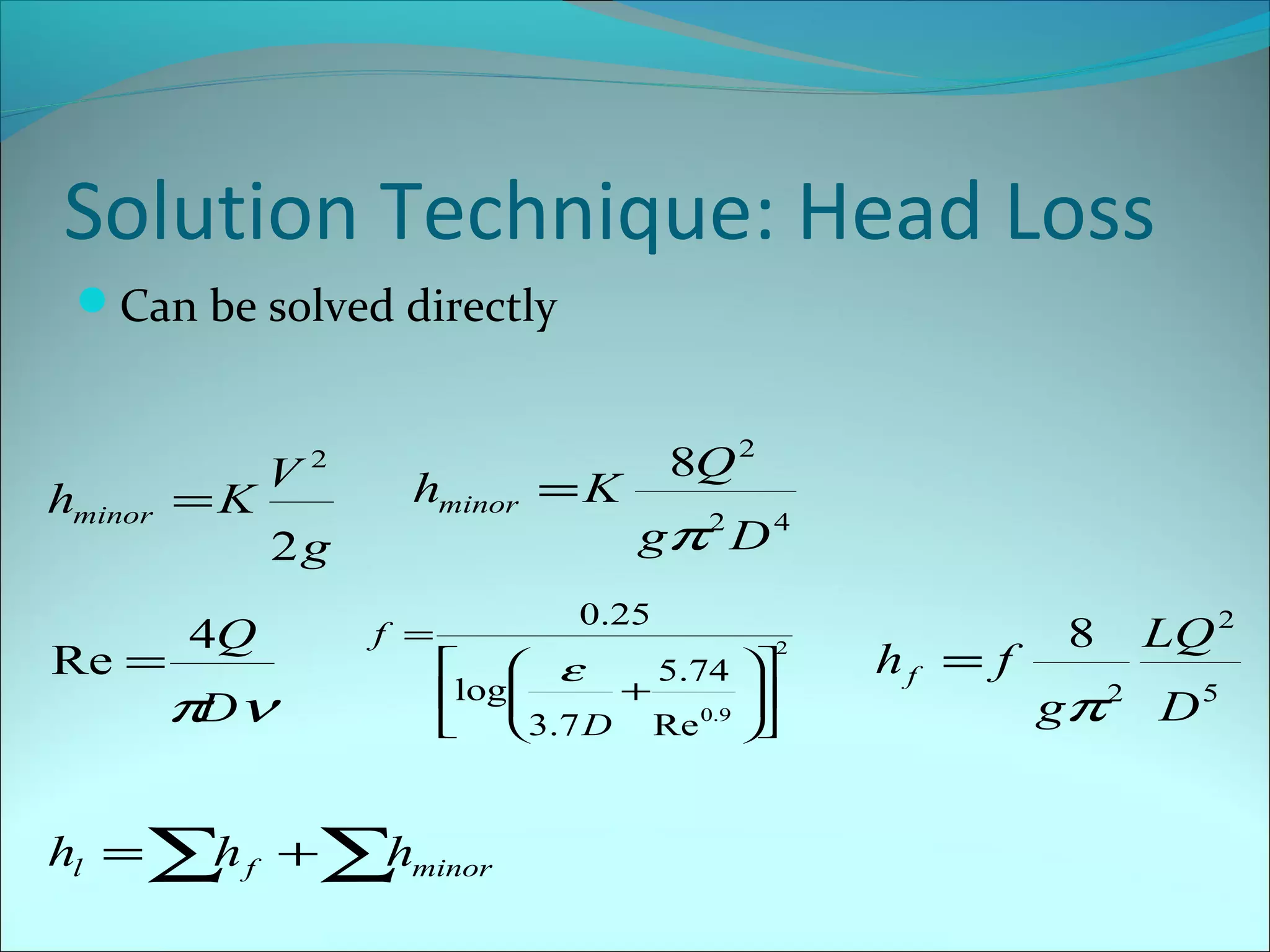

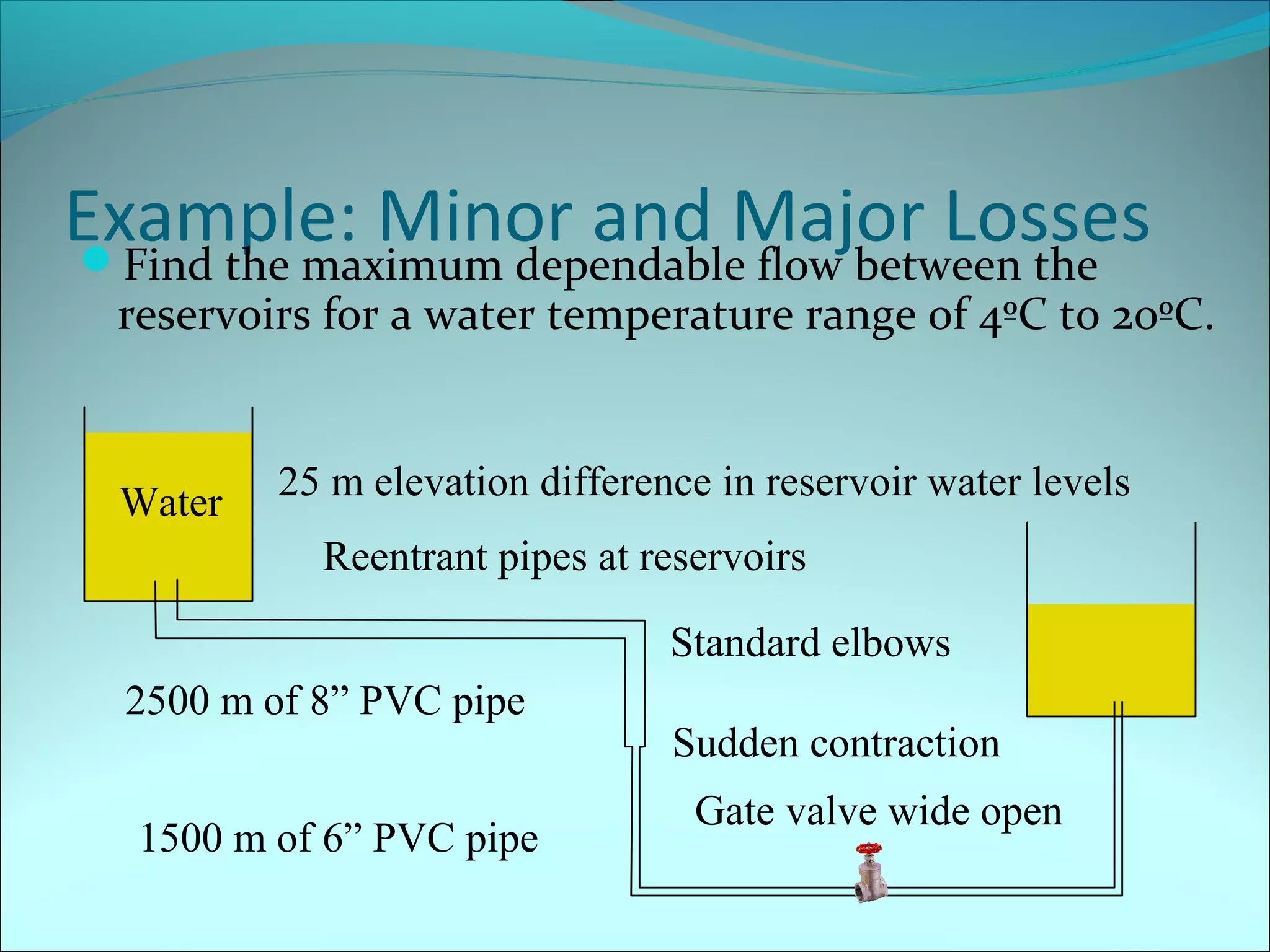


This document provides information on calculating head losses in piping systems. It discusses the use of Bernoulli's equation to relate total head between two points in a piping system. It also covers friction losses using the Darcy-Weisbach equation and the Moody diagram, as well as "minor losses" from fittings, valves, etc. The document presents methods to calculate head loss or flow rate given the other, including iterative techniques. It concludes with an example problem calculating maximum flow between reservoirs considering major and minor losses.


