SOUTHERN CROSS UNIVERSITY School of Business and Tourism MAT10251 Statistical Analysis PROJECT COVER SHEET Please complete all of the following details and then make these sheets the first pages of your project – do not send it as a separate document. Your project must be submitted as a Word document. PART B Student Name: Umair Elahi Student ID No.: 23039692 Tutor’s name: Badri Bhattarai Due date: 13th January 2019 Date submitted: 16Th January 2019 Declaration: I have read and understand the Rules Relating to Awards (Rule 3 Section 18 – Academic Integrity) as contained in the SCU Policy Library. I understand the penalties that apply for academic misconduct and agree to be bound by these rules. The work I am submitting electronically is entirely my own work. . Signed: (please type your name) Umair Date: 16/01/19 STUDENT NAME: Umair Elahi STUDENT ID NUMBER: 23039692 MAT10251 – Statistical Analysis Project Part B Complete the summary table below. Sample Number (last digit of your student ID number) 2 Fuel First letter family name A to M – Unleaded 91 First letter family name N to Z – Diesel E Confidence Level 95% Level of Significance 5% Value: 15% PLEASE ENSURE YOU KEEP A COPY OF YOUR PROJECT Self-Marking Sheet for Part A Reflection/feedback (approximately 200 words) From the work done in part A, the representation of data in a graph was well understood and implemented. As showcased, two graphs were constructed using the same data set but different class intervals resulting in two different shapes. In addition, calculation of the descriptive statistics was well executed. The interpretation of the aforementioned statistical values was also done appropriately with deep understanding of what each statistic meant or represented. However, there were some challenges and mistakes encountered during the tasks. First, the task of introducing data was a challenge. To avoid this in future, taking time to read and fully understand the population from which the sample is derived and also to understand the sample is a step to be taken. By doing so, I will be able to introduce the data before commencing on the calculations. Another challenge was in the choice of the measure of central tendency as the median and mean were close to each other. To avoid this, more background research regarding the same will be done. From the submission and self-marking of part A, I was able to discover the mistakes and challenges I faced when doing the tasks and think of the ways with which I can avoid or rectify such mistakes in the future. Marking and Feedback Sheet Part B Comments: Please follow the provided instruction. If you need any help, please see me next time.Figure 1(Histogram) Similar to Video Bins Midpoints Frequency 134.99 $132.50 6 139.99 $137.50 21 144.99 $142.50 12 149.99 $147.50 16 154.99 $152.50 15 159.99 $157.50 10 164.99 $162.50 0 Figure 2 (Histogram) With New Clases Bins and Midpoints Bins Midpoints.

1. SOUTHERN CROSS UNIVERSITY
School of Business and Tourism
MAT10251 Statistical Analysis
PROJECT COVER SHEET
Please complete all of the following details and then make these
sheets the first pages of your project – do not send it as a
separate document.
Your project must be submitted as a Word document.
PART B
Student Name:
Umair Elahi
Student ID No.:
23039692
Tutor’s name:
Badri Bhattarai
Due date:
13th January 2019
Date submitted:
16Th January 2019
Declaration:
I have read and understand the Rules Relating to Awards (Rule
3 Section 18 – Academic Integrity) as contained in the SCU
Policy Library. I understand the penalties that apply for
academic misconduct and agree to be bound by these rules.
The work I am submitting electronically is entirely my own
work.
.
Signed:
(please type your name)
Umair
Date:

2. 16/01/19
STUDENT NAME: Umair Elahi
STUDENT ID NUMBER: 23039692
MAT10251 – Statistical Analysis
Project Part B
Complete the summary table below.
Sample Number (last digit of your student ID number)
2
Fuel
First letter family name A to M – Unleaded 91
First letter family name N to Z – Diesel
E
Confidence Level
95%
Level of Significance
5%
Value: 15%
PLEASE ENSURE YOU KEEP A COPY OF YOUR PROJECT

3. Self-Marking Sheet for Part A
Reflection/feedback (approximately 200 words)
From the work done in part A, the representation of data in a
graph was well understood and implemented. As showcased,
two graphs were constructed using the same data set but
different class intervals resulting in two different shapes. In
addition, calculation of the descriptive statistics was well
executed. The interpretation of the aforementioned statistical
values was also done appropriately with deep understanding of
what each statistic meant or represented.
However, there were some challenges and mistakes encountered
during the tasks. First, the task of introducing data was a
challenge. To avoid this in future, taking time to read and fully
understand the population from which the sample is derived and
also to understand the sample is a step to be taken. By doing so,
I will be able to introduce the data before commencing on the
calculations. Another challenge was in the choice of the
measure of central tendency as the median and mean were close
to each other. To avoid this, more background research
regarding the same will be done.
From the submission and self-marking of part A, I was able to
discover the mistakes and challenges I faced when doing the
tasks and think of the ways with which I can avoid or rectify
such mistakes in the future.
Marking and Feedback Sheet Part B
Comments: Please follow the provided instruction. If you need
any help, please see me next time.Figure 1(Histogram) Similar
to Video

4. Bins
Midpoints
Frequency
134.99
$132.50
6
139.99
$137.50
21
144.99
$142.50
12
149.99
$147.50
16
154.99
$152.50
15
159.99
$157.50
10
164.99
$162.50
0
Figure 2 (Histogram) With New Clases Bins and Midpoints
Bins
Midpoints

5. Frequency
131.99
$131.00
0
133.99
$133.00
4
135.99
$135.00
9
137.99
$137.00
7
139.99
$139.00
7
141.99
$141.00
4
143.99
$143.00
6
145.99
$145.00
4
147.99
$147.00
6
149.99
$149.00
8
151.99
$151.00
6
153.99
$153.00

6. 7
155.99
$155.00
10
157.99
$157.00
1
159.99
$159.00
1
161.99
$161.00
0
The First and Second graph are construted using the same data
but because of choosing different classes the shapes are
different . The first data set shows a skew to the right while the
second one is showing some sort of symmetric or uniform data
set, the first graph is constructed using 5 cents difference while
the second is costructed using 2 cents difference,
So defining the second one in detail.As you can see that the
above grapgh is representing the NSW Unleaded 91 Fuel prices
in 80 Town/Suburbs according to Cents per litre with different
prices ranging from 132.9 cents / litre the minimum to 158.9
cents / litre the maxium.
Descriptive Summary
Cents Per Litre
Mean
145.3375
Median
145.85

7. Mode
155.9
Minimum
132.9
Maximum
158.9
Range
26
Variance
55.5586
Standard Deviation
7.4538
Coeff. of Variation
5.13%
Skewness
0.0083
Kurtosis
-1.3280
Count
80
Standard Error
0.8334
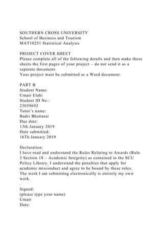
From the above graph we can see that there are four suburbs for
the fuel prices ranging from 130 cents/litre to 134cents/litre,
four for 142cents/litre to 144cents/litre and four for
144cents/litre to 146 cents/litre while majority of the suburbs
has got the same price range i.e. 134 cents/litre to 136
cents/litre and but if we see prices ranging from136 cents/litre
to 138 cents/litre and 138 cents/litre to 140 cents/litre we can
see that seven of the suburbs has got the same price range
respectively.
Descriptive Statistics
More useful information can be found in the descriptive
statistics in the table given above. In particular the least fuel

8. price among all of the suburbs in NSW is 132.9 cents/litre while
the most expensive or highest is 158.9 cents/litre. The median,
which is the middle value among 80 suburbs fuel prices is
145.85 cents/litre i.e. 50 precent of the suburbs are falling
under this price range. While the mean, the single value, the
central tendency, the average is 145.335 cents/litre. As the
mean and median are comparatively same we can conclude that
average fuel price among 80 suburbs is 145.335 cents/litre.
However the standard deviation of 7.4538 shows that the most
of the fuel prices are very very close to the mean i.e. 145.335
cents/litre because of the less standard deviation.
Five-Number Summary
Minimum
132.90
First quartile
137.90
Median
145.85
Third quartile
151.90
Maximum
158.90
Furthermore we will end up by describing the five numbers
summary given above which divides the samples into quarters,
with 25% of the data set in the sample lie below the first
quartile i.e. 137.90 cents/litre and 25% more lie above the third
quartile i.e. 151.90 cents/litre.
Figure 3 Boxplot

9. Written Answer Part B Components of a longer report
The questions in part B both deal with the question of whether
or not motorists view the price of the fuel as expensive though
from different perspectives.
Question 1 in particular answers the question of whether the
price of the fuel is expensive from the perspective of the
population mean. The sample mean was estimated to be
145.3375 cents.
The results are as follows:
The interval was found to be [143.7074 , 146.9709] cents
Since the interval does not include the value $1.50 or 150 cents,
the null hypothesis is rejected. Comment by Badri Bhattarai:
????? please display your excel output.
Question 2 on the other hand answers the question of whether or
not the fuel price is expensive from the perspective of a subset
(more than 25% of petrol stations)of the sample having the fuel
price at least $1.50 per litre.
Calculations were done and the results are as follows:
It was found that the price of fuel in 24 out of 80 petrol stations
in the state was higher than $1.50. This translates to 30%.
B.1 Average Price Unleaded 91/Diesel Price
No, the average price of fuel on that day and in the state
specified was not expensive. This is so since as per the interval
test in statistics that was carried out (check appendix), the null
hypothesis which states that the fuel was expensive was rejected
in our case.
B.2 Unleaded 91/Diesel Price Expensive
Yes, the price of fuel was at least $1.50 per litre in more than
25% of petrol stations in the state specified by the sample.

10. From the foregoing, we conclude that using the criteria where
motorists perceive fuel price to be expensive when the price of
fuel is at least $1.50 at more than 25% petrol stations in a state,
the price of the fuel was expensive on the day in the state
specified. Comment by Badri Bhattarai: Support your answers
with your excel outputs
Appendices Part B
Appendix B.1 – Statistical answer for Question 1
The random variables were defined as follows:
· X_ is a random variable representing the sample mean.
· Sigma represents the standard deviation of the data from the
mean.
· N represents the number of entries or petrol stations in the
sample.
The following assumptions were made in the calculation and
inference of the data:
X ~ N(X_ , Sigma2) i.e. X follows a normal distribution with
mean= X_ and variance Sigma2.
The interval test was chosen in this case. This is because with
the descriptive statistics that were previously calculated it was
easier and faster to use the interval method. Also, the interval
method does not require much calculation in the event that the
average for which the price of fuel has to be to be considered
expensive changes from $1.50. in fact, all that will be needed is
to check whether the new average falls in the interval or not and
make a decision.
Hypothesis testing
Null hypothesis: The price of fuel is expensive. In other words,
the average price is at least $1.50.
Alternative hypothesis: The price of fuel is not expensive. In
other words, the average price is less than $1.50.
To test the above hypothesis, a confidence interval was
constructed as shown below:

11. X_ ± sigma/ where X_= 145.3375 cents, sigma= 7.4538 and
N=80
The 95% confidence interval was found to be [143.7074,
146.9709] cents.
When comparing the value 150 cents to the interval, it can be
seen that the value falls outside the interval on the upper limit.
Therefore, the null hypothesis is rejected.
For question 1, the excel output used was that of the descriptive
statistics that are needed in the calculation of the interval.
Descriptive Summary
Cents Per Litre
Mean
145.3375
Median
145.85
Mode
155.9
Minimum
132.9
Maximum
158.9
Standard Deviation
7.4538
Interpretation of results: since we have failed to reject the null
hypothesis, we conclude that the price of fuel is not expensive
as per the criterion used in question 1.
Appendix B.2 – Statistical answer for Question 2
For question two, only one random variable was defined. X
represents the individual price of fuel at each petrol station in
the state.
The following logical function was used in excel:

12. =IF(C2:C81>150,1,0) where the column C contained the price
of fuel at each petrol station in cents. The column created by
this logical function was then summed to find out the total
number of stations which had at least a fuel price of 150 cents.
Hypothesis testing
Null hypothesis: the percentage of petrol stations with fuel
price higher than 250 cents is greater than 25% hence fuel price
is expensive.
Alternative hypothesis: the percentage of petrol stations with
fuel price less than 250 cents is less than 25% hence fuel price
is not expensive. Comment by Badri Bhattarai: ???
It was found had 24 petrol stations had fuel price higher than
150 cents. This translates to 30%. Therefore, we fail to reject
the null hypothesis.
Interpretation of results: since we have failed to reject the null
hypothesis, we conclude that the price of fuel is expensive as
per the criterion used in question 2. The excel output is as
shown below:
Town/Suburb
Location
Unleaded 91 (Cents per Litre)
logic
Albury
Regional
143.8
0.0
Bathurst
Regional
150.9
1.0
Bermagui
Regional
151.9
1.0
Bourke
Regional

13. 155.9
1.0
Broken Hill
Regional
147.9
0.0
Casino
Regional
155.9
1.0
Coffs Harbour
Regional
153.9
1.0
Coonabarabran
Regional
153.9
1.0
Dorrigo
Regional
148.9
0.0
Drake
Regional
139.9
0.0
Evans Head
Regional
152.9
1.0
Glen Innes
Regional
152.9
1.0
Goulburn
Regional

14. 145.8
0.0
Gunnedah
Regional
142.9
0.0
Halfway Creek
Regional
155.9
1.0
Kempsey
Regional
146.9
0.0
Lismore
Regional
155.9
1.0
Manilla
Regional
156.9
1.0
Moree
Regional
152.9
1.0
Mudgee
Regional
155.9
1.0
Mungindi
Regional
155.9
1.0
Muswellbrook
Regional

15. 158.9
1.0
Narrabri
Regional
149.9
0.0
Newcastle West
Regional
154.9
1.0
Port Kembla
Regional
138.9
0.0
Port Macquarie
Regional
155.4
1.0
Queanbeyan
Regional
149.9
0.0
Tamworth
Regional
149.9
0.0
Tenterfield
Regional
146.7
0.0
Tenterfield
Regional
146.7
0.0
Tweed Heads
Regional

16. 148.9
0.0
Ulladulla
Regional
144.7
0.0
Uralla
Regional
151.9
1.0
Waga Waga
Regional
154.9
1.0
Walgett
Regional
150.9
1.0
Wauchope
Regional
155.9
1.0
West Armidale
Regional
151.0
1.0
Woolgoolga
Regional
153.9
1.0
Wyong
Regional
141.7
0.0
Yamba
Regional

17. 153.9
1.0
Alexandria
Capital - Sydney
143.9
0.0
Arncliffe
Capital - Sydney
136.9
0.0
Bankstown
Capital - Sydney
133.9
0.0
Baulkham Hills
Capital - Sydney
141.9
0.0
Bexley North
Capital - Sydney
135.9
0.0
Blacktown
Capital - Sydney
136.9
0.0
Bondi Junction
Capital - Sydney
148.4
0.0
Brighton Le Sands
Capital - Sydney
135.9
0.0
Brookvale
Capital - Sydney

18. 146.4
0.0
Cabramatta
Capital - Sydney
142.9
0.0
Casula
Capital - Sydney
137.9
0.0
Croydon Park
Capital - Sydney
135.7
0.0
Fairfield
Capital - Sydney
135.9
0.0
Five Dock
Capital - Sydney
150.0
0.0
Forestville
Capital - Sydney
149.4
0.0
Granville
Capital - Sydney
132.9
0.0
Homebush
Capital - Sydney
135.8
0.0
Leppington
Capital - Sydney

19. 135.9
0.0
Lewisham
Capital - Sydney
133.9
0.0
Lidcombe
Capital - Sydney
138.9
0.0
Maroubra
Capital - Sydney
143.9
0.0
Marrickville
Capital - Sydney
137.5
0.0
Miranda
Capital - Sydney
137.9
0.0
Mona Vale
Capital - Sydney
144.9
0.0
Mortdale
Capital - Sydney
136.9
0.0
North Ryde
Capital - Sydney
135.9
0.0
Northwood
Capital - Sydney

20. 139.9
0.0
Pagewood
Capital - Sydney
148.4
0.0
Pennant Hills
Capital - Sydney
143.4
0.0
Petersham
Capital - Sydney
137.7
0.0
Punchbowl
Capital - Sydney
138.9
0.0
Quakers Hill
Capital - Sydney
139.9
0.0
Revesby
Capital - Sydney
133.9
0.0
Ryde
Capital - Sydney
140.9
0.0
Sydney
Capital - Sydney
138.7
0.0
Tarren Point
Capital - Sydney

21. 140.4
0.0
Villawood
Capital - Sydney
134.7
0.0
West Hoxton
Capital - Sydney
145.9
0.0
Woolloomooloo
Capital - Sydney
146.9
0.0
Yagoona
Capital - Sydney
134.5
0.0
24.0
Do not cut my marks as I have been approved by my unit
assessor because I have got the extension but I can’t be able to
upload my assignment again thill the extension date so she reset
my link. The attached copy of email you can see below thanks.
2

22. Sheet1Max MarksRecommended MarksCover sheet or sample
incorrect-2.0Format incorrect, including name-2.0Statistical
CalculationsGraph (Frequency Histogram or
Polygon)4.04.0Descriptive Statistics4.04.0Total Descriptive
Statistics8.08.0Written Answer (Component of a business
report)Introduction and data2.00.0Comments on
graph3.03.0`Comments on descriptive statistics4.03.0Difference
in measures of central tendency1.01.0Structure, grammar and
spelling2.02.0Total Report12.09.0Total20.017.0
Sheet2
Sheet3
Max MarksMark
Cover sheet or sample incorrect-2
Format incorrect, including file name-2
Self-Marking and Reflection Part A (5 marks)
Self-Marking Part A22.0
Reflection32.0
Part B Statistical Inference Tasks (19 marks)
Statistical Inference Question 1
Choice of technique, assumptions & other required steps41.0
Calculation (Excel output)30.0
Conclusion20.0
Statistical Inference Question 2
Choice of technique, assumptions & other required steps50.0
Calculation (Excel output)30.0
Decision and conclusion20.0
Written task - Discussion and results (6 marks)
Question 121.0
Question 220.0
Structure, grammar and spelling21.0
Total Part B307.0
Sheet1Max MarksMarkCover sheet or sample incorrect-2Format
incorrect, including file name-2Self-Marking and Reflection
Part A (5 marks)Self-Marking Part A22.0Reflection32.0Part B
Statistical Inference Tasks (19 marks)Statistical Inference
Question 1 Choice of technique, assumptions & other required

23. steps41.0Calculation (Excel
output)30.0Conclusion20.0Statistical Inference Question
2Choice of technique, assumptions & other required
steps50.0Calculation (Excel output)30.0Decision and
conclusion20.0Written task - Discussion and results (6
marks)Question 121.0Question 220.0Structure, grammar and
spelling21.0Total Part B307.0
Sheet2
Sheet3
Max MarksRecommended
Marks
Cover sheet or sample incorrect-2.0
Format incorrect, including name-2.0
Statistical Calculations
Graph (Frequency Histogram or Polygon)4.04.0
Descriptive Statistics4.04.0
Total Descriptive Statistics8.08.0
Written Answer (Component of a business
report)
Introduction and data2.00.0
Comments on graph3.03.0
Comments on descriptive statistics4.03.0
Difference in measures of central tendency1.01.0
Structure, grammar and spelling2.02.0
Total Report12.09.0
Total20.017.0
SOUTHERN CROSS UNIVERSITY
School of Business and Tourism
MAT10251 Statistical Analysis
PROJECT COVER SHEET
Please complete all of the following details and then make these
sheets the first pages of your project – do not send it as a
separate document.
Your project must be submitted as a Word document.

24. PART B
Student Name:
Student ID No.:
Tutor’s name:
Due date:
Date submitted:
Declaration:
I have read and understand the Rules Relating to Awards (Rule
3 Section 18 – Academic Integrity) as contained in the SCU
Policy Library. I understand the penalties that apply for
academic misconduct and agree to be bound by these rules.
The work I am submitting electronically is entirely my own
work.
Signed:
(please type your name)
Date:
STUDENT NAME:
STUDENT ID NUMBER:
MAT10251 – Statistical Analysis

25. Project Part B
Complete the summary table below.
Sample Number (last digit of your student ID number)
Fuel
First letter family name A to M – Unleaded 91
First letter family name N to Z – Diesel
Confidence Level
Level of Significance
Value: 15%
PLEASE ENSURE YOU KEEP A COPY OF YOUR PROJECT
Self-Marking Sheet for Part A
Reflection/feedback (approximately 200 words)
Marking and Feedback Sheet Part B

26. Comments
The written task and appendices should appear here after a copy
of your Part A submission
Delete the italic text and add your contentWritten Answer Part
B Components of a longer report
Each answer below should:
· Introduce and put the question in context
· Include appropriate Excel output.
· Present the results of your intervals or tests without
unnecessary statistical jargon.
ResultsB.1 Average Price Unleaded 91/Diesel Price
100 to 200 words and 0.5 to 1.5 pages
Use the estimate, constructed in Question 1, for the population
mean price of your fuel on the day and in the state specified by
your sample, to provide a justified answer to the question
Was the average price of your fuel expensive on the day and in
the state specified by your sample?
B.2 Unleaded 91/Diesel Price Expensive
100 to 200 words and 0.5 to 1.5 pages
Use your answer to Question 2:
On the specified day was the price of your fuel at least $1.50
per litre in more than 25% of petrol stations in the state
specified by your sample?
to decide if the price of your fuel was expensive on the day and
in the state specified by your sample.
Appendices Part B
The appendices should show full statistical working for each
question and should include

27. · Definition of random variable/s
· Any required assumptions.
· Why test or interval was chosen
· Hypotheses and decision for a hypothesis test
· Excel output
· Interpretation of results and a conclusion
Appendix B.1 – Statistical answer for Question 1
Estimate the population mean price of your fuel, Unleaded 91 or
Diesel, on the day and in the state specified by your sample.
Appendix B.2 – Statistical answer for Question 2
On the specified day was the price of your fuel at least $1.50
per litre in more than 25% of petrol stations in the state
specified by your sample?
6
Max MarksMark
Cover sheet or sample incorrect-2
Format incorrect, including file name-2
Self-Marking and Reflection Part A (5 marks)
Self-Marking Part A2
Reflection3
Part B Statistical Inference Tasks (19 marks)
Statistical Inference Question 1
Choice of technique, assumptions & other required steps4
Calculation (Excel output)3
Conclusion2
Statistical Inference Question 2
Choice of technique, assumptions & other required steps5
Calculation (Excel output)3
Decision and conclusion2
Written task - Discussion and results (6 marks)

28. Question 12
Question 22
Structure, grammar and spelling2
Total Part B300.0
Sheet1Max MarksMarkCover sheet or sample incorrect-2Format
incorrect, including file name-2Self-Marking and Reflection
Part A (5 marks)Self-Marking Part A2Reflection3Part B
Statistical Inference Tasks (19 marks)Statistical Inference
Question 1 Choice of technique, assumptions & other required
steps4Calculation (Excel output)3Conclusion2Statistical
Inference Question 2Choice of technique, assumptions & other
required steps5Calculation (Excel output)3Decision and
conclusion2Written task - Discussion and results (6
marks)Question 12Question 22Structure, grammar and
spelling2Total Part B300.0
Sheet2
Sheet3
Max Marks
Recommended
Marks
Cover sheet or sample incorrect-2.0
Format incorrect, including name-2.0
Statistical Calculations
Graph (Frequency Histogram or Polygon)4.0
Descriptive Statistics4.0
Total Descriptive Statistics8.0
0.0
Written Answer (Component of a business
report)
Introduction and data2.0
Comments on graph3.0
Comments on descriptive statistics4.0
Difference in measures of central tendency1.0
Structure, grammar and spelling2.0
Total Report12.0
0.0

29. Total20.0
0.0
Sheet1Max MarksRecommended MarksCover sheet or sample
incorrect-2.0Format incorrect, including name-2.0Statistical
CalculationsGraph (Frequency Histogram or
Polygon)4.0Descriptive Statistics4.0Total Descriptive
Statistics8.00.0Written Answer (Component of a business
report)Introduction and data2.0Comments on
graph3.0`Comments on descriptive statistics4.0Difference in
measures of central tendency1.0Structure, grammar and
spelling2.0Total Report12.00.0Total20.00.0
Sheet2
Sheet3
Sheet1Max MarksRecommended MarksCover sheet or sample
incorrect-2.0Format incorrect, including name-2.0Statistical
CalculationsGraph (Frequency Histogram or
Polygon)4.0Descriptive Statistics4.0Total Descriptive
Statistics8.00.0Written Answer (Component of a business
report)Introduction and data2.0Comments on
graph3.0Comments on descriptive statistics4.0Difference in
measures of central tendency1.0Structure, grammar and
spelling2.0Total Report12.00.0Total20.00.0
MAT10251 Workbooks 2018/~$Multiple Regression 2
Independent Variables Workbook.xlsx
MAT10251 Workbooks 2018/~$Simple Linear Regression
Workbook.xlsx
MAT10251 Workbooks 2018/Boxplot Workbook.xlsx
DATAFestival ExpenditureAmount Spent
$11196159715533435029281005993408725763
Boxplot

30. Festival Expenditure
343 343 343 0.5 1 1.5 502 502 502 0.5 1 1.5
744 744 744 0.5 1 1.5 993 993 993 0.5 1
1.5 1119 1119 1119 0.5 1 1.5 343 1119 1 1
502 993 0.5 0.5 502 993 1.5 1.5 Amount Spent $
Five-Number SummaryFive-Number
SummaryMinimum343.00First
quartile502.00Median744.00Third
quartile993.00Maximum1119.00
PLOT_DATAFive-Number
SummaryMinimum343.00ValuePlotFirst
quartile502.003430.5Median744.003431Third
quartile993.003431.5Maximum1119.005020.550215021.57440.5
74417441.59930.599319931.511190.51119111191.53431111915
020.59930.55021.59931.5Quartile Calculations (Book
Rules)Initial first quartile rank3.25Rule 3 appliesuse
rank:3value of rank:502first quartile:502Initial third quartile
rank9.75Rule 3 appliesuse rank:10value of rank:993third
quartile:993
PLOT_SUMMARYFive-Number
SummaryMinimum343.00ValuePlotFirst
quartile502.003430.5Median744.003431Third
quartile993.003431.5Maximum1119.005020.550215021.57440.5
74417441.59930.599319931.511190.51119111191.53431111915
020.59930.55021.59931.5
Boxplot

31. 343 343 343 0.5 1 1.5 502 502 502 0.5 1 1.5
744 744 744 0.5 1 1.5 993 993 993 0.5 1
1.5 1119 1119 1119 0.5 1 1.5 343 1119 1 1
502 993 0.5 0.5 502 993 1.5 1.5
PLOT_DATA_FORMULASFive-Number
SummaryMinimum343.00ValuePlotFirst
quartile502.003430.5Median744.003431Third
quartile993.003431.5Maximum1119.005020.550215021.57440.5
74417441.59930.599319931.511190.51119111191.53431111915
020.59930.55021.59931.5Quartile Calculations (Book
Rules)Initial first quartile rank3.25Rule 3 appliesuse
rank:3value of rank:502first quartile:502Initial third quartile
rank9.75Rule 3 appliesuse rank:10value of rank:993third
quartile:993
Boxplot
343 343 343 0.5 1 1.5 502 502 502 0.5 1 1.5
744 744 744 0.5 1 1.5 993 993 993 0.5 1
1.5 1119 1119 1119 0.5 1 1.5 343 1119 1 1
502 993 0.5 0.5 502 993 1.5 1.5
PLOT_FORMULASFive-Number
SummaryMinimum343.00ValuePlotFirst
quartile502.003430.5Median744.003431Third
quartile993.003431.5Maximum1119.005020.550215021.57440.5
74417441.59930.599319931.511190.51119111191.53431111915
020.59930.55021.59931.5

32. Boxplot
343 343 343 0.5 1 1.5 502 502 502 0.5 1 1.5
744 744 744 0.5 1 1.5 993 993 993 0.5 1
1.5 1119 1119 1119 0.5 1 1.5 343 1119 1 1
502 993 0.5 0.5 502 993 1.5 1.5
MAT10251 Workbooks 2018/CIE Proportion Workbook.xlsx
COMPUTEConfidence Interval: Proportion DataSample
Size100Number of Successes10Confidence
Level95%Intermediate CalculationsSample Proportion0.1Z
Value-1.9600Standard Error of the Proportion0.03Interval Half
Width0.0588Confidence IntervalInterval Lower
Limit0.0412Interval Upper Limit0.1588
COMPUTE_FORMULASConfidence Interval: Proportion
DataSample Size100Number of Successes10Confidence
Level95%Intermediate CalculationsSample Proportion0.1Z
Value-1.9600Standard Error of the Proportion0.03Interval Half
Width0.0588Confidence IntervalInterval Lower
Limit0.0412Interval Upper Limit0.1588
COMPUTE_OLDERConfidence Interval: Proportion
DataSample Size100Number of Successes10Confidence
Level95%Intermediate CalculationsSample Proportion0.1Z
Value-1.9600Standard Error of the Proportion0.03Interval Half
Width0.0588Confidence IntervalInterval Lower
Limit0.0412Interval Upper Limit0.1588
COMPUTE_OLDER_FORMULASConfidence Interval:
Proportion DataSample Size100Number of
Successes10Confidence Level95%Intermediate
CalculationsSample Proportion0.1Z Value-1.9600Standard Error
of the Proportion0.03Interval Half Width0.0588Confidence

33. IntervalInterval Lower Limit0.0412Interval Upper Limit0.1588
MAT10251 Workbooks 2018/CIE Sigma Known Workbook.xlsx
DATAExam
Mark47.8038.1057.2042.4568.2579.3518.3050.6547.6052.0051.
6567.8071.3055.7555.4576.4059.8076.1586.2086.3564.5587.10
83.4557.6579.9051.6553.8018.7551.0552.15
COMPUTE POP SDConfidence Estimate for the
MeanDataPopulation Standard Deviation17.90022Sample
Mean59.62Sample Size30Confidence Level95%Intermediate
CalculationsStandard Error of the Mean3.2681180928Z Value-
1.9600Interval Half Width6.4054Confidence IntervalInterval
Lower Limit53.2146Interval Upper Limit66.0254
COMPUTE SAMPLE SDConfidence Estimate for the
MeanDataSample Standard Deviation17.9002196095Sample
Mean59.62Sample Size30Confidence Level95%Intermediate
CalculationsStandard Error of the Mean3.2681180215Z Value-
1.9600Interval Half Width6.4054Confidence IntervalInterval
Lower Limit53.2146Interval Upper Limit66.0254
COMPUTE STATISTICSConfidence Estimate for the
MeanDataPopulation/Sample Standard
Deviation17.9002196095Sample Mean59.62Sample
Size30Confidence Level95%Intermediate CalculationsStandard
Error of the Mean3.2681180215Z Value-1.9600Interval Half
Width6.4054Confidence IntervalInterval Lower
Limit53.2146Interval Upper Limit66.0254
COMPUTE_FORMULASConfidence Estimate for the
MeanDataPopulation Standard Deviation17.9002Sample
Mean59.62Sample Size30Confidence Level95%Intermediate
CalculationsStandard Error of the Mean3.2681144413Z Value-
1.9600Interval Half Width6.4054Confidence IntervalInterval
Lower Limit53.2146Interval Upper Limit66.0254
COMPUTE_OLDERConfidence Estimate for the
MeanDataPopulation Standard Deviation17.9002Sample
Mean59.62Sample Size30Confidence Level95%Intermediate
CalculationsStandard Error of the Mean3.2681144413Z Value-

34. 1.9600Interval Half Width6.4054Confidence IntervalInterval
Lower Limit53.2146Interval Upper Limit66.0254
COMPUTE_OLDER_FORMULASConfidence Estimate for the
MeanDataPopulation Standard Deviation17.9002Sample
Mean59.62Sample Size30Confidence Level95%Intermediate
CalculationsStandard Error of the Mean3.2681144413Z Value-
1.9600Interval Half Width6.4054Confidence IntervalInterval
Lower Limit53.2146Interval Upper Limit66.0254
MAT10251 Workbooks 2018/CIE Sigma Unknown
Workbook.xlsx
DATAExam
Mark47.8038.1057.2042.4568.2579.3518.3050.6547.6052.0051.
6567.8071.3055.7555.4576.4059.8076.1586.2086.3564.5587.10
83.4557.6579.9051.6553.8018.7551.0552.15
COMPUTEConfidence Estimate for the MeanDataSample
Standard Deviation17.9002196095Sample Mean59.62Sample
Size30Confidence Level95%Intermediate CalculationsStandard
Error of the Mean3.2681Degrees of Freedom29t
Value2.0452Interval Half Width6.6841Confidence
IntervalInterval Lower Limit52.94Interval Upper Limit66.30
COMPUTE_STATISTICSConfidence Estimate for the
MeanDataSample Standard Deviation17.9002196095Sample
Mean59.62Sample Size30Confidence Level95%Intermediate
CalculationsStandard Error of the Mean3.2681Degrees of
Freedom29t Value2.0452Interval Half Width6.6841Confidence
IntervalInterval Lower Limit52.94Interval Upper Limit66.30
COMPUTE_FORMULASConfidence Estimate for the
MeanDataSample Standard Deviation17.9002196095Sample
Mean59.62Sample Size30Confidence Level95%Intermediate
CalculationsStandard Error of the Mean3.2681Degrees of
Freedom29t Value2.0452Interval Half Width6.6841Confidence
IntervalInterval Lower Limit52.94Interval Upper Limit66.30
COMPUTE_OLDERConfidence Estimate for the
MeanDataSample Standard Deviation17.9002196095Sample
Mean59.62Sample Size30Confidence Level95%Intermediate

35. CalculationsStandard Error of the Mean3.2681Degrees of
Freedom29t Value2.0452Interval Half Width6.6841Confidence
IntervalInterval Lower Limit52.94Interval Upper Limit66.30
COMPUTE_OLDER_FORMULASConfidence Estimate for the
MeanDataSample Standard Deviation17.9002196095Sample
Mean59.62Sample Size30Confidence Level95%Intermediate
CalculationsStandard Error of the Mean3.2681Degrees of
Freedom29t Value2.0452Interval Half Width6.6841Confidence
IntervalInterval Lower Limit52.94Interval Upper Limit66.30
MAT10251 Workbooks 2018/Descriptive Statistics
Workbook.xlsx
DATAGet-Ready Time39294352394440314435
Descriptive_SummaryDescriptive SummaryGet-Ready
TimeMean39.6Median39.5Mode39Minimum29Maximum52Rang
e23Variance45.8222Standard Deviation6.7692Coeff. of
Variation17.09%Skewness0.0858Kurtosis0.1375Count10Standar
d Error2.1406
ZScoresGet-Ready TimeZ Score39-0.0929-1.57430.50521.8339-
0.09440.65400.0631-1.27440.6535-0.68
Descriptive_Summary_FORMULASDescriptive SummaryGet-
Ready
TimeMean39.6Median39.5Mode39Minimum29Maximum52Rang
e23Variance45.8222Standard Deviation6.7692Coeff. of
Variation17.09%Skewness0.0858Kurtosis0.1375Count10Standar
d Error2.1406
Descriptive_Summary_OLDERDescriptive SummaryGet-Ready
TimeMean39.6Median39.5Mode39Minimum29Maximum52Rang
e23Variance45.8222Standard Deviation6.7692Coeff. of
Variation17.09%Skewness0.0858Kurtosis0.1375Count10Standar
d Error2.1406
Descriptive_Summary_OLD_FORMULDescriptive
SummaryGet-Ready
TimeMean39.6Median39.5Mode39Minimum29Maximum52Rang
e23Variance45.8222Standard Deviation6.7692Coeff. of
Variation17.09%Skewness0.0858Kurtosis0.1375Count10Standar

36. d Error2.1406
MAT10251 Workbooks 2018/Exponential Smoothing
Workbook.xlsx
Chart1
Sales (Yi) 1 2 3 4 5 6 7 8 9 10 11
23 40 25 27 32 48 33 37 37 50 40
0.2 1 2 3 4 5 6 7 8 9 10 11
23 26.400000000000002 26.120000000000005
26.296000000000006 27.436800000000005
31.549440000000008 31.839552000000008
32.871641600000011 33.69731328000001
36.95785062400001 37.566280499200005 0.25 1 2
3 4 5 6 7 8 9 10 11 23 27.25
26.6875 26.765625 28.07421875 33.0556640625
33.041748046875 34.03131103515625
34.773483276367188 38.580112457275391
38.935084342956543 Time Period (i)
Sales (Yi)
COMPUTEWWAdd or delete rows rows 5 to 10Time Period
(i)Sales (Yi)0.20.25then copy formulas from row 4 in columns
C and
D12323.0023.0024026.4027.2532526.1226.6942726.3026.77532
27.4428.0764831.5533.0673331.8433.0483732.8734.0393733.70
34.77105036.9638.58114037.5738.94
MAT10251 Workbooks 2018/Histogram Workbook Use When
Have Zero in Data.xlsx
DataSuburban RestaurantPrice of Main Meal $Bin
ValuesMidpoint
ValuesMinimum233719.999$17.50Maximum553724.999$22.50

37. Range322929.999$27.503834.999$32.503739.999$37.503844.99
9$42.503949.999$47.502954.999$52.503659.999$57.503864.99
9$62.504469.999$67.502774.999$72.502479.999$77.503484.99
9$82.504489.999$87.50233032252943312634234132302833265
1264839552438313051302738262833383225
Histogram and
FrequencyBinsMidpointsFrequency19.999$17.50024.999$22.50
429.999$27.501334.999$32.501339.999$37.501244.999$42.504
49.999$47.50154.999$52.50259.999$57.50164.999$62.50069.99
9$67.50074.999$72.50079.999$77.50084.999$82.50089.999$87.
500
Suburban Restaurant
Frequency 17.5 22.5 27.5 32.5 37.5 42.5 47.5 52.5 57.5
62.5 67.5 72.5 77.5 82.5 87.5 0 4 13 13 12 4
1 2 1 0 0 0 0 0 0 Price of
Main Meal $
Frequency
MAT10251 Workbooks 2018/Histogram Workbook.xlsx
DataSuburban RestaurantPrice of Main Meal $Bin
ValuesMidpoint
ValuesMinimum23379.999$7.50Maximum553714.999$12.50Ra
nge322919.999$17.503824.999$22.503729.999$27.503834.999$
32.503939.999$37.502944.999$42.503649.999$47.503854.999$
52.504459.999$57.502764.999$62.502434442330322529433126
34234132302833265126483955243831305130273826283338322
5
Histogram

38. Suburban Restaurant
Frequency 12.5 17.5 22.5 27.5 32.5 37.5 42.5 47.5 52.5
57.5 62.5 0 0 4 13 13 12 4 1 2 1
0 Price of Main Meal $
Frequency
FrequencyBinsMidpointsFrequency9.999$7.50014.999$12.5001
9.999$17.50024.999$22.50429.999$27.501334.999$32.501339.9
99$37.501244.999$42.50449.999$47.50154.999$52.50259.999$
57.50164.999$62.5000$0.0000$0.0000$0.0000$0.0000$0.0000$
0.0000$0.0000$0.000
MAT10251 Workbooks 2018/Moving Averages Workbook.xlsx
Chart1
Unemp 1995 1996 1997 1998 1999 2000 2001 2002 2003 2004
2005 2006 2007 258 263 315 247 222 236 317 288
279 288 231 228 219 MA 3-Year 1995 1996 1997
1998 1999 2000 2001 2002 2003 2004 2005 2006 2007 #N/A
278.66666666666669 275 261.33333333333331
235 258.33333333333331 280.33333333333331
302.5 279 259.5 249 226 #N/A MA 5-Year
1995 1996 1997 1998 1999 2000 2001 2002 2003 2004 2005
2006 2007 #N/A #N/A 261 256.60000000000002
267.39999999999998 262 268.39999999999998
281.60000000000002 280.60000000000002 262.8
249 #N/A #N/A MA 7-Year 1995 1996 1997
1998 1999 2000 2001 2002 2003 2004 2005 2006 2007 #N/A

39. #N/A #N/A 265.42857142857144
269.71428571428572 272 268.14285714285717
265.85714285714283 266.71428571428572
264.28571428571428 #N/A #N/A #N/A
Year
Unemp
COMPUTEYearUnempMA 3-YearMA 5-YearMA 7-YearAdd or
delete rows at row
101995258ERROR:#N/AERROR:#N/AERROR:#N/Athen copy
formulas in row 5 down columns C, D and
E1996263278.67ERROR:#N/AERROR:#N/A1997315275.00261.
00ERROR:#N/A1998247261.33256.60265.431999222235.00267
.40269.712000236258.33262.00272.002001317280.33268.40268
.142002288302.50281.60265.862003279279.00280.60266.71200
4288259.50262.80264.292005231249.00249.00ERROR:#N/A20
06228226.00ERROR:#N/AERROR:#N/A2007219ERROR:#N/A
ERROR:#N/AERROR:#N/A
MAT10251 Workbooks 2018/Multiple Regression 2 Independent
Variables Workbook.xlsx
MRDataDependent variableIndependent variablesAdd or delete
middle rows.BarsPricePromotionRows 4 to 354141159200Copy
1's in column
B384215920030561592003519159200422615940046301594003
50715940037541594005000159600512015960040111596005015
15960019161792006751792003636179200322417920022951794
00273017940026181794004421179400411317960037461796003
53217960038251796001096199200761199200208819920082019
92002114199400188219940021591994001602199400335419960

40. 02927199600
RESIDUALSObservationPricePromotionPredicted
BarsResiduals1592003420.30952380954141720.6904761905259
2003420.30952380953842421.69047619053592003420.3095238
0953056-
364.30952380954592003420.3095238095351998.690476190555
94004142.9211309524422683.07886904766594004142.9211309
5244630487.07886904767594004142.92113095243507-
635.92113095248594004142.92113095243754-
388.92113095249596004865.53273809525000134.46726190481
0596004865.53273809525120254.467261904811596004865.532
73809524011-
854.532738095212596004865.53273809525015149.4672619048
13792002355.9627976191916-
439.96279761914792002355.962797619675-
1680.96279761915792002355.96279761936361280.0372023811
6792002355.9627976193224868.03720238117794003078.57440
476192295-783.574404761918794003078.57440476192730-
348.574404761919794003078.57440476192618-
460.574404761920794003078.574404761944211342.425595238
121796003801.18601190484113311.813988095222796003801.1
8601190483746-55.186011904823796003801.18601190483532-
269.186011904824796003801.1860119048382523.81398809522
5992001291.61607142861096-
195.616071428626992001291.6160714286761-
530.616071428627992001291.61607142862088796.3839285714
28992001291.6160714286820-
471.616071428629994002014.2276785714211499.77232142863
0994002014.22767857141882-
132.227678571431994002014.22767857142159144.7723214286
32994002014.22767857141602-
412.227678571433996002736.83928571433354617.1607142857
34996002736.83928571432927190.1607142857
COMPUTEMultiple RegressionCalculationsb2, b1, b0
intercepts3.6131-53.21735837.5208Regression Statisticsb2, b1,
b0 Standard Error0.68526.8522628.1502Multiple R0.8705R

41. Square, Standard Error0.7577638.0653ERROR:#N/AR
Square0.7577F, Residual df48.477131ERROR:#N/AAdjusted R
Square0.7421Regression SS, Residual
SS39472730.773021712620946.6681548ERROR:#N/AStandard
Error638.0653Observations34Confidence level95%t Critical
Value2.0395ANOVAHalf Width
b01281.1208dfSSMSFSignificance FHalf Width
b113.9752Regression239472730.773019736365.386548.47710.0
000Half Width
b21.3975Residual3112620946.6682407127.3119Total33520936
77.4412CoefficientsStandard Errort StatP-valueLower
95%Upper 95%Lower 95%Upper
95%Intercept5837.5208628.15029.29320.00004556.39997118.6
4164556.39997118.6416Price-53.21736.8522-7.76640.0000-
67.1925-39.2421-67.1925-
39.2421Promotion3.61310.68525.27280.00002.21555.01062.215
55.0106
CIEandPIConfidence Interval Estimate and Prediction
IntervalDataConfidence
Level95%1Price79Promotion400X'X3426461320026462146741
0188001320010188006000000Inverse of X'X0.9692-0.0094-
0.0005-0.00940.00010.0000-0.00050.00000.0000X'G times
Inverse of X'X0.01210.00010.0000[X'G times Inverse of X'X]
times XG0.0298t Statistic2.0395Predicted Y (YHat)3078.57For
Average Predicted Y (YHat)Interval Half
Width224.50Confidence Interval Lower
Limit2854.07Confidence Interval Upper Limit3303.08For
Individual Response YInterval Half Width1320.57Prediction
Interval Lower Limit1758.01Prediction Interval Upper
Limit4399.14
MAT10251 Workbooks 2018/Multiple Regression 3 Independent
Variables Workbook.xlsx
MRDataDependent variableIndependent variablesAdd or delete
middle rows.PriceAgeKms (000)StateRows 4 to
1262500012151Copy 1's in column

42. B220001329014999147301895014451150001563011500169101
65001610901000016831110001615519000171100115001774013
50017691104901813311150018130010950191330850019151097
50199607500110190042001121900430011219018000114182190
01161421430011720903200117253025000121512200013290149
99147301895014451150001563011500169101650016109010000
16831110001615519000171100115001774013500176911049018
13311150018130010950191330850019151097501996075001101
90042001121900430011219018000114182190011614214300117
20903200117253025000121512200013290149991473018950144
51150001563011500169101650016109010000168311100016155
19000171100115001774013500176911049018133111500181300
10950191330850019151097501996075001101900420011219004
30011219018000114182190011614214300117209032001172530
25000121512200013290149991473018950144511500015630115
00169101650016109010000168311100016155190001711001150
01774013500176911049018133111500181300109501913308500
19151097501996075001101900420011219004300112190180001
14182190011614214300117209032001172530250001215122000
13290149991473018950144511500015630115001691016500161
09010000168311100016155190001711001150017740135001769
11049018133111500181300109501913308500191510975019960
75001101900420011219004300112190180001141821900116142
14300117209032001172530900116142143001172090320011725
30250011828915501202200
COMPUTEMultiple RegressionCalculationsb2, b1, b0
intercepts-42.7210-28.2782-
818.680021415.024218839Regression Statisticsb2, b1, b0
Standard Error486.32407.7879108.5081575.430985714Multiple
R0.8998R Square, Standard
Error0.80962595.9684ERROR:#N/AERROR:#N/AR
Square0.8096F, Residual
df171.4522121ERROR:#N/AERROR:#N/AAdjusted R
Square0.8048Regression SS, Residual
SS3466275351.3257815425305.474305ERROR:#N/AERROR:#
N/AStandard Error2595.9684Observations125Confidence

43. level95%t Critical Value1.9798ANOVAHalf Width
b01139.2174dfSSMSFSignificance FHalf Width
b1214.8205Regression33466275351.32571155425117.1086171.
45220.0000Half Width
b215.4182Residual121815425305.47436739052.1114Half Width
b3962.8066655651Total1244281700656.8000CoefficientsStanda
rd Errort StatP-valueLower 95%Upper 95%Lower 95%Upper
95%Intercept21415.0242575.431037.21560.000020275.8068225
54.241620275.806822554.2416Age-818.6800108.5081-
7.54490.0000-1033.5005-603.8595-1033.5005-603.8595Kms
(000)-28.27827.7879-3.63100.0004-43.6963-12.8600-43.6963-
12.8600State-42.7210486.3240-0.08780.9301-
1005.5276920.0857-1005.5276920.0857
CI and PIConfidence Interval Estimate and Prediction
IntervalDataConfidence Level95%1Age2Kms
(000)50State0X'X12511081568847110812308169533409156881
695332456650550147409550147Inverse of X'X0.0491346-
0.0012895-0.0001896-0.0157255-0.00128950.0017471-
0.0001100-0.0010385-0.0001896-
0.00011000.00000900.0000935-0.0157255-
0.00103850.00009350.0350956X'G times Inverse of X'X0.0371-
0.0032957290.0000404132-0.0131274565[X'G times Inverse of
X'X] times XG0.0325t Statistic1.9798Predicted Y
(YHat)18363.76For Average Predicted Y (YHat)Interval Half
Width926.61Confidence Interval Lower
Limit17437.15Confidence Interval Upper Limit19290.37For
Individual Response YInterval Half Width5222.27Prediction
Interval Lower Limit13141.49Prediction Interval Upper
Limit23586.02
MAT10251 Workbooks 2018/Multiple Regression 4 Independent
Variables Workbook.xlsx
MRDataDependent variableIndependent variablesAdd or delete
middle rows.Yvar #1var #2var #3var #4Rows 4 to
514139127927162.60Copy 1's in column
B2381126729152.403260130228162.603260128125152.4033451

44. 28428177.812580129219154.903175125539152.4032601316291
62.603118126938154.903317127734167.604082127623170.213
856126830160.013430127828175.304678128229167.603402127
938162.603544128030165.113884128529165.102835128828154
.913799128428157.502495126220165.113232129135152.40300
5128928170.213459129234165.103856126124165.10343012862
2175.313175128226165.103175126626162.603487131422154.9
13941128633165.113544129036149.903430128230165.1035721
29921152.403374128633170.203232127719160.0033451272231
62.603600129536165.103317129022170.203884127741165.103
770129229165.102835126428152.414082128325167.603289127
333167.612126126521165.113912128628172.702807127139175
.303345129321160.002750126624157.504139131928167.60229
6128519160.013118132128167.60
COMPUTEMultiple RegressionCalculationsb4 through b0
intercepts-212.482019.932316.41927.2099388177-
2330.9500260837Regression Statisticsb4 through b0 Standard
Error159.00459.977312.37154.79463961522073.897840347Mult
iple R0.4469R Square, Standard
Error0.1997478.3271ERROR:#N/AERROR:#N/AERROR:#N/A
R Square0.1997F, Residual
df2.807145ERROR:#N/AERROR:#N/AERROR:#N/AAdjusted R
Square0.1286Regression SS, Residual
SS2569028.0810036910295855.1389963ERROR:#N/AERROR:#
N/AERROR:#N/AStandard
Error478.3271Observations50Confidence level95%t Critical
Value2.0141ANOVAHalf Width
b04177.0447dfSSMSFSignificance FHalf Width
b19.6569Regression42569028.0810642257.02032.80710.0366H
alf Width b224.9175Residual4510295855.1390228796.7809Half
Width b320.0954Total4912864883.2200Half Width
b4320.2514CoefficientsStandard Errort StatP-valueLower
95%Upper 95%Intercept-2330.95002073.8978-1.12390.2670-
6507.99471846.0946var #17.20994.79461.50370.1396-
2.447016.8668var #216.419212.37151.32720.1911-
8.498341.3368var #319.93239.97731.99780.0518-

45. 0.163140.0277var #4-212.4820159.0045-1.33630.1882-
532.7334107.7695
CIEandPIConfidence Interval Estimate and Prediction
IntervalDataConfidence Level90%1var #12var #250var #31var
#40X'X501415714138158.5141415740188193996852310317.93
920141339968541551230582.53658158.52310317.9230582.513
33580.912303.71439203652303.714Inverse of X'X18.7985698-
0.0265560382-0.0247432329-0.0645561662-0.095070532-
0.02655600.00010047590.0000355938-
0.00001876360.0005823442-
0.02474320.00003559380.0006689553-
0.00002983590.0022458258-0.0645562-0.0000187636-
0.00002983590.0004350913-0.0010064467-
0.09507050.00058234420.0022458258-
0.00100644670.1105016376X'G times Inverse of X'X17.4437-
0.02459415740.0087458833-0.0656503950.0173790015[X'G
times Inverse of X'X] times XG17.7662t
Statistic1.6794Predicted Y (YHat)-1475.64For Average
Predicted Y (YHat)Interval Half Width3385.97Confidence
Interval Lower Limit-4861.61Confidence Interval Upper
Limit1910.34For Individual Response YInterval Half
Width3479.96Prediction Interval Lower Limit-
4955.60Prediction Interval Upper Limit2004.32
MAT10251 Workbooks 2018/Multiple Regression 5 Independent
Variables Workbook.xlsx
MRDataDependent variableIndependent variablesAdd or delete
middle rows.Yvar #1var #2var #3var #4var #5Rows 4 to
514139127927162.656.250Copy 1's in column
B2381126729152.443.0903260130228162.652.62032601281251
52.442.6403345128428177.865.7712580129219154.956.700317
5125539152.452.1603260131629162.649.9003118126938154.94
6.2703317127734167.663.5004082127623170.258.51138561268
30160.059.8713430127828175.359.8704678128229167.665.770
3402127938162.656.2503544128030165.158.971388412852916
5.149.9002835128828154.948.9913799128428157.550.8002495

46. 126220165.153.5213232129135152.450.8003005128928170.254
.4313459129234165.160.3303856126124165.149.900343012862
2175.358.9713175128226165.155.3403175126626162.655.3403
487131422154.954.8813941128633165.156.7013544129036149.
947.6303430128230165.155.3403572129921152.451.710337412
8633170.262.1403232127719160.048.5303345127223162.651.2
603600129536165.165.7703317129022170.249.9003884127741
165.157.1503770129229165.161.2302835126428152.450.35140
82128325167.663.5003289127333167.658.9712126126521165.1
46.7213912128628172.754.4302807127139175.368.4903345129
321160.046.7202750126624157.549.4404139131928167.665.77
02296128519160.068.0413118132128167.681.650
COMPUTEMultiple RegressionCalculationsb5 through b0
intercepts-210.1841-
1.321520.700516.79391679617.4311787039-
2456.360067457Regression Statisticsb5 through b0 Standard
Error162.259112.566712.456013.00728201845.2850057685241
2.449165389Multiple R0.4471R Square, Standard
Error0.1999483.6713ERROR:#N/AERROR:#N/AERROR:#N/AE
RROR:#N/AR Square0.1999F, Residual
df2.198544ERROR:#N/AERROR:#N/AERROR:#N/AERROR:#
N/AAdjusted R Square0.1090Regression SS, Residual
SS2571615.1061060510293268.1138939ERROR:#N/AERROR:#
N/AERROR:#N/AERROR:#N/AStandard
Error483.6713Observations50Confidence level95%t Critical
Value2.0154ANOVAHalf Width
b04861.9718dfSSMSFSignificance FHalf Width
b110.6512Regression52571615.1061514323.02122.19850.0715
Half Width
b226.2145Residual4410293268.1139233937.9117Half Width
b325.1033Total4912864883.2200Half Width b425.3266Half
Width b5327.0117CoefficientsStandard Errort StatP-valueLower
95%Upper 95%Intercept-2456.36012412.4492-1.01820.3141-
7318.33192405.6118var #17.43125.28501.40610.1667-
3.220118.0824var #216.793913.00731.29110.2034-
9.420543.0084var #320.700512.45601.66190.1036-

47. 4.402845.8039var #4-1.321512.5667-0.10520.9167-
26.648124.0051var #5-210.1841162.2591-1.29540.2020-
537.1958116.8276
CIEandPIConfidence Interval Estimate and Prediction
IntervalDataConfidence Level95%1var #12var #250var #31var
#42var
#50X'X501415714138158.52792.7814141574018819399685231
0317.9792488.453920141339968541551230582.579277.843658
158.52310317.9230582.51333580.91457162.732303.72792.7879
2488.4579277.84457162.73158739.1258794.691439203652303.
7794.6914Inverse of X'X24.8780154-0.0372809837-
0.0429069438-0.10179670770.0640625376-0.2064648572-
0.03728100.00011939610.0000676370.0000469336-
0.00011301480.0007788585-
0.04290690.0000676370.00072322350.0000814286-
0.00019140120.0025786414-
0.10179670.00004693360.00008142860.0006632138-
0.0003924245-0.00032408430.0640625-0.0001130148-
0.0001914012-0.00039242450.000675063-0.0011738246-
0.20646490.00077885850.0025786414-0.0003240843-
0.00117382460.1125427276X'G times Inverse of X'X22.6844-
0.0338394355-0.0069118707-0.0977530440.0552241476-
0.0786468022[X'G times Inverse of X'X] times XG22.2839t
Statistic2.0154Predicted Y (YHat)-1583.74For Average
Predicted Y (YHat)Interval Half Width4601.50Confidence
Interval Lower Limit-6185.25Confidence Interval Upper
Limit3017.76For Individual Response YInterval Half
Width4703.62Prediction Interval Lower Limit-
6287.36Prediction Interval Upper Limit3119.87
MAT10251 Workbooks 2018/Normal Workbook.xlsx
COMPUTENormal ProbabilitiesCommon DataMean7Standard
Deviation2Probability for X <=X Value3.5Z Value-
1.75P(X<=3.5)0.0401Probability for X >X Value9Z
Value1P(X>9)0.1587Probability for X<3.5 or X >9P(X<3.5 or X
>9)0.1987Probability for a RangeFrom X Value5To X Value9Z

48. Value for 5-1Z Value for
91P(X<=5)0.1587P(X<=9)0.8413P(5<=X<=9)0.6827Find X and
Z Given a Cum. Pctage.Cumulative Percentage10.00%Z Value-
1.28X Value4.44Find X Values Given a
PercentagePercentage95.00%Z Value-1.96Lower X
Value3.08Upper X Value10.92
COMPUTE_FORMULASNormal ProbabilitiesCommon
DataMean7Standard Deviation2Probability for X <=X Value7Z
Value0P(X<=7)0.5000Probability for X >X Value9Z
Value1P(X>9)0.1587Probability for X<7 or X >9P(X<7 or X
>9)0.6587Probability for a RangeFrom X Value5To X Value9Z
Value for 5-1Z Value for
91P(X<=5)0.1587P(X<=9)0.8413P(5<=X<=9)0.6827Find X and
Z Values Given Cum. Pctage.Cumulative Percentage10.00%Z
Value-1.28X Value4.44Find X Values Given
PercentagePercentage95.00%Z Value-1.96Lower X
Value3.08Upper X Value10.92
This worksheet makes extensive use of the ampersand operator
(&) to create column A labels dynamically, based on the data
values you enter.
The ampersand allows the construction of a text value. For
example, the cell A10 formula ="P(X<="&B8&")" results in the
display of P(X<=7) because the contents of cell B8, 7, is
combined with "P(X<=" and ")"
COMPUTE_OLDERNormal ProbabilitiesCommon
DataMean7Standard Deviation2Probability for X <=X Value7Z
Value0P(X<=7)0.5Probability for X >X Value9Z
Value1P(X>9)0.1587Probability for X<7 or X >9P(X<7 or X
>9)0.6587Probability for a RangeFrom X Value7To X Value9Z
Value for 70Z Value for
91P(X<=7)0.5000P(X<=9)0.8413P(7<=X<=9)0.3413Find X and
Z Given Cum. Pctage.Cumulative Percentage10.00%Z Value-
1.2815515655X Value4.4368968689
COMPUTE_OLDER_FORMULASNormal ProbabilitiesCommon
DataMean7Standard Deviation2Probability for X <=X Value7Z

49. Value0P(X<=7)0.5Probability for X >X Value9Z
Value1P(X>9)0.1587Probability for X<7 or X >9P(X<7 or X
>9)0.6587Probability for a RangeFrom X Value7To X Value9Z
Value for 70Z Value for
91P(X<=7)0.5000P(X<=9)0.8413P(7<=X<=9)0.3413Find X and
Z Given Cum. Pctage.Cumulative Percentage10.00%Z Value-
1.2815515655X Value4.4368968689
This worksheet makes extensive use of the ampersand operator
(&) to create column A labels dynamically, based on the data
values you enter.
The ampersand allows the construction of a text value. For
example, the cell A10 formula ="P(X<="&B8&")" results in the
display of P(X<=7) because the contents of cell B8, 7, is
combined with "P(X<=" and ")"
MAT10251 Workbooks 2018/One-Way ANOVA Workbook.xlsx
ANOVA 3 GroupsSydneyDarwinCanberra
NJayne: Add or delete rows 3 to 10
12612614613012614713412616514512616715512617316412918
0177136213193141227234171243256179248ANOVA: Single
FactorSUMMARYGroupsCountSumAverageVarianceSydney101
714171.41974.2666666667Darwin101386138.6397.8222222222
Canberra101909190.91487.8777777778ANOVASource of
VariationSSdfMSFP-valueF critBetween
Groups13971.266666666626985.63333333335.42929558980.01
042775363.3541308285Within
Groups34739.7271286.6555555556Total48710.966666666729Le
vel of significance0.05
ANOVA 4 GroupsSydneyMelbourneDarwinCanberra
NJayne: Add or delete rows 3 to 10
12614912614613015412614713415412616514515312616715515

50. 31261731641551291801771701362131931921412272342221712
43256252179248ANOVA: Single
FactorSUMMARYGroupsCountSumAverageVarianceSydney101
714171.41974.2666666667Melbourne101754175.41264.0444444
444Darwin101386138.6397.8222222222Canberra101909190.914
87.8777777778ANOVASource of VariationSSdfMSFP-valueF
critBetween
Groups14504.674999999834834.89166666663.77430225020.01
876107712.8662655509Within
Groups46116.1000000001361281.0027777778Total60620.77499
9999939Level of significance0.05
ANOVA 5 GroupsABCDE
NJayne: Add or delete rows 3 to 6
15168512181776191721101318191615111219191491720171410
14ANOVA: Single
FactorSUMMARYGroupsCountSumAverageVarianceA6108183.
2B610617.66666666673.8666666667C66811.333333333311.866
6666667D65499.2E69215.33333333339.4666666667ANOVASo
urce of VariationSSdfMSFP-valueF critBetween
Groups377.8666666667494.466666666712.56205673760.00000
974372.7587104697Within
Groups188257.52Total565.866666666729Level of
significance0.05
ANOVA 6 Groups ABCDEF
NJayne: Add or delete rows 3 to 6
15161585121817187619172121101318191617151112191920149
17201715141014ANOVA: Single
FactorSUMMARYGroupsCountSumAverageVarianceA6108183.
2B610617.66666666673.8666666667C610617.66666666676.266
6666667D66811.333333333311.8666666667E65499.2F69215.33
333333339.4666666667ANOVASource of VariationSSdfMSFP-
valueF critBetween

51. Groups435.6666666667587.133333333311.91793313070.00000
2092.5335545476Within
Groups219.3333333333307.3111111111Total65535Level of
significance0.05
ANOVA 7 Groups MonTuesWedThurFriSatSun
NJayne: Add or delete rows 3 to 6
135.9130.9134.3141.5139.9138.9137.5134.9128.3132.9140.613
9.9137.9135.9135.9131.9133.9142.9140.9139.2137.9ANOVA:
Single
Factor136.7132.9134.8141.8139.8138.8137.8135.9130.7133.714
0.7139.2138.2136.9SUMMARYGroupsCountSumAverageVarian
ceMon5679.3135.860.408Tues5654.7130.942.948Wed5669.6133
.920.502Thur5707.5141.50.875Fri5699.7139.940.373Sat569313
8.60.285Sun5686137.20.68ANOVASource of
VariationSSdfMSFP-valueF critBetween
Groups394.2434285714665.707238095275.7619282935.262309
18506228E-162.4452593951Within
Groups24.284280.8672857143Total418.527428571434Level of
significance0.05
MAT10251 Workbooks 2018/Paired T Workbook.xlsx
DATASample 1Sample 2Di41000380003000Copy formula in
column C down to calculate differences1800046000-
280002200051000-
2900034000305003500310002800030001100019500-
85002200034000-12000
COMPUTE_ALLPaired t TestDataHypothesized Mean
Diff.0Level of significance0.05Intermediate CalculationsSample
Size7DBar-9714.2857degrees of
freedom6SD14206.3869Standard Error5369.5095t Test Statistic-
1.8092Two-Tail TestOne-Tail CalculationsLower Critical
Value-2.4469T.DIST.RT0.0602Upper Critical Value2.44691 -
T.DIST.RT0.9398p-Value0.1204Do not reject the null
hypothesisLower-Tail TestLower Critical Value-1.9432p-

52. Value0.0602Do not reject the null hypothesisUpper-Tail
TestUpper Critical Value1.9432p-Value0.9398Do not reject the
null hypothesis
CONFIDENCE_INTERVALPaired t TestDataDBar-
9714.2857142857SD14206.3868936274Sample Size7Confidence
Level95.0%Intermediate CalculationsStandard
Error5369.5095356151Degrees of Freedom6t
Value2.4469Interval Half Width13138.7165Confidence
IntervalInterval Lower Limit-22853.0022Interval Upper
Limit3424.4308
COMPUTEPaired t TestDataHypothesized Mean Diff.0Level of
Significance0.05Intermediate CalculationsSample Size7DBar-
9714.2857degrees of freedom6SD14206.3869Standard
Error5369.5095t Test Statistic-1.8092Two-Tailed TestLower
Critical Value-2.4469Upper Critical Value2.4469p-
Value0.1204Do not reject the null hypothesis
COMPUTE_LOWERPaired t TestDataHypothesized Mean
Diff.0Level of significance0.05Intermediate CalculationsSample
Size7DBar-9714.2857degrees of
freedom6SD14206.3869Standard Error5369.5095t Test Statistic-
1.8092Lower-Tail TestOne-Tail CalculationsLower Critical
Value-1.9432T.DIST.RT0.0602p-Value0.06021 -
T.DIST.RT0.9398Do not reject the null hypothesis
COMPUTE_UPPERPaired t TestDataHypothesized Mean
Diff.0Level of significance0.05Intermediate CalculationsSample
Size7DBar-9714.2857degrees of
freedom6SD14206.3869Standard Error5369.5095t Test Statistic-
1.8092Upper-Tail TestOne-Tail CalculationsUpper Critical
Value1.9432T.DIST.RT0.0602p-Value0.93981 -
T.DIST.RT0.9398Do not reject the null hypothesis
COMPUTE_ALL_FORMULASPaired t TestDataHypothesized
Mean Diff.0Level of significance0.05Intermediate
CalculationsSample Size7DBar-9714.2857degrees of
freedom6SD14206.3869Standard Error5369.5095t Test Statistic-
1.8092Two-Tail TestOne-Tail CalculationsLower Critical
Value-2.4469T.DIST.RT0.0602Upper Critical Value2.44691 -

53. T.DIST.RT0.9398p-Value0.1204Do not reject the null
hypothesisLower-Tail TestLower Critical Value-1.9432p-
Value0.0602Do not reject the null hypothesisUpper-Tail
TestUpper Critical Value1.9432p-Value0.9398Do not reject the
null hypothesis
COMPUTE_OLDERPaired t TestDataHypothesized Mean
Diff.0Level of significance0.05Intermediate CalculationsSample
Size7DBar-9714.2857degrees of
freedom6SD14206.3869Standard Error5369.5095t Test Statistic-
1.8092Two-Tail TestOne-Tail CalculationsLower Critical
Value-2.4469TDIST0.0602Upper Critical Value2.44691 -
TDIST0.9398p-Value0.1204Do not reject the null
hypothesisLower-Tail TestLower Critical Value-1.9432p-
Value0.0602Do not reject the null hypothesisUpper-Tail
TestUpper Critical Value1.9432p-Value0.9398Do not reject the
null hypothesis
CONFIDENCE_INTERVAL_OLDERPaired t TestDataDBar-
9714.2857142857SD14206.3868936274Sample Size7Confidence
Level95.0%Intermediate CalculationsStandard
Error5369.5095356151Degrees of Freedom6t
Value2.4469Interval Half Width13138.7165Confidence
IntervalInterval Lower Limit-22853.0022Interval Upper
Limit3424.4308
COMPUTE_OLDER_FORMULASPaired t
TestDataHypothesized Mean Diff.0Level of
significance0.05Intermediate CalculationsSample Size7DBar-
9714.2857degrees of freedom6SD14206.3869Standard
Error5369.5095t Test Statistic-1.8092Two-Tail TestOne-Tail
CalculationsLower Critical Value-2.4469TDIST0.0602Upper
Critical Value2.44691 - TDIST0.9398p-Value0.1204Do not
reject the null hypothesisLower-Tail TestLower Critical Value-
1.9432p-Value0.0602Do not reject the null hypothesisUpper-
Tail TestUpper Critical Value1.9432p-Value0.9398Do not reject
the null hypothesis
DATA_FORMULASSample 1Sample
2Di410003800030001800046000-280002200051000-

54. 2900034000305003500310002800030001100019500-
85002200034000-12000
MAT10251 Workbooks 2018/Parameters Workbook.xlsx
DATAMonthTotal Monthly Road
FatalitiesJanuary107February102March110April114May105June
97July117August112September92October118November106Dece
mber116
COMPUTEPopulation DataParametersTotal Monthly Road
FatalitiesMean108.0000Variance60.6667Standard
Deviation7.7889
COMPUTE_FORMULASPopulation DataParametersTotal
Monthly Road FatalitiesMean108.0000Variance60.6667Standard
Deviation7.7889
COMPUTE_OLDERPopulation DataParametersTotal Monthly
Road FatalitiesMean108.0000Variance60.6667Standard
Deviation7.7889
COMPUTE_OLDER_FORMULASPopulation
DataParametersTotal Monthly Road
FatalitiesMean108.0000Variance60.6667Standard
Deviation7.7889
MAT10251 Workbooks 2018/Polygon Workbook Use When
Zero in Data.xlsx
DataPrice of Main MealCity RestaurantsBin ValuesClass
MidpointsMinimum14509.9997.5Maximum633814.99912.5Rang
e494319.99917.55624.99922.55129.99927.53634.99932.52539.9
9937.53344.99942.54149.99947.54454.99952.53459.99957.5396
4.99962.54969.99967.53774.99972.54079.99977.550503522454
43814445127443950353134484830422635326336385323394537
313953
Frequency, Polygon and OgiveCity
RestaurantsBinsFrequencyPercentageCumulative PctageClass
Midpoints9.99900.00%0.00%7.514.99912.00%2.00%12.519.999
00.00%2.00%17.524.99924.00%6.00%22.529.99936.00%12.00
%27.534.999714.00%26.00%32.539.9991428.00%54.00%37.544

55. .999816.00%70.00%42.549.999510.00%80.00%47.554.999816.0
0%96.00%52.559.99912.00%98.00%57.564.99912.00%100.00%
62.569.99900.00%100.00%67.574.99900.00%100.00%72.579.99
900.00%100.00%77.5
Percentage Polygons
City Restaurants 7.5 12.5 17.5 22.5 27.5 32.5 37.5 42.5
47.5 52.5 57.5 62.5 67.5 72.5 77.5 0 0.02 0 0.04
0.06 0.14000000000000001 0.28000000000000003
0.16 0.1 0.16 0.02 0.02 0 0 0 Price of Main
Meal
Cumulative Percentage
City Restaurants 9.9990000000000006
14.999000000000001 19.999000000000002
24.999000000000002 29.999000000000002
34.999000000000002 39.999000000000002
44.999000000000002 49.999000000000002
54.999000000000002 59.999000000000002
64.998999999999995 69.998999999999995
74.998999999999995 79.998999999999995 0
0.02 0.02 0.06 0.12 0.26 0.54 0.7000000000000000 7
0.8 0.96000000000000008 0.98000000000000009 1
1 1 1 Suburban Restaurants
9.9990000000000006 14.999000000000001
19.999000000000002 24.999000000000002
29.999000000000002 34.999000000000002
39.999000000000002 44.99900000000 0002
49.999000000000002 54.999000000000002

56. 59.999000000000002 64.998999999999995
69.998999999999995 74.998999999999995
79.998999999999995 1 Price of Main Meal
MAT10251 Workbooks 2018/Polygon Workbook.xlsx
DataPrice of Main MealCity RestaurantsSuburban
RestaurantsBin ValuesClass
MidpointsMinimum1450379.9997.5Maximum63383714.99912.5
Range49432919.99917.5563824.99922.5513729.99927.5363834.
99932.5253939.99937.5332944.99942.5413649.99947.5443854.
99952.5344459.99957.5392764.99962.5492469.99967.53734404
45023503035322225452944433831142644345123274144323930
50283533312634514826484830394255262435383231633036513
83053272338392645283733313839325325
Percentage Polygons
Percentage Polygons
City Restaurants 7.5 12.5 17.5 22.5 27.5 32.5 37.5 42.5
47.5 52.5 57.5 62.5 67.5 0 0.02 0 0.04 0.06
0.14000000000000001 0.28000000000000003 0.16
0.1 0.16 0.02 0.02 0 Suburban Restaurants 0 0
0.08 0.26 0.26 0.24 0.08 0.02 0.04 0.02 0 0 0
Price of Main Meal
Cumulative Percentage Polygons
Cumulative Percentage

57. City Restaurants 9.9990000000000006
14.999000000000001 19.999000000000002
24.999000000000002 29.999000000000002
34.999000000000002 39.999000000000002
44.999000000000002 49.999000000000002
54.999000000000002 59.999000000000002
64.998999999999995 0 0.02 0.02 0.06 0.12 0.26
0.54 0.70000000000000007 0.8 0.96000000000000008
0.98000000000000009 1 Suburban Restaurants
9.999 14.999 19.999 24.999 29.999 34.999
39.999 44.999 49.999 54.999 59.999 64.999
0 0 0.08 0.34 0.60000000000000009
0.84000000000000008 0.92 0.94000000000000006
0.98000000000000009 1 1 1 Price of Main
Meal
Sample 1 FrequencyCity
RestaurantsBinsFrequencyPercentageCumulative PctageClass
Midpoints9.99900.00%0.00%7.514.99912.00%2.00%12.519.999
00.00%2.00%17.524.99924.00%6.00%22.529.99936.00%12.00
%27.534.999714.00%26.00%32.539.9991428.00%54.00%37.544
.999816.00%70.00%42.549.999510.00%80.00%47.554.999816.0
0%96.00%52.559.99912.00%98.00%57.564.99912.00%100.00%
62.569.99900.00%100.00%67.5000.00%100.00%0000.00%100.0
0%0000.00%100.00%0000.00%100.00%0000.00%100.00%0000.
00%100.00%0000.00%100.00%0
Sample 2 FrequencySuburban
RestaurantsBinsFrequencyPercentageCumulative PctageClass
Midpoints9.99900.00%0.00%7.514.99900.00%0.00%12.519.999
00.00%0.00%17.524.99948.00%8.00%22.529.9991326.00%34.0

58. 0%27.534.9991326.00%60.00%32.539.9991224.00%84.00%37.5
44.99948.00%92.00%42.549.99912.00%94.00%47.554.99924.00
%98.00%52.559.99912.00%100.00%57.564.99900.00%100.00%
62.569.99900.00%100.00%67.5000.00%100.00%0000.00%100.0
0%0000.00%100.00%0000.00%100.00%0000.00%100.00%0000.
00%100.00%0000.00%100.00%0
MAT10251 Workbooks 2018/Pooled-Variance T Test
Workbook.xlsx
DATAAB801521209652123969810218185133106761174798115
89104
COMPUTE_ALLPooled-Variance t Test for Differences in Two
Means(assumes equal population variances)DataConfidence
Interval Estimate Hypothesized Difference0for the Difference
Between Two MeansLevel of Significance0.1Population 1
SampleDataSample Size10Confidence Level95%Sample
Mean94.5Sample Standard Deviation19.7104Intermediate
CalculationsPopulation 2 SampleDegrees of Freedom18Sample
Size10t Value2.1009Sample Mean112.5Interval Half
Width28.4147Sample Standard Deviation37.9568Confidence
IntervalIntermediate CalculationsInterval Lower Limit-
46.4147Population 1 Sample Degrees of Freedom9Interval
Upper Limit10.4147Population 2 Sample Degrees of
Freedom9Total Degrees of Freedom18Pooled
Variance914.6111Standard Error13.5249Difference in Sample
Means-18t Test Statistic-1.3309Two-Tail TestOne-Tail
CalculationsLower Critical Value-1.7341T.DIST.RT
value0.0999Upper Critical Value1.73411 - T.DIST.RT
value0.9001p-Value0.1998Do not reject the null
hypothesisLower-Tail Test Lower Critical Value-1.3304p-
Value0.0999Reject the null hypothesisUpper-Tail TestUpper
Critical Value1.3304p-Value0.9001Do not reject the null
hypothesis
COMPUTE_ALL_STATISTICSPooled-Variance t Test for
Differences in Two Means(assumes equal population
variances)DataConfidence Interval Estimate Hypothesized

59. Difference0for the Difference Between Two MeansLevel of
Significance0.1Population 1 SampleDataSample
Size10Confidence Level95%Sample Mean94.5Sample Standard
Deviation19.7104Intermediate CalculationsPopulation 2
SampleDegrees of Freedom18Sample Size10t
Value2.1009Sample Mean112.5Interval Half
Width28.4147Sample Standard Deviation37.9568Confidence
IntervalIntermediate CalculationsInterval Lower Limit-
46.4147Population 1 Sample Degrees of Freedom9Interval
Upper Limit10.4147Population 2 Sample Degrees of
Freedom9Total Degrees of Freedom18Pooled
Variance914.6111Standard Error13.5249Difference in Sample
Means-18t Test Statistic-1.3309Two-Tail TestOne-Tail
CalculationsLower Critical Value-1.7341T.DIST.RT
value0.0999Upper Critical Value1.73411 - T.DIST.RT
value0.9001p-Value0.1998Do not reject the null
hypothesisLower-Tail Test Lower Critical Value-1.3304p-
Value0.0999Reject the null hypothesisUpper-Tail TestUpper
Critical Value1.3304p-Value0.9001Do not reject the null
hypothesis
COMPUTEPooled-Variance t Test for Differences in Two
Means(assumes equal population variances)DataConfidence
Interval Estimate Hypothesized Difference0for the Difference
Between Two MeansLevel of Significance0.05Population 1
SampleDataSample Size10Confidence Level95%Sample
Mean94.5Sample Standard Deviation19.7104Intermediate
CalculationsPopulation 2 SampleDegrees of Freedom18Sample
Size10t Value2.1009Sample Mean112.5Interval Half
Width28.4147Sample Standard Deviation37.9568Confidence
IntervalIntermediate CalculationsInterval Lower Limit-
46.4147Population 1 Sample Degrees of Freedom9Interval
Upper Limit10.4147Population 2 Sample Degrees of
Freedom9Total Degrees of Freedom18Pooled
Variance914.6111Standard Error13.5249Difference in Sample
Means-18t Test Statistic-1.3309Two-Tail TestLower Critical
Value-2.1009Upper Critical Value2.1009p-Value0.1998Do not

60. reject the null hypothesis
COMPUTE_LOWERPooled-Variance t Test for Differences in
Two Means(assumes equal population
variances)DataConfidence Interval Estimate Hypothesized
Difference0for the Difference Between Two MeansLevel of
Significance0.05Population 1 SampleDataSample
Size10Confidence Level95%Sample Mean94.5Sample Standard
Deviation19.7104Intermediate CalculationsPopulation 2
SampleDegrees of Freedom18Sample Size10t
Value2.1009Sample Mean112.5Interval Half
Width28.4147Sample Standard Deviation37.9568Confidence
IntervalIntermediate CalculationsInterval Lower Limit-
46.4147Population 1 Sample Degrees of Freedom9Interval
Upper Limit10.4147Population 2 Sample Degrees of
Freedom9Total Degrees of Freedom18Pooled
Variance914.6111Standard Error13.5249Difference in Sample
Means-18t Test Statistic-1.3309Lower-Tail Test One-Tail
CalculationsLower Critical Value-1.7341T.DIST.RT
value0.0999p-Value0.09991 - T.DIST.RT value0.9001Do not
reject the null hypothesis
COMPUTE_UPPERPooled-Variance t Test for Differences in
Two Means(assumes equal population
variances)DataConfidence Interval Estimate Hypothesized
Difference0for the Difference Between Two MeansLevel of
Significance0.05Population 1 SampleDataSample
Size10Confidence Level95%Sample Mean94.5Sample Standard
Deviation19.7104Intermediate CalculationsPopulation 2
SampleDegrees of Freedom18Sample Size10t
Value2.1009Sample Mean112.5Interval Half
Width28.4147Sample Standard Deviation37.9568Confidence
IntervalIntermediate CalculationsInterval Lower Limit-
46.4147Population 1 Sample Degrees of Freedom9Interval
Upper Limit10.4147Population 2 Sample Degrees of
Freedom9Total Degrees of Freedom18Pooled
Variance914.6111Standard Error13.5249Difference in Sample
Means-18t Test Statistic-1.3309Upper-Tail TestOne-Tail

61. CalculationsUpper Critical Value1.7341T.DIST.RT
value0.0999p-Value0.90011 - T.DIST.RT value0.9001Do not
reject the null hypothesis
COMPUTE_ALL_FORMULASPooled-Variance t Test for
Differences in Two Means(assumes equal population
variances)DataConfidence Interval Estimate Hypothesized
Difference0for the Difference Between Two MeansLevel of
Significance0.05Population 1 SampleDataSample
Size10Confidence Level95%Sample Mean94.5Sample Standard
Deviation19.7104Intermediate CalculationsPopulation 2
SampleDegrees of Freedom18Sample Size10t
Value2.1009Sample Mean112.5Interval Half
Width28.4147Sample Standard Deviation37.9568Confidence
IntervalIntermediate CalculationsInterval Lower Limit-
46.4147Population 1 Sample Degrees of Freedom9Interval
Upper Limit10.4147Population 2 Sample Degrees of
Freedom9Total Degrees of Freedom18Pooled
Variance914.6111Standard Error13.5249Difference in Sample
Means-18t Test Statistic-1.3309Two-Tail TestOne-Tail
CalculationsLower Critical Value-2.1009T.DIST.RT
value0.0999Upper Critical Value2.10091 - T.DIST.RT
value0.9001p-Value0.1998Do not reject the null
hypothesisLower-Tail Test Lower Critical Value-1.7341p-
Value0.0999Do not reject the null hypothesisUpper-Tail
TestUpper Critical Value1.7341p-Value0.9001Do not reject the
null hypothesis
COMPUTE_OLDERPooled-Variance t Test for Differences in
Two Means(assumes equal population
variances)DataConfidence Interval Estimate Hypothesized
Difference0for the Difference Between Two MeansLevel of
Significance0.05Population 1 SampleDataSample
Size10Confidence Level95%Sample Mean94.5Sample Standard
Deviation19.7104Intermediate CalculationsPopulation 2
SampleDegrees of Freedom18Sample Size10t
Value2.1009Sample Mean112.5Interval Half
Width28.4147Sample Standard Deviation37.9568Confidence

62. IntervalIntermediate CalculationsInterval Lower Limit-
46.4147Population 1 Sample Degrees of Freedom9Interval
Upper Limit10.4147Population 2 Sample Degrees of
Freedom9Total Degrees of Freedom18Pooled
Variance914.6111Standard Error13.5249Difference in Sample
Means-18t Test Statistic-1.3309Two - Tail TestOne - Tail
CalculationsLower Critical Value-2.1009TDIST
value0.0999Upper Critical Value2.10091 - TDIST
value0.9001p-Value0.1998Do not reject the null
hypothesisLower - Tail Test Lower Critical Value-1.7341p-
Value0.0999Do not reject the null hypothesisUpper - Tail
TestUpper Critical Value1.7341p-Value0.9001Do not reject the
null hypothesis
COMPUTE_OLDER_FORMULASPooled-Variance t Test for
Differences in Two Means(assumes equal population
variances)DataConfidence Interval Estimate Hypothesized
Difference0for the Difference Between Two MeansLevel of
Significance0.05Population 1 SampleDataSample
Size10Confidence Level95%Sample Mean94.5Sample Standard
Deviation19.7104Intermediate CalculationsPopulation 2
SampleDegrees of Freedom18Sample Size10t
Value2.1009Sample Mean112.5Interval Half
Width28.4147Sample Standard Deviation37.9568Confidence
IntervalIntermediate CalculationsInterval Lower Limit-
46.4147Population 1 Sample Degrees of Freedom9Interval
Upper Limit10.4147Population 2 Sample Degrees of
Freedom9Total Degrees of Freedom18Pooled
Variance914.6111111111Standard
Error13.5248742036Difference in Sample Means-18t Test
Statistic-1.3309Two - Tail TestOne - Tail CalculationsLower
Critical Value-2.1009TDIST value0.0999Upper Critical
Value2.10091 - TDIST value0.9001p-Value0.1998Do not reject
the null hypothesisLower - Tail Test Lower Critical Value-
1.7341p-Value0.0999Do not reject the null hypothesisUpper -
Tail TestUpper Critical Value1.7341p-Value0.9001Do not reject
the null hypothesis

63. MAT10251 Workbooks 2018/Probabilities Workbook.xlsx
COMPUTEProbabilitiesSample SpacePacific Cruise
YesNoTotalsNew Zealand
CruiseYES21070280NO110110220Totals320180500Simple
ProbabilitiesP(YES)0.56P(NO)0.44P(Yes)0.64P(No)0.36Joint
ProbabilitiesP(YES and Yes)0.42P(YES and No)0.14P(NO and
Yes)0.22P(NO and No)0.22Addition RuleP(YES or
Yes)0.78P(YES or No)0.78P(NO or Yes)0.86P(NO or
No)0.58Conditional ProbabilitiesP(YES | Yes)0.66P(NO |
Yes)0.34P(YES | No)0.39P(NO | No)0.61P(Yes | YES)0.75P(No
| YES)0.25P(Yes | NO)0.50P(No | NO)0.50
COMPUTE FormulasProbabilitiesSample SpacePacific Cruise
YesNoTotalsNew Zealand
CruiseYES21070280NO110110220Totals320180500Simple
ProbabilitiesP(YES)0.56P(NO)0.44P(Yes)0.64P(No)0.36Joint
ProbabilitiesP(YES and Yes)0.42P(YES and No)0.14P(NO and
Yes)0.22P(NO and No)0.22Addition RuleP(YES or
Yes)0.78P(YES or No)0.78P(NO or Yes)0.86P(NO or
No)0.58Conditional ProbabilitiesP(YES | Yes)0.66P(NO |
Yes)0.34P(YES | No)0.39P(NO | No)0.61P(Yes | YES)0.75P(No
| YES)0.25P(Yes | NO)0.50P(No | NO)0.50
MAT10251 Workbooks 2018/Scatter Plot Workbook.xlsx
&UnStackSelling
PriceRow1118000Row2283500Row3289000Row493000Row521
1000Row6199500Row7148000Row8198000Row9340000Row10
422500Row11259000Row12219500Row13240000Row14306500
Row15219500Row16130000Row17196000Row18266000Row19
200000Row20224000Row21122000Row22225000Row23395000
Row24155000Row25364000Row26295000Row27218000Row28
256000Row29222000Row30198000Row31244000Row32252000
Row33262000Row34179500Row35122000Row36128000Row37
148000Row38315000Row39149500Row40268000Row41297000
Row42200000Row43310500Row4497000Row45480000Row463
89000Row47222000Row48399000Row49315000Row50285000R

64. ow51305000Row52385000Row53198000Row54349500Row552
00000Row56204000Row57282000Row58181000Row59261000R
ow60142000Row61312500Row62319000Row63158000Row643
05000Row65385500Row66242000Row67323000Row68590000R
ow69270000Row70213000Row71260500Row72146500Row733
39000Row74227000Row75282000Row76255900Row77325000R
ow78468000Row79210000Row80179000Row81133000Row821
48000Row83396000Row84185000Row85179000Row86385000R
ow87248000Row88306000Row89225000Row90381000Row911
57000Row92375000Row93229000Row94191000Row95245000R
ow96355000Row97200000Row98323000Row99625000Row100
188000
&DataIndices0
&DataCopySheet1:1
Nicola Jayne: Selling
PriceRow1118000Row2283500Row3289000Row493000Row521
1000Row6199500Row7148000Row8198000Row9340000Row10
422500Row11259000Row12219500Row13240000Row14306500
Row15219500Row16130000Row17196000Row18266000Row19
200000Row20224000Row21122000Row22225000Row23395000
Row24155000Row25364000Row26295000Row27218000Row28
256000Row29222000Row30198000Row31244000Row32252000
Row33262000Row34179500Row35122000Row36128000Row37
148000Row38315000Row39149500Row40268000Row41297000
Row42200000Row43310500Row4497000Row45480000Row463
89000Row47222000Row48399000Row49315000Row50285000R
ow51305000Row52385000Row53198000Row54349500Row552
00000Row56204000Row57282000Row58181000Row59261000R
ow60142000Row61312500Row62319000Row63158000Row643
05000Row65385500Row66242000Row67323000Row68590000R
ow69270000Row70213000Row71260500Row72146500Row733
39000Row74227000Row75282000Row76255900Row77325000R
ow78468000Row79210000Row80179000Row81133000Row821
48000Row83396000Row84185000Row85179000Row86385000R

65. ow87248000Row88306000Row89225000Row90381000Row911
57000Row92375000Row93229000Row94191000Row95245000R
ow96355000Row97200000Row98323000Row99625000Row100
188000
&Miscel_Area11800093000X VariableCoefficientX Predictor
ValueNo. of Pairs0Y AxisvX Axis28350097000Select Y
belowSelect X below289000118000for each casefor each
case93000122000Click Add 'Y v X' pair211000122000button
for each
case1995001280001480001300001980001330003400001420004
22500146500259000148000219500148000240000148000306500
14950021950015500013000015700019600015800026600017900
02000001790002240001795001220001810002250001850003950
00188000155000191000364000196000295000198000218000198
00025600019800022200019950019800020000024400020000025
20002000002620002000001795002040001220002100001280002
11000148000213000315000218000149500219500268000219500
29700022200020000022200031050022400097000225000480000
22500038900022700022200022900039900024000031500024200
02850002440003050002450003850002480001980002520003495
00255900200000256000204000259000282000260500181000261
00026100026200014200026600031250026800031900027000015
80002820003050002820003855002835002420002850003230002
89000590000295000270000297000213000305000260500305000
14650030600033900030650022700031050028200031250025590
03150003250003150004680003190002100003230001790003230
00133000325000148000339000396000340000185000349500179
00035500038500036400024800037500030600038100022500038
50003810003850001570003855003750003890002290003950001
91000396000245000399000355000422500200000468000323000
480000625000590000188000625000
&GraphData
&WorkArea
DATAReal Estate InformationX = BedroomsY = Asking Price

66. njayne: njayne:
Add or delete rows at row
41338000348600044930001324000442500034110003384000240
50001537000265800034600003424000343500055240003415000
33630002396000447700024050003451000432900034510008587
00023620004578000349600034350003479000344600024230005
46000034610002516000338900033300001340000236100035300
00236500044800004522000240700035290001319000468400046
07000346500046020003512000448500045230004629000345400
04603000241200034330004475000339000054640001354000354
00003412000239700035580004621000345200045470004843000
55050003439000349300023830004539000342500035190002461
00045270003676000341100034110003356000235500036240002
39600023860004618000447100035110004448000359300033910
00358900033260002380000333500045720003434000354800068
410002413000
Scatter Diagram
Real Estate Information
Y = Asking Price
1 3 4 1 4 3 3 2 1 2 3 3 3
5 3 3 2 4 2 3 4 3 8 2 4
3 3 3 3 2 5 3 2 3 3 1 2
3 2 4 4 2 3 1 4 4 3 4 3
4 4 4 3 4 2 3 4 3 5 1 3
3 2 3 4 3 4 4 5 3 3 2 4
3 3 2 4 3 3 3 3 2 3 2 2
4 4 3 4 3 3 3 3 2 3 4 3
3 6 2 338000 486000 493000 324000
425000 411000 384000 405000 537000 658000
460000 424000 435000 524000 415000 363000
396000 477000 405000 451000 329000 451000

67. 587000 362000 578000 496000 435000 479000
446000 423000 460000 461000 516000 389000
330000 340000 361000 530000 365000 480000
522000 407000 529000 319000 684000 607000
465000 602000 512000 485000 523000 629000
454000 603000 412000 433000 475000 390000
464000 354000 540000 412000 397000 558000
621000 452000 547000 843000 505000 439000
493000 383000 539000 425000 519000 461000
527000 676000 411000 411000 356000 355000
624000 396000 386000 618000 471000 511000
448000 593000 391000 589000 326000 380000
335000 572000 434000 548000 841000 413000
X = Bedrooms
Y = Asking Price
MAT10251 Workbooks 2018/Separate-Variance T Test
Workbook.xlsx
DATAAB801521209652123969810218185133106761174798115
89104
COMPUTE_ALLSeparate-Variances t Test(assumes unequal
population variances)DataConfidence Interval Estimate
Hypothesized Difference0for the Difference Between Two
MeansLevel of Significance0.05Population 1
SampleDataSample Size10Confidence Level95%Sample
Mean94.5Sample Standard Deviation19.7104Intermediate
CalculationsPopulation 2 SampleDegrees of Freedom13Sample
Size10t Value2.1604Sample Mean112.5Interval Half
Width29.2187Sample Standard Deviation37.9568Confidence
IntervalIntermediate CalculationsOne-Tail CalculationsInterval

68. Lower Limit-47.2187Pop. 1 Sample
Variance388.5000T.DIST.RT value0.1030Interval Upper
Limit11.2187Pop. 2 Sample Variance1440.72221 - T.DIST.RT
value0.8970Pop. 1 Sample Var./Sample Size38.8500Pop. 2
Sample Var./Sample Size144.0722Numerator of Degrees of
Freedom33460.5394Denominator of Degrees of
Freedom2474.0142Total Degrees of Freedom13.5248Degrees of
Freedom13Separate Variance Denominator13.5249Difference in
Sample Means-18t Test Statistic-1.3309Two-Tail TestLower
Critical Value-2.1604Upper Critical Value2.1604p-
Value0.2061Do not reject the null hypothesisLower-Tail Test
Lower Critical Value-1.7709p-Value0.1030Do not reject the
null hypothesisUpper-Tail TestUpper Critical Value1.7709p-
Value0.8970Do not reject the null hypothesis
COMPUTE_ALL_STATISTICSSeparate-Variances t
Test(assumes unequal population variances)DataConfidence
Interval Estimate Hypothesized Difference0for the Difference
Between Two MeansLevel of Significance0.05Population 1
SampleDataSample Size10Confidence Level95%Sample
Mean94.5Sample Standard Deviation19.7104Intermediate
CalculationsPopulation 2 SampleDegrees of Freedom13Sample
Size10t Value2.1604Sample Mean112.5Interval Half
Width29.2187Sample Standard Deviation37.9568Confidence
IntervalIntermediate CalculationsOne-Tail CalculationsInterval
Lower Limit-47.2187Pop. 1 Sample
Variance388.5000T.DIST.RT value0.1030Interval Upper
Limit11.2187Pop. 2 Sample Variance1440.72221 - T.DIST.RT
value0.8970Pop. 1 Sample Var./Sample Size38.8500Pop. 2
Sample Var./Sample Size144.0722Numerator of Degrees of
Freedom33460.5394Denominator of Degrees of
Freedom2474.0142Total Degrees of Freedom13.5248Degrees of
Freedom13Separate Variance Denominator13.5249Difference in
Sample Means-18t Test Statistic-1.3309Two-Tail TestLower
Critical Value-2.1604Upper Critical Value2.1604p-
Value0.2061Do not reject the null hypothesisLower-Tail Test
Lower Critical Value-1.7709p-Value0.1030Do not reject the

69. null hypothesisUpper-Tail TestUpper Critical Value1.7709p-
Value0.8970Do not reject the null hypothesis
COMPUTESeparate-Variances t Test(assumes unequal
population variances)DataConfidence Interval Estimate
Hypothesized Difference0for the Difference Between Two
MeansLevel of Significance0.05Population 1
SampleDataSample Size10Confidence Level95%Sample
Mean94.5Sample Standard Deviation19.7104Intermediate
CalculationsPopulation 2 SampleDegrees of Freedom13Sample
Size10t Value2.1604Sample Mean112.5Interval Half
Width29.2187Sample Standard Deviation37.9568Confidence
IntervalIntermediate CalculationsInterval Lower Limit-
47.2187Pop. 1 Sample Variance388.5000Interval Upper
Limit11.2187Pop. 2 Sample Variance1440.7222Pop. 1 Sample
Var./Sample Size38.8500Pop. 2 Sample Var./Sample
Size144.0722Numerator of Degrees of
Freedom33460.5394Denominator of Degrees of
Freedom2474.0142Total Degrees of Freedom13.5248Degrees of
Freedom13Separate Variance Denominator13.5249Difference in
Sample Means-18t Test Statistic-1.3309Two-Tail TestLower
Critical Value-2.1604Upper Critical Value2.1604p-
Value0.2061Do not reject the null hypothesis
COMPUTE_LOWERSeparate-Variances t Test(assumes unequal
population variances)DataHypothesized Difference0Level of
Significance0.05Population 1 SampleSample Size10Sample
Mean94.5Sample Standard Deviation19.7104Population 2
SampleSample Size10Sample Mean112.5Sample Standard
Deviation37.9568Intermediate CalculationsOne-Tail
CalculationsPop. 1 Sample Variance388.5000T.DIST.RT
value0.1030Pop. 2 Sample Variance1440.72221 - T.DIST.RT
value0.8970Pop. 1 Sample Var./Sample Size38.8500Pop. 2
Sample Var./Sample Size144.0722Numerator of Degrees of
Freedom33460.5394Denominator of Degrees of
Freedom2474.0142Total Degrees of Freedom13.5248Degrees of
Freedom13Separate Variance Denominator13.5249Difference in
Sample Means-18t Test Statistic-1.3309Lower-Tail Test Lower

70. Critical Value-1.7709p-Value0.1030Do not reject the null
hypothesis
COMPUTE_UPPERSeparate-Variances t Test(assumes unequal
population variances)DataHypothesized Difference0Level of
Significance0.05Population 1 SampleSample Size10Sample
Mean94.5Sample Standard Deviation19.7104Population 2
SampleSample Size10Sample Mean112.5Sample Standard
Deviation37.9568Intermediate CalculationsOne-Tail
CalculationsPop. 1 Sample Variance388.5000T.DIST.RT
value0.1030Pop. 2 Sample Variance1440.72221 - T.DIST.RT
value0.8970Pop. 1 Sample Var./Sample Size38.8500Pop. 2
Sample Var./Sample Size144.0722Numerator of Degrees of
Freedom33460.5394Denominator of Degrees of
Freedom2474.0142Total Degrees of Freedom13.5248Degrees of
Freedom13Separate Variance Denominator13.5249Difference in
Sample Means-18t Test Statistic-1.3309Upper-Tail TestUpper
Critical Value1.7709p-Value0.8970Do not reject the null
hypothesis
COMPUTE_ALL_FORMULASSeparate-Variances t
Test(assumes unequal population variances)DataHypothesized
Difference0Level of Significance0.05Population 1
SampleSample Size10Sample Mean94.5Sample Standard
Deviation19.7104Population 2 SampleSample Size10Sample
Mean112.5Sample Standard Deviation37.9568Intermediate
CalculationsOne-Tail CalculationsPop. 1 Sample
Variance388.5000T.DIST.RT value0.1030Pop. 2 Sample
Variance1440.72221 - T.DIST.RT value0.8970Pop. 1 Sample
Var./Sample Size38.8500Pop. 2 Sample Var./Sample
Size144.0722Numerator of Degrees of
Freedom33460.5394Denominator of Degrees of
Freedom2474.0142Total Degrees of Freedom13.5248Degrees of
Freedom13Separate Variance Denominator13.5249Difference in
Sample Means-18t Test Statistic-1.3309Two-Tail TestLower
Critical Value-2.1604Upper Critical Value2.1604p-
Value0.20609991231457800Do not reject the null
hypothesisLower-Tail Test Lower Critical Value-1.7709p-

71. Value0.1030Do not reject the null hypothesisUpper-Tail
TestUpper Critical Value1.7709p-Value0.8970Do not reject the
null hypothesis
COMPUTE_OLDERSeparate-Variances t Test(assumes unequal
population variances)DataHypothesized Difference0Level of
Significance0.05Population 1 SampleSample Size10Sample
Mean94.5Sample Standard Deviation19.7104Population 2
SampleSample Size10Sample Mean112.5Sample Standard
Deviation37.9568Intermediate CalculationsOne-Tail
CalculationsPop. 1 Sample Variance388.5000TDIST
value0.1030Pop. 2 Sample Variance1440.72221 -TDIST
value0.8970Pop. 1 Sample Var./Sample Size38.8500Pop. 2
Sample Var./Sample Size144.0722Numerator of Degrees of
Freedom33460.5394Denominator of Degrees of
Freedom2474.0142Total Degrees of Freedom13.5248Degrees of
Freedom13Separate Variance Denominator13.5249Difference in
Sample Means-18t Test Statistic-1.3309Two-Tail TestLower
Critical Value-2.1604Upper Critical Value2.1604p-
Value0.2061Do not reject the null hypothesisLower-Tail Test
Lower Critical Value-1.7709p-Value0.1030Do not reject the
null hypothesisUpper-Tail TestUpper Critical Value1.7709p-
Value0.8970Do not reject the null hypothesis
COMPUTE_OLDER_FORMULASSeparate-Variances t
Test(assumes unequal population variances)DataHypothesized
Difference0Level of Significance0.05Population 1
SampleSample Size10Sample Mean94.5Sample Standard
Deviation19.7104Population 2 SampleSample Size10Sample
Mean112.5Sample Standard Deviation37.9568Intermediate
CalculationsOne-Tail CalculationsPop. 1 Sample
Variance388.5000TDIST value0.1030Pop. 2 Sample
Variance1440.72221 - TDIST value0.8970Pop. 1 Sample
Var./Sample Size38.8500Pop. 2 Sample Var./Sample
Size144.0722Numerator of Degrees of
Freedom33460.5394Denominator of Degrees of
Freedom2474.0142Total Degrees of Freedom13.5248Degrees of
Freedom13Separate Variance Denominator13.5249Difference in

72. Sample Means-18t Test Statistic-1.3309Two-Tail TestLower
Critical Value-2.1604Upper Critical Value2.1604p-
Value0.2061Do not reject the null hypothesisLower-Tail Test
Lower Critical Value-1.7709p-Value0.1030Do not reject the
null hypothesisUpper-Tail TestUpper Critical Value1.7709p-
Value0.8970Do not reject the null hypothesis
MAT10251 Workbooks 2018/Simple Linear Regression
Workbook.xlsx
SLRDataScatter Plot TitleMean Mathematics Literacy Score -
XHuman Development Index - YAdd or delete middle
rows.498.093.8Row 4 to
20514.393.7519.390.7487.490.2487.189.5536.089.1525.889.052
6.888.8512.888.5562.084.6431.071.3385.869.9380.868.9371.56
8.3386.768.1445.567.9418.665.4371.360.0331.259.8
COMPUTESimple Linear RegressionCalculationsb1, b0
Coefficients0.15826.4483Regression Statisticsb1, b0 Standard
Error0.01838.4715Multiple R0.9024587434R Square, Standard
Error0.81445.4709R Square0.8144317835F, Residual
df74.610517.0000Adjusted R Square0.803516006Regression SS,
Residual SS2233.1274508.8179Standard
Error5.4708741765Observations19Confidence level95%t
Critical Value2.1098ANOVAHalf Width
b017.8734dfSSMSFSignificance FHalf Width
b10.0386Regression12233.12737081912233.127370819174.610
51561970.0000001265Residual17508.817892338829.930464255
2Total182741.9452631579CoefficientsStandard Errort StatP-
valueLower 95%Upper 95%Lower 95%Upper
95%Intercept6.44833585688.47154730640.76117568890.45698
17456-11.425066618624.3217383322-
11.425066618624.3217383322Mean Mathematics Literacy
Score -
X0.15819114560.01831395538.63773787630.00000012650.119
55207740.19683021390.11955207740.1968302139
CIEandPIConfidence Interval Estimate and Prediction
IntervalDataX Value500Confidence Level0.95Intermediate

73. CalculationsSample Size19Degrees of Freedom17t
Value2.1098155778Sample Mean457.4684210526Sum of
Squared Difference89237.8610526315Standard Error of the
Estimate5.4708741765h Statistic0.0729025176Predicted Y
(YHat)85.5439086729For Average YInterval Half
Width3.1165384153Confidence Interval Lower
Limit82.4273702576Confidence Interval Upper
Limit88.6604470883For Individual Response YInterval Half
Width11.9558746603Prediction Interval Lower
Limit73.5880340126Prediction Interval Upper
Limit97.4997833333
Scatter Plot
Scatter Plot Title
Human Development Index - Y
498 514.29999999999995 519.29999999999995 487.4
487.1 536 525.79999999999995
526.79999999999995 512.79999999999995 562
431 385.8 380.8 371.5 386.7 445.5
418.6 371.3 331.2 93.8 93.7 90.7 90.2 89.5
89.1 89 88.8 88.5 84.6 71.3 69.899999999999991
68.899999999999991 68.300000000000011
68.100000000000009 67.900000000000006
65.400000000000006 60 59.8 Mean Mathematics
Literacy Score - X
Human Development Index - Y

74. MAT10251 Workbooks 2018/T Mean Workbook.xlsx
DATA Data 310101112131415151819212425323335394356119
COMPUTE_ALLt Test for the Hypothesis of the MeanDataNull
Hypothesis m=30Level of Significance0.05Sample
Size21Sample Mean27Sample Standard
Deviation24.8112877538Intermediate CalculationsOne-Tail
CalculationsStandard Error of the Mean5.4143T.DIST.RT
value0.2928294622Degrees of Freedom201-T.DIST.RT
value0.7071705378t Test Statistic-0.5541Two-Tail TestLower
Critical Value-2.0860Upper Critical Value2.0860p-
Value0.5857Do not reject the null hypothesisLower-Tail
TestLower Critical Value-1.7247p-Value0.2928Do not reject the
null hypothesisUpper-Tail TestUpper Critical Value1.7247p-
Value0.7072Do not reject the null hypothesis
COMPUTE_ALL_STATISTICSt Test for the Hypothesis of the
MeanDataNull Hypothesis m=30Level of
Significance0.05Sample Size21Sample Mean27Sample Standard
Deviation24.8112877538Intermediate CalculationsOne-Tail
CalculationsStandard Error of the Mean5.4143T.DIST.RT
value0.2928294622Degrees of Freedom201-T.DIST.RT
value0.7071705378t Test Statistic-0.5541Two-Tail TestLower
Critical Value-2.0860Upper Critical Value2.0860p-
Value0.5857Do not reject the null hypothesisLower-Tail
TestLower Critical Value-1.7247p-Value0.2928Do not reject the
null hypothesisUpper-Tail TestUpper Critical Value1.7247p-
Value0.7072Do not reject the null hypothesis
COMPUTEt Test for the Hypothesis of the MeanDataNull
Hypothesis m =25Level of Significance0.05Sample
Size21Sample Mean27Sample Standard
Deviation24.8112877538Intermediate CalculationsStandard
Error of the Mean5.4143Degrees of Freedom20t Test
Statistic0.3694Two-Tail TestLower Critical Value-2.0860Upper
Critical Value2.0860p-Value0.7157Do not reject the null
hypothesis
COMPUTE_LOWERt Test for the Hypothesis of the

75. MeanDataNull Hypothesis m=20Level of
Significance0.05Sample Size21Sample Mean27Sample Standard
Deviation24.8112877538Intermediate CalculationsOne-Tail
CalculationsStandard Error of the Mean5.4143T.DIST.RT
value0.1054Degrees of Freedom201-T.DIST.RT value0.8946t
Test Statistic1.2929Lower-Tail TestLower Critical Value-
1.7247p-Value0.8946Do not reject the null hypothesis
COMPUTE_UPPERt Test for the Hypothesis of the
MeanDataNull Hypothesis m=25Level of
Significance0.05Sample Size21Sample Mean27Sample Standard
Deviation24.8112877538Intermediate CalculationsOne-Tail
CalculationsStandard Error of the Mean5.4143T.DIST.RT
value0.3579Degrees of Freedom201-T.DIST.RT value0.6421t
Test Statistic0.3694Upper-Tail TestUpper Critical
Value1.7247p-Value0.3579Do not reject the null hypothesis
COMPUTE_ALL_FORMULASt Test for the Hypothesis of the
MeanDataNull Hypothesis m=120Level of
Significance0.05Sample Size21Sample Mean27Sample Standard
Deviation24.8112877538Intermediate CalculationsOne-Tail
CalculationsStandard Error of the Mean5.4143T.DIST.RT
value0Degrees of Freedom201-T.DIST.RT value1t Test
Statistic-17.1768Two-Tail TestLower Critical Value-
2.0860Upper Critical Value2.0860p-Value0.0000Reject the null
hypothesisLower-Tail TestLower Critical Value-1.7247p-
Value0.0000Reject the null hypothesisUpper-Tail TestUpper
Critical Value1.7247p-Value1.0000Do not reject the null
hypothesis
COMPUTE_OLDERt Test for the Hypothesis of the
MeanDataNull Hypothesis m=120Level of
Significance0.05Sample Size21Sample Mean27Sample Standard
Deviation24.8112877538Intermediate CalculationsOne-Tail
CalculationsStandard Error of the Mean5.4143TDIST
value0Degrees of Freedom201 - TDIST value1t Test Statistic-
17.1768Two-Tail TestLower Critical Value-2.0860Upper
Critical Value2.0860p-Value0.0000Reject the null
hypothesisLower-Tail TestLower Critical Value-1.7247p-

76. Value0.0000Reject the null hypothesisUpper-Tail TestUpper
Critical Value1.7247p-Value1.0000Do not reject the null
hypothesis
COMPUTE_OLDER_FORMULASt Test for the Hypothesis of
the MeanDataNull Hypothesis m=120Level of
Significance0.05Sample Size21Sample Mean27Sample Standard
Deviation24.8112877538Intermediate CalculationsOne-Tail
CalculationsStandard Error of the Mean5.4143TDIST
value0Degrees of Freedom201 - TDIST value1t Test Statistic-
17.1768Two-Tail TestLower Critical Value-2.0860Upper
Critical Value2.0860p-Value0.0000Reject the null
hypothesisLower-Tail TestLower Critical Value-1.7247p-
Value0.0000Reject the null hypothesisUpper-Tail TestUpper
Critical Value1.7247p-Value1.0000Do not reject the null
hypothesis
MAT10251 Workbooks 2018/Z Mean Workbook.xlsx
DATA Data 310101112131415151819212425323335394356119
COMPUTE_ALL_SAMPLE_SDZ Test for the MeanDataNull
Hypothesis m =368Level of
Significance0.05Sample Standard
Deviation24.8112877538Sample Size21Sample
Mean27Intermediate CalculationsStandard Error of the
Mean5.4142668677Z Test Statistic-62.9817495766Two-Tail
TestLower Critical Value-1.9600Upper Critical Value1.9600p-
Value0.0000Reject the null hypothesisLower-Tail TestLower
Critical Value-1.6449p-Value0.0000Reject the null
hypothesisUpper-Tail TestUpper Critical Value1.6449p-
Value1.0000Do not reject the null hypothesis
COMPUTE_ALL_POP_SDZ Test for the MeanDataNull
Hypothesis m =368Level of
Significance0.05Population Standard Deviation25Sample
Size21Sample Mean27Intermediate CalculationsStandard Error
of the Mean5.4554472559Z Test Statistic-62.5063324792Two-
Tail TestLower Critical Value-1.9600Upper Critical
Value1.9600p-Value0.0000Reject the null hypothesisLower-Tail

77. TestLower Critical Value-1.6449p-Value0.0000Reject the null
hypothesisUpper-Tail TestUpper Critical Value1.6449p-
Value1.0000Do not reject the null hypothesis
COMPUTE_ALL_STATISTICSZ Test for the MeanDataNull
Hypothesis m =368Level of
Significance0.05Population/Sample Standard
Deviation25Sample Size21Sample Mean27Intermediate
CalculationsStandard Error of the Mean5.4554472559Z Test
Statistic-62.5063324792Two-Tail TestLower Critical Value-
1.9600Upper Critical Value1.9600p-Value0.0000Reject the null
hypothesisLower-Tail TestLower Critical Value-1.6449p-
Value0.0000Reject the null hypothesisUpper-Tail TestUpper
Critical Value1.6449p-Value1.0000Do not reject the null
hypothesis
COMPUTE_POP_SDZ Test for the MeanDataNull Hypothesis
m =368Level of Significance0.05Population Standard
Deviation25Sample Size21Sample Mean27Intermediate
CalculationsStandard Error of the Mean5.4554472559Z Test
Statistic-62.5063324792Two-Tail TestLower Critical Value-
1.9600Upper Critical Value1.9600p-Value0.0000Reject the null
hypothesis
COMPUTE_LOWERZ Test for the MeanDataNull Hypothesis
m =368Level of Significance0.05Population Standard
Deviation25Sample Size21Sample Mean27Intermediate
CalculationsStandard Error of the Mean5.4554472559Z Test
Statistic-62.5063324792Lower-Tail TestLower Critical Value-
1.6449p-Value0.0000Reject the null hypothesis
COMPUTE_UPPERZ Test for the MeanDataNull Hypothesis
m =368Level of Significance0.05Population Standard
Deviation25Sample Size21Sample Mean27Intermediate
CalculationsStandard Error of the Mean5.4554472559Z Test
Statistic-62.5063324792Upper-Tail TestUpper Critical
Value1.6449p-Value1.0000Do not reject the null hypothesis
COMPUTE_ALL_FORMULASZ Test for the MeanDataNull
Hypothesis m =368Level of
Significance0.05Population Standard Deviation25Sample

78. Size21Sample Mean27Intermediate CalculationsStandard Error
of the Mean5.4554472559Z Test Statistic-62.5063324792Two-
Tail TestLower Critical Value-1.9600Upper Critical
Value1.9600p-Value0.0000Reject the null hypothesisLower-Tail
TestLower Critical Value-1.6449p-Value0.0000Reject the null
hypothesisUpper-Tail TestUpper Critical Value1.6449p-
Value1.0000Do not reject the null hypothesis
COMPUTE_OLDERZ Test for the MeanDataNull Hypothesis
m=368Level of Significance0.05Population Standard
Deviation25Sample Size21Sample Mean27Intermediate
CalculationsStandard Error of the Mean5.4554472559Z Test
Statistic-62.5063324792Two - Tail TestLower Critical Value-
1.9600Upper Critical Value1.9600p - Value0.0000Reject the
null hypothesisLower - Tail TestLower Critical Value-1.6449p -
Value0.0000Reject the null hypothesisUpper - Tail TestUpper
Critical Value1.6449p - Value1.0000Do not reject the null
hypothesis
COMPUTE_OLDER_FORMULASZ Test for the MeanDataNull
Hypothesis m=368Level of
Significance0.05Population Standard Deviation25Sample
Size21Sample Mean27Intermediate CalculationsStandard Error
of the Mean5.4554472559Z Test Statistic-62.5063324792Two -
Tail TestLower Critical Value-1.9600Upper Critical
Value1.9600p - Value0.0000Reject the null hypothesisLower -
Tail TestLower Critical Value-1.6449p - Value0.0000Reject the
null hypothesisUpper - Tail TestUpper Critical Value1.6449p -
Value1.0000Do not reject the null hypothesis
MAT10251 Workbooks 2018/Z Proportion Workbook.xlsx
COMPUTEZ Test of Hypothesis for the ProportionDataNull
Hypothesis p=0.3Level of Significance0.05Number
of Items of Interest320Sample Size1000Intermediate
CalculationsSample Proportion0.3200Standard Error0.0145Z
Test Statistic1.3801Two-Tail TestLower Critical Value-
1.9600Upper Critical value1.9600p-Value0.1675Do not reject
the null hypothesis