SlideShare a Scribd company logo
1 of 25
Task 1
In this task the assigned company is Monno Ceramics Industries Limited. According to this task,
the data of the values of ‘Total Assets’ of Monno Ceramics Industries Limited for the time period
2000 to 2013 has been collected and shown in the below table. Here, the used currency is TK. All
the figures of asset have been expressed in billion. The data have been collected form the annual
reports of Monno Ceramics Industries Limited. These annual reports have been collected from
DSE Library.
Monno Ceramics Industries Limited
Year Total Assets (TK.) Total Assets
('000’000)
2000 575209682 575.209682
2001 522683406 522.683406
2002 464203197 464.203197
2003 566296730 566.29673
2004 527893078 527.893078
2005 854861453 854.861453
2006 906893007 906.893007
2007 977425853 977.425853
2008 959355236 959.355236
2009 926634962 926.634962
2010 921889543 921.889543
2011 1011764695 1011.764695
2012 3040180913 3040.180913
2013 3043563145 3043.563145
Collect values of “Total Asset” of assigned company 1 for time period 2000-2013.
Suppose that company has adopted new Capital Budgeting policy from 2007. At the 0.05
significance level, can you conclude the Total Asset of assigned company is higher after
adopting new management policy?
The given information is that the company has taken a capital budgeting policy from 2007. So, the
collected values of total assets can be divided into two sample. One is before capital budgeting
policy (Before Capex) and another is after capital budgeting policy (After Capex). So, divided two
samples are given below:
Before Capex
Year
Total Assets (TK '000'000) After Capex Total Assets (TK.
'000'000)
2000 575.209682 2007 977.425853
2001 522.683406 2008 959.355236
2002 464.203197 2009 926.634962
2003 566.29673 2010 921.889543
2004 527.893078 2011 1011.764695
2005 854.861453 2012 3040.180913
2006 906.893007 2013 3043.563145
In this task, two samples of information about total assets have been given. Both samples shows
the amounts of total assets of different years of Monno Ceramics Industries Limited. Though both
samples are of same item of same company, the samples are dependent not independent. Besides,
in this case, the population is the amount of total assets of all the financial years from the inception
of the company. Here, the population is defined. But, the population mean and standard deviation
is not given in this task or there is no direction to collect all the population and calculate the
population mean and standard deviation of population.
As population mean and standard deviation is unknown, the t test is required here. Z test will not
applicable here. Now, there is two types of T test for two sample test. One is for two
independent variables (unpaired t test ) and other type of t test for two sample is for dependent
variable ( paired t test). In this task paired t test is used.
Now, step by step test of hypothesis for the collected sample is described below:
Step 1: State 𝑯 𝟎 and 𝑯 𝟏: In this case, the null hypothesis and alternative hypothesis have to be
defined. Here, the null hypothesis is that the total assets after adopting the capital budgeting policy
is not higher than before taking the capital budgeting policy. On the other hand, the alternative
hypothesis is that the total assets after adopting the capital budgeting policy is higher than before
taking the capital budgeting policy. So, according to the alternative hypothesis, the population
mean difference of the values of total assets before project and after project is more than zero. On
the other hand, it is zero or less according to null hypothesis. So, expressing the two hypothesis in
term we get-
Step 2: Select the level of significance:
The significance level is the probability that we reject the null hypothesis when it is actually true.
The likelihood is determined prior to selecting the sample or performing any calculation. The 0.05
and 0.01 significance levels are the most common, but other values such as 0.02 and 0.10 can be
used. In this task the level of significance has been given and it is 0.05.
Step 3: Determine the test statistic:
In this case, we will use t as test statistic because the population mean and population standard
deviation is unknown here. But, the sample are taken form same population so, the samples are
dependent. So, the t statistic will be used for two dependent sample which is also called paired t
test.
Step 4: Formulate a decision rule:
Recall that the alternative hypothesis from Step 1 states a direction, so, this is a one tailed t test.
To determine the critical value we need the level of significance which is 0.05 and degree of
freedom. Now, degree of freedom for t test is n -1 . Here, n = 7. So, degree of freedom is 6. So,
the critical value from the below table of t distributions is 1.943.
𝑯 𝟎: 𝝁 𝒅 ≤ 𝟎
𝑯 𝟏: 𝝁 𝒅 > 𝟎
So, the decision rule is that reject the null hypothesis if the calculated value of the t is more than
1.943. The null hypothesis will not be rejected if the calculated value of t is equal or less than
1.943.
Step 5: Make decision and interpret the result:
In this task we have to calculate the value of t using smallstata 12 software and interpret the result.
To do this task we have to follow some steps. So step by step process of finding the value of t is
given below:
t value calculation using Smallstata 12
Firstly, the small smallstat 12 program have to be opened and br (browse ) command have to be
given to get new data editor file which is given in the below graph:
Now, edit mode of the data file have to be activated and enter the values total assets before capital
budgeting policy in the first column and after capital budgeting policy in the second column. Then
we have to save the data file. The screenshot of data file is given below:
Decision making and interpretation using STATA
Now, we have to open the saved data file for task 1 and give the br command to browse the file.
Then we have to give the command of paired t test to find the value of t. Here, the software
command will be-
Giving the above mentioned command and pressing enter we will find the following result page:
Stata Command for Paired t test:
ttest After_Capex = Before_Capex
Interpretation of the result found using STATA
Interpretation of the result of the found using smallstata 12 is the most crucial part of this task.
The screenshot of the output box is given below with proper interpretation of the result:
Here, there are two variables. One is total assets after capital budgeting policy and another is total
assets before capital budgeting policy.
Here, the calculated value of t using stata is 2.8851 which is more than the critical value of 1.943.
So, according to the decision rule, the null hypothesis is rejected. Because, the calculated value of
t falls in the rejection area. So, as the null hypothesis is rejected, the alternative hypothesis is
accepted.
So the interpretation of the rejecting null hypothesis is like the following sentence. We can
conclude that the value of the population mean of the total assets of Monno Ceramics Industries
Limited more than as before. This means that, the taking of new capital budgeting policy will
increase the total assets of the company.
P- Value based decision:
The P value based decision rule is to reject the null hypothesis if the p value is smaller than level
of significance. If p value is larger than level of significance then null hypothesis is not rejected.
Here, the alternative hypothesis is that the Ha: (mean diff) > 0. So, here the value of p is 0.0139
which is smaller than level of significance of 0.05. So, the null hypothesis is rejected here.
We can conclude that the value of the population mean of the total assets of Monno Ceramics
Industries Limited more than as before. This means that, the taking of new capital budgeting policy
will increase the total assets of the company.
We can also find the value of t using MS Excel. Here, we have to use the data analysis tool pack
in excel. Here, we have to select the ‘t -Test : Paired Two Sample for Means’ to find the value of
t, the critical value of t and p vale for this t test for paired variables. After selecting the tool and
adequate data range and output range. We will find the following output using the data we have
collected for this task.
Decision making and interpretation using MS Excel
Here, the calculated value of t using Data Analysis Tool Pack of MS Excel is 2.885071681 which
is more than the critical value of 1.94180281. So, according to the decision rule, the null hypothesis
is rejected. Because, the calculated value of t falls in the rejection area. So, as the null hypothesis
is rejected, the alternative hypothesis is accepted.
So the interpretation of the rejecting null hypothesis is like the following sentence. We can
conclude that the value of the population mean of the total assets of Monno Ceramics Industries
Limited more than as before. This means that, the taking of new capital budgeting policy will
increase the total assets of the company.
P- Value based decision:
The P value based decision rule is to reject the null hypothesis if the p value is smaller than level
of significance. If p value is larger than level of significance then null hypothesis is not rejected.
Here the value of p is 0.013936189 which is smaller than level of significance of 0.05. So, the
null hypothesis is rejected here.
We can conclude that the value of the population mean of the total assets of Monno Ceramics
Industries Limited more than as before. This means that, the taking of new capital budgeting policy
will increase the total assets of the company.
t-Test: Paired Two Sample for Means
After_Capex Before_Capex
Mean 1554.40205 631.1486504
Variance 1033456.788 30619.08582
Observations 7 7
Pearson Correlation 0.9759851
Hypothesized Mean Difference 0
df 6
t Stat 2.885071681
P(T<=t) one-tail 0.013936198
t Critical one-tail 1.943180281
P(T<=t) two-tail 0.027872396
t Critical two-tail 2.446911851
In this step, the value of t will be calculated. For, paired t test, the formula for t statistic is given
below:
𝑡 =
𝑑̅
𝑆 𝑑 √ 𝑛⁄
Now, the detail calculation of t statistic is shown below. Here the difference of total assets of two
samples have to be calculated first and then the mean difference and standard deviation of
difference have to be computed to use this in t statistic calculation.
Before
Capex
Year
Total
Assets
(TK.
'000'000)
After
Capex
Total Assets
(TK
'000'000)
Differences
(𝒅) 𝒅 − 𝒅̅ (𝒅− 𝒅̅) 𝟐
2000 575.209682 2007 977.425853 402.216171 -521.0372281 271479.7931
2001 522.683406 2008 959.355236 436.67183 -486.5815691 236761.6234
2002 464.203197 2009 926.634962 462.431765 -460.8216341 212356.5785
2003 566.29673 2010 921.889543 355.592813 -567.6605861 322238.5411
2004 527.893078 2011 1011.764695 483.871617 -439.3817821 193056.3505
2005 854.861453 2012 3040.180913 2185.31946 1262.066061 1592810.742
2006 906.893007 2013 3043.563145 2136.670138 1213.416739 1472380.182
Here, n = 7
∑ 𝒅 =
6462.773794
0 ∑(𝒅 − 𝒅̅) 𝟐
=
4301083.811
Now, the mean difference is:
𝑑̅ =
∑ 𝑑
𝑛
=
𝟔𝟒𝟔𝟐. 𝟕𝟕𝟑𝟕𝟗𝟒
7
= 𝑇𝐾. 923.2533991 𝑏𝑖𝑙𝑙𝑖𝑜𝑛
Now, the standard deviation of differences is :
Decision making and interpretation of the result (Manually)
𝑆 𝑑 = √
∑(𝒅 − 𝒅̅) 𝟐
𝑛 − 1
= √
𝟒𝟑𝟎𝟏𝟎𝟖𝟑. 𝟖𝟏𝟏
7 − 1
= 𝑇𝐾. 846.6683541 𝑏𝑖𝑙𝑙𝑖𝑜𝑛
Now using the previous mentioned formula of t statistic, the calculated value of t is as follows:
𝑡 =
𝑑̅
𝑆 𝑑 √ 𝑛⁄
=
923.2533991
846.6683541 √7⁄
= 2.885071681
Now , the calculated value of t which is 2.885 is more than the critical value of 1.943. So, according
to the decision rule the null hypothesis is rejected. Because, the calculated value of t falls in the
rejection area. So, as the null hypothesis is rejected , the alternative hypothesis is accepted.
So the interpretation of the rejecting null hypothesis is like the following sentence. We can
conclude that the value of the population mean of the total assets of Monno Ceramics Industries
Limited more than as before. This means that, the taking of new capital budgeting policy will
increase the total assets of the company.
P value based decision:
The P value based decision rule is to reject the null hypothesis if the p value is smaller than level
of significance. If p value is larger than level of significance then null hypothesis is not rejected.
Here, level of significance is 0.05 and degree of freedom is 6 and it is one tailed t test. Besides, the
calculated value of t is 2.89. The finding the value of p as follows:
So, here, we have to the row of 6 degree of freedom and we have to search for 2.89. We have
found two values one is 2.447 and another is 3.143. So, our calculated t is between these two
values. Now for one tailed test the level of significance for this two values are 0.025 and 0.01. So,
the value of p will be a value between 0.025 and 0.01. The exact value of p can be calculated using
statistical software like stat, SPPSS etc.
Now the value of p is smaller than the level of significance which is 0.05, so according to decision
rule null hypothesis is rejected. We can conclude that the value of the population mean of the total
assets of Monno Ceramics Industries Limited more than as before. This means that, the taking of
new capital budgeting policy will increase the total assets of the company.
Task 2
In this task, for group 20, the assigned company 1 is Monno Ceramics Industries Limited. The
second assigned company is Jamuna Oil Company Limited and the third company which has
chosen by the members of group 20 is Agricultural Manufacturing Company Limited (PRAN).
According to this task, the information of the ‘Inventory’ figure from the balance sheet of these
companies from 2009 to 2013 have been collected and summarized in the below graph. This
information of inventory figures have been collected from the annual report of these companies.
These annual reports have been collected form the BSE Library:
Treatment 1 (MCIL)
TK.
Treatment 2
(JOCL)
TK.
Treatment 3 (AMCL-
PRAN) TK.
319582782 4680130510 481449835
328571701 5763969084 491757780
342480370 5732912051 514774187
281849243 7846806129 534462767
297663954 8326552026 549659858
Now, in order to make the calculation and interpretation more clear, these information of inventory
figures have to converted into billion (TK. ‘000’000). So, the converted format will be as follows:
Treatment 1 (MCIL)
TK(‘000’000)
Treatment 2
(JOCL)
TK(‘000’000)
Treatment 3 (AMCL- PRAN)
TK(‘000’000)
319.582782 4680.13051 481.449835
328.571701 5763.969084 491.75778
342.48037 5732.912051 514.774187
281.849243 7846.806129 534.462767
297.663954 8326.552026 549.659858
Now, the five step test of hypothesis procedure will be used to test the hypothesis about the
population statistics.
Step 1: State the null hypothesis and the alternative hypothesis:
Here, the null hypothesis is that the mean amount of inventories for all three companies are same.
𝑯 𝟎: 𝝁 𝟏 = 𝝁 𝟐 = 𝝁 𝟑
The alternative hypothesis is that the mean inventories are not all the same for the three airlines.
𝑯 𝟏: 𝑻𝒉𝒆 𝒎𝒆𝒂𝒏 𝒊𝒏𝒗𝒆𝒏𝒕𝒐𝒓𝒊𝒆𝒔 𝒂𝒓𝒆 𝒏𝒐𝒕 𝒂𝒍𝒍 𝒆𝒒𝒖𝒂𝒍
We can also think of alternative hypothesis as “at least two mean inventories are not equal.” If the
null hypothesis is not rejected, we can conclude that there is no difference in mean inventories of
all three companies. If null hypothesis is rejected, we conclude that there is a difference in at least
one pair of mean inventories, but at this point we do not know which pair or how many pairs differ.
Step 2: Select the level of significance:
In this task the level of significance has been given and it is 0.05.
Step 3: Determine the test statistic: Here, test statistic follows F distribution. ANOVA test have
to be performed here. The test of ANOVA is used to compare the population mean of more than
two population.
Step 4: Formulate decision rule:
To determine decision rule we need critical value. In order to find out critical value, the degree of
freedom and level of significance are needed to know first. Here, the level of significance is 0.05
and now we have to know the degree of freedom for numerator and denominator. The degree of
freedom for numerator equals the number of treatments, designated as k minus 1. On the other
hand, the degree of numerator is the total number of observations, n, minus the number of
treatments. For this task there are 3 treatments and 15 observations.
The degree of freedom in the numerator = k -1 = 3 -1 = 2
The degree of freedom in the denominator = n – k = 15 – 3 = 12
Now we will look at the following table of F distributions to find out the critical value.
Move horizontally across the top of the table to 2 degree of freedom in the numerator. Then move
down that column to the row with 12 degree of freedom. The value at this intersection is 3.89.
So, the decision rule is to reject 𝑯 𝟎 if the computed value of F exceeds 3.89.
Step 5: Make decision and interpret the result:
In this task, the ANOVA table have to be derived using smallstata software to find out the value
of F statistic. Besides, we have to interpret the result. So, the step is divided into two part. One is
derivation of ANOVA table and second is the interpretation of the result found using STATA.
Construction of ANOVA Table using STATA:
Firstly, the small smallstat 12 program have to be opened and br (browse ) command have to be
given to get new data editor file which is given in the below graph:
Here, we have 3 treatments of one variable which is inventory. So, we have to conduct one way F
test. So, we have to construct in a different way. At first column, the name of the company have
to be shown. At first to show the values of inventory from 2009 to 2013 of Monno Ceramics
Industry Limited, we have type “Monno” in five consecutive rows of the first column and show
the value in the respective rows of the right column which is showing the values of inventory. In
Decision making and interpretation using STATA
the same way , the value of Jamuna Oli Company Limited and AMCL – PRAN have to entered
into the data file to use in stata. So the constructed data file in stata will be as follows:
Now, we have to open the saved data file for task 2 and give the br command to browse the file.
Then we have to give the command of F statistic or ANOVA test to find the value of F. The
ANOVA test in this case is one way. So, it’s command is very simple. We have to type “oneway”.
Then we have to give a space ,then we have to mention the variable ‘Invenotry’ which has been
created in data file. After giving another space we have to mention the variable ‘Company’ which
is used here to show three treatments. Here, the software command will be-
Stata Command for One way ANOVA Test:
oneway Inventory Company
Giving the above mentioned command and pressing enter we will find the following result page:
Interpretation of the result found using STATA
Interpretation of the result of the found using smallstata 12 is the most crucial part of this task.
The screenshot of the output box is given below with proper interpretation of the result:
Here, the ANOVA table has been derived using the one way ANOVA test command using
STATA. Here, the sum squares of sources of variation between groups is Tk. 122344737 billion.
The sum squared within the groups is Tk. 9593391.07 billion. Here, degree of freedom for
numerator is 2 and degree of freedom for denominator is 12. So, the critical value here is 3.89.
Now the software result of F is 76.52 which is fur more than critical value.
So, the null hypothesis is rejected. We conclude that the population mean are not all equal that
means the population mean of Inventory of figure of all the financial years of three companies are
not identical or equal. So, there is a variation in mean figure of “Invnetory” among Monno
Ceramics Industries Limited, Jamuna Oil Company Limited, and AMCL –PRAN. But, we cannot
specify exact which company differ and by how much amount.
P –value based decision:
The P value based decision rule is to reject the null hypothesis if the p value is smaller than level
of significance. If p value is larger than level of significance then null hypothesis is not rejected.
The value of p found from the stata solution is about 0.000 which is smaller than the level of
significance of 0.05. So, the null hypothesis is rejected. We conclude that the population mean are
not all equal that means the population mean of Inventory of figure of all the financial years of
three companies are not identical or equal.
We can also derive ANOVA table and value of F using data analysis tool pack in excel. For this
task we have to use single factor ANOVA test, because we have used one variable and it is
‘Inventory’. After mentioning the input ranges in excel and using anova: single factor toll , the
following result will be shown in the mentioned output range or output ply page.
Decision making and interpretation using MS Excel
Here, we have used 3 treatments which are three assigned company. Here, the critical value or
table value is 3.885294 and the value of F is 76.51813811 which is greater than the critical value.
So, the null hypothesis is rejected. We conclude that the population mean are not all equal that
means the population mean of Inventory of figure of all the financial years of three companies are
not identical or equal. So, there is a variation in mean figure of “Invnetory” among Monno
Ceramics Industries Limited, Jamuna Oil Company Limited, and AMCL –PRAN. But, we cannot
specify exact which company differ and by how much amount.
P –value based decision:
The P value based decision rule is to reject the null hypothesis if the p value is smaller than level
of significance. If p value is larger than level of significance then null hypothesis is not rejected.
The value of p found using the data analysis tool pack is about 0.000 which is smaller than the
level of significance of 0.05 which is given in this task.
So, the null hypothesis is rejected. We conclude that the population mean are not all equal that
means the population mean of Inventory of figure of all the financial years of three companies are
not identical or equal.
Anova: Single Factor
SUMMARY
Groups Count Sum Average Variance
Monno Ceramics Ltd. 5 1570.14805 314.02961 588.7916478
Jamuna Oil Ltd. 5 32350.3698 6470.07396 2396947.901
AMCL- PRAN 5 2572.10443 514.4208854 811.0733852
ANOVA
Source of Variation SS df MS F P-value F crit
Between Groups 122344737 2 61172368.54 76.51813811 0.00 3.885294
Within Groups 9593391.07 12 799449.2554
Total 131938128 14
It is convenient to summarize the calculations of the F statistic in an ANOVA table. The format
for an ANOVA table is as follows. Statistical software packages also use this format.
ANOVA Table
Source of Variation Sum of Squares Degree of
Freedom
Mean Square F
Treatments SST k -1 SST/(k -1) =MST MST / MSE
Error SSE n -1 SSE / (n – k) = MSE
Total SS Total n -1
There are three values or sum of squares, used to compute the test statistic F. These values can be
determined by obtaining SS total and SSE., then finding SST by subtraction. The SS total term is
the total variation, SST is the variation due to the treatments, and SSE is the variation within the
treatments or the random error.
The process can be started by finding SS total. This is the sum of the squared differences between
each observation and the overall mean. The formula for finding SS total is:
𝑆𝑆 𝑡𝑜𝑡𝑎𝑙 = ∑(𝑋 − 𝑋 𝐺
̅̅̅̅)2
Where, X is each sample observation.
𝑋 𝐺
̅̅̅̅ is the overall or grand mean.
Next determine SSE or the sum of the squared errors. This is the sum of the squared differences
between each observation and its respective treatment mean. The formula for finding SSE is:
𝑆𝑆𝐸 = ∑(𝑋 − 𝑋 𝑐
̅̅̅)2
Where, 𝑋 𝑐
̅̅̅ is the sample mean for treatment C.
Decision making and interpretation of the result (Manually)
So, the detailed calculation of SS total and SSE for this task is given below:
Calculation of SS total:
Now, to find out the SS total we have to find out the grand mean first. Here, there are 15
observations and the total is Tk. 36492.62228 billion. So, the grand mean is TK. 2432.841485
billion.
𝑋 𝐺
̅̅̅̅ =
36492.62228
15
= 2432.841485
MCIL
TK.('000'000)
JOCL
TK.('000'000)
AMCL- PRAN
TK. ('000'000)
Total
TK. ('000'000)
319.582782 4680.13051 481.449835
328.571701 5763.969084 491.75778
342.48037 5732.912051 514.774187
281.849243 7846.806129 534.462767
297.663954 8326.552026 549.659858
Column total 1570.14805 32350.3698 2572.104427 36492.62228
n 5 5 5 15
Mean 314.02961 6470.07396 514.4208854 2432.841485
Next we find the deviation of each observation from the grand mean, square those deviations, and
sum this result for all 15 observations. This work finding differences is summarized in the below
table:
MCIL
TK.('000'000)
JOCL
TK.('000'000)
AMCL- PRAN
TK. ('000'000)
-2113.2587 2247.289025 -1951.39165
-2104.26978 3331.127599 -1941.083705
-2090.36112 3300.070566 -1918.067298
-2150.99224 5413.964644 -1898.378718
-2135.17753 5893.710541 -1883.181627
Now, square each of these differences and sum all the values to find our SS total is shown in the
below table:
MCIL
TK.('000'000)
JOCL
TK.('000'000)
AMCL- PRAN
TK. ('000'000)
SS Total
4465862.346 5,050,308 3807929.372
4427951.324 11,096,411 3767805.95
4369609.592 10,890,466 3678982.16
4626767.626 29,311,013 3603841.757
4558983.089 34,735,824 3546373.041
Total 22449173.98 91,084,022 18404932.28 131938128.1
Calculation of SSE:
To compute the term SSE find the deviation between each observation and its treatment mean. In
computation differences of each observation with its respective mean is shown in the below table:
MCIL
TK.('000'000)
JOCL
TK.('000'000)
AMCL- PRAN
TK. ('000'000)
5.553172 -1789.94345 -32.9710504
14.542091 -706.104876 -22.6631054
28.45076 -737.161909 0.3533016
-32.180367 1376.732169 20.0418816
-16.365656 1856.478066 35.2389726
Each of these values is squared and then summed for all 15 observations. The values are shown in
the following table:
MCIL
TK.('000'000)
JOCL
TK.('000'000)
AMCL- PRAN
TK. ('000'000)
SSE TK.
('000'000)
30.83771926 3203897.554 1087.090164
211.4724107 498584.0959 513.6163464
809.4457446 543407.6801 0.124822021
1035.57602 1895391.465 401.6770181
267.8346963 3446510.81 1241.78519
Total 2355.166591 9587791.605 3244.293541 9593391.065
So the SSE value is TK. 9593391.065 billion. Finally, we have to determine SST which is SST
minus SSE.
𝑆𝑆𝑇 = 𝑆𝑆 𝑡𝑜𝑡𝑎𝑙 − 𝑆𝑆𝐸
𝑆𝑆𝑇 = 131938128.1− 9593391.065 = 122344737.1
Construction of ANOVA Table:
To find the computed value of F, the ANOVA table have to be constructed. The degree of freedom
for the numerator and denominator are the same as in step 4. The term mean square is another
expression for an estimate of the variance. The mean square for treatments is SST divided by its
degree of freedom. The result is the mean square for treatments and is written MST. Computation
of the mean square error is in the same fashion. To be precise, divide SSE by its degree of freedom
to find MSE. .To complete the process and find the value of F , we have to divide MST by MSE.
So, summarized ANOVA table to find F using MS Excel is given below:
ANOVA Table
Source of Variation Sum of Squares Degree of Freedom Mean Square F
Treatments 122344737.1 2 61172368.54 76.51813811
Error 9593391.065 12 799449.2554
Total SS Total 14
Now, the computed value of F is 76.51813811 which is greater than the critical value of 3.89, so
the null hypothesis is rejected. We conclude that the population mean are not all equal that means
the population mean of Inventory of figure of all the financial years of three companies are not
identical or equal. So, there is a variation in mean figure of “Invnetory” among Monno Ceramics
Industries Limited, Jamuna Oil Company Limited, and AMCL –PRAN. But , we cannot specify
exact which company differ and by how much amount.

More Related Content

What's hot

Chapter 6 part2-Introduction to Inference-Tests of Significance, Stating Hyp...
Chapter 6 part2-Introduction to Inference-Tests of Significance,  Stating Hyp...Chapter 6 part2-Introduction to Inference-Tests of Significance,  Stating Hyp...
Chapter 6 part2-Introduction to Inference-Tests of Significance, Stating Hyp...nszakir
 
Simple regression and correlation
Simple regression and correlationSimple regression and correlation
Simple regression and correlationMary Grace
 
Quantitative Methods for Lawyers - Class #7 - Probability & Basic Statistics ...
Quantitative Methods for Lawyers - Class #7 - Probability & Basic Statistics ...Quantitative Methods for Lawyers - Class #7 - Probability & Basic Statistics ...
Quantitative Methods for Lawyers - Class #7 - Probability & Basic Statistics ...Daniel Katz
 
Mcqs (index number)
Mcqs (index number)Mcqs (index number)
Mcqs (index number)Nadeem Uddin
 
Basic of Statistical Inference Part-III: The Theory of Estimation from Dexlab...
Basic of Statistical Inference Part-III: The Theory of Estimation from Dexlab...Basic of Statistical Inference Part-III: The Theory of Estimation from Dexlab...
Basic of Statistical Inference Part-III: The Theory of Estimation from Dexlab...Dexlab Analytics
 
Categorical data analysis
Categorical data analysisCategorical data analysis
Categorical data analysisSumit Das
 
Statistics For Data Science | Statistics Using R Programming Language | Hypot...
Statistics For Data Science | Statistics Using R Programming Language | Hypot...Statistics For Data Science | Statistics Using R Programming Language | Hypot...
Statistics For Data Science | Statistics Using R Programming Language | Hypot...Edureka!
 
Lesson 2 stationary_time_series
Lesson 2 stationary_time_seriesLesson 2 stationary_time_series
Lesson 2 stationary_time_seriesankit_ppt
 
Statistical inference: Statistical Power, ANOVA, and Post Hoc tests
Statistical inference: Statistical Power, ANOVA, and Post Hoc testsStatistical inference: Statistical Power, ANOVA, and Post Hoc tests
Statistical inference: Statistical Power, ANOVA, and Post Hoc testsEugene Yan Ziyou
 
3.1.6 case 2 steady state probability in markov chain
3.1.6 case 2 steady state probability in markov chain3.1.6 case 2 steady state probability in markov chain
3.1.6 case 2 steady state probability in markov chainVishal Tidake
 
Creating customer value from technology
Creating customer value from technologyCreating customer value from technology
Creating customer value from technologyGreg Hopper
 
Logistic regression with SPSS examples
Logistic regression with SPSS examplesLogistic regression with SPSS examples
Logistic regression with SPSS examplesGaurav Kamboj
 
Lecture: Joint, Conditional and Marginal Probabilities
Lecture: Joint, Conditional and Marginal Probabilities Lecture: Joint, Conditional and Marginal Probabilities
Lecture: Joint, Conditional and Marginal Probabilities Marina Santini
 
Inferential statistics
Inferential statisticsInferential statistics
Inferential statisticsMaria Theresa
 
Time series-ppts.ppt
Time series-ppts.pptTime series-ppts.ppt
Time series-ppts.pptKetanSehdev2
 

What's hot (20)

Chapter 6 part2-Introduction to Inference-Tests of Significance, Stating Hyp...
Chapter 6 part2-Introduction to Inference-Tests of Significance,  Stating Hyp...Chapter 6 part2-Introduction to Inference-Tests of Significance,  Stating Hyp...
Chapter 6 part2-Introduction to Inference-Tests of Significance, Stating Hyp...
 
Simple regression and correlation
Simple regression and correlationSimple regression and correlation
Simple regression and correlation
 
Quantitative Methods for Lawyers - Class #7 - Probability & Basic Statistics ...
Quantitative Methods for Lawyers - Class #7 - Probability & Basic Statistics ...Quantitative Methods for Lawyers - Class #7 - Probability & Basic Statistics ...
Quantitative Methods for Lawyers - Class #7 - Probability & Basic Statistics ...
 
Mcqs (index number)
Mcqs (index number)Mcqs (index number)
Mcqs (index number)
 
Basic of Statistical Inference Part-III: The Theory of Estimation from Dexlab...
Basic of Statistical Inference Part-III: The Theory of Estimation from Dexlab...Basic of Statistical Inference Part-III: The Theory of Estimation from Dexlab...
Basic of Statistical Inference Part-III: The Theory of Estimation from Dexlab...
 
Standard Deviation
Standard DeviationStandard Deviation
Standard Deviation
 
Categorical data analysis
Categorical data analysisCategorical data analysis
Categorical data analysis
 
Statistics For Data Science | Statistics Using R Programming Language | Hypot...
Statistics For Data Science | Statistics Using R Programming Language | Hypot...Statistics For Data Science | Statistics Using R Programming Language | Hypot...
Statistics For Data Science | Statistics Using R Programming Language | Hypot...
 
Lesson 2 stationary_time_series
Lesson 2 stationary_time_seriesLesson 2 stationary_time_series
Lesson 2 stationary_time_series
 
Hypothesis testing
Hypothesis testingHypothesis testing
Hypothesis testing
 
Statistical inference: Statistical Power, ANOVA, and Post Hoc tests
Statistical inference: Statistical Power, ANOVA, and Post Hoc testsStatistical inference: Statistical Power, ANOVA, and Post Hoc tests
Statistical inference: Statistical Power, ANOVA, and Post Hoc tests
 
3.1.6 case 2 steady state probability in markov chain
3.1.6 case 2 steady state probability in markov chain3.1.6 case 2 steady state probability in markov chain
3.1.6 case 2 steady state probability in markov chain
 
Cluster
ClusterCluster
Cluster
 
Creating customer value from technology
Creating customer value from technologyCreating customer value from technology
Creating customer value from technology
 
Logistic regression with SPSS examples
Logistic regression with SPSS examplesLogistic regression with SPSS examples
Logistic regression with SPSS examples
 
Lecture: Joint, Conditional and Marginal Probabilities
Lecture: Joint, Conditional and Marginal Probabilities Lecture: Joint, Conditional and Marginal Probabilities
Lecture: Joint, Conditional and Marginal Probabilities
 
Poisson Probability Distributions
Poisson Probability DistributionsPoisson Probability Distributions
Poisson Probability Distributions
 
Normal distribution
Normal distribution Normal distribution
Normal distribution
 
Inferential statistics
Inferential statisticsInferential statistics
Inferential statistics
 
Time series-ppts.ppt
Time series-ppts.pptTime series-ppts.ppt
Time series-ppts.ppt
 

Similar to Hypothesis Testing using STATA

The following calendar-year information is taken from the December.docx
The following calendar-year information is taken from the December.docxThe following calendar-year information is taken from the December.docx
The following calendar-year information is taken from the December.docxcherry686017
 
Final presentation
Final presentationFinal presentation
Final presentationssuser8e5ee2
 
What is the Paired Sample T Test and How is it Beneficial to Business Analysis?
What is the Paired Sample T Test and How is it Beneficial to Business Analysis?What is the Paired Sample T Test and How is it Beneficial to Business Analysis?
What is the Paired Sample T Test and How is it Beneficial to Business Analysis?Smarten Augmented Analytics
 
Customer Satisfaction Data - Multiple Linear Regression Model.pdf
Customer Satisfaction Data -  Multiple Linear Regression Model.pdfCustomer Satisfaction Data -  Multiple Linear Regression Model.pdf
Customer Satisfaction Data - Multiple Linear Regression Model.pdfruwanp2000
 
DataIDSalaryCompaMidpoint AgePerformance RatingServiceGenderRaiseD.docx
DataIDSalaryCompaMidpoint AgePerformance RatingServiceGenderRaiseD.docxDataIDSalaryCompaMidpoint AgePerformance RatingServiceGenderRaiseD.docx
DataIDSalaryCompaMidpoint AgePerformance RatingServiceGenderRaiseD.docxtheodorelove43763
 
Yx2489 final presentation slides
Yx2489 final presentation slidesYx2489 final presentation slides
Yx2489 final presentation slidesYiXu86
 
DataIDSalaryCompaMidpoint AgePerformance RatingServiceGenderRaiseD.docx
DataIDSalaryCompaMidpoint AgePerformance RatingServiceGenderRaiseD.docxDataIDSalaryCompaMidpoint AgePerformance RatingServiceGenderRaiseD.docx
DataIDSalaryCompaMidpoint AgePerformance RatingServiceGenderRaiseD.docxsimonithomas47935
 
Lecture 10 job evaluation
Lecture 10 job evaluationLecture 10 job evaluation
Lecture 10 job evaluationChandan Sah
 
Decision making models project
Decision making models projectDecision making models project
Decision making models projectneha singh
 
Sheet1HCM3002 Economics of HealthcareChoose a Health Plan (Part 2).docx
Sheet1HCM3002 Economics of HealthcareChoose a Health Plan (Part 2).docxSheet1HCM3002 Economics of HealthcareChoose a Health Plan (Part 2).docx
Sheet1HCM3002 Economics of HealthcareChoose a Health Plan (Part 2).docxmaoanderton
 
Trust Region Policy Optimization, Schulman et al, 2015
Trust Region Policy Optimization, Schulman et al, 2015Trust Region Policy Optimization, Schulman et al, 2015
Trust Region Policy Optimization, Schulman et al, 2015Chris Ohk
 
Insurance Optimization
Insurance OptimizationInsurance Optimization
Insurance OptimizationAlbert Chu
 
BUSI 620Questions for Critical Thinking 3Salvatore’s Chapter.docx
BUSI 620Questions for Critical Thinking 3Salvatore’s Chapter.docxBUSI 620Questions for Critical Thinking 3Salvatore’s Chapter.docx
BUSI 620Questions for Critical Thinking 3Salvatore’s Chapter.docxhumphrieskalyn
 
MARKETING MANAGEMENT PHILOSOPHIESCHAPTER 1 - ASSIGNMENTQuest.docx
MARKETING MANAGEMENT PHILOSOPHIESCHAPTER 1 - ASSIGNMENTQuest.docxMARKETING MANAGEMENT PHILOSOPHIESCHAPTER 1 - ASSIGNMENTQuest.docx
MARKETING MANAGEMENT PHILOSOPHIESCHAPTER 1 - ASSIGNMENTQuest.docxinfantsuk
 
ScoreWeek 5 Correlation and Regressio.docx
ScoreWeek 5 Correlation and Regressio.docxScoreWeek 5 Correlation and Regressio.docx
ScoreWeek 5 Correlation and Regressio.docxpotmanandrea
 
Six Sigma Methods and Formulas for Successful Quality Management
Six Sigma Methods and Formulas for Successful Quality ManagementSix Sigma Methods and Formulas for Successful Quality Management
Six Sigma Methods and Formulas for Successful Quality ManagementIJERA Editor
 
2AnalysisTable of ContentsQ1 – Raw Data Worksheet3Q2 – .docx
2AnalysisTable of ContentsQ1 – Raw Data Worksheet3Q2 – .docx2AnalysisTable of ContentsQ1 – Raw Data Worksheet3Q2 – .docx
2AnalysisTable of ContentsQ1 – Raw Data Worksheet3Q2 – .docxrhetttrevannion
 
Sampling methods theory and practice
Sampling methods theory and practice Sampling methods theory and practice
Sampling methods theory and practice Ravindra Sharma
 

Similar to Hypothesis Testing using STATA (20)

The following calendar-year information is taken from the December.docx
The following calendar-year information is taken from the December.docxThe following calendar-year information is taken from the December.docx
The following calendar-year information is taken from the December.docx
 
Final presentation
Final presentationFinal presentation
Final presentation
 
What is the Paired Sample T Test and How is it Beneficial to Business Analysis?
What is the Paired Sample T Test and How is it Beneficial to Business Analysis?What is the Paired Sample T Test and How is it Beneficial to Business Analysis?
What is the Paired Sample T Test and How is it Beneficial to Business Analysis?
 
Customer Satisfaction Data - Multiple Linear Regression Model.pdf
Customer Satisfaction Data -  Multiple Linear Regression Model.pdfCustomer Satisfaction Data -  Multiple Linear Regression Model.pdf
Customer Satisfaction Data - Multiple Linear Regression Model.pdf
 
DataIDSalaryCompaMidpoint AgePerformance RatingServiceGenderRaiseD.docx
DataIDSalaryCompaMidpoint AgePerformance RatingServiceGenderRaiseD.docxDataIDSalaryCompaMidpoint AgePerformance RatingServiceGenderRaiseD.docx
DataIDSalaryCompaMidpoint AgePerformance RatingServiceGenderRaiseD.docx
 
Yx2489 final presentation slides
Yx2489 final presentation slidesYx2489 final presentation slides
Yx2489 final presentation slides
 
DataIDSalaryCompaMidpoint AgePerformance RatingServiceGenderRaiseD.docx
DataIDSalaryCompaMidpoint AgePerformance RatingServiceGenderRaiseD.docxDataIDSalaryCompaMidpoint AgePerformance RatingServiceGenderRaiseD.docx
DataIDSalaryCompaMidpoint AgePerformance RatingServiceGenderRaiseD.docx
 
Hy2208 Final
Hy2208 FinalHy2208 Final
Hy2208 Final
 
Hy2208 final
Hy2208 finalHy2208 final
Hy2208 final
 
Lecture 10 job evaluation
Lecture 10 job evaluationLecture 10 job evaluation
Lecture 10 job evaluation
 
Decision making models project
Decision making models projectDecision making models project
Decision making models project
 
Sheet1HCM3002 Economics of HealthcareChoose a Health Plan (Part 2).docx
Sheet1HCM3002 Economics of HealthcareChoose a Health Plan (Part 2).docxSheet1HCM3002 Economics of HealthcareChoose a Health Plan (Part 2).docx
Sheet1HCM3002 Economics of HealthcareChoose a Health Plan (Part 2).docx
 
Trust Region Policy Optimization, Schulman et al, 2015
Trust Region Policy Optimization, Schulman et al, 2015Trust Region Policy Optimization, Schulman et al, 2015
Trust Region Policy Optimization, Schulman et al, 2015
 
Insurance Optimization
Insurance OptimizationInsurance Optimization
Insurance Optimization
 
BUSI 620Questions for Critical Thinking 3Salvatore’s Chapter.docx
BUSI 620Questions for Critical Thinking 3Salvatore’s Chapter.docxBUSI 620Questions for Critical Thinking 3Salvatore’s Chapter.docx
BUSI 620Questions for Critical Thinking 3Salvatore’s Chapter.docx
 
MARKETING MANAGEMENT PHILOSOPHIESCHAPTER 1 - ASSIGNMENTQuest.docx
MARKETING MANAGEMENT PHILOSOPHIESCHAPTER 1 - ASSIGNMENTQuest.docxMARKETING MANAGEMENT PHILOSOPHIESCHAPTER 1 - ASSIGNMENTQuest.docx
MARKETING MANAGEMENT PHILOSOPHIESCHAPTER 1 - ASSIGNMENTQuest.docx
 
ScoreWeek 5 Correlation and Regressio.docx
ScoreWeek 5 Correlation and Regressio.docxScoreWeek 5 Correlation and Regressio.docx
ScoreWeek 5 Correlation and Regressio.docx
 
Six Sigma Methods and Formulas for Successful Quality Management
Six Sigma Methods and Formulas for Successful Quality ManagementSix Sigma Methods and Formulas for Successful Quality Management
Six Sigma Methods and Formulas for Successful Quality Management
 
2AnalysisTable of ContentsQ1 – Raw Data Worksheet3Q2 – .docx
2AnalysisTable of ContentsQ1 – Raw Data Worksheet3Q2 – .docx2AnalysisTable of ContentsQ1 – Raw Data Worksheet3Q2 – .docx
2AnalysisTable of ContentsQ1 – Raw Data Worksheet3Q2 – .docx
 
Sampling methods theory and practice
Sampling methods theory and practice Sampling methods theory and practice
Sampling methods theory and practice
 

More from Pantho Sarker

“Application of the Program Evaluation Review and Technique
“Application of the Program Evaluation Review and Technique“Application of the Program Evaluation Review and Technique
“Application of the Program Evaluation Review and TechniquePantho Sarker
 
Application of the Strategic Management Theories in Uber Bangladesh
Application of the Strategic Management Theories in Uber BangladeshApplication of the Strategic Management Theories in Uber Bangladesh
Application of the Strategic Management Theories in Uber BangladeshPantho Sarker
 
Application of the Strategic Management Theories in Uber Bangladesh
Application of the Strategic Management Theories in Uber BangladeshApplication of the Strategic Management Theories in Uber Bangladesh
Application of the Strategic Management Theories in Uber BangladeshPantho Sarker
 
Efficient Portfolio Construction
Efficient Portfolio ConstructionEfficient Portfolio Construction
Efficient Portfolio ConstructionPantho Sarker
 
Efficient Portfolio Construction
Efficient Portfolio ConstructionEfficient Portfolio Construction
Efficient Portfolio ConstructionPantho Sarker
 
Corporate finance practices of beximco pharmaceuticals limited
Corporate finance practices of beximco pharmaceuticals limited Corporate finance practices of beximco pharmaceuticals limited
Corporate finance practices of beximco pharmaceuticals limited Pantho Sarker
 
Analysis of Financial Condition and Dividend Pattern of Beximco Pharmaceutica...
Analysis of Financial Condition and Dividend Pattern of Beximco Pharmaceutica...Analysis of Financial Condition and Dividend Pattern of Beximco Pharmaceutica...
Analysis of Financial Condition and Dividend Pattern of Beximco Pharmaceutica...Pantho Sarker
 
“A case analysis on Philips Singapore: Creating Value through Human Resource ...
“A case analysis on Philips Singapore: Creating Value through Human Resource ...“A case analysis on Philips Singapore: Creating Value through Human Resource ...
“A case analysis on Philips Singapore: Creating Value through Human Resource ...Pantho Sarker
 
A case analysis On “Philips Singapore: Creating Value through Human Resource ...
A case analysis On “Philips Singapore: Creating Value through Human Resource ...A case analysis On “Philips Singapore: Creating Value through Human Resource ...
A case analysis On “Philips Singapore: Creating Value through Human Resource ...Pantho Sarker
 
F-207: Test of Hypothesis
F-207: Test of HypothesisF-207: Test of Hypothesis
F-207: Test of HypothesisPantho Sarker
 
The case study on Pricing Strategy of Cath Kidston.
The case study on Pricing Strategy of Cath Kidston.The case study on Pricing Strategy of Cath Kidston.
The case study on Pricing Strategy of Cath Kidston.Pantho Sarker
 
The case study on Pricing Strategy of Cath Kidston
The case study on Pricing Strategy of Cath KidstonThe case study on Pricing Strategy of Cath Kidston
The case study on Pricing Strategy of Cath KidstonPantho Sarker
 
Comparative Statistical Analysis between PRAN Foods Limited and Akij Foods an...
Comparative Statistical Analysis between PRAN Foods Limited and Akij Foods an...Comparative Statistical Analysis between PRAN Foods Limited and Akij Foods an...
Comparative Statistical Analysis between PRAN Foods Limited and Akij Foods an...Pantho Sarker
 
Financial Statement Analysis and Valuation of Berger Paints Bangladesh Limited
Financial Statement Analysis and Valuation of Berger Paints Bangladesh LimitedFinancial Statement Analysis and Valuation of Berger Paints Bangladesh Limited
Financial Statement Analysis and Valuation of Berger Paints Bangladesh LimitedPantho Sarker
 
STRESS TESTING & FINANCIAL PERFORMANCE EVALUATION Of Mutual Trust Bank Limited
STRESS TESTING & FINANCIAL PERFORMANCE EVALUATION Of Mutual Trust Bank Limited STRESS TESTING & FINANCIAL PERFORMANCE EVALUATION Of Mutual Trust Bank Limited
STRESS TESTING & FINANCIAL PERFORMANCE EVALUATION Of Mutual Trust Bank Limited Pantho Sarker
 
Accounting Fraud: A study on Enron Scandal
Accounting Fraud: A study on Enron Scandal Accounting Fraud: A study on Enron Scandal
Accounting Fraud: A study on Enron Scandal Pantho Sarker
 
Case on Working Capital Management of Berger Paints Bangladesh Limited
Case on Working Capital Management of Berger Paints Bangladesh LimitedCase on Working Capital Management of Berger Paints Bangladesh Limited
Case on Working Capital Management of Berger Paints Bangladesh LimitedPantho Sarker
 
F-302 Managerial Accounting
F-302 Managerial Accounting F-302 Managerial Accounting
F-302 Managerial Accounting Pantho Sarker
 
F 308 : Case Analysis
F 308 : Case AnalysisF 308 : Case Analysis
F 308 : Case AnalysisPantho Sarker
 

More from Pantho Sarker (20)

“Application of the Program Evaluation Review and Technique
“Application of the Program Evaluation Review and Technique“Application of the Program Evaluation Review and Technique
“Application of the Program Evaluation Review and Technique
 
Application of the Strategic Management Theories in Uber Bangladesh
Application of the Strategic Management Theories in Uber BangladeshApplication of the Strategic Management Theories in Uber Bangladesh
Application of the Strategic Management Theories in Uber Bangladesh
 
Application of the Strategic Management Theories in Uber Bangladesh
Application of the Strategic Management Theories in Uber BangladeshApplication of the Strategic Management Theories in Uber Bangladesh
Application of the Strategic Management Theories in Uber Bangladesh
 
Efficient Portfolio Construction
Efficient Portfolio ConstructionEfficient Portfolio Construction
Efficient Portfolio Construction
 
Efficient Portfolio Construction
Efficient Portfolio ConstructionEfficient Portfolio Construction
Efficient Portfolio Construction
 
Corporate finance practices of beximco pharmaceuticals limited
Corporate finance practices of beximco pharmaceuticals limited Corporate finance practices of beximco pharmaceuticals limited
Corporate finance practices of beximco pharmaceuticals limited
 
Analysis of Financial Condition and Dividend Pattern of Beximco Pharmaceutica...
Analysis of Financial Condition and Dividend Pattern of Beximco Pharmaceutica...Analysis of Financial Condition and Dividend Pattern of Beximco Pharmaceutica...
Analysis of Financial Condition and Dividend Pattern of Beximco Pharmaceutica...
 
“A case analysis on Philips Singapore: Creating Value through Human Resource ...
“A case analysis on Philips Singapore: Creating Value through Human Resource ...“A case analysis on Philips Singapore: Creating Value through Human Resource ...
“A case analysis on Philips Singapore: Creating Value through Human Resource ...
 
A case analysis On “Philips Singapore: Creating Value through Human Resource ...
A case analysis On “Philips Singapore: Creating Value through Human Resource ...A case analysis On “Philips Singapore: Creating Value through Human Resource ...
A case analysis On “Philips Singapore: Creating Value through Human Resource ...
 
F-207: Test of Hypothesis
F-207: Test of HypothesisF-207: Test of Hypothesis
F-207: Test of Hypothesis
 
The case study on Pricing Strategy of Cath Kidston.
The case study on Pricing Strategy of Cath Kidston.The case study on Pricing Strategy of Cath Kidston.
The case study on Pricing Strategy of Cath Kidston.
 
The case study on Pricing Strategy of Cath Kidston
The case study on Pricing Strategy of Cath KidstonThe case study on Pricing Strategy of Cath Kidston
The case study on Pricing Strategy of Cath Kidston
 
Comparative Statistical Analysis between PRAN Foods Limited and Akij Foods an...
Comparative Statistical Analysis between PRAN Foods Limited and Akij Foods an...Comparative Statistical Analysis between PRAN Foods Limited and Akij Foods an...
Comparative Statistical Analysis between PRAN Foods Limited and Akij Foods an...
 
Comparative Statistical Analysis between PRAN Foods Limited and Akij Foods an...
Comparative Statistical Analysis between PRAN Foods Limited and Akij Foods an...Comparative Statistical Analysis between PRAN Foods Limited and Akij Foods an...
Comparative Statistical Analysis between PRAN Foods Limited and Akij Foods an...
 
Financial Statement Analysis and Valuation of Berger Paints Bangladesh Limited
Financial Statement Analysis and Valuation of Berger Paints Bangladesh LimitedFinancial Statement Analysis and Valuation of Berger Paints Bangladesh Limited
Financial Statement Analysis and Valuation of Berger Paints Bangladesh Limited
 
STRESS TESTING & FINANCIAL PERFORMANCE EVALUATION Of Mutual Trust Bank Limited
STRESS TESTING & FINANCIAL PERFORMANCE EVALUATION Of Mutual Trust Bank Limited STRESS TESTING & FINANCIAL PERFORMANCE EVALUATION Of Mutual Trust Bank Limited
STRESS TESTING & FINANCIAL PERFORMANCE EVALUATION Of Mutual Trust Bank Limited
 
Accounting Fraud: A study on Enron Scandal
Accounting Fraud: A study on Enron Scandal Accounting Fraud: A study on Enron Scandal
Accounting Fraud: A study on Enron Scandal
 
Case on Working Capital Management of Berger Paints Bangladesh Limited
Case on Working Capital Management of Berger Paints Bangladesh LimitedCase on Working Capital Management of Berger Paints Bangladesh Limited
Case on Working Capital Management of Berger Paints Bangladesh Limited
 
F-302 Managerial Accounting
F-302 Managerial Accounting F-302 Managerial Accounting
F-302 Managerial Accounting
 
F 308 : Case Analysis
F 308 : Case AnalysisF 308 : Case Analysis
F 308 : Case Analysis
 

Recently uploaded

call girls in Kamla Market (DELHI) 🔝 >༒9953330565🔝 genuine Escort Service 🔝✔️✔️
call girls in Kamla Market (DELHI) 🔝 >༒9953330565🔝 genuine Escort Service 🔝✔️✔️call girls in Kamla Market (DELHI) 🔝 >༒9953330565🔝 genuine Escort Service 🔝✔️✔️
call girls in Kamla Market (DELHI) 🔝 >༒9953330565🔝 genuine Escort Service 🔝✔️✔️9953056974 Low Rate Call Girls In Saket, Delhi NCR
 
Earth Day Presentation wow hello nice great
Earth Day Presentation wow hello nice greatEarth Day Presentation wow hello nice great
Earth Day Presentation wow hello nice greatYousafMalik24
 
What is Model Inheritance in Odoo 17 ERP
What is Model Inheritance in Odoo 17 ERPWhat is Model Inheritance in Odoo 17 ERP
What is Model Inheritance in Odoo 17 ERPCeline George
 
ENGLISH6-Q4-W3.pptxqurter our high choom
ENGLISH6-Q4-W3.pptxqurter our high choomENGLISH6-Q4-W3.pptxqurter our high choom
ENGLISH6-Q4-W3.pptxqurter our high choomnelietumpap1
 
EPANDING THE CONTENT OF AN OUTLINE using notes.pptx
EPANDING THE CONTENT OF AN OUTLINE using notes.pptxEPANDING THE CONTENT OF AN OUTLINE using notes.pptx
EPANDING THE CONTENT OF AN OUTLINE using notes.pptxRaymartEstabillo3
 
Types of Journalistic Writing Grade 8.pptx
Types of Journalistic Writing Grade 8.pptxTypes of Journalistic Writing Grade 8.pptx
Types of Journalistic Writing Grade 8.pptxEyham Joco
 
Influencing policy (training slides from Fast Track Impact)
Influencing policy (training slides from Fast Track Impact)Influencing policy (training slides from Fast Track Impact)
Influencing policy (training slides from Fast Track Impact)Mark Reed
 
AMERICAN LANGUAGE HUB_Level2_Student'sBook_Answerkey.pdf
AMERICAN LANGUAGE HUB_Level2_Student'sBook_Answerkey.pdfAMERICAN LANGUAGE HUB_Level2_Student'sBook_Answerkey.pdf
AMERICAN LANGUAGE HUB_Level2_Student'sBook_Answerkey.pdfphamnguyenenglishnb
 
Roles & Responsibilities in Pharmacovigilance
Roles & Responsibilities in PharmacovigilanceRoles & Responsibilities in Pharmacovigilance
Roles & Responsibilities in PharmacovigilanceSamikshaHamane
 
MULTIDISCIPLINRY NATURE OF THE ENVIRONMENTAL STUDIES.pptx
MULTIDISCIPLINRY NATURE OF THE ENVIRONMENTAL STUDIES.pptxMULTIDISCIPLINRY NATURE OF THE ENVIRONMENTAL STUDIES.pptx
MULTIDISCIPLINRY NATURE OF THE ENVIRONMENTAL STUDIES.pptxAnupkumar Sharma
 
Introduction to AI in Higher Education_draft.pptx
Introduction to AI in Higher Education_draft.pptxIntroduction to AI in Higher Education_draft.pptx
Introduction to AI in Higher Education_draft.pptxpboyjonauth
 
Computed Fields and api Depends in the Odoo 17
Computed Fields and api Depends in the Odoo 17Computed Fields and api Depends in the Odoo 17
Computed Fields and api Depends in the Odoo 17Celine George
 
Employee wellbeing at the workplace.pptx
Employee wellbeing at the workplace.pptxEmployee wellbeing at the workplace.pptx
Employee wellbeing at the workplace.pptxNirmalaLoungPoorunde1
 
HỌC TỐT TIẾNG ANH 11 THEO CHƯƠNG TRÌNH GLOBAL SUCCESS ĐÁP ÁN CHI TIẾT - CẢ NĂ...
HỌC TỐT TIẾNG ANH 11 THEO CHƯƠNG TRÌNH GLOBAL SUCCESS ĐÁP ÁN CHI TIẾT - CẢ NĂ...HỌC TỐT TIẾNG ANH 11 THEO CHƯƠNG TRÌNH GLOBAL SUCCESS ĐÁP ÁN CHI TIẾT - CẢ NĂ...
HỌC TỐT TIẾNG ANH 11 THEO CHƯƠNG TRÌNH GLOBAL SUCCESS ĐÁP ÁN CHI TIẾT - CẢ NĂ...Nguyen Thanh Tu Collection
 
Field Attribute Index Feature in Odoo 17
Field Attribute Index Feature in Odoo 17Field Attribute Index Feature in Odoo 17
Field Attribute Index Feature in Odoo 17Celine George
 
Crayon Activity Handout For the Crayon A
Crayon Activity Handout For the Crayon ACrayon Activity Handout For the Crayon A
Crayon Activity Handout For the Crayon AUnboundStockton
 
How to do quick user assign in kanban in Odoo 17 ERP
How to do quick user assign in kanban in Odoo 17 ERPHow to do quick user assign in kanban in Odoo 17 ERP
How to do quick user assign in kanban in Odoo 17 ERPCeline George
 

Recently uploaded (20)

call girls in Kamla Market (DELHI) 🔝 >༒9953330565🔝 genuine Escort Service 🔝✔️✔️
call girls in Kamla Market (DELHI) 🔝 >༒9953330565🔝 genuine Escort Service 🔝✔️✔️call girls in Kamla Market (DELHI) 🔝 >༒9953330565🔝 genuine Escort Service 🔝✔️✔️
call girls in Kamla Market (DELHI) 🔝 >༒9953330565🔝 genuine Escort Service 🔝✔️✔️
 
TataKelola dan KamSiber Kecerdasan Buatan v022.pdf
TataKelola dan KamSiber Kecerdasan Buatan v022.pdfTataKelola dan KamSiber Kecerdasan Buatan v022.pdf
TataKelola dan KamSiber Kecerdasan Buatan v022.pdf
 
Earth Day Presentation wow hello nice great
Earth Day Presentation wow hello nice greatEarth Day Presentation wow hello nice great
Earth Day Presentation wow hello nice great
 
What is Model Inheritance in Odoo 17 ERP
What is Model Inheritance in Odoo 17 ERPWhat is Model Inheritance in Odoo 17 ERP
What is Model Inheritance in Odoo 17 ERP
 
ENGLISH6-Q4-W3.pptxqurter our high choom
ENGLISH6-Q4-W3.pptxqurter our high choomENGLISH6-Q4-W3.pptxqurter our high choom
ENGLISH6-Q4-W3.pptxqurter our high choom
 
EPANDING THE CONTENT OF AN OUTLINE using notes.pptx
EPANDING THE CONTENT OF AN OUTLINE using notes.pptxEPANDING THE CONTENT OF AN OUTLINE using notes.pptx
EPANDING THE CONTENT OF AN OUTLINE using notes.pptx
 
Types of Journalistic Writing Grade 8.pptx
Types of Journalistic Writing Grade 8.pptxTypes of Journalistic Writing Grade 8.pptx
Types of Journalistic Writing Grade 8.pptx
 
Influencing policy (training slides from Fast Track Impact)
Influencing policy (training slides from Fast Track Impact)Influencing policy (training slides from Fast Track Impact)
Influencing policy (training slides from Fast Track Impact)
 
AMERICAN LANGUAGE HUB_Level2_Student'sBook_Answerkey.pdf
AMERICAN LANGUAGE HUB_Level2_Student'sBook_Answerkey.pdfAMERICAN LANGUAGE HUB_Level2_Student'sBook_Answerkey.pdf
AMERICAN LANGUAGE HUB_Level2_Student'sBook_Answerkey.pdf
 
OS-operating systems- ch04 (Threads) ...
OS-operating systems- ch04 (Threads) ...OS-operating systems- ch04 (Threads) ...
OS-operating systems- ch04 (Threads) ...
 
Roles & Responsibilities in Pharmacovigilance
Roles & Responsibilities in PharmacovigilanceRoles & Responsibilities in Pharmacovigilance
Roles & Responsibilities in Pharmacovigilance
 
MULTIDISCIPLINRY NATURE OF THE ENVIRONMENTAL STUDIES.pptx
MULTIDISCIPLINRY NATURE OF THE ENVIRONMENTAL STUDIES.pptxMULTIDISCIPLINRY NATURE OF THE ENVIRONMENTAL STUDIES.pptx
MULTIDISCIPLINRY NATURE OF THE ENVIRONMENTAL STUDIES.pptx
 
Introduction to AI in Higher Education_draft.pptx
Introduction to AI in Higher Education_draft.pptxIntroduction to AI in Higher Education_draft.pptx
Introduction to AI in Higher Education_draft.pptx
 
Computed Fields and api Depends in the Odoo 17
Computed Fields and api Depends in the Odoo 17Computed Fields and api Depends in the Odoo 17
Computed Fields and api Depends in the Odoo 17
 
Employee wellbeing at the workplace.pptx
Employee wellbeing at the workplace.pptxEmployee wellbeing at the workplace.pptx
Employee wellbeing at the workplace.pptx
 
Model Call Girl in Tilak Nagar Delhi reach out to us at 🔝9953056974🔝
Model Call Girl in Tilak Nagar Delhi reach out to us at 🔝9953056974🔝Model Call Girl in Tilak Nagar Delhi reach out to us at 🔝9953056974🔝
Model Call Girl in Tilak Nagar Delhi reach out to us at 🔝9953056974🔝
 
HỌC TỐT TIẾNG ANH 11 THEO CHƯƠNG TRÌNH GLOBAL SUCCESS ĐÁP ÁN CHI TIẾT - CẢ NĂ...
HỌC TỐT TIẾNG ANH 11 THEO CHƯƠNG TRÌNH GLOBAL SUCCESS ĐÁP ÁN CHI TIẾT - CẢ NĂ...HỌC TỐT TIẾNG ANH 11 THEO CHƯƠNG TRÌNH GLOBAL SUCCESS ĐÁP ÁN CHI TIẾT - CẢ NĂ...
HỌC TỐT TIẾNG ANH 11 THEO CHƯƠNG TRÌNH GLOBAL SUCCESS ĐÁP ÁN CHI TIẾT - CẢ NĂ...
 
Field Attribute Index Feature in Odoo 17
Field Attribute Index Feature in Odoo 17Field Attribute Index Feature in Odoo 17
Field Attribute Index Feature in Odoo 17
 
Crayon Activity Handout For the Crayon A
Crayon Activity Handout For the Crayon ACrayon Activity Handout For the Crayon A
Crayon Activity Handout For the Crayon A
 
How to do quick user assign in kanban in Odoo 17 ERP
How to do quick user assign in kanban in Odoo 17 ERPHow to do quick user assign in kanban in Odoo 17 ERP
How to do quick user assign in kanban in Odoo 17 ERP
 

Hypothesis Testing using STATA

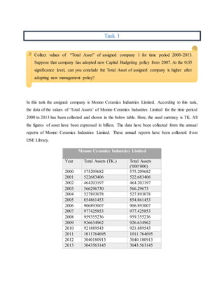
  • 1. Task 1 In this task the assigned company is Monno Ceramics Industries Limited. According to this task, the data of the values of ‘Total Assets’ of Monno Ceramics Industries Limited for the time period 2000 to 2013 has been collected and shown in the below table. Here, the used currency is TK. All the figures of asset have been expressed in billion. The data have been collected form the annual reports of Monno Ceramics Industries Limited. These annual reports have been collected from DSE Library. Monno Ceramics Industries Limited Year Total Assets (TK.) Total Assets ('000’000) 2000 575209682 575.209682 2001 522683406 522.683406 2002 464203197 464.203197 2003 566296730 566.29673 2004 527893078 527.893078 2005 854861453 854.861453 2006 906893007 906.893007 2007 977425853 977.425853 2008 959355236 959.355236 2009 926634962 926.634962 2010 921889543 921.889543 2011 1011764695 1011.764695 2012 3040180913 3040.180913 2013 3043563145 3043.563145 Collect values of “Total Asset” of assigned company 1 for time period 2000-2013. Suppose that company has adopted new Capital Budgeting policy from 2007. At the 0.05 significance level, can you conclude the Total Asset of assigned company is higher after adopting new management policy?
  • 2. The given information is that the company has taken a capital budgeting policy from 2007. So, the collected values of total assets can be divided into two sample. One is before capital budgeting policy (Before Capex) and another is after capital budgeting policy (After Capex). So, divided two samples are given below: Before Capex Year Total Assets (TK '000'000) After Capex Total Assets (TK. '000'000) 2000 575.209682 2007 977.425853 2001 522.683406 2008 959.355236 2002 464.203197 2009 926.634962 2003 566.29673 2010 921.889543 2004 527.893078 2011 1011.764695 2005 854.861453 2012 3040.180913 2006 906.893007 2013 3043.563145 In this task, two samples of information about total assets have been given. Both samples shows the amounts of total assets of different years of Monno Ceramics Industries Limited. Though both samples are of same item of same company, the samples are dependent not independent. Besides, in this case, the population is the amount of total assets of all the financial years from the inception of the company. Here, the population is defined. But, the population mean and standard deviation is not given in this task or there is no direction to collect all the population and calculate the population mean and standard deviation of population. As population mean and standard deviation is unknown, the t test is required here. Z test will not applicable here. Now, there is two types of T test for two sample test. One is for two independent variables (unpaired t test ) and other type of t test for two sample is for dependent variable ( paired t test). In this task paired t test is used. Now, step by step test of hypothesis for the collected sample is described below:
  • 3. Step 1: State 𝑯 𝟎 and 𝑯 𝟏: In this case, the null hypothesis and alternative hypothesis have to be defined. Here, the null hypothesis is that the total assets after adopting the capital budgeting policy is not higher than before taking the capital budgeting policy. On the other hand, the alternative hypothesis is that the total assets after adopting the capital budgeting policy is higher than before taking the capital budgeting policy. So, according to the alternative hypothesis, the population mean difference of the values of total assets before project and after project is more than zero. On the other hand, it is zero or less according to null hypothesis. So, expressing the two hypothesis in term we get- Step 2: Select the level of significance: The significance level is the probability that we reject the null hypothesis when it is actually true. The likelihood is determined prior to selecting the sample or performing any calculation. The 0.05 and 0.01 significance levels are the most common, but other values such as 0.02 and 0.10 can be used. In this task the level of significance has been given and it is 0.05. Step 3: Determine the test statistic: In this case, we will use t as test statistic because the population mean and population standard deviation is unknown here. But, the sample are taken form same population so, the samples are dependent. So, the t statistic will be used for two dependent sample which is also called paired t test. Step 4: Formulate a decision rule: Recall that the alternative hypothesis from Step 1 states a direction, so, this is a one tailed t test. To determine the critical value we need the level of significance which is 0.05 and degree of freedom. Now, degree of freedom for t test is n -1 . Here, n = 7. So, degree of freedom is 6. So, the critical value from the below table of t distributions is 1.943. 𝑯 𝟎: 𝝁 𝒅 ≤ 𝟎 𝑯 𝟏: 𝝁 𝒅 > 𝟎
  • 4. So, the decision rule is that reject the null hypothesis if the calculated value of the t is more than 1.943. The null hypothesis will not be rejected if the calculated value of t is equal or less than 1.943.
  • 5. Step 5: Make decision and interpret the result: In this task we have to calculate the value of t using smallstata 12 software and interpret the result. To do this task we have to follow some steps. So step by step process of finding the value of t is given below: t value calculation using Smallstata 12 Firstly, the small smallstat 12 program have to be opened and br (browse ) command have to be given to get new data editor file which is given in the below graph: Now, edit mode of the data file have to be activated and enter the values total assets before capital budgeting policy in the first column and after capital budgeting policy in the second column. Then we have to save the data file. The screenshot of data file is given below: Decision making and interpretation using STATA
  • 6. Now, we have to open the saved data file for task 1 and give the br command to browse the file. Then we have to give the command of paired t test to find the value of t. Here, the software command will be- Giving the above mentioned command and pressing enter we will find the following result page: Stata Command for Paired t test: ttest After_Capex = Before_Capex
  • 7. Interpretation of the result found using STATA Interpretation of the result of the found using smallstata 12 is the most crucial part of this task. The screenshot of the output box is given below with proper interpretation of the result:
  • 8. Here, there are two variables. One is total assets after capital budgeting policy and another is total assets before capital budgeting policy. Here, the calculated value of t using stata is 2.8851 which is more than the critical value of 1.943. So, according to the decision rule, the null hypothesis is rejected. Because, the calculated value of t falls in the rejection area. So, as the null hypothesis is rejected, the alternative hypothesis is accepted. So the interpretation of the rejecting null hypothesis is like the following sentence. We can conclude that the value of the population mean of the total assets of Monno Ceramics Industries Limited more than as before. This means that, the taking of new capital budgeting policy will increase the total assets of the company. P- Value based decision: The P value based decision rule is to reject the null hypothesis if the p value is smaller than level of significance. If p value is larger than level of significance then null hypothesis is not rejected. Here, the alternative hypothesis is that the Ha: (mean diff) > 0. So, here the value of p is 0.0139 which is smaller than level of significance of 0.05. So, the null hypothesis is rejected here. We can conclude that the value of the population mean of the total assets of Monno Ceramics Industries Limited more than as before. This means that, the taking of new capital budgeting policy will increase the total assets of the company. We can also find the value of t using MS Excel. Here, we have to use the data analysis tool pack in excel. Here, we have to select the ‘t -Test : Paired Two Sample for Means’ to find the value of t, the critical value of t and p vale for this t test for paired variables. After selecting the tool and adequate data range and output range. We will find the following output using the data we have collected for this task. Decision making and interpretation using MS Excel
  • 9. Here, the calculated value of t using Data Analysis Tool Pack of MS Excel is 2.885071681 which is more than the critical value of 1.94180281. So, according to the decision rule, the null hypothesis is rejected. Because, the calculated value of t falls in the rejection area. So, as the null hypothesis is rejected, the alternative hypothesis is accepted. So the interpretation of the rejecting null hypothesis is like the following sentence. We can conclude that the value of the population mean of the total assets of Monno Ceramics Industries Limited more than as before. This means that, the taking of new capital budgeting policy will increase the total assets of the company. P- Value based decision: The P value based decision rule is to reject the null hypothesis if the p value is smaller than level of significance. If p value is larger than level of significance then null hypothesis is not rejected. Here the value of p is 0.013936189 which is smaller than level of significance of 0.05. So, the null hypothesis is rejected here. We can conclude that the value of the population mean of the total assets of Monno Ceramics Industries Limited more than as before. This means that, the taking of new capital budgeting policy will increase the total assets of the company. t-Test: Paired Two Sample for Means After_Capex Before_Capex Mean 1554.40205 631.1486504 Variance 1033456.788 30619.08582 Observations 7 7 Pearson Correlation 0.9759851 Hypothesized Mean Difference 0 df 6 t Stat 2.885071681 P(T<=t) one-tail 0.013936198 t Critical one-tail 1.943180281 P(T<=t) two-tail 0.027872396 t Critical two-tail 2.446911851
  • 10. In this step, the value of t will be calculated. For, paired t test, the formula for t statistic is given below: 𝑡 = 𝑑̅ 𝑆 𝑑 √ 𝑛⁄ Now, the detail calculation of t statistic is shown below. Here the difference of total assets of two samples have to be calculated first and then the mean difference and standard deviation of difference have to be computed to use this in t statistic calculation. Before Capex Year Total Assets (TK. '000'000) After Capex Total Assets (TK '000'000) Differences (𝒅) 𝒅 − 𝒅̅ (𝒅− 𝒅̅) 𝟐 2000 575.209682 2007 977.425853 402.216171 -521.0372281 271479.7931 2001 522.683406 2008 959.355236 436.67183 -486.5815691 236761.6234 2002 464.203197 2009 926.634962 462.431765 -460.8216341 212356.5785 2003 566.29673 2010 921.889543 355.592813 -567.6605861 322238.5411 2004 527.893078 2011 1011.764695 483.871617 -439.3817821 193056.3505 2005 854.861453 2012 3040.180913 2185.31946 1262.066061 1592810.742 2006 906.893007 2013 3043.563145 2136.670138 1213.416739 1472380.182 Here, n = 7 ∑ 𝒅 = 6462.773794 0 ∑(𝒅 − 𝒅̅) 𝟐 = 4301083.811 Now, the mean difference is: 𝑑̅ = ∑ 𝑑 𝑛 = 𝟔𝟒𝟔𝟐. 𝟕𝟕𝟑𝟕𝟗𝟒 7 = 𝑇𝐾. 923.2533991 𝑏𝑖𝑙𝑙𝑖𝑜𝑛 Now, the standard deviation of differences is : Decision making and interpretation of the result (Manually)
  • 11. 𝑆 𝑑 = √ ∑(𝒅 − 𝒅̅) 𝟐 𝑛 − 1 = √ 𝟒𝟑𝟎𝟏𝟎𝟖𝟑. 𝟖𝟏𝟏 7 − 1 = 𝑇𝐾. 846.6683541 𝑏𝑖𝑙𝑙𝑖𝑜𝑛 Now using the previous mentioned formula of t statistic, the calculated value of t is as follows: 𝑡 = 𝑑̅ 𝑆 𝑑 √ 𝑛⁄ = 923.2533991 846.6683541 √7⁄ = 2.885071681 Now , the calculated value of t which is 2.885 is more than the critical value of 1.943. So, according to the decision rule the null hypothesis is rejected. Because, the calculated value of t falls in the rejection area. So, as the null hypothesis is rejected , the alternative hypothesis is accepted. So the interpretation of the rejecting null hypothesis is like the following sentence. We can conclude that the value of the population mean of the total assets of Monno Ceramics Industries Limited more than as before. This means that, the taking of new capital budgeting policy will increase the total assets of the company. P value based decision: The P value based decision rule is to reject the null hypothesis if the p value is smaller than level of significance. If p value is larger than level of significance then null hypothesis is not rejected. Here, level of significance is 0.05 and degree of freedom is 6 and it is one tailed t test. Besides, the calculated value of t is 2.89. The finding the value of p as follows:
  • 12. So, here, we have to the row of 6 degree of freedom and we have to search for 2.89. We have found two values one is 2.447 and another is 3.143. So, our calculated t is between these two values. Now for one tailed test the level of significance for this two values are 0.025 and 0.01. So, the value of p will be a value between 0.025 and 0.01. The exact value of p can be calculated using statistical software like stat, SPPSS etc. Now the value of p is smaller than the level of significance which is 0.05, so according to decision rule null hypothesis is rejected. We can conclude that the value of the population mean of the total assets of Monno Ceramics Industries Limited more than as before. This means that, the taking of new capital budgeting policy will increase the total assets of the company.
  • 13. Task 2 In this task, for group 20, the assigned company 1 is Monno Ceramics Industries Limited. The second assigned company is Jamuna Oil Company Limited and the third company which has chosen by the members of group 20 is Agricultural Manufacturing Company Limited (PRAN). According to this task, the information of the ‘Inventory’ figure from the balance sheet of these companies from 2009 to 2013 have been collected and summarized in the below graph. This information of inventory figures have been collected from the annual report of these companies. These annual reports have been collected form the BSE Library: Treatment 1 (MCIL) TK. Treatment 2 (JOCL) TK. Treatment 3 (AMCL- PRAN) TK. 319582782 4680130510 481449835 328571701 5763969084 491757780 342480370 5732912051 514774187 281849243 7846806129 534462767 297663954 8326552026 549659858 Now, in order to make the calculation and interpretation more clear, these information of inventory figures have to converted into billion (TK. ‘000’000). So, the converted format will be as follows: Treatment 1 (MCIL) TK(‘000’000) Treatment 2 (JOCL) TK(‘000’000) Treatment 3 (AMCL- PRAN) TK(‘000’000) 319.582782 4680.13051 481.449835 328.571701 5763.969084 491.75778 342.48037 5732.912051 514.774187 281.849243 7846.806129 534.462767 297.663954 8326.552026 549.659858
  • 14. Now, the five step test of hypothesis procedure will be used to test the hypothesis about the population statistics. Step 1: State the null hypothesis and the alternative hypothesis: Here, the null hypothesis is that the mean amount of inventories for all three companies are same. 𝑯 𝟎: 𝝁 𝟏 = 𝝁 𝟐 = 𝝁 𝟑 The alternative hypothesis is that the mean inventories are not all the same for the three airlines. 𝑯 𝟏: 𝑻𝒉𝒆 𝒎𝒆𝒂𝒏 𝒊𝒏𝒗𝒆𝒏𝒕𝒐𝒓𝒊𝒆𝒔 𝒂𝒓𝒆 𝒏𝒐𝒕 𝒂𝒍𝒍 𝒆𝒒𝒖𝒂𝒍 We can also think of alternative hypothesis as “at least two mean inventories are not equal.” If the null hypothesis is not rejected, we can conclude that there is no difference in mean inventories of all three companies. If null hypothesis is rejected, we conclude that there is a difference in at least one pair of mean inventories, but at this point we do not know which pair or how many pairs differ. Step 2: Select the level of significance: In this task the level of significance has been given and it is 0.05. Step 3: Determine the test statistic: Here, test statistic follows F distribution. ANOVA test have to be performed here. The test of ANOVA is used to compare the population mean of more than two population. Step 4: Formulate decision rule: To determine decision rule we need critical value. In order to find out critical value, the degree of freedom and level of significance are needed to know first. Here, the level of significance is 0.05 and now we have to know the degree of freedom for numerator and denominator. The degree of freedom for numerator equals the number of treatments, designated as k minus 1. On the other hand, the degree of numerator is the total number of observations, n, minus the number of treatments. For this task there are 3 treatments and 15 observations.
  • 15. The degree of freedom in the numerator = k -1 = 3 -1 = 2 The degree of freedom in the denominator = n – k = 15 – 3 = 12 Now we will look at the following table of F distributions to find out the critical value. Move horizontally across the top of the table to 2 degree of freedom in the numerator. Then move down that column to the row with 12 degree of freedom. The value at this intersection is 3.89. So, the decision rule is to reject 𝑯 𝟎 if the computed value of F exceeds 3.89.
  • 16. Step 5: Make decision and interpret the result: In this task, the ANOVA table have to be derived using smallstata software to find out the value of F statistic. Besides, we have to interpret the result. So, the step is divided into two part. One is derivation of ANOVA table and second is the interpretation of the result found using STATA. Construction of ANOVA Table using STATA: Firstly, the small smallstat 12 program have to be opened and br (browse ) command have to be given to get new data editor file which is given in the below graph: Here, we have 3 treatments of one variable which is inventory. So, we have to conduct one way F test. So, we have to construct in a different way. At first column, the name of the company have to be shown. At first to show the values of inventory from 2009 to 2013 of Monno Ceramics Industry Limited, we have type “Monno” in five consecutive rows of the first column and show the value in the respective rows of the right column which is showing the values of inventory. In Decision making and interpretation using STATA
  • 17. the same way , the value of Jamuna Oli Company Limited and AMCL – PRAN have to entered into the data file to use in stata. So the constructed data file in stata will be as follows: Now, we have to open the saved data file for task 2 and give the br command to browse the file. Then we have to give the command of F statistic or ANOVA test to find the value of F. The ANOVA test in this case is one way. So, it’s command is very simple. We have to type “oneway”. Then we have to give a space ,then we have to mention the variable ‘Invenotry’ which has been created in data file. After giving another space we have to mention the variable ‘Company’ which is used here to show three treatments. Here, the software command will be- Stata Command for One way ANOVA Test: oneway Inventory Company
  • 18. Giving the above mentioned command and pressing enter we will find the following result page: Interpretation of the result found using STATA Interpretation of the result of the found using smallstata 12 is the most crucial part of this task. The screenshot of the output box is given below with proper interpretation of the result:
  • 19. Here, the ANOVA table has been derived using the one way ANOVA test command using STATA. Here, the sum squares of sources of variation between groups is Tk. 122344737 billion. The sum squared within the groups is Tk. 9593391.07 billion. Here, degree of freedom for numerator is 2 and degree of freedom for denominator is 12. So, the critical value here is 3.89. Now the software result of F is 76.52 which is fur more than critical value. So, the null hypothesis is rejected. We conclude that the population mean are not all equal that means the population mean of Inventory of figure of all the financial years of three companies are not identical or equal. So, there is a variation in mean figure of “Invnetory” among Monno Ceramics Industries Limited, Jamuna Oil Company Limited, and AMCL –PRAN. But, we cannot specify exact which company differ and by how much amount. P –value based decision: The P value based decision rule is to reject the null hypothesis if the p value is smaller than level of significance. If p value is larger than level of significance then null hypothesis is not rejected. The value of p found from the stata solution is about 0.000 which is smaller than the level of significance of 0.05. So, the null hypothesis is rejected. We conclude that the population mean are not all equal that means the population mean of Inventory of figure of all the financial years of three companies are not identical or equal. We can also derive ANOVA table and value of F using data analysis tool pack in excel. For this task we have to use single factor ANOVA test, because we have used one variable and it is ‘Inventory’. After mentioning the input ranges in excel and using anova: single factor toll , the following result will be shown in the mentioned output range or output ply page. Decision making and interpretation using MS Excel
  • 20. Here, we have used 3 treatments which are three assigned company. Here, the critical value or table value is 3.885294 and the value of F is 76.51813811 which is greater than the critical value. So, the null hypothesis is rejected. We conclude that the population mean are not all equal that means the population mean of Inventory of figure of all the financial years of three companies are not identical or equal. So, there is a variation in mean figure of “Invnetory” among Monno Ceramics Industries Limited, Jamuna Oil Company Limited, and AMCL –PRAN. But, we cannot specify exact which company differ and by how much amount. P –value based decision: The P value based decision rule is to reject the null hypothesis if the p value is smaller than level of significance. If p value is larger than level of significance then null hypothesis is not rejected. The value of p found using the data analysis tool pack is about 0.000 which is smaller than the level of significance of 0.05 which is given in this task. So, the null hypothesis is rejected. We conclude that the population mean are not all equal that means the population mean of Inventory of figure of all the financial years of three companies are not identical or equal. Anova: Single Factor SUMMARY Groups Count Sum Average Variance Monno Ceramics Ltd. 5 1570.14805 314.02961 588.7916478 Jamuna Oil Ltd. 5 32350.3698 6470.07396 2396947.901 AMCL- PRAN 5 2572.10443 514.4208854 811.0733852 ANOVA Source of Variation SS df MS F P-value F crit Between Groups 122344737 2 61172368.54 76.51813811 0.00 3.885294 Within Groups 9593391.07 12 799449.2554 Total 131938128 14
  • 21. It is convenient to summarize the calculations of the F statistic in an ANOVA table. The format for an ANOVA table is as follows. Statistical software packages also use this format. ANOVA Table Source of Variation Sum of Squares Degree of Freedom Mean Square F Treatments SST k -1 SST/(k -1) =MST MST / MSE Error SSE n -1 SSE / (n – k) = MSE Total SS Total n -1 There are three values or sum of squares, used to compute the test statistic F. These values can be determined by obtaining SS total and SSE., then finding SST by subtraction. The SS total term is the total variation, SST is the variation due to the treatments, and SSE is the variation within the treatments or the random error. The process can be started by finding SS total. This is the sum of the squared differences between each observation and the overall mean. The formula for finding SS total is: 𝑆𝑆 𝑡𝑜𝑡𝑎𝑙 = ∑(𝑋 − 𝑋 𝐺 ̅̅̅̅)2 Where, X is each sample observation. 𝑋 𝐺 ̅̅̅̅ is the overall or grand mean. Next determine SSE or the sum of the squared errors. This is the sum of the squared differences between each observation and its respective treatment mean. The formula for finding SSE is: 𝑆𝑆𝐸 = ∑(𝑋 − 𝑋 𝑐 ̅̅̅)2 Where, 𝑋 𝑐 ̅̅̅ is the sample mean for treatment C. Decision making and interpretation of the result (Manually)
  • 22. So, the detailed calculation of SS total and SSE for this task is given below: Calculation of SS total: Now, to find out the SS total we have to find out the grand mean first. Here, there are 15 observations and the total is Tk. 36492.62228 billion. So, the grand mean is TK. 2432.841485 billion. 𝑋 𝐺 ̅̅̅̅ = 36492.62228 15 = 2432.841485 MCIL TK.('000'000) JOCL TK.('000'000) AMCL- PRAN TK. ('000'000) Total TK. ('000'000) 319.582782 4680.13051 481.449835 328.571701 5763.969084 491.75778 342.48037 5732.912051 514.774187 281.849243 7846.806129 534.462767 297.663954 8326.552026 549.659858 Column total 1570.14805 32350.3698 2572.104427 36492.62228 n 5 5 5 15 Mean 314.02961 6470.07396 514.4208854 2432.841485 Next we find the deviation of each observation from the grand mean, square those deviations, and sum this result for all 15 observations. This work finding differences is summarized in the below table: MCIL TK.('000'000) JOCL TK.('000'000) AMCL- PRAN TK. ('000'000) -2113.2587 2247.289025 -1951.39165 -2104.26978 3331.127599 -1941.083705 -2090.36112 3300.070566 -1918.067298 -2150.99224 5413.964644 -1898.378718
  • 23. -2135.17753 5893.710541 -1883.181627 Now, square each of these differences and sum all the values to find our SS total is shown in the below table: MCIL TK.('000'000) JOCL TK.('000'000) AMCL- PRAN TK. ('000'000) SS Total 4465862.346 5,050,308 3807929.372 4427951.324 11,096,411 3767805.95 4369609.592 10,890,466 3678982.16 4626767.626 29,311,013 3603841.757 4558983.089 34,735,824 3546373.041 Total 22449173.98 91,084,022 18404932.28 131938128.1 Calculation of SSE: To compute the term SSE find the deviation between each observation and its treatment mean. In computation differences of each observation with its respective mean is shown in the below table: MCIL TK.('000'000) JOCL TK.('000'000) AMCL- PRAN TK. ('000'000) 5.553172 -1789.94345 -32.9710504 14.542091 -706.104876 -22.6631054 28.45076 -737.161909 0.3533016 -32.180367 1376.732169 20.0418816 -16.365656 1856.478066 35.2389726 Each of these values is squared and then summed for all 15 observations. The values are shown in the following table: MCIL TK.('000'000) JOCL TK.('000'000) AMCL- PRAN TK. ('000'000) SSE TK. ('000'000)
  • 24. 30.83771926 3203897.554 1087.090164 211.4724107 498584.0959 513.6163464 809.4457446 543407.6801 0.124822021 1035.57602 1895391.465 401.6770181 267.8346963 3446510.81 1241.78519 Total 2355.166591 9587791.605 3244.293541 9593391.065 So the SSE value is TK. 9593391.065 billion. Finally, we have to determine SST which is SST minus SSE. 𝑆𝑆𝑇 = 𝑆𝑆 𝑡𝑜𝑡𝑎𝑙 − 𝑆𝑆𝐸 𝑆𝑆𝑇 = 131938128.1− 9593391.065 = 122344737.1 Construction of ANOVA Table: To find the computed value of F, the ANOVA table have to be constructed. The degree of freedom for the numerator and denominator are the same as in step 4. The term mean square is another expression for an estimate of the variance. The mean square for treatments is SST divided by its degree of freedom. The result is the mean square for treatments and is written MST. Computation of the mean square error is in the same fashion. To be precise, divide SSE by its degree of freedom to find MSE. .To complete the process and find the value of F , we have to divide MST by MSE. So, summarized ANOVA table to find F using MS Excel is given below: ANOVA Table Source of Variation Sum of Squares Degree of Freedom Mean Square F Treatments 122344737.1 2 61172368.54 76.51813811 Error 9593391.065 12 799449.2554 Total SS Total 14 Now, the computed value of F is 76.51813811 which is greater than the critical value of 3.89, so the null hypothesis is rejected. We conclude that the population mean are not all equal that means
  • 25. the population mean of Inventory of figure of all the financial years of three companies are not identical or equal. So, there is a variation in mean figure of “Invnetory” among Monno Ceramics Industries Limited, Jamuna Oil Company Limited, and AMCL –PRAN. But , we cannot specify exact which company differ and by how much amount.