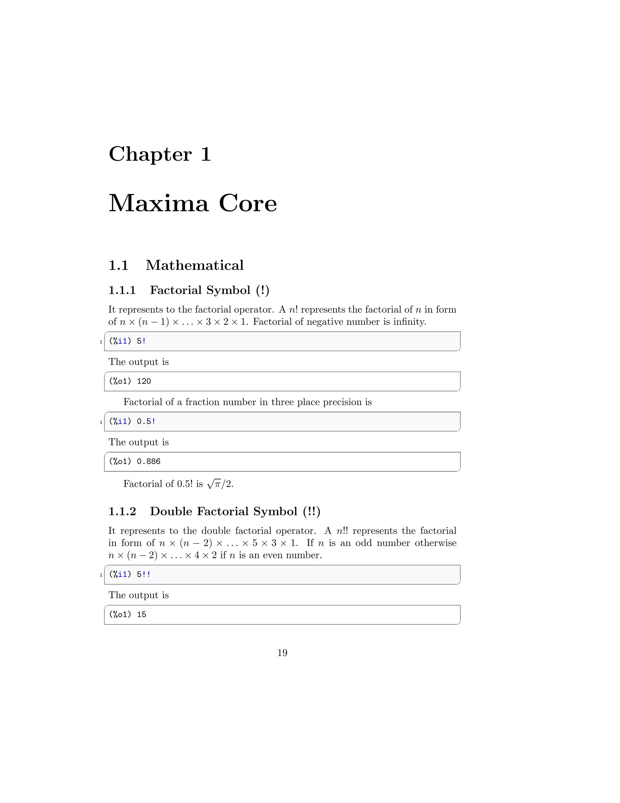
This document provides an overview of commands and functions in the Maxima computer algebra system. It includes sections on mathematical commands, errors, procedural commands, and declarations. Some key commands and functions discussed include factorial (!), variable assignment (:), function definition (:=), arithmetic operators (+ - * /), comparison operators (< > <= >=), and procedural commands like quit, read, and time. The document serves as a reference for the core functionality available in the Maxima system.


![Contents
I Modelica Commands 17
1 Maxima Core 19
1.1 Mathematical . . . . . . . . . . . . . . . . . . . . . . . . . . . . . 19
1.1.1 Factorial Symbol (!) . . . . . . . . . . . . . . . . . . . . . 19
1.1.2 Double Factorial Symbol (!!) . . . . . . . . . . . . . . . . 19
1.1.3 Termination of Line (;) . . . . . . . . . . . . . . . . . . . 20
1.1.4 Negation of Expression (#) . . . . . . . . . . . . . . . . . 20
1.1.5 Evaluate Internally & No Output ($) . . . . . . . . . . . . 20
1.1.6 Do Not Execute Function (’) . . . . . . . . . . . . . . . . 20
1.1.7 Re-evaluation of Specific Input (“) . . . . . . . . . . . . . 21
1.1.8 Variable Assigning Operator (:) . . . . . . . . . . . . . . . 21
1.1.9 Operator Assigner (::) . . . . . . . . . . . . . . . . . . . . 21
1.1.10 Macro Function Definition Operator (::=) . . . . . . . . . 22
1.1.11 Function Operator (:=) . . . . . . . . . . . . . . . . . . . 22
1.1.12 Sum Operator (+) . . . . . . . . . . . . . . . . . . . . . . 23
1.1.13 Subtraction Operator (-) . . . . . . . . . . . . . . . . . . . 23
1.1.14 Product Operator (*) . . . . . . . . . . . . . . . . . . . . 24
1.1.15 Division Operator (/) . . . . . . . . . . . . . . . . . . . . 24
1.1.16 Exponential Operator (ˆ) . . . . . . . . . . . . . . . . . . 25
1.1.17 Equal Operator (=) . . . . . . . . . . . . . . . . . . . . . 26
1.1.18 Less Than Operator (<) . . . . . . . . . . . . . . . . . . . 26
1.1.19 Grater Than Operator (>) . . . . . . . . . . . . . . . . . 26
1.1.20 Less Than or Equals To Operator (<=) . . . . . . . . . . 27
1.1.21 Greater Than or Equals To Operator (>=) . . . . . . . . 27
1.1.22 Lisp Name (?) . . . . . . . . . . . . . . . . . . . . . . . . 27
1.1.23 A List ([ ... ]) . . . . . . . . . . . . . . . . . . . . . . . . . 27
1.1.24 Call Last Garbage (%) . . . . . . . . . . . . . . . . . . . . 28
1.1.25 Previous Statement (%%) . . . . . . . . . . . . . . . . . . 28
1.1.26 Exponential (%e) . . . . . . . . . . . . . . . . . . . . . . . 28
1.1.27 %e to numlog . . . . . . . . . . . . . . . . . . . . . . . . . 29
1.1.28 Negative Exponent as a Quotient (%edispflag) . . . . . . 29
1.1.29 Demoivre Mode (%emode) . . . . . . . . . . . . . . . . . 29
1.1.30 Exponential Numerical (%enumer) . . . . . . . . . . . . . 29
1.1.31 Gamma Constant (%gamma) . . . . . . . . . . . . . . . . 30
3](https://image.slidesharecdn.com/maximacasanintroduction-211010145450/75/Maxima-CAS-an-introduction-3-2048.jpg)

![20 CHAPTER 1. MAXIMA CORE
1.1.3 Termination of Line (;)
Symbol ‘;’ (colon) is used to terminate a line in Maxima console. Every thing
written after the symbol ‘;’ is treated as comments and it is skipped by Maxima
during evaluation of transcript.
✞
1 (%i1) 5!!; double factorial
✆
The output is
✞
(%o1) 15
✆
1.1.4 Negation of Expression (#)
# represents negation of syntactic equality. Note that because of the rules for
evaluation of predicate expressions “not a = b” is equivalent tois(a # b) instead
of “a # b”.
1.1.5 Evaluate Internally & No Output ($)
$ restrict the evaluation of expression internally and the result is not printed in
output console. This operator is always post fixed to transcripts. The syntax is
✞
1 (%i1) <transcript> $
✆
For example
✞
1 (%i1) matrix([1,2],[3,4])$
✆
will be evaluated internally and there is no output in console. Remember that
this symbol must not followed by any string or digits or comments.
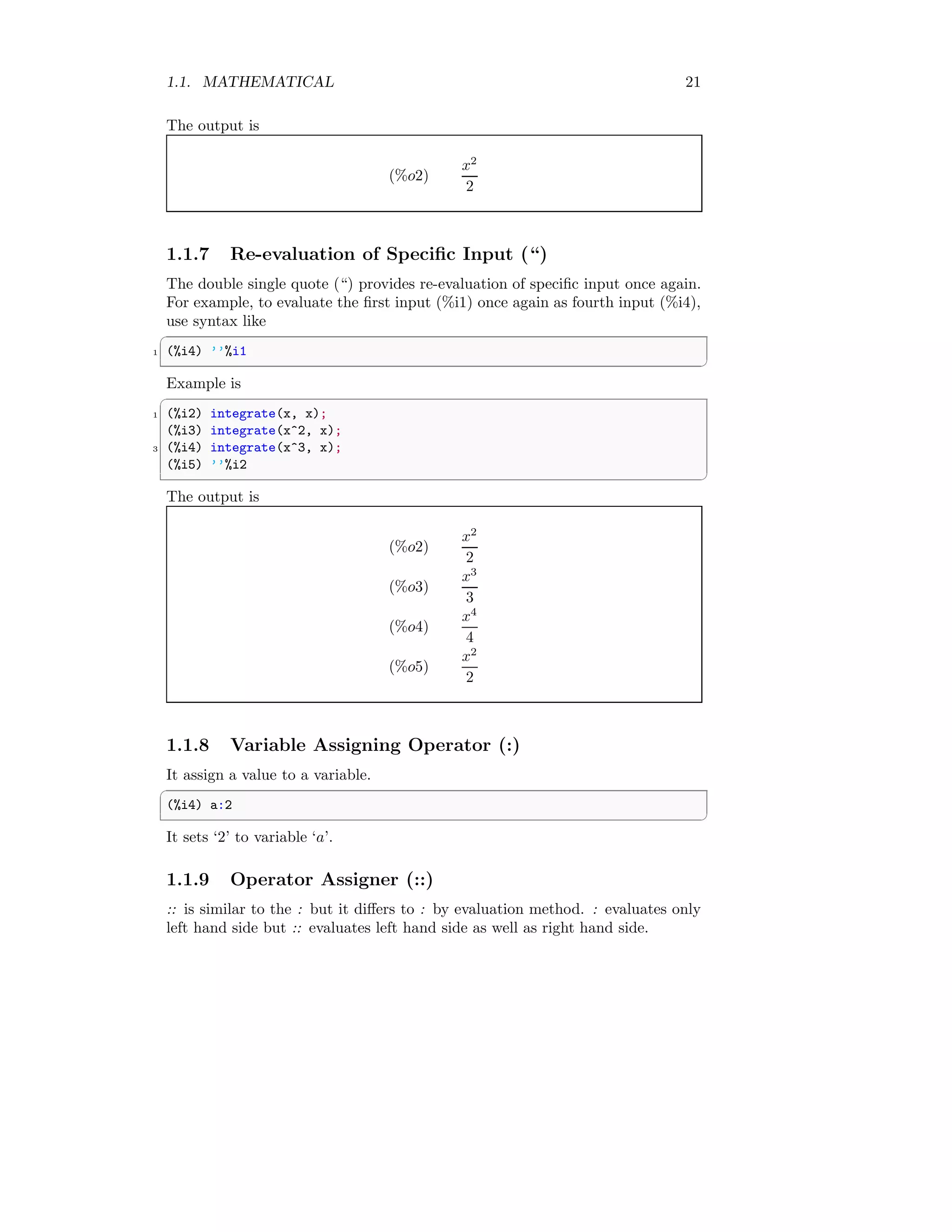
1.1.6 Do Not Execute Function (’)
If a function is prefixed with (’) then function is not executed. It just returns
the argument.
✞
1 (%i1) ’integrate(x,x)
✆
The output is
(%o1)
Z
x dx
and function without prefix with (’)
✞
1 (%i2) integrate(x,x)
✆](https://image.slidesharecdn.com/maximacasanintroduction-211010145450/75/Maxima-CAS-an-introduction-20-2048.jpg)
![22 CHAPTER 1. MAXIMA CORE
✞
1 (%i4) y:[a,b,c];%initializing operators
(%i5) y::[10,11,12];%initializing values
3 (%i6) a;%call operator ’a’
✆
✞
(%o4) 10
✆
1.1.10 Macro Function Definition Operator (::=)
::= defines a function which quotes its arguments, and the expression which it
returns is evaluated in the context from which the macro was called.
✞
1 (%i4) g(x) ::= x/99;
(%i5) g(9999);
✆
✞
(%o5) 101
✆
1.1.11 Function Operator (:=)
:= is used to initialize a function. := never evaluates the function body. The
syntax for function operator is like
✞
1 (%i4) <function name>(<independent variable>):=<function body>
✆
For example
✞
1 (%i4) f(x):=sin(x)
✆
(%o4) f(x) := sin(x)
To call the function use following syntax.
✞
1 (%i4) f(<independent variable value>)
✆
If user defined function body consists in-build functions then result is just sym-
bolic otherwise it gives numeric result. For example
✞
1 (%i4) f(x):=sin(x);
(%i5) f(10);
✆
(%o5) sin(10)
To get the numerical result rather than symbolic result then the syntax becomes
like](https://image.slidesharecdn.com/maximacasanintroduction-211010145450/75/Maxima-CAS-an-introduction-22-2048.jpg)
![1.1. MATHEMATICAL 27
1.1.20 Less Than or Equals To Operator (<=)
It is mathematical operator that tells whether the left hand side is lesser than
or equals to the right hand side term.
✞
1 (%i4) is(a <= b);
✆
✞
(%o4) unknown
✆
If terms are purely number then answer is either “true’ or ‘false’.
✞
1 (%i4) is(1 <= 2);
✆
✞
(%o4) true
✆
1.1.21 Greater Than or Equals To Operator (>=)
It is mathematical operator that tells whether the left hand side is greater than
or equals to the right hand side term.
✞
1 (%i4) is(a >= b);
✆
✞
(%o4) unknown
✆
If terms are purely number then answer is either “true’ or ‘false’.
✞
1 (%i4) is(1 >= 2);
✆
✞
(%o4) false
✆
1.1.22 Lisp Name (?)
The function name which is prefixed by ‘?’ signifies that the name is a Lisp
name, not a Maxima name.
1.1.23 A List ([ ... ])
[ ... ] represents the beginning and end of a list or vector.
✞
1 (%i4) y:[a,b,c];%initializing operators as a list
(%i5) y::[10,11,12];%initializing values as a list
3 (%i6) a;%call operator ’a’ from operator list
✆
✞
(%o4) 10
✆](https://image.slidesharecdn.com/maximacasanintroduction-211010145450/75/Maxima-CAS-an-introduction-27-2048.jpg)
![28 CHAPTER 1. MAXIMA CORE
1.1.24 Call Last Garbage (%)
Symbolic computation, tends to create a good deal of garbage (temporary or
intermediate results that are eventually not used), and effective handling of it
can be crucial to successful completion of some programs. Symbol % is used for
calling last garbage.
✞
1 (%i1) x^2+2$
(%i2) x^2-2$
3 (%i3) solve(%); % calling last garbage
✆
(%o3) [x = −
√
2 x =
√
2]
If % is suffixed by garbage handle like ‘i1’, ‘i2’ or ‘o1’, ‘o2’ etc then specific
garbage can be called.
✞
1 (%i1) x^2+2$
(%i2) x^2-2$
3 (%i3) solve(%i1); % calling first garbage
✆
(%o3) [x = −
√
2i, x =
√
2i]
1.1.25 Previous Statement (%%)
In compound statements, namely block, lambda, or (s1, ..., sn), %% is the value
of the previous statement.
1.1.26 Exponential (%e)
It represents to the exponential base. The series expansion of ‘%e’ is
ex
= 1 +
x
1!
+
x2
2!
+
x3
3!
+ . . .
If x = 1 then above series becomes
e = 1 +
1
1!
+
1
2!
+
1
3!
+ . . .
The numerical value of ‘%e’ lies between 2 < %e < 3 and actually it is ap-
proximately equals to ‘2.718281828459045’. Remember whenever you need to
substitute ‘%e’ with its numerical value, set ‘%enumer’ to true by using the
following syntax
✞
1 (%i1) %enumer:true;
✆](https://image.slidesharecdn.com/maximacasanintroduction-211010145450/75/Maxima-CAS-an-introduction-28-2048.jpg)
![1.2. ERRORS 31
accept the input as key-value like arguments rather than execute it and show
output. The key-value syntax may be in form of ‘key=value’ or ‘key:value’. If
disp executed successfully, “done” is returns as output by Maxima.
✞
1 (%i1) b[1,2]:x-x^2$
(%i2) x:123$
3 (%i3) disp(x, b[1,2], sin(1.0));
✆
✞
123
x-x^2
0.8414709848078965
(%o3) done
✆
1.2 Errors
1.2.1 Error (error)
The variable error is set to a list describing the error. The first element of error
is a format string, which merges all the strings among the arguments supplied
to error function and the remaining elements are the values of any non-string
arguments. Syntax for error function is
✞
(%i1) error(expr_1, ..., expr_n)
✆
1.2.2 Error Size (error size)
error size modifies error messages according to the size of expressions which
appear in them. If the size of an expression (as determined by the Lisp func-
tion ERROR-SIZE) is greater than error size, the expression is replaced in the
message by a symbol, and the symbol is assigned the expression. The symbols
are taken from the list error syms. The default value of error size is ‘10’.
1.2.3 Error Symbol (error syms)
In error messages, expressions larger than error size are replaced by symbols,
and the symbols are set to the expressions. The symbols are taken from the
list error syms. The first too-large expression is replaced by error syms[1], the
second by error syms[2], and so on.
1.2.4 Error Message (errormsg)
Reprints the most recent error message. The variable error holds the message,
and errormsg formats and prints it.](https://image.slidesharecdn.com/maximacasanintroduction-211010145450/75/Maxima-CAS-an-introduction-31-2048.jpg)
![1.3. PROCEDURAL 33
✞
(%i1) numer:true;
2 (%i2) %e
✆
✞
(%o2) 2.718281828459045
✆
If numer is set to ‘false’ then result is symbolic.
✞
1 (%i1) numer:false;
(%i2) %e
✆
✞
(%o2) %e
✆
1.3 Procedural
1.3.1 Interrupt Maxima (kill)
It removes all bindings (value, function, array, or rule) from the arguments. An
argument may be a symbol or a single array element. The syntax is
✞
1 (%i1) kill(symbol)
(%i2) kill([array element 1, array element 2, ...)
3 (%i3) kill(labels)
(%i4) kill(integers)
5 (%i5) kill(all)%kills all values, function, array or rules
✆
1.3.2 Modes of Variables (mode declare)
mode declare is used to declare the modes of variables and functions for subse-
quent translation or compilation of functions. mode declare is typically placed
at the beginning of definition of a function, at the beginning of a Maxima script,
or executed at the interactive prompt. The syntax used is
✞
1 (%i1) mode_declare ([y_1, y_2, ...], fixnum)%Or
✆
or
✞
1 (%i2) mode_declare (y_1, mode_1, ... y_n, mode_n])
✆
The ‘fixnum’ are “float”, “bignum” etc. For example,
✞
1 (%i1) F(x):=(mode_declare([x], float), x+2.0)
✆
This converts independent variable x as floating value and as well as function
F(x) = x + 2.0 into floating function.](https://image.slidesharecdn.com/maximacasanintroduction-211010145450/75/Maxima-CAS-an-introduction-33-2048.jpg)
![1.3. PROCEDURAL 35
1.3.8 Print the Reset Option (optionset)
When optionset is ‘true’, Maxima print outs a message whenever a Maxima
option is reset. This is useful if the user is doubtful of the spelling of some
option and wants to make sure that the variable he assigned a value to was
truly an option variable. The default value is ‘false’.
1.3.9 Play Previous Garbage (playback)
It prints the previously collected garbage by the Maxima. The syntax is
✞
1 (%i1) playback ([inputs, outputs], grind, time, slow)
✆
Argument “slow” is useful in conjunction with save or stringout when creating a
secondary-storage file in order to pick out useful expressions. Argument “time”
displays the computation time for each expression. Argument “grind” displays
input expressions in the same format as the “grind”. Output expressions are
not affected by the “grind” option.
1.3.10 Prompting Symbol (prompt)
prompt is the prompt symbol of the demo function, playback (slow) mode and
the Maxima break loop. The default value is ‘ ’.
1.3.11 Quit the Session (quit)
quit terminates the current Maxima session. It is used like quit().
1.3.12 Rationalized Print (ratprint)
When ratprint is true, a message informing the user about the conversion of
floating point numbers into rational numbers is displayed. The default value is
‘true’.
1.3.13 Enter into Lisp System (to lisp)
to lisp variable let to enter into Lisp system of Maxima. It enables to initiated
new variable, function etc in Maxima that can be used later in Maxima after
returning to Maxima. To return to Maxima,
✞
1 (%i1) to_maxima;
✆
variable is used (including parenthesis brackets).](https://image.slidesharecdn.com/maximacasanintroduction-211010145450/75/Maxima-CAS-an-introduction-35-2048.jpg)
![1.3. PROCEDURAL 37
✞
1 (%i1) integrate(x,x)
(%i2) time(%o1);
✆
✞
(%o2) [0.0]
✆
1.3.21 Promp Read (read)
read first prints the statement and then ask for one input in the console. The
expression entered in the console is read by Maxima and returns the evaluated
result of the expression in the console. The expression entered into the console
muste be terminated by dollar sign(‘$’).
✞
1 (%i1) a=10;
(%i2) f:read(Enter new value)$
3 Enter new value 2^a$
(%i3) f;
✆
✞
(%o3) 1024
✆
1.3.22 testsuite files
Similar to the run testsuite to check the test pass of a file.
✞
1 (%i1) testsuite_files();
✆
1.3.23 Test The Maxim (run testsuite)
run testsuite tests producing the desired answer are considered “passes” as are
tests that do not produce the desired answer, but are marked as known bugs.
✞
1 (%i1) run_testsuite();
✆
1.3.24 Read Function Without Evaluation (readonly)
If readonlyfunction is used in place of readfunction with similar syntax, then it
returns the expression to console without evaluation.
✞
1 (%i1) a=10;
(%i2) f:readonly(Enter new value)$
3 Enter new value 2^a$
(%i3) f;
✆
(](https://image.slidesharecdn.com/maximacasanintroduction-211010145450/75/Maxima-CAS-an-introduction-37-2048.jpg)

![1.3. PROCEDURAL 39
and Maxima returns ‘true’ then ‘expression’ is atomic (i.e. a number, name or
string) otherwise ‘expression’ is non atomic. Thus
✞
1 (%i1) atom(5)
✆
is true while
✞
1 (%i1) atom(a[1])
✆
and
✞
1 (%i2) atom(sin(x))
✆
are ‘false’ (assuming a[1] and x are unbound).
1.3.32 Declare a Function Antisymmetric (antisymmet-
ric)
Function declare, if used as the syntax given below, tells Maxima to recognize
a function as an antisymmetric function. The syntax for this flag is
✞
1 (%i1) declare(f, antisymmetric)
✆
Here function ‘f’ will assumed as an antisymmetric function.
1.3.33 Check The Integer Type (askinteger)
✞
1 (%i1) askinteger(expression, integer type)
✆
attempts to determine from the assume database whether expression is an in-
teger or not. There are three categories of ‘integer type’ - (i) “odd”, (ii) “even”
and (iii) “integer”.
1.3.34 Retrive User Property (get)
✞
1 (%i1) get(a, i)
✆
It retrieves the user property indicated by i associated with atom a or returns
‘false’ if a doesn’t have property i.
1.3.35 Declare Variable as Integer (integer)
Function declare, if used as the syntax given below, tells Maxima to recognize
a variable as an integer. The syntax for this flag is
✞
1 (%i1) declare(var, integer)
✆
Here variable ‘var’ will assumed as an integer.](https://image.slidesharecdn.com/maximacasanintroduction-211010145450/75/Maxima-CAS-an-introduction-39-2048.jpg)
![1.3. PROCEDURAL 41
1.3.40 Declare Variable as Positive (assume pos)
When assume pos is ‘true’ and the sign of a parameter x cannot be determined
from the current context or other considerations, sign and asksign (x) return
‘true’. By default it is ‘false’.
1.3.41 Declare As Communative Function (commutative)
Function declare, if used as the syntax given below, tells the simplifier that
function is a commutative function. The syntax for this is
✞
1 (%i1) declare(f, commutative)
✆
1.3.42 Compare Expression (compare)
It returns the comparative result according to the comparative relation between
two supplied arguments to the function compare. Syntax for this function is
✞
1 (%i1) compare(expr 1, expr 2)
✆
If Maxima is unable to compare then it returns “unknown”.
1.3.43 Context (context)
context names the collection of facts maintained by assume, forget. Binding con-
text to a name ‘foo’ changes the current context to ‘foo’. If the specified context
‘foo’ does not yet exist, it is created automatically by a call to newcontext. The
specified context is activated automatically. By default it is “initial”.
1.3.44 Contexts (contexts)
contexts is a list of the contexts which currently exist, including the currently
active context. By default its value is [“initial”, “global”].
1.3.45 Deactivate Context (deactivate)
deactivate deactivates the contexts supplied to the function as its arguments.
✞
1 (%i1) deactivate(context 1, context 2, .....)
✆
1.3.46 Delcaration Statement (declare)
It assigns the atom or list of atoms the property or list of properties respectively.
It is used like
✞
1 (%i1) declare(atom, property)
✆](https://image.slidesharecdn.com/maximacasanintroduction-211010145450/75/Maxima-CAS-an-introduction-41-2048.jpg)


![Chapter 5
Algebra
This section includes the functions can be used in algebra.
5.1 Linear Equations
5.1.1 Algebraic Evaluation (algebraic)
By default algebraic is ‘false’. It must be set ‘true’ in order to simplify the
algebraic numbers.
5.1.2 Solving Linear Equation (solve)
A linear equation can be solved by using solve function. An algebraic equation,
f(x) = 0 of a variable x, would be arranged in form of f(x) = 0 before getting
the roots of the equation. If equation is in form of f(x) = a then it should be
arranged as f(x) − a = 0 before supplying it as argument to the solve function.
The synopsis of the solve function is
✞
1 (%i1) solve([linear algebraic equation],[variable])
✆
Example is
✞
1 (%i1) solve([x^2-x+1=0],[x])
✆
The output is
(%o1)
x = −
√
3 i − 1
2
, x =
√
3 i + 1
2
#
If we have to solve more than one function then syntax for solve becomes
✞
1 (%i11) x+y=1
✆
63](https://image.slidesharecdn.com/maximacasanintroduction-211010145450/75/Maxima-CAS-an-introduction-63-2048.jpg)
![64 CHAPTER 5. ALGEBRA
(%o11) x + y = 1
✞
1 (%i12) x-y=2
✆
(%o12) x − y = 2
✞
1 (%i13) solve([%o11,%o12])
✆
(%o12)
y = −
1
2
, x =
3
2
5.1.3 Simplify Logs, Exponent Radicals (radcan)
radcan simplifies expressions, which contain logs, exponentials and radicals. For
a somewhat larger class of expressions, radcan produces a regular form. Two
equivalent expressions in this class do not necessarily have the same appearance,
but their difference can be simplified by radcan to zero. For example
log(x + x2
) − log(x)
a
[log(1 + x)]
a/2
= [log(x + 1)]
a/2
Maxima code is
✞
1 (%i3) radcan((log(x+x^2)-log(x))^a/log(1+x)^(a/2));
✆
(%o3) log (x + 1)
a
2
5.1.4 Radical Expansion (radexpand)
By default it is ‘true’. It controls the expansion of radicals. When it is ‘true’
for all, factors are pulled outside to the radicals. For example, when radexpand
is ‘true’,
√
4x2 becomes 2x as a coefficient of the expression.
5.1.5 Rational Simplification (ratsimp)
It is abbrevation of “rational simplification”. It simplifies the expression and all
of its subexpressions, including the arguments to non-rational functions. The](https://image.slidesharecdn.com/maximacasanintroduction-211010145450/75/Maxima-CAS-an-introduction-64-2048.jpg)
![5.2. INEQUALITY POLYNOMIAL 67
✞
(%i3) equal(x, x^2);
2 (%i4) is(%);
✆
(%o4) unknown
✞
(%i3) equal(x*x,x^2);
2 (%i4) is(%);
✆
(%o4) true
5.2.2 Inequality (notequal)
notequal compares two expressions, whether two expressions are equal or not.
The stat of comparison is returned when it is asked by using function is. It is
used for false state.
✞
(%i3) notqual(x, x^2);
2 (%i4) is(%);
✆
(%o4) unknown
✞
(%i3) notequal(x*x,x^2);
2 (%i4) is(%);
✆
(%o4) false
5.2.3 Solve Algebraic Polynomials (algsys)
algsys used to solve the simultaneous polynomial equations for the list of the
variables. All the polynomial equations and list of variables to be supplied as
arguments to the function must be in vector form. The syntax used is
✞
(%i3) algsys([s^3+1], [s]);
✆](https://image.slidesharecdn.com/maximacasanintroduction-211010145450/75/Maxima-CAS-an-introduction-67-2048.jpg)
![68 CHAPTER 5. ALGEBRA
(%o3)
s = −1
s =
√
3 i + 1
2
s = −
√
3 i − 1
2
5.2.4 Solve Linear Equations (linsolve)
linsolve is used to solve the simultaneous linear equations for the list of variables.
The expressions must be polynomials in the variables and may be equations.
All the linear equations and list of variables to be supplied as arguments to the
function must be in vector form. The syntax used is
✞
1 (%i3) linsolve([2*x+8*y-4*z=10, 2*x+y+4*z=8, x-8*y-z=-20], [x, y, z]);
✆
(%o3) x = −
45
89
y =
198
89
z =
151
89
5.2.5 Check The Stat Of Database (is)
is attempts to determine whether the predicate expression is provable from the
facts in the assume database. If the proven state from the facts is not assumed
then it returns the status ‘unknown’.
✞
1 (%i3) notequal(x*x, x^2);
(%i4) is(%);
✆
(%o4) false
5.2.6 Check The Stat Of Database (maybe)
maybe similar to is, attempts to determine whether the predicate expression
is provable from the facts in the assume database. If state is not assumed in
database, it returns ‘unknown’ result.
✞
(%i3) notequal(x, x^2);
2 (%i4) maybe(%);
✆](https://image.slidesharecdn.com/maximacasanintroduction-211010145450/75/Maxima-CAS-an-introduction-68-2048.jpg)


![7.2. DERIVATIVE 75
✞
1 (%i5) diff(
function,
3 var 1,
order var 1,
5 var 2,
order var 2, ...
7 )
✆
Example is
✞
1 (%i5) ’diff(sin(x)*cos(y),x,2,y,2);
✆
(%o5)
d4
dx2 dy2
[sin(x) cos(y)]
If ‘independent variable’ is not provided then the result contains
✞
1 del(independent variable)
✆
that represents to the differential of ‘independent variable’ and return value is
so called “total differential”. For example
y = cos(x) × sin(x)
Its total derivative is
dy = cos2
(x) − sin2
(x)
dx
Single variable example in Maxima is
✞
1 (%i5) diff(sin(x)*cos(x))
✆
(%o5) (cos2
(x) − sin2
(x)) del(x)
A multivariable example is
✞
1 (%i5) diff(sin(x)*cos(y))
✆
(%o5) cos(x) cos(y) del(x) − sin(x) sin(y) del(y)
diff function can be used with integrate function to evaluate relation for “deriva-
tive of integral” written as
d
dx
Z b(x)
a(x)
f(t) dt
Maxima example is given like](https://image.slidesharecdn.com/maximacasanintroduction-211010145450/75/Maxima-CAS-an-introduction-75-2048.jpg)
![76 CHAPTER 7. CALCULUS
✞
1 (%i5) diff(
integrate(
3 cos(t),
t,
5 0,
x^2
7 ),
x,
9 1
);
✆
(%o5) 2x cos(x2
)
7.2.2 Partial Drivative (gradef)
7.2.3 Total Differential (del)
If ‘independent variable’ is not provided then the result contains del(¡independent
variable¿) that represents to the differential of ‘independent variable’ and return
value is so called “total differential”. Single variable example is
✞
(%i5) diff(sin(x)*cos(x))
✆
(%o5) (cos2
(x) − sin2
(x)) del(x)
A multivariable example is
✞
1 (%i5) diff(sin(x)*cos(y))
✆
(%o5) cos(x) cos(y) del(x) − sin(x) sin(y) del(y)
A functional defferentiation can be obtained by using function diff like the
syntax.
✞
1 (%i5) depends([f,g],u);
(%i5) diff(f*g,u);
✆
(%o5) f
d
d u
g
+
d
d u
f
g](https://image.slidesharecdn.com/maximacasanintroduction-211010145450/75/Maxima-CAS-an-introduction-76-2048.jpg)
![7.2. DERIVATIVE 77
7.2.4 Dependence of Function (depends)
Suppose f and g are two independent functions and they are dependend of
u then the function will be like f(u) and g(u). Here functions f and g are
dependent to variable u. To define the dependency of function to independent
variable, depends function is used like the syntax
✞
(%i5) depends(function, dependent variable)
✆
Functions may be dependent to one or more variables. The syntax will be
modified like
✞
1 (%i5) depends(
[function 1,function 2],
3 [dependent var 1, dependent var 2]
)
✆
Here functions and independent variables are in vector form. A combination
of vector and scalar for functions and independent variables can also be used.
Single function and single variable xample is
✞
(%i5) depends (f, x);
✆
(%o5) [f(x)]
Multi-functions and multi-variables example is
✞
1 (%i5) depends ([r, s], [u, v, w]);
✆
(%o5) [r(u, v, w), s(u, v, w)]
7.2.5 Show Dependencies (dependencies)
It returns the previously defined dependent functions. The syntax used is
✞
1 (%i5) dependencies;
✆
7.2.6 Notation of Derivative (derivabbrev)
When derivabbrev is ‘true’, symbolic derivatives are displayed as subscripts.
Otherwise, derivatives are displayed in the Leibniz notation dy/dx.
✞
1 (%i4) derivabbrev:true;
(%i5) diff(f(x),x)
✆](https://image.slidesharecdn.com/maximacasanintroduction-211010145450/75/Maxima-CAS-an-introduction-77-2048.jpg)
![78 CHAPTER 7. CALCULUS
(%o5) f(x)x
7.2.7 Value of Function at a Point (atvalue)
atvalue assigned a value to function when condition is met. The syntax used is
✞
(%i5) atvalue(function, conditions, rep value)
✆
This function is used to assign boundary values to a function. For example,
when x = 0 and y = 0 then assign function f(x, y) value ‘a’. The syntax is
✞
1 (%i5) atvalue(f(x,y), [x=0,y=0], a)
✆
(%o5) a
If ‘rep value’ is not a constant value and it is expression consisting independent
variables ‘x’ and ‘y’ then first independent variable of function is represented
as ‘@1’ and second indpenedent variable is represented as ‘@2’ and so on. For
example
✞
1 (%i5) atvalue(f(x,y), [x=0,y=0], x+y)% first var = x second var =y
✆
(%o5) @2 + @1
Example of three variables function with two variables condition and replace-
ment value.
✞
1 (%i5) atvalue(f(x,z,y), [x=0,y=0], x+y) % first var = x third var =y
✆
(%o5) @3 + @1
7.2.8 Degree of Derivative (derivdegree)
Returns the highest degree of derivative of dependent variable y with respect to
the independent variable x occuring in expression. The syntax used is
✞
1 (%i5) atvalue(expression, dependent var, independent var)
✆
Here ‘expression’ may be a function name or a differential equation.](https://image.slidesharecdn.com/maximacasanintroduction-211010145450/75/Maxima-CAS-an-introduction-78-2048.jpg)

![84 CHAPTER 8. ORDINARY DIFFERENTIAL EQUATION
✞
1 (%i5) bc2(y=x+%k1+%k2, x=0, y=1, x=1, y=2);
✆
(%o5) y = x + 1
8.1.2 Linear Ordinary Differential Equations (desolve)
The function desolve solves systems of linear ordinary differential equations
using Laplace transform. The syntax used is
✞
1 (%i5) desolve ([eqn_1, ..., eqn_n], [x_1, ..., x_n])
✆
For example
✞
1 (%i5)
✆
(%o5)
8.1.3 Initial Value Problem of First Order (ic1)
A first-order ordinary differential equation is either in form of
dy
dx
= F(x, y)
or in form of
dy
dx
+ p(x) y = q(x)
and its solution is
y =
R h
e
R
p(x) dx
i
q(x) dx + c
e
R
p(x) dx
To get the constant value ‘c’, we substitute the initial values in the solution of
first order differential equation. The value of ‘c’ is again put into the solution
of first order equation and finally it gives the final solution. The function ic1
solves initial value problem of first order differential equation. It accepts three
arguments. ‘solution’ is the solution of first order differential equation. It has
one constant whose value is obtained by substituting initial boundary values
(x1, y1). The syntax used is
✞
1 (%i5) ic1 (solution, x_1, y_1)
✆
For example](https://image.slidesharecdn.com/maximacasanintroduction-211010145450/75/Maxima-CAS-an-introduction-84-2048.jpg)
![8.2. ODE 85
8.1.4 Initial Value Problem of Second Order (ic2)
A second-order linear ODE with variable coefficients
d2
y
dx2
+ p(x)
dy
dx
+ q(x)y = 0
Solution of this equation is
?
The function ic2 solves initial value problem of second order differential equa-
tion. It accepts four arguments. ‘solution’ is the solution of second order differ-
ential equation. It has one constant, k, and one derivative of dependent variable
with respect to independent variable, dy/dx, after first anti-derivative of second
order differential equation. Before performing second anti-derivative to get final
solution of second order differential equation, constant k is obtained by sub-
stituting the initial boundary values and derivative value, [dy/dx]x1,y1
at the
initial boundary value in the ‘solution’. The syntax used is
✞
1 (%i5) ic2 (solution, x_1, y_1, deriv x_1 y_1)
✆
For example
8.2 ODE
8.2.1 Ordinary Deferential Equation of Second Order (ode2)
The function ode2 solves an ordinary differential equation (ODE) of first or
second order. It receives three arguments, ‘solution’, ‘dependent variable’ and
‘independent variable’. The syntax used is
✞
1 (%i5) ode2 (equation, dependent variable, independent variable)
✆
For example
✞
1 (%i5) ode2(’diff(y,x) -y = 1, y,x);
✆
(%o5) y = %c − e−x
ex](https://image.slidesharecdn.com/maximacasanintroduction-211010145450/75/Maxima-CAS-an-introduction-85-2048.jpg)

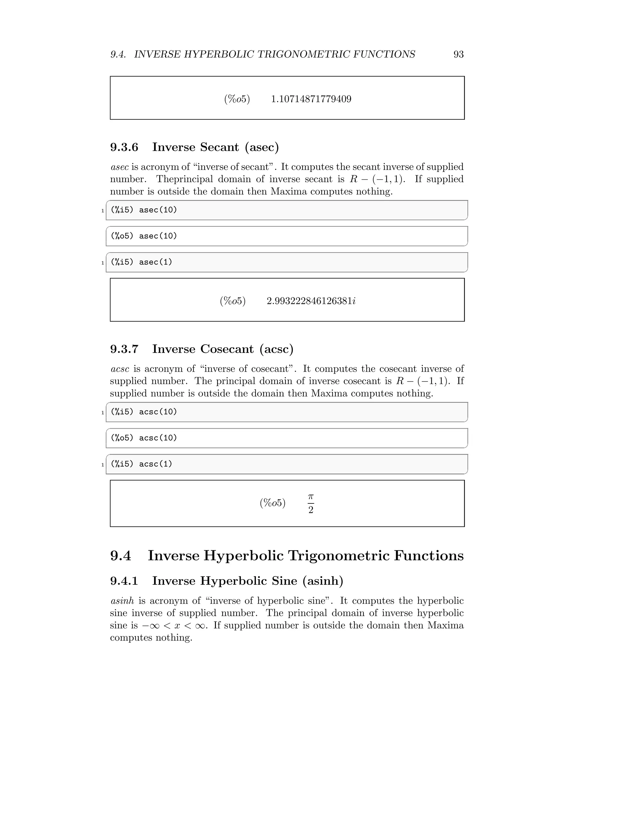
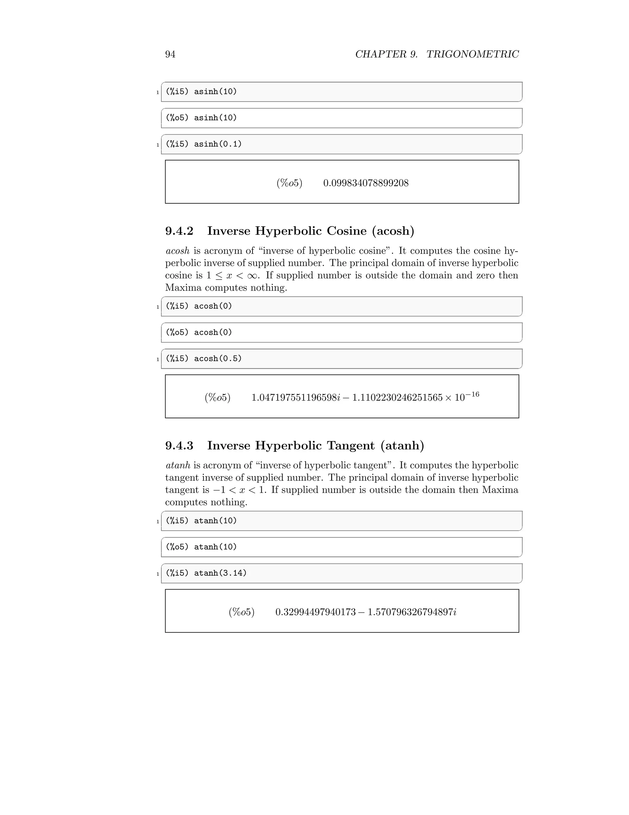
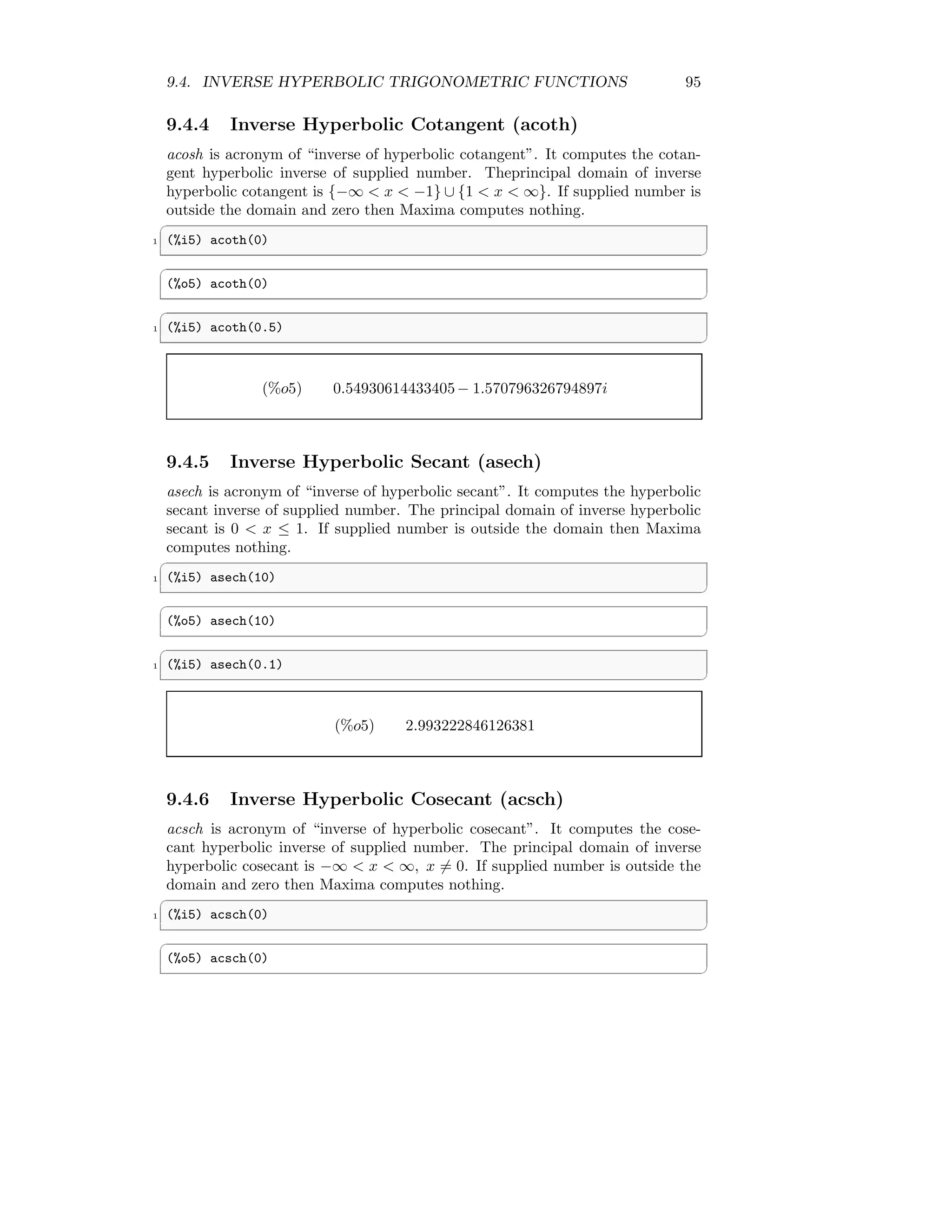
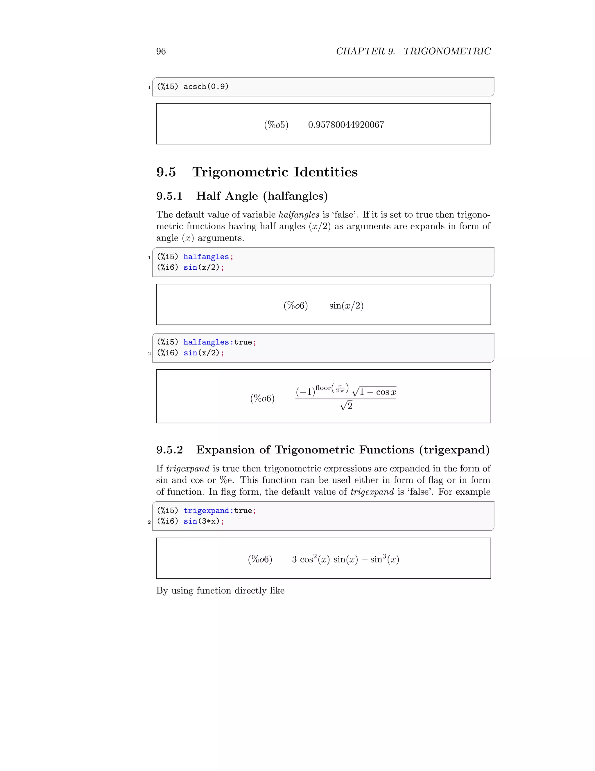
![9.3. INVERSE TRIGONOMETRIC FUNCTIONS 91
9.2.5 Hyperbolic Secant (sech)
sech is acronym of “hyperbolic secant”. It computes the hyperbolic secant of
supplied argument in radian. The principal domain of hyperbolic secant is R.
If supplied argument is outside the domain then Maxima computes nothing.
✞
1 (%i5) sech(10)
✆
✞
(%o5) sech(10)
✆
✞
1 (%i5) sech(0)
✆
(%o5) 1
9.2.6 Hyperbolic Cosecant (csch)
The principal domain of hyperbolic cosecant is R − {0}.
9.3 Inverse Trigonometric Functions
9.3.1 Inverse Sine (asin)
asin is acronym of “inverse of sine”. It computes the sine inverse of supplied
number. The principal domain of inverse sine is [−1, 1]. If supplied number is
outside the domain then Maxima computes nothing.
✞
1 (%i5) asin(10)
✆
✞
(%o5) asin(10)
✆
✞
1 (%i5) asin(1)
✆
(%o5)
π
2
9.3.2 Inverse Cosine (acos)
acos is acronym of “inverse of cosine”. It computes the cosine inverse of supplied
number. The principal domain of inverse cosine is [−1, 1]. If supplied number
is outside the domain then Maxima computes nothing.](https://image.slidesharecdn.com/maximacasanintroduction-211010145450/75/Maxima-CAS-an-introduction-91-2048.jpg)
![Chapter 10
Matrix
Following functions are useful for matrices.
10.1 Mathematical Operaton
10.1.1 Matrix (matrix)
The function matrix constructs a matrix of order m × n where m is number of
rows and n is number of columns. The syntax for function matrix is
✞
(%io) A:matrix([row 1], [row 2], ..., [row n]);
✆
For example
✞
1 (%i1) A:matrix([1,2,3],[2,1,3],[4,7,4]);
✆
(%o1)
1 2 3
2 1 3
4 7 4
10.1.2 Scalar Addition of Matrices (+)
The operator + adds two matrices element by element wise. If A = Pij and
B = Qij are two matrices then the addition of two matrices will be
Cij = A + B = Pij + Qij
In addition of two matrices corresponding elements are added together and
output is a matrix. Addition operation is performed only if two matrices are of
same order.
101](https://image.slidesharecdn.com/maximacasanintroduction-211010145450/75/Maxima-CAS-an-introduction-101-2048.jpg)
![102 CHAPTER 10. MATRIX
✞
1 (%i1) A:matrix([1,2,3],[2,1,3],[4,7,4]);
(%i2) B:matrix([1,2,3],[2,1,3],[4,7,4]);
3 (%i3) A+B;
✆
(%o3)
2 4 6
4 2 6
8 14 8
10.1.3 Scalar Subtraction of Matrices (-)
The operator - subtract two matrices element by element wise. If A = Pij and
B = Qij are two matrices then the subtraction of matrix B from A will be
Cij = A − B = Pij − Qij
In subtraction of matrix B from matrix A, corresponding elements are sub-
tracted with each other and result is a matrix. Subtraction operation is per-
formed only if two matrices are of same order.
✞
1 (%i1) A:matrix([2,2,3],[2,4,3],[4,7,4]);
(%i2) B:matrix([1,2,3],[2,1,3],[4,7,4]);
3 (%i3) A-B;
✆
(%o3)
1 0 0
0 3 0
0 0 0
10.1.4 Scalar Multiplication of Matrices (*)
The operator * multiply two matrices element by element wise. If A = Pij and
B = Qij are two matrices then the multiplication of matrix B to A will be
Cij = A ∗ B = Pij ∗ Qij
In scalar multiplication of matrix B to matrix A, corresponding elements are
multiply with each other and result is a matrix. Multiplication operation is
performed only if two matrices are of same order.
✞
1 (%i1) A:matrix([2,2,3],[2,4,3],[4,7,4]);
(%i2) B:matrix([1,2,3],[2,1,3],[4,7,4]);
3 (%i3) A*B;
✆](https://image.slidesharecdn.com/maximacasanintroduction-211010145450/75/Maxima-CAS-an-introduction-102-2048.jpg)
![10.1. MATHEMATICAL OPERATON 103
(%o3)
2 4 9
4 4 9
16 49 16
10.1.5 Scalar Division of Matrix (/)
The operator / divides two matrices element by element wise. If A = Pij and
B = Qij are two matrices then the division of matrix A by matrix B will be
Cij = A/B = Pij/Qij
In scalar division of matrix A by matrix B is performed by dividing elements of
A by corresponding elements of B. Division operation is performed only if two
matrices are of same order.
✞
1 (%i1) A:matrix([2,2,3],[2,4,3],[4,7,4]);
(%i2) B:matrix([1,2,3],[2,1,3],[4,7,4]);
3 (%i3) A/B;
✆
(%o3)
2 1 1
1 4 1
1 1 1
10.1.6 Exponent of Matrix (ˆ)
The operator ˆ raises power of element of one matrix to the base of another
matrix element by element wise. If A = Pij and B = Qij are two matrices then
the exponent AB
will be
Cij = AB
= Pij
Qij
Exponent operation is performed only if two matrices are of same order.
✞
1 (%i1) A:matrix([2,2,3],[2,4,3],[4,7,4]);
(%i2) B:matrix([1,2,3],[2,1,3],[4,7,4]);
3 (%i3) A^B;
✆
(%o3)
2 2 3
2 4 3
4 7 4
1 2 3
2 1 3
4 7 4
](https://image.slidesharecdn.com/maximacasanintroduction-211010145450/75/Maxima-CAS-an-introduction-103-2048.jpg)
![104 CHAPTER 10. MATRIX
If exponent power is not a matrix but is a number then all elements of base
matrix are raised to the power by the number.
✞
1 (%i1) A:matrix([2,2,3],[2,4,3],[4,7,4]);
(%i2) A^2;
✆
(%o3)
4 4 9
4 16 9
16 49 16
If exponent operator is ˆˆ then exponent is noncommutative matrix exponenti-
ation. A scalar base to a matrix power is carried out element by element.
10.1.7 Matrix Dot Product (.)
The dot operator,is for non-commutative multiplication of two matrices. When
“.” is preceded and followed by spaces e.g. A · B, then it distinguishes plainly
from a decimal point in a floating point number. If two vectors are ~
A = 1î +
2ĵ + 3k̂ and ~
B = 3î + 4ĵ + 5k̂ then A · B is given by
A · B = (1î + 2ĵ + 3k̂) · (3î + 4ĵ + 5k̂)
On simplification
A · B = 26
In dot product, both lists or vectors or non-commutative matrices should be of
same order. An example is
✞
(%i5) a:[1,2,3];
2 (%i6) b:[3,4,5];
(%i7) a . b;
✆
(%o7) 26
Another example
✞
1 (%i5) a:[1,2,3];
(%i6) b:[8,9];
3 (%i7) a . b;
✆
✞
(%o7) MULTIPLYMATRICES: attempt to multiply nonconformable matrices.
✆](https://image.slidesharecdn.com/maximacasanintroduction-211010145450/75/Maxima-CAS-an-introduction-104-2048.jpg)
![10.2. INVERSE OF MATRIX 105
10.2 Inverse of Matrix
10.2.1 Invert of Matrix Elements (Aˆ-1)
If exponent power is −1 over a matrix then elementwise inversion of elements
of the matrix are take place. If Aij is an element of a matrix A then A−1
is a
matrix of the elements 1/Aij.
✞
1 (%i1) A:matrix([2,2,3],[2,4,3],[4,7,4]);
(%i2) A^-1;
✆
(%o3)
1/2 1/2 1/3
1/2 1/4 1/3
1/4 1/7 1/4
10.2.2 Inverse of a Matrix (Aˆˆ-1)
Noncommutative exponential ˆˆ is followed by ‘−1’ to a matrix is matrix inver-
sion. If A is a square matrix then Aˆˆ-1 is matrix inverse.
✞
(%i1) A:matrix([2,2,3],[2,4,3],[4,7,4]);
2 (%i2) A^^-1;
✆
(%o3)
5/8 −13/8 3/4
−1/2 1/2 0
1/4 3/4 −1/2
10.2.3 Append Columns (addcol)
addcol appends one or more lists or matrix, Bp×q, in given matrix Am×n as
columns of matrix Am×n. Row size of matrix Bp×q ie p should be equal to the
row size of matrix Am×n ie m.
✞
(%i5) A:matrix([1,2,3],[4,1,2],[5,4,2]);
2 (%i6) B:matrix([2,1,3],[3,1,2],[3,4,4]);
(%i7) addcol(A,B)
✆
(%o7)
1 2 3 2 1 3
4 1 2 3 1 2
5 4 2 3 4 4
](https://image.slidesharecdn.com/maximacasanintroduction-211010145450/75/Maxima-CAS-an-introduction-105-2048.jpg)
![106 CHAPTER 10. MATRIX
10.2.4 Append Rows (addrow)
addrow appends one or more lists or matrix, Bp×q, in given matrix Am×n as
rows of matrix Am×n. Column size of matrix Bp×q ie q should be equal to the
column size of matrix Am×n ie n.
✞
1 (%i5) A:matrix([1,2,3],[4,1,2],[5,4,2]);
(%i6) B:matrix([2,1,3],[3,1,2],[3,4,4]);
3 (%i7) addrow(A,B)
✆
(%o7)
1 2 3
4 1 2
5 4 2
2 1 3
3 1 2
3 4 4
10.2.5 Ajoint of Matrix (adjoint)
adjoint returns the adjoint of a matrix A. The adjoint matrix is the transpose
of the matrix of co-factors of A. Co-factor about an element Aij is the (−1)i+j
times determinant of sub-matrix found by removing ith
row and jth
column.
For obtaining adjoint matrix, the matrix must be a square matrix.
✞
1 (%i5) A:matrix([1,2,3],[4,1,2],[5,4,2]);
(%i6) adjoint(A)
✆
(%o6)
−6 8 1
2 −13 10
11 6 −7
10.2.6 Augmented Matrix (augcoefmatrix)
augcoefmatrix returns the augmented coefficient matrix for the variables x1, x2,
. . ., xn of the system of linear equations eqn1, . . ., eqnm. This is the coeffi-
cient matrix with a column adjoined for the constant terms in each equation.
In otherwords, each equation forms one row of the matrix and its coefficients
construct columns for that row. The syntax is
✞
(%i6) augcoefmatrix(
2 equaion lists,
[first variable, second variable]
4 );
✆](https://image.slidesharecdn.com/maximacasanintroduction-211010145450/75/Maxima-CAS-an-introduction-106-2048.jpg)
![10.2. INVERSE OF MATRIX 107
✞
(%i5) A:[2*x + 3*y =4, -x + 6*y =10]$
2 (%i6) augcoefmatrix(A, [x,y]);
✆
(%o6)
2 3 −4
−1 6 −10
10.2.7 Cauchy Matrix (cauchy matrix)
cauchy matrix returns a n × m Cauchy matrix with the elements
a[i, j] = 1/(xi + yi)
The second argument of cauchy matrix is optional. In this case Cauchy matrix
with the elements
a[i, j] = 1/(xi + xi)
The syntax for Cauchy matrix is
✞
(%i6) cauchy_matrix([x_1, x_2, ..., x_m],[y_1, y_2, ..., y_n]);
✆
or
✞
1 (%i6) cauchy_matrix([x_1, x_2, ..., x_n]);
✆
For example, With two input arguments for Cauchy matrix
✞
1 (%i5) cauchy_matrix([a,b],[c,d])
✆
(%o5)
1
c + a
1
d + a
1
c + b
1
d + b
A single argument Cauchy matrix
✞
1 (%i5) cauchy_matrix([a,b])
✆
(%o5)
1
2 a
1
b + a
1
b + a
1
2 b
](https://image.slidesharecdn.com/maximacasanintroduction-211010145450/75/Maxima-CAS-an-introduction-107-2048.jpg)
![108 CHAPTER 10. MATRIX
10.2.8 Characteristics Polynomial (charpoly)
charpoly returns the characteristic polynomial of the matrix A with respect to
variable x. The characteristics polynomial of a matrix A is given by
|A − λI|
The Maxima syntax equivalent to charpoly is
✞
1 (%i5) determinant(A - diagmatrix(length(A), x))
✆
✞
1 (%i5) matrix([1,2],[3,4])$
(%i6) charpoly(%,x);
✆
✞
(%o5) (1-x)(4-x)-6
✆
10.2.9 Coefficient Matrix (coefmatrix)
coefmatrix returns the coefficient matrix for the variables x1, x2, . . ., xm of the
system of linear equations eqn1, . . ., eqnm. In otherwords, each equation forms
one row of the matrix and its coefficients construct columns for that row. The
syntax is
✞
1 (%i6) coefmatrix(
equaion lists,
3 [first variable, second variable]
);
✆
✞
(%i5) A:[2*x + 3*y =4, -x + 6*y =10]$
2 (%i6) coefmatrix(A, [x,y]);
✆
(%o6)
2 3
−1 6
It differs to the augcoefmatrix as it ignores the linear equation equality value.
10.2.10 Columns of Matrix (col)
col returns the ith
column from a matrix A. The value of i must be less than
or equal to the size of column of the matrix A. The return value is a matrix.
The syntax for the function col is
✞
(%i1) col(matrix, column number);
✆](https://image.slidesharecdn.com/maximacasanintroduction-211010145450/75/Maxima-CAS-an-introduction-108-2048.jpg)
![10.2. INVERSE OF MATRIX 109
10.2.11 Column Vectors (columnvector)
It returns the column vector of size provided as argument to the function colum-
nvector. The syntax used is
✞
1 (%i1) columnvector(number of rows);
✆
Another function covect can also be used for the same purpose.
10.2.12 Copy Matrix (copymatrix)
It returns a copy of the matrix A. This is the only way to make a copy aside
from copying A element by element. The syntax used is
✞
1 (%i1) copymatrix(matrix name);
✆
10.2.13 Determinant Of Matrix (determinant)
determinant computes the determinant value of a matrix A. Symbolically it is
represented by |A|.
✞
1 (%i1) A:matrix([2,1,1],[1,2,4],[1,3,4]);
(%i2) determinant(A);
✆
✞
(%o2) -7
✆
10.2.14 Determinant As Fraction (detout)
By default the variable detout is ‘false’. When detout is ‘true’, the determinant
of a matrix whose inverse is computed is factored out of the inverse. For this
switch to have an effect of doallmxops and doscmxops and these switches should
be set to ‘false’.
✞
1 (%i5) A:matrix([1,2,3],[4,1,2],[5,4,2])$
(%i6) detout: true$
3 (%i7) doallmxops: false$
(%i8) doscmxops: false$
5 (%i6) invert(A);
✆
(%o7)
−6 8 1
2 −13 10
11 6 −7
31](https://image.slidesharecdn.com/maximacasanintroduction-211010145450/75/Maxima-CAS-an-introduction-109-2048.jpg)
![110 CHAPTER 10. MATRIX
10.2.15 Diagonal Matrix (diagmatrix)
It returns a diagonal matrix of size n × n with the diagonal elements all equal
to x. The syntax is
✞
1 (%i1) diagmatrix(square matrix size, diagonal variable x)
✆
For example
✞
1 (%i5) diagmatrix(3,a)
✆
(%o5)
a 0 0
0 a 0
0 0 a
10.2.16 Do All Matrix Operations (doallmxops)
When doallmxops is ‘true’, all operations relating to matrices are carried out.
When it is ‘false’ then the setting of the individual dot switches govern which
operations are performed. By default doallmxops is ‘true’.
10.2.17 Do Exponent Operations (domxexpt)
When domxexpt is ‘true’, a matrix exponential, exp(A) where A is a matrix, is
interpreted as a matrix with element [i, j] equals to exp (M[i, j]). Otherwise
exp(A) evaluates to exp (ev(A)). domxexpt affects all expressions of the form
basepower
where ‘base’ is an expression assumed scalar or constant, and ‘power’
is a list or matrix.
10.2.18 Do Matrix-Matrix Operations (domxmxops)
When domxmxops is ‘true’, all matrix-matrix or matrix-list operations are car-
ried out (but not scalar-matrix operations); if this switch is ‘false’ such opera-
tions are not carried out. By default it is “false’.
10.2.19 Do Matrix Products (domxnctimes)
When domxnctimes is ‘true’, non-commutative products of matrices are carried
out. By default it is “false’.
10.2.20 Do Not Factorize (dontfactor)
dontfactor may be set to a list of variables with respect to which factoring is
not to occur.](https://image.slidesharecdn.com/maximacasanintroduction-211010145450/75/Maxima-CAS-an-introduction-110-2048.jpg)
![112 CHAPTER 10. MATRIX
10.2.30 Zero Exponsnt (dotident)
Default value of dotident is ‘1’. dotident is the value returned by Xˆˆ0.
10.2.31 Dot Screw Rules (dotscrules)
By default dotscrules is ‘false’. When dotscrules is true, an expression A · C or
C · A simplifies to C ∗ A and A · (C ∗ B) simplifies to C ∗ (A · B).
10.3 Matrix Characteristics
10.3.1 Echelon Form of Matrix (echelon)
echelon computes and returns the echelon form of a matrix by using Gaussian
row elimination method. The echelon form is computed from matrix A by
elementary row operations such that the first non-zero element in each row in
the resulting matrix is one and the column elements under the first one in each
row are all zero. The matrix used in this function is of the form of m × n. The
syntax used is
✞
1 (%i2) echelon(matrix name);
✆
For example
✞
1 (%i1) A:matrix([2,0,0],[2,2,4],[2,2,4])$
(%i2) echelon(A);
✆
(%o2)
1 0 0
0 1 2
0 0 0
10.3.2 Eigenvalues (eivals)
The eigenvalue equation for a matrix A is
Av − λv = 0
which is equivalent to
(A − λI)v = 0
where I is the n×n identity matrix. All possible values of λ are called eigenvalues
of the given matrix. The function eivals evaluates the eigenvalues of the given
matrix. This function returns two list of values. The first sublist of the return
value is the list of eigenvalues of the matrix, and the second sublist is the list of
the multiplicities of the eigenvalues in the corresponding order.](https://image.slidesharecdn.com/maximacasanintroduction-211010145450/75/Maxima-CAS-an-introduction-112-2048.jpg)
![10.3. MATRIX CHARACTERISTICS 113
✞
(%i1) A:matrix([2,0,0],[2,2,4],[2,2,4]);
2 (%i2) eivals(A);
✆
✞
(%o2) [[0,2,6], [1,1,1]]
✆
10.3.3 Eigenvectors (eivects)
Computes eigenvectors of the matrix A. The return value is a list of two ele-
ments. The first is a list of the eigenvalues of A and a list of the multiplicities
of the eigenvalues. The second is a list of lists of eigenvectors. There is one list
of eigenvectors for each eigenvalue. There may be one or more eigenvectors in
each list.
✞
1 (%i1) A:matrix([2,0,0],[2,2,4],[2,2,4])$
(%i2) eivals(A)$
3 (%i3) eivects(A);
✆
✞
(%o2) [[0,1,-1/2],[1,-1/2,-1/2],[0,1,1]]
✆
10.3.4 Except Matrix (ematrix)
The syntax used in ematrix is
✞
1 (%i1) ematrix(rows, cols, value, row pos, col pos)
✆
It constructs a matrix A whose all values are zero except that Aij = x. Where
x, i and j represents to the ‘value’, ‘row pos’ and ‘col pos’ respectively. For
example
✞
1 (%i1) ematrix(3,3,a,2,2)
✆
(%o1)
0 0 0
0 a 0
0 0 0
10.3.5 User Matrix (entermatrix)
entermatrix returns a matrix of size m × n by accepting elements from the user
interactively. The syntax is
✞
1 (%i1) entermatrix(rows, cols)
✆
After pressing enter key, total elements equals to m × n are asked to enter by
user in the console and laterly a matrix is returned using these entered elements.
This function is useful to create a matrix of own choice.](https://image.slidesharecdn.com/maximacasanintroduction-211010145450/75/Maxima-CAS-an-introduction-113-2048.jpg)
![114 CHAPTER 10. MATRIX
10.3.6 Generate Matrix (genmatrix)
genmatrix generates a matrix of given size by using a function. The syntax of
function genmatrix is
✞
1 (%i2) genmatrix(gen function, rows, cols)
✆
For example
✞
1 (%i1) h[i,j]:=i+j$
(%i2) genmatrix(h,3,3)
✆
(%o2)
2 3 4
3 4 5
4 5 6
10.3.7 Identity Matrix (ident)
ident stands for identity matrix. It generates a square matrix of size n whose
other than diagonal elements are zero. Syntax for ident is
✞
(%i1} ident(square matrix size)
✆
10.3.8 Inverse Matrix (invert)
invert returns the inverse matrix of square matrix A. If A is normal square
matrix then inverse matrix is A−1
and relation between normal square matrix
and inverse matrix is A · A−1
= I. A matrix is invertible if |A| 6= 0 or constant
terms in its characteristics polynomial is not zero.
✞
1 (%i5) A:matrix([1,2,3],[4,1,2],[5,4,2])$
(%i6) invert(A)
✆
(%o6)
−
6
31
8
31
1
31
2
31
−
13
31
10
31
11
31
6
31
−
7
31
](https://image.slidesharecdn.com/maximacasanintroduction-211010145450/75/Maxima-CAS-an-introduction-114-2048.jpg)
![10.3. MATRIX CHARACTERISTICS 115
10.3.9 List Elements of Matrix (list matrix entries)
It returns the elements of a matrix A in form of list.
✞
(%i1) A:matrix([2,0,0],[2,2,4],[2,2,4])$
2 (%i2) list_matrix_entries(A);
✆
✞
(%o2) [2, 0, 0, 2, 2, 4, 2, 2, 4]
✆
10.3.10 Left Side Delimiter (lmxchar)
This variable sets the left side delimiter of the matrix. Default value is ‘[’. New
left side matrix delimiter is set by using this variable like
✞
1 (%i1) lmxchar: | % A vertical line
✆
10.3.11 Right Side Delimiter (rmxchar)
This variable sets the right side delimiter of the matrix. Default value is ‘]’.
New right side matrix delimiter is set by using this variable like
✞
1 (%i1) rmxchar: | % A vertical line
✆
10.3.12 Adjoin Matrix (adjoin)
It returns the union of the set A with matrix or list B. adjoin complains if A
is not a literal set. adjoin and union are equivalent; however, adjoin may be
somewhat faster than union.
✞
1 (%i5) adjoin (c, {a, b});
(%i6) adjoin (a, {a, b});
✆
✞
(%o5) {a, b, c}
(%o6) {a, b}
✆
10.3.13 Transpose of a Matrix (transpose)
Transpose of a matrix is the replacement of rows with columns or vice verse. It
is represented by A′
. Determinant of matrix A and its transpose are equal.
✞
(%i5) A:matrix([1,2,3],[4,1,2],[5,4,2]);
2 (%i6) transpose(A)
✆](https://image.slidesharecdn.com/maximacasanintroduction-211010145450/75/Maxima-CAS-an-introduction-115-2048.jpg)
![116 CHAPTER 10. MATRIX
(%o6)
1 4 5
2 1 4
3 2 2
10.3.14 Mapping of Matrix (matrixmap)
10.3.15 Expression As Matrix (matrixp)
Returns ‘true’ if the expression is a matrix. Syntax for the function matrixp is
✞
(%i1) matrixp(matrix name)
✆
10.3.16 Trace of Matrix (mattrace)
mattrace returns the trace of the square matrix A. Tracing of a matrix is the
sum of all elements in main diagonal of the matrix A. To evaluate tracing of
matrix, first load the “nchrpl” macro.
✞
1 (%i4) load (nchrpl);
(%i5) A:matrix([1,2,3],[4,1,2],[5,4,2]);
3 (%i6) mattrace(A);
✆
✞
(%o6) 4
✆
10.3.17 Minor of Matrix (minor)
minor returns the Mij minor of a matrix A. The syntax used is
✞
1 (%i6) minor(matrix, row, column);
✆
Minor Mij, of a matrix A is obtained by removing ith
row and jth
column. For
example
✞
1 (%i5) A:matrix([1,2,3],[4,1,2],[5,4,2]);
(%i6) minor(A,1,1)
✆
(%o6)
1 2
4 2](https://image.slidesharecdn.com/maximacasanintroduction-211010145450/75/Maxima-CAS-an-introduction-116-2048.jpg)
![10.3. MATRIX CHARACTERISTICS 117
10.3.18 Determinant of Matrix (newdet)
newdet computes the determinant of the matrix A by the Johnson-Gentleman
tree minor algorithm. newdet returns the result in CRE form.
10.3.19 Permanent of Matrix (permanent)
permanent computes the permanent of the matrix A by the Johnson-Gentleman
tree minor algorithm. A permanent is like a determinant but with no sign
changes. permanent returns the result in CRE form.
10.3.20 Rank of Matrix (rank)
Rank of a matrix is the number of non zero rows of a matrix when it is simplified
in echelon form. Rank of matrix
A =
1 2
4 2
is ‘2’ while rank of matrix
A =
1 2 3
1 1 4
0 0 0
is also ‘2’ though matrices A and B are of different orders. The syntax for
function rank is
✞
(%i3) rank(matrix)
✆
✞
1 (%i1) A:matrix([2,2,3],[2,4,3],[4,7,4]);
(%i2) rank(A);
✆
✞
(%o2) 3
✆
10.3.21 Rationalize to Matrix (ratmx)
When ratmx is ‘false’, determinant and matrix addition, subtraction, and mul-
tiplication are performed in the representation of the matrix elements and cause
the result of matrix inversion to be left in general representation.
10.3.22 Row of Matrix (row)
row returns the jth
row from a matrix A. The value of j must be less than or
equal to the size of row of the matrix A. The return value is a matrix. The
syntax for the function row is
✞
1 (%i1) row(matrix, row number);
✆](https://image.slidesharecdn.com/maximacasanintroduction-211010145450/75/Maxima-CAS-an-introduction-117-2048.jpg)
![118 CHAPTER 10. MATRIX
10.3.23 Solve To Scalar Matrix (scalarmatrixp)
By default it is ‘true’. When scalarmatrixp is ‘true’, then whenever a 1 × 1
matrix is produced as a result of computing the dot product of matrices it is
simplified to a scalar, namely the sole element of the matrix.
10.3.24 Sub Matrix (submatrix)
submatrix returns the sub matrix from a given matrix by deleting rows and
columns supplied as arguments. Syntax for this function is
✞
1 (%i1) submatrix(
row number as integers,
3 matrix,
col number as integers
5 );
✆
For example
✞
1 (%i5) A:matrix([1,2,3],[4,1,2],[5,4,2]);
(%i6) submatrix(1,A,1)
✆
(%o6)
1 4
2 2
10.3.25 Triangularization of Matrix (triangularize)
triangularize returns the upper triangular form of the matrix A, as produced
by Gaussian elimination. The return value is the same as echelon, except that
the leading nonzero coefficient in each row is not normalized to 1. Syntax for
the function is
✞
(%i1) triangularize(matrix);
✆
10.3.26 Zero Matix (zeromatrix)
zeromatrix returns a matrix of size m × n whose all elements are zeros. Syntax
for this function is
✞
1 (%i1) zeromatrix(rows, cols)
✆
10.3.27 Matrix Element Transpose (matrix element transpose)
matrix element transpose is the operation applied to each element of a matrix
when it is transposed. Default value of matrix element transpose is ‘false’.](https://image.slidesharecdn.com/maximacasanintroduction-211010145450/75/Maxima-CAS-an-introduction-118-2048.jpg)

![Chapter 11
Array
array function creates an array having user defined elements. The syntax for
the function array is
✞
1 (%i1) array(array name, dim 1, ..., dim n)
✆
and it creates one array having ‘n’ elements. More than one arrays can be
created if array function is syntaxed as
✞
1 (%i1) array([arr name 1, ..., arr name n], dim 1, ..., dim n)
✆
and it creates ‘n’ arrays having same elements.
121](https://image.slidesharecdn.com/maximacasanintroduction-211010145450/75/Maxima-CAS-an-introduction-121-2048.jpg)

![12.6. ERROR FUNCTION (ERF) 127
12.6 Error Function (erf)
It computes the error function according to the relation
erf(z) =
2
√
π
Z z
0
e−t2
dt
The syntax is
✞
1 (%i6) erf(a number or fraction)
✆
✞
1 (%i6) erf(0.25)
✆
✞
(%o6) 0.27632639016824
✆
12.7 Laplace Transform (laplace)
Laplace transform of a function f(x) is given by
L[f(x)] =
Z ∞
0
f(x) e−sx
dx
Where ‘x’ is old variable and ‘s’ is new variable. Function laplace returns the
laplace transformation of a function. The syntax used is
✞
1 (%i6) laplace(expression or function, old variable, new variable)
✆
Example is
✞
1 (%i4) laplace(sin(t), t, s);
✆
(%o4)
1
s2 + 1
12.7.1 Inverse Laplace Transform (ilt)
Function ilt is abbreviation of “inverse Laplace Transformation”. It is use to
get the inverse of Laplace Transform function. The syntax is
✞
1 (%i6) ilt(expression or function, new variable, old variable)
✆
Example is
✞
1 (%i4) ilt(1/(x^2+1), s, t);
✆](https://image.slidesharecdn.com/maximacasanintroduction-211010145450/75/Maxima-CAS-an-introduction-127-2048.jpg)
![Chapter 13
Graphics
13.1 Contour Plot (contour plot)
It plots the contours (curves of equal value) of expression over the surface region.
Two dimensional contour plot syntax is like
✞
1 (%i6) contour_plot(expression, range 1, range 2, ...., [options])
✆
Remember that the options are given like
✞
1 [option keyword, option value 1, option value 2]
✆
Plotting of circle is given by
✞
1 (%i6) contour_plot(x^2 + y^2, [x, -4, 4], [y, -4, 4])
✆
To set off the legends from the plot, use option [legend, false] like
✞
1 (%i6) contour_plot(x^2 + y^2, [x, -4, 4], [y, -4, 4],[legend, false])
✆
131](https://image.slidesharecdn.com/maximacasanintroduction-211010145450/75/Maxima-CAS-an-introduction-131-2048.jpg)
![132 CHAPTER 13. GRAPHICS
−4
−3
−2
−1
0
1
2
3
4
−4 −3 −2 −1 0 1 2 3 4
(a)
x
2
+ y
2
16
09
04
−4
−3
−2
−1
0
1
2
3
4
−4 −3 −2 −1 0 1 2 3 4
(b)
Figure 13.1: (a) Contour plot of function f(x) = x2
+ y2
with radii of 2, 3 and
4 moving from inner to outer. (b) Same contour plot of function f(x without
legends.
13.2 Plotting 2D Plot (plot2d)
plot2d displays a plot of one or more expressions as a function of one variable
or parameter. There are three ways of using of plot2d function.
✞
1 (%i6) plot2d(
expr,
3 range 1,
[options]
5 ) % For single plot range
✆
or
✞
1 (%i7) plot2d(
[expr 1, expr 2...],
3 [options]
) % For multiple plot without range range
✆
or
✞
(%i8) plot2d(
2 [expr 1, expr 2...],
range 1,
4 [options]
) % For multiple plot with range
✆
There are two methods of two dimensional plot. First is “discrete” and second
is “parametric”. “Discrete” method can be used in two ways like
✞
1 (%i6) plot2d(expr, [discrete, [x1, y1], [x2, y2], ...], [options])
✆](https://image.slidesharecdn.com/maximacasanintroduction-211010145450/75/Maxima-CAS-an-introduction-132-2048.jpg)
![13.3. THREE DIMENSIONAL PLOTTING (PLOT3D) 133
or
✞
1 (%i7) plot2d(
expr,
3 [discrete, [[x1, x2, ....], [y1, y2, ...]]],
[options]
5 )
✆
First method uses coordinate style while second method uses ‘x’ ‘y’ coordi-
nates separately. “Parametric” method is used like
✞
1 (%i6) plot2d(
[parametric,
3 x expr,
y expr,
5 t range,
[options]]
7 )
✆
Example is
✞
1 (%i6) plot2d([sin(x)], [x,-5,5]);
✆
13.3 Three Dimensional Plotting (plot3d)
plot3d plots a three dimensional plots. The function for three dimensional plot
is given by
z = f(x, y)
Here, third dimension ‘z’ is calculated by using two dimensional value ‘x,’ and
‘y’. The syntax for the plot3d is
✞
1 (%i6) plot3d(
[expr 1, expr 2, ... ],
3 x range,
y range,
5 [options]
)
✆
13.4 Finding Plot Options (plot options)
This variable shows the list of all options used in plotting. The description of
these options is given below.
1. grid represents to the mess lines along x-axis and y-axis mutually perpen-
dicular to each others. The syntax for grid is like
✞
[grid, integer, integer]
✆](https://image.slidesharecdn.com/maximacasanintroduction-211010145450/75/Maxima-CAS-an-introduction-133-2048.jpg)
![134 CHAPTER 13. GRAPHICS
2. axes are set either ‘true’ or ‘false’. If axis keyword is set to ‘true’ then
axes are visible in the plot otherwise invisible in the plot. The syntax for
axes is like
✞
1 [axes, true]% for showing axes in plot
[axes, false]% for hiding axes in plot
3 [axes, sumbols]% for user defined symbolic axes names
✆
3. color sets the color of plot lines and plot points. There are seven primary
colors “blue”, “red”, “green”, “magenta”, “black” and “cyan”, The syntax
used is
✞
1 [color, color name]
✆
4. point type sets the plotting points in various forms. The point types are
“bullet”, “circle”, “plus”, “times”, “asterisk”, “box”, “square”, “triangle”,
“delta”, “wedge”, “nabla”, “diamond” and “lozenge”. The syntax used is
✞
1 [point_type, type name]
✆
5. style sets the style of plotting. The styles are “points” and “lines”. The
syntax used is
✞
1 [style, style name]
✆
6. If legends is set ‘true’ then plot legends are shown in the plot figure oth-
erwise legends are not shown in the plot figure. User can assign legends
name by assigning a string value. The syntax used is
✞
1 [legends, legends name]%user define name
[legends, true]%show legends
3 [legends, false]%hide legends
✆
7. xlabel represents the label name along the x-axis. The syntax used is
✞
1 [xlabel, label name]%user define label name
✆
8. ylabel represents the label name along the y-axis. The syntax used is
✞
1 [ylabel, label name]%user define label name
✆
9. zlabel represents the label name along the z-axis. The syntax used is
✞
1 [zlabel, label name]%user define label name
✆
10. If box is set ‘true’ then box is shown around the plot figure and if box is
set ‘false’ then box around the plot figure is invisible. The syntax is](https://image.slidesharecdn.com/maximacasanintroduction-211010145450/75/Maxima-CAS-an-introduction-134-2048.jpg)
![13.5. SET PLOT OPTIONS (SET PLOT OPTION) 135
✞
1 [box, true]%show box around plot figure
[box, false]%hide box around plot figure
✆
11. spherical to xyz converts spherical coordinates into cartesian coordinates.
The syntax is
✞
[transform_xy, spherical_to_xyz]
✆
12. If colorbox is set ‘true’ then color box is shown around the plot figure and
if colorbox is set ‘false’ then color box around the plot figure is invisible.
The syntax is
✞
1 [colorbox, true]%show color box around plot figure
[colorbox, false]%hide color box around plot figure
✆
13. If logx is present in the option then x-axis is converts into logarithm scale.
The syntax is
✞
[logx]%logarithmic scaled x-axis
✆
14. nticks controls the number of plot points in the plot2d or plot3d plotting
function. The syntax is
✞
1 [nticks, integer]%plot points
✆
15. Axes ranges are controlled by ‘x’, ‘y’ and ‘z’ keyword. The syntax is
✞
1 [x, minimum value, maximum value]%x range
[y, minimum value, maximum value]%y range
3 [z, minimum value, maximum value]%z range
✆
16. elevation azimuth are used to control the viewing point to a three
dimensional plot. The syntax is
✞
1 [elevation, integer value from 0 to 360]%elevation
[azimuth, integer value from 0 to 360]%azimuth
✆
13.5 Set Plot Options (set plot option)
This function is used to set the plot options. The syntax used is
✞
(%i11) set_plot_option([option keyword, opt value 1, opt value 2,
...])
✆](https://image.slidesharecdn.com/maximacasanintroduction-211010145450/75/Maxima-CAS-an-introduction-135-2048.jpg)


![Chapter 16
Polynomial
An algebraic relation whose degree is more than two are known as polynomials.
For example
F(x) = ax3
+ bx2
+ cx + d
is a polynomial of third degree.
16.1 Roots
16.1.1 All Roots of Polynomial (allroots)
This command computes all roots, either complex or real, of a polynomial. The
precision value of roots depends on the fpprec value. For example
✞
1 (%i7) f:x^2-2*x+2$
(%i8) allroots(f);
✆
✞
(%o8) [ x = 1.0i + 1.0, x = 1.0 - 1.0i ]
✆
16.1.2 All Big Float Roots of Polynomial (bfallroots)
This command computes all roots, either complex or real, of a polynomial. The
roots are big floats. For example
✞
1 (%i7) f:x^2-13*x+2$
(%i8) bfallroots(f);
✆
✞
(%o8) [x = 1.557112297752398b-1, x = 1.284428877022476b1 ]
✆
147](https://image.slidesharecdn.com/maximacasanintroduction-211010145450/75/Maxima-CAS-an-introduction-147-2048.jpg)
![148 CHAPTER 16. POLYNOMIAL
16.1.3 All Roots Within Limits (nroots)
It returns the all of real roots of the real univariate polynomial ranges between
self open interval of (min, max]. The syntax for this function is
✞
1 (%i1) nroots(function, minimum limit, maximum limit)
✆
For example
✞
1 (%i7) f:x^3-4*x+2$
(%i8) nroots(f);
✆
✞
(%o8) 2
✆
16.1.4 Nth Root of Base (nthroot)
If p is number whose nth
root is q as q = n
√
p then
qn
= P
In Maxima, nthroot is used like
✞
1 (%i1) nthroot(base, nth root)
✆
For example
✞
1 (%i8) nthroot(16,4);
✆
✞
(%o8) 2
✆
If there is no perfect nthroot of ‘base’ then there will be a warning message that
“base is not a false-th power”. To see this message, execute following example.
✞
1 (%i9) nthroot(15,4);
✆
16.1.5 Real Roots (realroots)
It computes the roots of a uni-variable polynomial and returns only real roots.
A tolerance value can be supplied as argument for rationalization of the real
root. Remember that the coeffiecients of polynomial should be literal numbers
not symbol constants such as %pi. Syntax used for this function is
✞
1 (%i1) realroots(expression, tolerance)
✆
✞
1 (%i7) f:x^2-4*x+2$
(%i8) realroots(f);
✆](https://image.slidesharecdn.com/maximacasanintroduction-211010145450/75/Maxima-CAS-an-introduction-148-2048.jpg)
![16.2. FACTOR 149
(%o8)
x =
19655731
33554432
, x =
114561997
33554432
16.2 Factor
16.2.1 Separation of Coefficients (bothcoef)
It returns a list whose first member is the coefficient of x in expression and
whose second member is the remaining part of expression. Assume an expression
A ∗ x + B. If it is called in function bothcoef as
✞
(%i1) bothcoef(A*x + B, x)
✆
then it will return a list of both coefficients as
✞
(%o1) [A, B]
✆
16.2.2 Coefficient of Term (coeff)
The syntax for coeff is
✞
1 (%i1) coeff(expression, variable of expression, degree of term)
✆
The scope of coeff is list, vector and matrix. If degree of term is not supplied
as argument, then by default it is assumed as ‘1’.
✞
1 (%i1) coeff(2*x^2+1, x);
coeff(2*x^2+1, x, 1);
3 coeff(2*x^2+1, x, 2);
✆
✞
(%o1) 0
(%o2) 0
(%o3) 2
✆
16.2.3 Divide Expression (divide)
This function dives first expression by second expression assuming third argu-
ment as a eliminating variable. The syntax for this function is
✞
1 (%i1) divide(expression 1, expression 2, main variable)
✆
It returns a list of two values, first is quotient and second is remainder.
✞
1 (%i1) divide(x-y,x+y);
✆](https://image.slidesharecdn.com/maximacasanintroduction-211010145450/75/Maxima-CAS-an-introduction-149-2048.jpg)
![150 CHAPTER 16. POLYNOMIAL
✞
(%o1) [-1, 2x]
✆
Similarly
✞
1 (%i1) divide(x-y,x+y,x);
✆
✞
(%o1) [-1, 2y]
✆
16.2.4 Eliminate Variables (eliminate)
It eliminates one or more variables from two or more multi-variable algebraic
relations. This function consists two lists of expression and variables. Syntax is
✞
1 (%i1) eliminate([expr 1, expr 2, ...],[var 1, var 2, ...])
✆
For example
✞
1 (%i1) f1:x^2*y-3*z+y$
(%i2) f2:x-z*y+4*z$
3 (%i3) eliminate([f1,f2], [y,z]);
✆
(%o3)
√
4 x4 + 3 x3 + 8 x2 + 3 x + 4 + 2 x2
+ 2
3
#
16.2.5 Factor of Expression (factor)
It returns the factor of a polynomial or a number. It is used like
✞
1 (%i1) factor(expression, minimum poly)
✆
It factor expression over the field of rationals with an element adjoined whose
minimum polynomial is ‘minimum poly’. It checks following flags before factor-
ing.
1. If factorflag is ‘false’ suppresses the factoring of integer factors of rational
expressions.
2. If dontfactor may be set to a list of variables with respect to which fac-
toring is not to occur.
3. If savefactors is ‘true’ causes the factors of an expression which is a product
of factors to be saved by certain functions in order to speed up later
factorizations of expressions containing some of the same factors.
4. If berlefact is ‘false’ then the Kronecker factoring algorithm will be used
otherwise the Berlekamp algorithm, which is the default, will be used.](https://image.slidesharecdn.com/maximacasanintroduction-211010145450/75/Maxima-CAS-an-introduction-150-2048.jpg)
![152 CHAPTER 16. POLYNOMIAL
✞
(%o3) x+1
✆
16.2.9 Greatest Common Divisor (gcdex)
It returns a list [a, b, u] where u is the greatest common divisor of univariable
polynomials f and g, and u is equal to a ∗ f + b ∗ g. The syntax is
✞
1 (%i3) gcdex(poly 1, poly 2, var);
✆
An example is
✞
1 (%i1) f: x^2 + 2*x + 1$
(%i2) g: x^3 + 1$
3 (%i3) gcdex(f,g);
✆
✞
(%o3) [-y+2, 1, 3*y+3]
✆
If the two polynomials are integer values then function igcdex is used.
16.2.10 Gaussian Factor (gfactor)
gfactor computes factors of an expression over the Gaussian integer.
✞
1 (%i3) gfactor(polynomial);
✆
16.2.11 Highest Power (hipow)
It returns the highest exponent of variable ‘x’ of a univariable polynomial. This
function is used like
✞
1 (%i1) hipow(expression, variable)
✆
16.2.12 Lowest Power (lopow)
It returns the lowest exponent of variable ‘x’ of a univariable polynomial. This
function is used like
✞
1 (%i1) lopow(expression, variable)
✆
16.2.13 Return The Coefficient (ratcoef)
ratcoef returns the coefficient of x having power n when used like
✞
1 (%i1) ratcoef(expression, variable, power)
✆](https://image.slidesharecdn.com/maximacasanintroduction-211010145450/75/Maxima-CAS-an-introduction-152-2048.jpg)

![162 CHAPTER 18. SETS
18.1.3 Disjoint Sets (disjointp)
It returns ‘true’ if and only if both sets are disjoint.
18.1.4 Element of a Set (elementp)
It returns ‘true’ if and only if element ‘x’ is a member of set ‘A’ when this
function is used like
✞
1 (%i1) elementp(element, Set A)
✆
Example is
✞
1 (%i5) A: {2,4}$
(%i6) elementp(2, A);
✆
✞
(%o6) true
✆
18.1.5 Empty Set (emptyp)
It returns “true’ if and only if a set is an empty set.
✞
1 (%i1) emptyp(Set A)
✆
18.1.6 External Subset (extremal subset)
The syntax for this function is
✞
1 (%i1) extremal_subset(Set A, f, predicate)
✆
It returns the subset of ‘A’ for which the function ‘f’ takes on predicate values.
The predicate value is either “minimum” or “maximum”.
18.1.7 flatten
18.1.8 full listify
18.1.9 List From a Set (listify)
It returns a list containing the members of ‘A’ when ‘A’ is a set. Otherwise,
listify returns ‘A’. Syntax for this function is
✞
1 (%i1) listify(A)
✆
Example is
✞
1 (%i5) A: {2,4,6}$
(%i6) listify(A);
✆
✞
(%o6) [2,4,6]
✆](https://image.slidesharecdn.com/maximacasanintroduction-211010145450/75/Maxima-CAS-an-introduction-162-2048.jpg)
![18.1. PROPERTIES OF SETS 163
18.1.10 Construct a Set (makeset)
✞
1 (%i1) makeset(expression, x, s)
✆
Returns a set with members generated from the expression, where ‘x’ is a list
of variables in expression, and ‘s’ is a set or list of lists. To generate each set
member, expression is evaluated with the variables ‘x’ bound in parallel to a
member of ‘s’. For example
✞
1 (%i1) makeset(j/k, [j,k], [[1,a],[3,v],[6,j],[a,b]])
✆
(%o1)
1
a
,
a
b
,
6
j
,
3
v
Again
✞
1 (%i1) makeset(k/j, [j,k], [[1,a],[3,v],[6,j],[a,b]])
✆
(%o1)
a,
b
a
,
j
6
,
v
3
18.1.11 Partition of Set (partition set)
partition set returns a list of two sets. The first set comprises the elements
of ‘A’ for which ‘predicate’ evaluates to ‘false’, and the second comprises any
other elements of set ‘A’. partition set does not apply to the return value of
‘predicate’. Syntax for this function is
✞
1 (%i1) partition_set(A, predicate)
✆
18.1.12 Ordered Permutations of a Set (permutations)
This command returns a set of all distinct permutations of the members of the
list or set ‘A’. Each permutation is a list, not a set. When ‘A’ is a list, duplicate
members of ‘A’ are included in the permutations. The syntax of the function is
✞
1 (%i1) permutations(A)
✆
18.1.13 Random Permutation (random permutation)
random permutation returns random permutations of the set or list ‘A’, as con-
structed by the Knuth shuffle algorithm.](https://image.slidesharecdn.com/maximacasanintroduction-211010145450/75/Maxima-CAS-an-introduction-163-2048.jpg)
![18.2. OPERATIONS ON SETS 165
18.2.3 Sub Set (subset)
The syntax for this function is
✞
1 (%i1) subset(Set A, predicate)
✆
The argument ‘predicate’ controls the elemetns of subset being extracted from
the set ‘A’. Few examples of ‘predicate’ are “atom”, “evenp”, “oddp”, “min”,
“max” etc. For example
✞
1 (%i1) subset({1,2,3,4,5,6}, evenp)
✆
✞
(%o1) [2, 4, 6]
✆
18.2.4 Predicate Subset (subsetp)
It returns ‘true’ if ‘A’ is a sub set of ‘B’ when this fucntion is used like
✞
1 (%i1) subsetp(A, B)
✆
18.2.5 Symmentric Difference (symmdifference)
It returns the symmetric difference of set ‘B’ from set ‘A’ if used like
✞
1 (%i1) symmdifference(A, B)
✆
18.2.6 Subtraction of Sets (setdifference)
Returns a set containing the elements in the set ‘A’ that are not in the set ‘B’.
Syntax for this function is
✞
1 (%i1) setdifference(A, B)
✆
18.2.7 Cartesian Product (cartesian product)
It returns the set of list of cartesian product of two sets. Syntax for this function
is
✞
1 (%i1) cartesian_product(Set A, Set B)
✆
Example is
✞
1 (%i4) A: {8,7}$
(%i5) B: {2,4}$
3 (%i6) cartesian_product(A, B);
✆
✞
(%o6) {[7,2],[7,4],[8,2],[8,4]}
✆](https://image.slidesharecdn.com/maximacasanintroduction-211010145450/75/Maxima-CAS-an-introduction-165-2048.jpg)
![19.3. MEAN, MEDIAN DEVIATION 169
✞
(%i1) load (descriptive)$
2 (%i2) m:a matrix$
(%i3) cov(m)
✆
For example
✞
1 (%i4) s: matrix([1,2,4],[8,6,5],[8,4,7])$
(%i5) cov(s);
✆
(%o4)
98
9
14
3
28
9
14
3
8
3
2
3
28
9
2
3
14
9
19.2.4 Covariance of Type One (cov1)
The covariance matrix of the multivariate sample, defined as
S1 =
1
n − 1
n
X
j=1
(Xj − X̄)(Xj − X̄)′
Where Xj is the element of the jth
row of a matrix.
19.2.5 Coefficient Variation (cv)
The variation coefficient is the quotient between the sample standard deviation
(std) and the mean. It is obtained by function cv. Syntax for this function is
✞
(%i4) cv(list or matrix)
✆
19.2.6 List Correlation (list correlations)
19.3 Mean, Median Deviation
19.3.1 Average or Mean (mean)
The mean of samples of data is given by
x̄ =
1
n
n
X
i=1
xi
Syntax for mean is](https://image.slidesharecdn.com/maximacasanintroduction-211010145450/75/Maxima-CAS-an-introduction-169-2048.jpg)
![170 CHAPTER 19. STATISTICS
✞
1 (%i1) load (descriptive)$
(%i2) s:makelist(rules of list)$
3 (%i3) mean(s), numer;
✆
For example
✞
1 (%i4) s: [1,2,4,8,6,5,8,4,7]$
(%i5) mean(s), numer;
✆
✞
(%o4) 5
✆
The samples may be in a list or in a matrix form.
19.3.2 Mean Deviation (mean deviation)
The mean deviation of samples of data is given by
dm =
1
n
n
X
i=1
|xi − x̄|
Syntax for mean deviation is
✞
1 (%i1) load (descriptive)$
(%i2) s:makelist(rules of list)$
3 (%i3) mean_deviation(s), numer;
✆
For example
✞
1 (%i4) s: [1,2,4,8,6,5,8,4,7]$
(%i5) mean_deviation(s), numer;
✆
✞
(%o4) 2
✆
The samples may be in a list or in a matrix form.
19.3.3 Median (median)
Once the sample is ordered, if the sample size is odd the median is the central
value, otherwise it is the mean of the two central values.
✞
1 (%i1) load (descriptive)$
(%i2) s:makelist(rules of list)$
3 (%i3) median(s), numer;
✆
For example
✞
1 (%i4) s: [1,2,4,8,6,5,8,4,7]$
(%i5) median(s), numer;
✆
✞
(%o4) 5
✆](https://image.slidesharecdn.com/maximacasanintroduction-211010145450/75/Maxima-CAS-an-introduction-170-2048.jpg)
![19.3. MEAN, MEDIAN DEVIATION 171
19.3.4 Deviation from Median (median deviation)
The median deviation of samples of data is given by
Dm =
1
n
n
X
i=1
|xi − med|
Syntax for mean deviation is
✞
1 (%i1) load (descriptive)$
(%i2) s:makelist(rules of list)$
3 (%i3) median_deviation(s), numer;
✆
For example
✞
1 (%i4) s: [1,2,4,8,6,5,8,4,7]$
(%i5) median_deviation(s), numer;
✆
✞
(%o4) 2
✆
The samples may be in a list or in a matrix form.
19.3.5 Continuous Frequency (continuous freq)
19.3.6 Discrete Frequency (discrete freq)
19.3.7 Geometric Means (geometric mean)
Geometric mean of given sample statistical data of length n is given by
GM =
n
Y
i=1
xi
!1/n
The syntax used for this commmand is
✞
1 (%i1) load (descriptive)$
(%i2) list 1:makelist(rules of list)$
3 (%i3) geometric_mean(list 1), numer;
✆
For example
✞
1 (%i4) s: [1,2,4,8,6,5,8,4,7]$
(%i5) geometric_mean(s), numer;
✆
✞
(%o4) 4.226198741306655
✆
The samples may be in a list or in a matrix form.](https://image.slidesharecdn.com/maximacasanintroduction-211010145450/75/Maxima-CAS-an-introduction-171-2048.jpg)
![172 CHAPTER 19. STATISTICS
19.3.8 Harmonic Mean (harmonic mean)
Harmonic mean of given sample statistical data of length n is given by
HM =
n
Pn
i=1
1
xi
The syntax used for this commmand is
✞
1 (%i1) load (descriptive)$
(%i2) list 1:makelist(rules of list)$
3 (%i3) harmonic_mean(list 1), numer;
✆
For example
✞
1 (%i4) s: [1,2,4,8,6,5,8,4,7]$
(%i5) harmonic_mean(s), numer;
✆
✞
(%o4) 3.261432269197584
✆
The samples may be in a list or in a matrix form.
19.3.9 Range of Data (range)
The range is the difference between the extreme values of a list or a matrix.
Syntax for range is
✞
1 (%i1) load (descriptive)$
(%i2) list 1:makelist(rules of list)$
3 (%i3) range(list 1), numer;
✆
For example
✞
1 (%i4) s: [1,2,4,8,6,5,8,4,7]$
(%i5) range(s), numer;
✆
✞
(%o4) 6
✆
19.3.10 Maximum Value of Sample List (smax)
It returns the maximum value of a sample list or matrix. When the argument
is a matrix, smax returns a list containing the maximum values of the columns,
which are associated to statistical variables. Syntax for the smax is
✞
1 (%i1) load (descriptive)$
(%i2) list 1:makelist(rules of list)$
3 (%i3) smax(list 1), numer;
✆](https://image.slidesharecdn.com/maximacasanintroduction-211010145450/75/Maxima-CAS-an-introduction-172-2048.jpg)
![19.3. MEAN, MEDIAN DEVIATION 173
19.3.11 Minimum Value of Sample List (smin)
It returns the minimum value of a sample list or matrix. When the argument
is a matrix, smin returns a list containing the minimum values of the columns,
which are associated to statistical variables. Syntax for the smax is
✞
1 (%i1) load (descriptive)$
(%i2) list 1:makelist(rules of list)$
3 (%i3) smin(list 1), numer;
✆
19.3.12 Standard Deviation (std)
This is the the square root of variance when variance is calculated with denom-
inator n.
SD =
√
σn
19.3.13 Standard Deviation Type One (std1)
This is the the square root of variance when variance is calculated with denom-
inator n − 1.
SD =
√
σn−1
19.3.14 Transforming Samples (tranform sample)
The syntax for this function is
✞
1 (%i1) load (descriptive)$
(%i2) tranform_sample (matrix, varlist, exprlist)
✆
It transforms the sample matrix, where each column is called according to
‘varlist’, following expressions in ‘exprlist’.
19.3.15 Variance (var)
This is sample variance, defined as
σ =
1
n
n
X
i=1
(xi − x̄)2
Syntax for the var is
✞
(%i1) load (descriptive)$
2 (%i2) list 1:makelist(rules of list)$
(%i3) var(list 1), numer;
✆
The sample may be a list or a matrix. For example
✞
1 (%i4) s: [1,2,4,8,6,5,8,4,7]$
(%i5) var(s), numer;
✆](https://image.slidesharecdn.com/maximacasanintroduction-211010145450/75/Maxima-CAS-an-introduction-173-2048.jpg)
![174 CHAPTER 19. STATISTICS
✞
(%o4) 5.555555555555555
✆
19.3.16 Variance of Type One (var1)
This is sample variance, defined as
σ =
1
n − 1
n
X
i=1
(xi − x̄)2
Syntax for the var is
✞
1 (%i1) load (descriptive)$
(%i2) list 1:makelist(rules of list)$
3 (%i3) var1(list 1), numer;
✆
The sample may be a list or a matrix. For example
✞
1 (%i4) s: [1,2,4,8,6,5,8,4,7]$
(%i5) var1(s), numer;
✆
✞
(%o4) 6.25
✆
19.4 Skew, Kurosis Moment
19.4.1 Skewness of Data (skewness)
The coeffcient of skewness of given sample statistical data of length n is given
by
ks =
1
n s3
n
X
i=1
(xi − x̄)3
The syntax used for this commmand is
✞
1 (%i1) load (descriptive)$
(%i2) list 1:makelist(rules of list)$
3 (%i3) skewness(list 1), numer;
✆
For example
✞
1 (%i4) s: [1,2,4,8,6,5,8,4,7]$
(%i5) skewness(s), numer;
✆
✞
(%o4) -0.25455844122716
✆
The samples may be in a list or in a matrix form.](https://image.slidesharecdn.com/maximacasanintroduction-211010145450/75/Maxima-CAS-an-introduction-174-2048.jpg)
![19.4. SKEW, KUROSIS MOMENT 175
19.4.2 Pearson Skewness (pearson skewness)
Coefficient of Pearson’s Skewness is given by
Ps =
3(x̄ − med)
s
Here med is median of the list. The sample data here may be in form of a
matrix. Syntax for this function is
✞
1 (%i1) load (descriptive)$
(%i2) list 1:makelist(rules of list)$
3 (%i3) pearson_skewness(list 1), numer;
✆
For example
✞
1 (%i4) s: [2,2,4,8,6,5,8,4,7]$
(%i5) pearson_skewness(s), numer;
✆
✞
(%o4) 0.14396315014974
✆
19.4.3 Quartile Skewness (quartile skewness)
The coeffcient of quartile skewness of given sample statistical data of length n
is given by
Qs =
C3/4 − 2C1/2 + C1/4
C3/4 − C1/4
Where Cp is the p−quantile of sample list. The syntax used for this commmand
is
✞
1 (%i1) load (descriptive)$
(%i2) list 1:makelist(rules of list)$
3 (%i3) quartile_skewness(list 1), numer;
✆
For example
✞
1 (%i4) s: [1,2,4,8,6,5,8,4,7]$
(%i5) quartile_skewness(s), numer;
✆
✞
(%o4) 0.33333333333333
✆
The samples may be in a list or in a matrix form.
19.4.4 Kurtosis (kurtosis)
The coeffcient of kurtosis of given sample statistical data of length n is given by
k =
1
n s4
n
X
i=1
(xi − x̄)4
− 3
The syntax used for this commmand is](https://image.slidesharecdn.com/maximacasanintroduction-211010145450/75/Maxima-CAS-an-introduction-175-2048.jpg)
![176 CHAPTER 19. STATISTICS
✞
1 (%i1) load (descriptive)$
(%i2) list 1:makelist(rules of list)$
3 (%i3) kurtosis(list 1), numer;
✆
For example
✞
1 (%i4) s: [1,2,4,8,6,5,8,4,7]$
(%i5) kurtosis(s), numer;
✆
✞
(%o4) -1.1352
✆
The samples may be in a list or in a matrix form.
19.4.5 noncentral moment
19.4.6 Central Moment of Data (central moment)
Central moment of order k of given statistical data about mean or average value
is given by
µ =
1
n
n
X
i=1
(xi − x̄)k
The syntax used for this commmand is
✞
1 (%i1) load (descriptive)$
(%i2) list 1:makelist(rules of list)$
3 (%i3) central_moment(list 1, order k)
✆
For example
✞
1 (%i4) s: [1,2,4,8,6,5,8,4,7]$
(%i5) central_moment(s, 2);
✆
✞
(%o4) 50/9
✆
The samples may be in a list or in a matrix form.](https://image.slidesharecdn.com/maximacasanintroduction-211010145450/75/Maxima-CAS-an-introduction-176-2048.jpg)