Numerical Methods 4th Edition George Lindfield John Penny
Numerical Methods 4th Edition George Lindfield John Penny
Numerical Methods 4th Edition George Lindfield John Penny
Numerical Methods 4th Edition George Lindfield John Penny
Numerical Methods 4th Edition George Lindfield John Penny
1.
Numerical Methods 4thEdition George Lindfield
John Penny download
https://ebookbell.com/product/numerical-methods-4th-edition-
george-lindfield-john-penny-49535014
Explore and download more ebooks at ebookbell.com
2.
Here are somerecommended products that we believe you will be
interested in. You can click the link to download.
Numerical Methods For Atmospheric And Oceanic Sciences 1st A
Chandrasekar
https://ebookbell.com/product/numerical-methods-for-atmospheric-and-
oceanic-sciences-1st-a-chandrasekar-45443620
Numerical Methods For Atmospheric And Oceanic Sciences 1st Edition A
Chandrasekar
https://ebookbell.com/product/numerical-methods-for-atmospheric-and-
oceanic-sciences-1st-edition-a-chandrasekar-46254960
Numerical Methods For Mixed Finite Element Problems Applications To
Incompressible Materials And Contact Problems Jean Deteix
https://ebookbell.com/product/numerical-methods-for-mixed-finite-
element-problems-applications-to-incompressible-materials-and-contact-
problems-jean-deteix-46255668
Numerical Methods In Environmental Data Analysis Moses Eterigho
Emetere
https://ebookbell.com/product/numerical-methods-in-environmental-data-
analysis-moses-eterigho-emetere-46454868
3.
Numerical Methods ForScientific Computing Kyle Novak
https://ebookbell.com/product/numerical-methods-for-scientific-
computing-kyle-novak-46510692
Numerical Methods For Solving Discrete Event Systems With Applications
To Queueing Systems Winfried Grassmann
https://ebookbell.com/product/numerical-methods-for-solving-discrete-
event-systems-with-applications-to-queueing-systems-winfried-
grassmann-47165896
Numerical Methods Using Kotlin For Data Science Analysis And
Engineering Haksun Li
https://ebookbell.com/product/numerical-methods-using-kotlin-for-data-
science-analysis-and-engineering-haksun-li-47474922
Numerical Methods For Twophase Incompressible Flows Arnold Reusken
https://ebookbell.com/product/numerical-methods-for-twophase-
incompressible-flows-arnold-reusken-47988682
Numerical Methods For Engineers And Scientists Amos Gilat Vish
Subramaniam
https://ebookbell.com/product/numerical-methods-for-engineers-and-
scientists-amos-gilat-vish-subramaniam-48489698
4.
Numerical Methods AndImplementation In Geotechnical Engineering Part
1 Ym Cheng
https://ebookbell.com/product/numerical-methods-and-implementation-in-
geotechnical-engineering-part-1-ym-cheng-48746238
Numerical Methods
Using MATLAB®
FourthEdition
George Lindfield
Aston University, School of Engineering and Applied Science,
Birmingham, England, United Kingdom
John Penny
Aston University, School of Engineering and Applied Science,
Birmingham, England, United Kingdom
This book isfor my wife Zena. With tolerance and patience,
she has supported and encouraged me for many years
and for our grown up children Katy and Helen.
George Lindfield
This book is for my wife Wendy, for her patience, support and
encouragement, and for our grown up children, Debra, Mark and Joanne.
Also to our cat Jeremy who provided me with company
whilst I worked on this book.
John Penny
11.
List of Figures
Fig.1.1 Superimposed graphs obtained using plot(x,y) and hold statements. 30
Fig. 1.2 Plot of y = sin(x3) using 51 equispaced plotting points. 31
Fig. 1.3 Plot of y = sin(x3) using the function fplot to choose plotting points adaptively. 31
Fig. 1.4 Function plotted over the range from −4 to 4. It has a maximum value of 4 × 10⁶. 32
Fig. 1.5 The same function as plotted in Fig. 1.4 but with a limit on the range of the y-axis. 32
Fig. 1.6 An example of the use of the subplot function. 33
Fig. 1.7 polar and compass plots showing the roots of x5 − 1 = 0. 34
Fig. 1.8 Polar scatter plots. Left diagram with default size circle markers. Right diagram with larger
filled black circles. 35
Fig. 1.9 Polar scatter histogram. 35
Fig. 1.10 Three-dimensional surface using default view. 37
Fig. 1.11 Three-dimensional contour plot. 37
Fig. 1.12 Filled contour plot. 37
Fig. 1.13 Implicit quadrafolium and folium of Descartes. 38
Fig. 1.14 Plots illustrating aspects of handle graphics. 41
Fig. 1.15 Plot of functions shown in Fig. 1.14 illustrating further handle graphs features. 42
Fig. 1.16 Plot of cos(2x). The axes of the right-hand plot are enhanced using handle graphics. 43
Fig. 1.17 Plot of (ω2 + x)2α cos(ω1x). 44
Fig. 2.1 Electrical network. 74
Fig. 2.2 Three intersecting planes representing three equations in three variables. (A) Three plane
surfaces intersecting in a point. (B) Three plane surfaces intersecting in a line. (C) Three plane
surfaces, two of which do not intersect. (D) Three plane surfaces intersecting in three lines. 77
Fig. 2.3 Planes representing an under-determined system of equations. (A) Two plane surfaces
intersecting in a line. (B) Two plane surfaces which do not intersect. 80
Fig. 2.4 Planes representing an over-determined system of equations. (A) Four plane surfaces
intersecting in a point. (B) Four plane surfaces intersecting in a line. (C) Four plane surfaces not
intersecting at a single point. Point of intersection of (S1, S2, S3) and (S1, S2, S4) are visible.
(D) Four plane surfaces representing inconsistent equations. 81
Fig. 2.5 Plot of an inconsistent equation system (2.30). 110
Fig. 2.6 Plot of inconsistent equation system (2.30) showing the region of intersection of the equations,
where + indicates “best” solution. 112
Fig. 2.7 Effect of minimum degree ordering on LU decomposition. The spy function shows the matrix,
the ordered matrix, and LU decomposition with and without preordering. 125
Fig. 2.8 Mass-spring system with three degrees of freedom. 128
Fig. 2.9 Connections of different strengths between five pages of the internet. 150
Fig. 3.1 Solution of x = exp(−x/c). Results from the function fzero are indicated by o and those from
the Armstrong and Kulesza formula by +. 158
Fig. 3.2 Plot of the function f (x) = (x − 1)3(x + 2)2(x − 3). 159
Fig. 3.3 Plot of f (x) = exp(−x/10)sin(10x). 159
xiii
12.
xiv List ofFigures
Fig. 3.4 Iterates in the solution of (x − 1)(x − 2)(x − 3) = 0 from close but different starting points. 163
Fig. 3.5 Geometric interpretation of Newton’s method. 165
Fig. 3.6 Plot of x3 − 10x2 + 29x − 20 = 0 with the iterates of Newton’s method shown by o. 167
Fig. 3.7 Plot showing the complex roots of cos(x) − x = 0. 168
Fig. 3.8 Plot of the iterates for five complex initial approximations for the solution of cos(x) − x = 0
using Newton’s method. Each iterate is shown by ◦. 168
Fig. 3.9 The cursor is shown close to the position of the root. 172
Fig. 3.10 Plot of graph f (x) = sin(1/x). This plot is spurious in the range ±0.2. 172
Fig. 3.11 Plot of system (3.30). Intersections show roots. 182
Fig. 4.1 A log–log plot showing the error in a simple derivative approximation. 192
Fig. 4.2 Simpson’s rule, using a quadratic approximation over two intervals. 197
Fig. 4.3 Plots of functions defined by (4.41), (4.42), and (4.43). 221
Fig. 4.4 Function sin(1/x) in the range x = 2 × 10⁻⁴ to 2.05 × 10⁻⁴. Nineteen cycles of the function
are displayed. 224
Fig. 4.5 Graph of z = y2 sinx. 227
Fig. 5.1 Exact o and approximate + solution for dy/dt = −0.1(y − 10). 240
Fig. 5.2 Geometric interpretation of Euler’s method. 241
Fig. 5.3 Points from the Euler solution of dy/dt = y − 20 given that y = 100 when t = 0. Approximate
solutions for h = 0.2, 0.4, and 0.6 are plotted using o, +, and ∗ respectively. The exact solution
is given by the solid line. 242
Fig. 5.4 Absolute errors in the solution of dy/dt = y where y = 1 when t = 0, using Euler’s method
with h = 0.1. 244
Fig. 5.5 Relative errors in the solution of dy/dt = y where y = 1 when t = 0, using Euler’s method with
h = 0.1. 244
Fig. 5.6 Solution of dy/dt = y using Euler (∗) and trapezoidal method, o. Step h = 0.1 and y0 = 1 at
t = 0. 246
Fig. 5.7 Solution of dy/dt = −y. The ∗ represents Butcher’s method, + Merson’s method, and o the
classical method. 251
Fig. 5.8 Absolute error in solution of dy/dt = −2y using the Adams–Bashforth–Moulton method. The
solid line plots the errors with a step size of 0.5. The dot-dashed line plots the errors with step
size 0.7. 253
Fig. 5.9 Relative error in the solution of dy/dt = y where y = 1 when t = 0, using Hamming’s method
with a step size of 0.5. 255
Fig. 5.10 Solution of Zeeman’s model with p = 1 and accuracy 0.005. The solid line represents s and the
dashed line represents x. 261
Fig. 5.11 Solution of Zeeman’s model with p = 20 and accuracy 0.005. The solid line represents s and
the dashed line represents x. 261
Fig. 5.12 Sections of the cusp catastrophe curve in Zeeman’s model for p = 0 : 10 : 40. 262
Fig. 5.13 Variation in the population of lynxes (dashed line) and hares (solid line) against time, beginning
with 5000 hares and 100 lynxes. Accuracy 0.005. 263
Fig. 5.14 Graph showing the three coordinate responses of a mass-spring-damper system, shown by full
lines, when excited by a half sine pulse, shown by a dotted line. 270
Fig. 5.15 Plot showing the difference between the Newmark and 4th-order Runge–Kutta method
solutions for the three coordinates. 270
13.
List of Figuresxv
Fig. 5.16 Solution of Lorenz equations for r = 126.52, s = 10, and b = 8/3 using an accuracy of
0.000005 and terminating at t = 8. 272
Fig. 5.17 Solution of Lorenz equations where each variable is plotted against time. Conditions are the
same as those used to generate Fig. 5.16. Note the unpredictable nature of the solutions. 272
Fig. 5.18 Solution of Lorenz equations for r = 28, s = 10, and b = 8/3. Initial conditions x = [5 5 5]
shown by the full line, and x = [5.0091 4.9997 5.0060] shown by the dashed line. Note the
sudden divergence of the two solutions from each other and unpredictable nature of the
solutions. 273
Fig. 5.19 Solution of Lorenz equations for r = 28, s = 10, and b = 8/3. The full line shows the solution
using the default accuracy of the MATLAB Runge–Kutta 4/5 function. The dashed line shows a
higher accuracy solution. Note the sudden divergence of the two solutions from each other and
unpredictable nature of the solutions. 273
Fig. 5.20 Case 1: The full line is the output from Duffing oscillator. ω = 100 rad/s (15.92 Hz). Zero initial
conditions. The dashed line is the input force, arbitrarily scaled in amplitude. 275
Fig. 5.21 Output from Duffing oscillator. ω = 120 rad/s. Full line gives output with zero initial conditions.
Dashed line give output with an initial displacement of 1 mm and an initial velocity of 1 m/s. 275
Fig. 5.22 Output from Duffing oscillator. ω = 120 rad/s. Solution with zero initial velocity and initial
displacements of 1, 1.001, and 1.002 mm. (Shown by full, dashed and dot-dashed lines
respectively.) 276
Fig. 5.23 Output from Duffing oscillator. Phase plane plot. ω = 120 rad/s. 276
Fig. 5.24 Poincaré map showing output from Duffing oscillator. ω = 120 rad/s. 277
Fig. 5.25 Output from Duffing oscillator showing where points from two solutions lie on a Poincaré map.
+ and o indicate points generated from two different initial conditions with ω = 120 rad/s. 277
Fig. 5.26 Plot of sigmoid function V = (1 + tanhu)/2. 278
Fig. 5.27 Neural network finds the binary equivalent of 5 using 3 neurons and an accuracy of 0.005. The
three curves show the convergence to the binary digits 1, 0, and 1. 280
Fig. 5.28 Relative error in the solution of dy/dt = y using Hermite’s method. Initial condition y = 1
when t = 0 and a step of 0.5. 284
Fig. 5.29 Model of a second-order differential equation, (5.62). 289
Fig. 5.30 Model of a second-order differential equation with Coulomb damping. 290
Fig. 5.31 A second-order system modeled by a transfer function. 290
Fig. 5.32 Model of Van der Pol’s equation. 291
Fig. 5.33 Model of a pair of simultaneous ordinary differential equations. 292
Fig. 5.34 Two simultaneous ordinary differential equations modeled in state space form. 293
Fig. 5.35 Model to determine the root of a cubic equation. 294
Fig. 5.36 The Simulink model of Fig. 5.35 replaced by a single mask. 295
Fig. 6.1 Second-order differential equations with one or two independent variables and their solutions. 302
Fig. 6.2 Solutions of x2(d2y/dx2) − 6y = 0 with initial conditions y = 1 and dy/dx = s when x = 1,
for trial values of s. 303
Fig. 6.3 Equispaced nodal points. 305
Fig. 6.4 Grid mesh in rectangular coordinates. 306
Fig. 6.5 Node numbering used in the solution of (6.15). 307
Fig. 6.6 Finite difference solution of (1 + x2)(d2z/dx2) + xdz/dx − z = x2. The ◦ indicates the finite
difference estimate; the continuous line is the exact solution. 310
14.
xvi List ofFigures
Fig. 6.7 Node numbering used in the solution of (6.17). 311
Fig. 6.8 The finite difference estimates for the first and second eigenfunctions of
x(d2z/dx2) + dz/dx + λz/x = 0, denoted by a ∗ and a ◦ respectively: solid lines show the
exact eigenfunctions z0(x) and z1(x). 312
Fig. 6.9 Plot shows how the distribution of temperature through a wall varies with time. 316
Fig. 6.10 Variation in the temperature in the center of a wall. The steadily decaying solution denote by the
solid line was generated using the implicit method of solution; the temperatures computed by
the explicit method of solution are denoted by ◦. Note how the explicit method of solution gives
temperatures that are oscillating and diverging with time. 316
Fig. 6.11 Solution of (6.29) subject to specific boundary and initial conditions. 319
Fig. 6.12 Temperature distribution around a plane section. Nodes 1 and 2 are shown. 320
Fig. 6.13 Finite difference estimate for the temperature distribution for the problem defined in Fig. 6.12. 324
Fig. 6.14 Deflection of a square membrane subject to a distributed load. 324
Fig. 6.15 Finite difference approximation of the second mode of vibration of a uniform rectangular
membrane. 325
Fig. 7.1 Increasing the degree of the polynomial to fit the given data. (A) 1st degree; (B) 2nd degree;
(C) 3rd degree; (D) 4th degree. 331
Fig. 7.2 Use of splines to define cross-sections of a ship’s hull. 334
Fig. 7.3 Spline fit to the data of Table 7.1 denoted by o. 336
Fig. 7.4 The solid curve shows the function y = 2{1 + tanh(2x)} − x/10. The dashed line shows an
eighth-degree polynomial fit; the dotted line shows a spline fit. 336
Fig. 7.5 Fitting a cubic polynomial to data. Data points are denoted by o. 350
Fig. 7.6 Fitting third- and fifth-degree polynomials (that is, a full and a dashed line, respectively) to a
sequence of data. Data points are denoted by o. 353
Fig. 7.7 Polynomials of degree 4, 8, and 12 attempting to fit a sequence of data indicated by o in the
graph. 354
Fig. 7.8 Data sampled from the function y = sin[1/(x + 0.2)] + 0.2x. Data points denoted by o. 356
Fig. 7.9 Fitting y = a1ea2x + a3ea4x to data values indicated by ◦. 358
Fig. 7.10 Fitting transformed data, denoted by “o” to a quadratic function. 360
Fig. 7.11 Fitting (7.15) to the given data denoted by o. 360
Fig. 7.12 The graph shows the original data, denoted by o, and the fits obtained from y = beax shown by
the full line and y = axb shown by the dotted line. 362
Fig. 7.13 Changes in the height of a projectile over the time of fight. Graph shows the path of the
projectile without noise as the dashed line, the observed values including noise as asterisks and
the path generated by the Kalman filter as the continuous line. 371
Fig. 7.14 Considerably expanded graph of the height of projectile over time of flight showing
observations subject to noise by asterisks, the dashed line of the flight of the projectile subject
only to laws of dynamics and the output of the Kalman filter after processing the noisy data. 371
Fig. 7.15 Relationship between selected variables. Dashed line is generated using only the first principal
component. 377
Fig. 7.16 Relationship between selected variables. Dashed line is generated using only the first and
second principal component. 377
Fig. 8.1 Numbering scheme for data points. 385
15.
List of Figuresxvii
Fig. 8.2 Graph shows the relationship between a signal frequency and its component in the DFT. Thus,
for example, a signal frequency of twice Nyquist frequency, 2fmax, will give a component of
zero frequency in the DFT. 386
Fig. 8.3 Stages in the FFT algorithm. 390
Fig. 8.4 Plots of the real and imaginary part of the DFT. 392
Fig. 8.5 Frequency spectra. 393
Fig. 8.6 The top graph shows the data in the time domain and the bottom graph shows the corresponding
frequency spectrum. Note frequency components at 20, 50, and 70 Hz. 394
Fig. 8.7 The top graph shows the data in the time domain and the bottom graph shows the corresponding
frequency spectrum. Note that due to aliasing, frequency components are at 20, approximately
32.4 and 50 Hz. 395
Fig. 8.8 Spectrum of a sequence of data. 398
Fig. 8.9 Plot of data y against time, in seconds. The dashed line is the envelope derived from the
absolute value of the analytic data. 404
Fig. 8.10 A three-dimensional plot of the real and imaginary parts of the analytic data against time, in
seconds, showing an exponentially decaying spiral. 404
Fig. 8.11 Plot of frequency, in Hz, derived from the Hilbert transform, against time, in seconds. The
dashed line is the exact frequency. 404
Fig. 8.12 Fourier transform of the data, showing a spectrum between 0.5 Hz and 1.5 Hz, but the transform
gives no information about the variation of frequency with time. 404
Fig. 8.13 Original data is shown in the first plot in the left column. The remaining plots are of the first 5
intrinsic mode functions derived from it. 406
Fig. 8.14 Plot of the original data over the interval from t = 14.5 s to 16.5 s and data points reconstructed
from the first and second intrinsic mode functions indicated by ◦. Note the very close agreement. 406
Fig. 8.15 Plot showing the variation with time of the frequency components. The full lines are data from
the intrinsic mode functions. The dashed lines are the actual frequency components. 406
Fig. 8.16 Plot showing the variation with time of the amplitude of the frequency components. The full
lines are data from the intrinsic mode functions The dashed lines are the actual amplitudes of
the frequency components. 406
Fig. 8.17 Fourier transform of the data of Example 8.5. Note that this plot gives no information about the
variation of frequency with time. 407
Fig. 8.18 Walsh functions in the range t = 0 to 1, in ascending sequency order from WAL(0,t), with no
zero crossings to WAL(7,t) with seven zero crossings. 408
Fig. 8.19 Upper figure shows plot of time series. Lower figure shows power sequency spectrum of the
time series. 413
Fig. 8.20 Plots show the coefficients of CAL and SAL sequency spectrum for the time series shown in
Fig. 8.19. 413
Fig. 8.21 Diagram showing the partitioning of the time–frequency plane in the DWT. 417
Fig. 8.22 The Haar wavelets in ascending order from ψ(0,t) to ψ(7,t) over the range 0 < t < 1. 417
Fig. 8.23 Flow diagram for the fast Haar transform. Data carried by a dashed line entering a node is
negated and added to the data carried by the full line entering a node. 418
Fig. 8.24 Decomposition of x(t) into a constant term and 6 levels of Haar wavelets. 420
Fig. 8.25 Reconstruction of x(t) from its Haar wavelet components. Adding the constant term (Level −1)
and all the Haar wavelets from Level 0 to Level 5 together provides and exact reconstruction
x(t). 420
16.
xviii List ofFigures
Fig. 8.26 Contour plot of DWT of signal defined by (8.66), a composition of square waves. Responses
can be clearly seen at levels 5, 3, and 8. 422
Fig. 8.27 Contour plot of DWT of signal defined by (8.67), a composition of sine waves. Responses can
be observed at levels 5, 3, and 8. 423
Fig. 8.28 Contour plot of DWT of signal comprising bursts of exponentially decaying components,
(8.68). Response at levels 5 (at t = 3.2), 8 (at t = 6.4), 7 (at t = 11.2), 9 (at t = 17.6), and 3 (at
t = 19.2) can be observed. 424
Fig. 8.29 Plots of the wavelets db2, db4, db8, and db16. 424
Fig. 8.30 Plots of the real and imaginary parts of the Morlet wavelet. The mother wavelet in the middle of
the plot with a = 1 and b = 0, that is, the wavelet is neither dilated nor shifted. The wavelet at
the right of the plot is the wavelet shifted by b = 7 but it is not dilated. The wavelet at the left of
the plot is both shifted by b = −7 and dilated by a = 1/4. 426
Fig. 8.31 Ricker wavelet. 427
Fig. 8.32 Contour plot of the CWT of the signal defined by (8.72). Note that the frequency (Hz) = 2L
where L is the level. The burst of energy can be seen at levels −2, 0, 2, 4, and 5, thus
corresponding to frequencies of 0.25, 1, 4, 16, and 32 Hz, respectively. 428
Fig. 8.33 Contour plot of the CWT for Eq. (8.73). Note that the frequency (Hz) = 2L where L is the level.
It is seen that one component of the signal clearly increases smoothly over the sampling time. 428
Fig. 9.1 Graphical representation of an optimization problem. The dashed line represents the objective
function and the solid lines represent the constraints. 436
Fig. 9.2 Graph of a function with a minimum in the range [xa xb]. 441
Fig. 9.3 A plot of the Bessel function of the second kind showing three minima. 443
Fig. 9.4 Three-dimensional plot of the Styblinski and Tang function. 448
Fig. 9.5 Contour plot of the Styblinski and Tang function, showing the location of four local minima.
The conjugate gradient algorithm has found the one in the lower left corner. The search path
taken by the algorithm is also shown. 448
Fig. 9.6 Graph showing the Styblinski–Tang function value for the final 40 iterations of the simulated
annealing algorithm. 461
Fig. 9.7 Contour plot of the Styblinski–Tang function. The final stages in the simulated annealing
process are shown. Note how these values are concentrated in the lower left corner, close to the
global minimum. 461
Fig. 9.8 Genetic algorithm. Each member of the population is represented by o. Successive generations
of the population concentrate toward the value 4 approximately. 464
Fig. 9.9 Contour plot of the Alpine 2 function showing the rapid convergence to the global maximum
using Differential Evolution. The bottom right contour plot is greatly expanded. 471
Fig. 9.10 Graph showing the minimization of the negative of the Alpine 2 function in 4 variables. The
plots show the maximum, mean, and minimum values of the population for 200 generations of
the DE algorithm. The continuous line denotes the mean values and the dashed lines denote the
maximum and minimum values. Convergence is to the exact solution, shown by the horizontal
line. 472
Fig. 9.11 Graph showing the objective function and constraints for Example 9.1. The four solutions are
also indicated. 476
Fig. 9.12 Graph of loge(x). 477
17.
List of Figuresxix
Fig. 10.1 Plot of the Fresnel sine integral in the range x = 1 to x = 3. 500
Fig. 10.2 Symbolic solution and numerical solution indicated by +. 513
Fig. 10.3 The Fourier transform of a cosine function. 518
Fig. 10.4 The Fourier transforms of a “top-hat” function. 518
18.
About the Authors
GeorgeLindfield is a former lecturer in the Department of Computer Science at Aston University and
is now retired. He taught courses in computer science and in optimization at bachelor- and master’s-
level. He has coauthored books on numerical methods and published many papers in various fields
including optimization. He is a member of the Institute of Mathematics, a Chartered Mathematician,
and a Fellow of the Royal Astronomical Society.
John Penny is an Emeritus Professor in the School of Engineering and Applied Science at Aston
University, Birmingham. England. He is a former head of the Mechanical Engineering Department. He
taught bachelor- and master’s-level students in structural and rotor dynamics and related topics such as
numerical analysis, instrumentation, and digital signal processing. His research interests were in topics
in dynamics such as damage detection in static and rotating structures. He has published over 40 peer
reviewed papers. He is a Fellow of the Institute of Mathematics and its Applications and is a coauthor
of four text books.
xxi
19.
Preface
Our primary aimin this text is unchanged from previous editions; it is to introduce the reader to a wide
range of numerical algorithms, explain their fundamental principles and illustrate their application. The
algorithms are implemented in the software package MATLAB which is constantly being enhanced and
provides a powerful tool to help with these studies.
Many important theoretical results are discussed but it is not intended to provide a detailed and
rigorous theoretical development in every area. Rather, we wish to show how numerical procedures
can be applied to solve problems from many fields of application, and that the numerical procedures
give the expected theoretical performance when used to solve specific problems.
When used with care MATLAB provides a natural and succinct way of describing numerical algo-
rithms and a powerful means of experimenting with them. However, no tool, irrespective of its power,
should be used carelessly or uncritically.
This text allows the reader to study numerical methods by encouraging systematic experimentation
with some of the many fascinating problems of numerical analysis. Although MATLAB provides many
useful functions this text also introduces the reader to numerous useful and important algorithms and
develops MATLAB functions to implement them. The reader is encouraged to use these functions to
produce results in numerical and graphical form. MATLAB provides powerful and varied graphics facil-
ities to give a clearer understanding of the nature of the results produced by the numerical procedures.
Particular examples are given throughout the text to illustrate how numerical methods are used to
study problems which include applications in the biosciences, chaos, neural networks, engineering,
and science.
It should be noted that the introduction to MATLAB is relatively brief and is meant as an aid to the
reader. It can in no way be expected to replace the standard MATLAB manual or text books devoted to
MATLAB software. We provide a broad introduction to the topics, develop algorithms in the form of
MATLAB functions and encourage the reader to experiment with these functions which have been kept
as simple as possible for reasons of clarity. These functions can be improved and we urge readers to
develop the ones that are of particular interest to them.
In addition to a general introduction to MATLAB, the text covers the solution of linear equations and
eigenvalue problems; methods for solving non-linear equations; numerical integration and differenti-
ation; the solution of initial value and boundary value problems; curve fitting including splines, least
squares, and Fourier analysis, topics in optimization such as interior point methods, non-linear pro-
gramming, and heuristic algorithms and, finally, we show how symbolic computing can be integrated
with numeric algorithms. Specifically in this 4th edition, descriptions and examples of some functions
recently added to MATLAB such as implicit functions and the Live Editor are given in Chapter 1.
Chapter 4 now includes a section on adaptive integration. Chapter 5 now includes a brief introduction
to Simulink; a toolbox which provides a visual interface to help the user simulating the process of
solving differential equations. The old Chapter 7 has been split into two chapters and we have added
the Kalman filter and principal component analysis, and the Hilbert, Walsh, and wavelet transforms.
The old Chapter 8 has had the emphasis on the genetic algorithm reduced and replaced by the more
modern and efficient differential evolution algorithm.
xxiii
20.
xxiv Preface
The textcontains many worked examples, practice problems (some of which are new to this edition)
and solutions and we hope we have provided an interesting range of problems.
For readers of this book, additional materials, including all .m file scripts and functions listed in
the text, are available on the book’s companion site: https://www.elsevier.com/books-and-journals/
book-companion/9780128122563. For instructors using this book as a text for their courses, a solutions
manual is available by registering at the textbook site: www.textbooks.elsevier.com.
The text is suitable for undergraduate and postgraduate students and for those working in industry
and education. We hope readers will share our enthusiasm for this area of study. For those who do
not currently have access to MATLAB, this text still provides a general introduction to a wide range of
numerical algorithms and many useful and interesting examples and problems.
We would like to thank the many readers from all over the world for their helpful comments which
have enhanced this edition and we would be pleased to hear from readers who note errors or have
suggestions for improvements.
George Lindfield
John Penny
Aston University, Birmingham
March 2018
21.
Acknowledgment
We thank PeterJardim for his encouragement and support, Joe Hayton, the Publishing Director and the
production team members.
xxv
2 CHAPTER 1AN INTRODUCTION TO MATLAB®
values stored in B and C. In MATLAB the variables B and C may represent arrays so that each element
of the array A will become the sum of the values of corresponding elements of B and C; that is the
addition will follow the laws of matrix algebra.
There are several languages or software packages that have some similarities to MATLAB. These
packages include:
Mathematica and Maple. These packages are known for their ability to carry out complicated sym-
bolic mathematical manipulation but they are also able to undertake high precision numerical
computation. In contrast MATLAB is known for its powerful numerical computational and ma-
trix manipulation facilities. However, MATLAB also provides an optional symbolic toolbox. This
is discussed in Chapter 10.
Other Matlab-style languages. Languages such as Scilab,1 Octave,2 and Freemat3 are somewhat
similar to MATLAB in that they implement a wide range of numerical methods, and, in some
cases, use similar syntax to MATLAB.
It should noted that the languages do not necessarily have a range of toolboxes like MATLAB.
Julia. Julia4 is a new high-level, high-performance dynamic programming language. The develop-
ers of Julia wanted, amongst other attributes, the speed of C, the general programming easy
of Python, and the powerful linear algebra functions and familiar mathematical notation of
MATLAB.
General purpose languages. General purpose languages such as Python and C. These languages
don’t have any significant numerical analysis capability in themselves but can load libraries of
routines. For example Python+Numpy, Python+Scipy, C+GSL.
The current MATLAB release, version 9.4 (R2018a), is available on a wide variety of platforms.
Generally MathWorks releases an upgraded version of MATLAB every six months.
When MATLAB is invoked it opens a command window. Graphics, editing, and help windows
may also be opened if required. Users can design their MATLAB working environment as they see fit.
MATLAB scripts and function are generally platform independent and they can be readily ported from
one system to another. To install and start MATLAB, readers should consult the manual appropriate to
their particular working environment.
The scripts and functions given in this book have been tested under MATLAB release, version
9.3.0.713579 (R2017b). However, most of them will work directly using earlier versions of MATLAB
but some may require modification.
The remainder of this chapter is devoted to introducing some of the statements and syntax of
MATLAB. The intention is to give the reader a sound but brief introduction to the power of MATLAB.
Some details of structure and syntax are omitted and must be obtained from the MATLAB manual. A de-
tailed description of MATLAB is given by Higham and Higham (2017). Other sources of information
are the MathWorks website and Wikipedia. Wikipedia should be used with some care.
Before we begin a detailed discussion of the features of MATLAB, the meaning some terminology
needs clarification. Consider the terms MATLAB statements, commands, functions, and keywords. If
1http://www.scilab.org.
2http://www.gnu.org/software/octave.
3http://freemat.sourceforge.net.
4https://julialang.org/.
24.
1.2 MATRICES INMATLAB 3
we take a very simple MATLAB expression, like y = sqrt(x) then, if this is used in the command
window for immediate execution, it is a command for MATLAB to determine the square root of the
variable x and assign it to y. If it is used in a script, and is not for immediate execution, then it is
usually called a statement. The expression sqrt is a MATLAB function, but it can also be called a
keyword. The vast majority of MATLAB keywords are functions, but a few are not: for example all,
long, and pi. The last of these is a reserved keyword to denote the mathematical constant π. Thus, the
use of the four word discussed are often interchangeable.
1.2 MATRICES IN MATLAB
A two-dimensional array is effectively a table of data, not restricted to numeric data. If arrays are
stacked in the third dimension, then they are three-dimensional arrays. Matrices are two-dimensional
arrays that contain only numeric data or mathematical expressions where the variables of the expression
have already been assigned numeric values. Thus, 23.2 and x2 are allowed, peter is allowed if it is a
numeric constant but not if it is a person’s name. Thus a two dimension array of numeric data can
legitimately be called an array or a matrix. Matrices can be operated on, using the laws of matrix
algebra. Thus if A is a matrix, then 3A and A−1 have a meaning, whereas, if A is an alpha-numeric array
these statements have no meaning. MATLAB supports matrix algebra, but also allows array operations.
For example, an array of data might be a financial statement, and therefore, it might be necessary to
sum the 3rd through 5th rows and place the result in the 6th row. This is a legitimate array operation
that MATLAB supports.
The matrix is fundamental to MATLAB and we have provided a broad and simple introduction to
matrices in Appendix A. In MATLAB the names used for matrices must start with a letter and may be
followed by any combination of letters or digits. The letters may be upper or lower case. Note that
throughout this text a distinctive font is used to denote MATLAB statements and output, for example
disp.
In MATLAB the arithmetic operations of addition, subtraction, multiplication, and division can be
performed in the usual way on scalar quantities, but they can also be used directly with matrices or
arrays of data. To use these arithmetic operators on matrices, the matrices must first be created. There
are several ways of doing this in MATLAB and the simplest method, which is suitable for small ma-
trices, is as follows. We assign an array of values to A by opening the command window and then
typing
>> A = [1 3 5;1 0 1;5 0 9]
after the prompt >>. Notice that the elements of the matrix are placed in square brackets, each row
element separated by at least one space or comma. A semicolon (;) indicates the end of a row and the
beginning of another. When the return key is pressed the matrix will be displayed thus:
A =
1 3 5
1 0 1
5 0 9
25.
4 CHAPTER 1AN INTRODUCTION TO MATLAB®
All statements are executed by pressing the return or enter key. Thus, for example, by typing
B = [1 3 51;2 6 12;10 7 28] after the >> prompt, and pressing the return key, we assign values
to B. To add the matrices in the command window and assign the result to C we type C = A+B and
similarly if we type C = A-B the matrices are subtracted. In both cases the results are displayed row by
row in the command window. Note that terminating a MATLAB statement with a semicolon suppresses
any output.
For simple problems we can use the command window. By simple we mean MATLAB statements
of limited complexity – even MATLAB statements of limited complexity can provide some powerful
numerical computation. However, if we require the execution of an ordered sequence of MATLAB
statements (commands) then it is sensible for these statements to be typed in the MATLAB editor
window to create a script which must be saved under a suitable name for future use as required. There
will be no execution or output until the name of this script is typed into the command window and the
script executed by pressing return.
A matrix which has only one row or column is called a vector. A row vector consists of one row
of elements and a column vector consists of one column of elements. Conventionally in mathematics,
engineering, and science an emboldened upper case letter is usually used to represent a matrix, for
example A. An emboldened lower case letter usually represents a column vector, that is x. The transpose
operator converts a row to a column and vice versa so that we can represent a row vector as a column
vector transposed. Using the superscript T in mathematics to indicate a transpose, we can write a row
vector as xT. In MATLAB it is often convenient to ignore the convention that the initial form of a vector
is a column; the user can define the initial form of a vector as a row or a column.
The implementation of vector and matrix multiplication in MATLAB is straightforward. Beginning
with vector multiplication, we assume that row vectors having the same number of elements have been
assigned to d and p. To multiply them together we write x = d*p’. Note that the symbol ’ transposes
the row p into a column so that the multiplication is valid. The result, x, is a scalar. Many practitioners
use .’ to indicate a transpose. The reason for this is discussed in Section 1.4.
Assuming the two matrices A and B have been assigned, for matrix multiplication the user simply
types C = A*B. This computes A post-multiplied by B, assigns the result to C and displays it, providing
the multiplication is valid. Otherwise MATLAB gives an appropriate error indication. The conditions
for matrix multiplication to be valid are given in Appendix A. Notice that the symbol * must be used
for multiplication because in MATLAB multiplication is not implied.
A very useful MATLAB function is whos (and the similar function, who).
These functions tell us the current content of the work space. For example, provided A, B, and C
described above have not been cleared from the memory, then
>> whos
Name Size Bytes Class
A 3x3 72 double array
B 3x3 72 double array
C 3x3 72 double array
This tells us that A, B, and C are all 3 × 3 matrices. They are stored as double precision arrays. A double
precision number requires 8 bytes to store it, so each array of 9 elements requires 72 bytes; a grand
26.
1.3 MANIPULATING THEELEMENTS OF A MATRIX 5
total is 27 elements using 216 bytes. Consider now the following operations:
>> clear A
>> B = [ ];
>> C = zeros(4,4);
>> whos
Name Size Bytes Class
B 0x0 0 double array
C 4x4 128 double array
Here we see that we have cleared (i.e., deleted) A from the memory, assigned an empty matrix to B and
a 4 × 4 array of zeros to C.
Note that the size of matrices can also be determined using the size and length functions thus:
>> A = zeros(4,8);
>> B = ones(7,3);
>> [p q] = size(A)
p =
4
q =
8
>> length(A)
ans =
8
>> L = length(B)
L =
7
It can be seen that size gives the size of the matrix whereas length gives the number of elements in
the largest dimension.
1.3 MANIPULATING THE ELEMENTS OF A MATRIX
In MATLAB, matrix elements can be manipulated individually or in blocks. For example,
>> X(1,3) = C(4,5)+V(9,1)
>> A(1) = B(1)+D(1)
>> C(i,j+1) = D(i,j+1)+E(i,j)
27.
6 CHAPTER 1AN INTRODUCTION TO MATLAB®
are valid statements relating elements of matrices. Rows and columns can be manipulated as complete
entities. Thus A(:,3), B(5,:) refer respectively to the third column of A and fifth row of B. If B has
10 rows and 10 columns, i.e. it is a 10 × 10 matrix, then B(:,4:9) refers to columns 4 through 9 of
the matrix. The : by itself indicates all the rows, and hence all elements of columns 4 through 9. Note
that in MATLAB, by default, the lowest matrix index starts at 1. This can be a source of difficulty when
implementing some algorithms.
The following examples illustrate some of the ways subscripts can be used in MATLAB. First we
assign a matrix
>> A = [2 3 4 5 6;-4 -5 -6 -7 -8;3 5 7 9 1; ...
4 6 8 10 12;-2 -3 -4 -5 -6]
A =
2 3 4 5 6
-4 -5 -6 -7 -8
3 5 7 9 1
4 6 8 10 12
-2 -3 -4 -5 -6
Note the use of ... (an ellipsis) to indicate that the MATLAB statement continues on the next line.
Executing the following statements
>> v = [1 3 5];
>> b = A(v,2)
gives
b =
3
5
-3
Thus b is composed of the elements of the first, third, and fifth rows in the second column of A. Exe-
cuting
>> C = A(v,:)
gives
C =
2 3 4 5 6
3 5 7 9 1
-2 -3 -4 -5 -6
Thus C is composed of the first, third, and fifth rows of A. Executing
>> D = zeros(3);
>> D(:,1) = A(v,2)
28.
1.3 MANIPULATING THEELEMENTS OF A MATRIX 7
gives
D =
3 0 0
5 0 0
-3 0 0
Here D is a 3 × 3 matrix of zeros with column 1 replaced by the first, third, and fifth elements of
column 2 of A.
Executing
>> E = A(1:2,4:5)
gives
E =
5 6
-7 -8
Note that if we index an existing square or rectangular array with a single index, then the elements
of the array are identified as follows. Index 1 gives the top left element of the array, and the index
is incremented down the columns in sequence, from left to right. For example, with reference to the
preceding array C
C1 = C;
C1(1:4:15) = 10
C1 =
10 3 4 5 10
3 10 7 9 1
-2 -3 10 -5 -6
Note that in this example the index is incremented by 4.
When manipulating very large matrices it is easy to become unsure of the size of the matrix. Thus, if
we want to find the value of the element in the penultimate row and last column of A defined previously
we could write
>> size(A)
ans =
5 5
>> A(4,5)
ans =
12
29.
8 CHAPTER 1AN INTRODUCTION TO MATLAB®
but it is easier to use end thus:
>> A(end-1,end)
ans =
12
The reshape function may be used to manipulate a matrix. As the name implies, the function reshapes
a given matrix into a new matrix of any specified size provided it has an identical number of elements.
For example a 3 × 4 matrix can be reshaped into a 6 × 2 matrix but a 3 × 3 matrix cannot be reshaped
into a 5 × 2 matrix. It is important to note that this function takes each column of the original matrix in
turn until the new required column size is achieved and then repeats the process for the next column.
For example, consider the matrix P.
>> P = C(:,1:4)
P =
2 3 4 5
3 5 7 9
-2 -3 -4 -5
>> reshape(P,6,2)
ans =
2 4
3 7
-2 -4
3 5
5 9
-3 -5
>> s = reshape(P,1,12);
>> s(1:10)
ans =
2 3 -2 3 5 -3 4 7 -4 5
1.4 TRANSPOSING MATRICES
A simple operation that may be performed on a matrix is transposition which interchanges rows and
columns. Transposition of a vector is briefly discussed in Section 1.2. In MATLAB transposition is
denoted by the symbol ’. For example, consider the matrix A, where
>> A = [1 2 3;4 5 6;7 8 9]
30.
1.5 SPECIAL MATRICES9
A =
1 2 3
4 5 6
7 8 9
To assign the transpose of A to B we write
>> B = A’
B =
1 4 7
2 5 8
3 6 9
Had we used .’ to obtain the transpose we would have obtained the same result. However, if A is
complex then the MATLAB operator ’ gives the complex conjugate transpose. For example
>> A = [1+2i 3+5i;4+2i 3+4i]
A =
1.0000 + 2.0000i 3.0000 + 5.0000i
4.0000 + 2.0000i 3.0000 + 4.0000i
>> B = A’
B =
1.0000 - 2.0000i 4.0000 - 2.0000i
3.0000 - 5.0000i 3.0000 - 4.0000i
To provide the transpose without conjugation we execute
>> C = A.’
C =
1.0000 + 2.0000i 4.0000 + 2.0000i
3.0000 + 5.0000i 3.0000 + 4.0000i
1.5 SPECIAL MATRICES
Certain matrices occur frequently in matrix manipulations and MATLAB ensures that these are gen-
erated easily. Some of the most common are ones(m,n), zeros(m,n), rand(m,n), randn(m,n), and
randi(p,m,n). These MATLAB functions generate m × n matrices composed of ones, zeros, uni-
formly distributed random numbers, normally distributed random numbers and uniformly distributed
random integers, respectively. In the case of randi(p,m,n), p is the maximum integer. If only a sin-
gle scalar parameter is given, then these statements generate a square matrix of the size given by the
31.
10 CHAPTER 1AN INTRODUCTION TO MATLAB®
parameter. The MATLAB function eye(n) generates the n × n unit matrix. The function eye(m,n)
generates a matrix of m rows and n columns with a diagonal of ones; thus:
>> A = eye(3,4), B = eye(4,3)
A =
1 0 0 0
0 1 0 0
0 0 1 0
B =
1 0 0
0 1 0
0 0 1
0 0 0
If we wish to generate a random matrix C of the same size as an already existing matrix A, then the
statement C = rand(size(A)) can be used. Similarly D = zeros(size(A)) and E = ones(size(A))
generates a matrix D of zeros and a matrix E of ones, both of which are the same size as matrix A.
Some special matrices with more complex features are introduced in Chapter 2.
1.6 GENERATING MATRICES AND VECTORS WITH SPECIFIED ELEMENT
VALUES
Here we confine ourselves to some relatively simple examples thus:
x = -8:1:8 (or x = -8:8) sets x to a vector having elements −8,−7,...,7,8.
y = -2:.2:2 sets y to a vector having elements −2,−1.8,−1.6,...,1.8,2.
z = [1:3 4:2:8 10:0.5:11] sets z to a vector having the elements
[1 2 3 4 6 8 10 10.5 11]
The MATLAB function linspace also generates a vector. However, in this function the user defines the
beginning and end values of the vector and the number of elements in the vector. For example
>> w = linspace(-2,2,5)
w =
-2 -1 0 1 2
This is simple and could just as well have been created by w = -2:1:2 or even w = -2:2. However,
consider
>> w = linspace(0.2598,0.3024,5)
w =
0.2598 0.2704 0.2811 0.2918 0.3024
32.
1.6 GENERATING MATRICESAND VECTORS 11
Generating this sequence of values by other means would be more difficult. If we require logarithmic
spacing then we can use
>> w = logspace(1,2,5)
w =
10.0000 17.7828 31.6228 56.2341 100.0000
Note that the values produced are between 101 and 102, not 1 and 2. Again, generating these values
by any other means would require some thought! The user of logspace should be warned that if the
second parameter is pi the values run to π, not 10π . Consider the following
>> w = logspace(1,pi,5)
w =
10.0000 7.4866 5.6050 4.1963 3.1416
More complicated matrices can be generated by combining other matrices. For example, consider the
two statements
>> C = [2.3 4.9; 0.9 3.1];
>> D = [C ones(size(C)); eye(size(C)) zeros(size(C))]
These two statements generate a new matrix D the size of which is double the row and column size of
the original C; thus
D =
2.3000 4.9000 1.0000 1.0000
0.9000 3.1000 1.0000 1.0000
1.0000 0 0 0
0 1.0000 0 0
The MATLAB function repmat replicates a given matrix a required number of times. For example,
assuming the matrix C is defined in the preceding statement, then
>> E = repmat(C,2,3)
replicates C as a block to give a matrix with twice as many rows and three times as many columns.
Thus we have a matrix E of 4 rows and 6 columns:
E =
2.3000 4.9000 2.3000 4.9000 2.3000 4.9000
0.9000 3.1000 0.9000 3.1000 0.9000 3.1000
2.3000 4.9000 2.3000 4.9000 2.3000 4.9000
0.9000 3.1000 0.9000 3.1000 0.9000 3.1000
The MATLAB function diag allows us to generate a diagonal matrix from a specified vector of diagonal
elements. Thus
33.
12 CHAPTER 1AN INTRODUCTION TO MATLAB®
>> H = diag([2 3 4])
generates
H =
2 0 0
0 3 0
0 0 4
There is a second used of the function diag which is to obtain the elements on the leading diagonal of
a given matrix. Consider
>> P = rand(3,4)
P =
0.3825 0.9379 0.2935 0.8548
0.4658 0.8146 0.2502 0.3160
0.1030 0.0296 0.5830 0.6325
then
>> diag(P)
ans =
0.3825
0.8146
0.5830
A more complicated form of diagonal matrix is the block diagonal matrix. This type of matrix can be
generated using the MATLAB function blkdiag. We set matrices A1 and A2 as follows:
>> A1 = [1 2 5;3 4 6;3 4 5];
>> A2 = [1.2 3.5,8;0.6 0.9,56];
Then,
>> blkdiag(A1,A2,78)
ans =
1.0000 2.0000 5.0000 0 0 0 0
3.0000 4.0000 6.0000 0 0 0 0
3.0000 4.0000 5.0000 0 0 0 0
0 0 0 1.2000 3.5000 8.0000 0
0 0 0 0.6000 0.9000 56.0000 0
0 0 0 0 0 0 78.0000
The preceding functions can be very useful in allowing the user to create matrices with complicated
structures, without detailed programming.
34.
1.7 MATRIX ALGEBRAIN MATLAB 13
1.7 MATRIX ALGEBRA IN MATLAB
The matrix is fundamental to MATLAB and we have provided a broad and simple introduction to
matrices in Appendix A.
MATLAB allows matrix equations to be simply expressed and evaluated. For example, to illustrate
matrix addition, subtraction, multiplication, and scalar multiplication, consider the evaluation of the
matrix equation
Z = AAT
+ sP − Q
where s = 0.5 and
A =
2 3 4 5
2 4 6 8
P =
1 3
2 −9
Q =
−7 3
5 1
Assigning A, P, Q, and s, and evaluating this equation in MATLAB we have
A = [2 3 4 5;2 4 6 8];
P = [1 3;2 -9];
Q = [-7 3;5 1];
s = 0.5;
Z = A*A’+s*P-Q
Z =
61.5000 78.5000
76.0000 114.5000
This result can be readily checked by hand!
MATLAB allows a single scalar value to be added to or subtracted from every element of a matrix.
This is called explicit expansion. To illustrate this we first generate a fourth-order Riemann matrix
using the MATLAB function gallery. This function gives the user access to a range of special matrices
with useful properties. See Chapter 2 for further discussion. In the following piece of MATLAB code
we use it to generate a 4 × 4 Riemann matrix, and then subtract 0.5 from every element of the matrix.
R = gallery(’riemann’,4)
R =
1 -1 1 -1
-1 2 -1 -1
-1 -1 3 -1
-1 -1 -1 4
A = R-0.5
A =
0.5000 -1.5000 0.5000 -1.5000
-1.5000 1.5000 -1.5000 -1.5000
-1.5000 -1.5000 2.5000 -1.5000
-1.5000 -1.5000 -1.5000 3.5000
35.
14 CHAPTER 1AN INTRODUCTION TO MATLAB®
In the 2016b release of MATLAB this feature has been extended to allow a row or column vector to be
added to a matrix. For example
B = 2*ones(4)-[1 2 3 4]
B =
1 0 -1 -2
1 0 -1 -2
1 0 -1 -2
1 0 -1 -2
C = 2*ones(4)+[2 4 6 8]’
C =
4 4 4 4
6 6 6 6
8 8 8 8
10 10 10 10
Note that 2*ones(4) produces a 4 × 4 matrix where each element is 2. In computing B the results
show that 1 is subtracted from each element of the first column, the 2 from each element in the second
column, the 3 from each element of the third column and so on. Similarly. in computing C the results
show that 2 is added to each element of the first row, the 4 to each element in the second row, the 6 to
each element of the third row and so on.
1.8 MATRIX FUNCTIONS
Some arithmetic operations are simple to evaluate for single scalar values but involve a great deal of
computation for matrices. For large matrices such operations may take a significant amount of time.
An example of this is where a matrix is raised to a power. We can write this in MATLAB as A^p where
p is a scalar value and A is a square matrix. This produces the power of the matrix for any value of p. For
the case where the power equals 0.5 it is better to use sqrtm(A) which gives the principal square root
of the matrix A, (see Appendix A, Section A.13). Similarly, for the case where the power equals −1
it is better to use inv(A). Another special operation directly available in MATLAB is expm(A) which
gives the exponential of the matrix A. The MATLAB function logm(A) provides the principal logarithm
to the base e of A. If B=logm(A) then the principal logarithm B is the unique logarithm for which every
eigenvalue has an imaginary part lying strictly between −π and π.
For example
A = [61 45;60 76]
A =
61 45
60 76
36.
1.9 USING THEMATLAB OPERATOR FOR MATRIX DIVISION 15
B = sqrtm(A)
B =
7.0000 3.0000
4.0000 8.0000
B^2
ans =
61.0000 45.0000
60.0000 76.0000
1.9 USING THE MATLAB OPERATOR FOR MATRIX DIVISION
As an example of the power of MATLAB we consider the solution of a system of linear equations. It
is easy to solve the problem ax = b where a and b are simple scalar constants and x is the unknown.
Given a and b then x = b/a. However, consider the corresponding matrix equation
Ax = b (1.1)
where A is a square matrix and x and b are column vectors. We wish to find x. Computationally this is
a much more difficult problem and in MATLAB it is solved by executing the statement
x = Ab
This statement uses the important MATLAB division operator and solves the linear equation sys-
tem (1.1).
Solving linear equation systems is an important problem and the computational efficiency and other
aspects of this type of problem are discussed in considerable detail in Chapter 2.
1.10 ELEMENT-BY-ELEMENT OPERATIONS
Element-by-element operations differ from the standard matrix operations but they can be very useful.
They are achieved by using a period or dot (.) to precede the operator. If X and Y are matrices (or
vectors), then X.^ Y raises each element of X to the power of the corresponding element of Y. Similarly
X.*Y and Y.X multiply or divide each element of X by the corresponding element in Y respectively. The
form X./Y gives the same result as Y.X. For these operations to be executed the matrices and vectors
used must be the same size. Note that a period is not used in the operations + and - because ordinary
matrix addition and subtraction are element-by-element operations. Examples of element-by-element
operations are given as follows:
37.
16 CHAPTER 1AN INTRODUCTION TO MATLAB®
A = [1 2;3 4]
A =
1 2
3 4
B = [5 6;7 8]
B =
5 6
7 8
First we use normal matrix multiplication thus:
A*B
ans =
19 22
43 50
However, using the dot operator (.) we have
A.*B
ans =
5 12
21 32
which is element-by-element multiplication. Now consider the statement
A.^B
ans =
1 64
2187 65536
In the above, each element of A is raised to the corresponding power in B.
Element-by-element operations have many applications. An important use is in plotting graphs (see
Section 1.14). For example
x = -1:0.1:1;
y = x.*cos(x);
y1 = x.^3.*(x.^2+3*x+sin(x));
Notice here that using the vector x of many values, allows a vector of corresponding values for y and
y1 to be computed simultaneously from single statements. Element-by-element operations are in effect
operations on scalar quantities performed simultaneously.
38.
1.11 SCALAR OPERATIONSAND FUNCTIONS 17
1.11 SCALAR OPERATIONS AND FUNCTIONS
In MATLAB we can define and manipulate scalar quantities, as in most other computer languages, but
no distinction is made in the naming of matrices and scalars. Thus A could represent a scalar or matrix
quantity. The process of assignment makes the distinction. For example
x = 2;
y = x^2+3*x-7
y =
3
x = [1 2;3 4]
x =
1 2
3 4
y = x.^2+3*x-7
y =
-3 3
11 21
Note that in the preceding examples, when vectors are used the dot must be placed before the operator.
This is not required for scalar operations, but does not cause errors if used.
In the case where we multiply a square matrix by itself, for example, in the form x^2 we get the
full matrix multiplication as shown below, rather than element-by-element multiplication as given by
x.^2.
y = x^2+3*x-7
y =
3 9
17 27
A very large number of mathematical functions are directly built into MATLAB. They act on scalar
quantities, arrays or vectors on an element-by-element basis. They may be called by using the function
name together with the parameters that define the function. These functions may return one or more
values. A small selection of MATLAB functions is given in the following table which lists the function
name, the function use and an example function call. Note that all function names must be in lower
case letters.
All MATLAB functions are not listed in Table 1.1, but MATLAB provides a complete range of
trigonometric and inverse trigonometric functions, hyperbolic and inverse hyperbolic functions and
39.
18 CHAPTER 1AN INTRODUCTION TO MATLAB®
Table 1.1 Selected MATLAB mathematical functions
Function Function gives Example
sqrt(x) square root of x y = sqrt(x+2.5);
abs(x) if x is real, is the positive value of x
if x is complex, is the scalar measure of x d = abs(x)*y;
real(x) real part of x when x is complex d = real(x)*y;
imag(x) imaginary part of x when x is complex d = imag(x)*y;
conj(x) the complex conjugate of x x = conj(y);
sin(x) sine of x in radians t = x+sin(x);
asin(x) inverse sine of x returned in radians t = x+sin(x);
sind(x) sine of x in degrees t = x+sind(x);
log(x) log to base e of x z = log(1+x);
log10(x) log to base 10 of x z = log10(1-2*x);
cosh(x) hyperbolic cosine of x u = cosh(pi*x);
exp(x) exponential of x, i.e., ex p = .7*exp(x);
gamma(x) gamma function of x f = gamma(y);
bessel(n,x) nth-order Bessel function of x f = bessel(2,y);
logarithmic functions. The following examples illustrate the use of some of the functions listed be-
fore:
x = [-4 3];
abs(x)
ans =
4 3
x = 3+4i;
abs(x)
ans =
5
imag(x)
ans =
4
y = sin(pi/4)
y =
0.7071
and
40.
1.11 SCALAR OPERATIONSAND FUNCTIONS 19
x = linspace(0,pi,5)
x =
0 0.7854 1.5708 2.3562 3.1416
sin(x)
ans =
0 0.7071 1.0000 0.7071 0.0000
and
x = [0 pi/2;pi 3*pi/2]
x =
0 1.5708
3.1416 4.7124
y = sin(x)
y =
0 1.0000
0.0000 -1.0000
Some functions perform special calculations for important and general mathematical processes. These
functions often require more than one input parameter and may provide several outputs. For example,
bessel(n,x) gives the nth-order Bessel function of x. The statement y = fzero(’fun’,x0) deter-
mines the root of the function fun near to x0 where fun is a function defined by the user that provides
the equation for which we are finding the root. For examples of the use of fzero, see Section 3.1. The
statement [Y,I] = sort(X) is an example of a function that can return two output values. Y is the
sorted matrix and I is a matrix containing the indices of the sort.
In addition to a large number of mathematical functions, MATLAB provides several utility functions
that may be used for examining the operation of scripts. These are:
pause causes the execution of the script to pause until the user presses a key. Note that the cursor is
turned into the symbol P, warning the script is in pause mode. This is often used when the script
is operating with echo on.
echo on displays each line of script in the command window before execution. This is useful for
demonstrations. To turn it off, use the statement echo off.
who lists the variables in the current workspace.
whos lists all the variables in the current workspace, together with information about their size and
class, and so on.
MATLAB also provides functions related to time:
41.
20 CHAPTER 1AN INTRODUCTION TO MATLAB®
clock returns the current date and time in the form: year month day hour min sec.
etime(t2,t1) calculates elapsed time between t1 and t2. Note that t1 and t2 are output from the
clock function. When timing the duration of an event tic ... toc should be used.
tic ... toc times an event. For example, finding the time taken to execute a segment of script. The
statement tic starts the timing and toc gives the elapsed time since the last tic.
cputime returns the total time in seconds since MATLAB was launched.
timeit times the operation of a function. Suppose we carry out a 8192 point Fourier
transform using the MATLAB function fft (described in Chapter 8) then we run
fft_time = timeit(@()fft(8192)).
The script e4s101.m uses the timing functions described previously to estimate the time taken to solve
a 1000 × 1000 system of linear equations:
% e4s101.m Solves a 5000 x 5000 linear equation system
A = rand(5000); b = rand(5000,1);
T_before = clock;
tic
t0 = cputime;
y = Ab;
tend = toc;
t1 = cputime-t0;
t2 = timeit(@() Ab);
disp(’ tic-toc cputime timeit’)
fprintf(’%10.2f %10.2f %10.2f nn’, tend,t1,t2)
Running script e4s101.m on a particular computer gave the following results:
tic-toc cputime timeit
2.52 5.09 2.60
The output shows that the three alternative methods of timing give essentially the same value. When
measuring computing times the displayed times vary from run to run and the shorter the run time, the
greater the percentage variation.
1.12 STRING VARIABLES
We have found that MATLAB makes no distinction in naming matrices and scalar quantities. This is
also true of string variables or strings. For example, A = [1 2; 3 4], A = 17.23, or A = ’help’ are
each valid statements and assign an array, a scalar or a text string respectively to A.
Characters and strings of characters can be assigned to variables directly in MATLAB by placing the
string in quotes and then assigning it to a variable name. Strings can then be manipulated by specific
MATLAB string functions which we list in this section. Some examples showing the manipulation of
strings using standard MATLAB assignment are given below.
42.
1.12 STRING VARIABLES21
s1 = ’Matlab ’, s2 = ’is ’, s3 = ’useful’
s1 =
Matlab
s2 =
is
s3 =
useful
Strings in MATLAB are represented as vectors of the equivalent ASCII code numbers; it is only the
way that we assign and access them that makes them strings. For example, the string ’is ’ is actually
saved as the vector [105 115 32]. Hence, we can see that the ASCII codes for the letters i, s, and
a space are 105, 115, and 32 respectively. This vector structure has important implications when we
manipulate strings. For example, we can concatenate strings, because of their vector nature, by using
the square brackets as follows
sc = [s1 s2 s3]
sc =
Matlab is useful
Note the spaces are recognized. To identify any item in the string array we can write:
sc(2)
ans =
a
To identify a subset of the elements of this string we can write:
sc(3:10)
ans =
tlab is
we can display a string vertically, by transposing the string vector thus:
sc(1:3)’
ans =
M
a
t
We can also reverse the order of a substring and assign it to another string as follows:
43.
22 CHAPTER 1AN INTRODUCTION TO MATLAB®
a = sc(6:-1:1)
a =
baltaM
We can define string arrays as well. For example, using the string sc as defined previously:
sd = ’Numerical method’
s = [sc; sd]
Matlab is useful
Numerical method
To obtain the 12th column of this string we use
s(:,12)
ans =
s
e
Note that the string lengths must be the same in order to form a rectangular array of ASCII code
numbers. In this case the array is 2 × 16. We now show how MATLAB string functions can be used to
manipulate strings. To replace one string by another we use strrep as follows:
strrep(sc,’useful’,’super’)
ans =
Matlab is super
Notice that this statement causes useful in sc to be replaced by super.
We can determine if a particular character or string is present in another string by using findstr.
For example
findstr(sd,’e’)
ans =
4 12
This tells us that the 4th and 12th characters in the string are ‘e’. We can also use this function to find
the location of a substring of this string as follows
findstr(sd, ’meth’)
ans =
11
The string ’meth’ begins at the 11th character in the string. If the substring or character is not in the
original string, we have the result illustrated by the example below:
44.
1.12 STRING VARIABLES23
findstr(sd,’E’)
ans =
[ ]
We can convert a string to its ASCII code equivalent by either using the function double or by invoking
any arithmetic operation. Thus, operating on the existing string sd we have
p = double(sd(1:9))
p =
78 117 109 101 114 105 99 97 108
q = 1*sd(1:9)
q =
78 117 109 101 114 105 99 97 108
Note that in the case where we are multiplying the string by 1, MATLAB treats the string as a vector
of ASCII equivalent numbers and multiplies it by 1. Recalling that sd(1:9) = ’Numerical ’ we can
deduce that the ASCII code for N is 78 and for u it is 117, etc.
We convert a vector of ASCII code to a string using the MATLAB char function. For example
char(q)
ans =
Numerical
To increase each ASCII code number by 3, and then to convert to the character equivalent we have
char(q+3)
ans =
Qxphulfdo
char((q+3)/2)
ans =
(84:6327
double(ans)
ans =
40 60 56 52 58 54 51 50 55
char(q) has converted the ASCII string back to characters. Here we have shown that it is possible to do
arithmetic on the ASCII code numbers and, if we wish, convert back to characters. If after manipulation
the ASCII code values are non-integer, they are rounded down.
It is important to appreciate that the string ‘123’ and the number 123 are not the same. Thus
45.
24 CHAPTER 1AN INTRODUCTION TO MATLAB®
a = 123
a =
123
s1 = ’123’
s1 =
123
Using whos shows the class of the variables a and s1 as follows:
whos
Name Size Bytes Class
a 1x1 8 double array
s1 1x3 6 char array
A total of 4 elements using 14 bytes. Thus, a character requires 2 bytes, a double precision num-
ber requires 8 bytes. We can convert strings to their numeric equivalent using the functions str2num,
str2double as follows:
x=str2num(’123.56’)
x =
123.5600
Appropriate strings can be converted to complex numbers but the user should take care, as we
illustrate below:
x = str2num(’1+2j’)
x =
1.0 + 2.0000i
but
x = str2num(’1+2 j’)
x =
3.0000 0 + 1.0000i
Note that str2double can be used to convert to complex numbers and is more tolerant of spaces.
x = str2double(’1+2 j’)
x =
1.0 + 2.0000i
46.
1.13 INPUT ANDOUTPUT IN MATLAB 25
There are many MATLAB functions which are available to manipulate strings; see the appropriate
MATLAB manual. Here we illustrate the use of some functions.
bin2dec(’111001’) or bin2dec(’111 001’) returns 57.
dec2bin(57) returns the string ‘111001’.
int2str([3.9 6.2]) returns the string ‘4 6’.
num2str([3.9 6.2]) returns the string ‘3.9 6.2’.
str2num(’3.9 6.2’) returns 3.9000 6.2000.
strcat(’how ’,’why ’,’when’) returns the string ‘howwhywhen’.
strcmp(’whitehouse’,’whitepaint’) returns 0 because strings are not identical.
strncmp(’whitehouse’,’whitepaint’,5) returns 1 because first the 5 characters of strings are
identical.
date returns the current date, in the form 24-Aug-2011.
A useful and common application of the function num2str is in the disp and title functions see
Sections 1.13 and 1.14 respectively.
1.13 INPUT AND OUTPUT IN MATLAB
To output the names and values of variables, the semicolon can be omitted from assignment statements.
However, this does not produce clear scripts or well-organized and tidy output. It is often better practice
to use the function disp since this leads to clearer scripts. The disp function allows the display of text
and values on the screen. To output the contents of the matrix A on the screen we write disp(A). Text
output must be placed in single quotes, for example,
disp(’This will display this test’)
This will display this test
Combinations of strings can be printed using square brackets [ ], and numerical values can be placed
in text strings if they are converted to strings using the num2str function. For example,
x = 2.678;
disp([’Value of iterate is ’, num2str(x), ’ at this stage’])
will place on the screen
Value of iterate is 2.678 at this stage
The more flexible fprintf function allows formatted output to the screen or to a file. It takes the
form
fprintf(’filename’,’format_string’,list);
Here list is a list of variable names separated by commas. The filename parameter is optional; if not
present, output is to the screen rather than to the filename. The format string formats the output. The
basic elements that may be used in the format string are
47.
26 CHAPTER 1AN INTRODUCTION TO MATLAB®
%P.Qe for exponential notation
%P.Qf fixed point
%P.Qg becomes %P.Qe or %P.Qf whichever is shorter
n gives a new line
Note that P and Q in the preceding are integers. The integer string characters, including a period (.),
must follow the % symbol and precede the letter e, f, or g. The integer before the period (P) sets the
field width; the integer after the period (Q) sets the number of decimal places after the decimal point.
For example, %8.4f and %10.3f give field width 8 with four decimal places and 10 with three decimal
places, respectively. Note that one space is allocated to the decimal point. For example,
x = 1007.461; y = 2.1278; k = 17;
fprintf(’n x = %8.2f y = %8.6f k = %2.0f n’,x,y,k)
outputs
x = 1007.46 y = 2.127800 k = 17
whereas
p = sprintf(’n x = %8.2f y = %8.6f k = %2.0f n’,x,y,k)
gives
p =
x = 1007.46 y = 2.127800 k = 17
Note that p is a string vector, and can be manipulated if required.
The degree to which the MATLAB user will want to improve the style of MATLAB output will
depend on circumstances. Is the output generated for other persons to read, perhaps requiring a clearly
structured output, or is it just for the user alone and therefore requiring only a simple output? Will the
output be filed away for future use, or is it a quick result that is rapidly discarded? In this text we have
given examples of very simple output and sometimes quite elaborate output.
We now consider the input of text and data via the keyboard. An interactive way of obtaining input
is to use the function input. One form of this function is
variable = input(’Enter data: ’);
Enter data: 67.3
The input function displays the text as a prompt and then waits for a numeric entry from the keyboard,
67.3 in this example. This is assigned to variable when the return key is pressed. Scalar values or
arrays can be entered in this way. The alternative form of the input function allows string input thus:
variable = input(’Enter text: ’,’s’);
Enter text: Male
This assigns the string Male to variable.
For large amounts of data, perhaps saved in a previous MATLAB session, the function load allows
the loading of files from disk using
48.
1.13 INPUT ANDOUTPUT IN MATLAB 27
load filename
The filename normally ends in .mat or .dat. A file of sunspot data already exists in the MATLAB
package and can be loaded into memory using the command
load sunspot.dat
In the following example, we save the values of x, y, and z in file test001, clear the workspace and the
reload x, y, and z into the workspace, thus
x = 1:5; y = sin(x); z = cos(x);
whos
Name Size Bytes Class
x 1x5 40 double array
y 1x5 40 double array
z 1x5 40 double array
save test001
clear all, whos Nothing listed
load test001
whos
Name Size Bytes Class
x 1x5 40 double array
y 1x5 40 double array
z 1x5 40 double array
x = 1:5; y = sin(x); z = cos(x);
Here we only save x, y in file test002 and then we clear the workspace and reload x, y thus:
save test002 x y
clear all, whos Nothing listed
load test002 x y, whos
Name Size Bytes Class
x 1x5 40 double array
y 1x5 40 double array
Note that the statement load test002 has the same effect as load test002 x y. Finally we clear the
workspace and reload x into the workspace thus:
clear all, whos Nothing listed
load test002 x, whos
Name Size Bytes Class
x 1x5 40 double array
Files composed of Comma Separated Values (CSV) are commonly used to exchange large amounts
of tabular data between software applications. The data is stored in plain text and the fields are sepa-
rated by commas. The files are easily editable using common spread sheet applications (e.g. MS Excel).
If data has been generated elsewhere and saved as a CSV file it can be imported into MATLAB
49.
28 CHAPTER 1AN INTRODUCTION TO MATLAB®
using csvread. We use csvwrite to generate a CSV file from MATLAB. In the following MATLAB
statements we save the vector p, we clear the workspace and then reload p, but now call it the vector g:
p = 1:6;
whos
Name Size Bytes Class
p 1x6 48 double array
csvwrite(’test003’,p)
clear
g = csvread(’test003’)
g =
1 2 3 4 5
As a further example of the load and save commands, consider the following example:
% e4s110
x = [1 0 2 3 1]; y = [-1 0 4 1 1];
A = [x;x.^2; x.^3;x.^4;x.^5];
B = [x;2*x; 3*x; 4*x;5*x];
save test004 A B
clear all
whos
disp(’nothing listed’)
load test004
C = A*B;
disp(’Results of matrix multiplication’)
disp(C)
Running script e4s110 gives
e4s110
nothing listed
Results of matrix multiplication
24 0 48 72 24
54 0 108 162 54
138 0 276 414 138
378 0 756 1134 378
1074 0 2148 3222 1074
1.14 MATLAB GRAPHICS
MATLAB provides a wide range of graphics facilities which may be called from within a script or
used simply in command mode for direct execution. We begin by considering the plot function. This
function takes several forms. For example,
50.
1.14 MATLAB GRAPHICS29
Table 1.2 Symbols and characters used in plotting
Line Symbol Point Symbol Color Character
Solid - point . yellow y
Dashed - - plus + red r
Dotted : star * green g
Dashdot -. circle o blue b
x mark × black k
plot(x,y) plots the vector x against y. If x and y are matrices the first column of x is plotted against
the first column of y. This is then repeated for each pair of columns of x and y.
plot(x1,y1,’type1’,x2,y2,’type2’) plots the vector x1 against y1 using the line or point type given
by type1, and the vector x2 against y2 using the line or point type given by type2.
The type is selected by using the required symbol from Table 1.2. This symbol may be preceded by a
character indicating a color.
Semilog and log–log graphs can be obtained by replacing plot by semilogx, semilogy, or loglog
functions and various other replacements for plot are available to give special plots. Titles, axis labels
and other features can be added to a given graph using the functions xlabel, ylabel, title, grid, and
text. These functions have the following forms:
title(’title’) displays the title which is enclosed between quotes, at the top of the graph.
xlabel(’x_axis_name’) displays the name which is enclosed between quotes for the x-axis.
ylabel(’y_axis_name’) displays the name which is enclosed between quotes for the y-axis.
grid superimposes a grid on the graph.
text(x,y,’text-at-x,y’) displays text at position (x, y) in the graphics window where x and y are
measured in the units of the current plotting axes. There may be one point or many at which text is
placed depending on whether or not x and y are vectors.
gtext(’text’) allows the placement of text using the mouse by positioning it where the text is required
and then pressing the mouse button.
ginput allows information to be taken from a graphics window. The function takes two main forms.
The simplest is
[x,y] = ginput
This inputs an unlimited number of points into the vectors x and y by positioning the mouse cross-hairs
at the points required and then pressing the mouse button. To exit ginput the return key must be pressed.
If a specific number of points n are required, then we write
[x,y] = ginput(n)
In addition, the function axis allows the user to set the limits of the axes for a particular plot. This
takes the form axis(p) where p is a four-element row vector specifying the lower and upper limits of
the axes in the x and y directions. The axis statement must be placed after the plot statement to which
it refers. Similarly the functions xlabel, ylabel, title, grid, text, gtext, and axis must follow the
plot to which they refer.
Script e4s102.m gives the plot which is output as Fig. 1.1. The function hold is used to ensure that
the two graphs are superimposed.
51.
30 CHAPTER 1AN INTRODUCTION TO MATLAB®
FIGURE 1.1
Superimposed graphs obtained using plot(x,y) and hold statements.
% e4s102.m
x = -4:0.05:4;
y = exp(-0.5*x).*sin(5*x);
figure(1), plot(x,y)
xlabel(’x-axis’), ylabel(’y-axis’)
hold on
y = exp(-0.5*x).*cos(5*x);
plot(x,y), grid
gtext(’Two tails...’)
hold off
Script e4s102.m illustrates how few MATLAB statements are required to generate a graph.
The function fplot allows the user to plot a previously defined function between given limits. The
important difference between fplot and plot is that fplot chooses the plotting points in the given
range adaptively depending on the rate of change of the function at that point. Thus, more points
are chosen when the function is changing more rapidly. This is illustrated by executing the MATLAB
script e4s103.m:
% e4s103.m
y = @(x) sin(x.^3);
x = 2:.04:4;
figure(1)
plot(x,y(x),’o-’)
xlabel(’x’), ylabel(’y’)
figure(2)
fplot(y,[2 4])
xlabel(’x’), ylabel(’y’)
Note figure(1) and figure(2) direct the graphic output to separate windows. The interpretation of
the anonymous function @(x) sin(x.^3) is explained in Section 1.19.
52.
1.14 MATLAB GRAPHICS31
FIGURE 1.2
Plot of y = sin(x3) using 51 equispaced plotting
points.
FIGURE 1.3
Plot of y = sin(x3) using the function fplot to choose
plotting points adaptively.
Running script e4s103.m produces Fig. 1.2 and Fig. 1.3. In the plot example, we have deliberately
chosen an inadequate number of plotting points and this is reflected in the quality of Fig. 1.2. The
function fplot produces a smoother and more accurate curve. Note that fplot only allows a function
or functions to be plotted against an independent variable. Parametric plots cannot be created by fplot.
The MATLAB function ezplot is similar to fplot in the sense that we only have to specify the
function, but has the disadvantage that the step size is fixed. However, ezplot does allow parametric
plots and three-dimensional plots. For example
ezplot(@(t) (cos(3*t)), @(t) (sin(1.6*t)), [0 50])
is a parametric plot but the plot is rather coarse.
We have seen how fplot helps in plotting difficult functions. Other functions which help to clarify
when the plot of a function is unclear or unpredictable are ylim and xlim. The function ylim allows the
user to easily limit the range of the y-axis in the plot and xlim does the same for the x-axis. Their use
is illustrated by the following example. Fig. 1.4 (without the uses of xlim and ylim) is unsatisfactory
since it gives little understanding about how the function behaves except at the specific points x = −2.5,
x = 1, and x = 3.5.
x = -4:0.0011:4;
y =1./(((x+2.5).^2).*((x-3.5).^2))+1./((x-1).^2);
plot(x,y)
ylim([0,10])
Fig. 1.5 shows how the MATLAB statement ylim([0,10]) restricts the y-axis to maximum value
of 10. This gives a clear picture of the behavior of the graph. There are a number of special features
available in MATLAB for the presentation and manipulation of graphs and some of these are now be
discussed. The subplot function takes the form subplot(p,q,r) where p and q split the figure window
into a p × q grid of cells and places the plot in the rth cell of the grid, numbered consecutively along
53.
32 CHAPTER 1AN INTRODUCTION TO MATLAB®
FIGURE 1.4
Function plotted over the range from −4 to 4. It has a
maximum value of 4 × 10⁶.
FIGURE 1.5
The same function as plotted in Fig. 1.4 but with a
limit on the range of the y-axis.
the rows. This is illustrated by running script e4s104.m which generates six different plots, one in each
of the six cells. These plots are given in Fig. 1.6.
% e4s104.m
x = 0.1:.1:5;
subplot(2,3,1), plot(x,x)
title(’plot of x’), xlabel(’x’), ylabel(’y’)
subplot(2,3,2), plot(x,x.^2)
title(’plot of x^2’), xlabel(’x’), ylabel(’y’)
subplot(2,3,3), plot(x,x.^3)
title(’plot of x^3’), xlabel(’x’), ylabel(’y’)
subplot(2,3,4), plot(x,cos(x))
title(’plot of cos(x)’), xlabel(’x’), ylabel(’y’)
subplot(2,3,5), plot(x,cos(2*x))
title(’plot of cos(2x)’), xlabel(’x’), ylabel(’y’)
subplot(2,3,6), plot(x,cos(3*x))
title(’plot of cos(3x)’), xlabel(’x’), ylabel(’y’)
The current plot can be held on screen by using the function hold and subsequent plots are drawn
over it. The function hold on switches the hold facility on while hold off switches it off. The figure
window can be cleared using the function clf.
MATLAB provides many other plot functions and styles. To illustrate two of these, the polar and
compass plots, we display the roots of x5 − 1 = 0 which have been determined using the MATLAB
function roots. This function is described in detail in Section 3.11. Having determined the five roots
of this equation we plot them using both polar and compass. The function polar requires the absolute
values and phase angles of the roots, whereas as the function compass plots the real parts of the roots
against their imaginary parts.
54.
1.14 MATLAB GRAPHICS33
FIGURE 1.6
An example of the use of the subplot function.
p=roots([1 0 0 0 0 1])
p =
-1.0000
-0.3090 + 0.9511i
-0.3090 - 0.9511i
0.8090 + 0.5878i
0.8090 - 0.5878i
pm = abs(p.’)
pm =
1.0000 1.0000 1.0000 1.0000 1.0000
pa = angle(p.’)
pa =
3.1416 1.8850 -1.8850 0.6283 -0.6283
subplot(1,2,1), polar(pa,pm,’ok’)
subplot(1,2,2), compass(real(p),imag(p),’k’)
Fig. 1.7 shows these subplots.
An interesting development introduced in the 2016b release of MATLAB are polar scatter and polar
histogram plots that allow data to be plotted in polar coordinates. For the polar scatter function the
points are plotted on a circle, each point being denoted by a circle, or some other selected symbol.
71
“Any plans forthis morning, Flash?” he inquired
casually.
“None in particular. I thought I would go over to the
hospital. Would you like to come along?”
Doyle shook his head. He seemed relieved by Flash’s
answer.
“No, I’ll be tied up all morning. I want to check over my
sound equipment and get ready to roll when my new
assignment comes through. Tell Joe hello for me.”
Flash ate breakfast and reached the hospital in time for
the ten o’clock visiting hours. The door of Major
Hartgrove’s room stood ajar. But the bed was empty and
attendants were stripping off the linen.
A nurse was passing in the hall. Flash stopped her and
inquired where he would find the Major.
“You are too late,” she replied. “Major Hartgrove left the
hospital early this morning.”
Flash went on to Joe Wells’ room. He had made up his
mind not to tell his friend of George Doyle’s treachery.
However, when Joe again urged him to take the
newsreel job for at least a month, he gave the matter
rather serious consideration.
“The only reason I might do it would be to protect you,
Joe,” he replied. “If I held the post until you were up
and around again, no one could steal it from you.”
“Oh, that wouldn’t happen,” his friend responded
carelessly. “I have a good stand-in with the News-Vue
people.”
57.
72
73
“Even so, youcan’t tell what will happen these days,”
hinted Flash.
“Then will you take the job if I can land it for you?”
“I’ll not promise yet, Joe. Tell you what I’ll do. I’ll wire
Riley and see what he says. I can’t afford to jeopardize
my own place on the Ledger, you know.”
The matter was allowed to rest. Leaving the hospital
before the visiting hours were over, Flash dispatched the
telegram, and then returned to the hotel.
As he passed through the lobby he was surprised to see
George Doyle sitting in a near-by chair, his back turned.
He was talking earnestly with an alert-eyed, gray-haired
man of forty.
Instantly it struck Flash that Doyle had wished to have
him away from the hotel at the time of an anticipated
interview. Impulsively, he crossed the room, intending
to test out his theory by speaking to the technician.
Doyle did not see him approach. As Flash paused just
behind the upholstered chair, he arose and extended his
hand to the man who faced him.
“I’m glad you liked my work,” he said heartily. “And I’m
sorry about Evans. He’s given me to understand he
wouldn’t be interested in any proposition.”
58.
74
CHAPTER IX
FLASH ACCEPTSAN OFFER
Flash stepped forward into George Doyle’s view. The
soundman saw him and lapsed into confused silence.
“Sorry. I couldn’t help hearing,” Flash apologized. “I
don’t mind saying I’m curious about this proposition
which wouldn’t interest me.”
“You’re not Flash Evans?” inquired the stranger before
Doyle could find his voice.
“Yes, sir, I am.”
“Flash, this is our district manager, Mr. Clewes,” Doyle
said unwillingly. “We were just speaking of your fine
work at Indianapolis.”
“Yes,” nodded Mr. Clewes, “as I mentioned in my
telegram, those pictures were the best we’ve had in
months! The sound effects were fairly good, too.”
Flash glanced at Doyle who shifted uncomfortably from
one foot to another.
“Thank you, sir,” he said politely to the district manager.
“I didn’t happen to see your wire.”
Mr. Clewes gazed questioningly at the sound technician.
59.
75
“I repeated thecontents to him,” Doyle said defensively.
Ignoring the technician, Mr. Clewes turned to Flash
again.
“Howard Brandiss, who heads our company, was much
impressed by your work. When he saw the crash films
run through he said to me: ‘Fly down to Columbia and
sign that photographer on the dotted line before some
other company gets him.’ But Doyle here tells me you
wouldn’t be interested in any proposition we might
offer.”
“Flash already is employed by the Brandale Ledger,”
Doyle broke in hurriedly. “He’s on his vacation now. I
understood him to say he wouldn’t consider working for
a newsreel concern.”
“I’m afraid your hearing was almost too acute,” Flash
said pleasantly. “Either that or I gave the wrong
impression.”
“Then you are interested?” Mr. Clewes asked quickly.
“Not in a permanent job. I might consider filling in a
month for Joe Wells. That is, if Mr. Riley has no
objection.”
“And who is Mr. Riley?”
“My editor on the Brandale Ledger.”
“I am sure we can arrange everything to his
satisfaction,” said Mr. Clewes. “And I respect you for
being loyal to your employer. If you are unwilling to
leave the Ledger, we should not try to convince you
otherwise. Nevertheless, after a month of newsreel
60.
76
work, you maydecide you prefer it to your newspaper
position.”
“That’s quite possible, sir.”
Dismissing Doyle with a curt nod, Mr. Clewes drew Flash
aside. For a half hour they talked together, discussing
salary and matters of general routine. The district
manager then insisted upon placing a long distance
telephone call to Riley of the Brandale Ledger.
He stepped from the booth, smiling broadly.
“Everything has been arranged. Mr. Riley says you may
work for us, providing we don’t try to steal you away
from him at the end of the month.”
“I aim to go back to Brandale when my vacation is over,”
Flash insisted. “My home is there.”
Mr. Clewes gazed about the lobby in search of Doyle.
The technician had slumped down in a chair in front of
the fireplace. He came over as the district manager
motioned to him.
“Doyle, meet your new partner. You two will continue to
work together.”
The technician’s face twisted into a strained smile.
“Glad Mr. Clewes was able to persuade you when I
couldn’t,” he said to Flash. “We’ll get along fine.”
The district manager glanced at his watch. “I have
fifteen minutes to catch my plane,” he declared
hurriedly.
61.
77
“How about ournext assignment?” asked Doyle.
“I was coming to that. No news of special importance is
breaking in this section of the country right now. Your
instructions are to start East again. Stop off at
Melveredge Field and try to get shots of the new
bombing plane which is being tested there.”
“Try is right,” grumbled Doyle. “That place is so
surrounded by barbed-wire red tape a newsreel man
couldn’t cut his way through in a month. How about
permits?”
“News-Vue will endeavor to make the necessary
arrangements. Even if you can’t obtain pictures of the
bomber, you should be able to get routine maneuvers.
Do the best you can. Further orders will be forwarded to
you at the Clarinda Hotel.”
Mr. Clewes shook hands with both Flash and Doyle, and
hastened to his taxi. In silence, the two newsreel men
went to their room. They began to pack.
“This is a poor assignment,” Doyle complained, jamming
shirts into his bag. “We’ll waste a lot of time at
Melveredge Field, fail to get the pictures, and then be
reprimanded for our pains.”
“Mr. Clewes must think we have a chance or he wouldn’t
send us.”
“Us,” said Doyle with biting sarcasm. “A lot of good
you’re going to do me!”
The words were spoken before he thought. Once said,
he could not retract them. But instantly he was
ashamed of the unwarranted outburst.
62.
78
“Sorry,” he apologizedcurtly. “I shouldn’t have said that.
But you made me sore, trying to show me up in front of
Mr. Clewes.”
“In what way?”
“Letting on that I hadn’t shown you his telegram. And
then the way you breezed up and accepted a job after
you made me think you wouldn’t take one.”
“I don’t remember that we ever discussed it,” Flash
returned coldly. “But that’s neither here nor there. I’ve
taken the job. Whether we like it or not, we’ll be
working together. Why not try to get along without
friction?”
“Suits me. All I ask is that you do your work and don’t
expect to use me as a crutch.”
“We understand each other perfectly, Doyle. Now when
do we start?”
“Twenty minutes.”
“I’ll meet you at the parking lot. I want to telephone Joe
and tell him I’ve taken the job.”
Flash had another errand in mind, one which he did not
reveal to Doyle. Quickly he made his telephone call from
the lobby of the hotel.
“I’m glad you’ve changed your mind,” Joe told him
gratefully. “Can’t you come over to the hospital before
you leave town?”
“Afraid not. We’re starting in a few minutes.”
63.
79
Joe Wells hesitated,and then said: “You’ll get along
fine, Flash, if you manage to stay on the good side of
Doyle. He can help you a lot. But I’ll give you a tip. If he
takes a dislike to a fellow, he knows all the ways of
making it plenty tough.”
“Everything will be fine, Joe. I’ll manage. And your job
will be waiting whenever you want it back.”
He hung up, smiling ruefully at his friend’s belated
warning. Already he had incurred George Doyle’s dislike.
But he was not afraid of what the technician might
attempt to do. He would be ready and waiting.
64.
80
CHAPTER X
CHECKING FACTS
Withfifteen minutes to spare, Flash made a quick trip to
the railroad station. His next errand was anything but to
his liking. Yet he was unwilling to leave Columbia
without verifying a certain fact.
He found the station agent in his little office behind the
ticket window.
“What may I do for you, sir?” the man questioned.
Introducing himself as a representative of the Brandale
Ledger, Flash added that he was checking upon the
death of a man reported killed in the streamliner crash.
“Sorry I can’t help you on that,” replied the agent. “It’s
against orders to give out information about the
accident. You’ll have to see some other person.”
Flash was persistent. He explained that any information
obtained would not be published in a newspaper.
“I’m trying to learn about a man named Albert Povy.”
“I guess I can tell you about him,” the agent conceded.
“He was among the victims.”
“The body was shipped from here?”
65.
81
“It was.”
“To relatives?”
“Couldn’ttell you as to that. The body was claimed by a
man named Rascomb. Herbert Rascomb.”
Flash was startled by the name. He wondered if it could
be the same man George Doyle had been telling him
about. But that scarcely seemed possible.
“And where was the casket sent?” he asked after a
moment. “That is, what city?”
“To a place called Clear Lake.”
Flash thanked the agent for the information and left the
station. He was ten minutes late in reaching the parking
lot. Doyle was waiting in the sound truck, appearing
none too pleased at the delay.
They drove out of town with Doyle at the wheel. The
truck made good speed. For a time neither of them
spoke.
“Oh, by the way,” Doyle said at length, “what sort of
salary did Clewes give you?”
“Somewhat less than Joe was getting,” Flash answered
vaguely. “More than I’ll earn probably.”
“You’ll be getting a double salary while you’re on
vacation, won’t you?” Doyle could not hide his envy.
“Yes, but it won’t last long.”
Flash decided to ask a few questions himself. A little
later he introduced the subject of the sportsman,
66.
82
Rascomb, asking Doylethe man’s first name.
“Herbert. Herb Rascomb.”
“And where is his lodge located? What town is it near?”
“Couldn’t tell you exactly,” responded Doyle. “I
understand it’s not far from where we’re heading—
Melveredge Field. But why this sudden interest in
Rascomb?”
“Merely curious, that’s all. What sort of reputation does
he have?”
“Reputation? Oh, he steps around in fast company, if
that’s what you mean. He has a lot of foreign friends.”
“Was he ever mixed up in trouble with the government
or anything of the sort?”
“Rascomb? Say, that fellow is in the blue book. The only
thing he’s interested in is having a good time. If he did
get into trouble he could buy himself out.”
Again Flash fell silent, for he saw that Doyle had grown
irritated by his questions. It struck him as an interesting
fact that Rascomb had been connected with Albert Povy,
a man of dubious reputation.
Actually there was no good reason why the pair should
not have been friends. With a large circle of
acquaintances, Rascomb could have met Povy in his
travels about the country and, learning that the man
was without relatives, might have claimed the body out
of kindness. In any case, it was none of his affair. He
never expected to see Rascomb again.
67.
83
Throughout the daythe sound truck rumbled steadily
eastward, making only brief stops for oil and gas. Twice
Flash offered to relieve Doyle at the wheel, and both
times was turned down.
Toward dusk they pulled into a busy little city of some
fifty thousand population. They had reached their
destination. Melveredge Field was located close by.
Doyle glanced at his watch.
“Ten after five,” he announced. “Too late to do anything
tonight. We’ll find the Clarinda Hotel and call it a day.”
Flash nodded. Doyle never bothered to consult his
wishes. He quickly had learned that the easiest way to
get along with the technician was to have no opinions of
his own. So far any differences they might have had
were trivial. But clashes were certain to come later.
Flash had been relieved to learn that News-Vue paid all
traveling expenses. The arrangement, however, had one
distinct drawback. He and Doyle were expected to share
the same room.
“We see too much of each other as it is,” thought Flash.
“Before the end of a month we won’t be on speaking
terms.”
They registered at the Clarinda Hotel and inquired for
mail. There was none. The anticipated orders from the
News-Vue Company had not yet arrived.
The newsreel men both were tired and dirty from their
long journey.
“Me for the tub,” Doyle announced.
68.
84
Slamming the bathroomdoor behind him, he started the
water running, and remained soaking for nearly an hour.
Flash became irritated at the long delay.
“Say, have you gone to bed in there?” he called at last.
“You’re not the only dirty pebble on the beach!”
Doyle did not answer, nor would he hurry. He took
another half hour to dress. Finally be unlocked the door
and sauntered out.
“What’s all the shouting about, Flash?”
“You’ve been in there exactly an hour and a half!”
“Well, it’s all yours now,” Doyle shrugged. “Such
impatience! Dear! Dear!”
Flash glanced at the tub. It was rimmed with dirt. Every
bath towel had been used.
“Say, you lug—” he began.
An outside door slammed. The culprit had gone.
Ringing for more towels, Flash cleaned the tub and
hastened through his own bath.
“I’ll get even with him tomorrow,” he thought. “We’ll see
how he likes it when the joke is on him.”
It was after seven o’clock when Flash finally left the
hotel in search of a restaurant. He sauntered along,
pausing to read menus printed on the plate glass
windows. Suddenly he felt a hand touch his shoulder.
Flash whirled around. For a moment he did not
recognize the smiling young man who stood there. Then
69.
85
he gave apleased cry:
“Bailey Brooks! What are you doing out this way?”
“Oh, prowling around,” the parachute jumper replied.
“Had your dinner?”
“Not yet.”
“Then let’s go inside. I’m meeting a man, but he’s not
due to show up for fifteen minutes.”
Flash felt flattered that Bailey Brooks had remembered
him. He was even more pleased when the parachute
jumper praised him for the pictures he had taken at
Brandale.
“All the publicity helped,” Brooks declared warmly.
“Since the parachute test proved successful, several
concerns have been after me. I’ve not had a definite
offer yet, but it’s only a matter of time.”
The two young men entered the restaurant and selected
a table not far from the door. Flash hesitated, and then
said:
“Too bad about Povy.”
“Yeah.” The smile faded from Brooks’ face. “He was
interested in my invention. Offered me a good price for
it, too. But probably it’s just as well the deal didn’t go
through.”
“Why do you say that?”
“You know who Povy was, don’t you?”
“I’ve heard rumors.”
70.
86
“He was mixedup with a spy ring years ago and
probably was doing espionage work at the time of his
death. That was the main reason I held off about selling
him the parachute. I liked Povy personally but I never
trusted him.”
“I wonder what government employed him?”
“I never learned. Povy was very cautious in his dealings.
He revealed nothing about himself. All he ever told me
was that he represented a firm which would pay well for
my invention, providing the tests were successful.”
A waitress came to take orders and Flash gave his.
Bailey Brooks said that he would wait for a man with
whom he had a dinner appointment.
“You say several other persons are after your invention
now?”
“Several is an exaggeration,” Brooks admitted with a
grin. “One private party and the United States Army.”
“So that’s why you’re here!”
Brooks nodded. “The ’chute is to be given exhaustive
tests out at Melveredge Field. If it comes through okay,
I’ll be sitting pretty.”
“When will the tests be made?”
“All week. There’s an endless amount of red tape.”
“I’m with the News-Vue people now,” Flash explained
abruptly. “Any chance to get some shots of the tests?”
71.
87
“Not a glimmer.Melveredge Field is closed tighter than a
drum these days. I doubt if they’ll even allow you near
the place with a newsreel camera.”
Flash mentioned the chain of events which had led him
to spend his vacation working for the News-Vue
Company. The parachute jumper immediately recalled
Joe Wells and expressed regret over his accident.
“While I was in Columbia I inquired about Albert Povy,”
Flash presently remarked. “You know, I thought there
might have been some mistake about his death.”
“There wasn’t?”
“No. His body was shipped to a place called Clear Lake.”
“That town isn’t so far from here,” Brooks said
thoughtfully. “I’ve heard of it.”
“Povy’s body was claimed by a man named Herbert
Rascomb. A well known sportsman and—”
Bailey Brooks had been toying with a silver knife. It slid
from his hand, making a clatter as it struck the floor.
“Rascomb?” he asked in a strange voice. “Did you say
Rascomb?”
Flash could see that the information had startled the
parachute jumper. But before he could explain further or
ask a question, the door of the café swung open.
A dapper man in army uniform strode across the room
directly toward the pair at the table.
“Ah, here is my host now,” murmured Bailey Brooks.
CHAPTER XI
HIGH WATER
BaileyBrooks arose to greet the newcomer. As he
turned to introduce Flash, Captain Johns forestalled him
by saying in a curt voice:
“We have met before, I believe!”
“At the Columbia Hospital,” recalled Flash.
The Captain seated himself on the opposite side of the
table, regarding the cameraman with a cold scrutiny
which was not easy to interpret. Assuming that he was
an intruder at a private business conference, Flash
offered an apology and started to leave.
“No, don’t go.” Captain Johns waved him back into his
chair. “Finish your dinner. Why did you fail to keep your
promise to Major Hartgrove?”
Flash now understood the reason behind the officer’s
coolness. Major Hartgrove had reported his failure to
give up the requested pictures.
“I made no promise,” he replied.
“It was understood that you would bring the pictures to
the hospital without delay.”
74.
89
90
“The Major mayhave understood it that way,” replied
Flash evenly. “But I work for the News-Vue Company,
not the United States Army.”
Captain Johns’ lips twisted in a faint suggestion of a
smile. Yet his voice had an edge to it as he asked:
“You still have those pictures?”
“I have.”
“What is your reason for withholding them?”
“No reason,” Flash admitted cheerfully. “As a matter of
fact, I went back to the hospital yesterday after I had
them printed. The Major was gone.”
“You went back after you had looked at them yourself?”
“Quite right, sir. I wanted to see what I was giving
away. Just protecting my paper, you know.”
“Yes, I know,” responded Captain Johns dryly. “You may
be interested to learn that Major Hartgrove has been
removed to the army hospital at Melveredge Field.”
“Doing well I hope.”
“He will be dismissed tomorrow or the day following.
Now about those pictures. Where are they now?”
“In my room at the hotel.”
“May I see them?”
“I’ll be glad to show them to you, Captain,” replied
Flash, grinning. “But I don’t think you’ll find them of any
aid in running down the man who struck the Major.”
75.
91
“Let me bethe judge of that. Now as I recall, Major
Hartgrove said you were the first person to reach him
after the train wreck.”
“Hardly the first, sir. As I approached the car, I saw
someone slipping away into the dark. It may have been
the man who robbed him.”
“You are mistaken. Major Hartgrove was not robbed.”
“I understood otherwise.”
“An attempt was made to take Major Hartgrove’s wallet.
The man did not succeed.”
Flash accepted the explanation without comment. He
was rather inclined to believe that the Major had not
been robbed. However, it seemed unreasonable that the
army men would be making such strenuous efforts to
apprehend an ordinary thief. Obviously Major Hartgrove
had carried military papers or something of far greater
value than money.
Ignoring Bailey Brooks for the moment, Captain Johns
asked Flash a number of questions about his actions
following the train wreck. Cleverly but without success
he tried to make the cameraman contradict himself. At
last, he seemed satisfied the young man was telling the
truth, and turned his attention once more to the
parachute jumper.
After the meal had ended, Captain Johns volunteered to
go with Flash to his room. The three walked together to
the Clarinda Hotel.
George Doyle looked up in surprise as Flash pushed
open the bedroom door. He rose quickly to his feet.
76.
92
“You remember BaileyBrooks,” said Flash. “And this is
Captain Ernest Johns.”
Doyle was impressed by the caller. He lost his customary
indifference and put himself out to be agreeable. But
the captain paid him scant attention.
“I have only a few minutes,” he said impatiently. “May I
see the pictures now, please?”
Flash found the envelope in his luggage. Doyle sat
watching him curiously as he sorted through the prints.
“I have only one which will interest you,” he said to the
captain. “It isn’t much good.”
The army man examined the picture carefully and
returned it to the stack.
“You are right,” he admitted regretfully. “For our
purposes it is valueless.” Methodically, he thumbed
through the other prints. “Now here is an excellent
one!”
“A snap I took at the races. Too bad the wreck picture
didn’t come out the same way. Conditions were against
me.”
Bailey Brooks had crossed the room. As Captain Johns
dropped the prints carelessly on the table, he picked
them up and glanced through the stack.
The army officer turned to leave but Doyle stepped
forward, neatly blocking his way.
“Say, Captain,” he began, “Flash and I are with News-
Vue, you know. What are the picture possibilities out at
77.
Melveredge?”
“There are none,Mr. Doyle.”
“Oh, come now, I know it’s hard to get in there these
days, but it can be done with pull. How about giving us
a permit?”
“I regret I am not in a position to grant such a favor,”
the captain returned stiffly. “Good evening.”
Accompanied by Bailey Brooks, he went away. As soon
as the footsteps receded, Doyle turned angrily to Flash.
“You might have said something instead of standing
there like a clam! Here the Captain is a good friend of
yours. He could have passed us into Melveredge Field.”
“The Captain isn’t a friend of mine.”
“Then why did you bring him here?”
“You must have observed for yourself, Doyle. To look at
those pictures.”
78.
93
The technician pickedup the stack and glanced through
the prints.
“What’s all this about anyway?” he demanded. “Why
would the Captain be interested?”
Flash made an evasive answer which only irritated Doyle
further. Despite the technician’s displeasure, he had no
intention of taking him into his confidence.
“I’m tired,” he said shortly. “Let’s go to bed.”
It was dark in the hotel room when Flash awakened to
hear the telephone ringing. Struggling out of sleep, he
reached to roll up the window shade. A few carts were
creaking by on the street below. The sky was barely
light.
The telephone rang again.
“Answer it, will you?” growled Doyle.
“All right.”
Flash took the receiver from its hook. He was informed
by the hotel operator that long distance was calling. As
he relayed the message to Doyle, the latter leaped from
bed and seized the instrument.
“That must be Clewes!”
Doyle talked for several minutes and then hung up the
receiver.
“Get dressed!” he said curtly. “We’re clearing out of
here. And we haven’t much time.”
79.
94
“What’s up?”
“We moveagain. Clewes says to let the Melveredge
pictures slide. Arrangements can’t be made with the
authorities.”
“A new assignment?”
“Yeah. Not a bad one either. We’re to cover an
International polo match at Excelsior City. We ought to
be there not later than twelve-thirty.”
Flash looked at his watch and whistled.
“It’s nearly six now. Excelsior City must be at least three
hundred miles from here.”
“Nearer three twenty. It means fast stepping.”
Quickly they dressed and crammed their clothing into
suitcases. There was no time for breakfast. A clock on
the street chimed six-thirty as they pulled out of the
drowsing city.
A fog hung low over the valley. Before the sound truck
had covered many miles a fine, steady rain began to
fall.
Strangely, Doyle offered no complaint about either the
weather or the early morning call to duty. Flash stole a
curious glance at him. The technician’s face was
animated and he whistled a cheerful tune.
“This assignment seems to please you, Doyle.”
“It could be a lot worse.”
80.
Welcome to ourwebsite – the perfect destination for book lovers and
knowledge seekers. We believe that every book holds a new world,
offering opportunities for learning, discovery, and personal growth.
That’s why we are dedicated to bringing you a diverse collection of
books, ranging from classic literature and specialized publications to
self-development guides and children's books.
More than just a book-buying platform, we strive to be a bridge
connecting you with timeless cultural and intellectual values. With an
elegant, user-friendly interface and a smart search system, you can
quickly find the books that best suit your interests. Additionally,
our special promotions and home delivery services help you save time
and fully enjoy the joy of reading.
Join us on a journey of knowledge exploration, passion nurturing, and
personal growth every day!
ebookbell.com


![List of Figures xv
Fig. 5.16 Solution of Lorenz equations for r = 126.52, s = 10, and b = 8/3 using an accuracy of
0.000005 and terminating at t = 8. 272
Fig. 5.17 Solution of Lorenz equations where each variable is plotted against time. Conditions are the
same as those used to generate Fig. 5.16. Note the unpredictable nature of the solutions. 272
Fig. 5.18 Solution of Lorenz equations for r = 28, s = 10, and b = 8/3. Initial conditions x = [5 5 5]
shown by the full line, and x = [5.0091 4.9997 5.0060] shown by the dashed line. Note the
sudden divergence of the two solutions from each other and unpredictable nature of the
solutions. 273
Fig. 5.19 Solution of Lorenz equations for r = 28, s = 10, and b = 8/3. The full line shows the solution
using the default accuracy of the MATLAB Runge–Kutta 4/5 function. The dashed line shows a
higher accuracy solution. Note the sudden divergence of the two solutions from each other and
unpredictable nature of the solutions. 273
Fig. 5.20 Case 1: The full line is the output from Duffing oscillator. ω = 100 rad/s (15.92 Hz). Zero initial
conditions. The dashed line is the input force, arbitrarily scaled in amplitude. 275
Fig. 5.21 Output from Duffing oscillator. ω = 120 rad/s. Full line gives output with zero initial conditions.
Dashed line give output with an initial displacement of 1 mm and an initial velocity of 1 m/s. 275
Fig. 5.22 Output from Duffing oscillator. ω = 120 rad/s. Solution with zero initial velocity and initial
displacements of 1, 1.001, and 1.002 mm. (Shown by full, dashed and dot-dashed lines
respectively.) 276
Fig. 5.23 Output from Duffing oscillator. Phase plane plot. ω = 120 rad/s. 276
Fig. 5.24 Poincaré map showing output from Duffing oscillator. ω = 120 rad/s. 277
Fig. 5.25 Output from Duffing oscillator showing where points from two solutions lie on a Poincaré map.
+ and o indicate points generated from two different initial conditions with ω = 120 rad/s. 277
Fig. 5.26 Plot of sigmoid function V = (1 + tanhu)/2. 278
Fig. 5.27 Neural network finds the binary equivalent of 5 using 3 neurons and an accuracy of 0.005. The
three curves show the convergence to the binary digits 1, 0, and 1. 280
Fig. 5.28 Relative error in the solution of dy/dt = y using Hermite’s method. Initial condition y = 1
when t = 0 and a step of 0.5. 284
Fig. 5.29 Model of a second-order differential equation, (5.62). 289
Fig. 5.30 Model of a second-order differential equation with Coulomb damping. 290
Fig. 5.31 A second-order system modeled by a transfer function. 290
Fig. 5.32 Model of Van der Pol’s equation. 291
Fig. 5.33 Model of a pair of simultaneous ordinary differential equations. 292
Fig. 5.34 Two simultaneous ordinary differential equations modeled in state space form. 293
Fig. 5.35 Model to determine the root of a cubic equation. 294
Fig. 5.36 The Simulink model of Fig. 5.35 replaced by a single mask. 295
Fig. 6.1 Second-order differential equations with one or two independent variables and their solutions. 302
Fig. 6.2 Solutions of x2(d2y/dx2) − 6y = 0 with initial conditions y = 1 and dy/dx = s when x = 1,
for trial values of s. 303
Fig. 6.3 Equispaced nodal points. 305
Fig. 6.4 Grid mesh in rectangular coordinates. 306
Fig. 6.5 Node numbering used in the solution of (6.15). 307
Fig. 6.6 Finite difference solution of (1 + x2)(d2z/dx2) + xdz/dx − z = x2. The ◦ indicates the finite
difference estimate; the continuous line is the exact solution. 310](https://image.slidesharecdn.com/24767507-250514105302-3e6bf2cb/75/Numerical-Methods-4th-Edition-George-Lindfield-John-Penny-13-2048.jpg)
![xvi List of Figures
Fig. 6.7 Node numbering used in the solution of (6.17). 311
Fig. 6.8 The finite difference estimates for the first and second eigenfunctions of
x(d2z/dx2) + dz/dx + λz/x = 0, denoted by a ∗ and a ◦ respectively: solid lines show the
exact eigenfunctions z0(x) and z1(x). 312
Fig. 6.9 Plot shows how the distribution of temperature through a wall varies with time. 316
Fig. 6.10 Variation in the temperature in the center of a wall. The steadily decaying solution denote by the
solid line was generated using the implicit method of solution; the temperatures computed by
the explicit method of solution are denoted by ◦. Note how the explicit method of solution gives
temperatures that are oscillating and diverging with time. 316
Fig. 6.11 Solution of (6.29) subject to specific boundary and initial conditions. 319
Fig. 6.12 Temperature distribution around a plane section. Nodes 1 and 2 are shown. 320
Fig. 6.13 Finite difference estimate for the temperature distribution for the problem defined in Fig. 6.12. 324
Fig. 6.14 Deflection of a square membrane subject to a distributed load. 324
Fig. 6.15 Finite difference approximation of the second mode of vibration of a uniform rectangular
membrane. 325
Fig. 7.1 Increasing the degree of the polynomial to fit the given data. (A) 1st degree; (B) 2nd degree;
(C) 3rd degree; (D) 4th degree. 331
Fig. 7.2 Use of splines to define cross-sections of a ship’s hull. 334
Fig. 7.3 Spline fit to the data of Table 7.1 denoted by o. 336
Fig. 7.4 The solid curve shows the function y = 2{1 + tanh(2x)} − x/10. The dashed line shows an
eighth-degree polynomial fit; the dotted line shows a spline fit. 336
Fig. 7.5 Fitting a cubic polynomial to data. Data points are denoted by o. 350
Fig. 7.6 Fitting third- and fifth-degree polynomials (that is, a full and a dashed line, respectively) to a
sequence of data. Data points are denoted by o. 353
Fig. 7.7 Polynomials of degree 4, 8, and 12 attempting to fit a sequence of data indicated by o in the
graph. 354
Fig. 7.8 Data sampled from the function y = sin[1/(x + 0.2)] + 0.2x. Data points denoted by o. 356
Fig. 7.9 Fitting y = a1ea2x + a3ea4x to data values indicated by ◦. 358
Fig. 7.10 Fitting transformed data, denoted by “o” to a quadratic function. 360
Fig. 7.11 Fitting (7.15) to the given data denoted by o. 360
Fig. 7.12 The graph shows the original data, denoted by o, and the fits obtained from y = beax shown by
the full line and y = axb shown by the dotted line. 362
Fig. 7.13 Changes in the height of a projectile over the time of fight. Graph shows the path of the
projectile without noise as the dashed line, the observed values including noise as asterisks and
the path generated by the Kalman filter as the continuous line. 371
Fig. 7.14 Considerably expanded graph of the height of projectile over time of flight showing
observations subject to noise by asterisks, the dashed line of the flight of the projectile subject
only to laws of dynamics and the output of the Kalman filter after processing the noisy data. 371
Fig. 7.15 Relationship between selected variables. Dashed line is generated using only the first principal
component. 377
Fig. 7.16 Relationship between selected variables. Dashed line is generated using only the first and
second principal component. 377
Fig. 8.1 Numbering scheme for data points. 385](https://image.slidesharecdn.com/24767507-250514105302-3e6bf2cb/75/Numerical-Methods-4th-Edition-George-Lindfield-John-Penny-14-2048.jpg)
![xviii List of Figures
Fig. 8.26 Contour plot of DWT of signal defined by (8.66), a composition of square waves. Responses
can be clearly seen at levels 5, 3, and 8. 422
Fig. 8.27 Contour plot of DWT of signal defined by (8.67), a composition of sine waves. Responses can
be observed at levels 5, 3, and 8. 423
Fig. 8.28 Contour plot of DWT of signal comprising bursts of exponentially decaying components,
(8.68). Response at levels 5 (at t = 3.2), 8 (at t = 6.4), 7 (at t = 11.2), 9 (at t = 17.6), and 3 (at
t = 19.2) can be observed. 424
Fig. 8.29 Plots of the wavelets db2, db4, db8, and db16. 424
Fig. 8.30 Plots of the real and imaginary parts of the Morlet wavelet. The mother wavelet in the middle of
the plot with a = 1 and b = 0, that is, the wavelet is neither dilated nor shifted. The wavelet at
the right of the plot is the wavelet shifted by b = 7 but it is not dilated. The wavelet at the left of
the plot is both shifted by b = −7 and dilated by a = 1/4. 426
Fig. 8.31 Ricker wavelet. 427
Fig. 8.32 Contour plot of the CWT of the signal defined by (8.72). Note that the frequency (Hz) = 2L
where L is the level. The burst of energy can be seen at levels −2, 0, 2, 4, and 5, thus
corresponding to frequencies of 0.25, 1, 4, 16, and 32 Hz, respectively. 428
Fig. 8.33 Contour plot of the CWT for Eq. (8.73). Note that the frequency (Hz) = 2L where L is the level.
It is seen that one component of the signal clearly increases smoothly over the sampling time. 428
Fig. 9.1 Graphical representation of an optimization problem. The dashed line represents the objective
function and the solid lines represent the constraints. 436
Fig. 9.2 Graph of a function with a minimum in the range [xa xb]. 441
Fig. 9.3 A plot of the Bessel function of the second kind showing three minima. 443
Fig. 9.4 Three-dimensional plot of the Styblinski and Tang function. 448
Fig. 9.5 Contour plot of the Styblinski and Tang function, showing the location of four local minima.
The conjugate gradient algorithm has found the one in the lower left corner. The search path
taken by the algorithm is also shown. 448
Fig. 9.6 Graph showing the Styblinski–Tang function value for the final 40 iterations of the simulated
annealing algorithm. 461
Fig. 9.7 Contour plot of the Styblinski–Tang function. The final stages in the simulated annealing
process are shown. Note how these values are concentrated in the lower left corner, close to the
global minimum. 461
Fig. 9.8 Genetic algorithm. Each member of the population is represented by o. Successive generations
of the population concentrate toward the value 4 approximately. 464
Fig. 9.9 Contour plot of the Alpine 2 function showing the rapid convergence to the global maximum
using Differential Evolution. The bottom right contour plot is greatly expanded. 471
Fig. 9.10 Graph showing the minimization of the negative of the Alpine 2 function in 4 variables. The
plots show the maximum, mean, and minimum values of the population for 200 generations of
the DE algorithm. The continuous line denotes the mean values and the dashed lines denote the
maximum and minimum values. Convergence is to the exact solution, shown by the horizontal
line. 472
Fig. 9.11 Graph showing the objective function and constraints for Example 9.1. The four solutions are
also indicated. 476
Fig. 9.12 Graph of loge(x). 477](https://image.slidesharecdn.com/24767507-250514105302-3e6bf2cb/75/Numerical-Methods-4th-Edition-George-Lindfield-John-Penny-16-2048.jpg)


![1.2 MATRICES IN MATLAB 3
we take a very simple MATLAB expression, like y = sqrt(x) then, if this is used in the command
window for immediate execution, it is a command for MATLAB to determine the square root of the
variable x and assign it to y. If it is used in a script, and is not for immediate execution, then it is
usually called a statement. The expression sqrt is a MATLAB function, but it can also be called a
keyword. The vast majority of MATLAB keywords are functions, but a few are not: for example all,
long, and pi. The last of these is a reserved keyword to denote the mathematical constant π. Thus, the
use of the four word discussed are often interchangeable.
1.2 MATRICES IN MATLAB
A two-dimensional array is effectively a table of data, not restricted to numeric data. If arrays are
stacked in the third dimension, then they are three-dimensional arrays. Matrices are two-dimensional
arrays that contain only numeric data or mathematical expressions where the variables of the expression
have already been assigned numeric values. Thus, 23.2 and x2 are allowed, peter is allowed if it is a
numeric constant but not if it is a person’s name. Thus a two dimension array of numeric data can
legitimately be called an array or a matrix. Matrices can be operated on, using the laws of matrix
algebra. Thus if A is a matrix, then 3A and A−1 have a meaning, whereas, if A is an alpha-numeric array
these statements have no meaning. MATLAB supports matrix algebra, but also allows array operations.
For example, an array of data might be a financial statement, and therefore, it might be necessary to
sum the 3rd through 5th rows and place the result in the 6th row. This is a legitimate array operation
that MATLAB supports.
The matrix is fundamental to MATLAB and we have provided a broad and simple introduction to
matrices in Appendix A. In MATLAB the names used for matrices must start with a letter and may be
followed by any combination of letters or digits. The letters may be upper or lower case. Note that
throughout this text a distinctive font is used to denote MATLAB statements and output, for example
disp.
In MATLAB the arithmetic operations of addition, subtraction, multiplication, and division can be
performed in the usual way on scalar quantities, but they can also be used directly with matrices or
arrays of data. To use these arithmetic operators on matrices, the matrices must first be created. There
are several ways of doing this in MATLAB and the simplest method, which is suitable for small ma-
trices, is as follows. We assign an array of values to A by opening the command window and then
typing
>> A = [1 3 5;1 0 1;5 0 9]
after the prompt >>. Notice that the elements of the matrix are placed in square brackets, each row
element separated by at least one space or comma. A semicolon (;) indicates the end of a row and the
beginning of another. When the return key is pressed the matrix will be displayed thus:
A =
1 3 5
1 0 1
5 0 9](https://image.slidesharecdn.com/24767507-250514105302-3e6bf2cb/75/Numerical-Methods-4th-Edition-George-Lindfield-John-Penny-24-2048.jpg)
![4 CHAPTER 1 AN INTRODUCTION TO MATLAB®
All statements are executed by pressing the return or enter key. Thus, for example, by typing
B = [1 3 51;2 6 12;10 7 28] after the >> prompt, and pressing the return key, we assign values
to B. To add the matrices in the command window and assign the result to C we type C = A+B and
similarly if we type C = A-B the matrices are subtracted. In both cases the results are displayed row by
row in the command window. Note that terminating a MATLAB statement with a semicolon suppresses
any output.
For simple problems we can use the command window. By simple we mean MATLAB statements
of limited complexity – even MATLAB statements of limited complexity can provide some powerful
numerical computation. However, if we require the execution of an ordered sequence of MATLAB
statements (commands) then it is sensible for these statements to be typed in the MATLAB editor
window to create a script which must be saved under a suitable name for future use as required. There
will be no execution or output until the name of this script is typed into the command window and the
script executed by pressing return.
A matrix which has only one row or column is called a vector. A row vector consists of one row
of elements and a column vector consists of one column of elements. Conventionally in mathematics,
engineering, and science an emboldened upper case letter is usually used to represent a matrix, for
example A. An emboldened lower case letter usually represents a column vector, that is x. The transpose
operator converts a row to a column and vice versa so that we can represent a row vector as a column
vector transposed. Using the superscript T in mathematics to indicate a transpose, we can write a row
vector as xT. In MATLAB it is often convenient to ignore the convention that the initial form of a vector
is a column; the user can define the initial form of a vector as a row or a column.
The implementation of vector and matrix multiplication in MATLAB is straightforward. Beginning
with vector multiplication, we assume that row vectors having the same number of elements have been
assigned to d and p. To multiply them together we write x = d*p’. Note that the symbol ’ transposes
the row p into a column so that the multiplication is valid. The result, x, is a scalar. Many practitioners
use .’ to indicate a transpose. The reason for this is discussed in Section 1.4.
Assuming the two matrices A and B have been assigned, for matrix multiplication the user simply
types C = A*B. This computes A post-multiplied by B, assigns the result to C and displays it, providing
the multiplication is valid. Otherwise MATLAB gives an appropriate error indication. The conditions
for matrix multiplication to be valid are given in Appendix A. Notice that the symbol * must be used
for multiplication because in MATLAB multiplication is not implied.
A very useful MATLAB function is whos (and the similar function, who).
These functions tell us the current content of the work space. For example, provided A, B, and C
described above have not been cleared from the memory, then
>> whos
Name Size Bytes Class
A 3x3 72 double array
B 3x3 72 double array
C 3x3 72 double array
This tells us that A, B, and C are all 3 × 3 matrices. They are stored as double precision arrays. A double
precision number requires 8 bytes to store it, so each array of 9 elements requires 72 bytes; a grand](https://image.slidesharecdn.com/24767507-250514105302-3e6bf2cb/75/Numerical-Methods-4th-Edition-George-Lindfield-John-Penny-25-2048.jpg)
![1.3 MANIPULATING THE ELEMENTS OF A MATRIX 5
total is 27 elements using 216 bytes. Consider now the following operations:
>> clear A
>> B = [ ];
>> C = zeros(4,4);
>> whos
Name Size Bytes Class
B 0x0 0 double array
C 4x4 128 double array
Here we see that we have cleared (i.e., deleted) A from the memory, assigned an empty matrix to B and
a 4 × 4 array of zeros to C.
Note that the size of matrices can also be determined using the size and length functions thus:
>> A = zeros(4,8);
>> B = ones(7,3);
>> [p q] = size(A)
p =
4
q =
8
>> length(A)
ans =
8
>> L = length(B)
L =
7
It can be seen that size gives the size of the matrix whereas length gives the number of elements in
the largest dimension.
1.3 MANIPULATING THE ELEMENTS OF A MATRIX
In MATLAB, matrix elements can be manipulated individually or in blocks. For example,
>> X(1,3) = C(4,5)+V(9,1)
>> A(1) = B(1)+D(1)
>> C(i,j+1) = D(i,j+1)+E(i,j)](https://image.slidesharecdn.com/24767507-250514105302-3e6bf2cb/75/Numerical-Methods-4th-Edition-George-Lindfield-John-Penny-26-2048.jpg)
![6 CHAPTER 1 AN INTRODUCTION TO MATLAB®
are valid statements relating elements of matrices. Rows and columns can be manipulated as complete
entities. Thus A(:,3), B(5,:) refer respectively to the third column of A and fifth row of B. If B has
10 rows and 10 columns, i.e. it is a 10 × 10 matrix, then B(:,4:9) refers to columns 4 through 9 of
the matrix. The : by itself indicates all the rows, and hence all elements of columns 4 through 9. Note
that in MATLAB, by default, the lowest matrix index starts at 1. This can be a source of difficulty when
implementing some algorithms.
The following examples illustrate some of the ways subscripts can be used in MATLAB. First we
assign a matrix
>> A = [2 3 4 5 6;-4 -5 -6 -7 -8;3 5 7 9 1; ...
4 6 8 10 12;-2 -3 -4 -5 -6]
A =
2 3 4 5 6
-4 -5 -6 -7 -8
3 5 7 9 1
4 6 8 10 12
-2 -3 -4 -5 -6
Note the use of ... (an ellipsis) to indicate that the MATLAB statement continues on the next line.
Executing the following statements
>> v = [1 3 5];
>> b = A(v,2)
gives
b =
3
5
-3
Thus b is composed of the elements of the first, third, and fifth rows in the second column of A. Exe-
cuting
>> C = A(v,:)
gives
C =
2 3 4 5 6
3 5 7 9 1
-2 -3 -4 -5 -6
Thus C is composed of the first, third, and fifth rows of A. Executing
>> D = zeros(3);
>> D(:,1) = A(v,2)](https://image.slidesharecdn.com/24767507-250514105302-3e6bf2cb/75/Numerical-Methods-4th-Edition-George-Lindfield-John-Penny-27-2048.jpg)
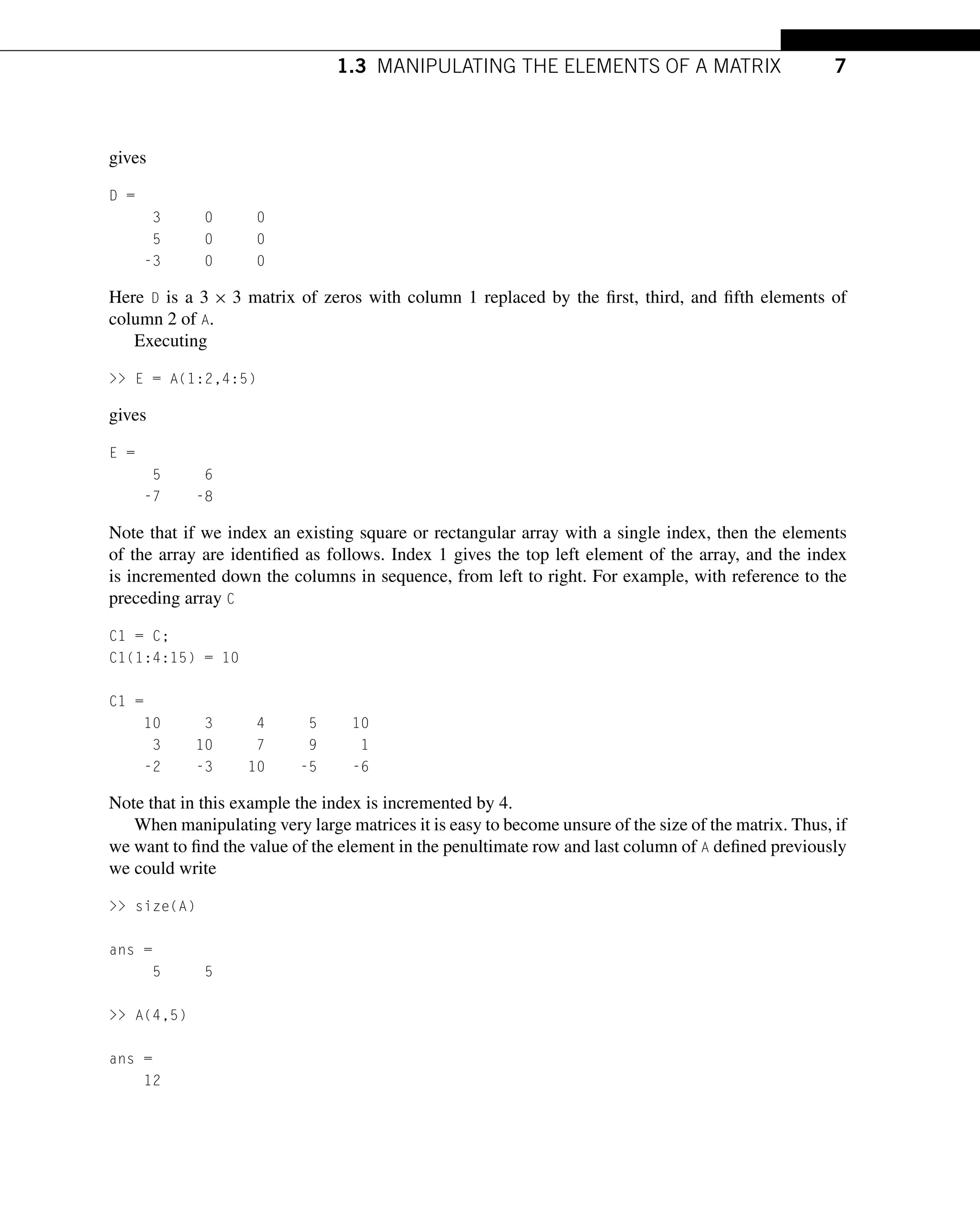
![8 CHAPTER 1 AN INTRODUCTION TO MATLAB®
but it is easier to use end thus:
>> A(end-1,end)
ans =
12
The reshape function may be used to manipulate a matrix. As the name implies, the function reshapes
a given matrix into a new matrix of any specified size provided it has an identical number of elements.
For example a 3 × 4 matrix can be reshaped into a 6 × 2 matrix but a 3 × 3 matrix cannot be reshaped
into a 5 × 2 matrix. It is important to note that this function takes each column of the original matrix in
turn until the new required column size is achieved and then repeats the process for the next column.
For example, consider the matrix P.
>> P = C(:,1:4)
P =
2 3 4 5
3 5 7 9
-2 -3 -4 -5
>> reshape(P,6,2)
ans =
2 4
3 7
-2 -4
3 5
5 9
-3 -5
>> s = reshape(P,1,12);
>> s(1:10)
ans =
2 3 -2 3 5 -3 4 7 -4 5
1.4 TRANSPOSING MATRICES
A simple operation that may be performed on a matrix is transposition which interchanges rows and
columns. Transposition of a vector is briefly discussed in Section 1.2. In MATLAB transposition is
denoted by the symbol ’. For example, consider the matrix A, where
>> A = [1 2 3;4 5 6;7 8 9]](https://image.slidesharecdn.com/24767507-250514105302-3e6bf2cb/75/Numerical-Methods-4th-Edition-George-Lindfield-John-Penny-29-2048.jpg)
![1.5 SPECIAL MATRICES 9
A =
1 2 3
4 5 6
7 8 9
To assign the transpose of A to B we write
>> B = A’
B =
1 4 7
2 5 8
3 6 9
Had we used .’ to obtain the transpose we would have obtained the same result. However, if A is
complex then the MATLAB operator ’ gives the complex conjugate transpose. For example
>> A = [1+2i 3+5i;4+2i 3+4i]
A =
1.0000 + 2.0000i 3.0000 + 5.0000i
4.0000 + 2.0000i 3.0000 + 4.0000i
>> B = A’
B =
1.0000 - 2.0000i 4.0000 - 2.0000i
3.0000 - 5.0000i 3.0000 - 4.0000i
To provide the transpose without conjugation we execute
>> C = A.’
C =
1.0000 + 2.0000i 4.0000 + 2.0000i
3.0000 + 5.0000i 3.0000 + 4.0000i
1.5 SPECIAL MATRICES
Certain matrices occur frequently in matrix manipulations and MATLAB ensures that these are gen-
erated easily. Some of the most common are ones(m,n), zeros(m,n), rand(m,n), randn(m,n), and
randi(p,m,n). These MATLAB functions generate m × n matrices composed of ones, zeros, uni-
formly distributed random numbers, normally distributed random numbers and uniformly distributed
random integers, respectively. In the case of randi(p,m,n), p is the maximum integer. If only a sin-
gle scalar parameter is given, then these statements generate a square matrix of the size given by the](https://image.slidesharecdn.com/24767507-250514105302-3e6bf2cb/75/Numerical-Methods-4th-Edition-George-Lindfield-John-Penny-30-2048.jpg)
![10 CHAPTER 1 AN INTRODUCTION TO MATLAB®
parameter. The MATLAB function eye(n) generates the n × n unit matrix. The function eye(m,n)
generates a matrix of m rows and n columns with a diagonal of ones; thus:
>> A = eye(3,4), B = eye(4,3)
A =
1 0 0 0
0 1 0 0
0 0 1 0
B =
1 0 0
0 1 0
0 0 1
0 0 0
If we wish to generate a random matrix C of the same size as an already existing matrix A, then the
statement C = rand(size(A)) can be used. Similarly D = zeros(size(A)) and E = ones(size(A))
generates a matrix D of zeros and a matrix E of ones, both of which are the same size as matrix A.
Some special matrices with more complex features are introduced in Chapter 2.
1.6 GENERATING MATRICES AND VECTORS WITH SPECIFIED ELEMENT
VALUES
Here we confine ourselves to some relatively simple examples thus:
x = -8:1:8 (or x = -8:8) sets x to a vector having elements −8,−7,...,7,8.
y = -2:.2:2 sets y to a vector having elements −2,−1.8,−1.6,...,1.8,2.
z = [1:3 4:2:8 10:0.5:11] sets z to a vector having the elements
[1 2 3 4 6 8 10 10.5 11]
The MATLAB function linspace also generates a vector. However, in this function the user defines the
beginning and end values of the vector and the number of elements in the vector. For example
>> w = linspace(-2,2,5)
w =
-2 -1 0 1 2
This is simple and could just as well have been created by w = -2:1:2 or even w = -2:2. However,
consider
>> w = linspace(0.2598,0.3024,5)
w =
0.2598 0.2704 0.2811 0.2918 0.3024](https://image.slidesharecdn.com/24767507-250514105302-3e6bf2cb/75/Numerical-Methods-4th-Edition-George-Lindfield-John-Penny-31-2048.jpg)
![1.6 GENERATING MATRICES AND VECTORS 11
Generating this sequence of values by other means would be more difficult. If we require logarithmic
spacing then we can use
>> w = logspace(1,2,5)
w =
10.0000 17.7828 31.6228 56.2341 100.0000
Note that the values produced are between 101 and 102, not 1 and 2. Again, generating these values
by any other means would require some thought! The user of logspace should be warned that if the
second parameter is pi the values run to π, not 10π . Consider the following
>> w = logspace(1,pi,5)
w =
10.0000 7.4866 5.6050 4.1963 3.1416
More complicated matrices can be generated by combining other matrices. For example, consider the
two statements
>> C = [2.3 4.9; 0.9 3.1];
>> D = [C ones(size(C)); eye(size(C)) zeros(size(C))]
These two statements generate a new matrix D the size of which is double the row and column size of
the original C; thus
D =
2.3000 4.9000 1.0000 1.0000
0.9000 3.1000 1.0000 1.0000
1.0000 0 0 0
0 1.0000 0 0
The MATLAB function repmat replicates a given matrix a required number of times. For example,
assuming the matrix C is defined in the preceding statement, then
>> E = repmat(C,2,3)
replicates C as a block to give a matrix with twice as many rows and three times as many columns.
Thus we have a matrix E of 4 rows and 6 columns:
E =
2.3000 4.9000 2.3000 4.9000 2.3000 4.9000
0.9000 3.1000 0.9000 3.1000 0.9000 3.1000
2.3000 4.9000 2.3000 4.9000 2.3000 4.9000
0.9000 3.1000 0.9000 3.1000 0.9000 3.1000
The MATLAB function diag allows us to generate a diagonal matrix from a specified vector of diagonal
elements. Thus](https://image.slidesharecdn.com/24767507-250514105302-3e6bf2cb/75/Numerical-Methods-4th-Edition-George-Lindfield-John-Penny-32-2048.jpg)
![12 CHAPTER 1 AN INTRODUCTION TO MATLAB®
>> H = diag([2 3 4])
generates
H =
2 0 0
0 3 0
0 0 4
There is a second used of the function diag which is to obtain the elements on the leading diagonal of
a given matrix. Consider
>> P = rand(3,4)
P =
0.3825 0.9379 0.2935 0.8548
0.4658 0.8146 0.2502 0.3160
0.1030 0.0296 0.5830 0.6325
then
>> diag(P)
ans =
0.3825
0.8146
0.5830
A more complicated form of diagonal matrix is the block diagonal matrix. This type of matrix can be
generated using the MATLAB function blkdiag. We set matrices A1 and A2 as follows:
>> A1 = [1 2 5;3 4 6;3 4 5];
>> A2 = [1.2 3.5,8;0.6 0.9,56];
Then,
>> blkdiag(A1,A2,78)
ans =
1.0000 2.0000 5.0000 0 0 0 0
3.0000 4.0000 6.0000 0 0 0 0
3.0000 4.0000 5.0000 0 0 0 0
0 0 0 1.2000 3.5000 8.0000 0
0 0 0 0.6000 0.9000 56.0000 0
0 0 0 0 0 0 78.0000
The preceding functions can be very useful in allowing the user to create matrices with complicated
structures, without detailed programming.](https://image.slidesharecdn.com/24767507-250514105302-3e6bf2cb/75/Numerical-Methods-4th-Edition-George-Lindfield-John-Penny-33-2048.jpg)
![1.7 MATRIX ALGEBRA IN MATLAB 13
1.7 MATRIX ALGEBRA IN MATLAB
The matrix is fundamental to MATLAB and we have provided a broad and simple introduction to
matrices in Appendix A.
MATLAB allows matrix equations to be simply expressed and evaluated. For example, to illustrate
matrix addition, subtraction, multiplication, and scalar multiplication, consider the evaluation of the
matrix equation
Z = AAT
+ sP − Q
where s = 0.5 and
A =
2 3 4 5
2 4 6 8
P =
1 3
2 −9
Q =
−7 3
5 1
Assigning A, P, Q, and s, and evaluating this equation in MATLAB we have
A = [2 3 4 5;2 4 6 8];
P = [1 3;2 -9];
Q = [-7 3;5 1];
s = 0.5;
Z = A*A’+s*P-Q
Z =
61.5000 78.5000
76.0000 114.5000
This result can be readily checked by hand!
MATLAB allows a single scalar value to be added to or subtracted from every element of a matrix.
This is called explicit expansion. To illustrate this we first generate a fourth-order Riemann matrix
using the MATLAB function gallery. This function gives the user access to a range of special matrices
with useful properties. See Chapter 2 for further discussion. In the following piece of MATLAB code
we use it to generate a 4 × 4 Riemann matrix, and then subtract 0.5 from every element of the matrix.
R = gallery(’riemann’,4)
R =
1 -1 1 -1
-1 2 -1 -1
-1 -1 3 -1
-1 -1 -1 4
A = R-0.5
A =
0.5000 -1.5000 0.5000 -1.5000
-1.5000 1.5000 -1.5000 -1.5000
-1.5000 -1.5000 2.5000 -1.5000
-1.5000 -1.5000 -1.5000 3.5000](https://image.slidesharecdn.com/24767507-250514105302-3e6bf2cb/75/Numerical-Methods-4th-Edition-George-Lindfield-John-Penny-34-2048.jpg)
![14 CHAPTER 1 AN INTRODUCTION TO MATLAB®
In the 2016b release of MATLAB this feature has been extended to allow a row or column vector to be
added to a matrix. For example
B = 2*ones(4)-[1 2 3 4]
B =
1 0 -1 -2
1 0 -1 -2
1 0 -1 -2
1 0 -1 -2
C = 2*ones(4)+[2 4 6 8]’
C =
4 4 4 4
6 6 6 6
8 8 8 8
10 10 10 10
Note that 2*ones(4) produces a 4 × 4 matrix where each element is 2. In computing B the results
show that 1 is subtracted from each element of the first column, the 2 from each element in the second
column, the 3 from each element of the third column and so on. Similarly. in computing C the results
show that 2 is added to each element of the first row, the 4 to each element in the second row, the 6 to
each element of the third row and so on.
1.8 MATRIX FUNCTIONS
Some arithmetic operations are simple to evaluate for single scalar values but involve a great deal of
computation for matrices. For large matrices such operations may take a significant amount of time.
An example of this is where a matrix is raised to a power. We can write this in MATLAB as A^p where
p is a scalar value and A is a square matrix. This produces the power of the matrix for any value of p. For
the case where the power equals 0.5 it is better to use sqrtm(A) which gives the principal square root
of the matrix A, (see Appendix A, Section A.13). Similarly, for the case where the power equals −1
it is better to use inv(A). Another special operation directly available in MATLAB is expm(A) which
gives the exponential of the matrix A. The MATLAB function logm(A) provides the principal logarithm
to the base e of A. If B=logm(A) then the principal logarithm B is the unique logarithm for which every
eigenvalue has an imaginary part lying strictly between −π and π.
For example
A = [61 45;60 76]
A =
61 45
60 76](https://image.slidesharecdn.com/24767507-250514105302-3e6bf2cb/75/Numerical-Methods-4th-Edition-George-Lindfield-John-Penny-35-2048.jpg)
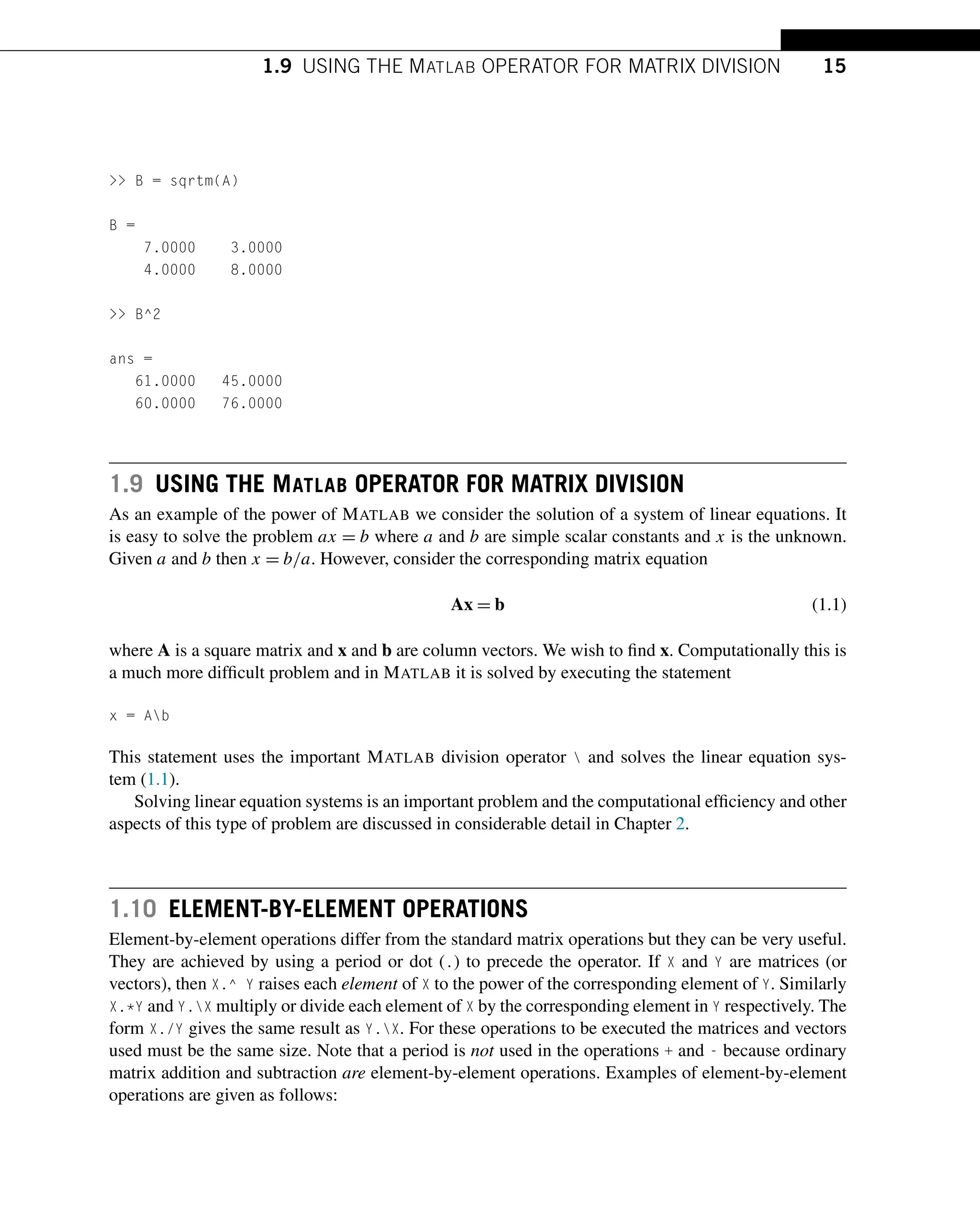
![16 CHAPTER 1 AN INTRODUCTION TO MATLAB®
A = [1 2;3 4]
A =
1 2
3 4
B = [5 6;7 8]
B =
5 6
7 8
First we use normal matrix multiplication thus:
A*B
ans =
19 22
43 50
However, using the dot operator (.) we have
A.*B
ans =
5 12
21 32
which is element-by-element multiplication. Now consider the statement
A.^B
ans =
1 64
2187 65536
In the above, each element of A is raised to the corresponding power in B.
Element-by-element operations have many applications. An important use is in plotting graphs (see
Section 1.14). For example
x = -1:0.1:1;
y = x.*cos(x);
y1 = x.^3.*(x.^2+3*x+sin(x));
Notice here that using the vector x of many values, allows a vector of corresponding values for y and
y1 to be computed simultaneously from single statements. Element-by-element operations are in effect
operations on scalar quantities performed simultaneously.](https://image.slidesharecdn.com/24767507-250514105302-3e6bf2cb/75/Numerical-Methods-4th-Edition-George-Lindfield-John-Penny-37-2048.jpg)
![1.11 SCALAR OPERATIONS AND FUNCTIONS 17
1.11 SCALAR OPERATIONS AND FUNCTIONS
In MATLAB we can define and manipulate scalar quantities, as in most other computer languages, but
no distinction is made in the naming of matrices and scalars. Thus A could represent a scalar or matrix
quantity. The process of assignment makes the distinction. For example
x = 2;
y = x^2+3*x-7
y =
3
x = [1 2;3 4]
x =
1 2
3 4
y = x.^2+3*x-7
y =
-3 3
11 21
Note that in the preceding examples, when vectors are used the dot must be placed before the operator.
This is not required for scalar operations, but does not cause errors if used.
In the case where we multiply a square matrix by itself, for example, in the form x^2 we get the
full matrix multiplication as shown below, rather than element-by-element multiplication as given by
x.^2.
y = x^2+3*x-7
y =
3 9
17 27
A very large number of mathematical functions are directly built into MATLAB. They act on scalar
quantities, arrays or vectors on an element-by-element basis. They may be called by using the function
name together with the parameters that define the function. These functions may return one or more
values. A small selection of MATLAB functions is given in the following table which lists the function
name, the function use and an example function call. Note that all function names must be in lower
case letters.
All MATLAB functions are not listed in Table 1.1, but MATLAB provides a complete range of
trigonometric and inverse trigonometric functions, hyperbolic and inverse hyperbolic functions and](https://image.slidesharecdn.com/24767507-250514105302-3e6bf2cb/75/Numerical-Methods-4th-Edition-George-Lindfield-John-Penny-38-2048.jpg)
![18 CHAPTER 1 AN INTRODUCTION TO MATLAB®
Table 1.1 Selected MATLAB mathematical functions
Function Function gives Example
sqrt(x) square root of x y = sqrt(x+2.5);
abs(x) if x is real, is the positive value of x
if x is complex, is the scalar measure of x d = abs(x)*y;
real(x) real part of x when x is complex d = real(x)*y;
imag(x) imaginary part of x when x is complex d = imag(x)*y;
conj(x) the complex conjugate of x x = conj(y);
sin(x) sine of x in radians t = x+sin(x);
asin(x) inverse sine of x returned in radians t = x+sin(x);
sind(x) sine of x in degrees t = x+sind(x);
log(x) log to base e of x z = log(1+x);
log10(x) log to base 10 of x z = log10(1-2*x);
cosh(x) hyperbolic cosine of x u = cosh(pi*x);
exp(x) exponential of x, i.e., ex p = .7*exp(x);
gamma(x) gamma function of x f = gamma(y);
bessel(n,x) nth-order Bessel function of x f = bessel(2,y);
logarithmic functions. The following examples illustrate the use of some of the functions listed be-
fore:
x = [-4 3];
abs(x)
ans =
4 3
x = 3+4i;
abs(x)
ans =
5
imag(x)
ans =
4
y = sin(pi/4)
y =
0.7071
and](https://image.slidesharecdn.com/24767507-250514105302-3e6bf2cb/75/Numerical-Methods-4th-Edition-George-Lindfield-John-Penny-39-2048.jpg)
![1.11 SCALAR OPERATIONS AND FUNCTIONS 19
x = linspace(0,pi,5)
x =
0 0.7854 1.5708 2.3562 3.1416
sin(x)
ans =
0 0.7071 1.0000 0.7071 0.0000
and
x = [0 pi/2;pi 3*pi/2]
x =
0 1.5708
3.1416 4.7124
y = sin(x)
y =
0 1.0000
0.0000 -1.0000
Some functions perform special calculations for important and general mathematical processes. These
functions often require more than one input parameter and may provide several outputs. For example,
bessel(n,x) gives the nth-order Bessel function of x. The statement y = fzero(’fun’,x0) deter-
mines the root of the function fun near to x0 where fun is a function defined by the user that provides
the equation for which we are finding the root. For examples of the use of fzero, see Section 3.1. The
statement [Y,I] = sort(X) is an example of a function that can return two output values. Y is the
sorted matrix and I is a matrix containing the indices of the sort.
In addition to a large number of mathematical functions, MATLAB provides several utility functions
that may be used for examining the operation of scripts. These are:
pause causes the execution of the script to pause until the user presses a key. Note that the cursor is
turned into the symbol P, warning the script is in pause mode. This is often used when the script
is operating with echo on.
echo on displays each line of script in the command window before execution. This is useful for
demonstrations. To turn it off, use the statement echo off.
who lists the variables in the current workspace.
whos lists all the variables in the current workspace, together with information about their size and
class, and so on.
MATLAB also provides functions related to time:](https://image.slidesharecdn.com/24767507-250514105302-3e6bf2cb/75/Numerical-Methods-4th-Edition-George-Lindfield-John-Penny-40-2048.jpg)
![20 CHAPTER 1 AN INTRODUCTION TO MATLAB®
clock returns the current date and time in the form: year month day hour min sec.
etime(t2,t1) calculates elapsed time between t1 and t2. Note that t1 and t2 are output from the
clock function. When timing the duration of an event tic ... toc should be used.
tic ... toc times an event. For example, finding the time taken to execute a segment of script. The
statement tic starts the timing and toc gives the elapsed time since the last tic.
cputime returns the total time in seconds since MATLAB was launched.
timeit times the operation of a function. Suppose we carry out a 8192 point Fourier
transform using the MATLAB function fft (described in Chapter 8) then we run
fft_time = timeit(@()fft(8192)).
The script e4s101.m uses the timing functions described previously to estimate the time taken to solve
a 1000 × 1000 system of linear equations:
% e4s101.m Solves a 5000 x 5000 linear equation system
A = rand(5000); b = rand(5000,1);
T_before = clock;
tic
t0 = cputime;
y = Ab;
tend = toc;
t1 = cputime-t0;
t2 = timeit(@() Ab);
disp(’ tic-toc cputime timeit’)
fprintf(’%10.2f %10.2f %10.2f nn’, tend,t1,t2)
Running script e4s101.m on a particular computer gave the following results:
tic-toc cputime timeit
2.52 5.09 2.60
The output shows that the three alternative methods of timing give essentially the same value. When
measuring computing times the displayed times vary from run to run and the shorter the run time, the
greater the percentage variation.
1.12 STRING VARIABLES
We have found that MATLAB makes no distinction in naming matrices and scalar quantities. This is
also true of string variables or strings. For example, A = [1 2; 3 4], A = 17.23, or A = ’help’ are
each valid statements and assign an array, a scalar or a text string respectively to A.
Characters and strings of characters can be assigned to variables directly in MATLAB by placing the
string in quotes and then assigning it to a variable name. Strings can then be manipulated by specific
MATLAB string functions which we list in this section. Some examples showing the manipulation of
strings using standard MATLAB assignment are given below.](https://image.slidesharecdn.com/24767507-250514105302-3e6bf2cb/75/Numerical-Methods-4th-Edition-George-Lindfield-John-Penny-41-2048.jpg)
![1.12 STRING VARIABLES 21
s1 = ’Matlab ’, s2 = ’is ’, s3 = ’useful’
s1 =
Matlab
s2 =
is
s3 =
useful
Strings in MATLAB are represented as vectors of the equivalent ASCII code numbers; it is only the
way that we assign and access them that makes them strings. For example, the string ’is ’ is actually
saved as the vector [105 115 32]. Hence, we can see that the ASCII codes for the letters i, s, and
a space are 105, 115, and 32 respectively. This vector structure has important implications when we
manipulate strings. For example, we can concatenate strings, because of their vector nature, by using
the square brackets as follows
sc = [s1 s2 s3]
sc =
Matlab is useful
Note the spaces are recognized. To identify any item in the string array we can write:
sc(2)
ans =
a
To identify a subset of the elements of this string we can write:
sc(3:10)
ans =
tlab is
we can display a string vertically, by transposing the string vector thus:
sc(1:3)’
ans =
M
a
t
We can also reverse the order of a substring and assign it to another string as follows:](https://image.slidesharecdn.com/24767507-250514105302-3e6bf2cb/75/Numerical-Methods-4th-Edition-George-Lindfield-John-Penny-42-2048.jpg)
![22 CHAPTER 1 AN INTRODUCTION TO MATLAB®
a = sc(6:-1:1)
a =
baltaM
We can define string arrays as well. For example, using the string sc as defined previously:
sd = ’Numerical method’
s = [sc; sd]
Matlab is useful
Numerical method
To obtain the 12th column of this string we use
s(:,12)
ans =
s
e
Note that the string lengths must be the same in order to form a rectangular array of ASCII code
numbers. In this case the array is 2 × 16. We now show how MATLAB string functions can be used to
manipulate strings. To replace one string by another we use strrep as follows:
strrep(sc,’useful’,’super’)
ans =
Matlab is super
Notice that this statement causes useful in sc to be replaced by super.
We can determine if a particular character or string is present in another string by using findstr.
For example
findstr(sd,’e’)
ans =
4 12
This tells us that the 4th and 12th characters in the string are ‘e’. We can also use this function to find
the location of a substring of this string as follows
findstr(sd, ’meth’)
ans =
11
The string ’meth’ begins at the 11th character in the string. If the substring or character is not in the
original string, we have the result illustrated by the example below:](https://image.slidesharecdn.com/24767507-250514105302-3e6bf2cb/75/Numerical-Methods-4th-Edition-George-Lindfield-John-Penny-43-2048.jpg)
![1.12 STRING VARIABLES 23
findstr(sd,’E’)
ans =
[ ]
We can convert a string to its ASCII code equivalent by either using the function double or by invoking
any arithmetic operation. Thus, operating on the existing string sd we have
p = double(sd(1:9))
p =
78 117 109 101 114 105 99 97 108
q = 1*sd(1:9)
q =
78 117 109 101 114 105 99 97 108
Note that in the case where we are multiplying the string by 1, MATLAB treats the string as a vector
of ASCII equivalent numbers and multiplies it by 1. Recalling that sd(1:9) = ’Numerical ’ we can
deduce that the ASCII code for N is 78 and for u it is 117, etc.
We convert a vector of ASCII code to a string using the MATLAB char function. For example
char(q)
ans =
Numerical
To increase each ASCII code number by 3, and then to convert to the character equivalent we have
char(q+3)
ans =
Qxphulfdo
char((q+3)/2)
ans =
(84:6327
double(ans)
ans =
40 60 56 52 58 54 51 50 55
char(q) has converted the ASCII string back to characters. Here we have shown that it is possible to do
arithmetic on the ASCII code numbers and, if we wish, convert back to characters. If after manipulation
the ASCII code values are non-integer, they are rounded down.
It is important to appreciate that the string ‘123’ and the number 123 are not the same. Thus](https://image.slidesharecdn.com/24767507-250514105302-3e6bf2cb/75/Numerical-Methods-4th-Edition-George-Lindfield-John-Penny-44-2048.jpg)
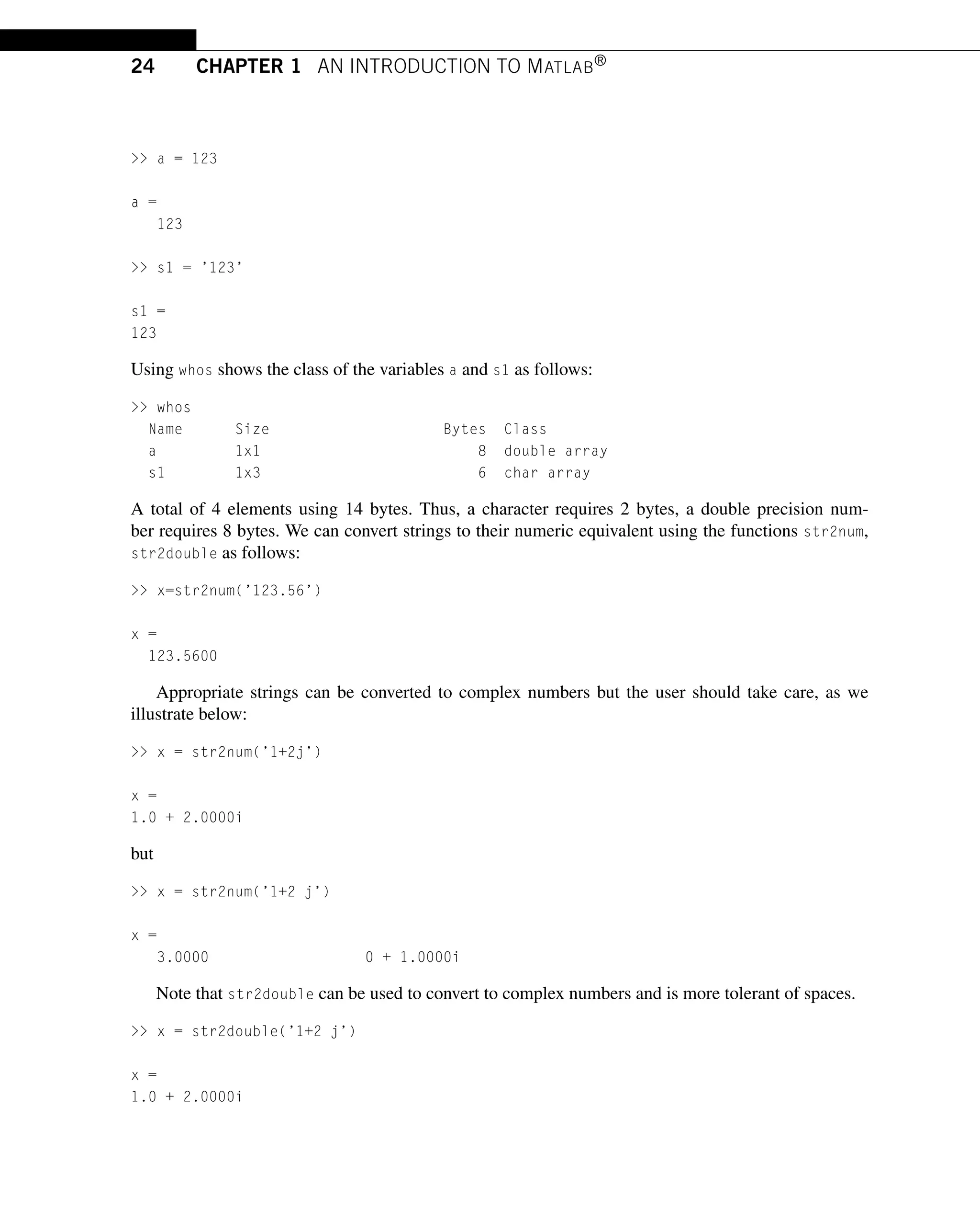
![1.13 INPUT AND OUTPUT IN MATLAB 25
There are many MATLAB functions which are available to manipulate strings; see the appropriate
MATLAB manual. Here we illustrate the use of some functions.
bin2dec(’111001’) or bin2dec(’111 001’) returns 57.
dec2bin(57) returns the string ‘111001’.
int2str([3.9 6.2]) returns the string ‘4 6’.
num2str([3.9 6.2]) returns the string ‘3.9 6.2’.
str2num(’3.9 6.2’) returns 3.9000 6.2000.
strcat(’how ’,’why ’,’when’) returns the string ‘howwhywhen’.
strcmp(’whitehouse’,’whitepaint’) returns 0 because strings are not identical.
strncmp(’whitehouse’,’whitepaint’,5) returns 1 because first the 5 characters of strings are
identical.
date returns the current date, in the form 24-Aug-2011.
A useful and common application of the function num2str is in the disp and title functions see
Sections 1.13 and 1.14 respectively.
1.13 INPUT AND OUTPUT IN MATLAB
To output the names and values of variables, the semicolon can be omitted from assignment statements.
However, this does not produce clear scripts or well-organized and tidy output. It is often better practice
to use the function disp since this leads to clearer scripts. The disp function allows the display of text
and values on the screen. To output the contents of the matrix A on the screen we write disp(A). Text
output must be placed in single quotes, for example,
disp(’This will display this test’)
This will display this test
Combinations of strings can be printed using square brackets [ ], and numerical values can be placed
in text strings if they are converted to strings using the num2str function. For example,
x = 2.678;
disp([’Value of iterate is ’, num2str(x), ’ at this stage’])
will place on the screen
Value of iterate is 2.678 at this stage
The more flexible fprintf function allows formatted output to the screen or to a file. It takes the
form
fprintf(’filename’,’format_string’,list);
Here list is a list of variable names separated by commas. The filename parameter is optional; if not
present, output is to the screen rather than to the filename. The format string formats the output. The
basic elements that may be used in the format string are](https://image.slidesharecdn.com/24767507-250514105302-3e6bf2cb/75/Numerical-Methods-4th-Edition-George-Lindfield-John-Penny-46-2048.jpg)
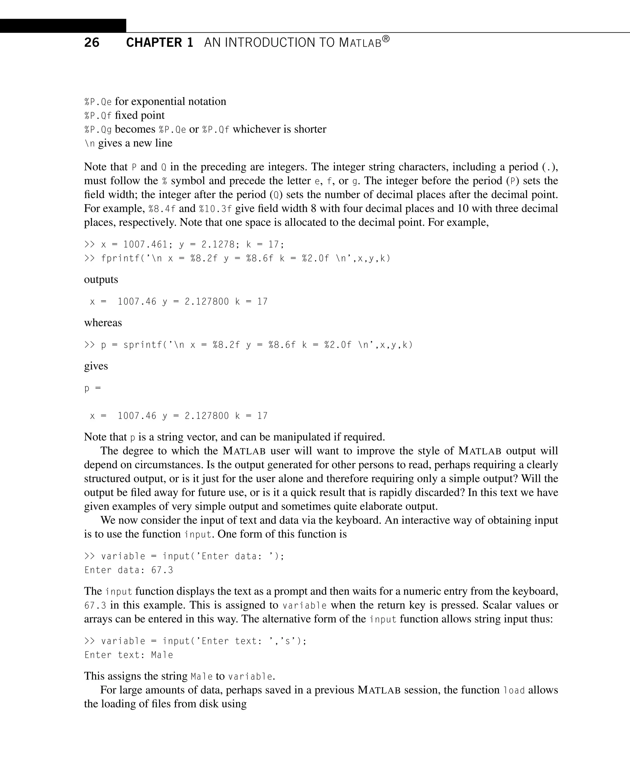
![28 CHAPTER 1 AN INTRODUCTION TO MATLAB®
using csvread. We use csvwrite to generate a CSV file from MATLAB. In the following MATLAB
statements we save the vector p, we clear the workspace and then reload p, but now call it the vector g:
p = 1:6;
whos
Name Size Bytes Class
p 1x6 48 double array
csvwrite(’test003’,p)
clear
g = csvread(’test003’)
g =
1 2 3 4 5
As a further example of the load and save commands, consider the following example:
% e4s110
x = [1 0 2 3 1]; y = [-1 0 4 1 1];
A = [x;x.^2; x.^3;x.^4;x.^5];
B = [x;2*x; 3*x; 4*x;5*x];
save test004 A B
clear all
whos
disp(’nothing listed’)
load test004
C = A*B;
disp(’Results of matrix multiplication’)
disp(C)
Running script e4s110 gives
e4s110
nothing listed
Results of matrix multiplication
24 0 48 72 24
54 0 108 162 54
138 0 276 414 138
378 0 756 1134 378
1074 0 2148 3222 1074
1.14 MATLAB GRAPHICS
MATLAB provides a wide range of graphics facilities which may be called from within a script or
used simply in command mode for direct execution. We begin by considering the plot function. This
function takes several forms. For example,](https://image.slidesharecdn.com/24767507-250514105302-3e6bf2cb/75/Numerical-Methods-4th-Edition-George-Lindfield-John-Penny-49-2048.jpg)
![1.14 MATLAB GRAPHICS 29
Table 1.2 Symbols and characters used in plotting
Line Symbol Point Symbol Color Character
Solid - point . yellow y
Dashed - - plus + red r
Dotted : star * green g
Dashdot -. circle o blue b
x mark × black k
plot(x,y) plots the vector x against y. If x and y are matrices the first column of x is plotted against
the first column of y. This is then repeated for each pair of columns of x and y.
plot(x1,y1,’type1’,x2,y2,’type2’) plots the vector x1 against y1 using the line or point type given
by type1, and the vector x2 against y2 using the line or point type given by type2.
The type is selected by using the required symbol from Table 1.2. This symbol may be preceded by a
character indicating a color.
Semilog and log–log graphs can be obtained by replacing plot by semilogx, semilogy, or loglog
functions and various other replacements for plot are available to give special plots. Titles, axis labels
and other features can be added to a given graph using the functions xlabel, ylabel, title, grid, and
text. These functions have the following forms:
title(’title’) displays the title which is enclosed between quotes, at the top of the graph.
xlabel(’x_axis_name’) displays the name which is enclosed between quotes for the x-axis.
ylabel(’y_axis_name’) displays the name which is enclosed between quotes for the y-axis.
grid superimposes a grid on the graph.
text(x,y,’text-at-x,y’) displays text at position (x, y) in the graphics window where x and y are
measured in the units of the current plotting axes. There may be one point or many at which text is
placed depending on whether or not x and y are vectors.
gtext(’text’) allows the placement of text using the mouse by positioning it where the text is required
and then pressing the mouse button.
ginput allows information to be taken from a graphics window. The function takes two main forms.
The simplest is
[x,y] = ginput
This inputs an unlimited number of points into the vectors x and y by positioning the mouse cross-hairs
at the points required and then pressing the mouse button. To exit ginput the return key must be pressed.
If a specific number of points n are required, then we write
[x,y] = ginput(n)
In addition, the function axis allows the user to set the limits of the axes for a particular plot. This
takes the form axis(p) where p is a four-element row vector specifying the lower and upper limits of
the axes in the x and y directions. The axis statement must be placed after the plot statement to which
it refers. Similarly the functions xlabel, ylabel, title, grid, text, gtext, and axis must follow the
plot to which they refer.
Script e4s102.m gives the plot which is output as Fig. 1.1. The function hold is used to ensure that
the two graphs are superimposed.](https://image.slidesharecdn.com/24767507-250514105302-3e6bf2cb/75/Numerical-Methods-4th-Edition-George-Lindfield-John-Penny-50-2048.jpg)
![30 CHAPTER 1 AN INTRODUCTION TO MATLAB®
FIGURE 1.1
Superimposed graphs obtained using plot(x,y) and hold statements.
% e4s102.m
x = -4:0.05:4;
y = exp(-0.5*x).*sin(5*x);
figure(1), plot(x,y)
xlabel(’x-axis’), ylabel(’y-axis’)
hold on
y = exp(-0.5*x).*cos(5*x);
plot(x,y), grid
gtext(’Two tails...’)
hold off
Script e4s102.m illustrates how few MATLAB statements are required to generate a graph.
The function fplot allows the user to plot a previously defined function between given limits. The
important difference between fplot and plot is that fplot chooses the plotting points in the given
range adaptively depending on the rate of change of the function at that point. Thus, more points
are chosen when the function is changing more rapidly. This is illustrated by executing the MATLAB
script e4s103.m:
% e4s103.m
y = @(x) sin(x.^3);
x = 2:.04:4;
figure(1)
plot(x,y(x),’o-’)
xlabel(’x’), ylabel(’y’)
figure(2)
fplot(y,[2 4])
xlabel(’x’), ylabel(’y’)
Note figure(1) and figure(2) direct the graphic output to separate windows. The interpretation of
the anonymous function @(x) sin(x.^3) is explained in Section 1.19.](https://image.slidesharecdn.com/24767507-250514105302-3e6bf2cb/75/Numerical-Methods-4th-Edition-George-Lindfield-John-Penny-51-2048.jpg)
![1.14 MATLAB GRAPHICS 31
FIGURE 1.2
Plot of y = sin(x3) using 51 equispaced plotting
points.
FIGURE 1.3
Plot of y = sin(x3) using the function fplot to choose
plotting points adaptively.
Running script e4s103.m produces Fig. 1.2 and Fig. 1.3. In the plot example, we have deliberately
chosen an inadequate number of plotting points and this is reflected in the quality of Fig. 1.2. The
function fplot produces a smoother and more accurate curve. Note that fplot only allows a function
or functions to be plotted against an independent variable. Parametric plots cannot be created by fplot.
The MATLAB function ezplot is similar to fplot in the sense that we only have to specify the
function, but has the disadvantage that the step size is fixed. However, ezplot does allow parametric
plots and three-dimensional plots. For example
ezplot(@(t) (cos(3*t)), @(t) (sin(1.6*t)), [0 50])
is a parametric plot but the plot is rather coarse.
We have seen how fplot helps in plotting difficult functions. Other functions which help to clarify
when the plot of a function is unclear or unpredictable are ylim and xlim. The function ylim allows the
user to easily limit the range of the y-axis in the plot and xlim does the same for the x-axis. Their use
is illustrated by the following example. Fig. 1.4 (without the uses of xlim and ylim) is unsatisfactory
since it gives little understanding about how the function behaves except at the specific points x = −2.5,
x = 1, and x = 3.5.
x = -4:0.0011:4;
y =1./(((x+2.5).^2).*((x-3.5).^2))+1./((x-1).^2);
plot(x,y)
ylim([0,10])
Fig. 1.5 shows how the MATLAB statement ylim([0,10]) restricts the y-axis to maximum value
of 10. This gives a clear picture of the behavior of the graph. There are a number of special features
available in MATLAB for the presentation and manipulation of graphs and some of these are now be
discussed. The subplot function takes the form subplot(p,q,r) where p and q split the figure window
into a p × q grid of cells and places the plot in the rth cell of the grid, numbered consecutively along](https://image.slidesharecdn.com/24767507-250514105302-3e6bf2cb/75/Numerical-Methods-4th-Edition-George-Lindfield-John-Penny-52-2048.jpg)
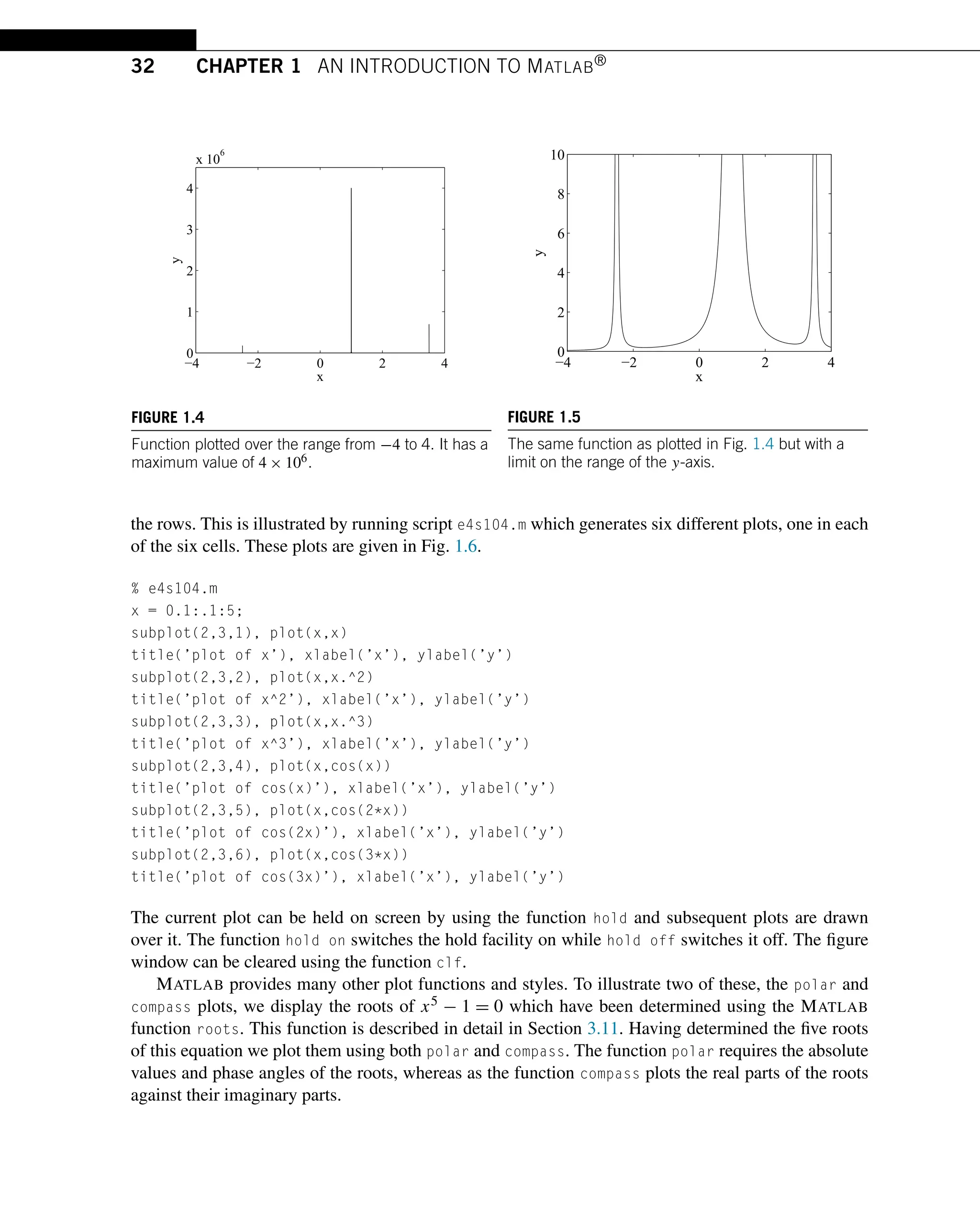
![1.14 MATLAB GRAPHICS 33
FIGURE 1.6
An example of the use of the subplot function.
p=roots([1 0 0 0 0 1])
p =
-1.0000
-0.3090 + 0.9511i
-0.3090 - 0.9511i
0.8090 + 0.5878i
0.8090 - 0.5878i
pm = abs(p.’)
pm =
1.0000 1.0000 1.0000 1.0000 1.0000
pa = angle(p.’)
pa =
3.1416 1.8850 -1.8850 0.6283 -0.6283
subplot(1,2,1), polar(pa,pm,’ok’)
subplot(1,2,2), compass(real(p),imag(p),’k’)
Fig. 1.7 shows these subplots.
An interesting development introduced in the 2016b release of MATLAB are polar scatter and polar
histogram plots that allow data to be plotted in polar coordinates. For the polar scatter function the
points are plotted on a circle, each point being denoted by a circle, or some other selected symbol.](https://image.slidesharecdn.com/24767507-250514105302-3e6bf2cb/75/Numerical-Methods-4th-Edition-George-Lindfield-John-Penny-54-2048.jpg)