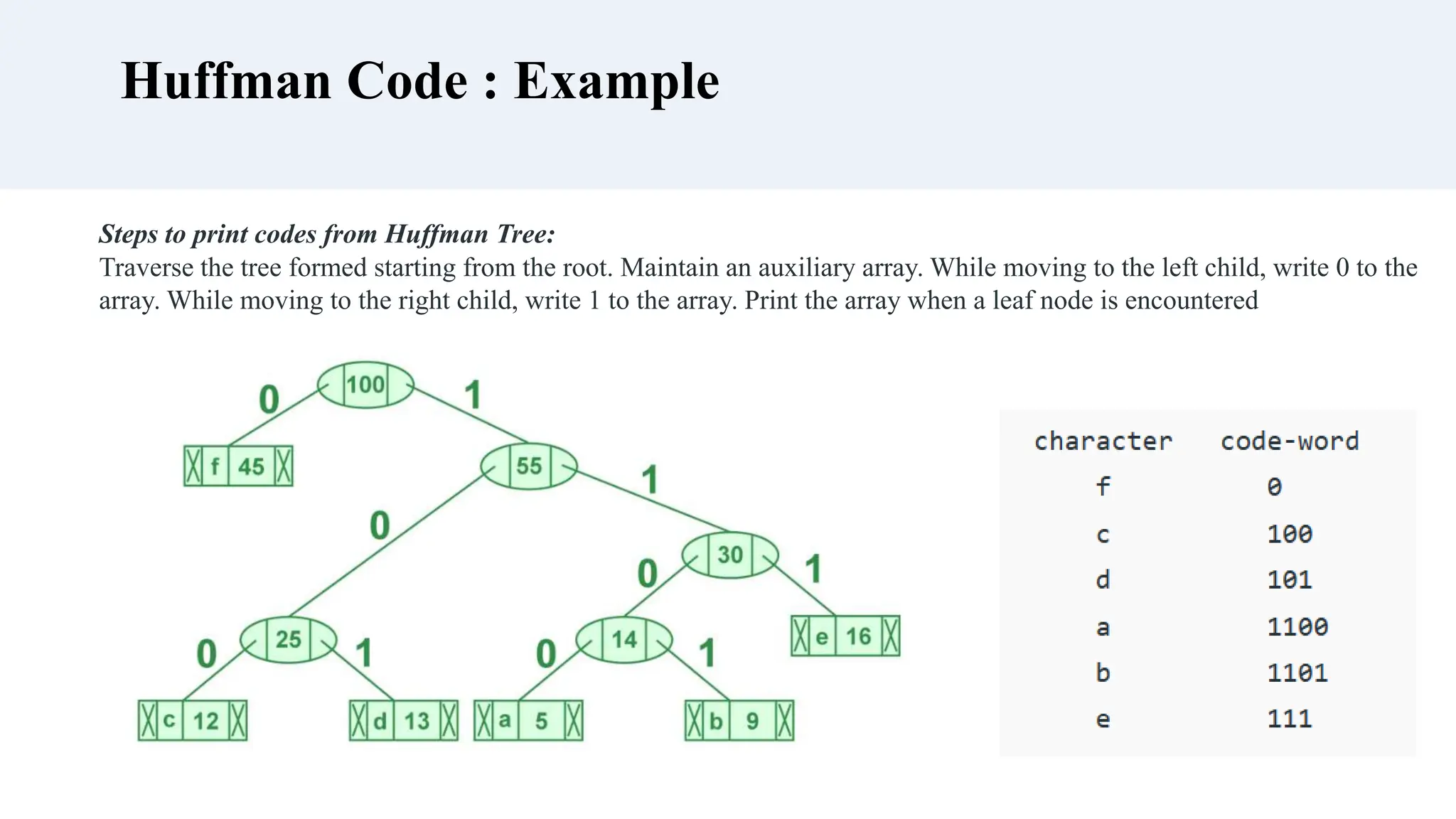
The document summarizes algorithms related to divide and conquer and greedy algorithms. It discusses binary search, finding maximum and minimum, merge sort, quick sort, and Huffman codes. The key steps of divide and conquer algorithms are to divide the problem into subproblems, conquer the subproblems by solving them recursively, and combine the solutions to solve the overall problem. Greedy algorithms make locally optimal choices at each step to find a global optimal solution. Huffman coding assigns variable-length codes to characters based on frequency to compress data.

![Divide and Conquer
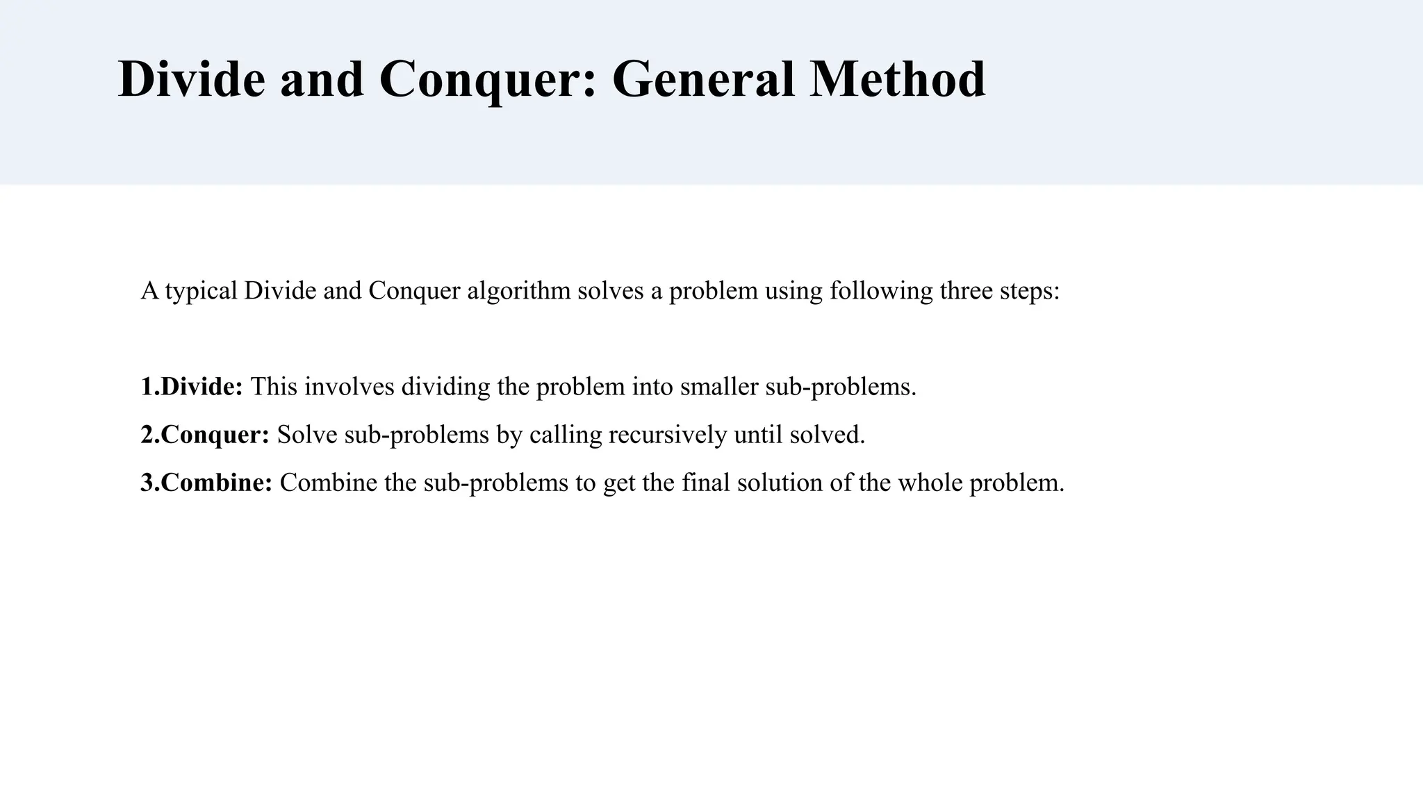
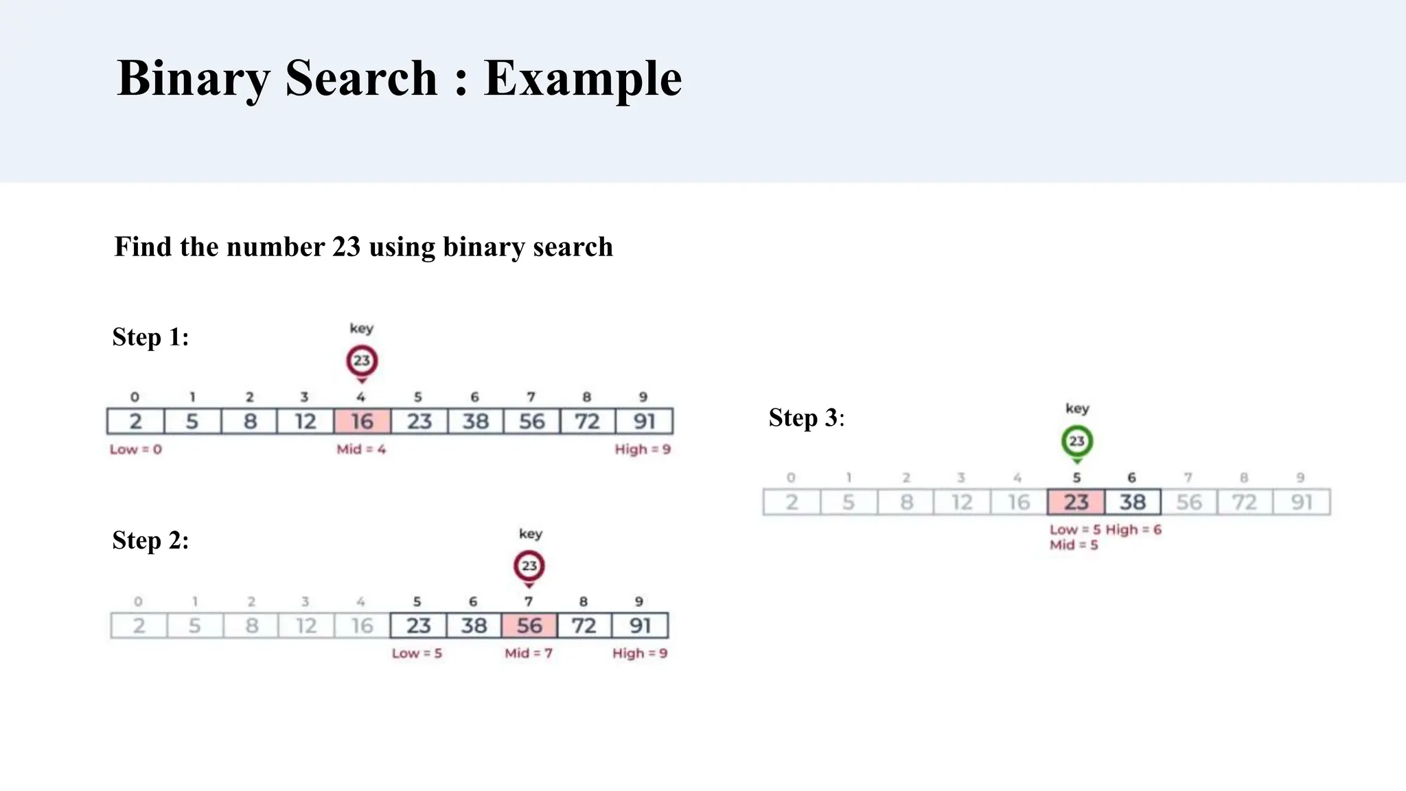
Using the Divide and Conquer technique, we divide a problem into subproblems. When the solution
to each subproblem is ready, we 'combine' the results from the subproblems to solve the main
problem.
Suppose we had to sort an array A. A subproblem would be to sort a sub-section of this array starting
at index p and ending at index r, denoted as A[p..r].
Divide
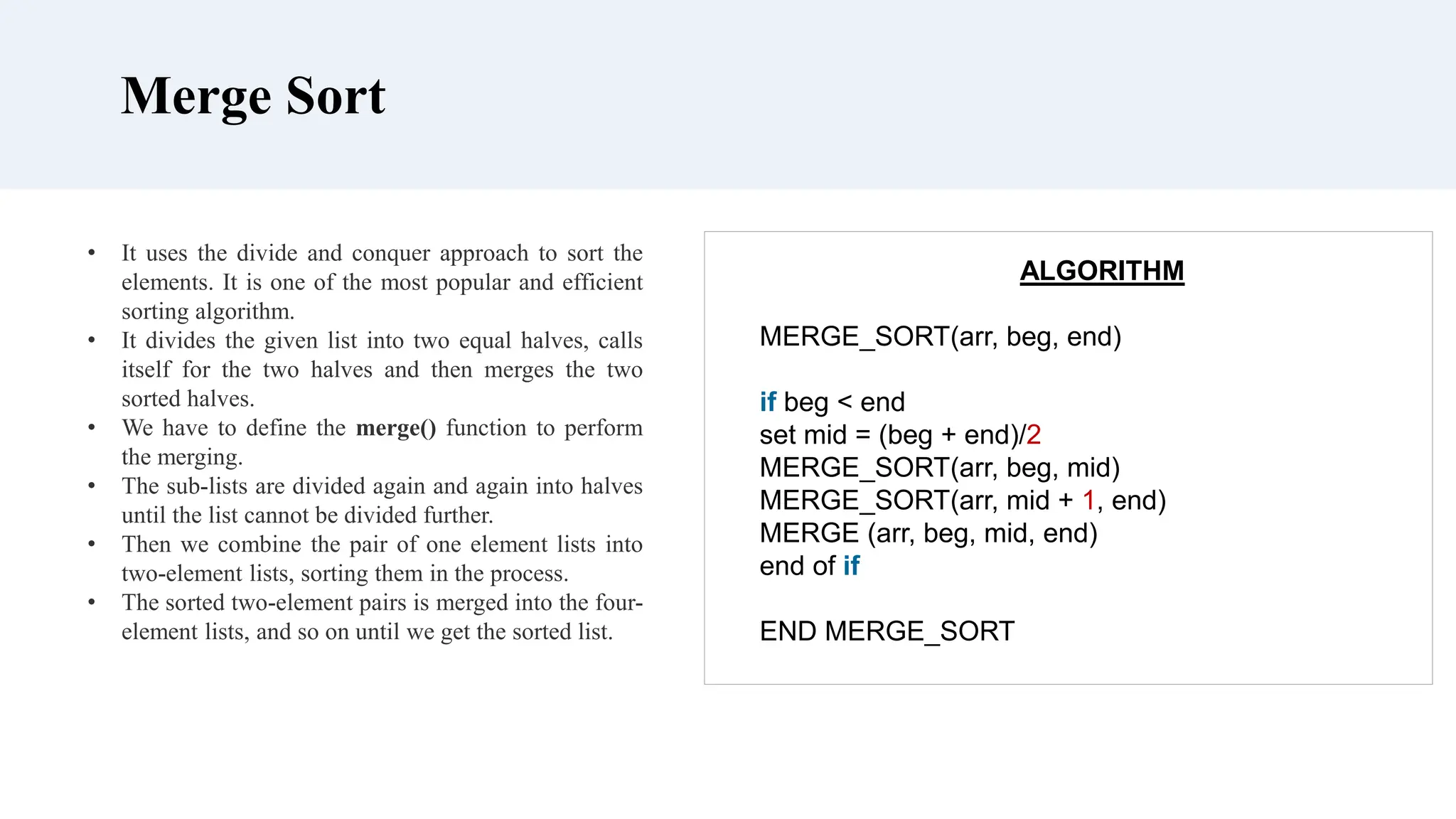
If q is the half-way point between p and r, then we can split the subarray A[p..r] into two
arrays A[p..q] and A[q+1, r].
Conquer
In the conquer step, we try to sort both the subarrays A[p..q] and A[q+1, r]. If we haven't yet reached
the base case, we again divide both these subarrays and try to sort them.
Combine
When the conquer step reaches the base step and we get two sorted subarrays A[p..q] and A[q+1,
r] for array A[p..r], we combine the results by creating a sorted array A[p..r] from two sorted
subarrays A[p..q] and A[q+1, r].](https://image.slidesharecdn.com/daa-unit2-240325042900-457be414/75/Data-analysis-and-algorithms-UNIT-2-pptx-4-2048.jpg)
![void merge(int a[], int beg, int mid, int end)
{
int i, j, k;
int n1 = mid - beg + 1;
int n2 = end - mid;
int LeftArray[n1], RightArray[n2]; //temporary arrays
/* copy data to temp arrays */
for (int i = 0; i < n1; i++)
LeftArray[i] = a[beg + i];
for (int j = 0; j < n2; j++)
RightArray[j] = a[mid + 1 + j];
i = 0, /* initial index of first sub-array */
j = 0; /* initial index of second sub-array */
k = beg; /* initial index of merged sub-array */
while (i < n1 && j < n2)
{
if(LeftArray[i] <= RightArray[j])
{
a[k] = LeftArray[i];
i++;
}
Merge Sort : Algorithm
else
{
a[k] = RightArray[j];
j++;
}
k++;
}
while (i<n1)
{
a[k] = LeftArray[i];
i++;
k++;
}
while (j<n2)
{
a[k] = RightArray[j];
j++;
k++;
}
}](https://image.slidesharecdn.com/daa-unit2-240325042900-457be414/75/Data-analysis-and-algorithms-UNIT-2-pptx-10-2048.jpg)
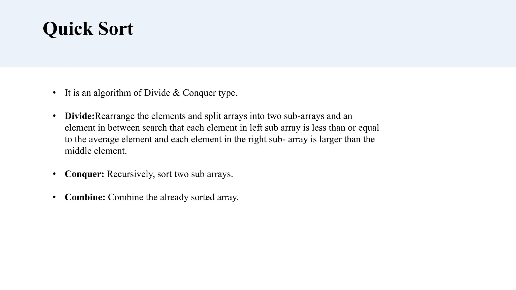
![Quick Sort : Algorithm
function quick_sort(array):
if array is empty:
return array
else:
pivot = array[-1]
less = [x for x in array if x < pivot]
greater = [x for x in array if x >= pivot]
return quick_sort(less) + [pivot] + quick_sort(greater)](https://image.slidesharecdn.com/daa-unit2-240325042900-457be414/75/Data-analysis-and-algorithms-UNIT-2-pptx-13-2048.jpg)

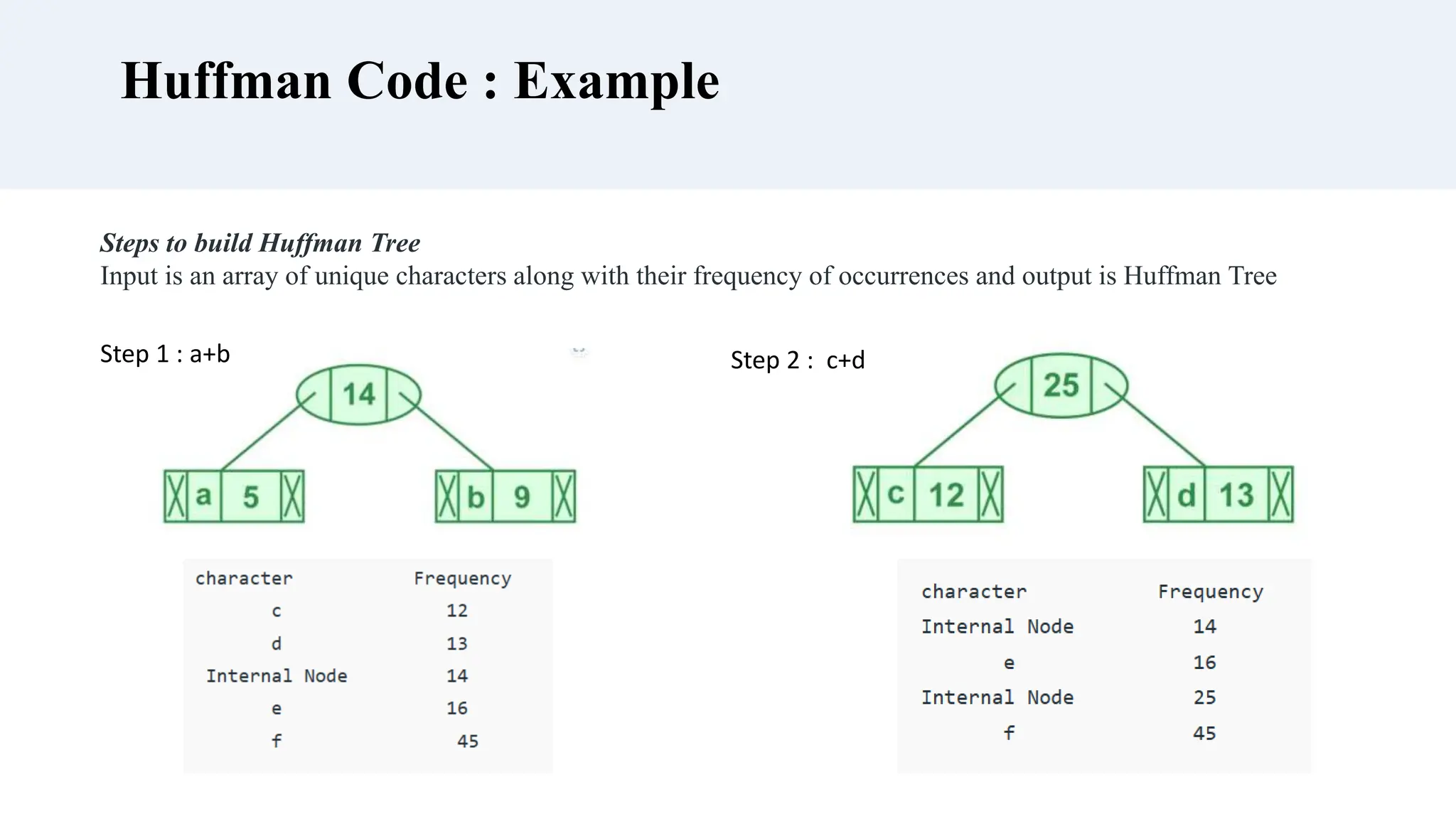
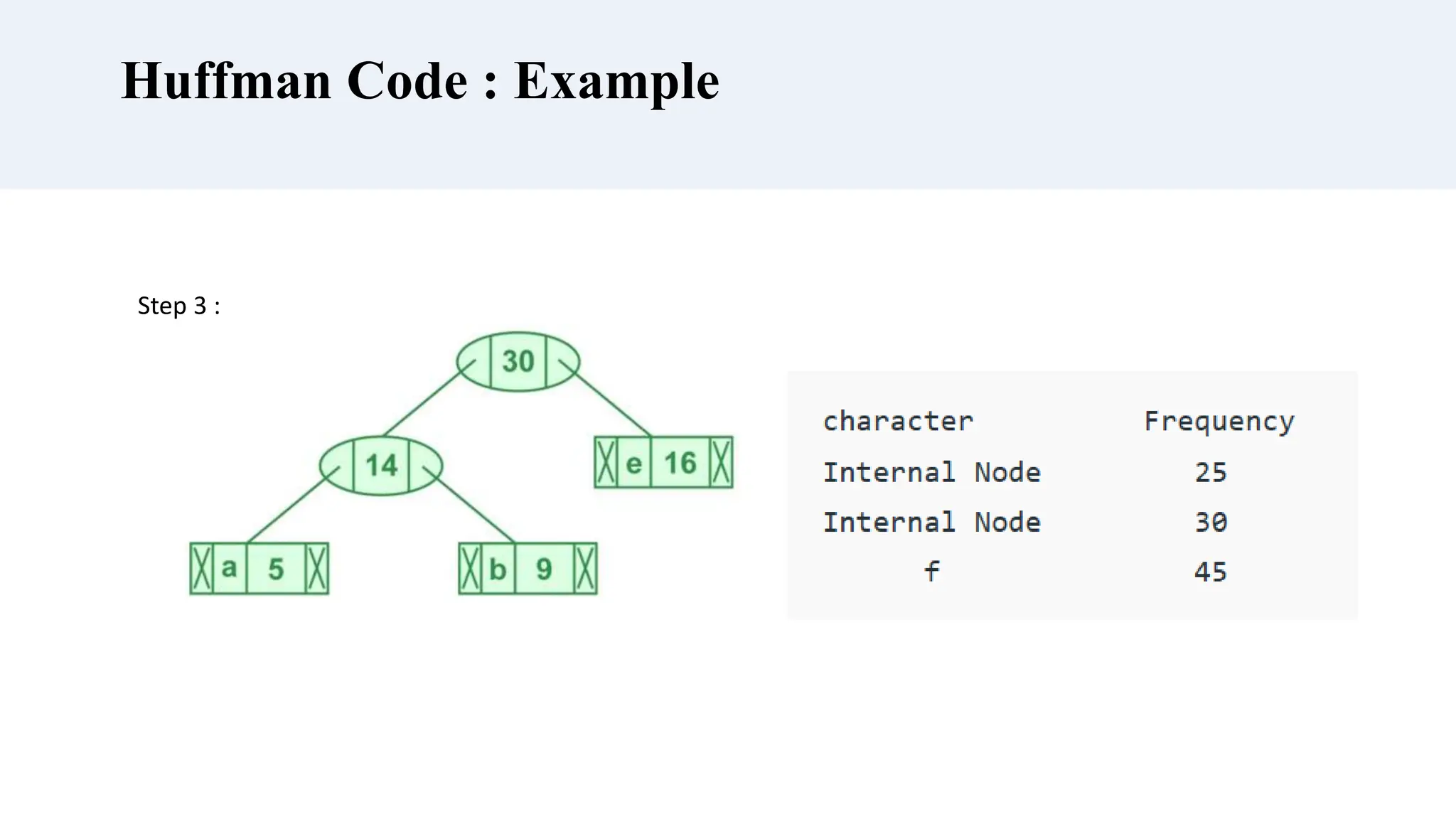
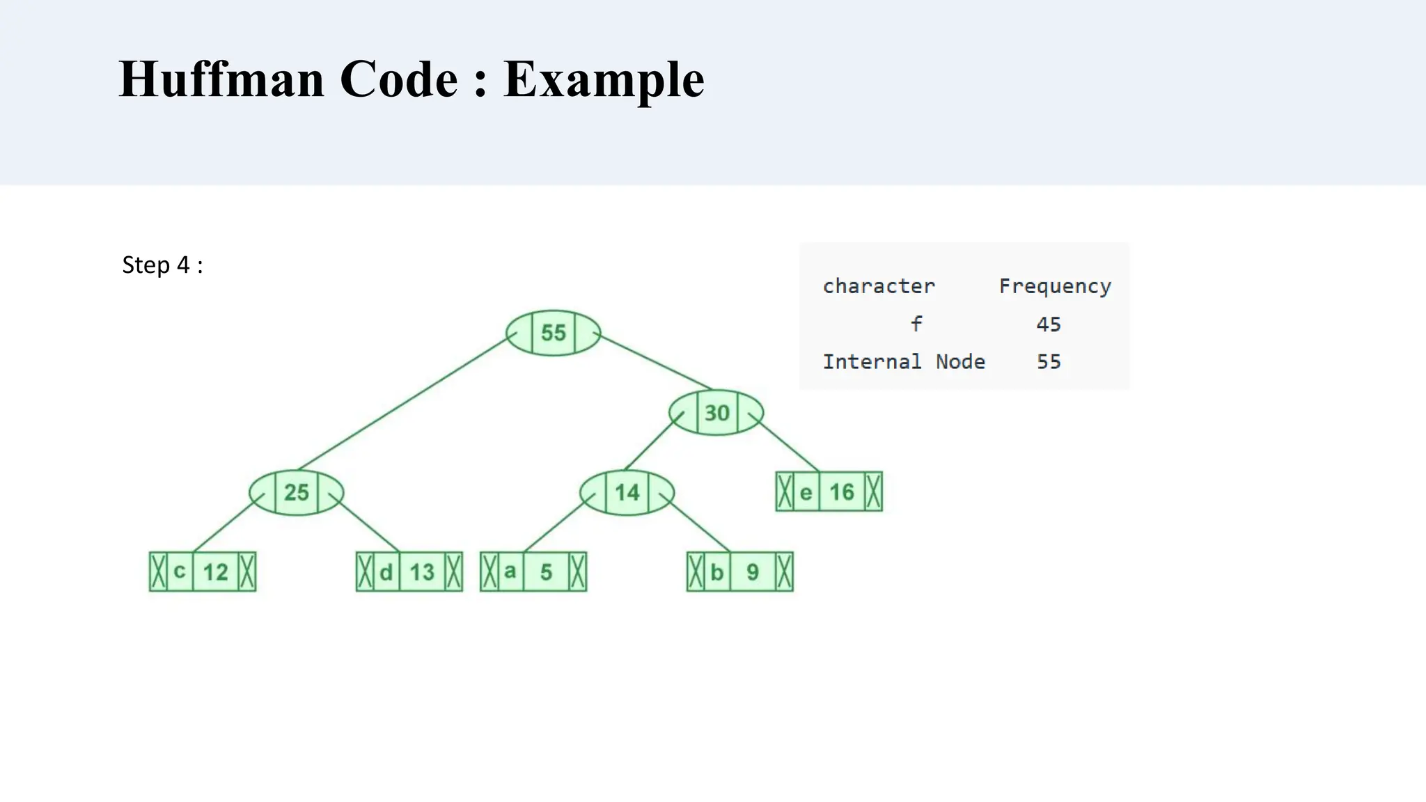
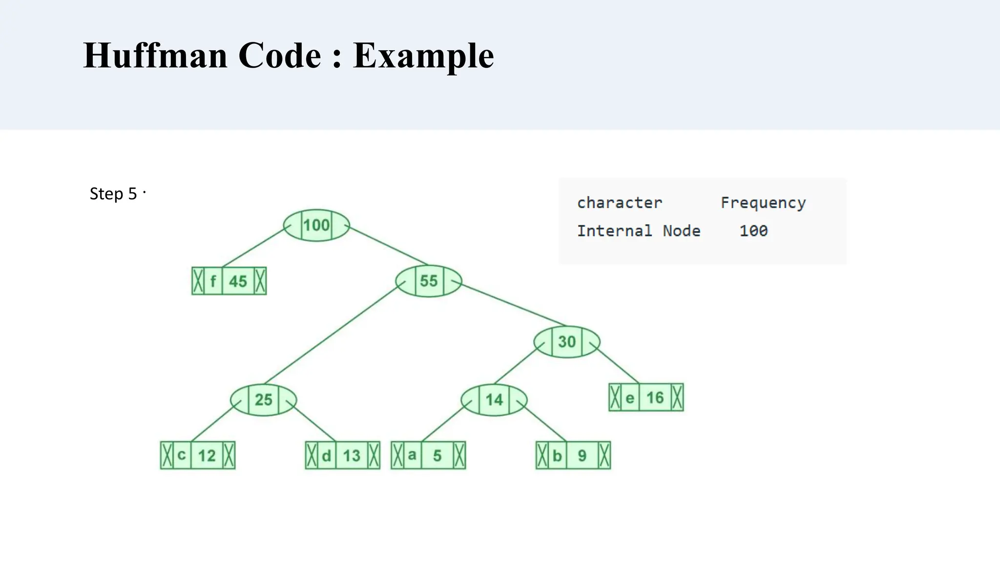
![Huffman Code : Algorithm
There are mainly two major parts in Huffman
Coding
• Build a Huffman Tree from input characters.
• Traverse the Huffman Tree and assign codes
to characters.
Algorithm Huffman (c)
{
n= |c|
Q = c
for i<-1 to n-1
do
{
temp <- get node ()
left (temp] Get_min (Q) right [temp] Get Min (Q)
a = left [templ b = right [temp]
F [temp] = f[a] + [b]
insert (Q, temp)
}
return Get_min (0)
}](https://image.slidesharecdn.com/daa-unit2-240325042900-457be414/75/Data-analysis-and-algorithms-UNIT-2-pptx-17-2048.jpg)


![[DSC Europe 25] Bassam Maharmeh - Artificial Intelligence: Opportunities and ...](https://cdn.slidesharecdn.com/ss_thumbnails/thhfmr2fqpawzj7hsjpg-5-251211083048-2c23204f-thumbnail.jpg?width=640&height=640&fit=bounds)


![[DSC Europe 25] Jovan Bogicevic - Legacy to AI-Driven Defense: Transforming D...](https://cdn.slidesharecdn.com/ss_thumbnails/rsarluadt563hntyfc8q-3-251211083849-3e7bc4c0-thumbnail.jpg?width=640&height=640&fit=bounds)


![[DSC Europe 25] Dobrica Cosic - Savings by the Second: How Dynamic Pricing an...](https://cdn.slidesharecdn.com/ss_thumbnails/znp09f3smtqz3w2sq6wn-1-dobrica-cosic-savings-by-the-second-how-dynamic-pricing-and-smart-data-are-bu-251208151905-26e6f41e-thumbnail.jpg?width=640&height=640&fit=bounds)


![[DSC Europe 25] Branko Urosevic -Rethinking Financial Talent: Integrating Cod...](https://cdn.slidesharecdn.com/ss_thumbnails/8jjrus8ttko6qj64f58f-3-251212103250-642c6374-thumbnail.jpg?width=640&height=640&fit=bounds)
![[DSC Europe 25] Dunja Adzic Jovanovic - AI and Cybersecurity: Defending Data ...](https://cdn.slidesharecdn.com/ss_thumbnails/o1zylpbhrtwnixxq2xj8-7-251211083048-185086f6-thumbnail.jpg?width=640&height=640&fit=bounds)
![[DSC Europe 25] Vladimir Jelic - The AI-Driven Security Shift From Reactive D...](https://cdn.slidesharecdn.com/ss_thumbnails/6g5gj25mtjwayniqem1t-6-251209104645-7a5a5fc6-thumbnail.jpg?width=640&height=640&fit=bounds)
![[DSC Europe 25] Milan Sekuloski - Data, Defence, and Development: Cybersecuri...](https://cdn.slidesharecdn.com/ss_thumbnails/dfrkwwx4qly6atqpbl4z-4-251209104645-c3d4b0ca-thumbnail.jpg?width=640&height=640&fit=bounds)