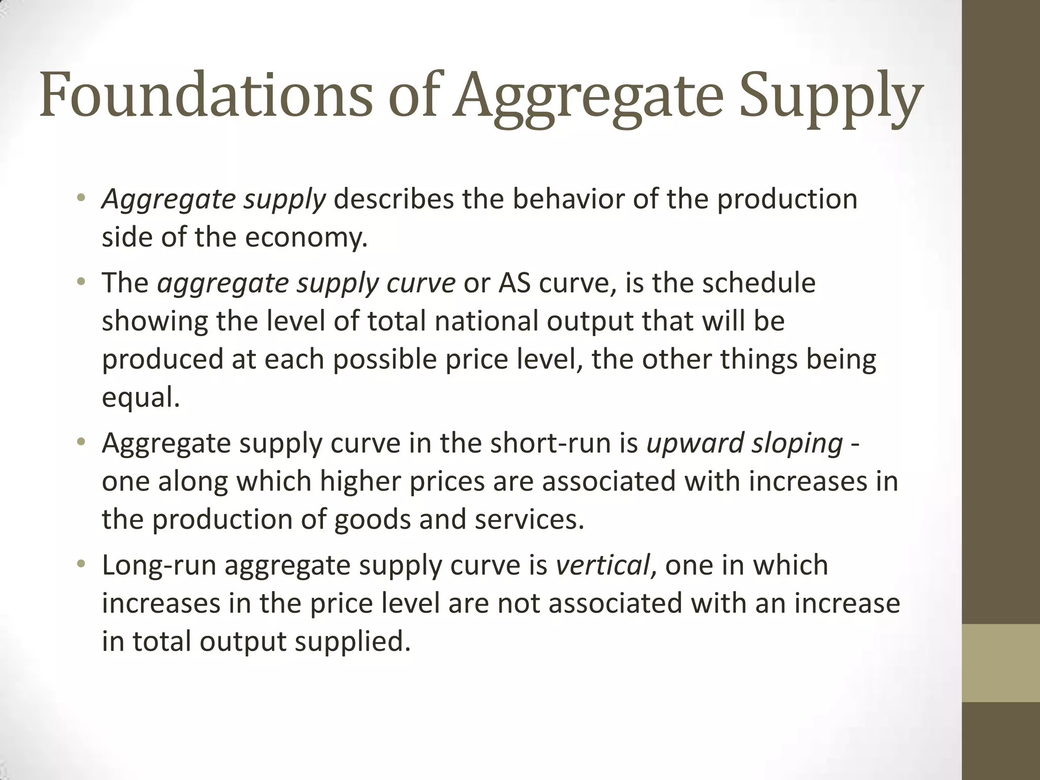
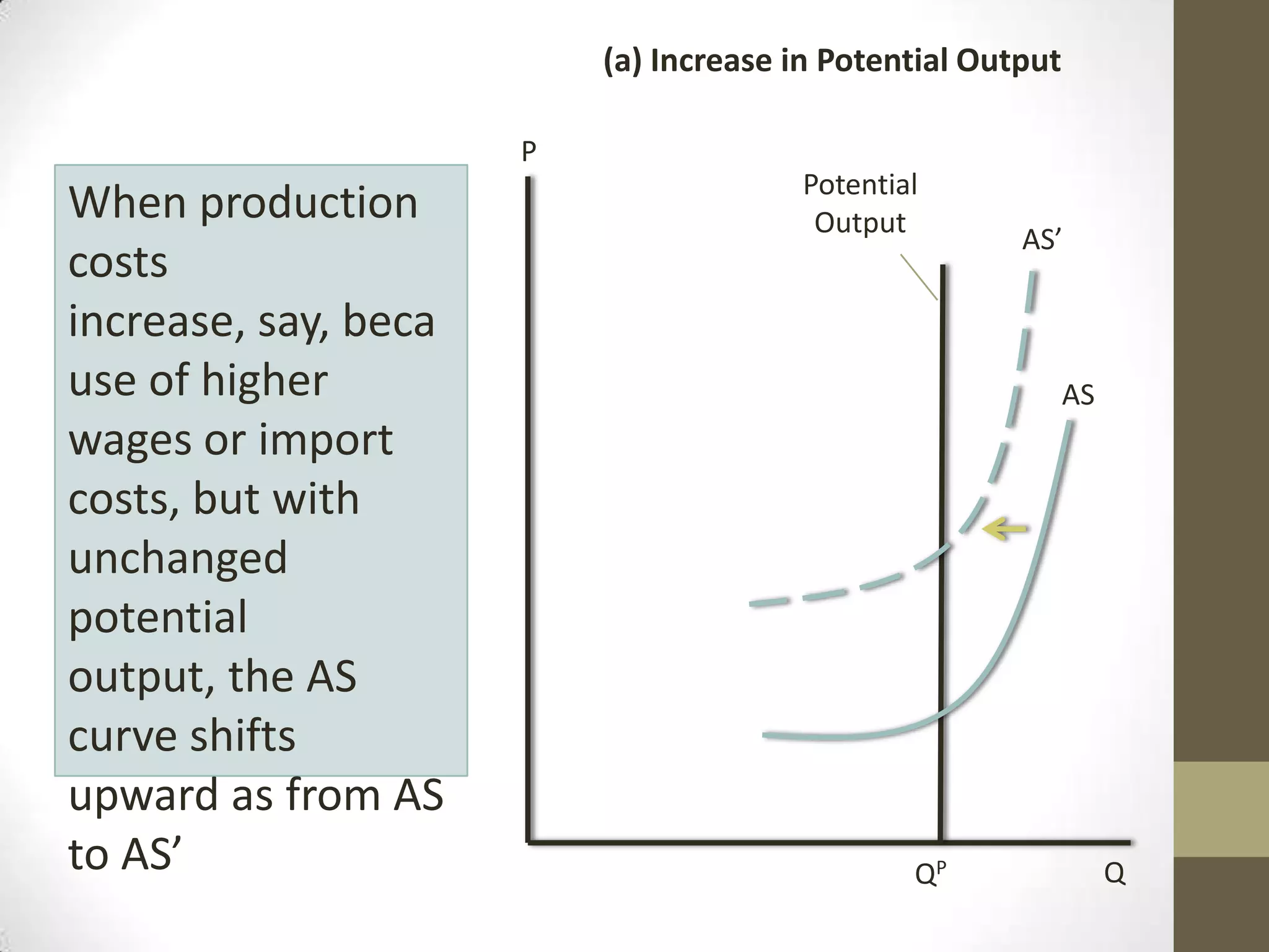
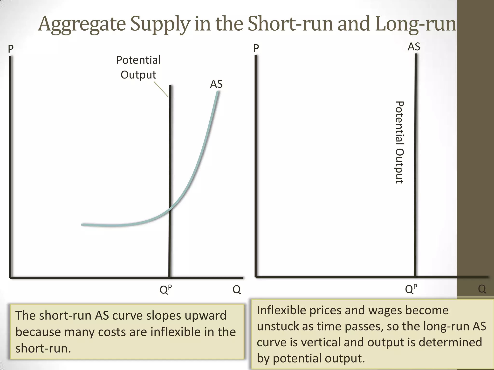
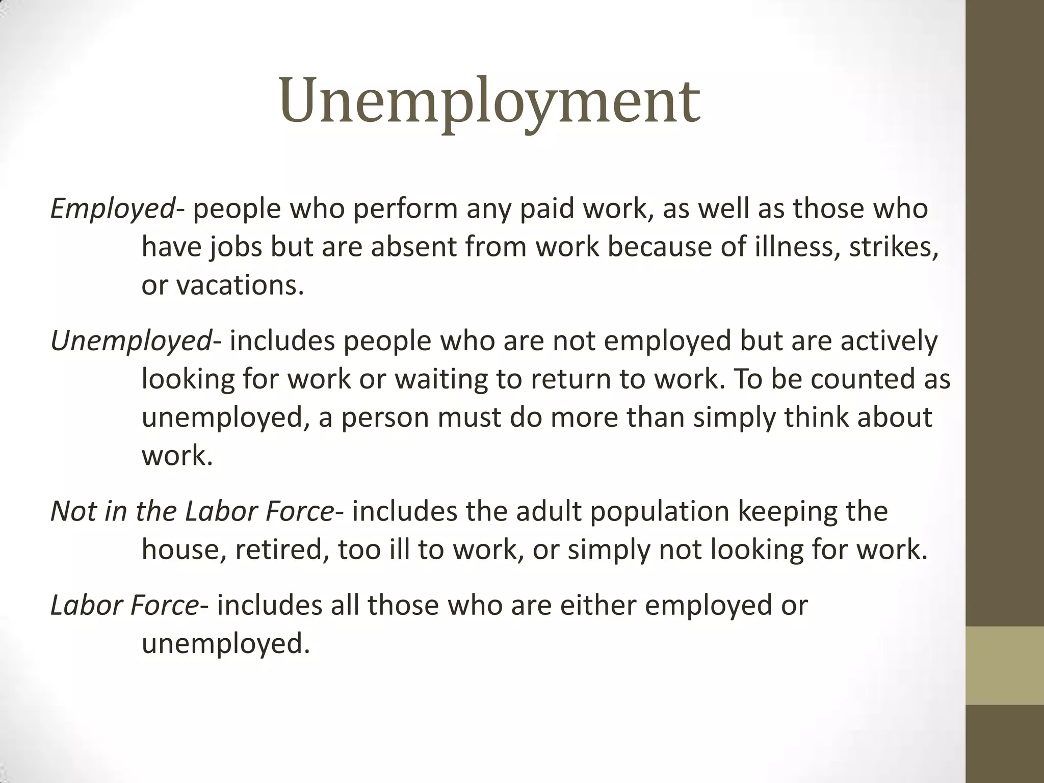
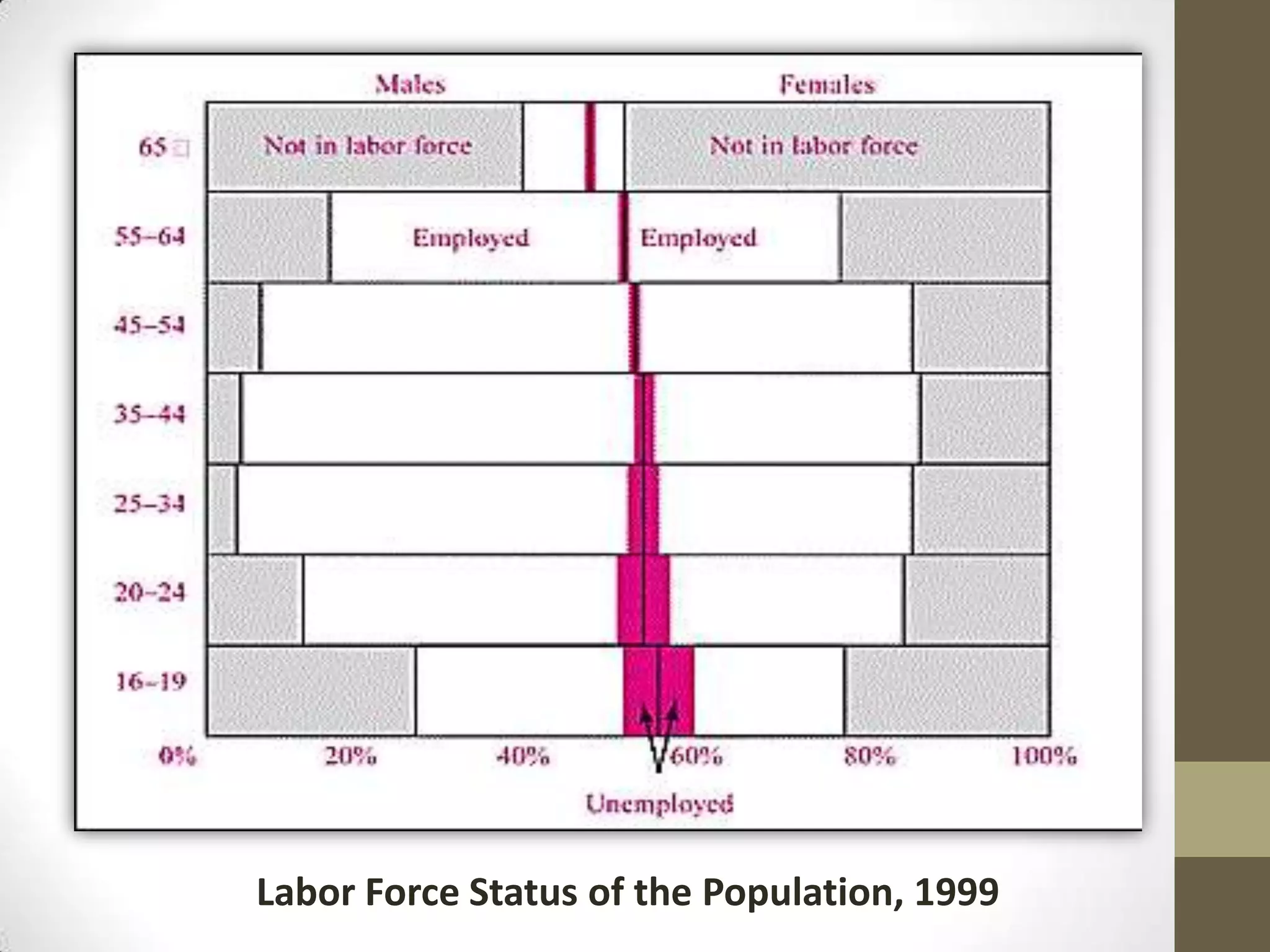
The document discusses aggregate supply and unemployment. It defines aggregate supply as the total output produced at different price levels. The aggregate supply curve is upward sloping in the short-run but vertical in the long-run. Unemployment decreases potential output and shifts the aggregate supply curve left. High unemployment represents wasted resources and causes social problems. There are different types of unemployment including frictional, structural, and cyclical unemployment.

1. Unemployment and the
Foundations of
Aggregate Supply

2. Foundations of Aggregate Supply
• Aggregate supply describes the behavior of the production
side of the economy.
• The aggregate supply curve or AS curve, is the schedule
showing the level of total national output that will be
produced at each possible price level, the other things being
equal.
• Aggregate supply curve in the short-run is upward sloping -
one along which higher prices are associated with increases in
the production of goods and services.
• Long-run aggregate supply curve is vertical, one in which
increases in the price level are not associated with an increase
in total output supplied.

3. Determinants of Aggregate Supply
• Aggregate supply depends fundamentally upon
two distinct set of forces: potential output and
input costs.
• Potential output is the highest sustainable level
of national output.
• Input cost is the cost incurred in the production
of goods and services.

4. Variable Impact on Aggregate Supply
Potential Output
Inputs Supplies of capital, labor and land are the important inputs.
Potential outputs comes when unemployment of labor and
other resources is at non-inflationary levels. Growth of
inputs increases potential output and aggregate supply.
Technology and Innovation, technological improvement, and increased
Efficiency efficiency increase the level of potential output and raise
aggregate supply.
Production Costs
Wages Lower wages lead to lower production costs; lower costs
mean that quantity supplied will be higher at every price
level for a given potential output.
Import Prices A decline in foreign prices or an appreciation in the
exchange rate reduces import prices. This leads to lower
production costs and raises aggregate supply.
Other input costs Lower oil prices or less burdensome environmental
regulation lowers production costs and thereby raises
aggregate supply.

5. (a) Increase in Potential Output
Potential
P Output
AS AS’
Growth in
potential output
with unchanged
production costs
shifts the AS
curve rightward
from AS to AS’.
QP QP ’ Q

6. (a) Increase in Potential Output
P
Potential
When production Output
AS’
costs
increase, say, beca
use of higher AS
wages or import
costs, but with
unchanged
potential
output, the AS
curve shifts
upward as from AS
to AS’ QP Q

7. Aggregate Supply in the Short-run and Long-run
P P AS
Potential
Output
AS
Potential Output
QP Q QP Q
The short-run AS curve slopes upward Inflexible prices and wages become
because many costs are inflexible in the unstuck as time passes, so the long-run AS
short-run. curve is vertical and output is determined
by potential output.

8. Unemployment
Employed- people who perform any paid work, as well as those who
have jobs but are absent from work because of illness, strikes,
or vacations.
Unemployed- includes people who are not employed but are actively
looking for work or waiting to return to work. To be counted as
unemployed, a person must do more than simply think about
work.
Not in the Labor Force- includes the adult population keeping the
house, retired, too ill to work, or simply not looking for work.
Labor Force- includes all those who are either employed or
unemployed.

9. Labor Force Status of the Population, 1999

10. Impact of Unemployment
• High unemployment is both an economic and social
problem. Unemployment is an economic problem
because it represents waste of a valuable resource.
• It is a major social problem because it causes
enormous suffering as the unemployed workers
struggle with reduced incomes.

11. Lost Output
Average GDP loss As percentage of
Unemployment ($, billion, 1999 GDP during the
rate (%) prices) period
Great Depression (1930-1939) 18.2 2,420 27.6
Oil and Inflation crises (1975-1984) 7.7 1,480 3.0
New Economy period (1985-1999) 5.7 240 0.3
Economic Costs from Periods of High Unemployment
The two major periods of high unemployment occurred during the
Great Depression and during the oil shocks and high inflation. The lost
output is calculated as the cumulative difference between potential
GDP and actual GDP.

12. Okun’s Law
• For every 2 percent that GDP falls relative to potential GDP, the
unemployment rate rises about 1 percentage point.
• One important consequence of Okun’s law is that actual GDP must
grow as rapidly as potential GDP just to keep the unemployment
rate from rising.
Okun’s Law
Illustrated,
(1955-1999)

13. Economic Interpretation of Unemployment
• Three Kinds of Unemployment
- Frictional Unemployment- arises because of the incessant
movement of people between regions and jobs or through
different stages of the life cycle.
- Structural Unemployment- signifies a mismatch between
the supply and demand for workers.
- Cyclical Unemployment- exists when the overall demand for
labor is low.

14. Voluntary and Involuntary Unemployment
Wages move to W* to clear S
W
the labor market. All D
unemployment is voluntary.
At the competitive, market-
clearing equilibrium, firms
willingly hire all qualified
workers who desire to work
at the market wage.
The number of unemployed
is the line from A to E.
Some members of the labor
Employed E
force would like to work, W* F
but only at a higher wage A
Voluntary
rate and these are the S Unemployment D
voluntary unemployed L
workers (segment EF). L*
Flexible wages

15. S
W
D
The graph shows what
happens if wages do
not adjust to clear the
labor market. At the
too high wage at W**, Involuntary
Employed Unemployment
JH workers are W** G
J H
employed, but HG
workers are E
W*
involuntarily
unemployed. S D
L
L*
Inflexible wages

16. Labor Market Issues
• Who are the unemployed
• Duration of unemployment
• Source of Joblessness
• Unemployment by Age

17. Unemployment rate of different Distribution of total unemployment
groups across different groups
(% of labor force) (%of total unemployed.)
Labor Market Group Recession Boom Recession Boom
(1982) (March 2000) (1982) (March 2000)
By age:
16-19 23.2 13.3 18.5 20.2
20 and older 8.6 3.3 81.5 80.0
By Race:
White 8.6 3.6 77.2 77.6
Black and other 17.3 7.3 22.8 22.4
By Sex (Adults only):
Male 8.8 3.8 58.5 50.5
Female 8.3 4.3 41.5 49.5
All Workers 9.7 4.1 100.0 100.0
Unemployment by Demographic Group
This table shows how unemployment varies across different demographic
groups in boom and recession years. The first set of figures shows the unemployment
rate for each group in 1982 and during the boom period of 2000. the last two columns
show the percent of the total pool of unemployed that is in each group.

18. 45
40
35
30
25
20
15
10
5
0
<5 10-14 15-26 27-51 52+
Duration of Unemployment, 1999 (weeks)
The duration figures show the distribution of length of unemployment. In the
full-employment year 1999, only 14% were unemployed for less than 5
weeks. In recessions, duration of unemployment increases.

19. Recession
Unemployment by
Reason
(percent of the labor
force that is unemployed
Job Loser 5.7 for different reasons)
Boom
Reentrant 2.2 Job Loser
1.9
New Entrant 1.1 1.4 Reentrant
0.3 New Entrant
Job Leaver 0.8 0.6 Job Leaver
1982 1999
Distribution of Unemployment by Reasons, 1982 and 1999
very few were unemployed in 1999 because they left their jobs, and
almost 2% were new entrants into the labor force or reentrants. The major change
in unemployment from boom to recession, however, Is found in the number of job
losers.

20. Unemployment rate
(% of labor force)
Age White Black
16-17 14.5 31.0
18-19 10.2 26.2
20-24 6.3 14.6
25-34 3.3 7.6
35-44 2.7 5.3
45-54 2.4 4.0
55-64 2.5 3.9
65 and older 2.9 5.0
Unemployment Rates at Different Ages
as workers search for jobs and gain training, they settle on a
particular occupation; they tend to stay in the labor force and they find a
preferred employer. As a result, the unemployment rates of older people fall
to a fraction of those of teenagers.