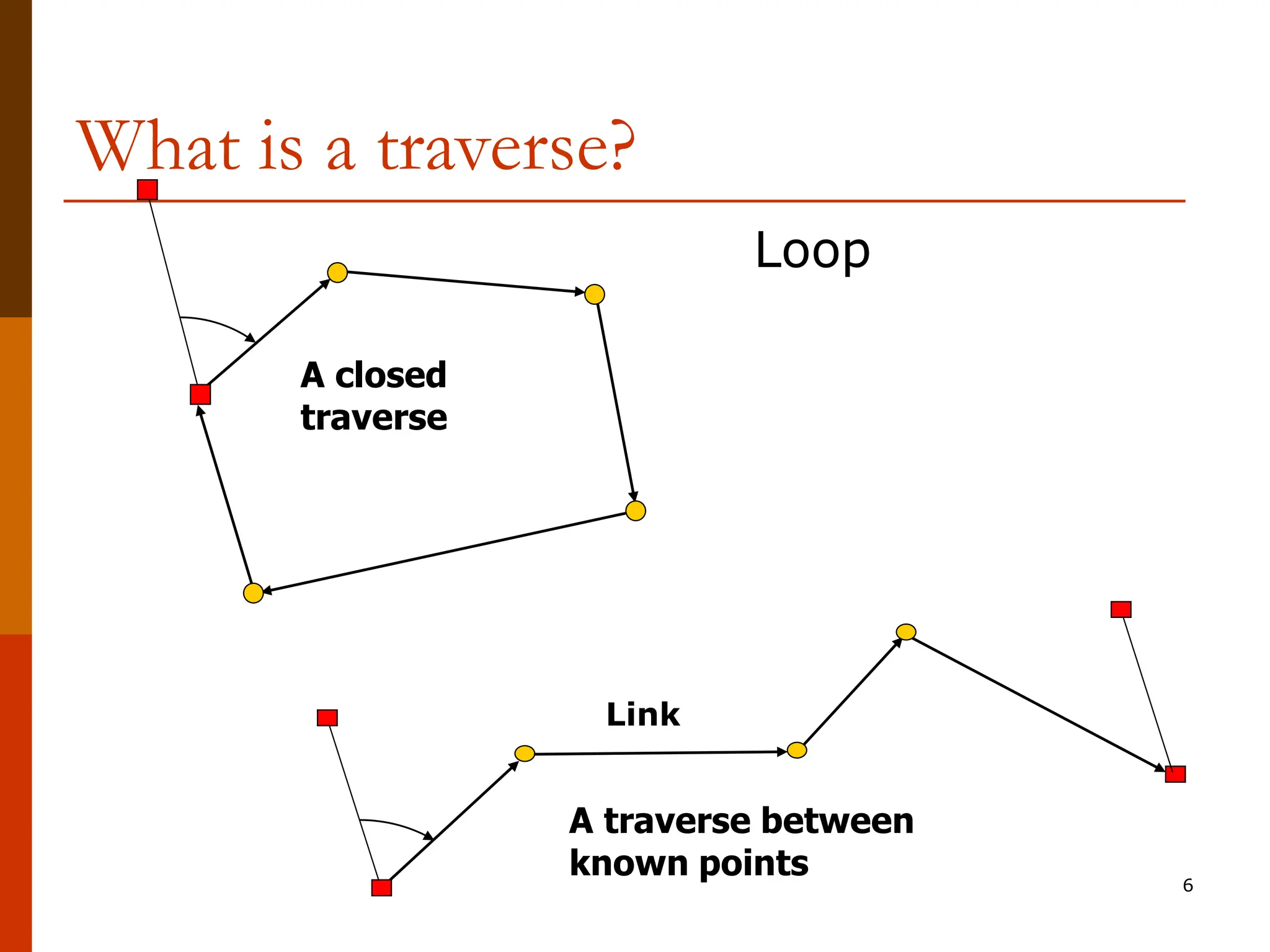
The document discusses the concept of traversing in civil engineering, highlighting the two types of traverses: closed and open. It describes the procedures for performing traverse computations, establishing coordinates, and managing angular and linear misclosure errors. Additionally, it explains methods for adjusting data to ensure mathematical closure in traverse surveys while maintaining accuracy.

1. Traverse Computations
In Civil Works

2. 2
Traverse
 A traverse is a series of consecutive lines
whose ends have been marked in the field,
and whose lengths and directions have
been determined from measurements
► Used to locate topographic details for
the preparation of plans
► To lay out (setting-out) or locate
engineering works

3. Two types
 Close
 Open
Main applications of traversing
 Establishing coordinates for new points
(E,N)new
(E,N)new
(E,N)known
(E,N)known
(E,N)known
(E,N)known

4. 4
Closed traverse
 Closed traverse can be link or polygon
 Polygon (loop)
 The lines returns to the starting point, thus
forming a closed figure
 Geometrically and mathematically closed
 Link
 Begins and ends at points whose positions have
been previously determined
 Geometrically open, mathematically closed

5. 5
Open traverse
 Series of measured lines and angles that do
not return to the starting point or close upon
a previously determined point.
 Geometrically and mathematically open
 Lack of geometrical closure means no
geometrical verification of actual positions of
traverse stations
 No means of checking for observational
errors and mistakes
 Should be avoided

6. 6
What is a traverse?
A closed
traverse
A traverse between
known points
Loop
Link

7. 7
Traverse computation
 Traverse computations are concerned with
deriving co-ordinates for the new points
that were measured, along with some
quantifiable measure for the accuracy of
these positions.
 The co-ordinate system most commonly
used is a grid based rectangular orthogonal
system of eastings (X) and northings (Y).
 Traverse computations are cumulative in
nature, starting from a fixed point or known
line, and all of the other directions or
positions determined from this reference.

8. 8
Choosing location of traverse stations
1. Minimize # of stations (each line of sight: as
long as possible)
2. Ensure: adjacent stations always inter-visible
3. Avoid acute traverse angles
4. Stable & safe ground conditions for instrument
5. Marked with paint or/and nail; to survive
subsequent traffic, construction, weather
conditions, etc.

9. 9
6. Include existing stations / reference objects
for checking with known values
7. Traverse must not cross itself
8. Network formed by stations (if any): as
simple as possible
9. Do the above without sacrificing accuracy or
omitting important details
Choosing location of traverse stations

10. Datum check
 Check if the opening and closing control
points are in-situ
 Measure distance between and check the
direction by compass/or a theodolite
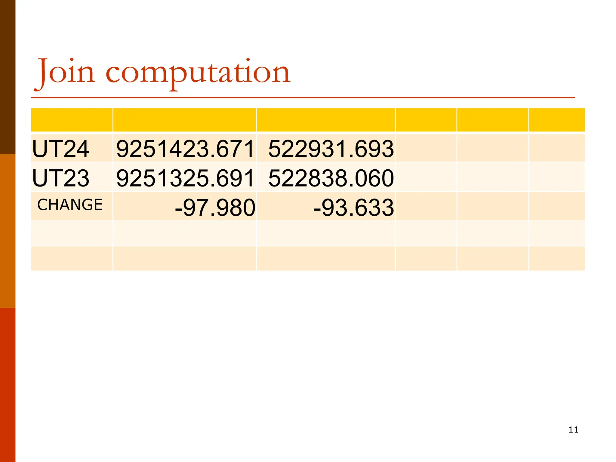
 Compute the distance and bearings by
join computation
 Compare the results [should be within
limits]
10

11. Join computation
UT24 9251423.671 522931.693
UT23 9251325.691 522838.060
CHANGE -97.980 -93.633
11

12. 12
Traverse Computation
1)Calculation of starting and closing bearings;
2)Calculation of angular misclosure by
comparing the sum of the observed bearings
with the closing bearings.
3)If angular misclosure is acceptable,
distribute it throughout the traverse in equal
amounts to each angle.
4)Reduction of slope distance to horizontal
distance;

13. 13
Traverse Computation (con’t)
5)Calculation of the changes in coordinates
(N, E) of each traverse line.
6)Assessing the coordinate misclosure.
7)Balancing the traverse by distributing the
coordinate misclosure throughout the
traverse lines.
8)Computation of the final coordinates of each
point relative to the starting station, using
the balanced values of N, E per line.

14. 14
Angular misclosure
 The numerical diff. between the existing
bearing and the measured one is called
the angular misclosure.
 There is usually a permissible limit for
this misclosure, depending upon the
accuracy requirements and
specifications of the survey.

15. Angular misclosure
 A typical computation for the allowable
misclosure  is given by = kn
 where n is the number of angles
measured and k is a fraction based on
the least division of the theodolite
scale.
 E.g, if k is 1”, for a traverse with 10
measured angles, the allowable
misclosure is 3.1623”.
15

16. Angular misclosure
 For a closed link traverse, the check is
given by
 A1 +(angles) – A2 = (n – 1) 180
 where A1 is the initial or starting
bearing, A2 is the closing or final
bearing, and n is the number of
angles measured.
16

17. 17
Angular misclosure
 Once the traverse angles are within
allowable range, the remaining misclosure
is distributed amongst the angles.
 This process is called balancing the angles
as follows
 Average adjustment
 Misclosure is divided by number of angles and
correction inserted into all of the angles.
 Most common technique

18. 18
Angular misclosure
 Arbitrary adjustment
 if misclosure is small, then it may be inserted
into any angle arbitrarily (usually one that may
be suspect).
 If no angle suspect, then it can be inserted into
more than one angle.
 Adjustment based on measuring conditions
 If a line has particular obstruction that may have
affected observations, misclosure may be divided
and inserted into the two angles affected.

19. 19
Traversing - Computations
 Errors in angular measurement are not
related to the size of the angle.
 Once the angles have been balanced, they
can be used to compute the bearings of the
lines in the traverse.
 Starting from the bearing of the original fixed
control line, the internal or clockwise
measured angles are used to compute the
forward azimuths of the new lines.
 The bearing of this line is then used to
compute the bearing of the next line and so
on

20. 20
Misclosure and adjustment
 For closed traverses, co-ordinates of the final
ending station are known, this provides a
mathematical check.
 If the final computed E and N are compared
to the known E and N for the closing station,
then co-ordinate misclosures can be
determined.
 The E misclosure E is given by
 dE = final computed E – final known E
 similarly, the N misclosure N is given by
 dN = final computed N – final known N

21. 21
Linear Misclosure of Traverse
2 2
dE dN
  
dE = error in easting of last station (= observed - known)
dN = error in northing of last station (= observed - known)
Fractional accuracy: f
L



Order Max  Max f Typical survey task
First 1 in 25000 Control or monitoring surveys
Second 1 in 10000 Engineering Surveying;
Setting out surveys
Third 1 in 5000
2 n
10 n
30 n

22. 22
Example: Traverse Computation (con’t)
Another options
For each leg, calculate N [Dist * cos(Brg)] & E
[Dist * sin(Brg)].
Compute Sum N and Sum E.
Compare results with diff. between start and end
coords.
The difference is dE and dN

23. 23
Linear Misclosure
•These discrepancies represent the difference on the
ground between the position of the point computed from
the observations and the known position of the point.
•The E and N misclosures are combined to give the
linear misclosure of the traverse, where
linear misclosure = (E2 + N2)
E
N

24. 24
Traversing – Precision
 By itself the linear misclosure only gives a
measure of how far the computed position
is from the actual position (accuracy of the
traverse measurements).
 Another parameter that is used to provide
an indication of the relative accuracy of
the traverse is the proportional linear
misclosure.

25. 25
Traversing - Computations
 If a misclosure exists, then the figure
computed is not mathematically closed.
 This can be clearly illustrated with a closed
loop traverse.
 The co-ordinates of a traverse are
therefore adjusted for the purpose of
providing a mathematically closed figure
while at the same time yielding the best
estimates for the horizontal positions for
all of the traverse stations.

26. 26
 Discrepancies between eastings and
northings must be adjusted before
calculating the final coordinates.
Adjustment methods:
 Compass Rule
 Least Squares Adjustment
 Bowditch Rule
 Bowditch Rule is most commonly used.
Adjustment of Traverse

27. 27
 devised by Nathaniel Bowditch in 1807.
Adjustment by Bowditch Rule
Ei, Ni = Coordinate corrections
dE, dN = Coordinate Misclosure (constant)
Li = Sum of the lengths of the traverse (constant)
Li = Horizontal length of the ith traverse leg.
i
n
i
i
i L
L
dE
E 


1
 i
n
i
i
i L
L
dN
N 


1


28. 28
Adjustments - Arbitrary
 The arbitrary method is based upon the
surveyor’s individual judgement
considering the measurement conditions.
 The Least Squares method is a rigorous
technique that is founded upon
probabilistic theory.
 It requires an over-determined solution
(redundant measurements) to compute
the best estimated position for each of the
traverse stations.

29. 29
Adjustments – Transit Rule
 The transit rule applies adjustments
proportional to the size of the easting or
northing component between two stations
and the sum of the easting and northing
differences.

30. 30
Example: Closed Traverse Computation
Measurements of traverse ABCDE are given
in Table 1. Given that the co-ordinates of A
are 782.820mE, 460.901mN; and co-
ordinates of E are 740.270mE, 84.679mN.
The WCB of XA is 123-17-08 and WCB of EY
is 282-03-00.

31. 31
Example: Traverse Computation (con’t)
a)Determine the angular, easting, northing and
linear misclosure of the traverse.
b)Calculate and tabulate the adjusted co-
ordinates for B, C and D using Bowditch Rule.
Station Clockwise angle Length (m)
A 260-31-18
B 123-50-42 129.352
C 233-00-06 81.700
D 158-22-48 101.112
E 283-00-18 94.273

32. 32
Example: Traverse Computation (con’t)
1)There is no need to calculate the starting
and ending bearings as they are given.
2)Calculate the angular misclosure and
angular correction using:
F’ = I + sum of angles - (n x 180)

33. 33
Example: Traverse Computation (con’t)
F’ = I + sum of angles - (n x 180)
sum of angles
= (260-31-18) + (123-50-42) + (233-00-06) +
(158-22-48) + (283-00-18) = (1058-45-12)
I = 123-17-08; (n x 180) = 900
F’ = (123-17-08) + (1058-45-12) - 900 = 282-
02-20
angular misc. = (282-02-20) - (282-03-00) = -
40”
 As there are five angles, each will be added
by the following factor of (40”/5) = 8”.

34. 34
Example: Closed Traverse
Computation (con’t)
Angular correction:
AX 303-17-08
A 260-31-18
(+8”)
563-48-34
360-00-00
A to B 203-48-34
180-00-00
B to A 23-48-34
 B 123-50-42(+8”)
B to C 147-39-24
180-00-00
C to B 327-39-24
 C 233-00-
06(+8”)
560-39-38
360-00-00
C to D 200-39-38

35. 35
Example: Closed Traverse
Computation (con’t)
C to D 200-39-38
180-00-00
D to C 20-39-38
 D 158-22-
48(+8”)
D to E 179-02-34
180-00-00
E to D 359-02-34
 E 283-00-
18(+8”)
642-03-00
360-00-00
E to Y282-03-00
(checks)

36. 36
Example: Closed Traverse
Computation (con’t)
Set up table and fill in bearings, distances,
starting and ending bearings. Calculate
the total traversed distance.
Sta. Brg Dist N E N E
A 460.901 782.820
B 203-48-34 129.352
C 147-39-24 81.700
D 200-39-38 101.112
E 179-02-34 94.273 84.679 740.270
406.437 84.679 740.270
-460.901 -782.820
-376.222 -42.550

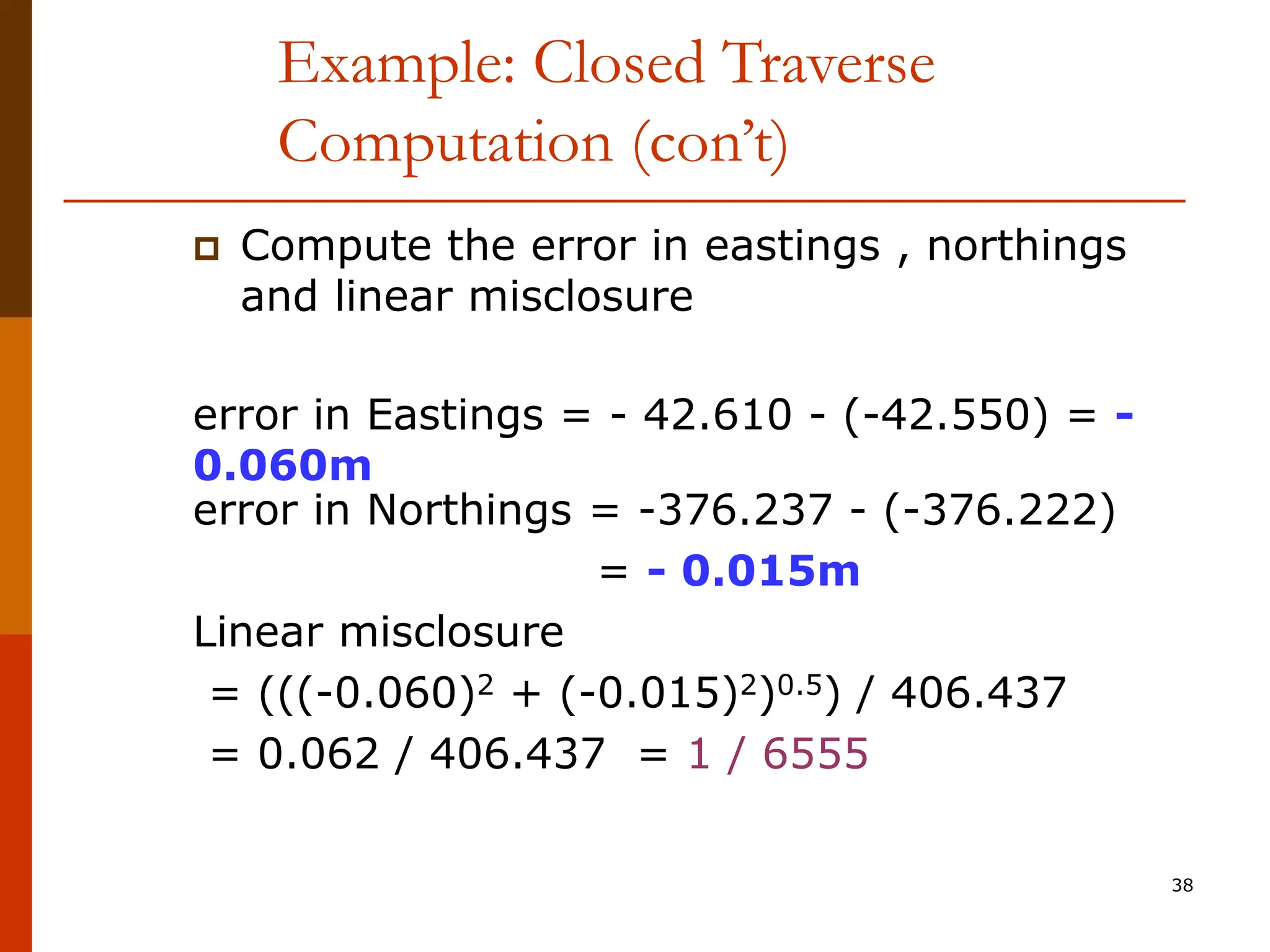
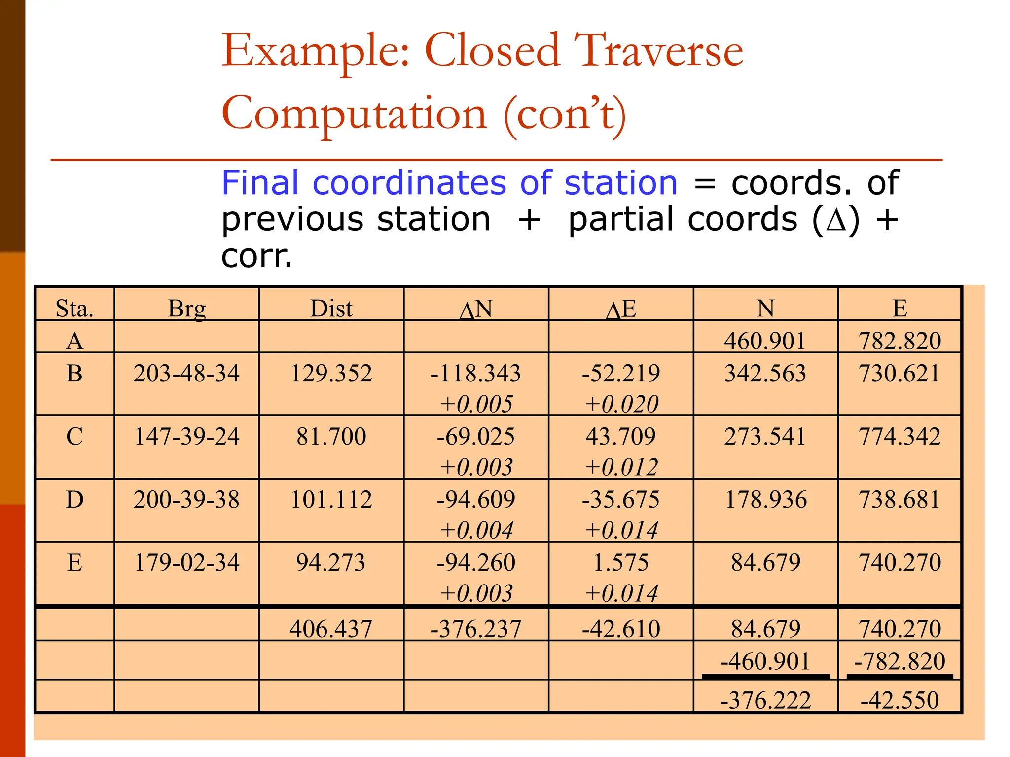
37. 37
Example: Closed Traverse
Computation (con’t)
For each leg, calculate N [Dist *
cos(Brg)] & E [Dist * sin(Brg)]. Sum N
and E. Compare results with diff.
between start and end coords.
Sta. Brg Dist N E N E
A 460.901 782.820
B 203-48-34 129.352 -118.343 -52.219
C 147-39-24 81.700 -69.025 43.709
D 200-39-38 101.112 -94.609 -35.675
E 179-02-34 94.273 -94.260 1.575
406.437 -376.237 -42.610 84.679 740.270
-460.901 -782.820
-376.222 -42.550

38. 38
Example: Closed Traverse
Computation (con’t)
 Compute the error in eastings , northings
and linear misclosure
error in Eastings = - 42.610 - (-42.550) = -
0.060m
error in Northings = -376.237 - (-376.222)
= - 0.015m
Linear misclosure
= (((-0.060)2 + (-0.015)2)0.5) / 406.437
= 0.062 / 406.437 = 1 / 6555

39. 39
Example: Closed Traverse
Computation (con’t)
Using Bowditch Rule, calculate correction
for each N & E. ((partial dist./total
dist.) * (error in N or E)
Sta. Brg Dist N E N E
A 460.901 782.820
B 203-48-34 129.352 -118.343
+0.005
-52.219
+0.020
C 147-39-24 81.700 -69.025
+0.003
43.709
+0.012
D 200-39-38 101.112 -94.609
+0.004
-35.675
+0.014
E 179-02-34 94.273 -94.260
+0.003
1.575
+0.014
406.437 -376.237 -42.610 84.679 740.270
-460.901 -782.820
-376.222 -42.550

40. 40
Example: Closed Traverse
Computation (con’t)
Final coordinates of station = coords. of
previous station + partial coords () +
corr.
Sta. Brg Dist N E N E
A 460.901 782.820
B 203-48-34 129.352 -118.343
+0.005
-52.219
+0.020
342.563 730.621
C 147-39-24 81.700 -69.025
+0.003
43.709
+0.012
273.541 774.342
D 200-39-38 101.112 -94.609
+0.004
-35.675
+0.014
178.936 738.681
E 179-02-34 94.273 -94.260
+0.003
1.575
+0.014
84.679 740.270
406.437 -376.237 -42.610 84.679 740.270
-460.901 -782.820
-376.222 -42.550

41. ERROR PROPAGATION IN
TRAVERSE SURVEYS
41

42.  Even though the specifications for a project may allow lower accuracies,
the presence of blunders in observations is never acceptable.
 Thus, an important question for every surveyor is: How can I tell when
blunders are present in the data?
 Generally, observations in horizontal surveys (e.g., traverses) are
independent. That is, the measurement of a distance observation is
independent of the azimuth observation .But the latitude and departure
of a line, which are computed from the distance and azimuth
observations, are not independent.
42

43.  The following figure shows the effects of errors in distance and azimuth
observations on the computed latitude and departure. In the figure it can be
seen that there is correlation between the latitude and departure; that is, if
either distance or azimuth observation changes, it causes changes in both
latitude and departure.
43

44. DERIVATION OF ESTIMATED ERROR IN LATITUDE
AND DEPARTURE
44

45.  The estimated errors in these values are solved using matrix Equation as
45

46.  propagation of observational errors through traverse computations has been
discussed.
 Error propagation is a powerful tool for the surveyor, enabling an answer to
be obtained for the question: What is an acceptable traverse misclosure?
This is an example of surveying engineering.
 Surveyors are constantly designing measurement systems and checking
their results against personal or legal standards. The subjects of error
propagation and detection of measurement blunders are discussed further
in later chapters.
46