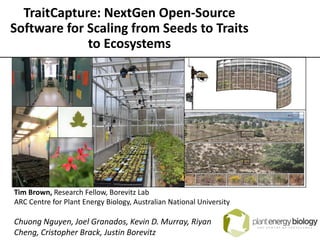
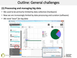
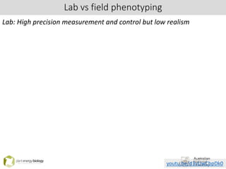
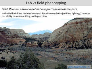
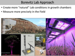
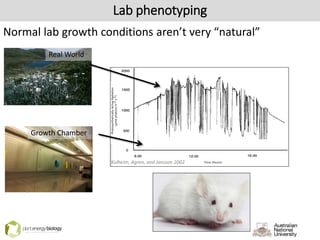
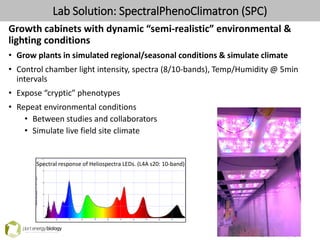
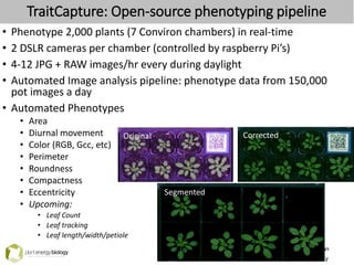
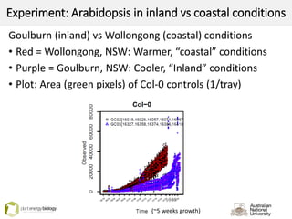
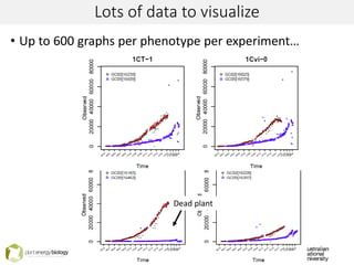
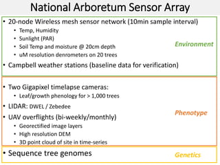
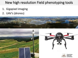
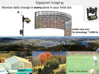
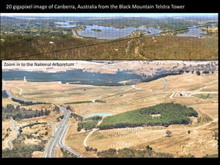
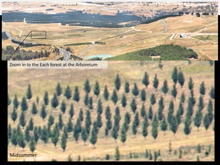
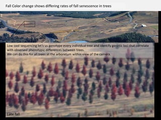
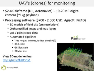
TraitCapture: NextGen Open-Source
Software for Scaling from Seeds to Traits
to Ecosystems
Tim Brown, Research Fellow, Borevitz Lab
ARC Centre for Plant Energy Biology, Australian National University
Chuong Nguyen, Joel Granados, Kevin D. Murray, Riyan
Cheng, Cristopher Brack, Justin Borevitz
Terraforming
“To alter the environment of a planet to make it capable of
supporting terrestrial life forms.”
We are currently unterraforming the earth at an exceptionally fast rate
To meet the challenges of the coming century we need to restore and
re-engineer the environment to support >7 billion people for the next
100 years in the face of climate change while maintaining biodiversity
and ecosystem services
These ecological challenges are too hard to be solved
with existing data and methods
Genotype x Environment = Phenotype
The degree to which we can measure all three components
is the degree to which we can understand plant and
ecosystem function
FIELDLAB
Outline: Phenomics challenges
• Lab:
• Measure phenotypes with high precision across large natural
populations in varied growth environments
• Identify the genetic basis of traits of interest
• Identify novel, cryptic traits
• Field:
• Monitor phenotype and environment at high precision across scales
from plant to ecosystem to identify natural variation on the landscape
Conservation: Ecosystem stability / plasticity (how should we spend
limited conservation $$)
Restoration: Using existing plasticity and population genetic variation
to select seeds for building “climate ready” populations
(reforestation, etc.)
Outline: General challenges
(1) Processing and managing big data
• We used to be primarily limited by data collection (hardware)
• Now we are increasingly limited by data processing and curation (software)
• We need “excel” for big data
Outline: General challenges
(2) Optimizing the knowledge discovery network
• Data sharing, open access and open source are of major
importance for solving research problems:
• Research dollars are poorly spent when they produce closed
data and firewalled journal articles, yet we all aspire to publish
our best work in journals that refuse access to the public.
• This is not just an academic argument, we have serious problems to
solve in this decade: This is a network optimization problem
• Open source matters! – The rate of knowledge discovery is
determined by how efficiently we can share data, tools and new
knowledge.
Lab vs field phenotyping
Lab: High precision measurement and control but low realism
youtu.be/d3vUwCbpDk0
Lab vs field phenotyping
Field: Realistic environment but low precision measurements
In the field we have real environments but the complexity (and bad lighting!) reduces
our ability to measure things with precision
youtu.be/gFnXXT1d_7s
Borevitz Lab Approach
• Create more “natural” Lab conditions in growth chambers
• Measure more precisely in the Field
© Suzanne Marselis
enviro-net.org
Lab phenotyping
Normal lab growth conditions aren’t very “natural”
Kulheim, Agren, and Jansson 2002
Real World
Growth Chamber
Growth cabinets with dynamic “semi-realistic” environmental &
lighting conditions
• Grow plants in simulated regional/seasonal conditions & simulate climate
• Control chamber light intensity, spectra (8/10-bands), Temp/Humidity @ 5min
intervals
• Expose “cryptic” phenotypes
• Repeat environmental conditions
• Between studies and collaborators
• Simulate live field site climate
Lab Solution: SpectralPhenoClimatron (SPC)
Spectral response of Heliospectra LEDs. (L4A s20: 10-band)
TraitCapture: Open-source phenotyping pipeline
• Phenotype 2,000 plants (7 Conviron chambers) in real-time
• 2 DSLR cameras per chamber (controlled by raspberry Pi’s)
• 4-12 JPG + RAW images/hr every during daylight
• Automated Image analysis pipeline: phenotype data from 150,000
pot images a day
• Automated Phenotypes
• Area
• Diurnal movement
• Color (RGB, Gcc, etc)
• Perimeter
• Roundness
• Compactness
• Eccentricity
• Upcoming:
• Leaf Count
• Leaf tracking
• Leaf length/width/petiole
Corrected
Segmented
Original
Experiment: Arabidopsis in inland vs coastal conditions
Goulburn (inland) vs Wollongong (coastal) conditions
• Red = Wollongong, NSW: Warmer, “coastal” conditions
• Purple = Goulburn, NSW: Cooler, “Inland” conditions
• Plot: Area (green pixels) of Col-0 controls (1/tray)
(~5 weeks growth)
Lots of data to visualize
• Up to 600 graphs per phenotype per experiment…
Dead plant
NextGen Field Ecology – Where’s my PCR?
• Field ecology is like genetics before PCR and high
throughput sequencing
• Back in the ’80s & early 90s people would get a PhD just
sequencing a single gene.
• Genetics -> Genomics -> Phenomics
• 20 years of technical advances have turned genetics into
genomics into Phenomics, yielding the ability to address
fundamental, very complex questions
The current resolution of field ecology is very limited
• Low spatial & time resolution data
• Limited sensors; don’t capture local spatial variation
• Sampling is often manual and subjective
• Observations not-interoperable or proprietary; little or no data sharing
• Sample resolution is “Forest” or “field” not Tree or Plant
• Very little data from the 20th century ecology is available for reuse
This slows our rate of knowledge discovery
The challenge – Measure everything all the time
How do we go from doing the science at
the scale of one point per forest to
multilayer data cubes for every tree or
leaf?
19/
20
National Arboretum Phenomic & Environmental Sensor Array
National Arboretum, Canberra, Australia
ANU Major Equipment Grant, 2014
Collaboration with:
• Cris Brack and Albert Van Dijk (ANU Fenner school); Borevitz Lab
National Arboretum Phenomic & Environmental Sensor Array
• Ideal location
• 5km from ANU (64 Mbps wifi) and near many research institutions
• Forest is only ~4 yrs old
• Chance to monitor it from birth into the future!
• Great site for testing experimental monitoring systems prior to
more remote deployments
21/
20
National Arboretum Sensor Array
• 20-node Wireless mesh sensor network (10min sample interval)
• Temp, Humidity
• Sunlight (PAR)
• Soil Temp and moisture @ 20cm depth
• uM resolution denrometers on 20 trees
• Campbell weather stations (baseline data for verification)
• Two Gigapixel timelapse cameras:
• Leaf/growth phenology for > 1,000 trees
• LIDAR: DWEL / Zebedee
• UAV overflights (bi-weekly/monthly)
• Georectified image layers
• High resolution DEM
• 3D point cloud of site in time-series
• Sequence tree genomes
Environment
Phenotype
Genetics
Arboretum Video
https://www.youtube.com/watch?v=YanOqSlW7yE
New high resolution Field phenotyping tools
1. Gigapixel imaging
2. UAV’s (drones)
-
Golfer, 7km distant
Monitor daily change in every plant in your field site
Gigapixel imaging
Usable view area
for phenology: ~5,000 Ha
20 gigapixel image of Canberra, Australia from the Black Mountain Telstra Tower
Zoom in to the National Arboretum
Midsummer
Zoom in to the Each forest at the Arboretum
Low cost sequencing let’s us genotype every individual tree and identify genetic loci that correlate
with observed phenotypic differences between trees.
We can do this for all trees at the arboretum within view of the camera.
Fall Color change shows differing rates of fall senescence in trees
Late fall
UAV’s (drones) for monitoring
• $2-4K airframe (DJI, Aeronavics) + 10-20MP digital
camera (~1kg payload)
• Processing software ($700 - 2,000 USD: Agisoft; Pix4D)
• 3D models of field site (cm resolutions)
• Orthorectified image and map layers
• LAS / point cloud data
• Automated pipeline:
• Tree Height; Volume, foliage density (?)
• RGB color
• GPS location
• DEM of site
View 3D model online:
http://bit.ly/ARB3Dv1
29/
20
Software outputs DEM and point cloud data
• Processing script for tree data:
• GPS, Height, 3D volume, top-down area, RGB phenology data
• Straight to google maps online
3D Point clouds online: http://Phenocam.org.au
Up next, re-sort 3D tree data by provenance, size, etc
Ultra-high resolution ground-based laser
• DWEL (CSIRO); Echidna (handheld; $25K LiDAR)
• Multiband Lidar with full point returns
• ~30 million points in a 50m2 area (vs 5-10 pts/m for aerial)
Data: Michael.Schaefer@csiro.au
3D trees rendered from LiDAR data
Image: Stu Ramsden, ANU Vislab
Modernizing data visualization
• The challenge is no longer to gather the data, the challenge is how we do
science with the data once we have it
• A sample is no longer a data point
• Example: Soil Moisture
• 5min intervals @ 20 locations, 6 months of data
• The spatial variation is what is interesting... Artifact or signal?
Soil Moisture @ 20 sensor locations
Virtual 3D Arboretum Project
• Goal:
• Use modern gaming software to explore new methods for
visualizing time-series environmental data
• Historic and real-time data layers integrated into persistent 3D
model of the national arboretum in the Unreal gaming engine
• Collaboration with
• ANU Computer Science Dept. TechLauncher students
• Stuart Ramsden, ANU VISlab
Thanks and Contacts
Justin Borevitz – Lab Leader Lab web page: http://borevitzlab.anu.edu.au
• Funding:
• Arboretum ANU Major Equipment Grant
• ARC Center of Excellence in Planet Energy Biology | ARC Linkage 2014
• Arboretum
• http://bit.ly/PESA2014
• Cris Brack, Albert VanDijk, Justin Borevitz (PESA Project PI’s)
• UAV data: Darrell Burkey, ProUAV
• 3D site modelling:
• Pix4D.com / Zac Hatfield Dodds / ANUVR team
• Dendrometers & site infrastructure
• Darius Culvenor: Environmental Sensing Systems
• Mesh sensors: EnviroStatus, Alberta, CA
• ANUVR Team
• Zena Wolba; Alex Alex Jansons; Isobel Stobo; David Wai
• TraitCapture:
• Chuong Nguyen; Joel Granados; Kevin Murray; Gareth Dunstone; Jiri Fajkus
• Pip Wilson; Keng Rugrat; Borevitz Lab
• Gareth Dunstone; Jordan Braiuka
• Contact me:
• tim.brown@anu.edu.au
• http://bit.ly/Tim_ANU
http://github.com/borevitzlab

TraitCapture: NextGen phenomics tools for lab and field [ComBio2015]

  • 1.
    TraitCapture: NextGen Open-Source Softwarefor Scaling from Seeds to Traits to Ecosystems Tim Brown, Research Fellow, Borevitz Lab ARC Centre for Plant Energy Biology, Australian National University Chuong Nguyen, Joel Granados, Kevin D. Murray, Riyan Cheng, Cristopher Brack, Justin Borevitz
  • 2.
    Terraforming “To alter theenvironment of a planet to make it capable of supporting terrestrial life forms.” We are currently unterraforming the earth at an exceptionally fast rate To meet the challenges of the coming century we need to restore and re-engineer the environment to support >7 billion people for the next 100 years in the face of climate change while maintaining biodiversity and ecosystem services These ecological challenges are too hard to be solved with existing data and methods
  • 3.
    Genotype x Environment= Phenotype The degree to which we can measure all three components is the degree to which we can understand plant and ecosystem function FIELDLAB
  • 4.
    Outline: Phenomics challenges •Lab: • Measure phenotypes with high precision across large natural populations in varied growth environments • Identify the genetic basis of traits of interest • Identify novel, cryptic traits • Field: • Monitor phenotype and environment at high precision across scales from plant to ecosystem to identify natural variation on the landscape Conservation: Ecosystem stability / plasticity (how should we spend limited conservation $$) Restoration: Using existing plasticity and population genetic variation to select seeds for building “climate ready” populations (reforestation, etc.)
  • 5.
    Outline: General challenges (1)Processing and managing big data • We used to be primarily limited by data collection (hardware) • Now we are increasingly limited by data processing and curation (software) • We need “excel” for big data
  • 6.
    Outline: General challenges (2)Optimizing the knowledge discovery network • Data sharing, open access and open source are of major importance for solving research problems: • Research dollars are poorly spent when they produce closed data and firewalled journal articles, yet we all aspire to publish our best work in journals that refuse access to the public. • This is not just an academic argument, we have serious problems to solve in this decade: This is a network optimization problem • Open source matters! – The rate of knowledge discovery is determined by how efficiently we can share data, tools and new knowledge.
  • 7.
    Lab vs fieldphenotyping Lab: High precision measurement and control but low realism youtu.be/d3vUwCbpDk0
  • 8.
    Lab vs fieldphenotyping Field: Realistic environment but low precision measurements In the field we have real environments but the complexity (and bad lighting!) reduces our ability to measure things with precision youtu.be/gFnXXT1d_7s
  • 9.
    Borevitz Lab Approach •Create more “natural” Lab conditions in growth chambers • Measure more precisely in the Field © Suzanne Marselis enviro-net.org
  • 10.
    Lab phenotyping Normal labgrowth conditions aren’t very “natural” Kulheim, Agren, and Jansson 2002 Real World Growth Chamber
  • 11.
    Growth cabinets withdynamic “semi-realistic” environmental & lighting conditions • Grow plants in simulated regional/seasonal conditions & simulate climate • Control chamber light intensity, spectra (8/10-bands), Temp/Humidity @ 5min intervals • Expose “cryptic” phenotypes • Repeat environmental conditions • Between studies and collaborators • Simulate live field site climate Lab Solution: SpectralPhenoClimatron (SPC) Spectral response of Heliospectra LEDs. (L4A s20: 10-band)
  • 12.
    TraitCapture: Open-source phenotypingpipeline • Phenotype 2,000 plants (7 Conviron chambers) in real-time • 2 DSLR cameras per chamber (controlled by raspberry Pi’s) • 4-12 JPG + RAW images/hr every during daylight • Automated Image analysis pipeline: phenotype data from 150,000 pot images a day • Automated Phenotypes • Area • Diurnal movement • Color (RGB, Gcc, etc) • Perimeter • Roundness • Compactness • Eccentricity • Upcoming: • Leaf Count • Leaf tracking • Leaf length/width/petiole Corrected Segmented Original
  • 13.
    Experiment: Arabidopsis ininland vs coastal conditions Goulburn (inland) vs Wollongong (coastal) conditions • Red = Wollongong, NSW: Warmer, “coastal” conditions • Purple = Goulburn, NSW: Cooler, “Inland” conditions • Plot: Area (green pixels) of Col-0 controls (1/tray) (~5 weeks growth)
  • 14.
    Lots of datato visualize • Up to 600 graphs per phenotype per experiment… Dead plant
  • 17.
    NextGen Field Ecology– Where’s my PCR? • Field ecology is like genetics before PCR and high throughput sequencing • Back in the ’80s & early 90s people would get a PhD just sequencing a single gene. • Genetics -> Genomics -> Phenomics • 20 years of technical advances have turned genetics into genomics into Phenomics, yielding the ability to address fundamental, very complex questions
  • 18.
    The current resolutionof field ecology is very limited • Low spatial & time resolution data • Limited sensors; don’t capture local spatial variation • Sampling is often manual and subjective • Observations not-interoperable or proprietary; little or no data sharing • Sample resolution is “Forest” or “field” not Tree or Plant • Very little data from the 20th century ecology is available for reuse This slows our rate of knowledge discovery
  • 19.
    The challenge –Measure everything all the time How do we go from doing the science at the scale of one point per forest to multilayer data cubes for every tree or leaf? 19/ 20
  • 20.
    National Arboretum Phenomic& Environmental Sensor Array National Arboretum, Canberra, Australia ANU Major Equipment Grant, 2014 Collaboration with: • Cris Brack and Albert Van Dijk (ANU Fenner school); Borevitz Lab
  • 21.
    National Arboretum Phenomic& Environmental Sensor Array • Ideal location • 5km from ANU (64 Mbps wifi) and near many research institutions • Forest is only ~4 yrs old • Chance to monitor it from birth into the future! • Great site for testing experimental monitoring systems prior to more remote deployments 21/ 20
  • 22.
    National Arboretum SensorArray • 20-node Wireless mesh sensor network (10min sample interval) • Temp, Humidity • Sunlight (PAR) • Soil Temp and moisture @ 20cm depth • uM resolution denrometers on 20 trees • Campbell weather stations (baseline data for verification) • Two Gigapixel timelapse cameras: • Leaf/growth phenology for > 1,000 trees • LIDAR: DWEL / Zebedee • UAV overflights (bi-weekly/monthly) • Georectified image layers • High resolution DEM • 3D point cloud of site in time-series • Sequence tree genomes Environment Phenotype Genetics
  • 23.
  • 24.
    New high resolutionField phenotyping tools 1. Gigapixel imaging 2. UAV’s (drones)
  • 25.
    - Golfer, 7km distant Monitordaily change in every plant in your field site Gigapixel imaging Usable view area for phenology: ~5,000 Ha
  • 26.
    20 gigapixel imageof Canberra, Australia from the Black Mountain Telstra Tower Zoom in to the National Arboretum
  • 27.
    Midsummer Zoom in tothe Each forest at the Arboretum
  • 28.
    Low cost sequencinglet’s us genotype every individual tree and identify genetic loci that correlate with observed phenotypic differences between trees. We can do this for all trees at the arboretum within view of the camera. Fall Color change shows differing rates of fall senescence in trees Late fall
  • 29.
    UAV’s (drones) formonitoring • $2-4K airframe (DJI, Aeronavics) + 10-20MP digital camera (~1kg payload) • Processing software ($700 - 2,000 USD: Agisoft; Pix4D) • 3D models of field site (cm resolutions) • Orthorectified image and map layers • LAS / point cloud data • Automated pipeline: • Tree Height; Volume, foliage density (?) • RGB color • GPS location • DEM of site View 3D model online: http://bit.ly/ARB3Dv1 29/ 20
  • 30.
    Software outputs DEMand point cloud data • Processing script for tree data: • GPS, Height, 3D volume, top-down area, RGB phenology data • Straight to google maps online
  • 31.
    3D Point cloudsonline: http://Phenocam.org.au Up next, re-sort 3D tree data by provenance, size, etc
  • 32.
    Ultra-high resolution ground-basedlaser • DWEL (CSIRO); Echidna (handheld; $25K LiDAR) • Multiband Lidar with full point returns • ~30 million points in a 50m2 area (vs 5-10 pts/m for aerial) Data: Michael.Schaefer@csiro.au
  • 33.
    3D trees renderedfrom LiDAR data Image: Stu Ramsden, ANU Vislab
  • 34.
    Modernizing data visualization •The challenge is no longer to gather the data, the challenge is how we do science with the data once we have it • A sample is no longer a data point • Example: Soil Moisture • 5min intervals @ 20 locations, 6 months of data • The spatial variation is what is interesting... Artifact or signal? Soil Moisture @ 20 sensor locations
  • 35.
    Virtual 3D ArboretumProject • Goal: • Use modern gaming software to explore new methods for visualizing time-series environmental data • Historic and real-time data layers integrated into persistent 3D model of the national arboretum in the Unreal gaming engine • Collaboration with • ANU Computer Science Dept. TechLauncher students • Stuart Ramsden, ANU VISlab
  • 37.
    Thanks and Contacts JustinBorevitz – Lab Leader Lab web page: http://borevitzlab.anu.edu.au • Funding: • Arboretum ANU Major Equipment Grant • ARC Center of Excellence in Planet Energy Biology | ARC Linkage 2014 • Arboretum • http://bit.ly/PESA2014 • Cris Brack, Albert VanDijk, Justin Borevitz (PESA Project PI’s) • UAV data: Darrell Burkey, ProUAV • 3D site modelling: • Pix4D.com / Zac Hatfield Dodds / ANUVR team • Dendrometers & site infrastructure • Darius Culvenor: Environmental Sensing Systems • Mesh sensors: EnviroStatus, Alberta, CA • ANUVR Team • Zena Wolba; Alex Alex Jansons; Isobel Stobo; David Wai • TraitCapture: • Chuong Nguyen; Joel Granados; Kevin Murray; Gareth Dunstone; Jiri Fajkus • Pip Wilson; Keng Rugrat; Borevitz Lab • Gareth Dunstone; Jordan Braiuka • Contact me: • tim.brown@anu.edu.au • http://bit.ly/Tim_ANU http://github.com/borevitzlab