Total enegy forecasting using deep learning

Case Studies in Thermal Engineering 28 (2021) 101693
Available online 7 December 2021
2214-157X/© 2021 The Author. Published by Elsevier Ltd. This is an open access article under the CC BY-NC-ND license
(http://creativecommons.org/licenses/by-nc-nd/4.0/).
Forecasting the energy output from a combined cycle thermal
power plant using deep learning models
C. Ahamed Saleel
Department of Mechanical Engineering, College of Engineering, King Khalid University, PO Box 394, Abha, 61421, Saudi Arabia
A R T I C L E I N F O
Keywords:
Power plant
Energy output
Neural networks
Modelling
Thermal parameters
A B S T R A C T
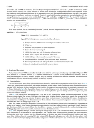
The energy output from a combined cycle power plant (CCPP) varying with the operating thermal
parameters like ambient pressure, vacuum, relative humidity, and relative temperature is
modelling using different approaches. The huge data obtained from the experimental readings is
found to be highly non-linear using the data visualization technique. The energy output from the
CCPP reduces linearly with the temperature and non-linearly with pressure. A mathematical
model is developed for the predictions of the energy output. Modelling using sequential API and
functional API based artificial neural network (SANN and FANN) having single hidden layer is
carried out. Finally, energy output modelling using sequential API and functional API based deep
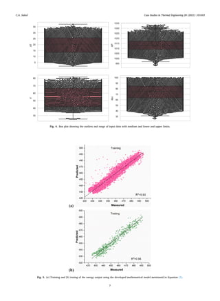
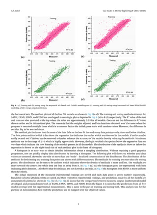
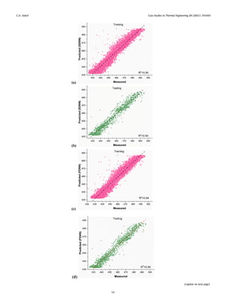
ANN (SDNN and FDNN) is also performed. The residuals of the predicted and experimental ob
servations indicate that the error is acceptable and it lies uniformly above and below the
regression line. The R-squared value of the mathematical model is 0.93 and 0.94 during training
and testing. The obtained R-squared value of the ANN and DNN using sequential and functional
API is 0.94. The training and testing of all the models are successful and these models have shown
a great compatibility in predicting the energy output of a CCPP. The ANN model with single layer
and deep layer has no difference in accuracy hence the former one is recommended as it is
computationally less expensive.
1. Introduction
In all over the world, electricity is the main driving soul of a current civilization and is the key essential resources to human ac
complishments. For the proper function of the economy and our society, we are in the requirement of a huge amount of electrical
power and due to continuous demand of electricity the use of combined cycle power plant (CCPP) is increasing day by day. To provide
needed amount of electricity to the human communities the power plants are established in large scale. The key concern in this favour
is the production of electrical power by keeping reliable and favourable power generation system. In thermal power plants generally,
thermodynamical methods are used to analyse the systems accurately for its operation. This method uses many number assumptions
and parameters to solve the thousands of nonlinear equations; whose elucidation takes too much effort and computational time or
sometimes it is difficulty to solve these equations without these assumptions [1,2].
To eradicate this barrier, in recent days the machine learning (ML) methods are commonly used as substitute to thermodynamical
methods and mathematical modelling to study the systems for random output and input patterns [1,3,4]. In ML approach, envisaging
an actual value called as regression is the most common problem. To control the system response and for predicting an actual numeric
value, the ML approach uses machine learning algorithms. Using ML approach and its algorithms, the many realistic and everyday
E-mail addresses: ahamedsaleel@gmail.com, ahamedsaleel@gmail.com.
Contents lists available at ScienceDirect
Case Studies in Thermal Engineering
journal homepage: www.elsevier.com/locate/csite
https://doi.org/10.1016/j.csite.2021.101693
Received 11 April 2021; Received in revised form 7 November 2021; Accepted 3 December 2021

2
problems can be elucidated as regression problems to improve prognostic models [5].
The Artificial Neural Networks (ANNs) is one of the methods of ML. Using ANNs the environmental conditions and nonlinear
relationships are considered as inputs of the ANNs model, and the power generates is considered as the output of the model. Using ANN
model, we can calculate the power output of the power plant by giving the various environmental conditions.
ANNs were proposed originally in the mid of 20th century as a human brain computational model. At that time, their use was
restricted due to the available of limited computational power and few theoretically unsolved problems. Though, they have been
applied and studied increasingly in recent days due to their availability if computational power and datasets [6]. In modern thermal
power plants, a huge quantity of parametric data is kept over long periods of time; hence, a big data created on the active data is
continuously readily available without any extra cost [7].
The present study deals with various ML regression approaches for an extrapolation study of a CCPP as a thermodynamic system.
The CCPP involves two heat recovery systems, one steam turbine, and two gas turbines. Using ML techniques, the calculation of
electrical power output of a CCPP is considered as a one real-life critical problem. For the economic operation and efficiency of a power
plant, the calculation of electrical power output for full and base load of a power plant is very important. It also helps to improve the
revenue from obtainable Megawatt hours (MWh). The gas turbine sustainability and reliability is highly depending on calculation of its
generation of power.
The output power of gas turbine mainly depends on the atmospheric parameters such as relative humidity, atmospheric pressure
and atmospheric temperature. The output power of a steam turbine has direct correlation with exhaust vacuum. The effects of at
mospheric disorders are deliberated in the literature for the calculation of electrical power (PE) by using ML intelligence systems i.e.,
ANNs [1,8,9]. Several investigations have deliberated ANN model to numerous engineering systems [10–17]. Many investigators
conveyed the reliability and feasibility of ANN models as analysis and simulation tool for different power plant components and
processes [18–25]. Comparatively limited studies have deliberated the use of steam turbine (ST) in a CCPP [3,7,26,27]. Back prop
agation modelling of nanofluids based on MXene nanoparticles was modelled by Afzal et al. [20] which provided an excellent pre
diction of the viscosity and shear stress of the nanofluid. A similar work on the battery Nusselt number, base pressure predictions at
sonic and supersonic numbers by the same authors is proposed in Refs. [21–25].
Using ANN model in Ref. [1] the various effects such as wind velocity and its direction, relative humidity, ambient pressure,
ambient temperature on the power plant are examined based on the measured information from the power plant. For varying local
atmospheric conditions, in Ref. [9] the ANN model is used to calculate the performance and operational parameters of a gas turbine. In
Refs. [8,26], researchers compared different ML methods to calculate the full load output of electrical power of a base load operated
CCPP.
The modelling of stationary gas turbine is also done by using ANNs. In Ref. [28], the ANN system is developed and effectively used
for studying the behaviours of gas turbine for different range of working points starting from full speed full load and no-load situations.
The radial basis function (RBF) and Multi-Layer Perception (MLP) networks are effectively used in Ref. [29] for finding start-up stage of
stationary gas turbine. In Refs. [30,31], authors used different designs of MLP method to estimate the electrical power output and
performance of the CCPP by using variable solvers, hidden layer configurations and activation functions.
For identification of gas turbine in Ref. [32], the Feed Forward Neural Networks (FFNNs) and dynamic linear models are compared
and found Neural Networks (NNs) as a prognosticator model to pinpoint superior enactments than the vigorous linear models. The
ANNs models are also effectively employed in isolation, fault detection, anomaly detection and performance analysis of gas turbine
engines [2,33,34]. In Refs. [35–37], CCPP total electrical energy power output is predicted by using FFNNs which is fully based on
novel trained particle swarm optimization method. They used atmospheric pressure, vacuum, relative humidity and ambient tem
perature as input factors to calculate hourly average power output of the CCPP. An ANN based ML processing tool and its predictive
approach is successfully used in Ref. [38] CCPPs to study and analyse the environmental impact on CCPP generation. In Ref. [39], the
Internet of Things (IoT) based micro-controller automatic information logger method is employed to accumulate environment data in
CCPPs. In Ref. [40], the researchers estimated the electrical power output by employing Genetic Algorithm (GA) method for the design
of multilayer perception (MLP) for CCPPs.
Additionally, in the literature, numerous studies [41–47] have been carried to envisage consumption of electrical energy by using
ML intelligence tools, also little studies i.e. [1] carried out related to the calculation of overall electrical power of a CCPP with a heating
system, one steam turbine and three gas turbines. In Ref. [48], authors used an extreme Learning Machine (ELM) as the base regression
model to analyse performance of the power plant in a vigorous atmosphere that can update regression models autonomously to react
with abrupt or gradual environmental changes. In Ref. [49], the authors used Cuckoo Search based ANN to predict output electrical
energy of gas turbine and combined steam mechanisms in order to yield more reliable mechanisms. However, for the first-time deep
learning model based on sequential and functional API neural network modelling is carried out. For the comparison, ANN modelling
based on sequential and functional API is performed. A mathematical model is also developed apart from the soft computing method.
The work adopted for forecasting of CCPP data is started with the description of the CCPP system in section 2. Section 3 discusses the
ANN and DNN method adopted for CCPP modelling. The mathematical modelling, data visualization, ANN and DNN modelling results
are in detail provided in section 4. Conclusions are provided at the end in section 5.
2. CCPP system
A combined cycle power plant (CCPP) consists of steam turbines (ST), heat recovery steam generators (HTSG) and gas turbines
(GT). In CCPP, the ST and electricity generated by gas is combined in lone cycle, and is relocated from one turbine to another [18]. A
GT in a combined cycle system not only produce electrical power (EP) but also produces equally hot gasses. Directing these gases
C.A. Saleel

3
through a liquid cooled heat exchanger that generates steam, this can be revolved into EP with a coupled generator and ST. Therefore,
a GT generator produces electricity and leftover heat of the exhaust gases is employed to generate steam and additionally produces
electricity through a ST. All around the world, the similar kind of power plants are fitted in increasing numbers where the more
substantial quantities of natural gas are available [19]. For this study the set of data’s are taken from CCPP-1, which is considered with
a small producing capacity of 480 MW, made up of one 160 MW ABB ST, 2 dual pressure heat recovery steam generators (HRSG) and
two 160 MW ABB 13E2 GTs are illustrated in Fig. 1. The load on GT is very sensitive to the atmospheric conditions; essentially relative
humidity (RH), atmospheric pressure (AP) and ambient temperature (AT). On the other hand, the load on ST is very delicate to the
steam exhaust pressure or vacuum. In this study, the factors of both ST and gasses are correlated with exhaust steam pressure and
ambient conditions, are employed as I/P variables as data set. The generation of EP by both STs and gas is employed as a key variable in
the dataset.
All the key variable and I/P variables are defined as below related to hourly average data collected from the measurement sensor
points are denoted in Fig. 1.
1) Ambient Temperature (AT): This I/P variable is restrained in Celsius in degrees as it changes among 1.81 ◦
C and 37.11 ◦
C.
2) Relative Humidity (RH): This I/P variable is restrained as percentage from 25.56% to 100.16%.
3) Vacuum (Exhaust Pressure of Steam, V): This I/P variable is restrained in cm Hg with the variation of 25.36 cm Hg to 81.56 cm Hg.
4) Atmospheric Pressure (AP): This I/P variable is restrained in units of minibar (mbar) with the variation of 992.89 mbar–1033.30
mbar.
5) Full Load EP output (PE): This variable is used as a key variable in the dataset. It is calculated in MW with the variation of 420.26
ME to 495.76 MW.
3. Modelling of ANN and DNN
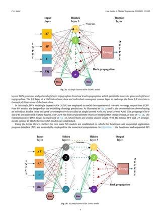
A Neural Network (NN) is a numerical tool that creates calculations built on data from the past. An ANN comprises of various inputs
(I/P) sources that yield inputs built on earlier described data. Then and most importantly, the unseen layers use backpropagations
(BPs) to make the most of neuron’s loads to improve the NNs training. Finally, the output (O/P) layers which are calculated based on
the unseen layer and I/P information. A multi-layered network (MLN) in ANN is known as the backpropagation (BP) NN i.e., most
frequently used. MLN is the utmost common and basic method employed for controlled NNs training by changing and altering the non-
linear correlation between O/P and I/P BP works. In common, the testing and training are two stages of the BP network. In the process
of training, the network is provided with essential classifications and I/Ps. For example, the I/P could be a programmed image of a face
and a program that relates to the individual name that explain the O/P. The Deep Learning (DL) NNs are the key example of a multi-
output or single regression problem algorithm. The various DL archives are available readily to describe and calculate NN models for
multi-O/P regression tasks. DNN is a network built on ANN approach comprising of a group of unseen layers among the O/P and I/P
Fig. 1. Layout of CCPP [18].
C.A. Saleel

4
layers. DNN generates and gathers high level topographies from low level topographies, which permit the source to generate high level
topographies. The I/P layer of a DNN takes basic data and individual consequent unseen layer to exchange the basic I/P data into a
theoretical illustration of the basic data.
In this study, DNN and single layered ANN (SLNN) are employed to model the experimental relevant to energy output from CCPP.
Four NN models are designed for the modelling of energy predictions. As illustrated in Fig. 2a and b, the two models are shown having
an individual hidden layer and deep layers respectively so called as single layered ANN and deep layered ANN. The groupings of O/P
and I/Ps are illustrated in these figures. The CCPP has four I/P parameters which are modelled for energy output, as seen in Fig. 2a. The
representation of DNN model is illustrated in Fig. 2b, where there are several unseen layers. With the similar O/P and I/P arrange
ments, similar to SLNN the four DNN models are established.
Using the Keras library, further the two main NN models are established, in which the functional and sequential application
program interface (API) are successfully employed for the numerical computations. In Algorithm 1, the functional and sequential API
Fig. 2a. a) Single layered ANN (SANN) model.
Fig. 2b. b) Deep layered ANN (DNN) model.
C.A. Saleel

5
model of the ANN and DNN are mentioned. Hence, in the present experimental data, the total 2 × 2 = 4, models are developed. Further
inclusive network topology with varying from 1 to 10 neurons in the middle layer are adopted for numerical data regression. In each
data, the feature predictions are very different, so we reassigned it to two fully associated layers with different sizes of O/P, the number
of dimensions in each feature predictions are reduced. These O/Ps could be deliberated as multiplication matrix for high level I/P data
concept. To access the performance of the models, the R-squared (R2
) is calculated using Equation (1). The value of R2
lies between
0 and 1. The model with highest fit, is represented by R2
= 1, while failure is model is when R2
= 1, Closer to R2
= 1 shows better fitness
of model with the actual values.
R =
̅̅̅̅̅̅̅̅̅̅̅̅̅̅̅̅̅̅̅̅̅̅̅̅̅̅̅̅̅̅̅̅̅̅̅̅̅̅̅̅̅̅̅̅̅̅̅̅̅
1 −
∑c
a=1
(
Yt − Yp
)2
∑c
a=1
(
Yt(mean) − Yp
)2
√
√
√
√ (1)
In the above equation, n is the values totally recorded, Yt and Yp indicated the predicted value and true value.
Algorithm 1. DNN/ANN Model
4. Results and discussion
The input parameters of CCPP considered in this study which affect the net hourly electrical energy output (PE) in Megawatt (MW)
of the plant are: 1) AP (ambient pressure) 2) AT (ambient temperature) 3) V (exhaust vacuum) 4) RH (relative humidity). Based on
these input parameters the energy output is recorded which is available in UCI machine learning repository. Data visualization,
modelling using different approaches, and residuals are analysed in detail.
4.1. Data visualization
The data visualization of the entire input parameters and the energy output (PE) varying for their entire range is shown in Fig. 3.
The sea born library is used to perform this huge amount of data set. In these kinds of numerical variables where the data variations are
huge and highly non-linear, the data visualization helps in gaining the insights to data dependencies. The snspairplot command is used
for the plot obtained in Fig. 3. The diagonal bar element represents the histogram of the data densities. The diagonal histograms are to
know at which particular data point the density is more or less. Obviously from the figure the density variations of range of data points
are not similar for any attribute.
From Fig. 3 the energy output with temperature (AT) is seen to vary quite linearly. A good and smooth trendline can be easily
shown over their relation. The vacuum (V) is largely non-linear as the variation of energy output is not smooth. The pressure (AP) is
seen to arbitrarily affect the energy output as the pattern is not of any particular nature. The humidity (RH) is more absurd than the
pressure and looks to take place over the entire space of the co-ordinate. Hence vacuum and temperature are most important input
parameters that effect the energy output of the CCPP.
A box plot is a sort of chart that is frequently employed for the data analysis elucidation in descriptive statistics (famous also as
whisker or the box plot). In the box plot, the data skewness is displayed in averages and percentiles or quartiles and visually depicts the
data distribution which is of numerical form. Box plots deliver a summary of numerical data set in five-number, including median,
third (upper) quartile, first (lower) quartile, maximum score and the minimum score.
In Fig. 4 the box plot of the input variables affecting the energy output of the CCPP is shown individually. The mean values are
easily discoverable for the data set at the centre with a black line. The band in the middle represents the lower and upper quartiles of
the numerical values of the variables that 50% of data lie around it. The lower and upper horizontal lines show the lower and upper
range of the whiskers where the remaining 50% data is located. The datapoints falling above or below this show the outliers which
make the prediction of output slightly complicated. For temperature (AT) the outliers do not exist and hence the data distribution is
C.A. Saleel

6
appropriate. For pressure (AP) the outliers are clearly visible above the max whisker and slightly below the lower whisker. For vacuum
(V) the data is also quite uniform with some data points in the range of min whiskers. However, the inter quartile range is wider than
the previous variables. The humidity (RH) is some what different than the other variables. The data is located equally up to the max
whiskers and the data in the lower whisker is arranged largely indicating a greater skewness.
4.2. Data modelling
4.2.1. Mathematical modelling
In the initial phase of this work, a mathematical model is developed using the input variables to fit the available energy output of
the CCPP. Using the method of data fitting the following mathematical model provided in Equation (1) is obtained. For developing this
model only 85% of the data is considered as a part if training. The remaining 15% of data is used to validate the proposed model which
is actually to test it. The training and testing predictions made by the model in the respective stage for the energy output is shown in
Fig. 5 (a) and (b) respectively.
The coefficient of determination (R2
) value during the training is 0.93 and in testing it is 0.94 which is highly satisfying. The
experimental and predictions made by the model can hence be used for the predictions of energy output of CCPP using the input
parameters mentioned in this article. The outliers existing in the energy output are away from the trendline which are clearly visible
from the figure itself. Due to these outliers the accuracy is not 100%.
Fig. 3. The dependency of input thermal parameters with the energy output.
C.A. Saleel

7
Fig. 4. Box plot showing the outliers and range of input data with medium and lower and upper limits.
Fig. 5. (a) Training and (b) testing of the energy output using the developed mathematical model mentioned in Equation (2).
C.A. Saleel

8
PE = 675 + 0.005*AT*RH + 0.0006*AT3
+ 7.3e − 6*AT*AP2
− 0.15*AP − 10.5*AT − 0.004*V*RH (2)
4.2.2. Neural network modelling
In this section the neural network (NN) modelling of data using the sequential API (application program interface) based single
layered ANN (artificial NN) - SANN and functional API based single layered ANN - FANN is initially presented. Later, sequential API
based deep i.e., 5 hidden layers NN (DNN) – SDNN and functional API based DNN - FDNN modelling results are analysed. For the entire
modelling process a 5-fold cross validation method was adopted. In Table 1 the summary of network structure is mentioned.
Fig. 6 shows the training and testing results of the SANN algorithm when it is feed with the energy output data recorded with the
experimental sensors. From Fig. 6 (a) and (b) it can be noted that the R2
value of the SANN model is 0.93 and 0.94 respectively during
the training and testing of the model. The predictions from SANN model and the mathematical model are same hence they stand
together. The results presented here are obtained after serval computational experimentations. The ANN model neurons in the hidden
layer were varied from 1 to 12 to note the highest accuracy. It was found that the model with 8 neurons in the layer was with the
highest accuracy, hence it was adopted throughout. The pattern of 4-8-1 has hence proved to be most suitable.
The functional API based ANN (FANN) modelling having a single hidden layer with 8 as the optimized number of neurons in the
hidden layer is carried out. The training and testing results of the energy output using the FANN framework is performed. The 4-8-1
structure of the FANN is run for more than 1000 epochs to obtain the lowest error combined for training and testing. The error is
minimized with the back propagation modelling here wherein the weights and bias values are adjusted accordingly. The R2
value of the
FANN model is 0.94 each respectively during the training and testing of the model. This is slightly enhanced accurate than the SANN
model.
The data points of the outliers are very few in numbers as can be noted from Fig. 6 (c) and 6 (d). The pink circles representing each
single data point having energy output of the CCPP is densely oriented towards the trendline in black colour. The data points acting as
outliers are the reason for accuracy less than 100%. These outliers can be easily removed, but there are chances of over-fitting of the
model. No outlier is noted below the trendline, hence only in the max whisker of the data point the modelling issues are guessed. The
single layered ANN models are however have shown a great significance of their ability to predict the energy of the CCPP. In literature
to a certain extent ANN models are used while rarely other models like K-nearest neighbour, rando forest, linear regression models are
reported in the field of energy output modelling.
The sequential API based DNN (SDNN) modelling of energy output of CCPP using the input neurons as temperature, humidity,
pressure, and vacuum are performed as a part of deep learning method. The predictions obtained using the deep learning algorithm are
shown in Fig. 7. The training carried using the experimental data is compared once the model is mapped properly i.e., when the error
minimized between them with the adjustments of weights and bias functions. The experimental and SDNN model output are compared
in Fig. 7 (a) which indicates that the predictions made are appropriate and accurate. The R2
value of the SDNN model is 0.94 which is
again in-line with the previous mathematical model, SANN, and FANN framework. The outliers are again in the same range outside the
trendline and above it indicating the same data pint being reducing the accuracy to less than 100%. The testing accuracy obtained
using the trained SDNN model is shown in Fig. 7 (b). The testing R2
value of the SDNN model is 0.94 which is same with the trained
model. Hence the DNN model is equivalently capable of the proper predictions. If huge data set is fed to this deep model, a highly
complex and sensitive variations in the energy output could also be easily predicted.
Fig. 7(c–d) illustrates the training and testing of the functional API based deep ANN model (FDNN) for CCPP energy output based
on input thermal parameters. The training output obtained after 1000 iterations are noted and compared with the experimental output.
Fig. 7 (c) shows that the training of the FDNN model is successful. The R2
value of the FDNN model is 0.94 and is in-line with the
remaining models. If a keen observation is made between the Fig. 7 to 10 obtained from the SANN, FANN, SDNN, and FDNN models it
is observed that the data points in the range of 430–440 MW energy output are slightly skewed. For ANN model the distribution is
homogenous while in DNN models only the density of data is more at the corners.
However, a comparison between these models indicates that the no one is superior to each other comparatively. The accuracy is in
the same range. The outliers are also similarly distributed. The testing of the five trained models also indicates the same accuracy. The
structure of the deep models is finalized to 4-5-1 where if any further increase in the number of deep hidden layers from 5 to 10, no
change in accuracy is noted. However, an important aspect that can be compared is the computational capability of all the models.
ANN model having single hidden layer does not required heavy computations as deep ANN. Hence, the computational cost of the DNN
models and the respective power consumed for this is more than the ANN models.
4.2.3. Residuals from sequential and functional API based ANN and DNN
A residual plot shows the measurement of the vertical lack of a data point on the regression line. The best fit of a data set is denoted
by the regression line. The lines can be seen as averages; several data points are on the line and others are missed. A plot with residual
values on the vertical axis displays the difference between the observed and predicted values and the independent variable is shown on
Table 1
Models used for forecasting of CCPP data.
Model Hidden Layers Neurons
SANN 1 8
FANN 1 8
SDNN 5 6
FDNN 5 6
C.A. Saleel

9
the horizontal axis. The residual plots of all the four NN models are shown in Fig. 8(a–d). The training and testing residuals obtained for
SANN, FANN, SDNN, and FDNN are overlapped in one single plot as depicted in Fig. 8 (a) to 8 (d) respectively. The R2
value of the test
and train are also provided at the top where the vales are approximately 0.93 for all models. One can ask the difference in R2
value
shown earlier and in this residual plot. The reason is that the weights adjusted and bias functions obtained won’t be same when the
program is executed multiple times which is a common fact as the initial guess starts with random values. However, the difference is
not that big to be worried about.
The residual plot indicates that the most of the data falls on the best fit line and many data points evenly above and below this line.
The data points residual which is far above the regression line indicates the outlier which are observed in the models. if outlier can be
easily located and if desired can be removed to further enhance the accuracy of the models thereby reducing the residuals. Maximum
residuals are in the range of ±10 which is highly appreciable. However, the high residuals data points below the regression line are
very less which indicate the slow learning of the models present in all the models. The distribution of the residuals above or below the
regression is shown on the right-hand side of each residual plot in the form of histogram.
A histogram is an easy way to obtain detailed information about a sampling distribution. Without requiring a good graphics
programme, one can quickly display data distribution by drawing a histogram. The following plot will show you whether your data
values are centered, skewed to one side or more than one ‘mode’ - localized concentration of the distribution. The distribution of the
residuals for both testing and training data points are shown with different colours. The residuals for training are more than the testing
points. The distribution can be seen to be uniform which indicates where the density of residuals is more and less. The residuals are
more towards the centre line while they are less as away from it. In Fig. 8 (a)–(d) the histogram plots are represented with bars
indicating their densities. This shows that the residuals are not skewed at one side. In Fig. 8 the histogram from FDNN is more uniform
then the others.
The actual variations of the measured experimental readings are sorted and each data point is given number sequentially.
Randomly selected 20 data points are opted and their respective experimental readings, and predictions made by all the models are
comparatively plotted as shown in Fig. 8(e–f). Fig. 8(e–f) shows that the comparison between measured output, mathematical model
developed, and proposed framework of SANN, FANN, SDNN, and FDNN. From the figure it is seen that the predictions from all five
models overlap with the experimental measurements. This is same in the part of training and testing both. This analysis was for the
purpose of demonstration how well the predictions are in mapped with the observed values.
Fig. 6. (a) Training and (b) testing using the sequential API based ANN (SANN) modelling and (c) training and (d) testing using functional API based ANN (FANN)
modelling of the energy output predictions.
C.A. Saleel

10
(caption on next page)
C.A. Saleel

11
5. Conclusions
In this work the mathematical modelling and neural network (NN) modelling of the energy output data belonging to the combined
cycle power plant (CCPP) is carried out. The experimental readings obtained from the CCPP are recorded with ambient temperature,
pressure, humidity, and vacuum as the independent variables. A mathematical model is developed and ANN and DNN models based on
sequential and functional API approach are adopted for the regression. The following important conclusions are drawn.
• The data visualization of the variables indicate that temperature and pressure are the most significantly and linearly affecting the
performance of CCP energy output in MW. The other two parameters haphazardly effect the energy output.
Fig. 7. (a) Training and (b) testing using the sequential API based DNN (SDNN) modelling and (c) training and (d) testing using functional API based DNN (FDNN)
modelling of the energy output predictions.
Fig. 8. Residual’s plot and its histogram obtained during the training and testing of CCPP energy output using (a) SANN (b) FANN (c) SDNN, and FDNN framework.
Comparison between the predictions made by the NN models, mathematical model, and the experimental measurements during (e) training (f) testing.
C.A. Saleel

12
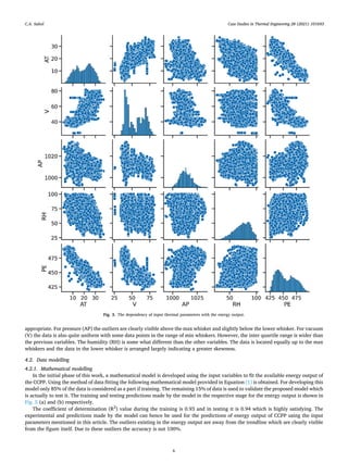
• The box plot variations indicate that the outliers exist in pressure and humidity parameters while in the temperature and vacuum
the variables are in the min and max whisker and interquartile range.
• The mathematical model developed is accurate to predict the energy output of the power plant. Hence this model can be used for
forecasting and when this model is compared with the NN models, the accuracy is similar.
• The four NN models of ANN and DNN developed are in the same range of accuracy and are successfully trained and tested with a
split up of 80% and 20% data.
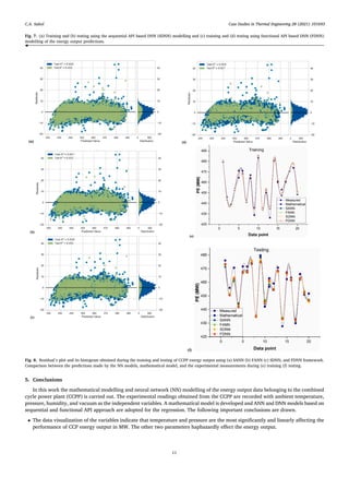
• The residual plot for al the NN models proposed indicated that the distribution of error is thought in the same range. This is also
confirmed by the sample distribution using histogram.
The work can be extended to apply various machine learning models like support vector machines, gradient boosting algorithms,
ensemble techniques and many more. The mathematical model developed will help in obtaining the optimization of CCPP energy
output. In this regard several latest algorithms available can be easily chosen. Correlation matrix indicating the dependency and
relationship between the factors can also be analysed in future.
Authorship contributions
Category 1
Conception and design of study: C Ahamed Saleel.
Acquisition of data: C Ahamed Saleel.
Analysis and/or interpretation of data: C Ahamed Saleel.
Category 2
Drafting the manuscript: C Ahamed Saleel.
Revising the manuscript critically for important intellectual content: C Ahamed Saleel.
Category 3
Approval of the version of the manuscript to be published (the names of all authors must be listed): C Ahamed Saleel.
Declaration of competing interest
The authors declare that they have no known competing financial interests or personal relationships that could have appeared to
influence the work reported in this paper.
Acknowledgments
The author extends his appreciation to the Deanship of Scientific Research at King Khalid University, Saudi Arabia for funding this
work through Research Group Program under Grant No: RGP 2/105/41.
References
[1] U. Kesgin, H. Heperkan, Simulation of thermodynamic systems using soft computing techniques, Int. J. Energy Res. 29 (2005) 581–611.
[2] A. Samani, Combined cycle power plant with indirect dry cooling tower forecasting using artificial neural network, Decis. Sci. Lett. 7 (2) (2018) 131–142.
[3] P.R. Norvig, S.A. Intelligence, A modern approach, Manuf. Eng. 74 (1995) 111–113.
[4] E. Rich, K. Knight, Artificial Intelligence, McGraw-Hill, New York, 1991.
[5] H.A. Güvenir, Regression on feature projections, Knowl. -Based Syst. 13 (2000) 207–214.
[6] M.T. Hagan, H.B. Demuth, M.H. Beale, Orlando De Jesus. Neural Netw. Des, second ed., Cengage Learn, 2014.
[7] A. Dehghani Samani, Combined cycle power plant with indirect dry cooling tower forecasting using artificial neural network, Decis. Sci. Lett. 7 (2018) 131–142.
[8] H. Kaya, P. Tüfekci, F.S. Gürgen, Local and global learning methods for predicting power of a combined gas & steam turbine, in: International Conference on
Emerging Trends in Computer and Electronics Engineering (ICETCEE’2012), 2012. Dubai, March 24–25.
[9] M. Fast, M. Assadi, S. Deb, Development and multi-utility of an ANN model for an industrial gas turbine, Appl. Energy 86 (1) (2009) 9–17.
[10] D. Jahed Armaghani, M.F. Mohd Amin, S. Yagiz, R.S. Faradonbeh, R.A. Abdullah, Prediction of the uniaxial compressive strength of sandstone using various
modeling techniques, Int. J. Rock Mech. Min. Sci. 85 (2016) 174–186.
[11] H. Moayedi, D. Jahed Armaghani, Optimizing an ANN model with ICA for estimating bearing capacity of driven pile in cohesionless soil, Eng. Comput. 34
(2018) 347–356.
[12] A. Afzal, J.K. Bhutto, A. Alrobaian, A.R. Kaladgi, S.A. Khan, Modelling and computational experiment to obtain optimized neural network for battery thermal
management data, Energies 14 (2021) 7370, https://doi.org/10.3390/en14217370.
[13] A. Afzal, S. Alshahrani, A. Alrobaian, A. Buradi, S.A. Khan, Power plant energy predictions based on thermal factors using ridge and support vector regressor
algorithms, Energies 14 (2021) 7254, https://doi.org/10.3390/en14217254.
[14] S. Tamilselvi, S. Gunasundari, N. Karuppiah, A. Razak Rk, S. Madhusudan, V.M. Nagarajan, T. Sathish, M.Z.M. Shamim, C.A. Saleel, A. Afzal, A review on
battery modelling techniques, Sustain. Times 13 (2021) 1–26, https://doi.org/10.3390/su131810042.
[15] A. Chandrashekar, B.V. Chaluvaraju, A. Afzal, D.A. Vinnik, A.R. Kaladgi, S. Alamri, A.S. C, V. Tirth, Mechanical and corrosion studies of friction stir welded nano
Al2O3 reinforced Al-Mg matrix composites: RSM-ANN modelling approach, Symmetry (Basel). 13 (2021) 537, https://doi.org/10.3390/sym13040537.
[16] R. Pinto, A. Afzal, L. D’Souza, Z. Ansari, A.D. Mohammed Samee, Computational fluid dynamics in turbomachinery: a review of state of the art, Arch. Comput.
Methods Eng. 24 (2017) 467–479, https://doi.org/10.1007/s1183.
[17] A. Afzal, Z. Ansari, A. Faizabadi, M. Ramis, Parallelization strategies for computational fluid dynamics software: state of the art review, Arch. Comput. Methods
Eng. 24 (2017) 337–363, https://doi.org/10.1007/s11831-016-9165-4.
[18] C. Wan, Z. Xu, P. Pinson, Z.Y. Dong, K.P. Wong, Optimal prediction intervals of wind power generation, IEEE Trans. Power Syst. 29 (2014) 1166–1174.
[19] F. Bizzarri, M. Bongiorno, A. Brambilla, G. Gruosso, G.S. Gajani, Model of photovoltaic power plants for performance analysis and production forecast, IEEE
Transact. Sustain. Energy 4 (2013) 278–285.
C.A. Saleel

13
[20] A. Afzal, K.M.Y. Navid, R. Saidur, R.K.A. Razak, R. Subbiah, Back propagation modeling of shear stress and viscosity of aqueous Ionic - MXene nanofluids,
J. Therm. Anal. Calorim. (2021), https://doi.org/10.1007/s10973-021-10743-0.
[21] I. Mokashi, A. Afzal, S.A. Khan, N.A. Abdullah, M.H. Bin Azami, R.D. Jilte, O.D. Samuel, Nusselt number analysis from a battery pack cooled by different fluids
and multiple back-propagation modelling using feed-forward networks, Int. J. Therm. Sci. (2021) 106738, https://doi.org/10.1016/j.ijthermalsci.2020.106738.
[22] A. Afzal, A. Aabid, A. Khan, S. Afghan, U. Rajak, T. Nath, R. Kumar, Response surface analysis , clustering , and random forest regression of pressure in suddenly
expanded high-speed aerodynamic flows, Aero. Sci. Technol. 107 (2020) 106318, https://doi.org/10.1016/j.ast.2020.106318.
[23] A. Afzal, S.A. Khan, T. Islam, R.D. Jilte, A. Khan, M.E.M. Soudagar, Investigation and back-propagation modeling of base pressure at sonic and supersonic Mach
numbers, Phys. Fluids 32 (2020), 096109, https://doi.org/10.1063/5.0022015.
[24] A. Afzal, C.A. Saleel, I.A. Badruddin, T.M.Y. Khan, S. Kamangar, Z. Mallick, O.D. Samuel, M.E.M. Soudagar, Human thermal comfort in passenger vehicles using
an organic phase change material– an experimental investigation, neural network modelling, and optimization, Build. Environ. 180 (2020) 107012, https://doi.
org/10.1016/j.buildenv.2020.107012.
[25] A. Razak, A. Afzal, A.M. Manokar, D. Thakur, U. Agbulut, S. Alshahrani, A.S. C, R. Subbiah, Integrated Taguchi-GRA-RSM optimization and ANN modelling of
thermal performance of zinc oxide nanofluids in an automobile radiator, Case Stud. Therm. Eng. 26 (2021) 101068, https://doi.org/10.1016/j.
csite.2021.101068.
[26] P. Tüfekci, Prediction of full load electrical power output of a base load operated combined cycle power plant using machine learning methods, Int. J. Electr.
Power Energy Syst. 60 (2014) 126–140.
[27] L.X. Niu, X.J. Liu, Multivariable generalized predictive scheme for gas turbine control in combined cycle power plant, IEEE Conf. Cybern. Intellig. Syst. (2008)
791–796, 21-24 September 2008.
[28] M. Rahnama, H. Ghorbani, A. Montazeri, Nonlinear identification of a gas turbine system in transient operation mode using neural network, in: 4th Conference
on Thermal Power Plants (CTPP), IEEE Xplore, 2012.
[29] M.H. Refan, S.H. Taghavi, A. Afshar, Identification of heavy duty gas turbine startup mode by neural networks, in: 4th Conference on Thermal Power Plants
(CTPP), IEEE Xplore, 2012.
[30] Ivan Lorencin, Zlatan Car, Kudláček Jan, Vedran Mrzljak, Nikola Anđelić, Sebastijan Blažević, Estimation of combined cycle power plant power output using
multilayer perceptron variations, in: 10th International Technical Conference-Technological Forum, 2019, pp. 94–98.
[31] Ali Alperen Islikaye, Aydin Cetin, Performance of ML methods in estimating net energy produced in a combined cycle power plant, in: 2018 6th International
Istanbul Smart Grids and Cities Congress and Fair (ICSG), IEEE, 2018, pp. 217–220.
[32] M. Yari, M.A. Shoorehdeli, V94.2 gas turbine identification using neural network, in: First RSI/ISM International Conference on Robotics and Mechatronics
(ICRoM), IEEE Xplore, 2013.
[33] A. Kumar, A. Srivastava, A. Banerjee, A. Goel, Performance based anomaly detection analysis of a gas turbine engine by artificial neural network approach, in:
Procee. Annual Conference of the Prognostics and Health Management Society, 2012.
[34] S.S. Tayarani-Bathaie, Z.N. Sadough Vanini, K. Khorasan, Dynamic neural network-based fault diagnosis of gas turbine engines, Neurocomputing 125 (11)
(2014) 153–165.
[35] M. Rashid, K. Kamal, T. Zafar, Z. Sheikh, A. Shah, S. Mathavan, Energy prediction of a combined cycle power plant using a particle swarm optimization trained
feedforward neural network, in: 2015 International Conference on Mechanical Engineering, Automation and Control Systems (MEACS), IEEE, 2015, pp. 1–5.
[36] Elkhawad Ali Elfaki, Hassan Ahmed, Ahmed, Prediction of electrical output power of combined cycle power plant using regression ANN model, J. Power Energy
Eng. 6 (12) (2018) 17.
[37] Bayram Akdemir, Prediction of hourly generated electric power using artificial neural network for combined cycle power plant, Int. J. Electr. Energy 4 (2)
(2016) 91–95.
[38] Md Hassanul Karim Roni, Muhammad Abdul Goffar Khan, An artificial neural network based predictive approach for analyzing environmental impact on
combined cycle power plant generation, in: 2017 2nd International Conference on Electrical & Electronic Engineering (ICEEE), IEEE, 2017, pp. 1–4.
[39] K. Uma, M. Swetha, M. Manisha, S. Revathi, A. Kannan, IOT based environment condition monitoring system, Indian J. Sci. Technol. 10 (2017).
[40] Ivan Lorencin, Nikola Anđelić, Vedran Mrzljak, Zlatan Car, Genetic algorithm approach to design of multi-layer perceptron for combined cycle power plant
electrical power output estimation, Energies 12 (22) (2019) 4352.
[41] G.K.F. Tso, K.K.W. Yau, Predicting electricity energy consumption: a comparison of regression analysis, decision tree and neural networks, Energy 32 (9) (2007)
1761–1768.
[42] A. Azadeh, M. Saberi, O. Seraj, An integrated fuzzy regression algorithm for energy consumption estimation with non-stationary data: a case study of Iran,
Energy 35 (6) (2010) 2351–2366.
[43] L. Ekonomou, Greek long-term energy consumption prediction using artificial neural networks, Energy 35 (2) (2010) 512–517.
[44] J. Che, J. Wang, G. Wang, An adaptive fuzzy combination model based on self-organizing map and support vector regression for electric load forecasting, Energy
37 (1) (2012) 657–664.
[45] K. Kavaklioglu, Modeling and prediction of Turkey’s electricity consumption using support vector regression, Appl. Energy 88 (2011) 368–375.
[46] P.C.M. Leung, E.W.M. Lee, Estimation of electrical power consumption in subway station design by intelligent approach, Appl. Energy 101 (2013) 634–643.
[47] M.R. Alrashidi, K.M. El-Naggar, Long term electric load forecasting based on particle swarm optimization, Appl. Energy 87 (2010) 320–326.
[48] Rui Xu, WeiZhong Yan, Continuous modeling of power plant performance with regularized extreme learning machine, in: 2019 International Joint Conference
on Neural Networks (IJCNN), IEEE, 2019, pp. 1–8.
[49] Sankhadeep Chatterjee, Nilanjan Dey, Amira S. Ashour, Cornelia Victoria Anghel Drugarin, Electrical energy output prediction using cuckoo search based
artificial neural network, in: Smart Trends in Systems, Security and Sustainability, Springer, Singapore, 2018, pp. 277–285.
C.A. Saleel

Total enegy forecasting using deep learning

More Related Content

Similar to Total enegy forecasting using deep learning

More from JNTUK KAKINADA

Recently uploaded

Total enegy forecasting using deep learning