Topic 6 Graphic Transformation and Viewing.ppt

Topic 6 Graphic Transformation and
viewing
Dr. Collins Oduor
Kenyatta University

Overview
 Why transformations?
 Basic transformations:
 translation, rotation, scaling
 Combining transformations
 homogenous coordinates, transform. Matrices
 First 2D, next 3D

Transformations
image
train
world
wheel
modelling…
instantiation…
viewing…
animation…

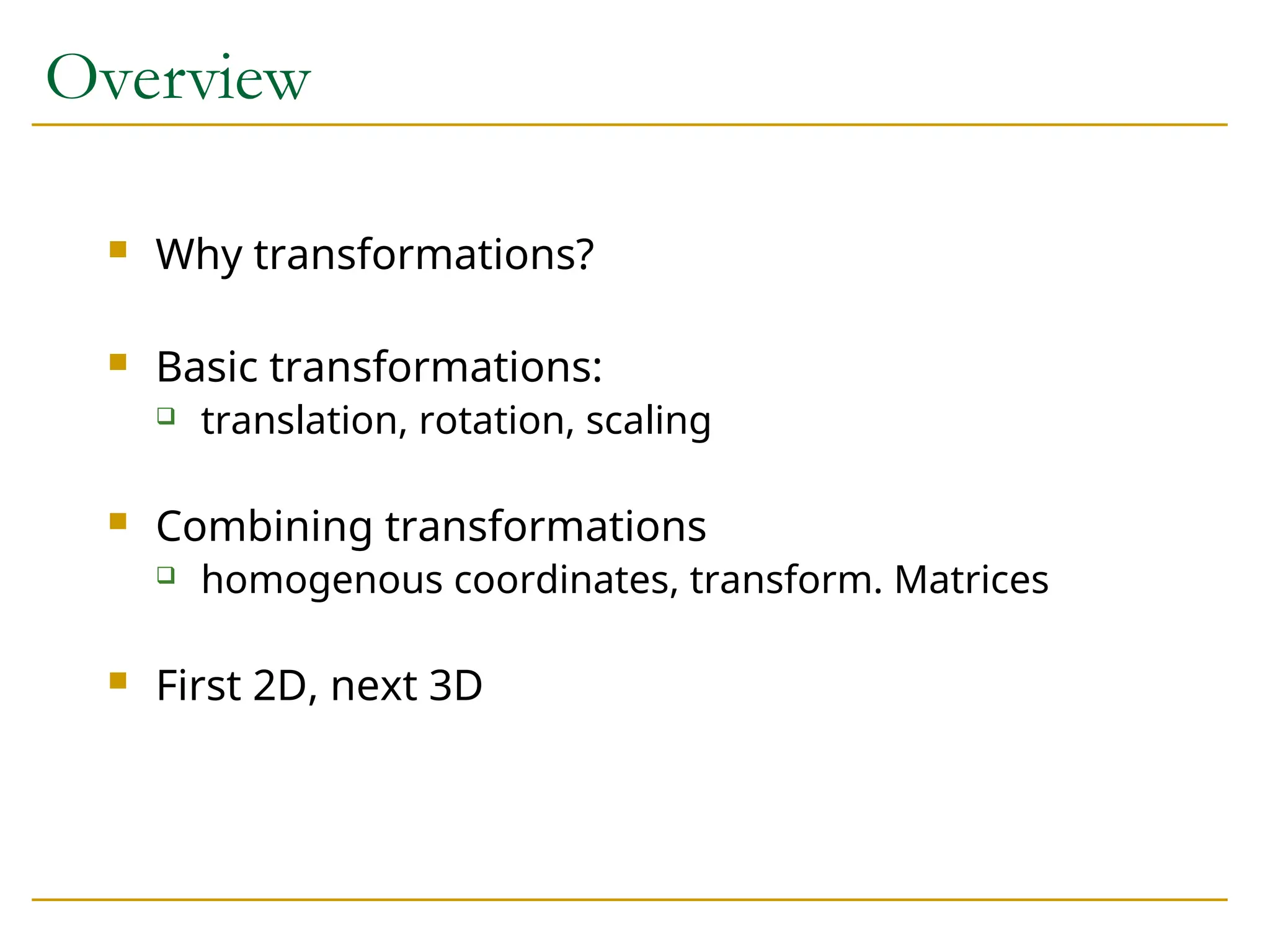
Why transformation?
 Model of objects
world coordinates: km, mm, etc.
Hierarchical models::
human = torso + arm + arm + head + leg + leg
arm = upperarm + lowerarm + hand …
 Viewing
zoom in, move drawing, etc.
 Animation

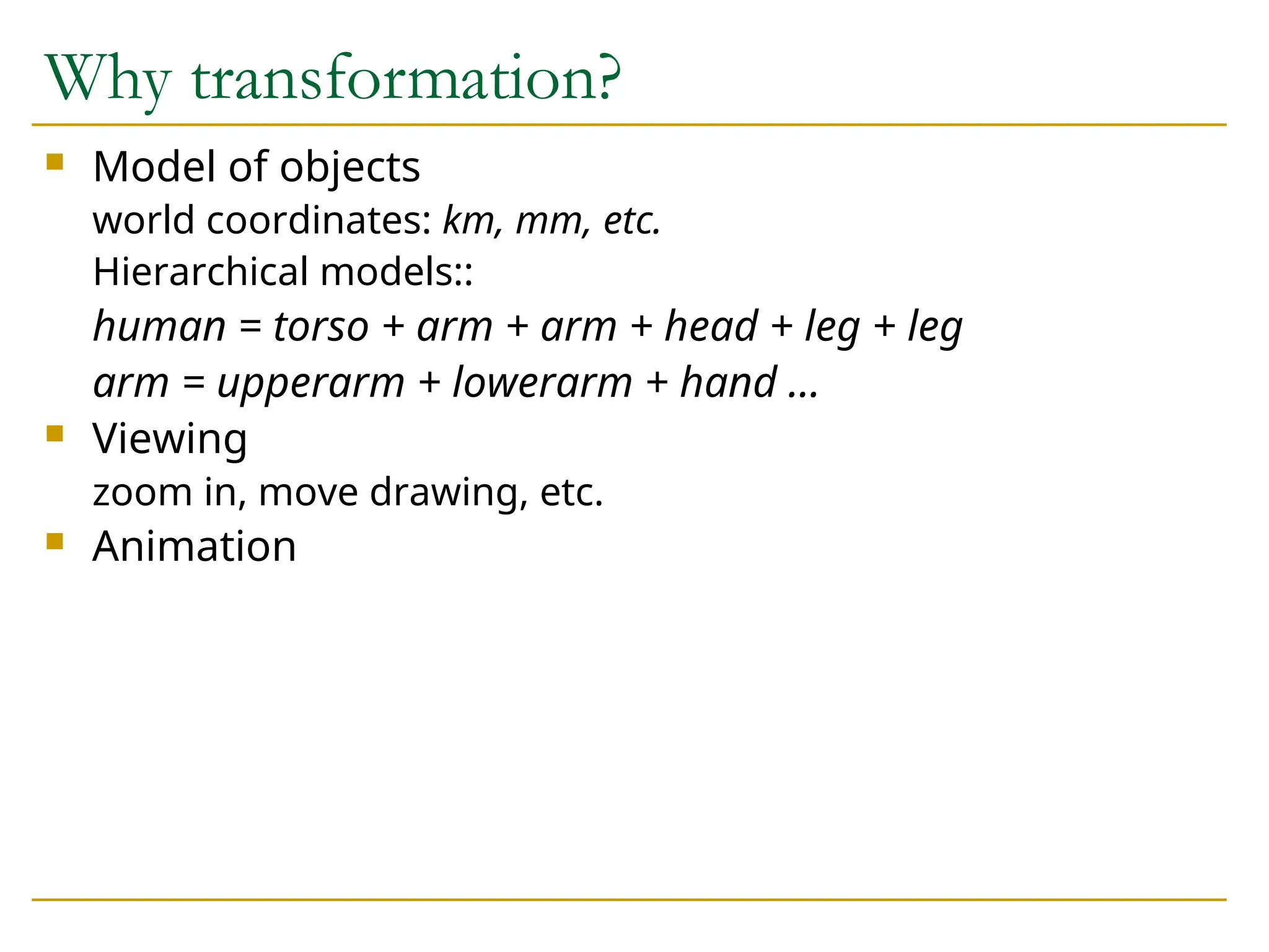
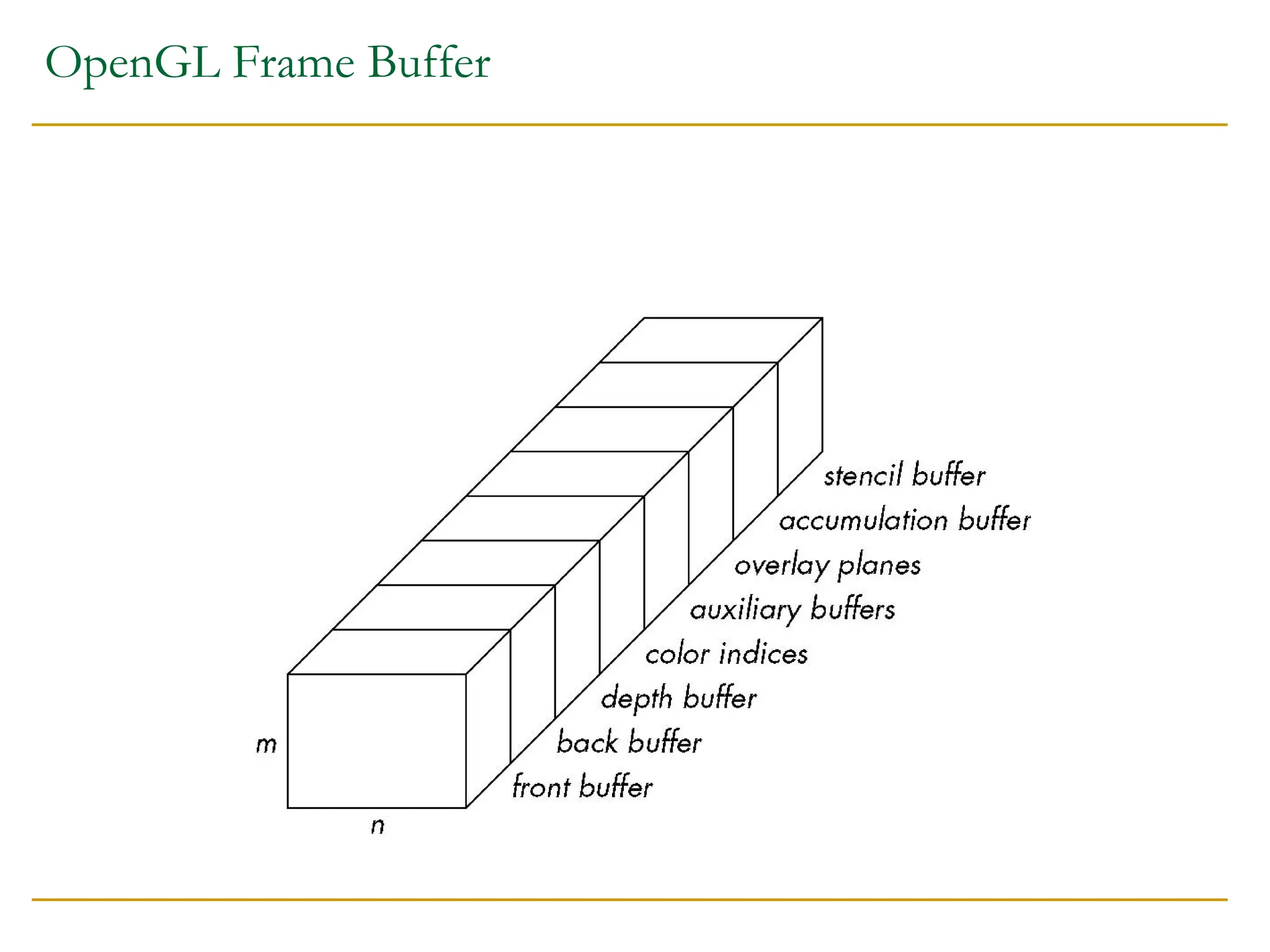
Buffer
Define a buffer by its spatial resolution (n x m) and its depth k, the
number of bits/pixel
pixel

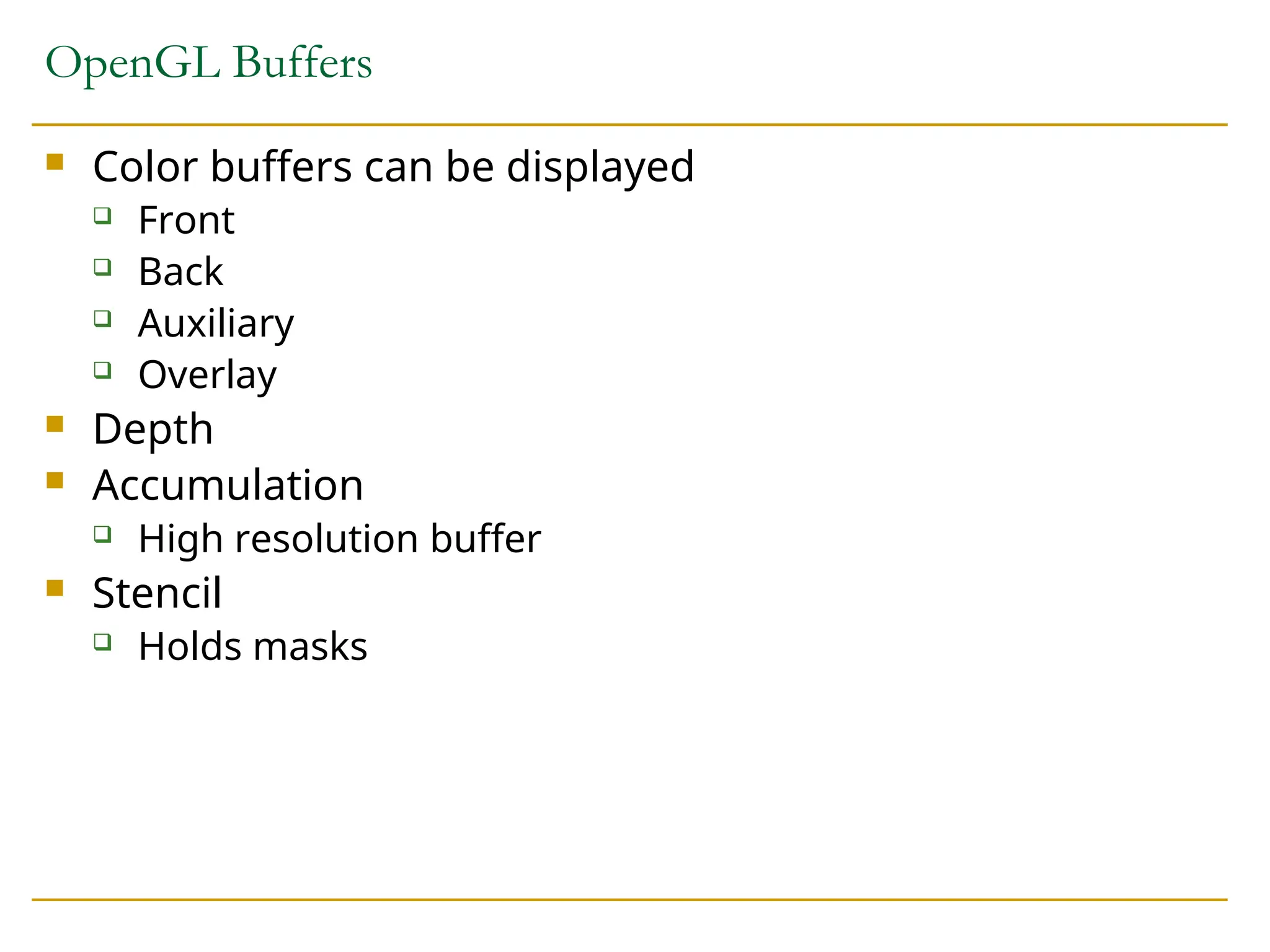
OpenGL Buffers
 Color buffers can be displayed
 Front
 Back
 Auxiliary
 Overlay
 Depth
 Accumulation
 High resolution buffer
 Stencil
 Holds masks

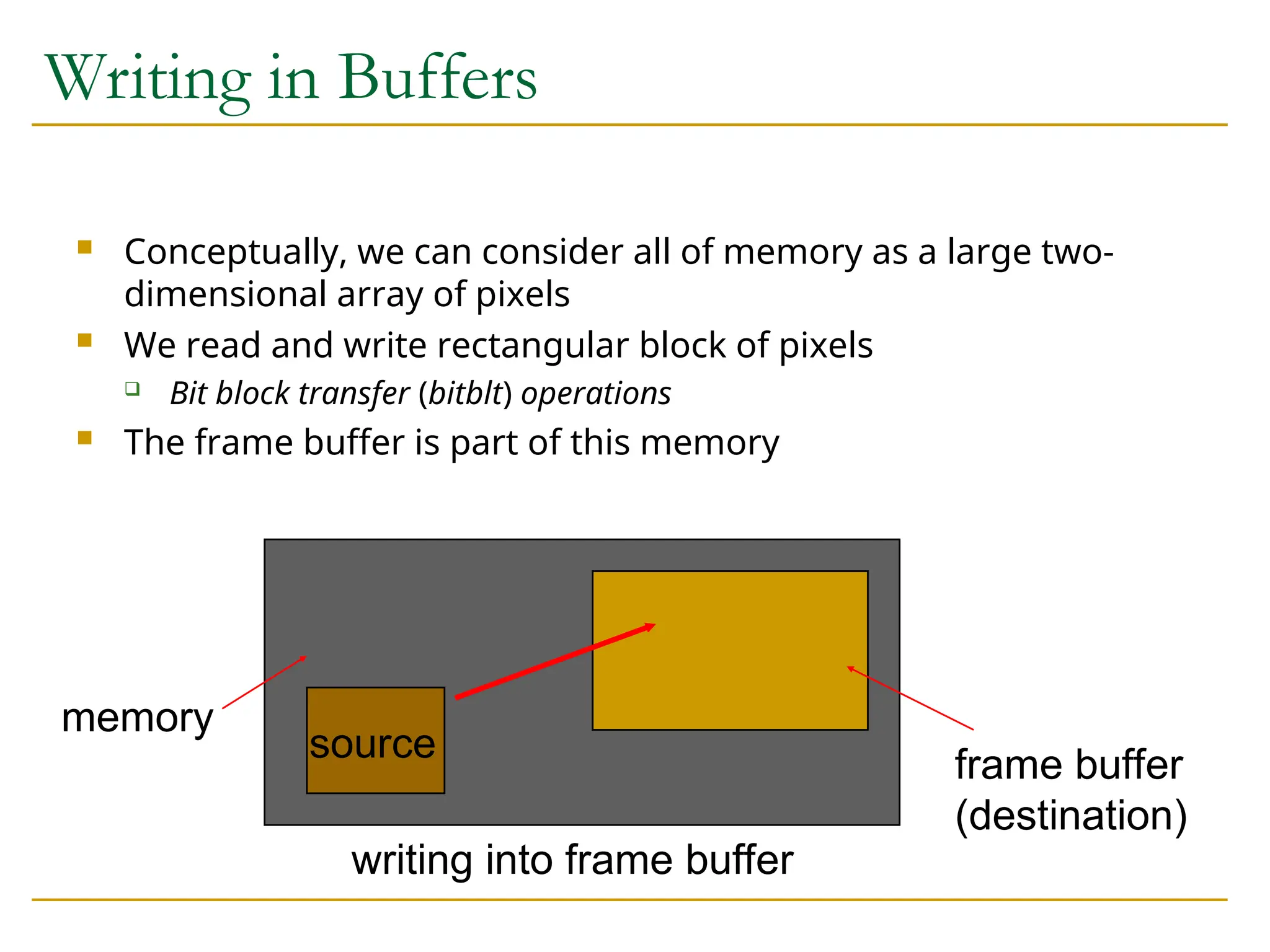
Writing in Buffers
 Conceptually, we can consider all of memory as a large two-
dimensional array of pixels
 We read and write rectangular block of pixels
 Bit block transfer (bitblt) operations
 The frame buffer is part of this memory
frame buffer
(destination)
writing into frame buffer
source
memory

Buffer Selection
 OpenGL can draw into or read from any of the color buffers
(front, back, auxiliary)
 Default to the back buffer

Change with glDrawBuffer and glReadBuffer
 Note that format of the pixels in the frame buffer is different
from that of processor memory and these two types of memory
reside in different places
 Need packing and unpacking
 Drawing and reading can be slow

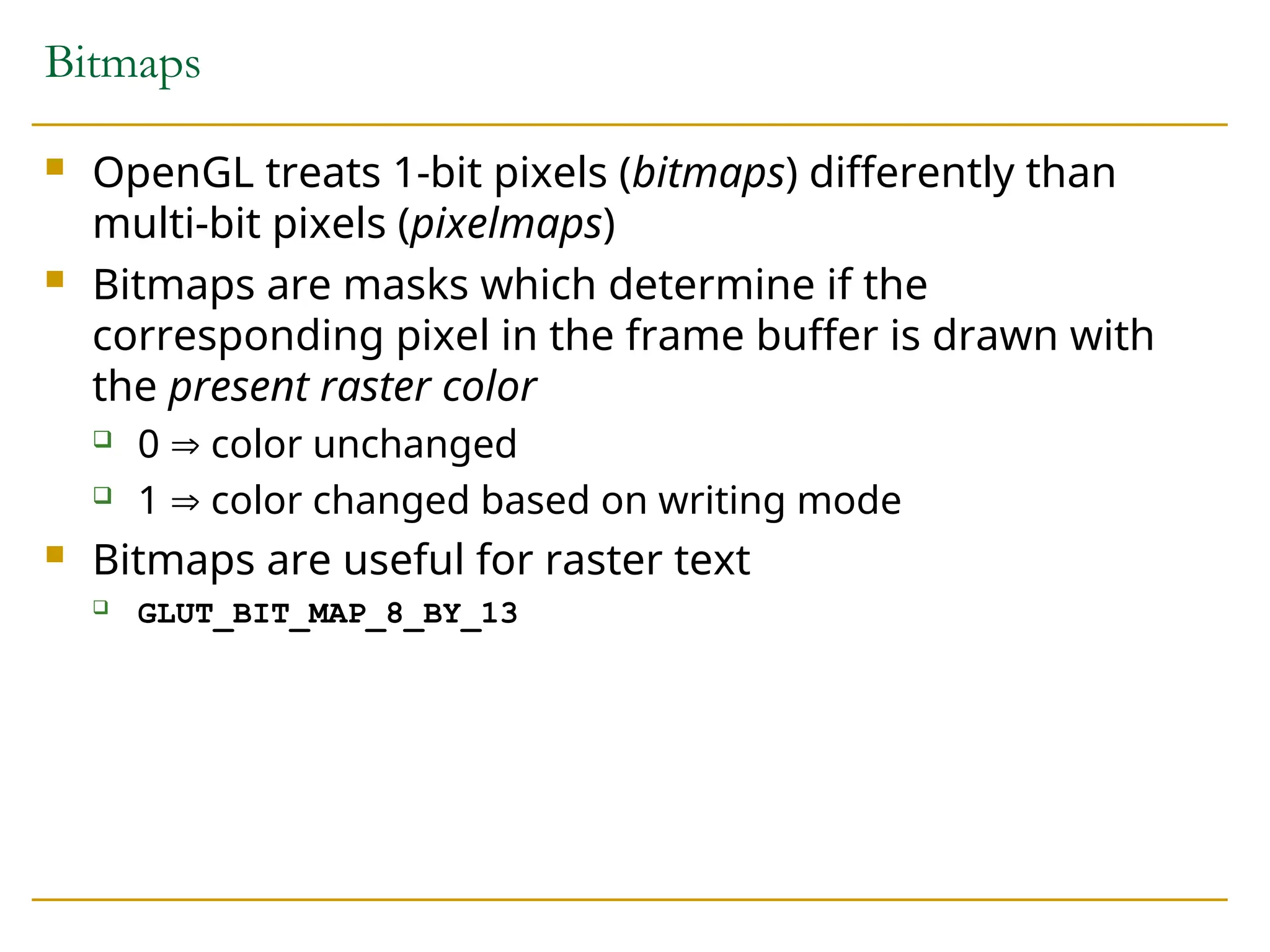
Bitmaps
 OpenGL treats 1-bit pixels (bitmaps) differently than
multi-bit pixels (pixelmaps)
 Bitmaps are masks which determine if the
corresponding pixel in the frame buffer is drawn with
the present raster color
 0  color unchanged
 1  color changed based on writing mode
 Bitmaps are useful for raster text
 GLUT_BIT_MAP_8_BY_13

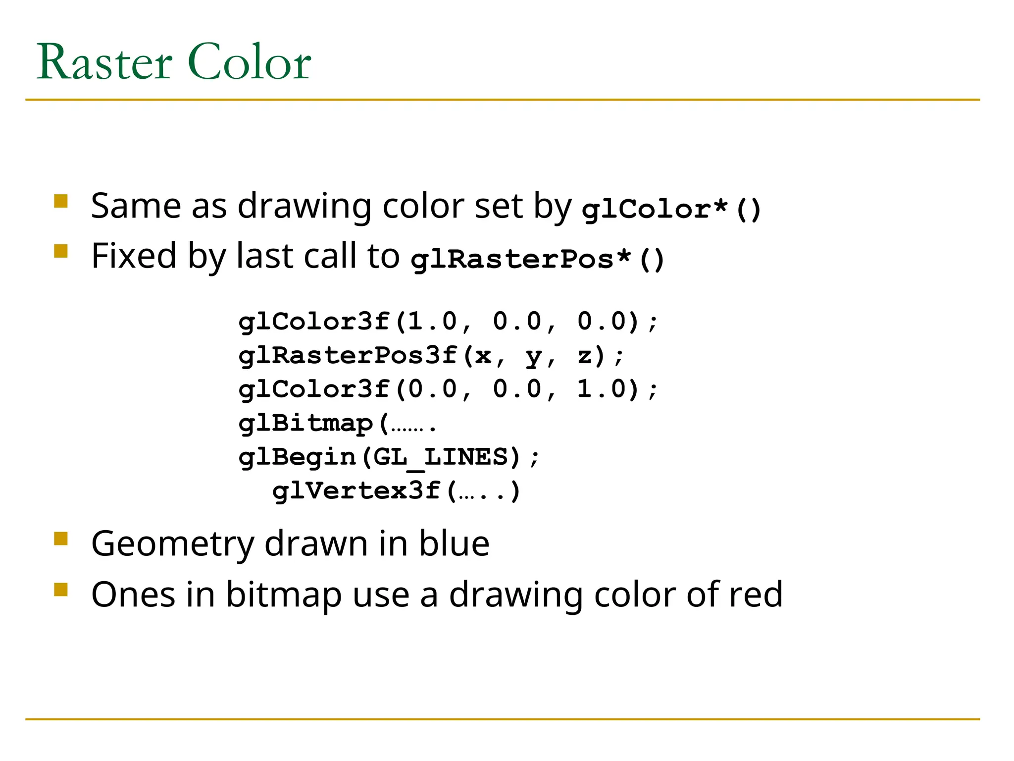
Raster Color
 Same as drawing color set by glColor*()
 Fixed by last call to glRasterPos*()
 Geometry drawn in blue
 Ones in bitmap use a drawing color of red
glColor3f(1.0, 0.0, 0.0);
glRasterPos3f(x, y, z);
glColor3f(0.0, 0.0, 1.0);
glBitmap(…….
glBegin(GL_LINES);
glVertex3f(…..)

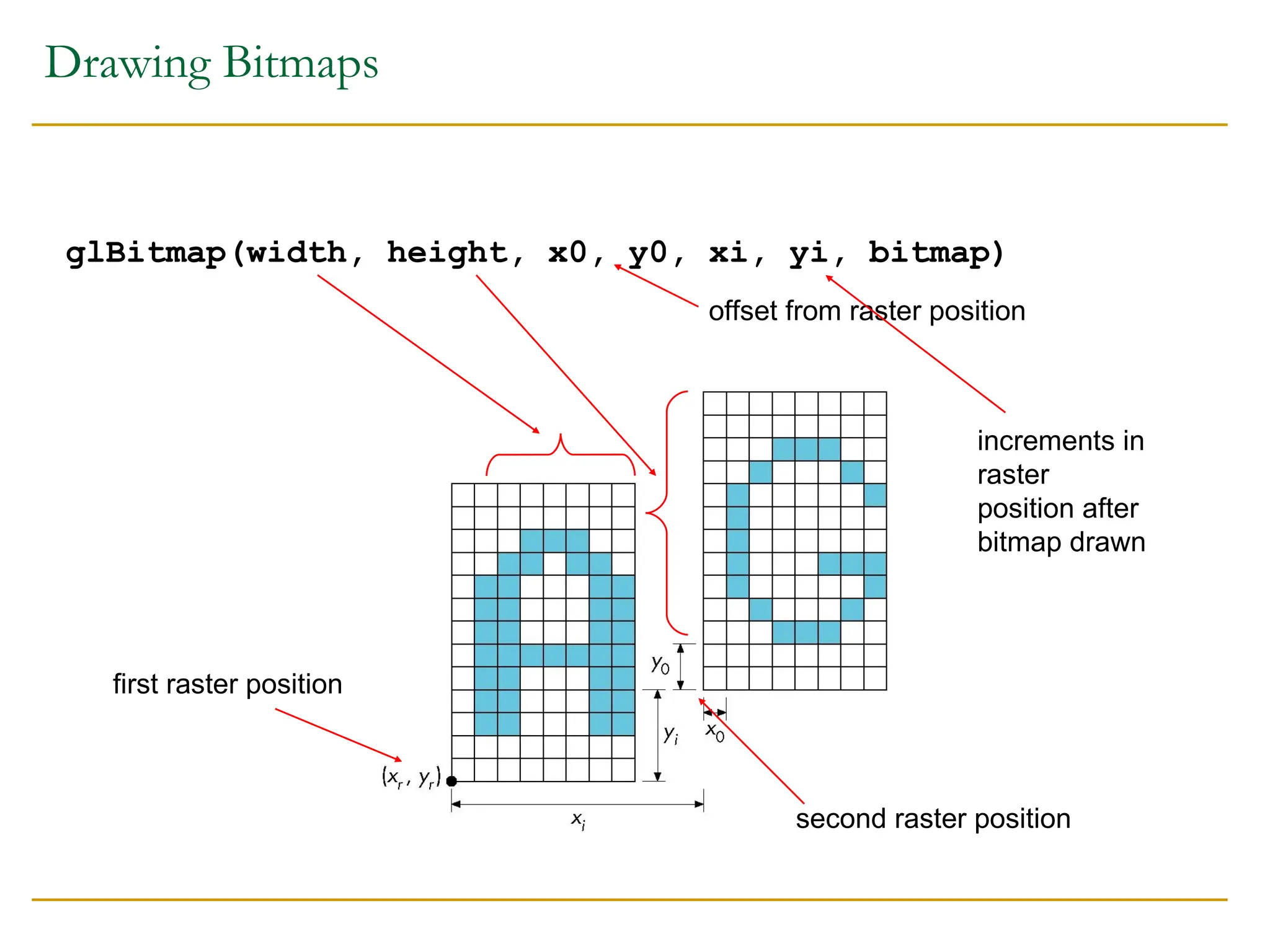
Drawing Bitmaps
glBitmap(width, height, x0, y0, xi, yi, bitmap)
first raster position
second raster position
offset from raster position
increments in
raster
position after
bitmap drawn

Example: Checker Board
GLubyte wb[2] = {0 x 00, 0 x ff};
GLubyte check[512];
int i, j;
for(j=0; i<64; i++) for (j=0; j<64, j++)
check[i*8+] = wb[(i/8+j)%2];
glBitmap( 64, 64, 0.0, 0.0, 0.0, 0.0, check);

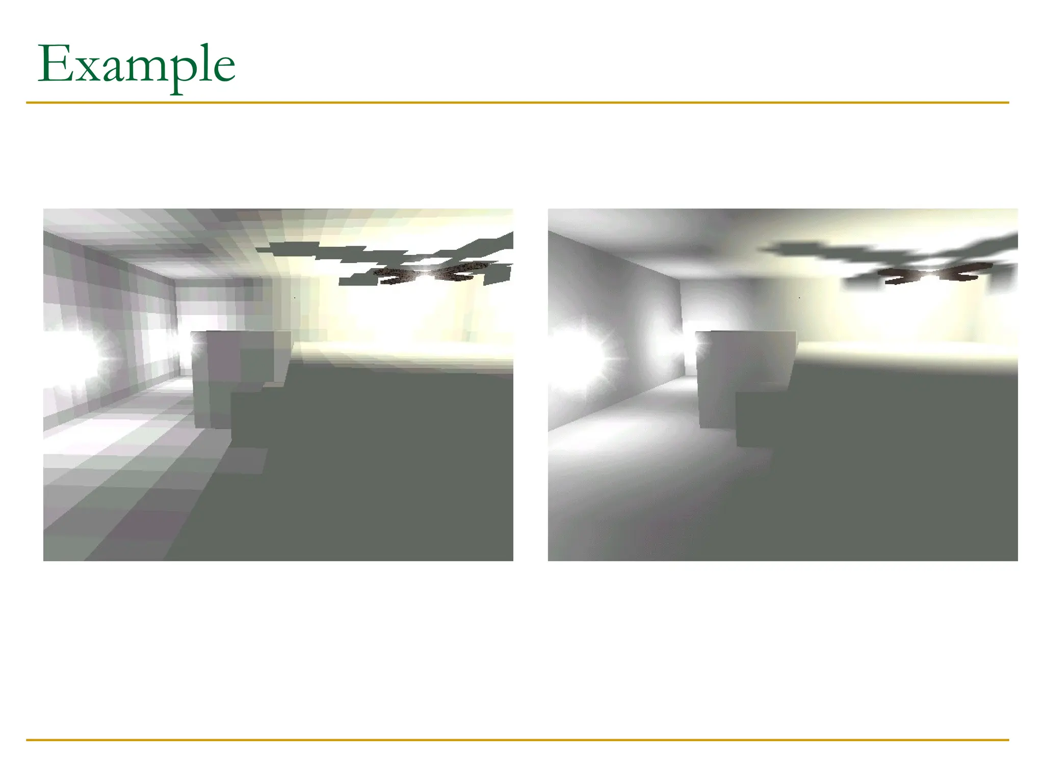
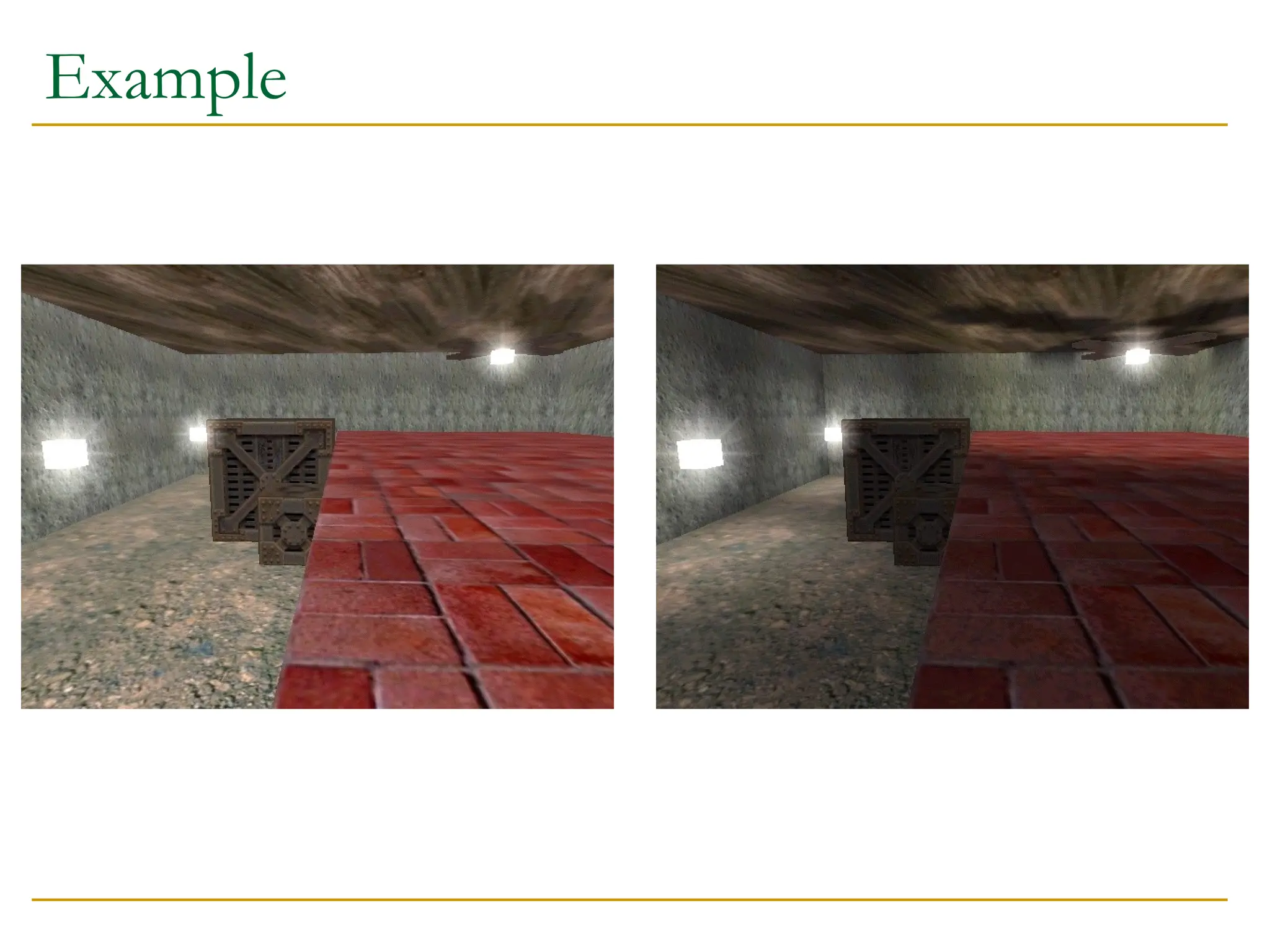
Light Maps
 Aim: Speed up lighting calculations by pre-computing
lighting and storing it in maps
 Allows complex illumination models to be used in
generating the map (eg shadows, radiosity)
 Used in complex rendering algorithms to catch radiance
(Radiance)
 Issues:
 How is the mapping determined?
 How are the maps generated?
 How are they applied at run-time?

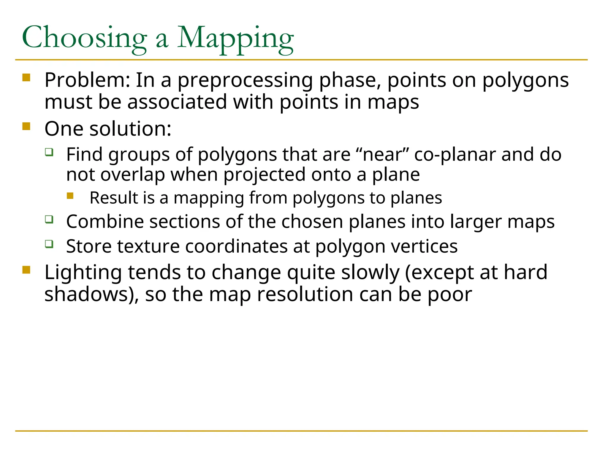
Choosing a Mapping
 Problem: In a preprocessing phase, points on polygons
must be associated with points in maps
 One solution:
 Find groups of polygons that are “near” co-planar and do
not overlap when projected onto a plane
 Result is a mapping from polygons to planes
 Combine sections of the chosen planes into larger maps
 Store texture coordinates at polygon vertices
 Lighting tends to change quite slowly (except at hard
shadows), so the map resolution can be poor

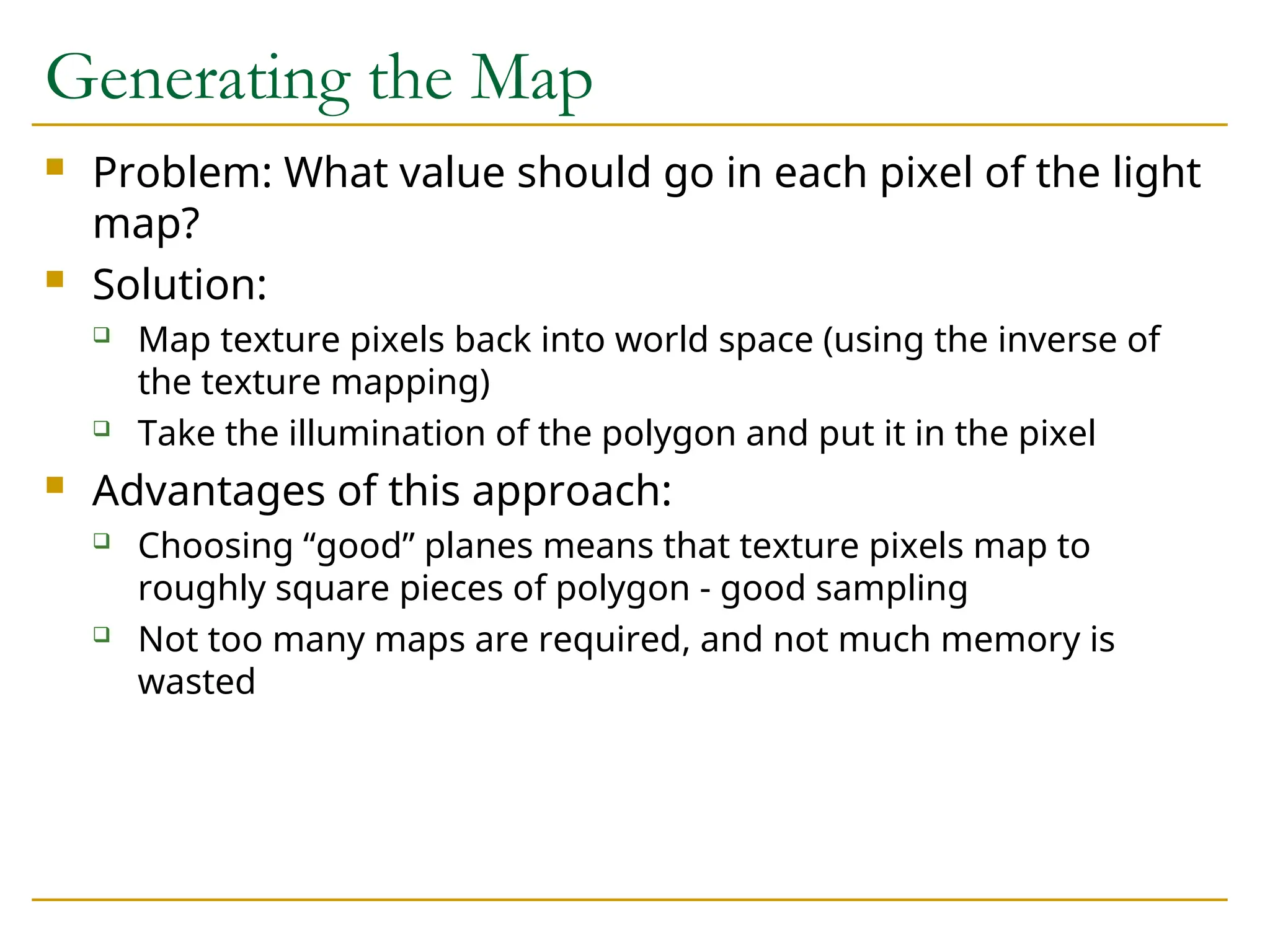
Generating the Map
 Problem: What value should go in each pixel of the light
map?
 Solution:
 Map texture pixels back into world space (using the inverse of
the texture mapping)
 Take the illumination of the polygon and put it in the pixel
 Advantages of this approach:
 Choosing “good” planes means that texture pixels map to
roughly square pieces of polygon - good sampling
 Not too many maps are required, and not much memory is
wasted

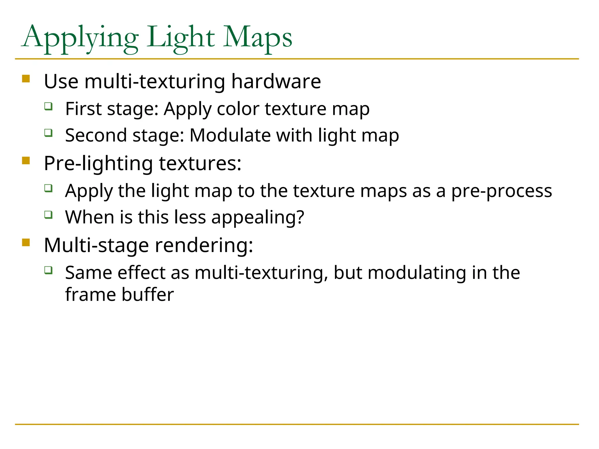
Applying Light Maps
 Use multi-texturing hardware
 First stage: Apply color texture map
 Second stage: Modulate with light map
 Pre-lighting textures:
 Apply the light map to the texture maps as a pre-process
 When is this less appealing?
 Multi-stage rendering:
 Same effect as multi-texturing, but modulating in the
frame buffer

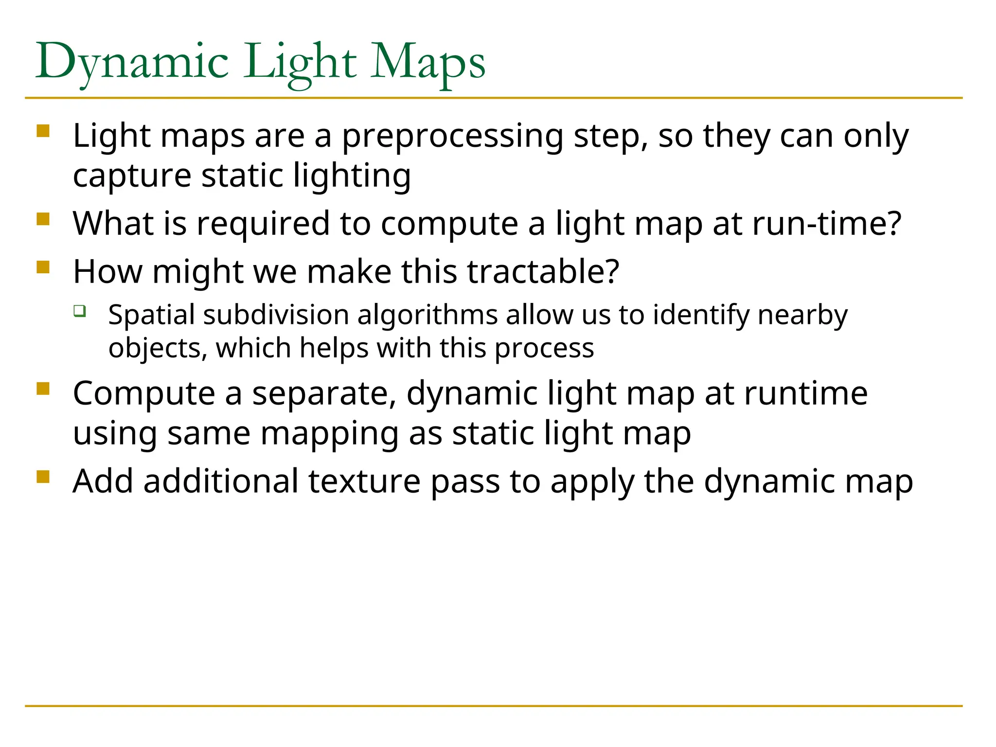
Dynamic Light Maps
 Light maps are a preprocessing step, so they can only
capture static lighting
 What is required to compute a light map at run-time?
 How might we make this tractable?
 Spatial subdivision algorithms allow us to identify nearby
objects, which helps with this process
 Compute a separate, dynamic light map at runtime
using same mapping as static light map
 Add additional texture pass to apply the dynamic map

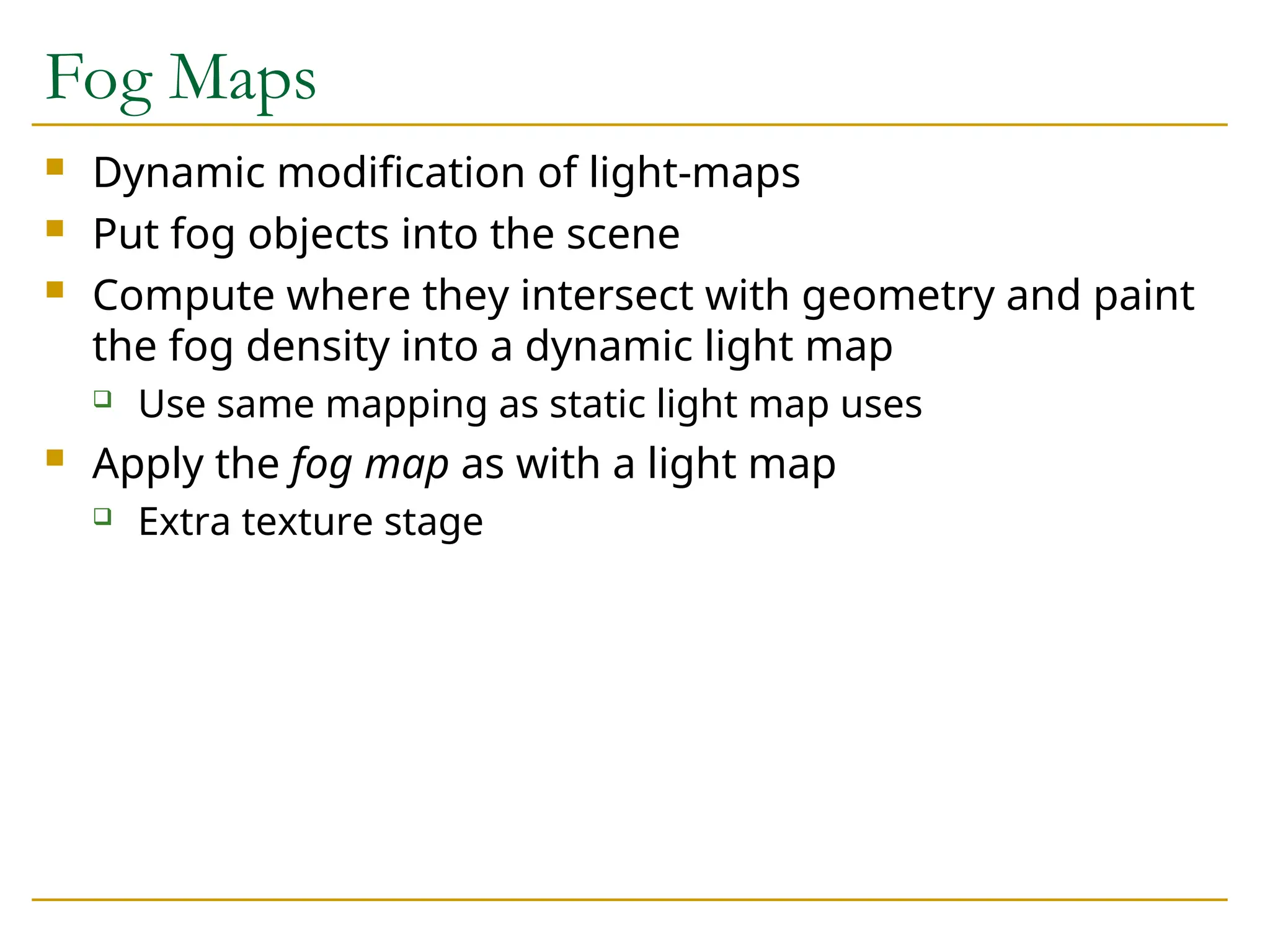
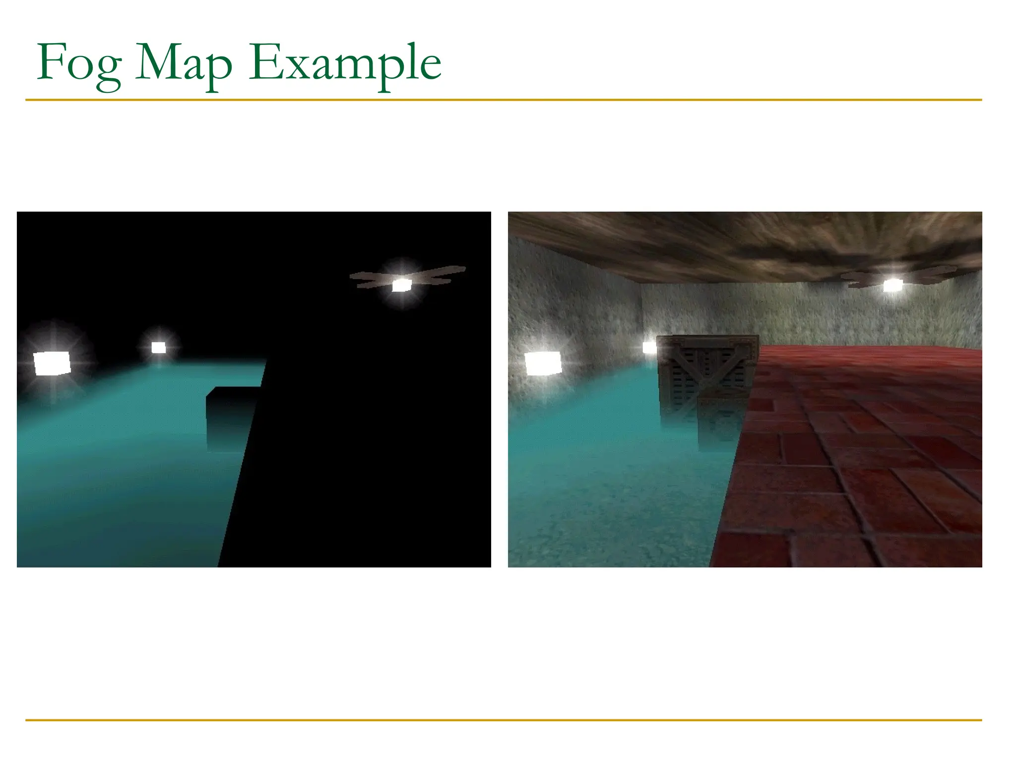
Fog Maps
 Dynamic modification of light-maps
 Put fog objects into the scene
 Compute where they intersect with geometry and paint
the fog density into a dynamic light map
 Use same mapping as static light map uses
 Apply the fog map as with a light map
 Extra texture stage

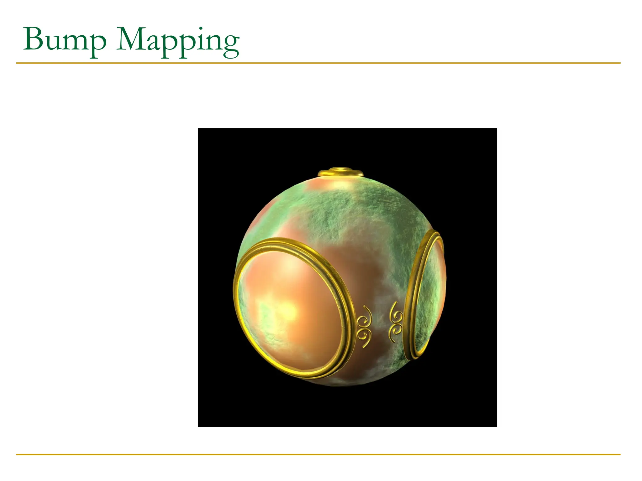
Bump Mapping
 Bump mapping modifies the surface normal vector
according to information in the map
 View dependent: the effect of the bumps depends on
which direction the surface is viewed from
 Bump mapping can be implemented with multi-
texturing or multi-pass rendering

Storing the Bump Map
 Several options for what to store in the map
 The normal vector to use
 An offset to the default normal vector
 Data derived from the normal vector
 Illumination changes for a fixed view
 Multi-texturing map:
 Store four maps (or more) showing the illumination effects
of the bumps from four (or more) view directions
 Key point: Bump maps on diffuse surfaces just make them
lighter or darker - don’t change the color

Multi-Texture Bump Maps
 At run time:
 Compute the dot product of the view direction with the ideal
view direction for each bump map
 Bump maps that were computed with views near the current one
will have big dot products
 Use the computed dot product as a blend factor when applying
each bump map
 Must be able to specify the blend function to the texture unit
 OpenGL allows this
 Textbook has details for more accurate bump-mapping
 Note that computing a dot product between the light and the
bump map value can be done with current hardware

Multi-Pass Rendering
 The pipeline takes one triangle at a time, so only local
information, and pre-computed maps, are available
 Multi-Pass techniques render the scene, or parts of the
scene, multiple times
 Makes use of auxiliary buffers to hold information
 Make use of tests and logical operations on values in the buffers
 Really, a set of functionality that can be used to achieve a wide
range of effects
 Mirrors, shadows, bump-maps, anti-aliasing, compositing, …

Buffers
 Color buffers: Store RGBA color information for each
pixel
 OpenGL actually defines four or more color buffers: front/back,
left/right and auxiliary color buffers
 Depth buffer: Stores depth information for each pixel
 Stencil buffer: Stores some number of bits for each pixel
 Accumulation buffer: Like a color buffer, but with higher
resolution and different operations
 Buffers are defined by:
 The type of values they store
 The logical operations that they influence
 The way they are written and read

Fragment Tests
 A fragment is a pixel-sized piece of shaded polygon,
with color and depth information
 The tests and operations performed with the fragment
on its way to the color buffer are essential to
understanding multi-pass techniques
 Most important are, in order:
 Alpha test
 Stencil test
 Depth test
 Blending
 As the fragment passes through, some of the buffers
may also have values stored into them

Alpha Test
 The alpha test either allows a fragment to pass, or stops
it, depending on the outcome of a test:
 Here, fragment is the fragment’s alpha value, and reference is
a reference alpha value that you specify
 op is one of:
 <, <=, =, !=, >, >=
 There are also the special tests: Always and Never
 Always let the fragment through or never let it through
 What is a sensible default?
if ( fragment op reference )
pass fragment on

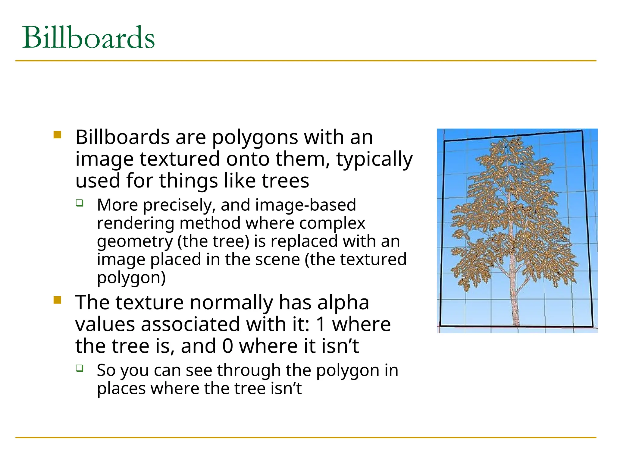
Billboards
 Billboards are polygons with an
image textured onto them, typically
used for things like trees
 More precisely, and image-based
rendering method where complex
geometry (the tree) is replaced with an
image placed in the scene (the textured
polygon)
 The texture normally has alpha
values associated with it: 1 where
the tree is, and 0 where it isn’t
 So you can see through the polygon in
places where the tree isn’t

Alpha Test and Billboards
 You can use texture blending to make the polygon see
through, but there is a big problem
 What happens if you draw the billboard and then draw
something behind it?
 Hint: Think about the depth buffer values
 This is one reason why transparent objects must be rendered
back to front
 The best way to draw billboards is with an alpha test: Do
not let alpha < 0.5 pass through
 Depth buffer is never set for fragments that are see through
 Doesn’t work for transparent polygons - more later

Stencil Buffer
 The stencil buffer acts like a paint stencil - it lets some
fragments through but not others
 It stores multi-bit values
 You specify two things:
 The test that controls which fragments get through
 The operations to perform on the buffer when the test passes or
fails
 All tests/operation look at the value in the stencil that
corresponds to the pixel location of the fragment
 Typical usage: One rendering pass sets values in the
stencil, which control how various parts of the screen
are drawn in the second pass

Multi-Pass Algorithms
 Designing a multi-pass algorithm is a non-trivial task
 At least one person I know of has received a PhD for developing
such algorithms
 References for multi-pass algorithms:
 The OpenGL Programming guide discusses many multi-pass
techniques in a reasonably understandable manner
 Game Programming Gems has some
 Watt and Policarpo has others
 Several have been published as academic papers
 As always, the web is your friend

Planar Reflections (Flat Mirrors)
 Use the stencil buffer, color buffer and depth
buffer
 Basic idea:
 We need to draw all the stuff around the mirror
 We need to draw the stuff in the mirror, reflected,
without drawing over the things around the mirror
 Key point: You can reflect the viewpoint about the
mirror to see what is seen in the mirror, or you can
reflect the world about the mirror

Rendering Reflected First
 First pass:
 Render the reflected scene without mirror, depth test on
 Second pass:
 Disable the color buffer, Enable the stencil buffer to always pass
but set the buffer, Render the mirror polygon
 Now, set the stencil test to only pass points outside the mirror
 Clear the color buffer - does not clear points inside mirror area
 Third Pass:
 Enable the color buffer again, Disable the stencil buffer
 Render the original scene, without the mirror
 Depth buffer stops from writing over things in mirror

Reflected Scene First (issues)
 If the mirror is infinite, there is no need for the second
pass
 But might want to apply a texture to roughen the reflection
 If the mirror plane is covered in something (a wall) then
no need to use the stencil or clear the color buffer in
pass 2
 Objects behind the mirror cause problems:
 Will appear in reflected view in front of mirror
 Solution is to use clipping plane to cut away things on wrong
side of mirror
 Curved mirrors by reflecting vertices differently
 Doesn’t do:
 Reflections of mirrors in mirrors (recursive reflections)
 Multiple mirrors in one scene (that aren’t seen in each other)

Rendering Normal First
 First pass:
 Render the scene without the mirror
 Second pass:
 Clear the stencil, Render the mirror, setting the stencil if
the depth test passes
 Third pass:
 Clear the depth buffer with the stencil active, passing
things inside the mirror only
 Reflect the world and draw using the stencil test. Only
things seen in the mirror will be drawn

Normal First Addendum
 Same problem with objects behind mirror
 Same solution
 Can manage multiple mirrors
 Render normal view, then do other passes for each mirror
 Only works for non-overlapping mirrors (in view)
 But, could be extended with more tests and passes
 A recursive formulation exists for mirrors that see other
mirrors

The Limits of Geometric Modeling
 Although graphics cards can render over 10 million
polygons per second, that number is insufficient
for many phenomena
 Clouds
 Grass
 Terrain
 Skin

Modeling an Orange
 Consider the problem of modeling an orange (the
fruit)
 Start with an orange-colored sphere
 Too simple
 Replace sphere with a more complex shape
 Does not capture surface characteristics (small
dimples)
 Takes too many polygons to model all the dimples

Modeling an Orange (cont.)
 Take a picture of a real orange, scan it, and “paste” onto
simple geometric model
 This process is texture mapping
 Still might not be sufficient because resulting surface
will be smooth
 Need to change local shape
 Bump mapping

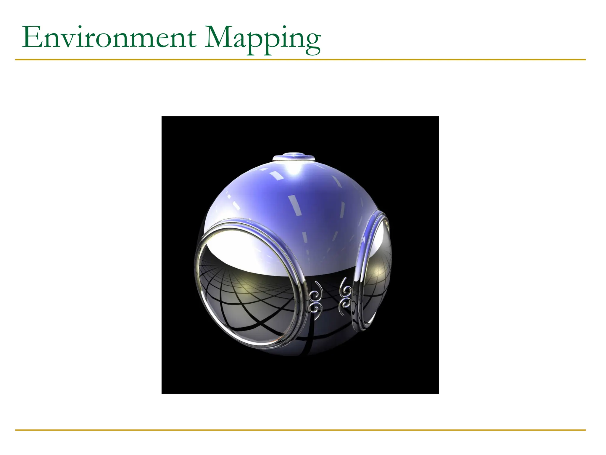
Three Types of Mapping
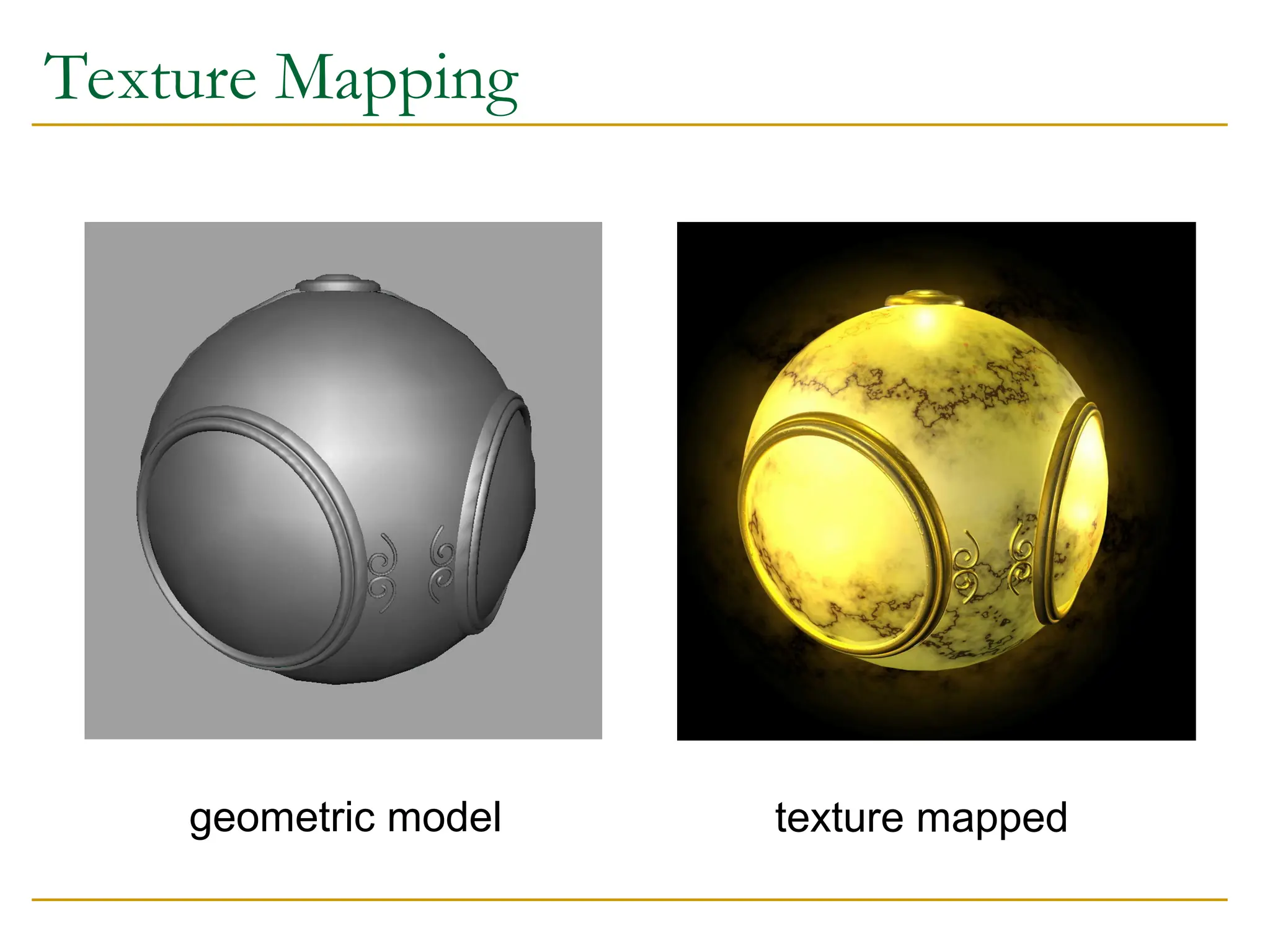
 Texture Mapping
 Uses images to fill inside of polygons
 Environmental (reflection mapping)
 Uses a picture of the environment for texture maps
 Allows simulation of highly specular surfaces
 Bump mapping
 Emulates altering normal vectors during the rendering
process

Texture Mapping
geometric model texture mapped

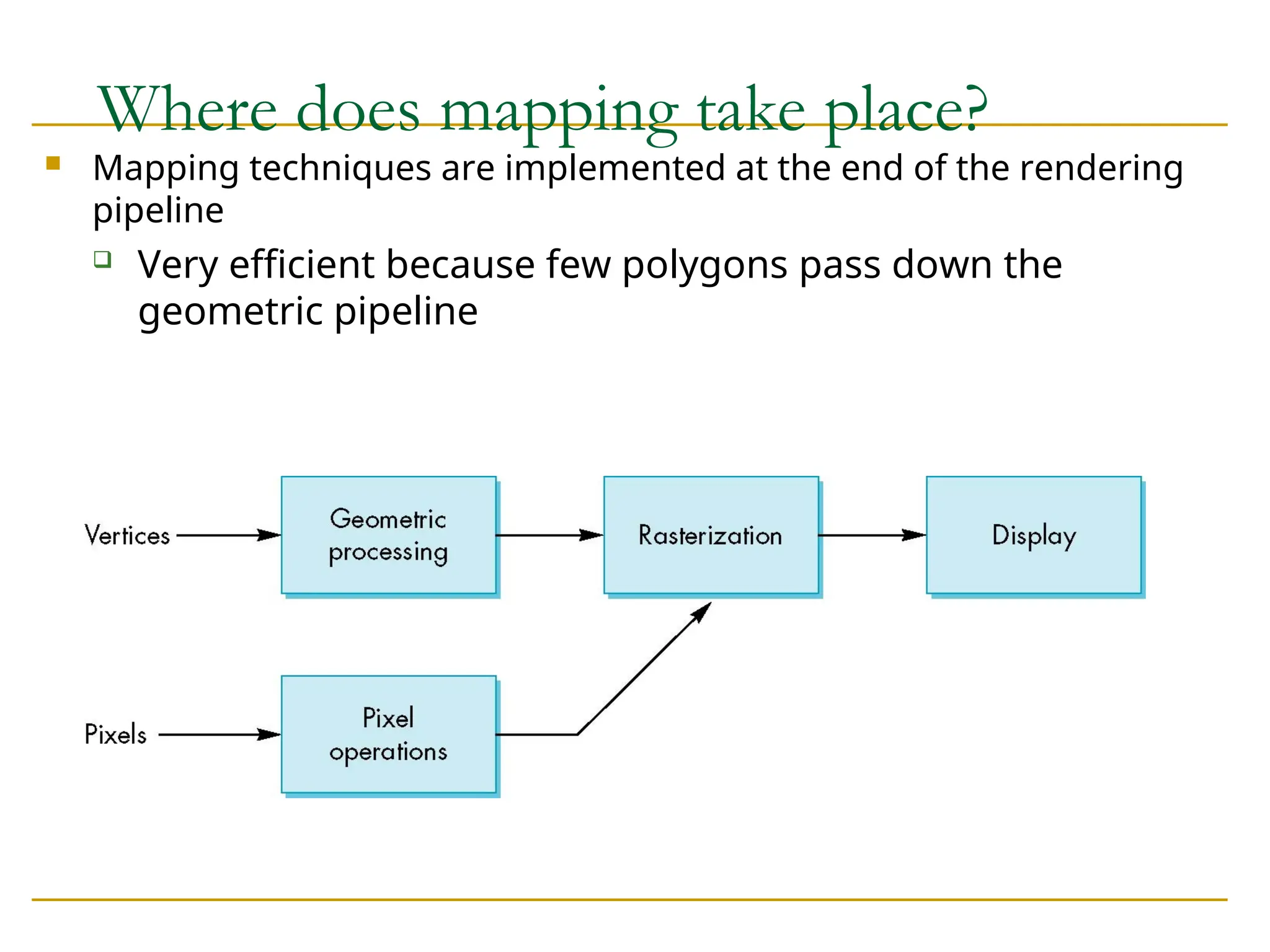
Where does mapping take place?
 Mapping techniques are implemented at the end of the rendering
pipeline
 Very efficient because few polygons pass down the
geometric pipeline

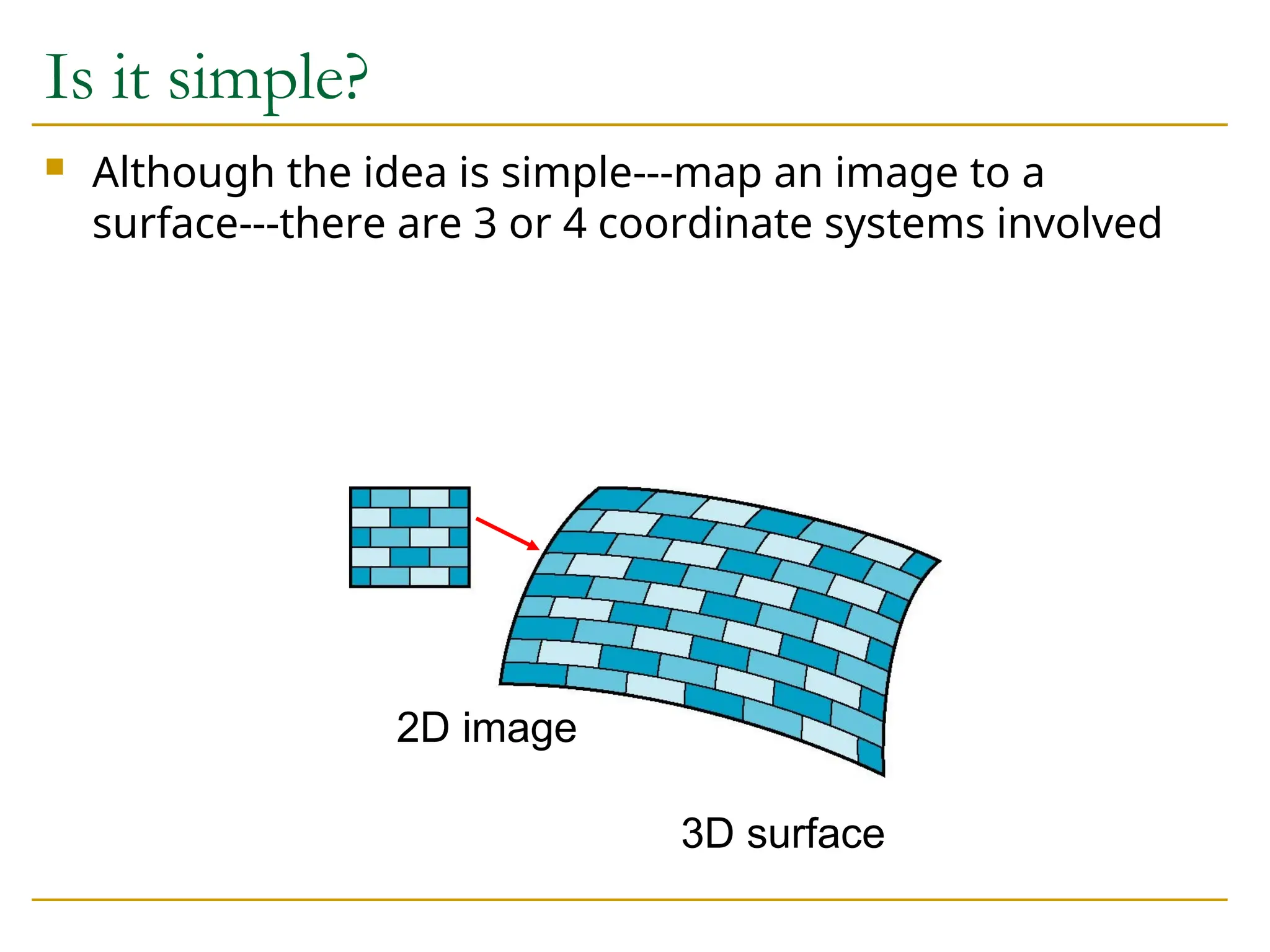
Is it simple?
 Although the idea is simple---map an image to a
surface---there are 3 or 4 coordinate systems involved
2D image
3D surface

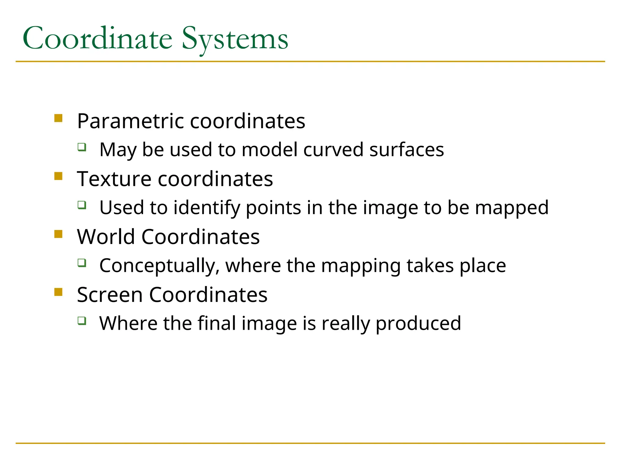
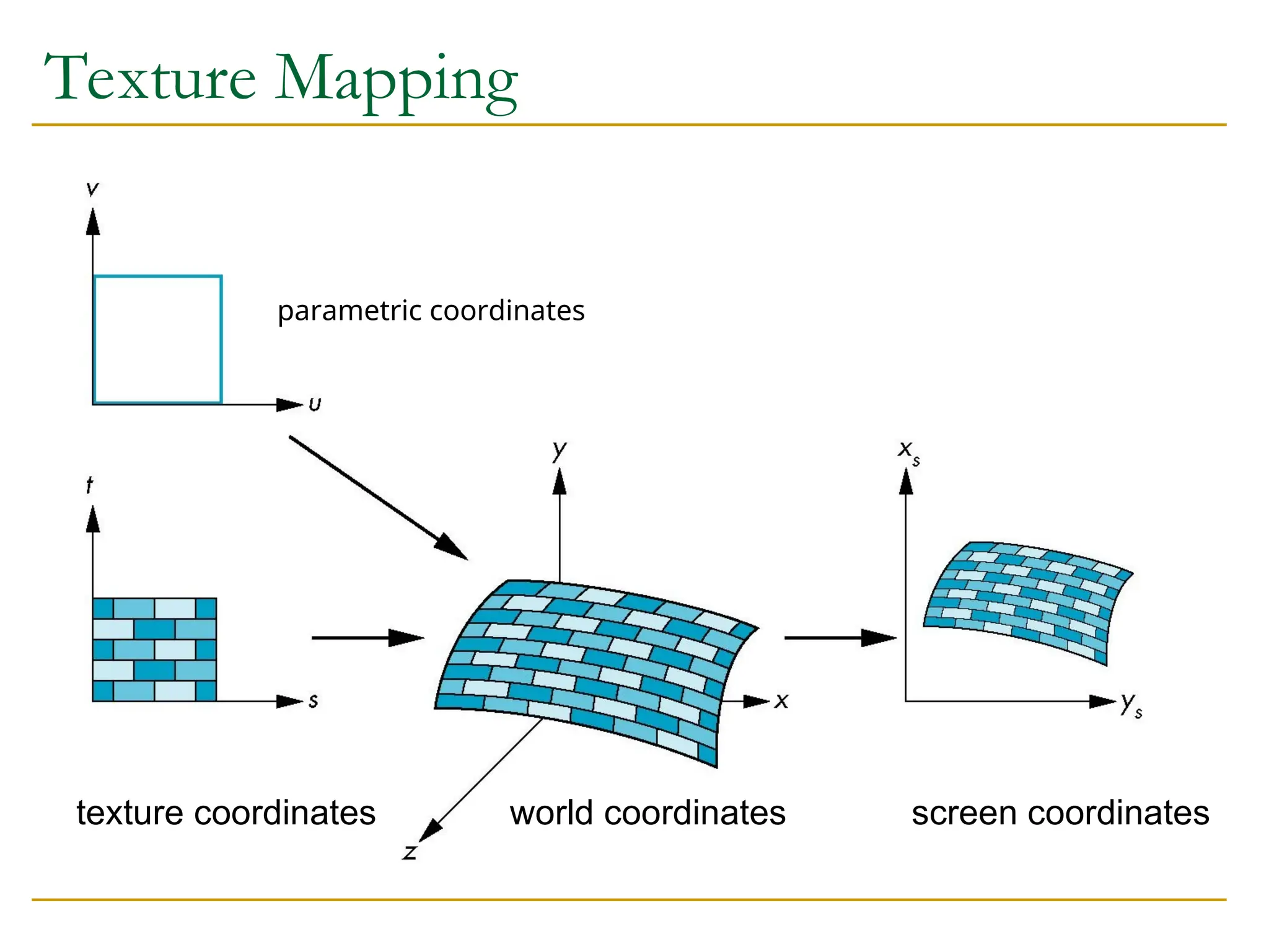
Coordinate Systems
 Parametric coordinates
 May be used to model curved surfaces
 Texture coordinates
 Used to identify points in the image to be mapped
 World Coordinates
 Conceptually, where the mapping takes place
 Screen Coordinates
 Where the final image is really produced

Texture Mapping
parametric coordinates
texture coordinates world coordinates screen coordinates

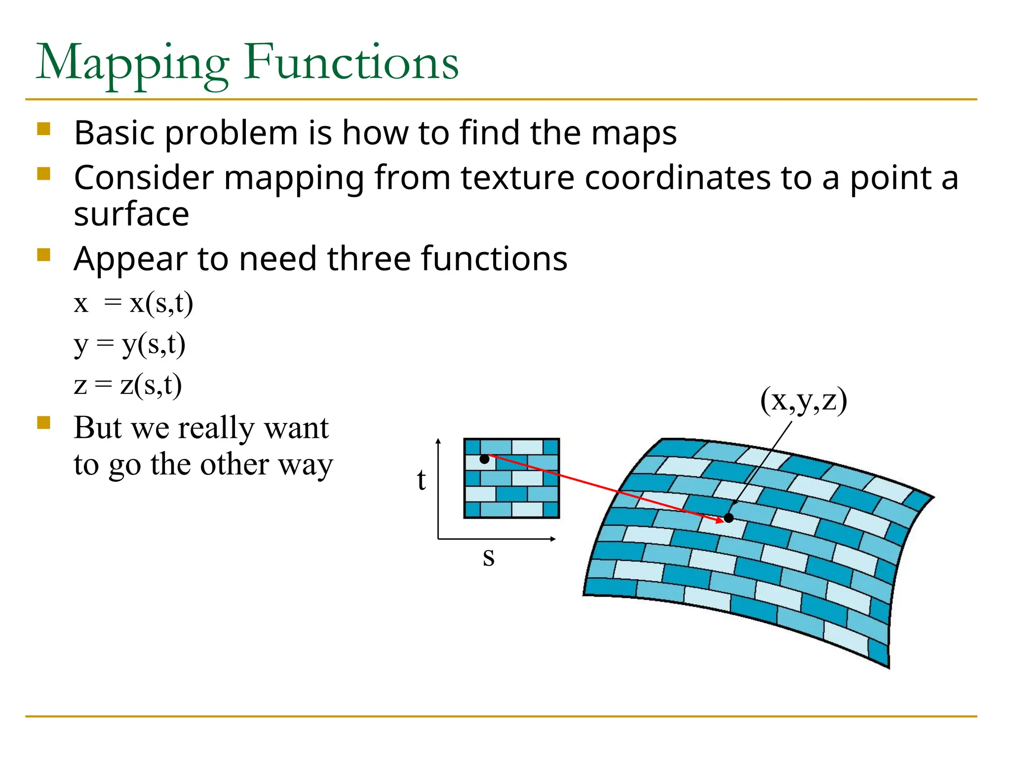
Mapping Functions
 Basic problem is how to find the maps
 Consider mapping from texture coordinates to a point a
surface
 Appear to need three functions
x = x(s,t)
y = y(s,t)
z = z(s,t)
 But we really want
to go the other way
s
t
(x,y,z)

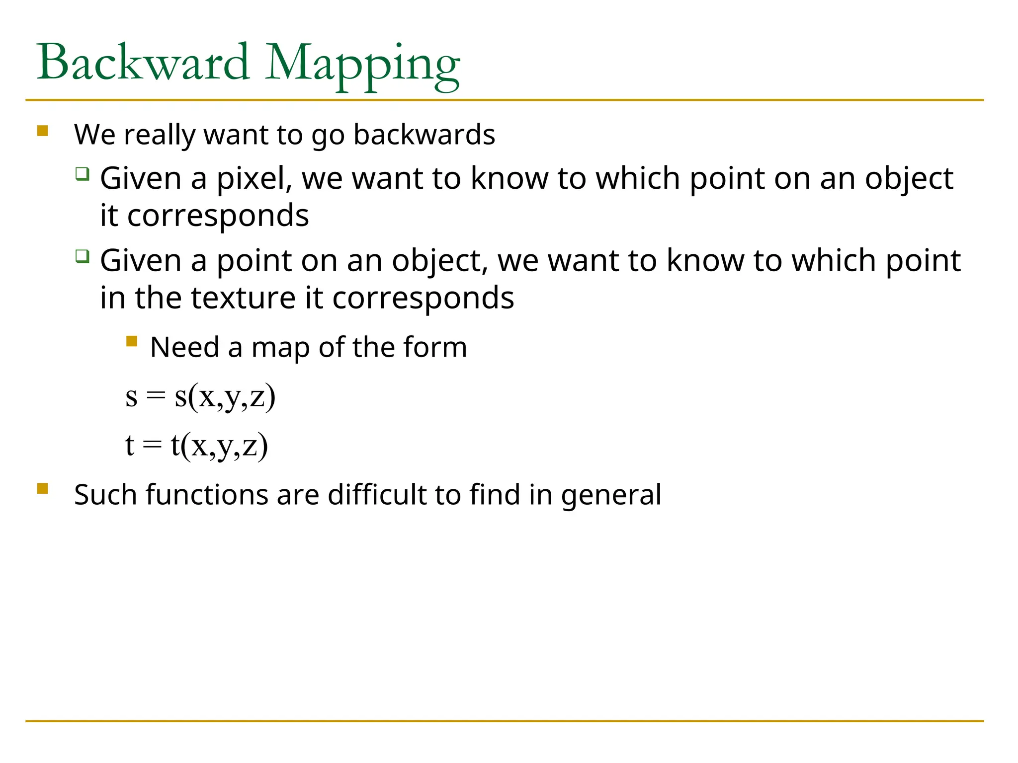
Backward Mapping
 We really want to go backwards
 Given a pixel, we want to know to which point on an object
it corresponds
 Given a point on an object, we want to know to which point
in the texture it corresponds

Need a map of the form
s = s(x,y,z)
t = t(x,y,z)

Such functions are difficult to find in general

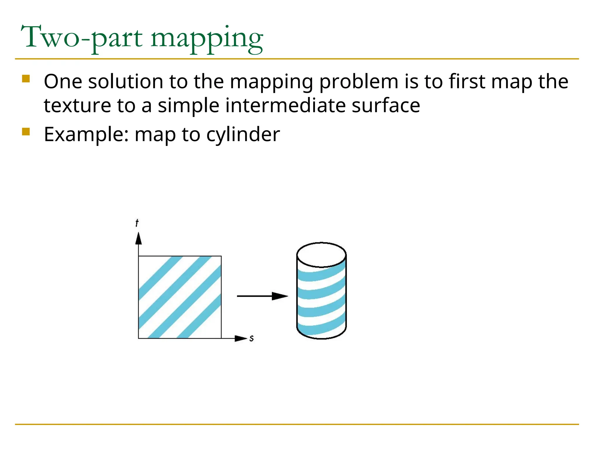
Two-part mapping
 One solution to the mapping problem is to first map the
texture to a simple intermediate surface
 Example: map to cylinder

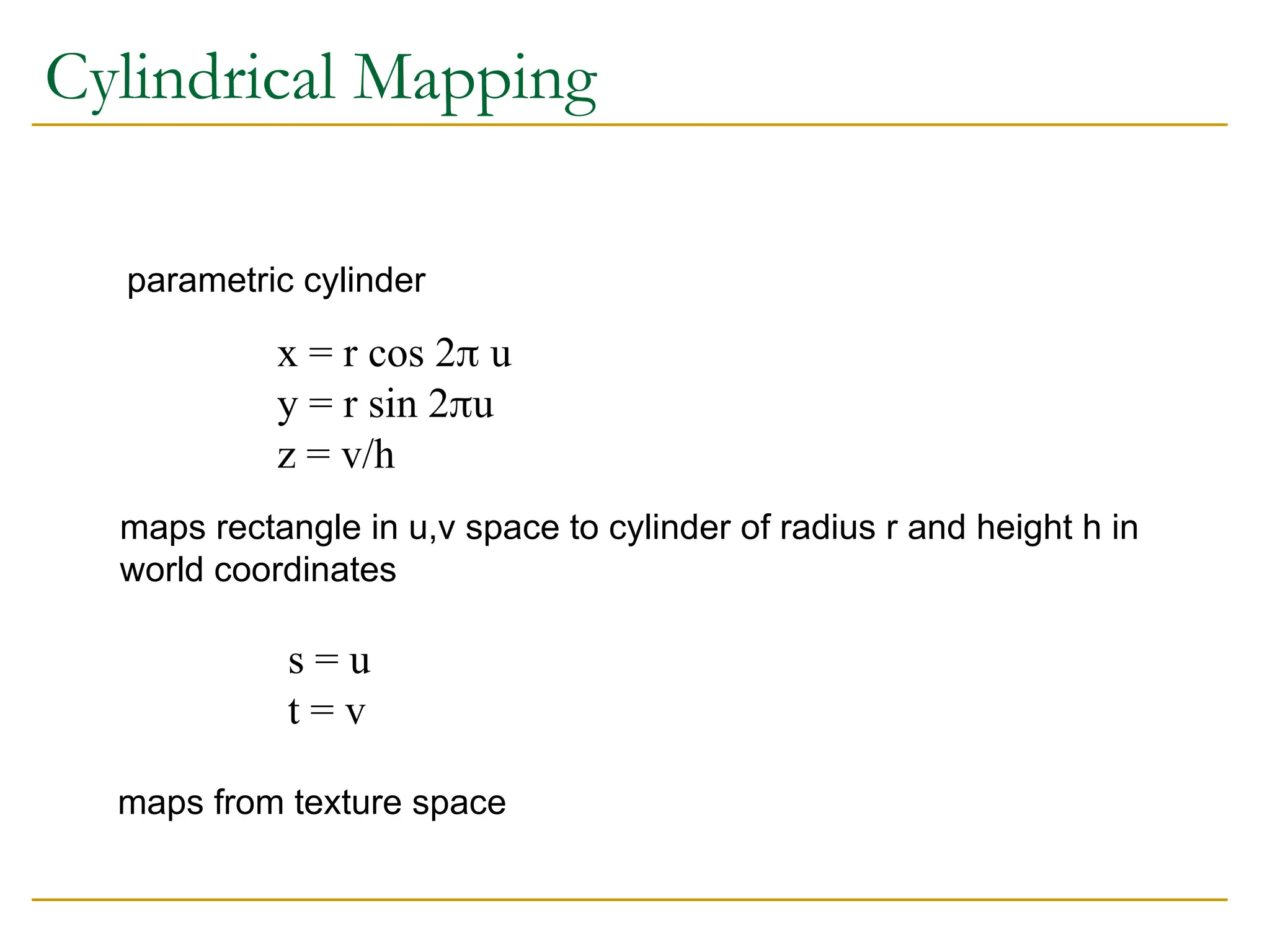
Cylindrical Mapping
parametric cylinder
x = r cos 2 u
y = r sin 2u
z = v/h
maps rectangle in u,v space to cylinder of radius r and height h in
world coordinates
s = u
t = v
maps from texture space

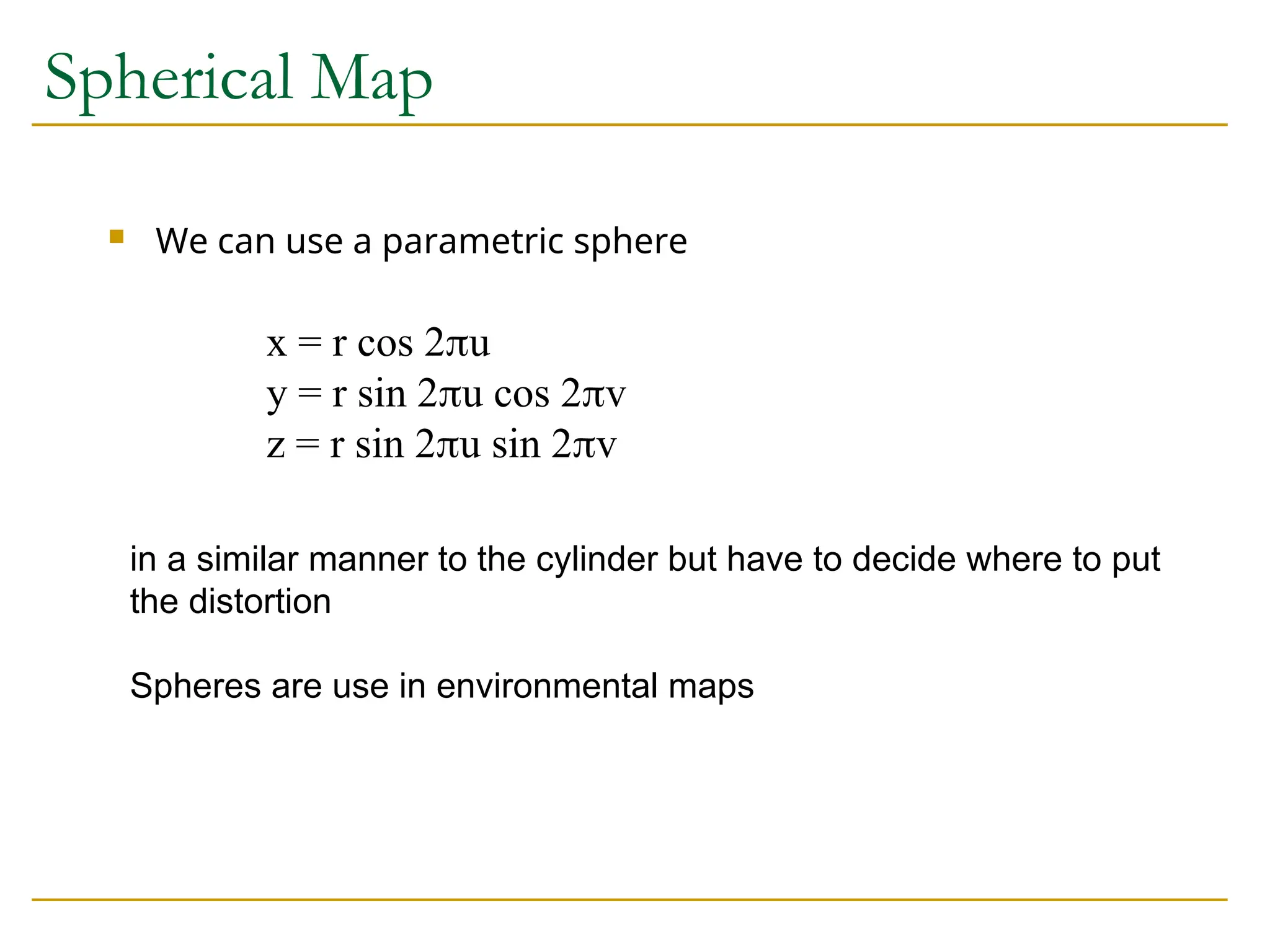
Spherical Map
 We can use a parametric sphere
x = r cos 2u
y = r sin 2u cos 2v
z = r sin 2u sin 2v
in a similar manner to the cylinder but have to decide where to put
the distortion
Spheres are use in environmental maps

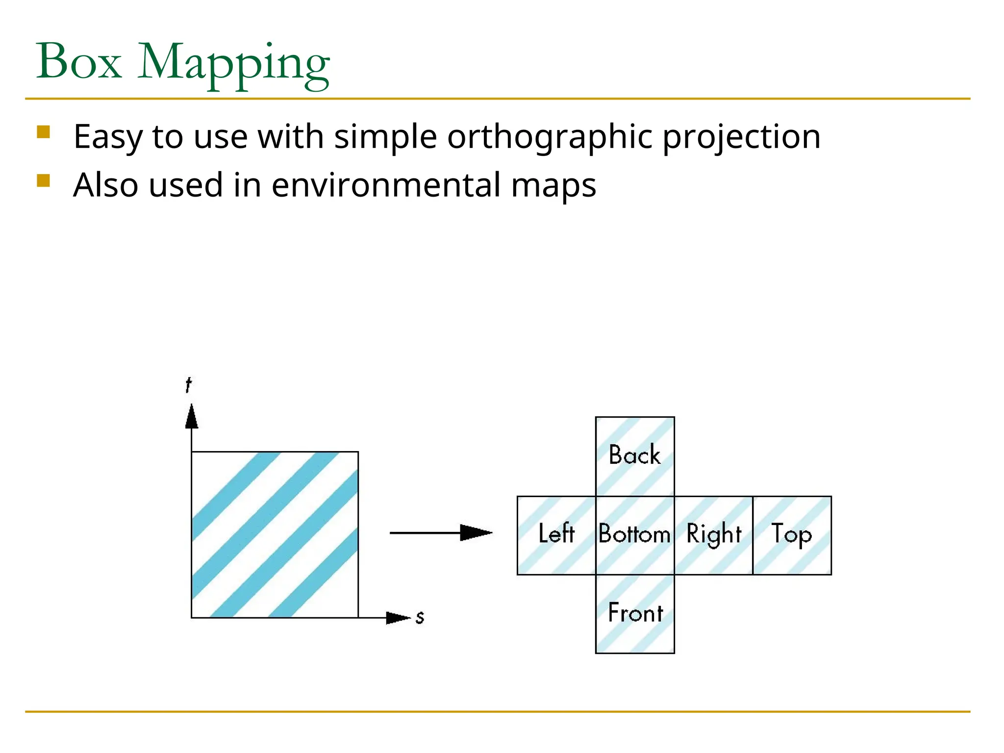
Box Mapping
 Easy to use with simple orthographic projection
 Also used in environmental maps

Second Mapping
 Map from intermediate object to actual object
 Normals from intermediate to actual
 Normals from actual to intermediate
 Vectors from center of intermediate
intermediate
actual

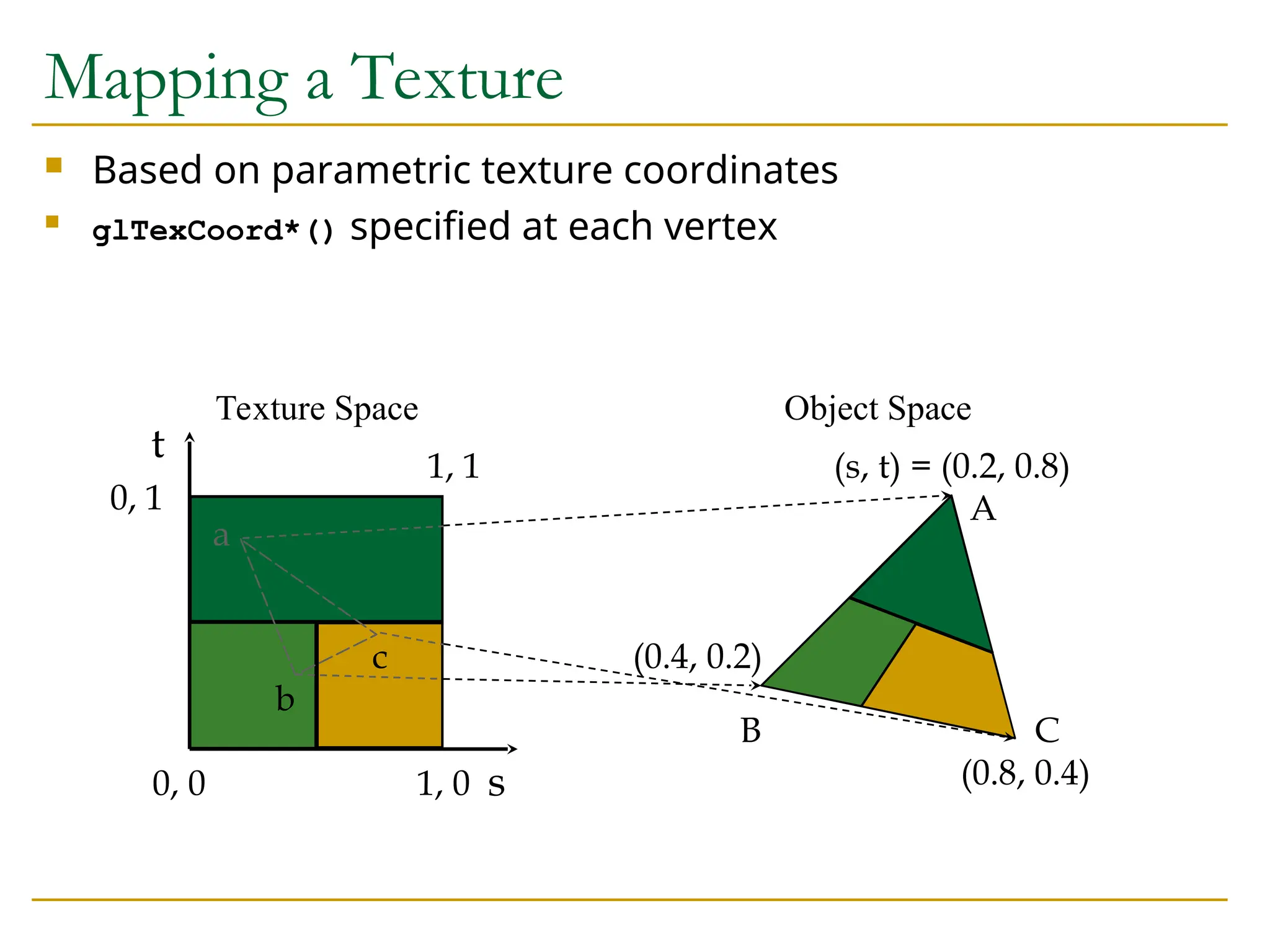
 Based on parametric texture coordinates

glTexCoord*() specified at each vertex
s
t 1, 1
0, 1
0, 0 1, 0
(s, t) = (0.2, 0.8)
(0.4, 0.2)
(0.8, 0.4)
A
B C
a
b
c
Texture Space Object Space
Mapping a Texture

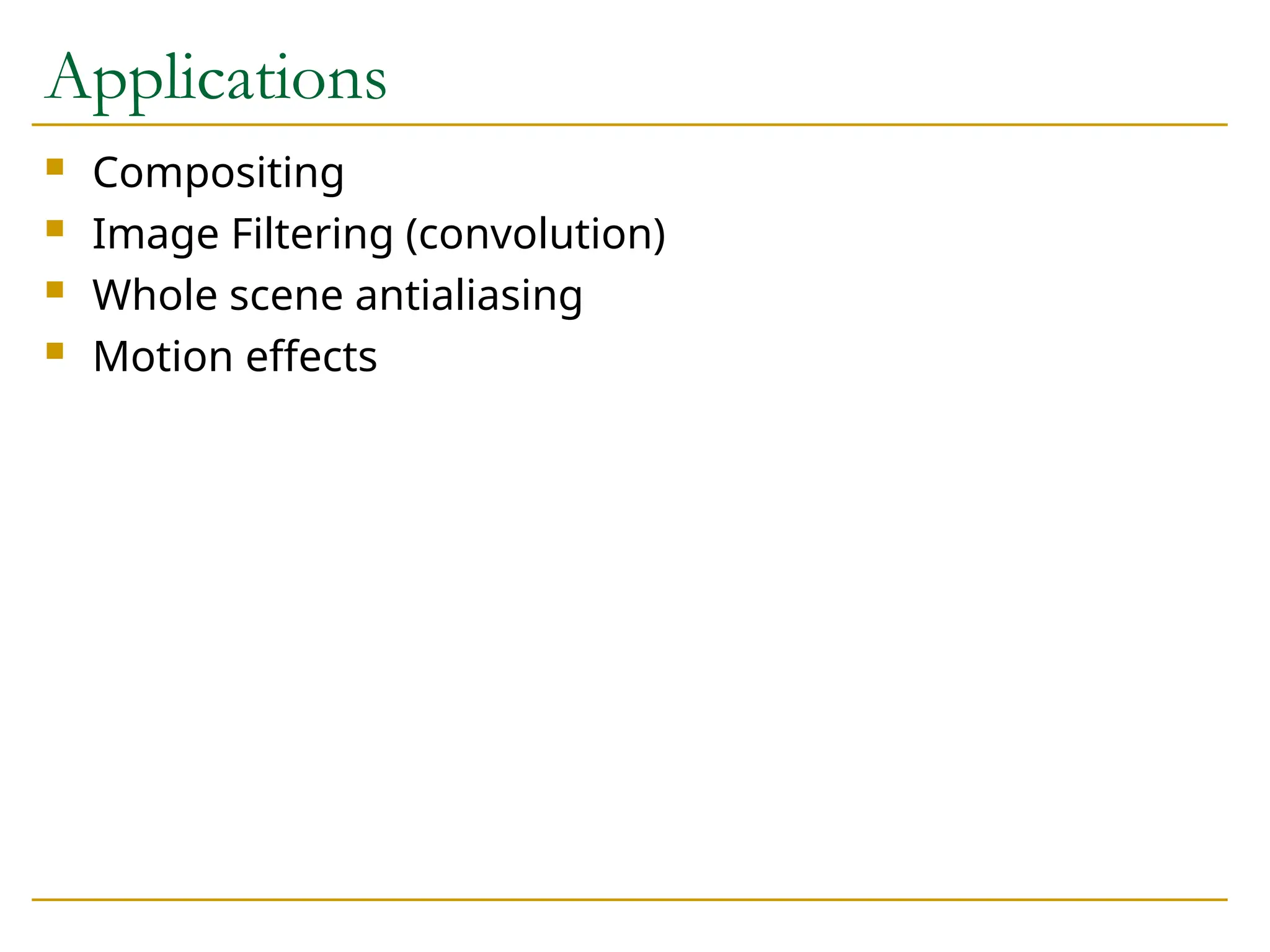
Accumulation Buffer
 Compositing and blending are limited by resolution of the frame
buffer
 Typically 8 bits per color component
 The accumulation buffer is a high resolution buffer (16 or more bits
per component) that avoids this problem
 Write into it or read from it with a scale factor
 Slower than direct compositing into the frame buffer

min
xw max
xw
min
yw
max
yw
Clipping Window
min
xv max
xv
min
yv
max
yv
Viewport
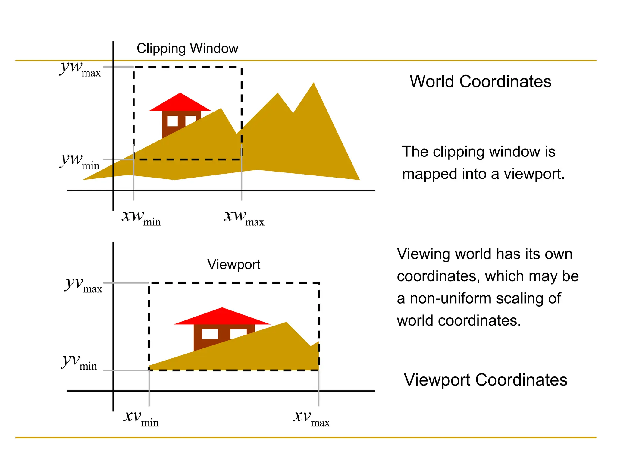
Viewport Coordinates
The clipping window is
mapped into a viewport.
Viewing world has its own
coordinates, which may be
a non-uniform scaling of
world coordinates.
World Coordinates

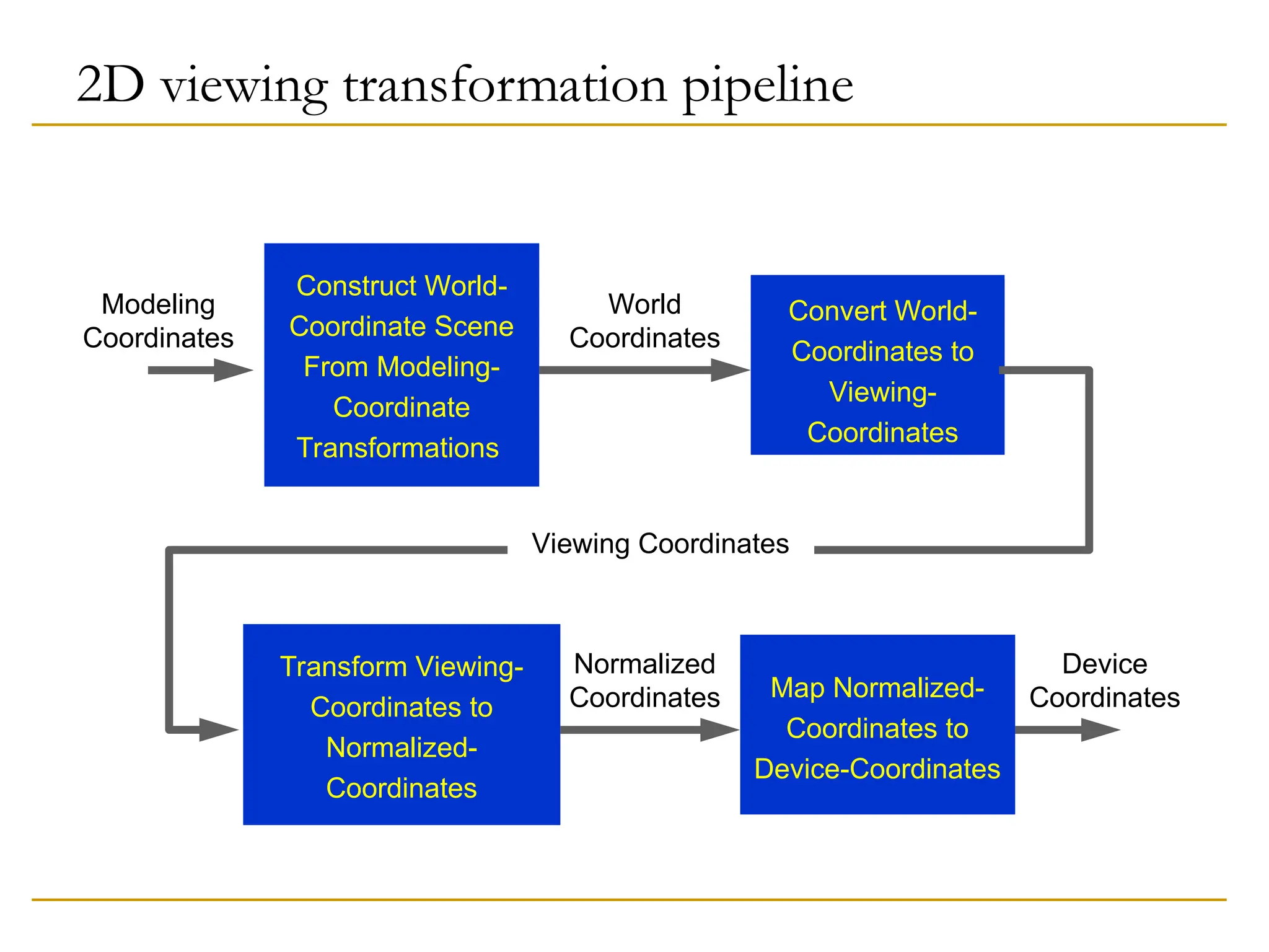
2D viewing transformation pipeline
Construct World-
Coordinate Scene
From Modeling-
Coordinate
Transformations
World
Coordinates
Modeling
Coordinates
Convert World-
Coordinates to
Viewing-
Coordinates
Viewing Coordinates
Transform Viewing-
Coordinates to
Normalized-
Coordinates
Normalized
Coordinates Map Normalized-
Coordinates to
Device-Coordinates
Device
Coordinates

Normalization and Viewport Transformations
 First approach:
 Normalization and window-to-viewport transformations are
combined into one operation.
 Viewport range can be in [0,1] x [0,1].
 Clipping takes place in [0,1] x [0,1].
 Viewport is then mapped to display device.
 Second approach:
 Normalization and clipping take place before viewport
transformation.
 Viewport coordinates are specified in screen coordinates.

Cohen-Sutherland Line Clipping Algorithm
 Intersection calculations are expensive. Find first
lines completely inside or certainly outside clipping
window. Apply intersection only to undecided lines.
 Perform cheaper tests before proceeding to
expensive intersection calculations.

Cohen-Sutherland Line Clipping Algorithm
 Assign code to every endpoint of line segment.
 Borderlines of clipping window divide the plane into two halves.
 A point can be characterized by a 4-bit code according to its
location in half planes.
 Location bit is 0 if the point is in the positive half plane, 1
otherwise.
 Code assignment involves comparisons or subtractions.
 Completely inside / certainly outside tests involve only
logic operations of bits.

Lines that cannot be decided are intersected with window
border lines.
Each test clips the line and the remaining is tested again
for full inclusion or certain exclusion, until remaining is
either empty or fully contained.
Endpoints of lines are examined against left, right, bottom
and top borders (can be any order).

 
0 0
,
x y
 
end end
,
x y
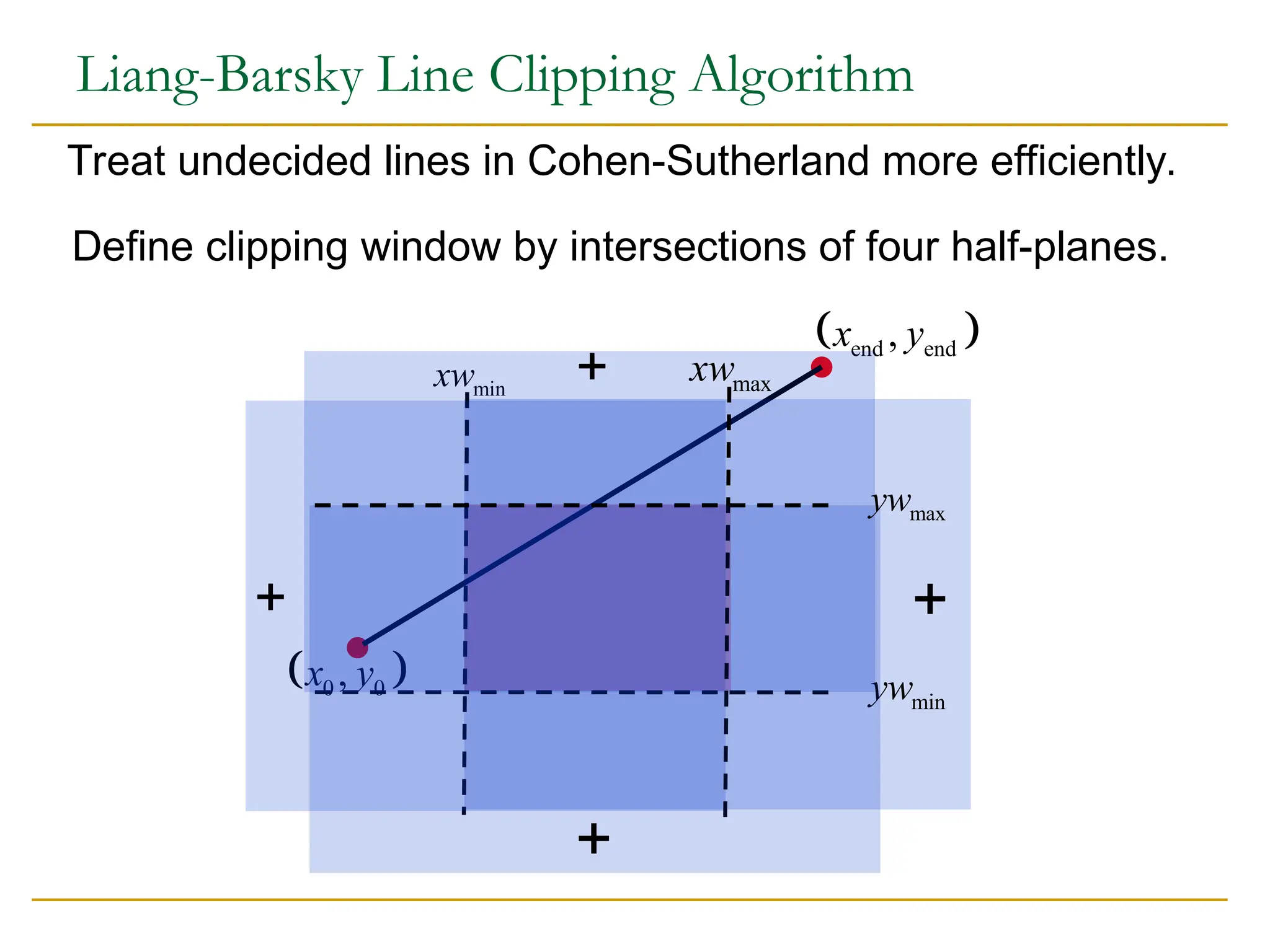
Liang-Barsky Line Clipping Algorithm
Define clipping window by intersections of four half-planes.
Treat undecided lines in Cohen-Sutherland more efficiently.
min
xw

min
yw
 max
xw

max
yw


This is more efficient than Cohen-Sutherland Alg,
which computes intersection with clipping window
borders for each undecided line, as a part of the
feasibility tests.

Nicholl-Lee-Nicholl Line Clipping Algorithm
 Creates more regions around clipping window to
avoid multiple line intersection calculations.
 Performs fewer comparisons and divisions than
Cohen-Sutherland and Liang-Barsky, but cannot be
extended to 3D, while they can.
 For complete inclusion in clipping window or
certain exclusion we’ll use Cohen-Sutherland.

 The four clippers can work in parallel.
 Once a pair of endpoints it output by the first
clipper, the second clipper can start working.
 The more edges in a polygon, the more effective
parallelism is.
 Processing of a new polygon can start once
first clipper finished processing.
 No need to wait for polygon completion.

If and belong to the
same sickle, the intersection point terminating the sickle
must be found since algorithm never ADVANCE along
the polygon whose current edge may contain
i j
p q
Correcness of algorithm :
a sought
intersection point.
This in turn guarantees that once an intersection point
of a sickle is found, all the others will be constructed
successively.

3D Viewing Concepts
World Coordinate System Viewing Coordinate
System

Choose viewing position, direction and orientation of the
camera in the world.
A clipping window is defined by the size of the aperture
and the lens.
Viewing by computing offers many more options which
camera cannot, e.g., parallel or perspective projections,
hiding parts of the scene, viewing behind obstacles, etc.
2D Reminder

Clipping window: Selects what we want to see.
Viewport: Indicates where it is to be viewed on the output
device (still in world coordinates).
Display window: Setting into screen coordinates.
In 3D the clipping is displayed on the view plane, but
clipping of the scene takes place in the space by a clipping
volume.
3D transformation pipeline is similar to 2D with addition of
projection transformation.

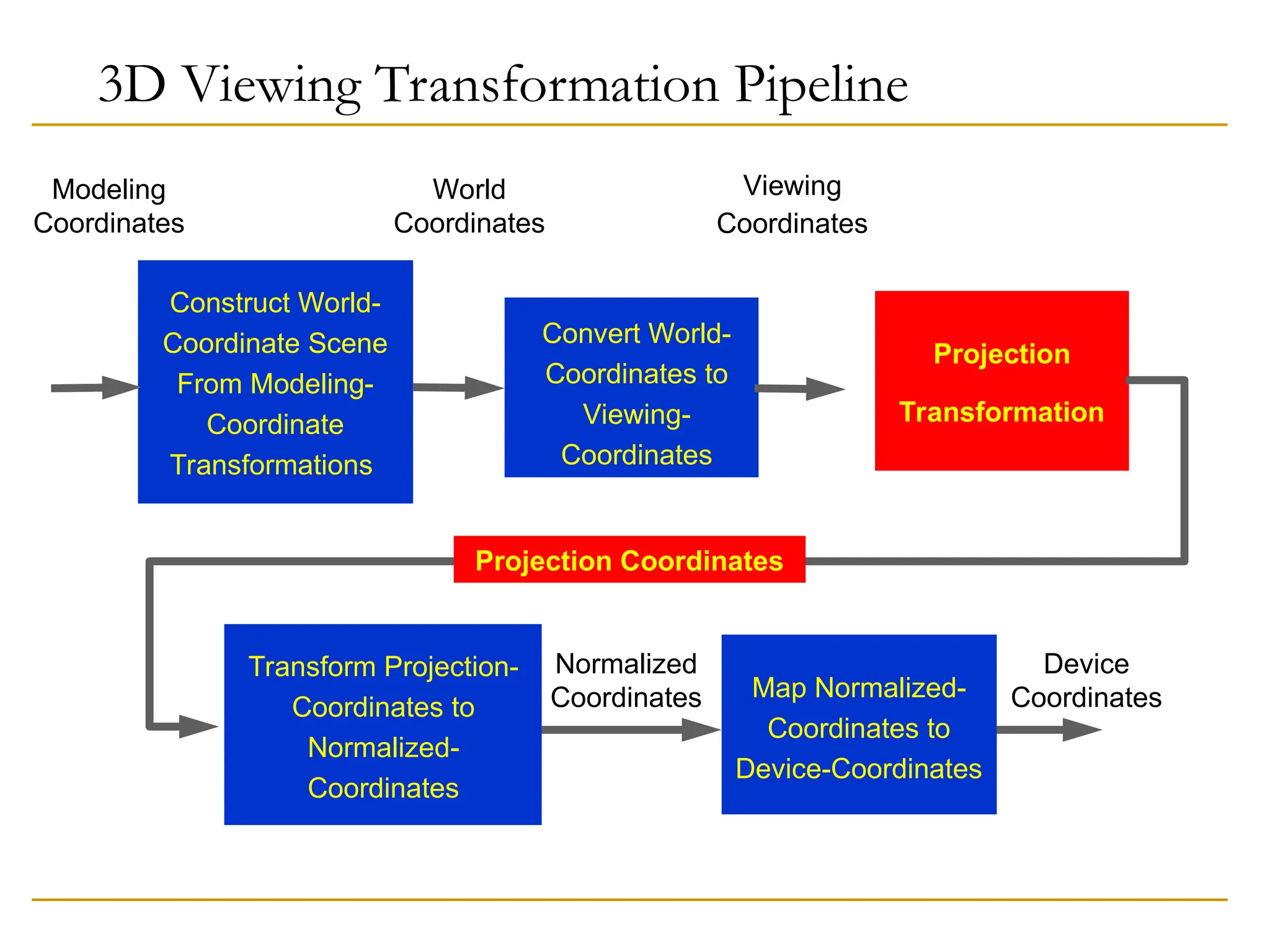
3D Viewing Transformation Pipeline
Transform Projection-
Coordinates to
Normalized-
Coordinates
Normalized
Coordinates Map Normalized-
Coordinates to
Device-Coordinates
Device
Coordinates
Construct World-
Coordinate Scene
From Modeling-
Coordinate
Transformations
World
Coordinates
Modeling
Coordinates
Convert World-
Coordinates to
Viewing-
Coordinates
Viewing
Coordinates
Projection
Transformation
Projection Coordinates

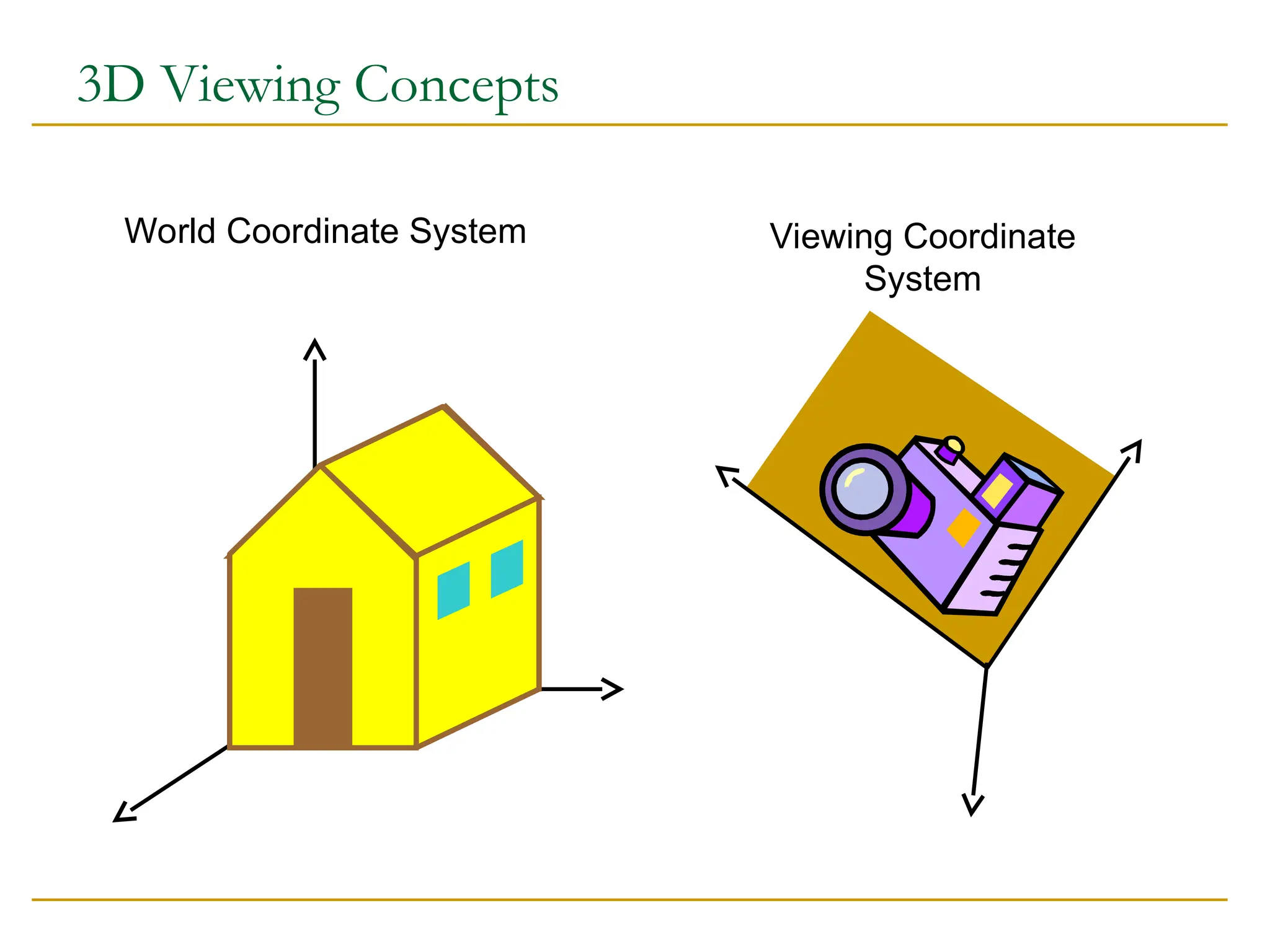
Model is given in model (self) coordinates.
Conversion to world coordinates takes place.
Viewing coordinate system which defines the position and
orientation of the projection plane (film plane in camera) is
selected, to which scene is converted.
2D clipping window (lens of camera) is defined on the
projection plane (film plane) and a 3D clipping, called view
volume, is established.

The shape and size of view volume is defined by the
dimensions of clipping window, the type of projection and
the limiting positions along the viewing direction.
Objects are mapped to normalized coordinated and all
parts of the scene out of the view volume are clipped off.
The clipping is applied after all device independent
transformation are completed, so efficient transformation
concatenation is possible.
Few other tasks such as hidden surface removal and
surface rendering take place along the pipeline.

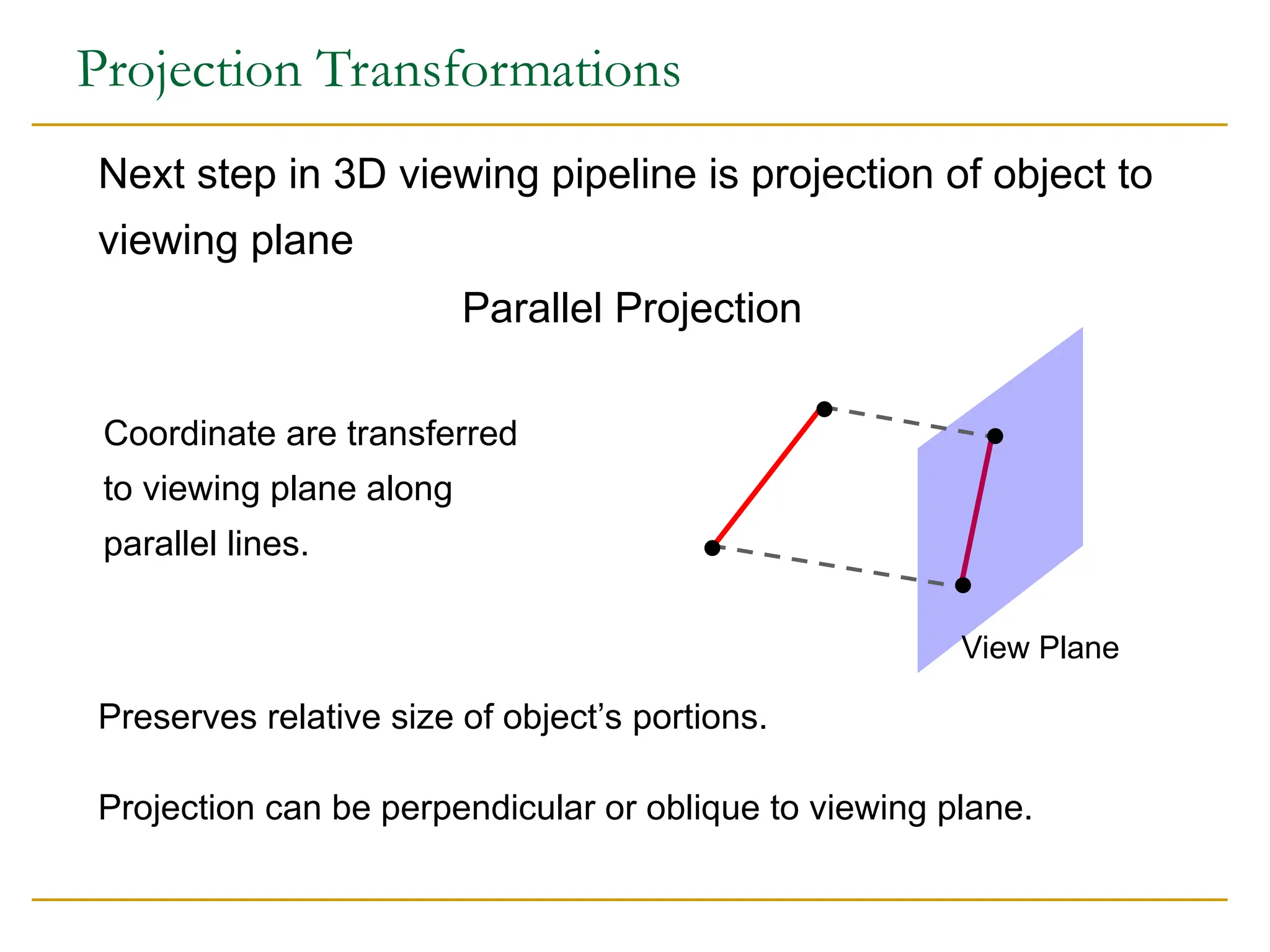
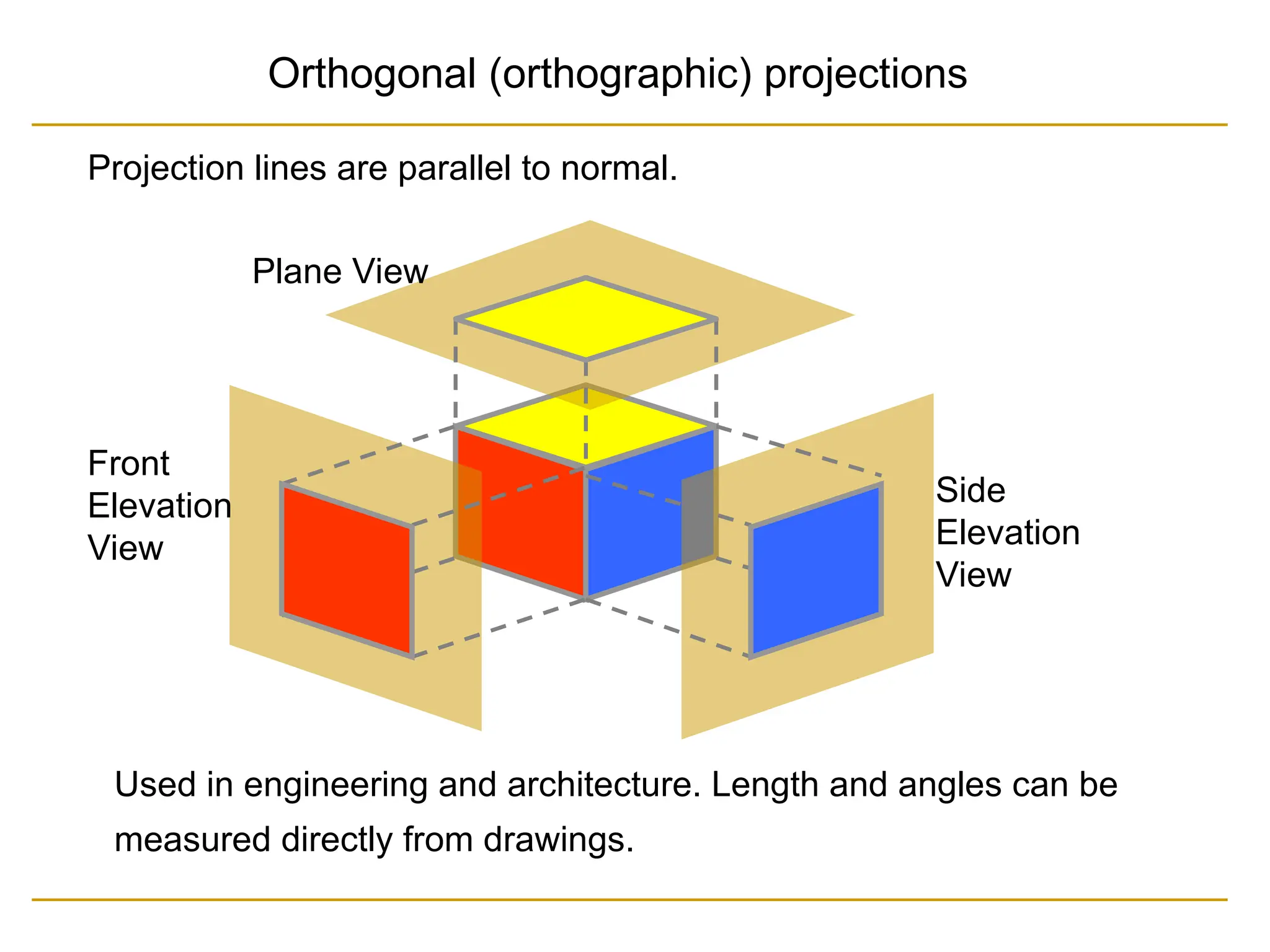
Projection Transformations
Projection can be perpendicular or oblique to viewing plane.
Preserves relative size of object’s portions.
Next step in 3D viewing pipeline is projection of object to
viewing plane
Parallel Projection
Coordinate are transferred
to viewing plane along
parallel lines.
View Plane

Perspective Projection
Projection lines converge
in a point behind viewing
plane.
Doesn’t preserve relative size but looks more realistic.

Plane View
Side
Elevation
View
Front
Elevation
View
Used in engineering and architecture. Length and angles can be
measured directly from drawings.
Orthogonal (orthographic) projections
Projection lines are parallel to normal.

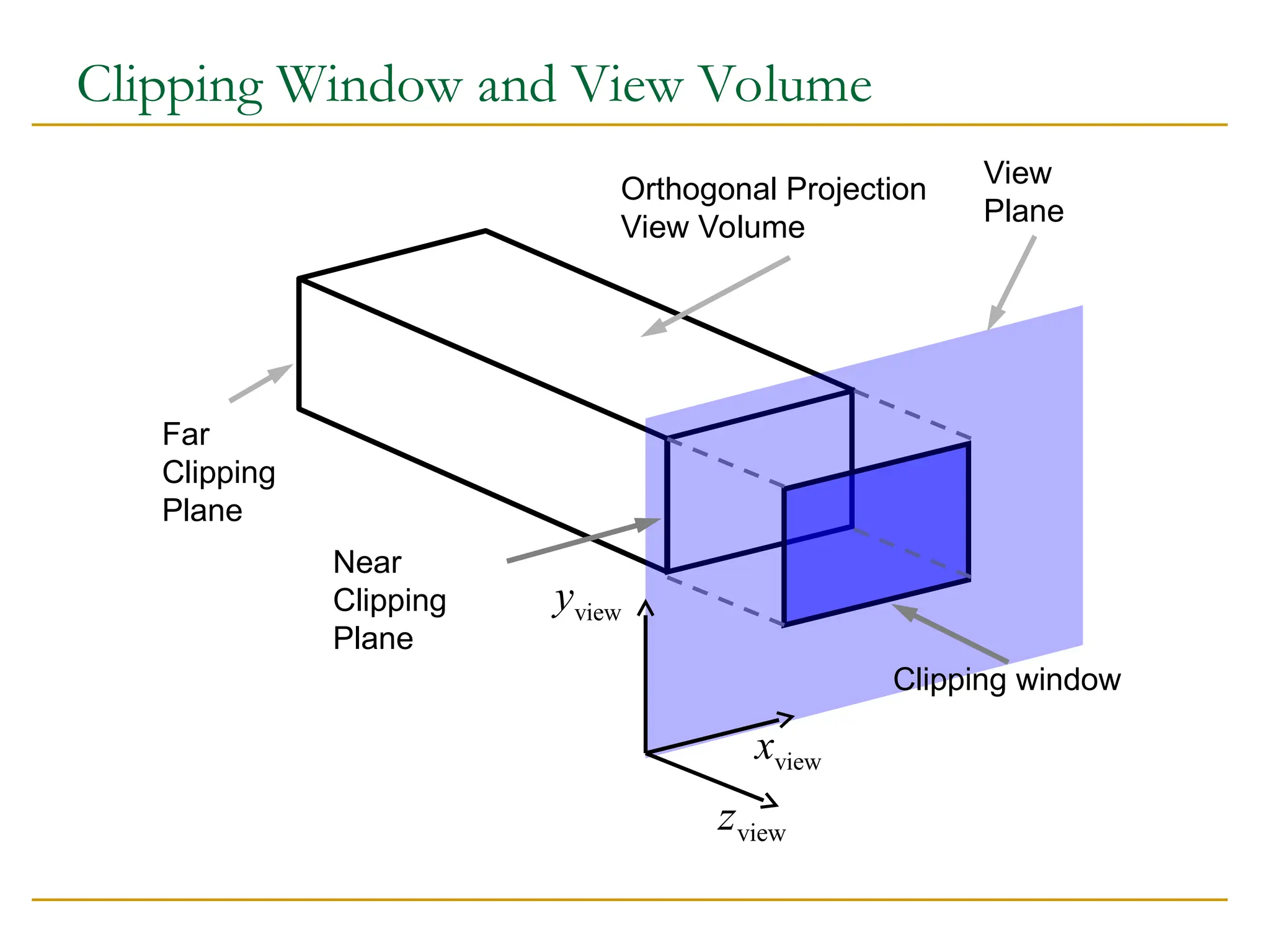
Clipping Window and View Volume
Orthogonal Projection
View Volume
Far
Clipping
Plane
Near
Clipping
Plane
View
Plane
Clipping window
view
x
view
y
view
z

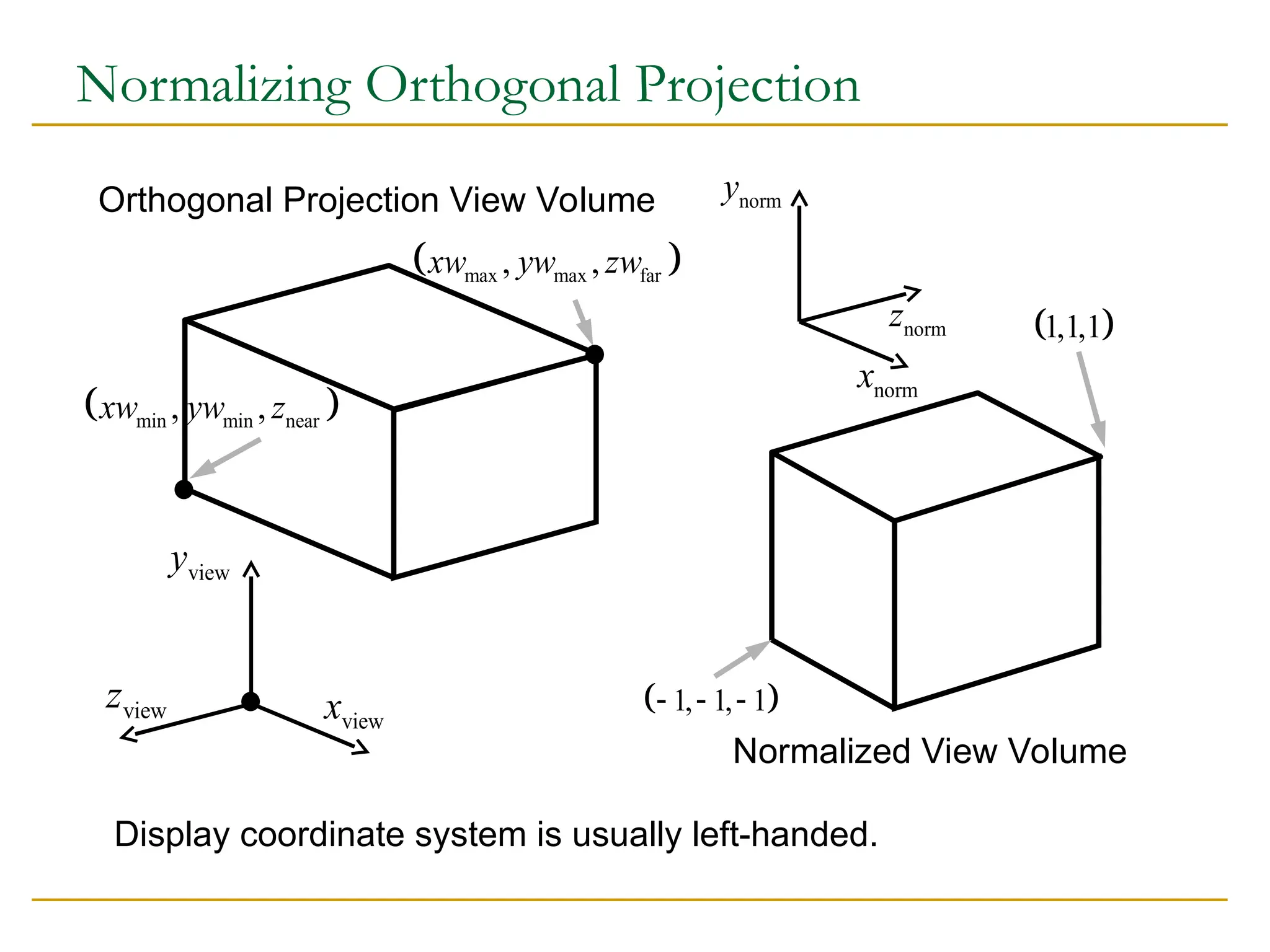
Normalizing Orthogonal Projection
 
1, 1, 1
  
 
1,1,1
norm
z
norm
y
norm
x
Normalized View Volume
Display coordinate system is usually left-handed.
Orthogonal Projection View Volume
view
x
view
y
view
z
 
min min near
, ,
xw yw z
 
max max far
, ,
xw yw zw

The problem with the above representation is that Z appears in
denominator, so matrix multiplication representation of X and Y
on view plane as a function of Z is not straight forward.
Z is point specific, hence division will be computation killer.
Different representation is in order, so transformations can
be concatenated

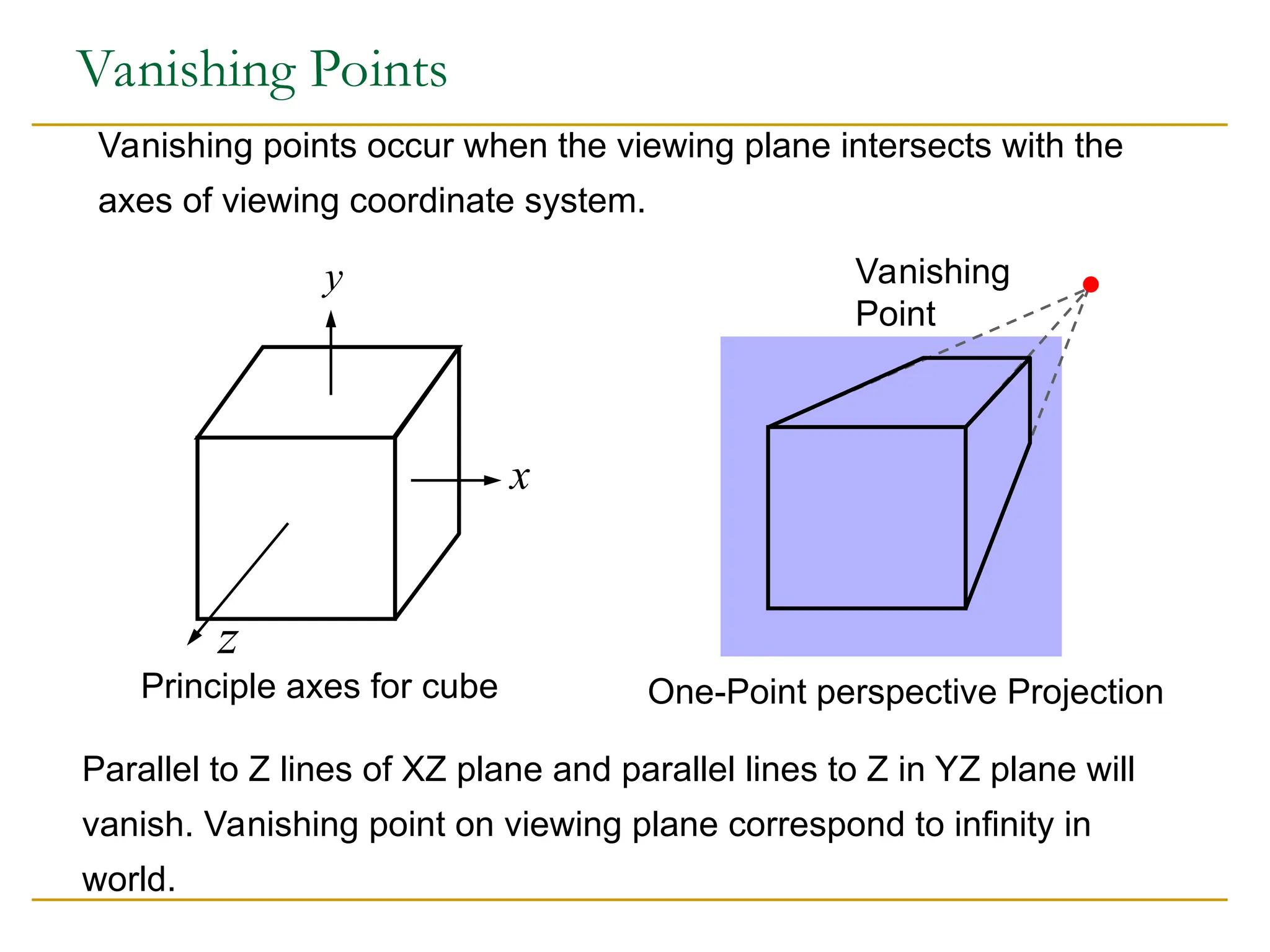
Vanishing Points
Vanishing points occur when the viewing plane intersects with the
axes of viewing coordinate system.
Vanishing
Point
One-Point perspective Projection
x
y
z
Principle axes for cube
Parallel to Z lines of XZ plane and parallel lines to Z in YZ plane will
vanish. Vanishing point on viewing plane correspond to infinity in
world.

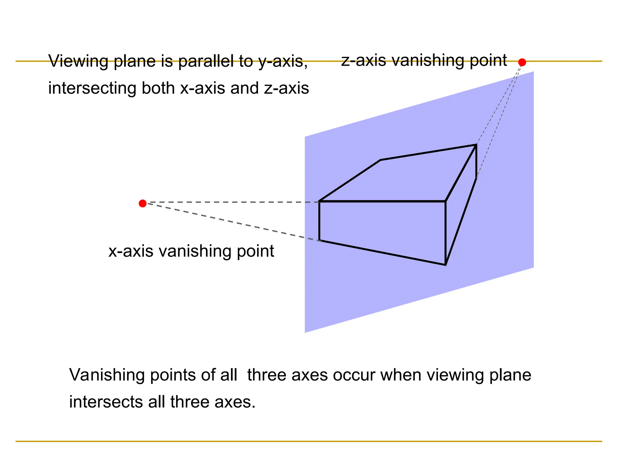
Vanishing points of all three axes occur when viewing plane
intersects all three axes.
x-axis vanishing point
z-axis vanishing point
Viewing plane is parallel to y-axis,
intersecting both x-axis and z-axis

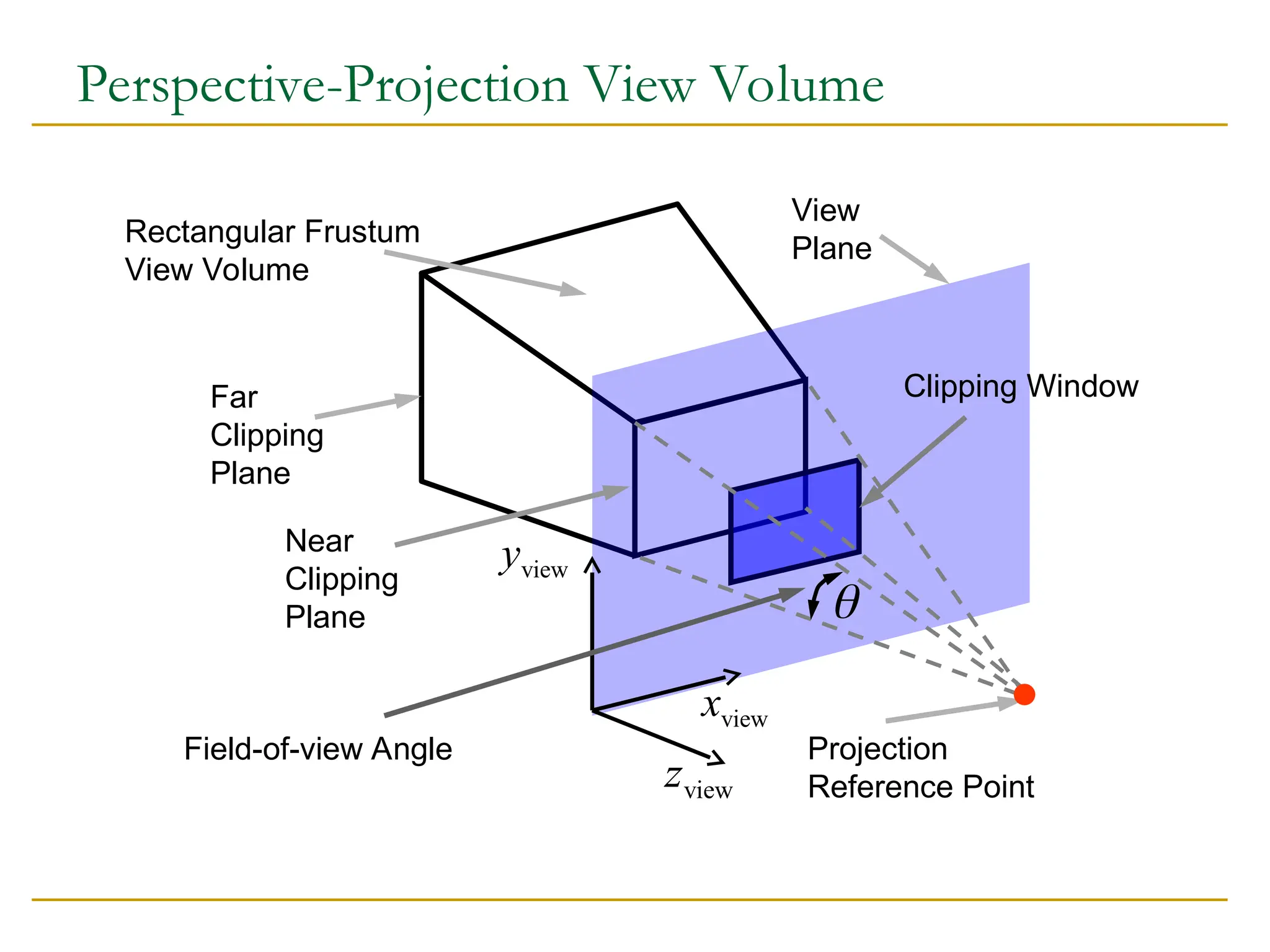
Perspective-Projection View Volume
Rectangular Frustum
View Volume
Far
Clipping
Plane
Near
Clipping
Plane
View
Plane
Clipping Window
view
x
view
y
view
z
Projection
Reference Point

Field-of-view Angle

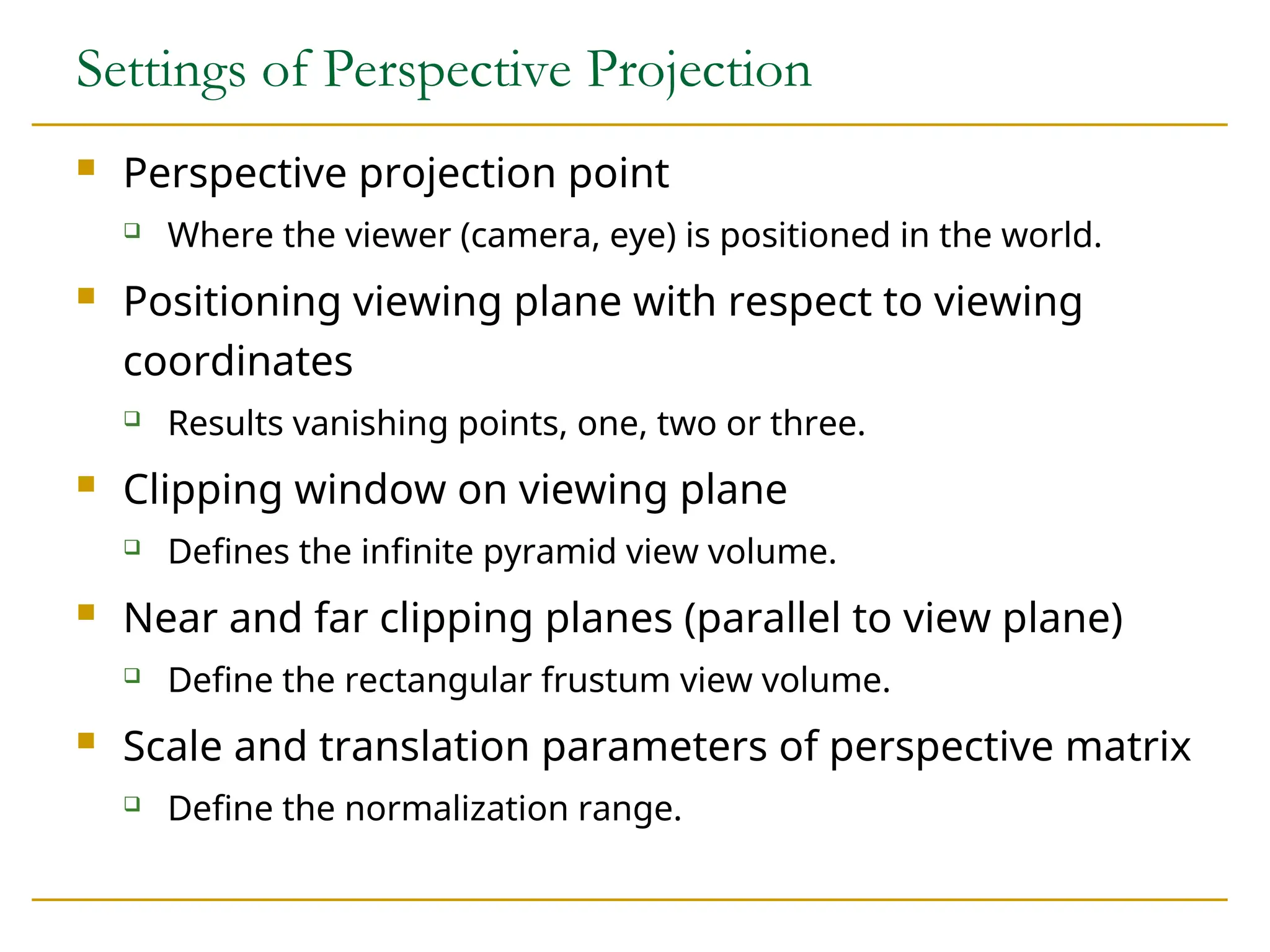
Settings of Perspective Projection
 Perspective projection point
 Where the viewer (camera, eye) is positioned in the world.
 Positioning viewing plane with respect to viewing
coordinates
 Results vanishing points, one, two or three.
 Clipping window on viewing plane
 Defines the infinite pyramid view volume.
 Near and far clipping planes (parallel to view plane)
 Define the rectangular frustum view volume.
 Scale and translation parameters of perspective matrix
 Define the normalization range.

Applications
 Compositing
 Image Filtering (convolution)
 Whole scene antialiasing
 Motion effects

Topic 6 Graphic Transformation and Viewing.ppt

More Related Content

Similar to Topic 6 Graphic Transformation and Viewing.ppt

Recently uploaded

Topic 6 Graphic Transformation and Viewing.ppt