Time series Analysis - State space models and Kalman filtering
1.
Warm-up: Recursive LeastSquares
Kalman Filter
Nonlinear State Space Models
Particle Filtering
Time Series Analysis
5. State space models and Kalman filtering
Andrew Lesniewski
Baruch College
New York
Fall 2019
A. Lesniewski Time Series Analysis
2.
Warm-up: Recursive LeastSquares
Kalman Filter
Nonlinear State Space Models
Particle Filtering
Outline
1 Warm-up: Recursive Least Squares
2 Kalman Filter
3 Nonlinear State Space Models
4 Particle Filtering
A. Lesniewski Time Series Analysis
3.
Warm-up: Recursive LeastSquares
Kalman Filter
Nonlinear State Space Models
Particle Filtering
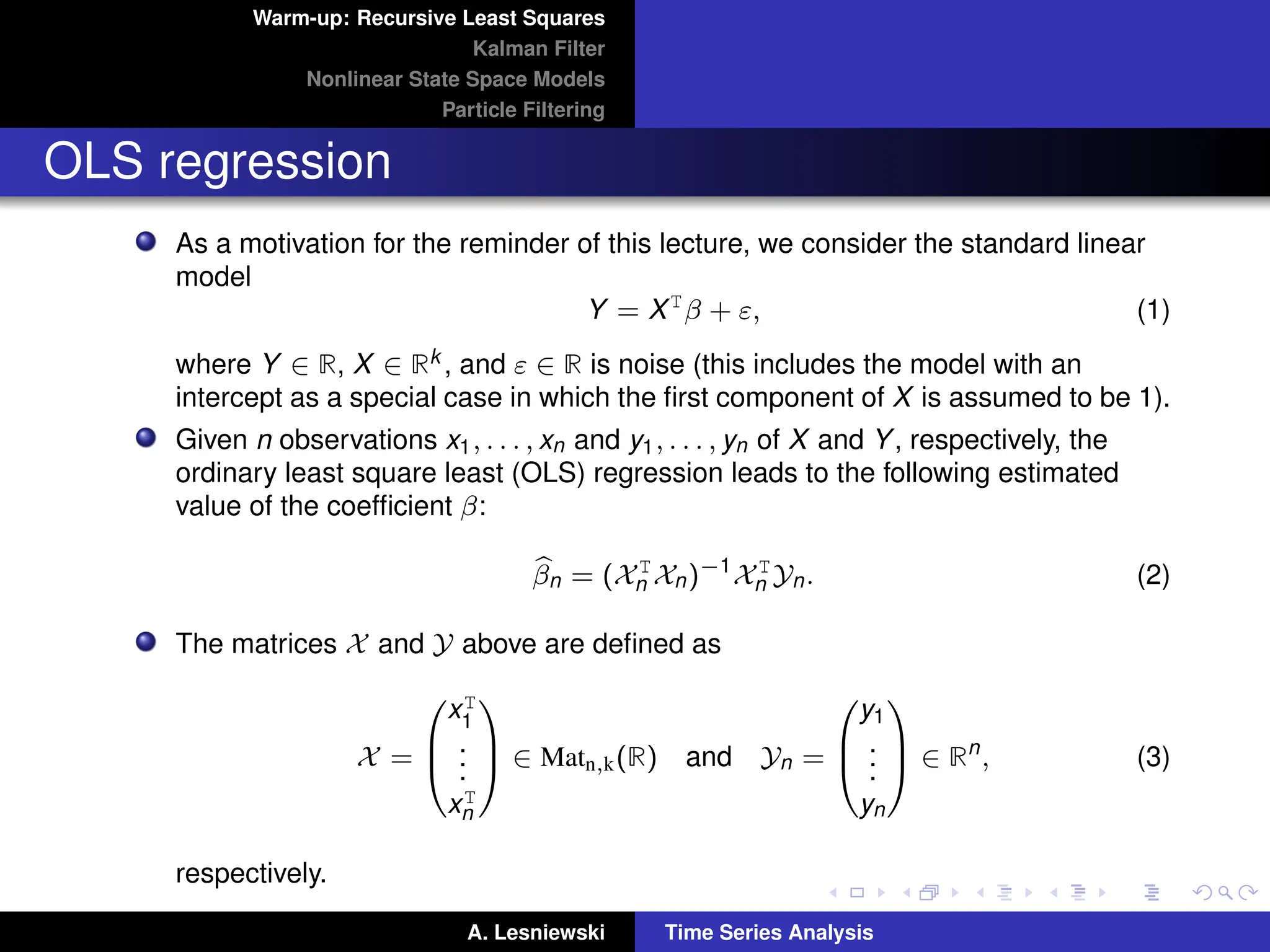
OLS regression
As a motivation for the reminder of this lecture, we consider the standard linear
model
Y = XT
β + ε, (1)
where Y ∈ R, X ∈ Rk , and ε ∈ R is noise (this includes the model with an
intercept as a special case in which the first component of X is assumed to be 1).
Given n observations x1, . . . , xn and y1, . . . , yn of X and Y, respectively, the
ordinary least square least (OLS) regression leads to the following estimated
value of the coefficient β:
b
βn = (XT
n Xn)−1
XT
n Yn. (2)
The matrices X and Y above are defined as
X =
xT
1
.
.
.
xT
n
∈ Matn,k(R) and Yn =
y1
.
.
.
yn
∈ Rn
, (3)
respectively.
A. Lesniewski Time Series Analysis
4.
Warm-up: Recursive LeastSquares
Kalman Filter
Nonlinear State Space Models
Particle Filtering
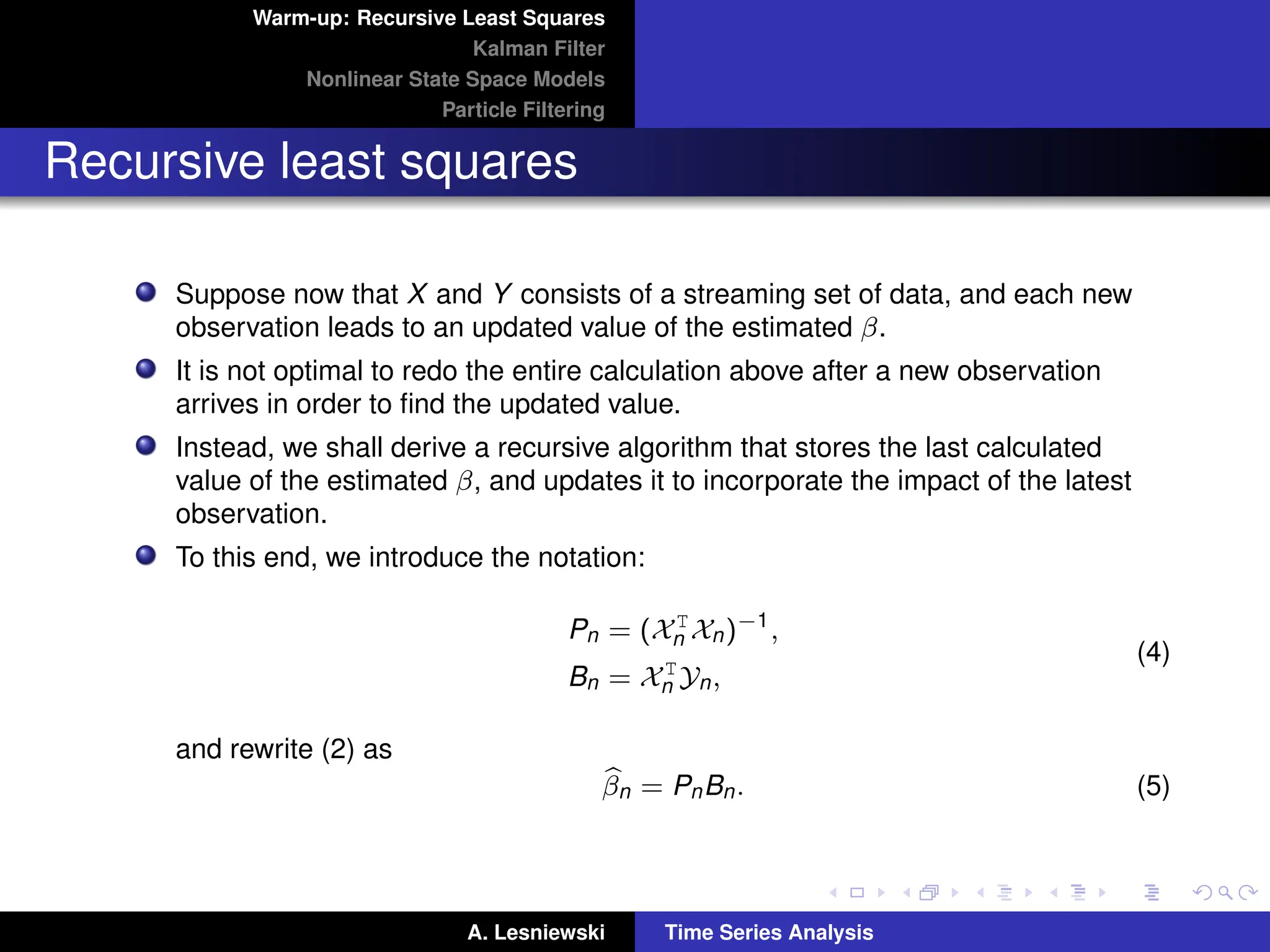
Recursive least squares
Suppose now that X and Y consists of a streaming set of data, and each new
observation leads to an updated value of the estimated β.
It is not optimal to redo the entire calculation above after a new observation
arrives in order to find the updated value.
Instead, we shall derive a recursive algorithm that stores the last calculated
value of the estimated β, and updates it to incorporate the impact of the latest
observation.
To this end, we introduce the notation:
Pn = (XT
n Xn)−1
,
Bn = XT
n Yn,
(4)
and rewrite (2) as
b
βn = PnBn. (5)
A. Lesniewski Time Series Analysis
5.
Warm-up: Recursive LeastSquares
Kalman Filter
Nonlinear State Space Models
Particle Filtering
Recursive least squares
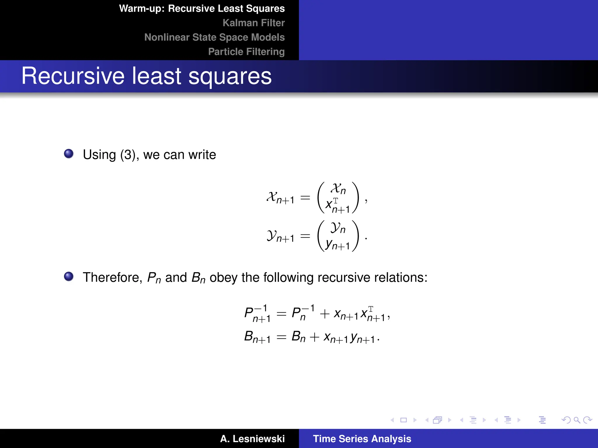
Using (3), we can write
Xn+1 =
Xn
xT
n+1
,
Yn+1 =
Yn
yn+1
.
Therefore, Pn and Bn obey the following recursive relations:
P−1
n+1 = P−1
n + xn+1xT
n+1,
Bn+1 = Bn + xn+1yn+1.
A. Lesniewski Time Series Analysis
6.
Warm-up: Recursive LeastSquares
Kalman Filter
Nonlinear State Space Models
Particle Filtering
Recursive least squares
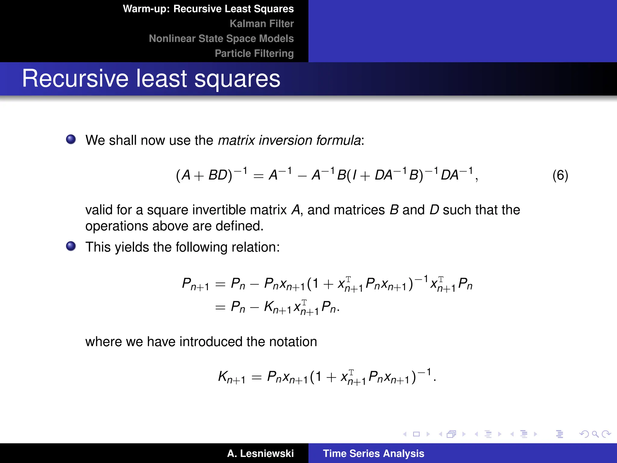
We shall now use the matrix inversion formula:
(A + BD)−1
= A−1
− A−1
B(I + DA−1
B)−1
DA−1
, (6)
valid for a square invertible matrix A, and matrices B and D such that the
operations above are defined.
This yields the following relation:
Pn+1 = Pn − Pnxn+1(1 + xT
n+1Pnxn+1)−1
xT
n+1Pn
= Pn − Kn+1xT
n+1Pn.
where we have introduced the notation
Kn+1 = Pnxn+1(1 + xT
n+1Pnxn+1)−1
.
A. Lesniewski Time Series Analysis
7.
Warm-up: Recursive LeastSquares
Kalman Filter
Nonlinear State Space Models
Particle Filtering
Recursive least squares
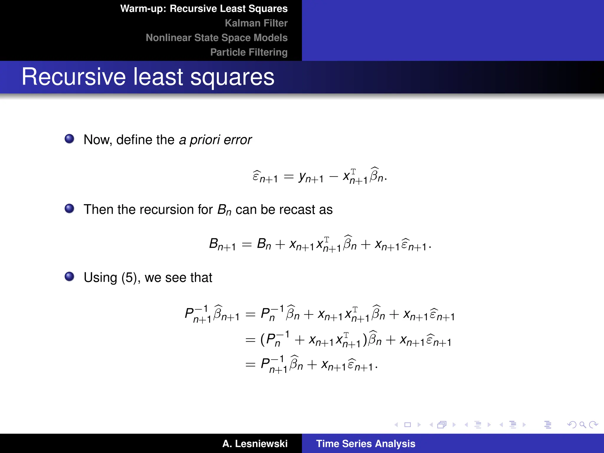
Now, define the a priori error
b
εn+1 = yn+1 − xT
n+1
b
βn.
Then the recursion for Bn can be recast as
Bn+1 = Bn + xn+1xT
n+1
b
βn + xn+1b
εn+1.
Using (5), we see that
P−1
n+1
b
βn+1 = P−1
n
b
βn + xn+1xT
n+1
b
βn + xn+1b
εn+1
= (P−1
n + xn+1xT
n+1)b
βn + xn+1b
εn+1
= P−1
n+1
b
βn + xn+1b
εn+1.
A. Lesniewski Time Series Analysis
8.
Warm-up: Recursive LeastSquares
Kalman Filter
Nonlinear State Space Models
Particle Filtering
Recursive least squares
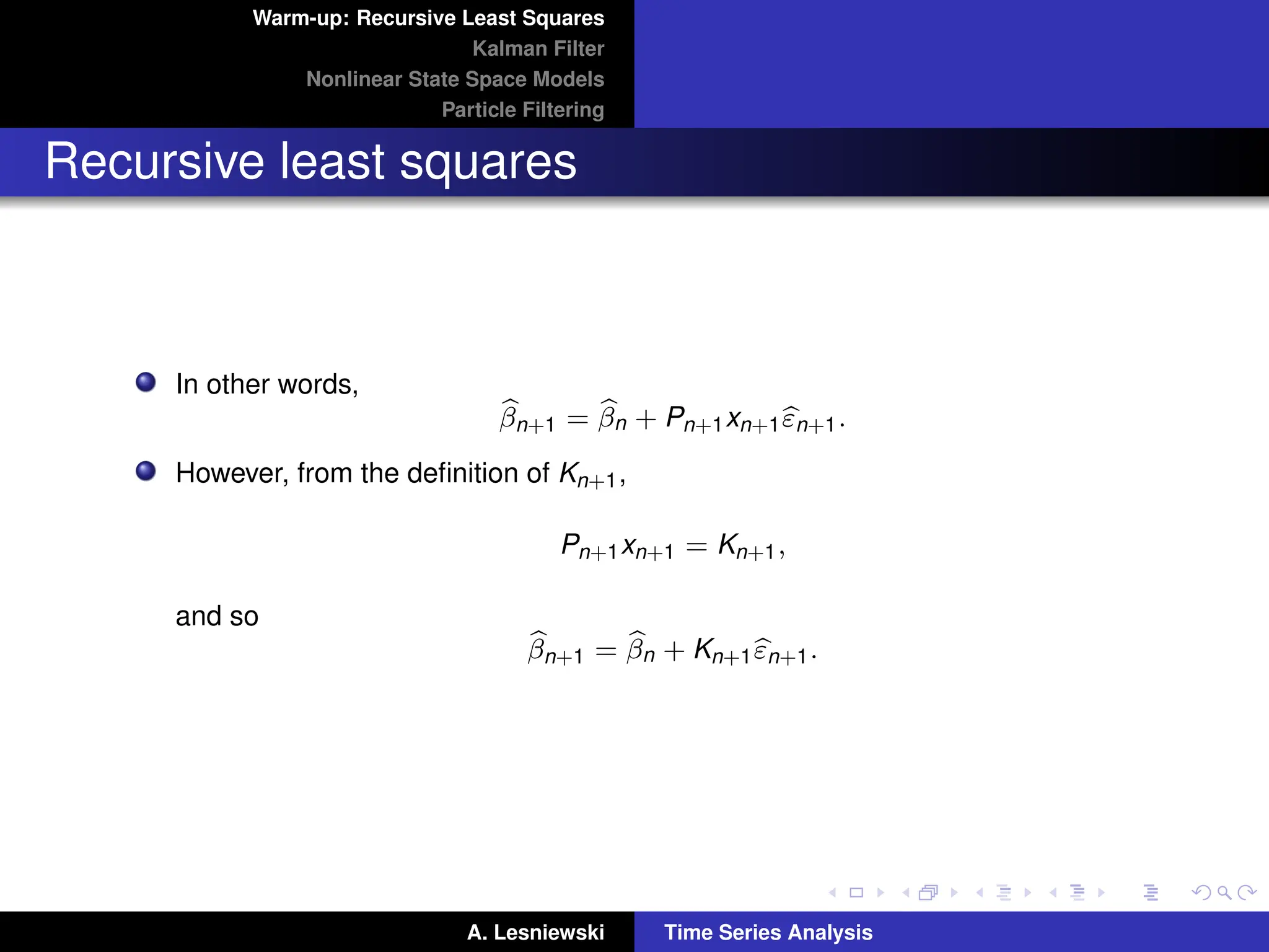
In other words,
b
βn+1 = b
βn + Pn+1xn+1b
εn+1.
However, from the definition of Kn+1,
Pn+1xn+1 = Kn+1,
and so
b
βn+1 = b
βn + Kn+1b
εn+1.
A. Lesniewski Time Series Analysis
9.
Warm-up: Recursive LeastSquares
Kalman Filter
Nonlinear State Space Models
Particle Filtering
Recursive least squares
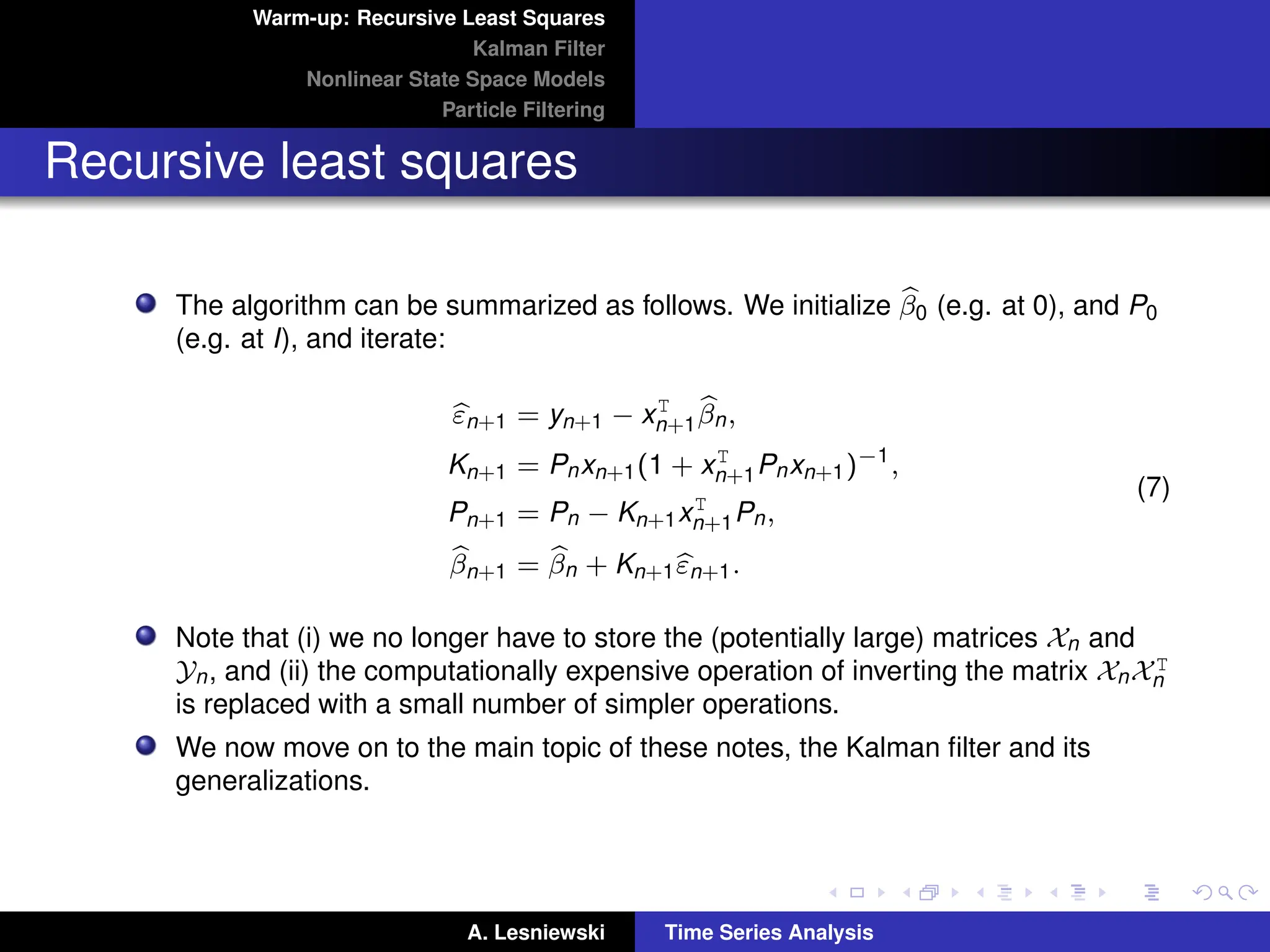
The algorithm can be summarized as follows. We initialize b
β0 (e.g. at 0), and P0
(e.g. at I), and iterate:
b
εn+1 = yn+1 − xT
n+1
b
βn,
Kn+1 = Pnxn+1(1 + xT
n+1Pnxn+1)−1
,
Pn+1 = Pn − Kn+1xT
n+1Pn,
b
βn+1 = b
βn + Kn+1b
εn+1.
(7)
Note that (i) we no longer have to store the (potentially large) matrices Xn and
Yn, and (ii) the computationally expensive operation of inverting the matrix XnXT
n
is replaced with a small number of simpler operations.
We now move on to the main topic of these notes, the Kalman filter and its
generalizations.
A. Lesniewski Time Series Analysis
10.
Warm-up: Recursive LeastSquares
Kalman Filter
Nonlinear State Space Models
Particle Filtering
State space models
A state space model (SSM) is a time series model in which the time series Yt is
interpreted as the result of a noisy observation of a stochastic process Xt .
The values of the variables Xt and Yt can be continuous (scalar or vector) or
discrete.
Graphically, an SSM is represented as follows:
X1 → X2 → . . . → Xt → . . . state process
y
y
y
y · · ·
Y1 Y2 . . . Yt . . . observation process
(8)
SSMs belong to the realm of Bayesian inference, and they have been
successfully applied in many fields to solve a broad range of problems.
Our discussion of SSMs follows largely [2].
A. Lesniewski Time Series Analysis
11.
Warm-up: Recursive LeastSquares
Kalman Filter
Nonlinear State Space Models
Particle Filtering
State space models
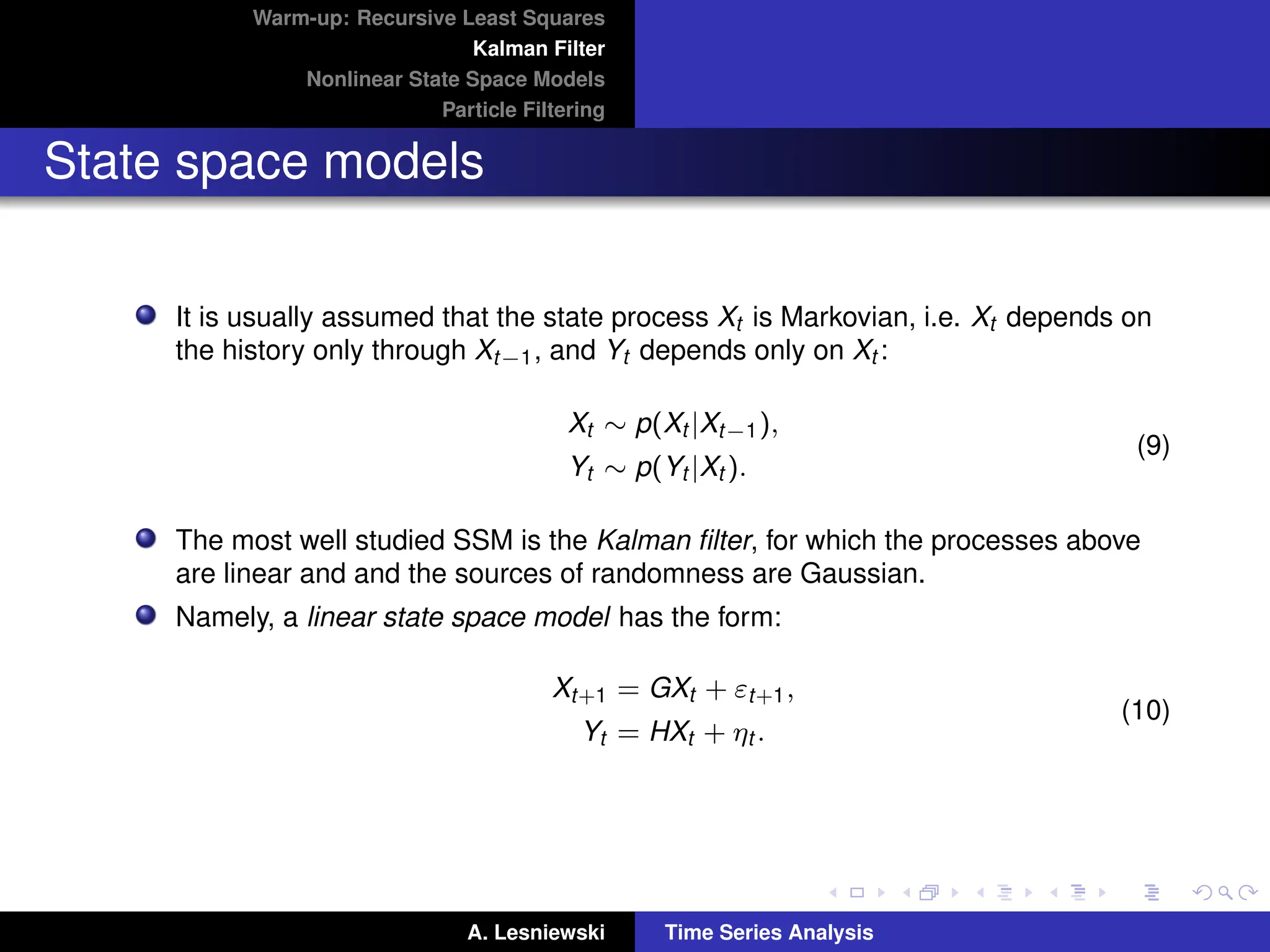
It is usually assumed that the state process Xt is Markovian, i.e. Xt depends on
the history only through Xt−1, and Yt depends only on Xt :
Xt ∼ p(Xt |Xt−1),
Yt ∼ p(Yt |Xt ).
(9)
The most well studied SSM is the Kalman filter, for which the processes above
are linear and and the sources of randomness are Gaussian.
Namely, a linear state space model has the form:
Xt+1 = GXt + εt+1,
Yt = HXt + ηt .
(10)
A. Lesniewski Time Series Analysis
12.
Warm-up: Recursive LeastSquares
Kalman Filter
Nonlinear State Space Models
Particle Filtering
State space models
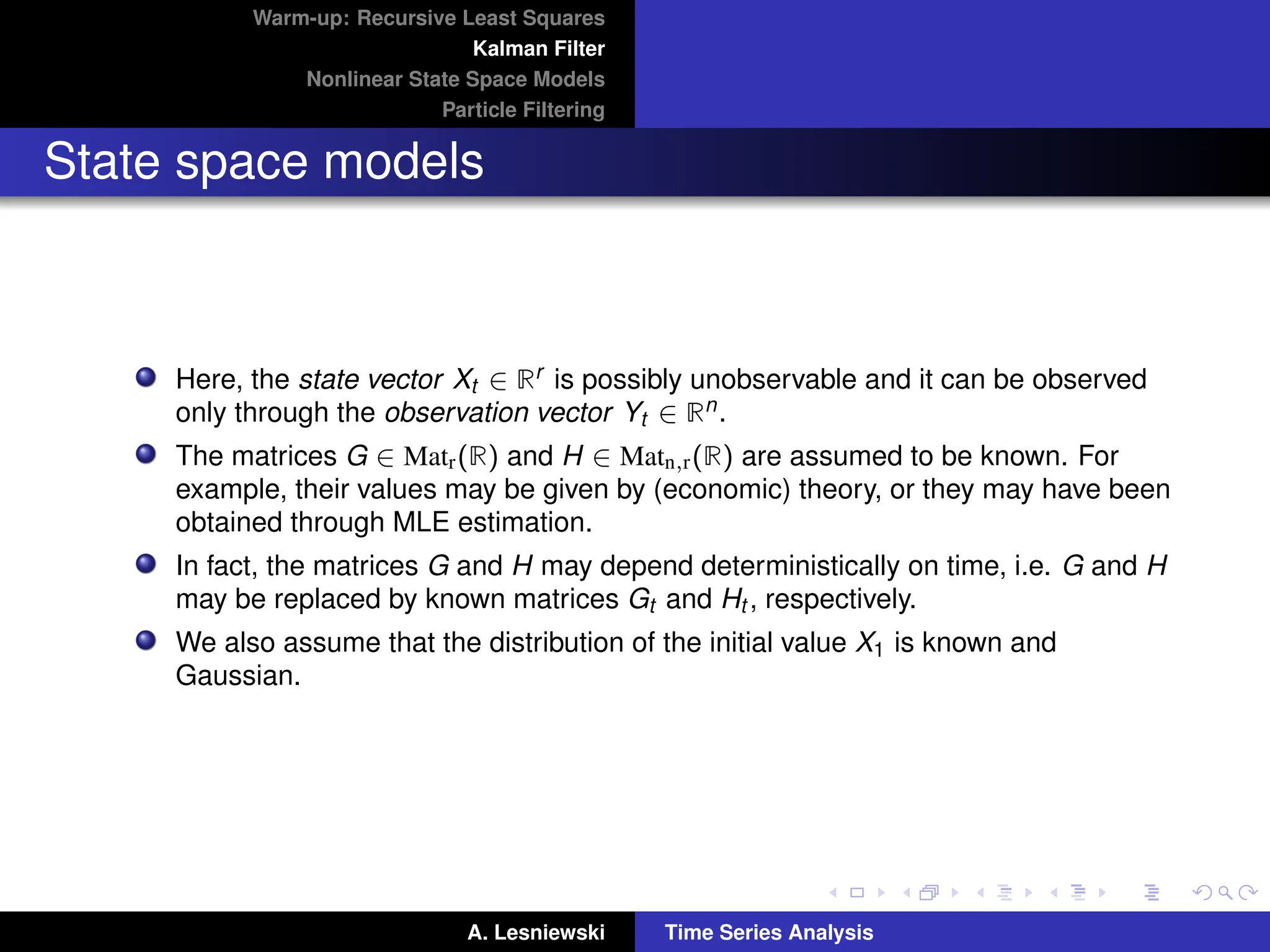
Here, the state vector Xt ∈ Rr is possibly unobservable and it can be observed
only through the observation vector Yt ∈ Rn.
The matrices G ∈ Matr(R) and H ∈ Matn,r(R) are assumed to be known. For
example, their values may be given by (economic) theory, or they may have been
obtained through MLE estimation.
In fact, the matrices G and H may depend deterministically on time, i.e. G and H
may be replaced by known matrices Gt and Ht , respectively.
We also assume that the distribution of the initial value X1 is known and
Gaussian.
A. Lesniewski Time Series Analysis
13.
Warm-up: Recursive LeastSquares
Kalman Filter
Nonlinear State Space Models
Particle Filtering
State space models
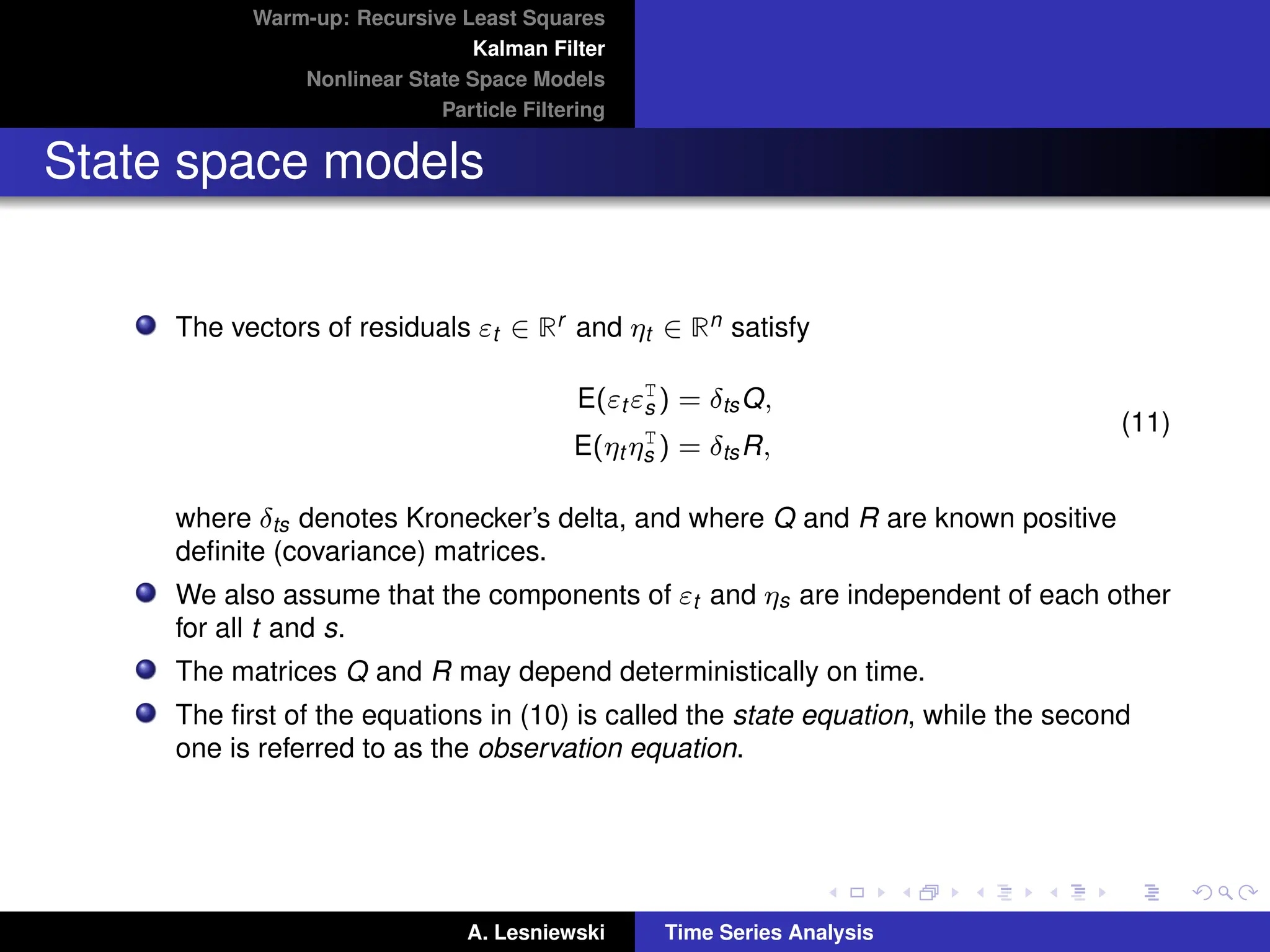
The vectors of residuals εt ∈ Rr and ηt ∈ Rn satisfy
E(εt εT
s ) = δtsQ,
E(ηt ηT
s ) = δtsR,
(11)
where δts denotes Kronecker’s delta, and where Q and R are known positive
definite (covariance) matrices.
We also assume that the components of εt and ηs are independent of each other
for all t and s.
The matrices Q and R may depend deterministically on time.
The first of the equations in (10) is called the state equation, while the second
one is referred to as the observation equation.
A. Lesniewski Time Series Analysis
14.
Warm-up: Recursive LeastSquares
Kalman Filter
Nonlinear State Space Models
Particle Filtering
Inference for state space models
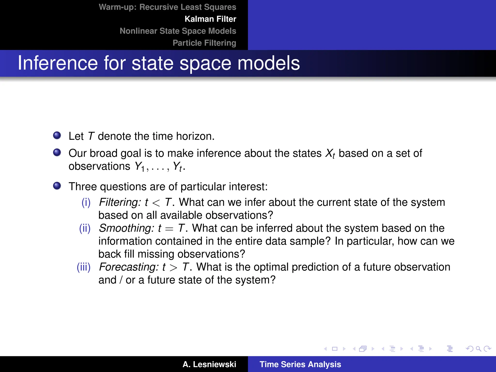
Let T denote the time horizon.
Our broad goal is to make inference about the states Xt based on a set of
observations Y1, . . . , Yt .
Three questions are of particular interest:
(i) Filtering: t T. What can we infer about the current state of the system
based on all available observations?
(ii) Smoothing: t = T. What can be inferred about the system based on the
information contained in the entire data sample? In particular, how can we
back fill missing observations?
(iii) Forecasting: t T. What is the optimal prediction of a future observation
and / or a future state of the system?
A. Lesniewski Time Series Analysis
15.
Warm-up: Recursive LeastSquares
Kalman Filter
Nonlinear State Space Models
Particle Filtering
Kalman filter
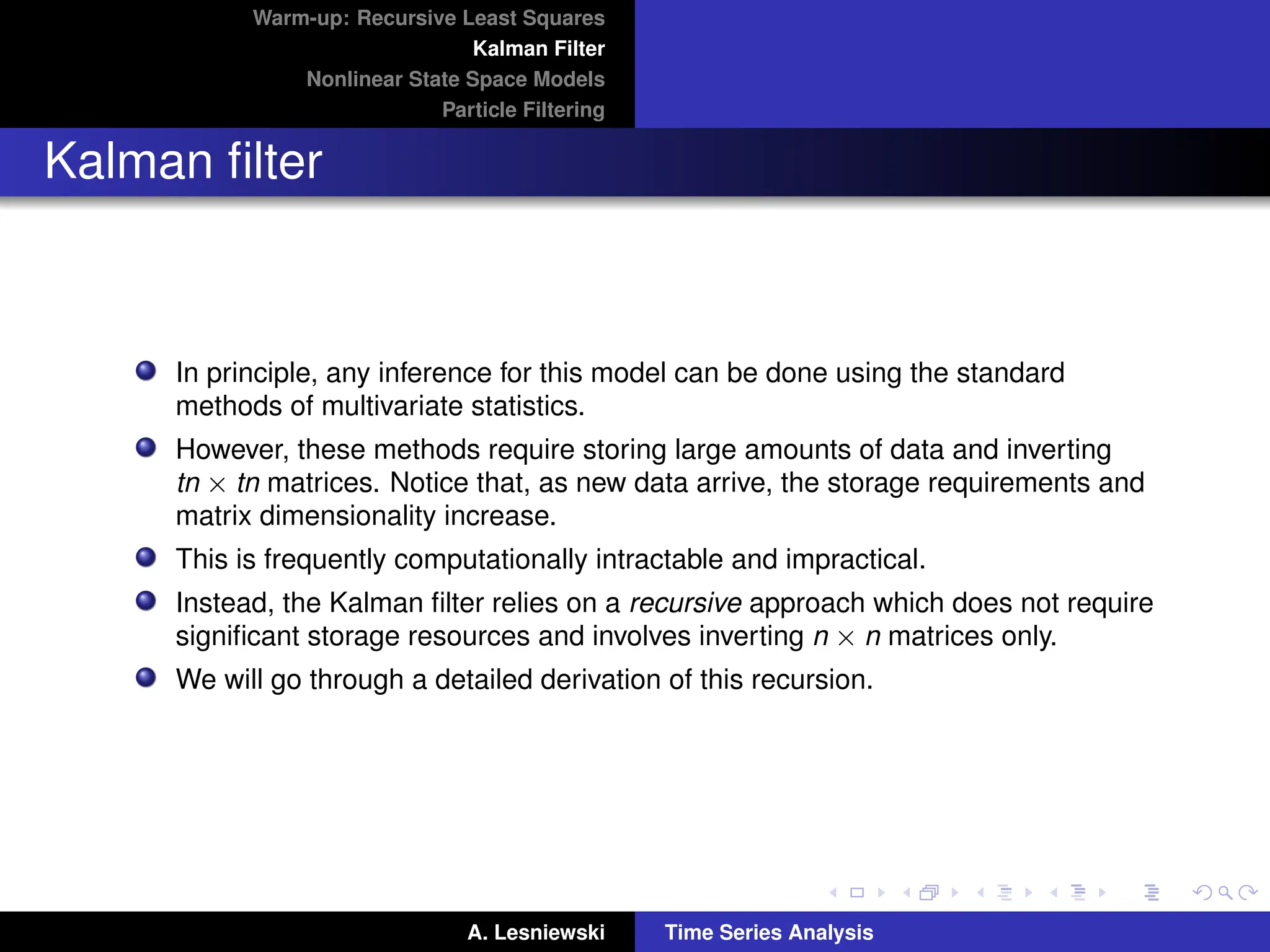
In principle, any inference for this model can be done using the standard
methods of multivariate statistics.
However, these methods require storing large amounts of data and inverting
tn × tn matrices. Notice that, as new data arrive, the storage requirements and
matrix dimensionality increase.
This is frequently computationally intractable and impractical.
Instead, the Kalman filter relies on a recursive approach which does not require
significant storage resources and involves inverting n × n matrices only.
We will go through a detailed derivation of this recursion.
A. Lesniewski Time Series Analysis
16.
Warm-up: Recursive LeastSquares
Kalman Filter
Nonlinear State Space Models
Particle Filtering
Kalman filter
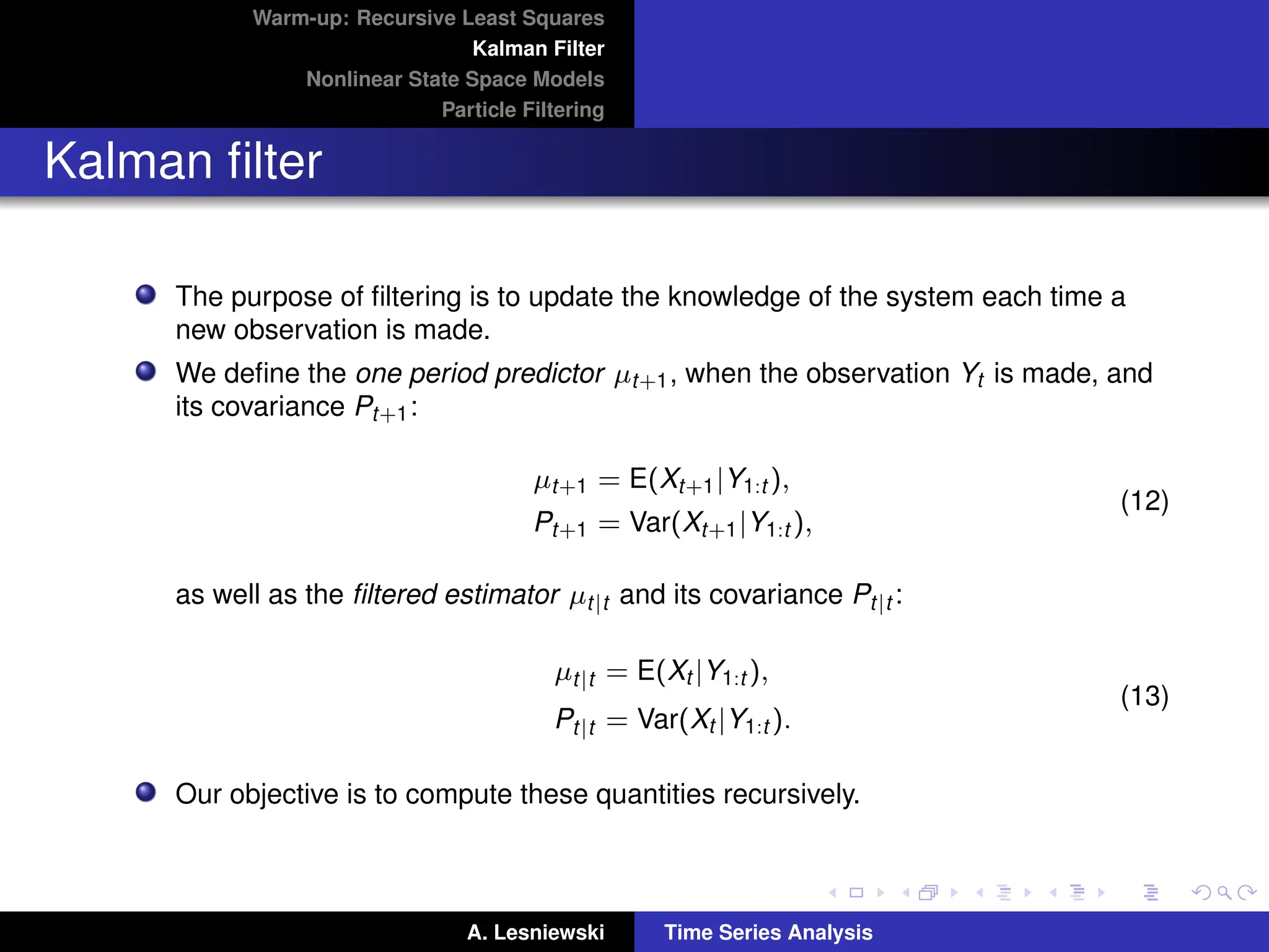
The purpose of filtering is to update the knowledge of the system each time a
new observation is made.
We define the one period predictor µt+1, when the observation Yt is made, and
its covariance Pt+1:
µt+1 = E(Xt+1|Y1:t ),
Pt+1 = Var(Xt+1|Y1:t ),
(12)
as well as the filtered estimator µt|t and its covariance Pt|t :
µt|t = E(Xt |Y1:t ),
Pt|t = Var(Xt |Y1:t ).
(13)
Our objective is to compute these quantities recursively.
A. Lesniewski Time Series Analysis
17.
Warm-up: Recursive LeastSquares
Kalman Filter
Nonlinear State Space Models
Particle Filtering
Kalman filter
We let
vt = Yt − E(Yt |Y1:t−1) (14)
denote the one period prediction error or innovation.
In Homework Assignment #6 we show that vt ’s are mutually independent.
Note that
vt = Yt − E(HXt + ηt |Y1:t−1)
= Yt − Hµt .
As a consequence, we have, for t = 2, 3, . . .,
E(vt |Y1:t−1) = E(HXt + ηt − Hµt |Y1:t−1)
= 0.
(15)
A. Lesniewski Time Series Analysis
18.
Warm-up: Recursive LeastSquares
Kalman Filter
Nonlinear State Space Models
Particle Filtering
Kalman filter
Now we notice that
Var(vt |Y1:t−1) = Var(HXt + ηt − Hµt |Y1:t−1)
= Var(H(Xt − µt )|Y1:t−1) + Var(ηt |Y1:t−1)
= E(H(Xt − µt )(Xt − µt )T
HT
|Y1:t−1) + E(ηt ηT
t |Y1:t−1)
= HPt HT
+ R.
For convenience we denote
Ft = Var(vt |Y1:t−1). (16)
We will assume in the following that the matrix Ft is invertible.
The result of the calculation above can thus be stated as:
Ft = HPt HT
+ R. (17)
This relation allows us to derive a relation between µt and µt|t .
A. Lesniewski Time Series Analysis
19.
Warm-up: Recursive LeastSquares
Kalman Filter
Nonlinear State Space Models
Particle Filtering
Lemma
First, we will establish the following Lemma: Let X and Y be Gaussian jointly
distributed random vectors with
E
X
Y
=
µX
µY
,
and
Var
X
Y
=
ΣXX ΣXY
ΣT
XY ΣYY
Then
E(X|Y) = µX + ΣXY Σ−1
YY
Y − µY
, (18)
and
Var(X|Y) = ΣXX − ΣXY Σ−1
YY
ΣT
XY . (19)
Proof: Consider the random variable
Z = X − ΣXY Σ−1
YY
Y − µY
.
A. Lesniewski Time Series Analysis
20.
Warm-up: Recursive LeastSquares
Kalman Filter
Nonlinear State Space Models
Particle Filtering
Lemma
Since Z is a linear in X and Y, the vector (Y, Z) is Gaussian jointly distributed.
Furthermore,
E(Z) = µX ,
Var(Z) = E((Z − µX )(Z − µX )T
)
= ΣXX − ΣXY Σ−1
YY
ΣT
XY .
Finally,
Cov(Y, Z) = E(Y(Z − µX )T
)
= E(Y(X − µX )T
− Y(Y − µY )T
Σ−1
YY
ΣT
XY )
= 0.
This means that Z and Y are independently distributed!
A. Lesniewski Time Series Analysis
21.
Warm-up: Recursive LeastSquares
Kalman Filter
Nonlinear State Space Models
Particle Filtering
Lemma
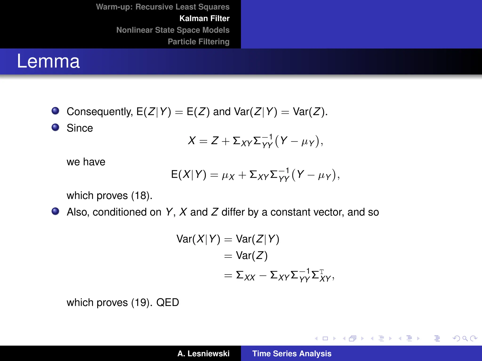
Consequently, E(Z|Y) = E(Z) and Var(Z|Y) = Var(Z).
Since
X = Z + ΣXY Σ−1
YY
Y − µY
,
we have
E(X|Y) = µX + ΣXY Σ−1
YY
Y − µY
,
which proves (18).
Also, conditioned on Y, X and Z differ by a constant vector, and so
Var(X|Y) = Var(Z|Y)
= Var(Z)
= ΣXX − ΣXY Σ−1
YY
ΣT
XY ,
which proves (19). QED
A. Lesniewski Time Series Analysis
22.
Warm-up: Recursive LeastSquares
Kalman Filter
Nonlinear State Space Models
Particle Filtering
Kalman filter
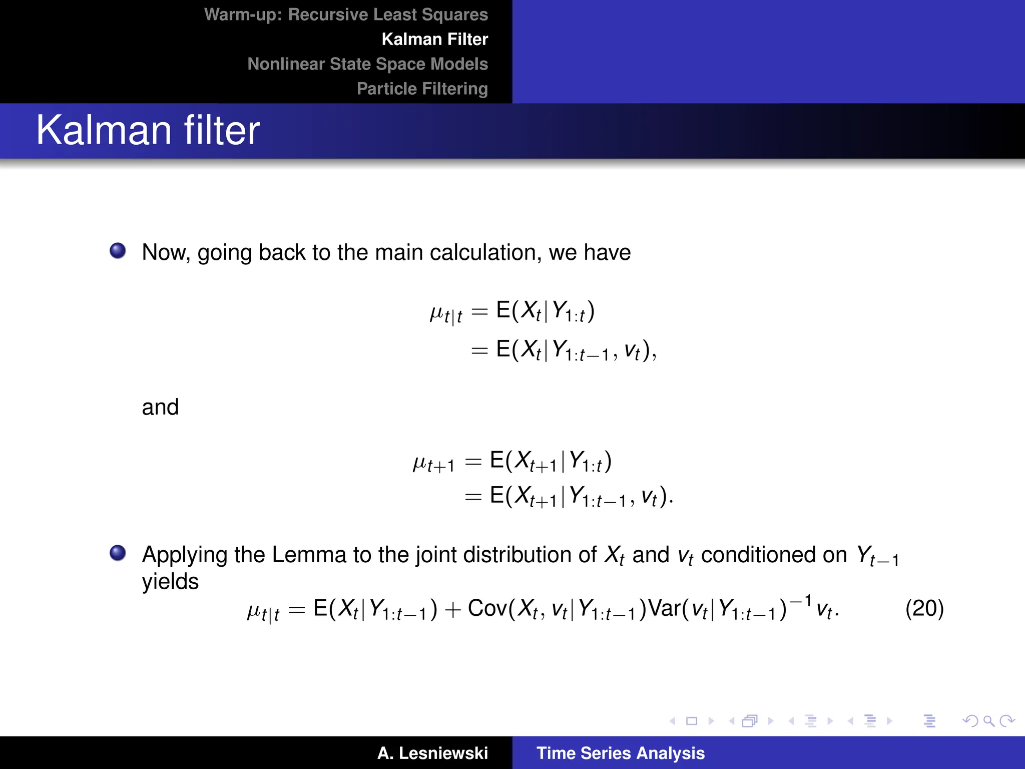
Now, going back to the main calculation, we have
µt|t = E(Xt |Y1:t )
= E(Xt |Y1:t−1, vt ),
and
µt+1 = E(Xt+1|Y1:t )
= E(Xt+1|Y1:t−1, vt ).
Applying the Lemma to the joint distribution of Xt and vt conditioned on Yt−1
yields
µt|t = E(Xt |Y1:t−1) + Cov(Xt , vt |Y1:t−1)Var(vt |Y1:t−1)−1
vt . (20)
A. Lesniewski Time Series Analysis
23.
Warm-up: Recursive LeastSquares
Kalman Filter
Nonlinear State Space Models
Particle Filtering
Kalman filter
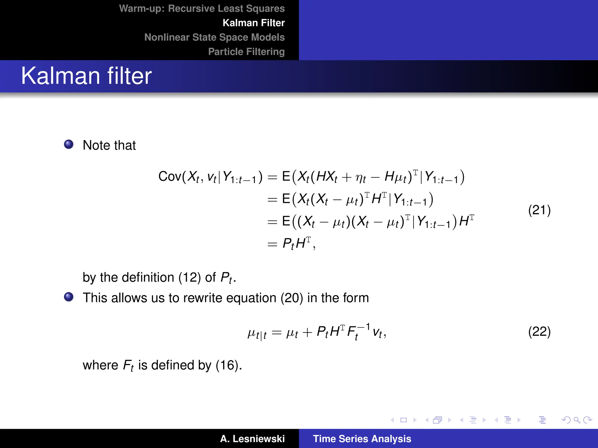
Note that
Cov(Xt , vt |Y1:t−1) = E Xt (HXt + ηt − Hµt )T
|Y1:t−1
= E Xt (Xt − µt )T
HT
|Y1:t−1
= E (Xt − µt )(Xt − µt )T
|Y1:t−1
HT
= Pt HT
,
(21)
by the definition (12) of Pt .
This allows us to rewrite equation (20) in the form
µt|t = µt + Pt HT
F−1
t vt , (22)
where Ft is defined by (16).
A. Lesniewski Time Series Analysis
24.
Warm-up: Recursive LeastSquares
Kalman Filter
Nonlinear State Space Models
Particle Filtering
Kalman filter
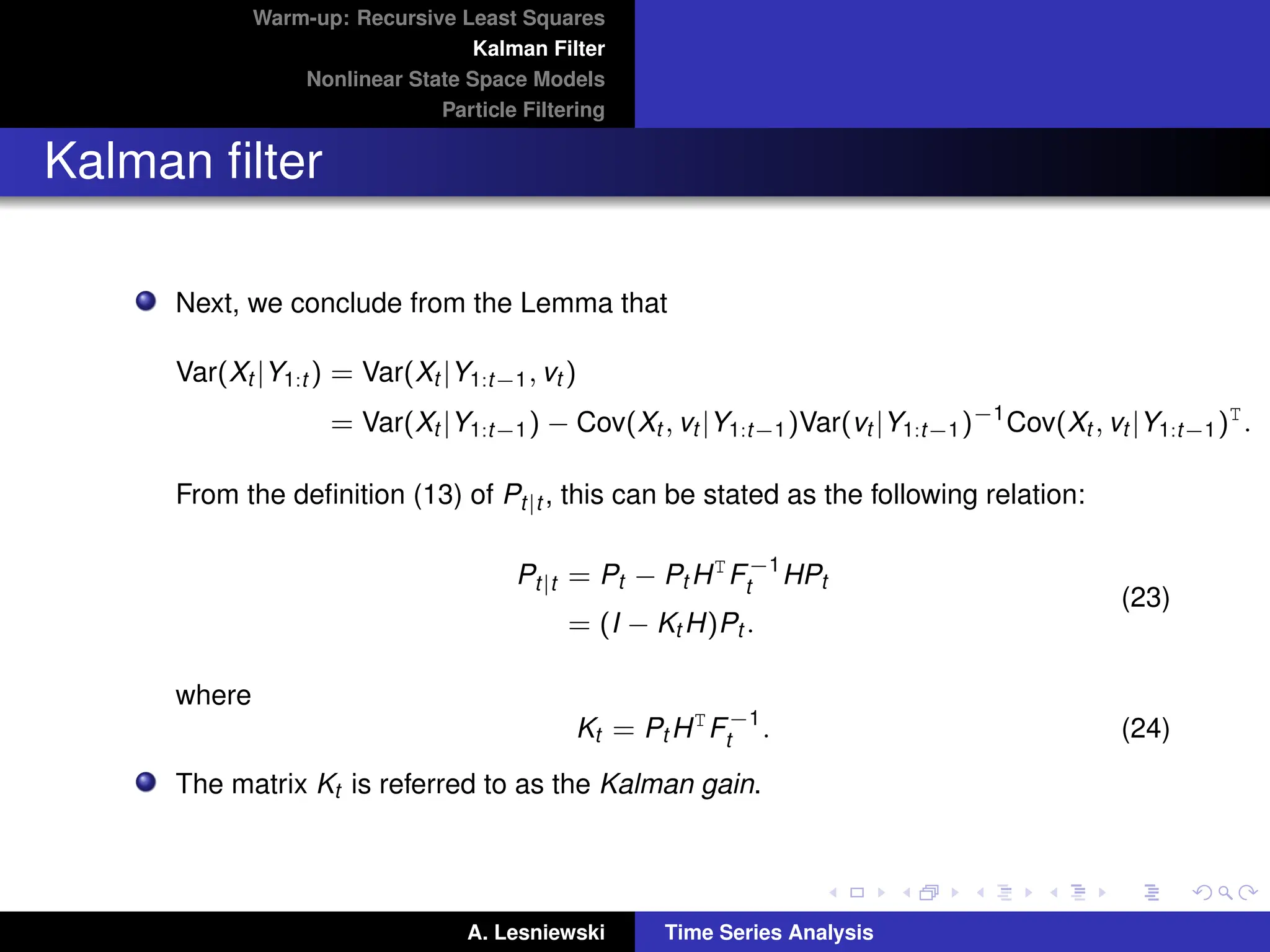
Next, we conclude from the Lemma that
Var(Xt |Y1:t ) = Var(Xt |Y1:t−1, vt )
= Var(Xt |Y1:t−1) − Cov(Xt , vt |Y1:t−1)Var(vt |Y1:t−1)−1
Cov(Xt , vt |Y1:t−1)T
.
From the definition (13) of Pt|t , this can be stated as the following relation:
Pt|t = Pt − Pt HT
F−1
t HPt
= (I − Kt H)Pt .
(23)
where
Kt = Pt HT
F−1
t . (24)
The matrix Kt is referred to as the Kalman gain.
A. Lesniewski Time Series Analysis
25.
Warm-up: Recursive LeastSquares
Kalman Filter
Nonlinear State Space Models
Particle Filtering
Kalman filter
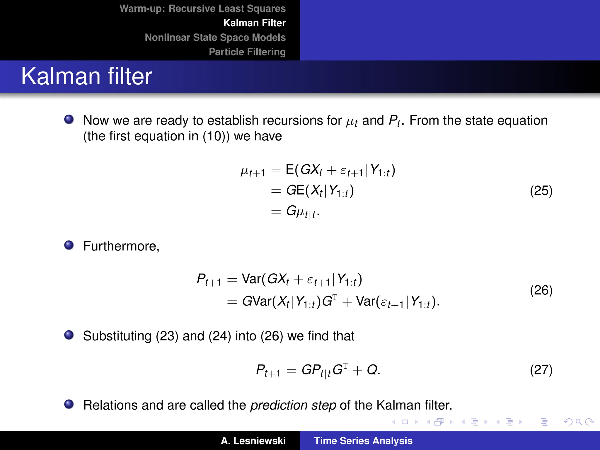
Now we are ready to establish recursions for µt and Pt . From the state equation
(the first equation in (10)) we have
µt+1 = E(GXt + εt+1|Y1:t )
= GE(Xt |Y1:t )
= Gµt|t .
(25)
Furthermore,
Pt+1 = Var(GXt + εt+1|Y1:t )
= GVar(Xt |Y1:t )GT
+ Var(εt+1|Y1:t ).
(26)
Substituting (23) and (24) into (26) we find that
Pt+1 = GPt|t GT
+ Q. (27)
Relations and are called the prediction step of the Kalman filter.
A. Lesniewski Time Series Analysis
26.
Warm-up: Recursive LeastSquares
Kalman Filter
Nonlinear State Space Models
Particle Filtering
Kalman filter
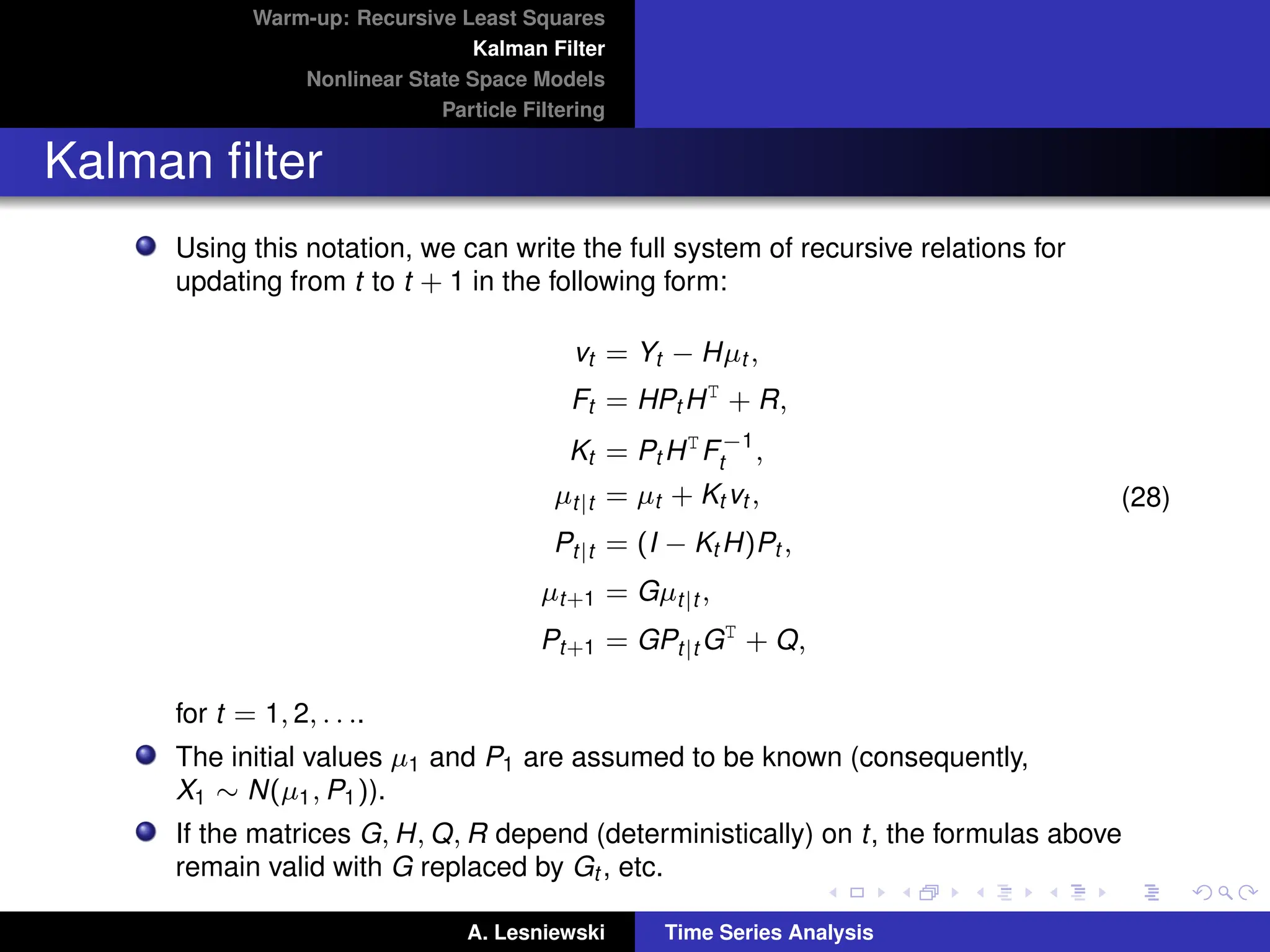
Using this notation, we can write the full system of recursive relations for
updating from t to t + 1 in the following form:
vt = Yt − Hµt ,
Ft = HPt HT
+ R,
Kt = Pt HT
F−1
t ,
µt|t = µt + Kt vt ,
Pt|t = (I − Kt H)Pt ,
µt+1 = Gµt|t ,
Pt+1 = GPt|t GT
+ Q,
(28)
for t = 1, 2, . . ..
The initial values µ1 and P1 are assumed to be known (consequently,
X1 ∼ N(µ1, P1)).
If the matrices G, H, Q, R depend (deterministically) on t, the formulas above
remain valid with G replaced by Gt , etc.
A. Lesniewski Time Series Analysis
27.
Warm-up: Recursive LeastSquares
Kalman Filter
Nonlinear State Space Models
Particle Filtering
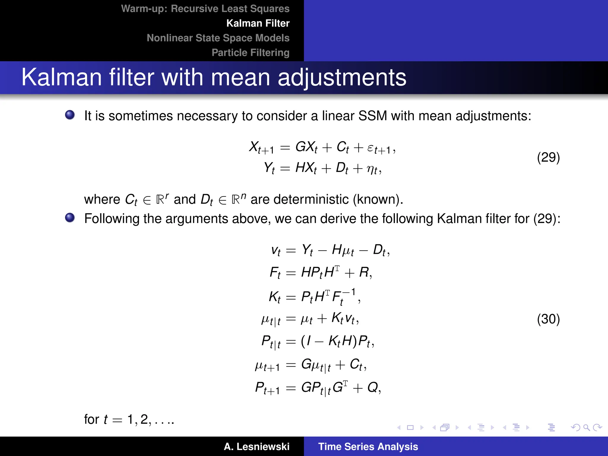
Kalman filter with mean adjustments
It is sometimes necessary to consider a linear SSM with mean adjustments:
Xt+1 = GXt + Ct + εt+1,
Yt = HXt + Dt + ηt ,
(29)
where Ct ∈ Rr and Dt ∈ Rn are deterministic (known).
Following the arguments above, we can derive the following Kalman filter for (29):
vt = Yt − Hµt − Dt ,
Ft = HPt HT
+ R,
Kt = Pt HT
F−1
t ,
µt|t = µt + Kt vt ,
Pt|t = (I − Kt H)Pt ,
µt+1 = Gµt|t + Ct ,
Pt+1 = GPt|t GT
+ Q,
(30)
for t = 1, 2, . . ..
A. Lesniewski Time Series Analysis
28.
Warm-up: Recursive LeastSquares
Kalman Filter
Nonlinear State Space Models
Particle Filtering
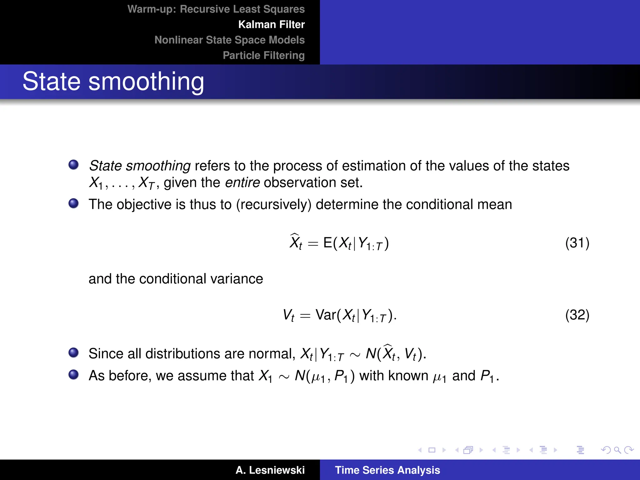
State smoothing
State smoothing refers to the process of estimation of the values of the states
X1, . . . , XT , given the entire observation set.
The objective is thus to (recursively) determine the conditional mean
b
Xt = E(Xt |Y1:T ) (31)
and the conditional variance
Vt = Var(Xt |Y1:T ). (32)
Since all distributions are normal, Xt |Y1:T ∼ N(b
Xt , Vt ).
As before, we assume that X1 ∼ N(µ1, P1) with known µ1 and P1.
A. Lesniewski Time Series Analysis
29.
Warm-up: Recursive LeastSquares
Kalman Filter
Nonlinear State Space Models
Particle Filtering
State smoothing
An analysis, similar to the derivation of the Kalman filter leads to the following
result (see [2]) for the derivation).
The smoothing process consists of two phases:
(i) forward sweep of the Kalman filter (28) for t = 1, . . . , T,
(ii) backward recursion
Rt−1 = HT
F−1
t vt + LT
t rt ,
Nt−1 = HT
F−1
t H + LT
t Nt Lt ,
b
Xt = µt + Pt Rt−1,
Vt = Pt − Pt Nt−1Pt ,
(33)
where Lt = G(I − Kt H), for t = T, T − 1, . . ., with the terminal condition
RT = 0 and NT = 0.
This version of the smoothing algorithm is somewhat unintuitive but
computationally efficient.
A. Lesniewski Time Series Analysis
30.
Warm-up: Recursive LeastSquares
Kalman Filter
Nonlinear State Space Models
Particle Filtering
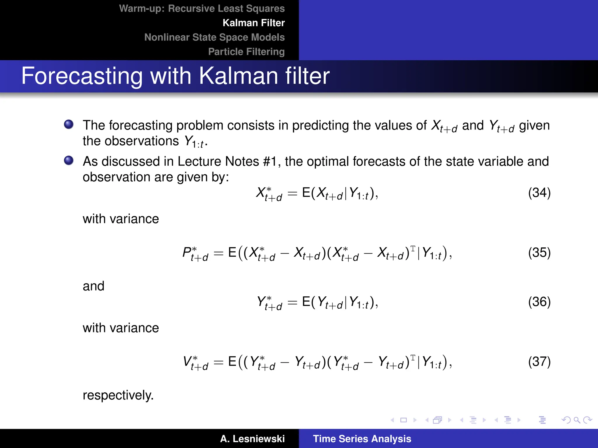
Forecasting with Kalman filter
The forecasting problem consists in predicting the values of Xt+d and Yt+d given
the observations Y1:t .
As discussed in Lecture Notes #1, the optimal forecasts of the state variable and
observation are given by:
X∗
t+d = E(Xt+d |Y1:t ), (34)
with variance
P∗
t+d = E (X∗
t+d − Xt+d )(X∗
t+d − Xt+d )T
|Y1:t
, (35)
and
Y∗
t+d = E(Yt+d |Y1:t ), (36)
with variance
V∗
t+d = E (Y∗
t+d − Yt+d )(Y∗
t+d − Yt+d )T
|Y1:t
, (37)
respectively.
A. Lesniewski Time Series Analysis
31.
Warm-up: Recursive LeastSquares
Kalman Filter
Nonlinear State Space Models
Particle Filtering
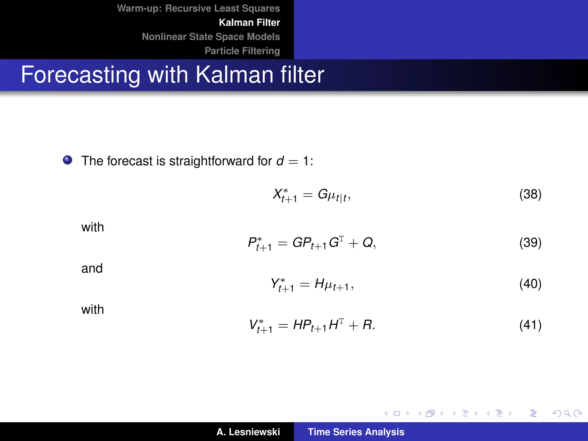
Forecasting with Kalman filter
The forecast is straightforward for d = 1:
X∗
t+1 = Gµt|t , (38)
with
P∗
t+1 = GPt+1GT
+ Q, (39)
and
Y∗
t+1 = Hµt+1, (40)
with
V∗
t+1 = HPt+1HT
+ R. (41)
A. Lesniewski Time Series Analysis
32.
Warm-up: Recursive LeastSquares
Kalman Filter
Nonlinear State Space Models
Particle Filtering
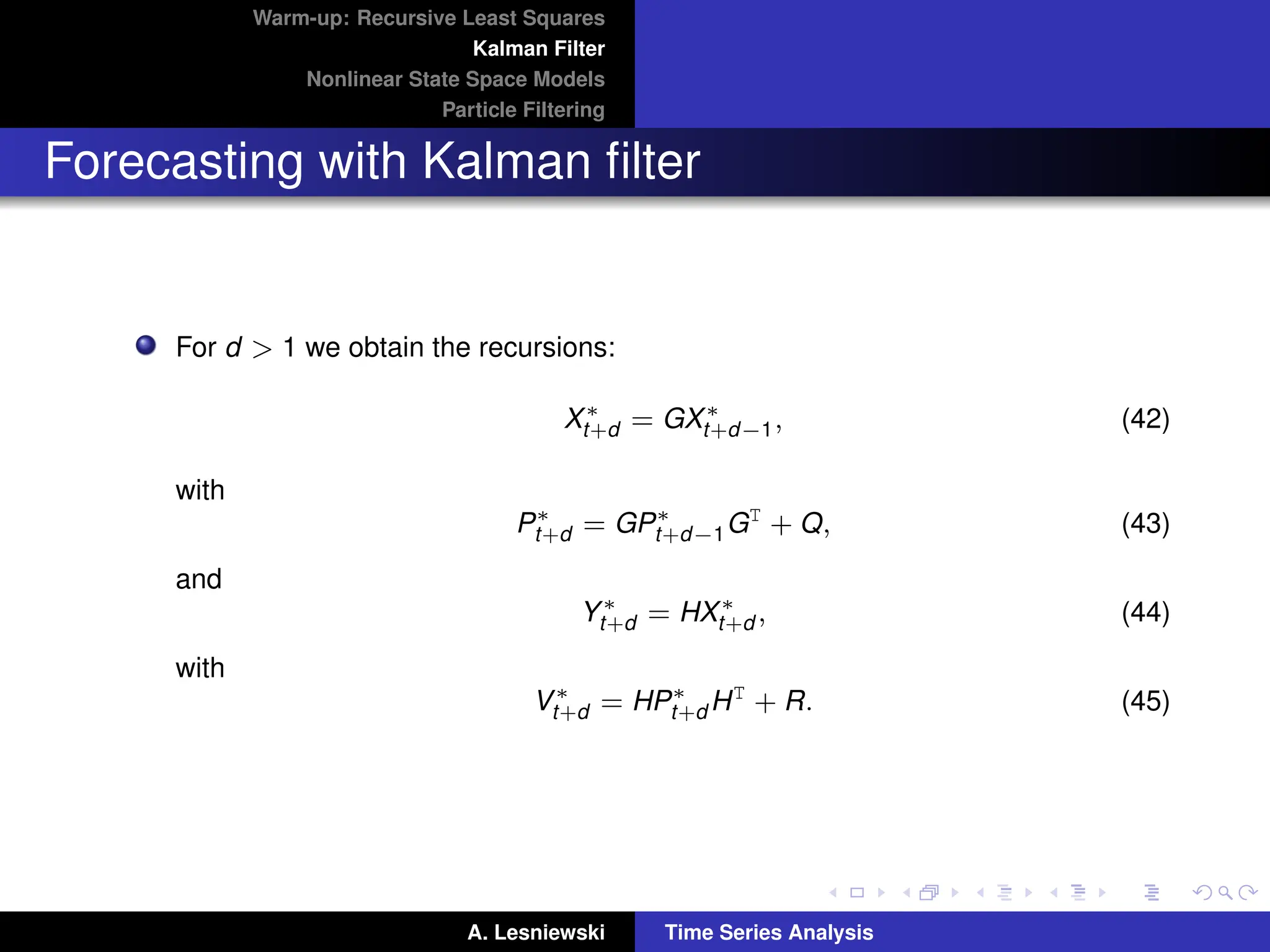
Forecasting with Kalman filter
For d 1 we obtain the recursions:
X∗
t+d = GX∗
t+d−1, (42)
with
P∗
t+d = GP∗
t+d−1GT
+ Q, (43)
and
Y∗
t+d = HX∗
t+d , (44)
with
V∗
t+d = HP∗
t+d HT
+ R. (45)
A. Lesniewski Time Series Analysis
33.
Warm-up: Recursive LeastSquares
Kalman Filter
Nonlinear State Space Models
Particle Filtering
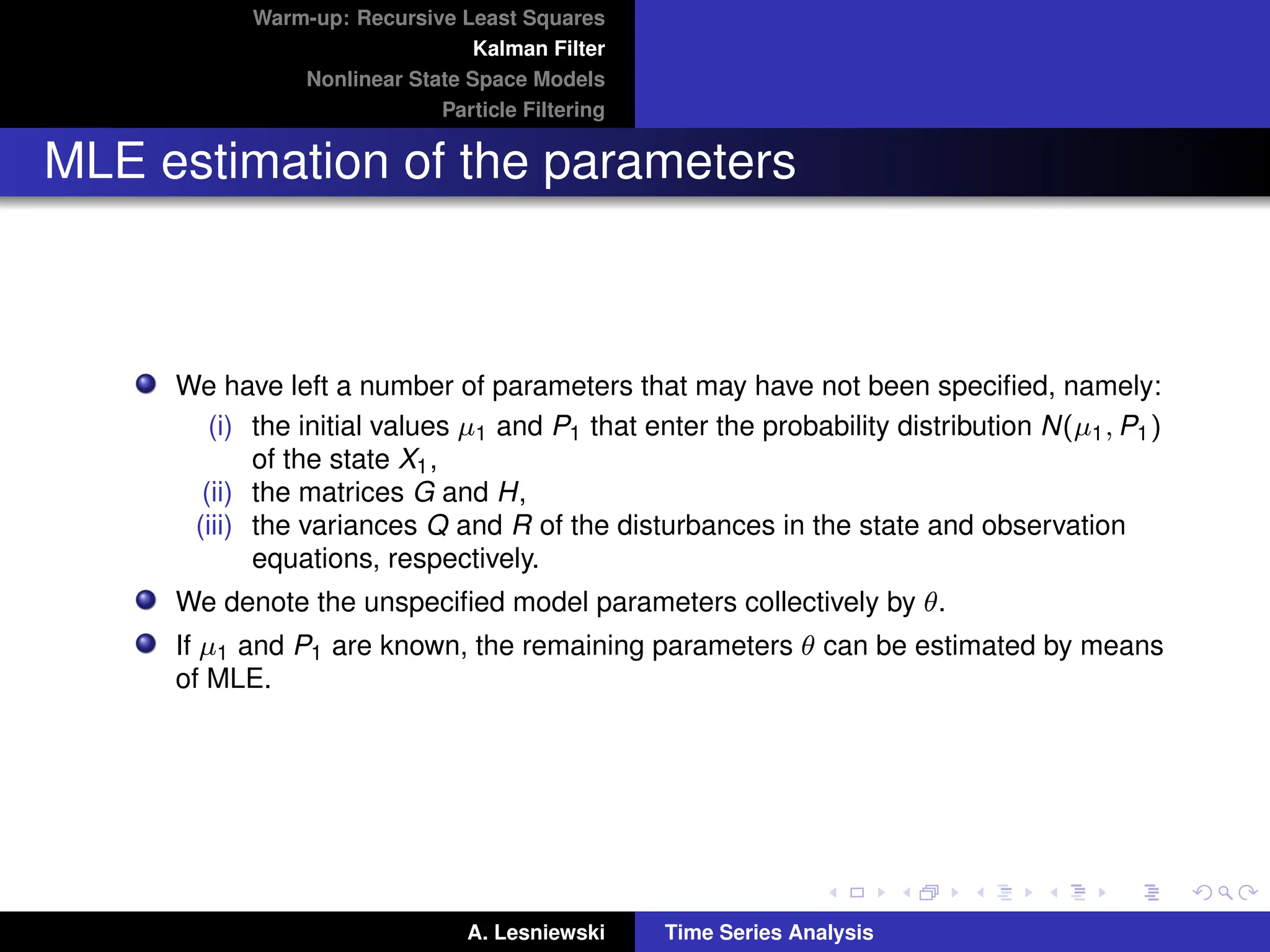
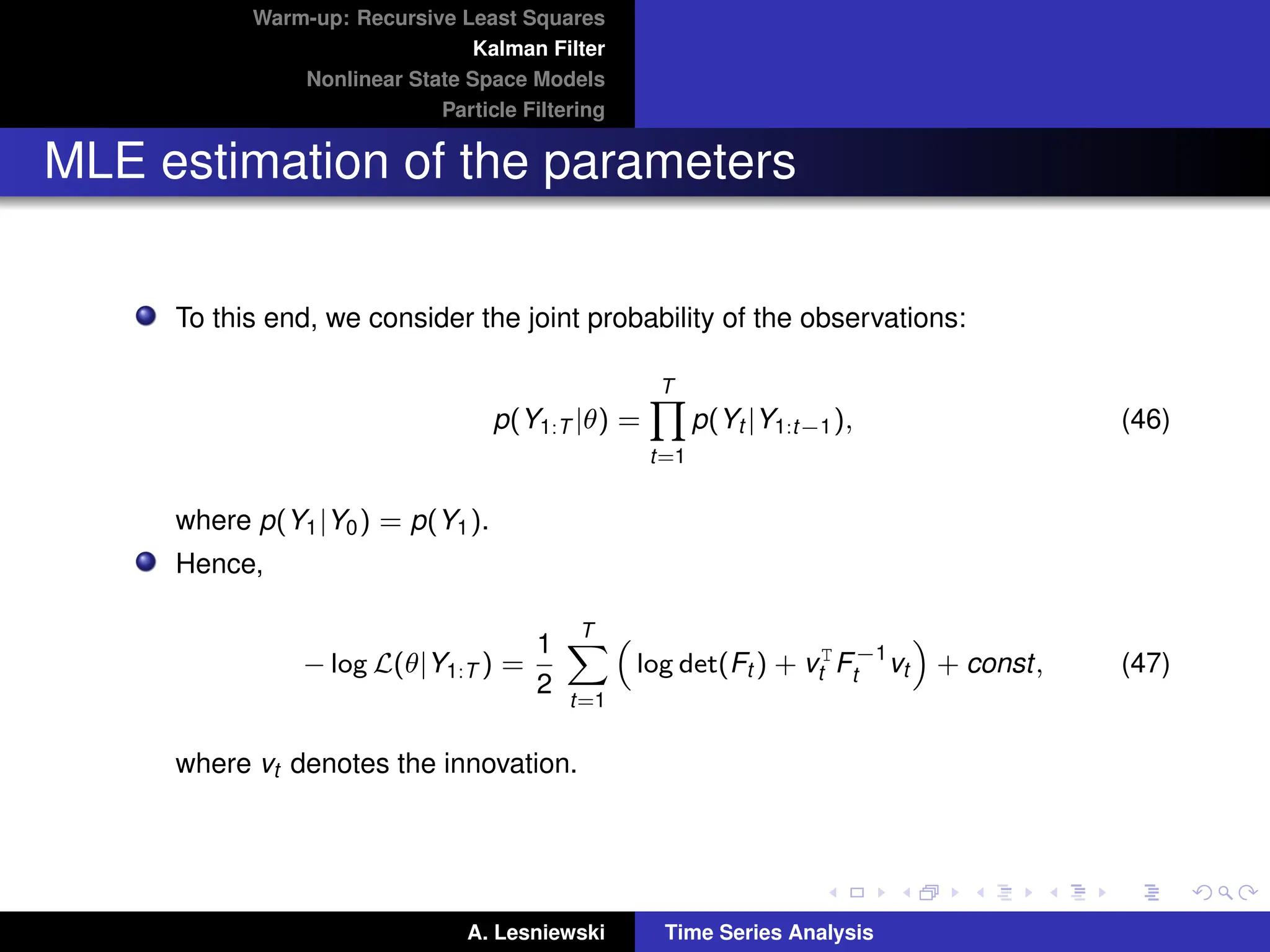
MLE estimation of the parameters
We have left a number of parameters that may have not been specified, namely:
(i) the initial values µ1 and P1 that enter the probability distribution N(µ1, P1)
of the state X1,
(ii) the matrices G and H,
(iii) the variances Q and R of the disturbances in the state and observation
equations, respectively.
We denote the unspecified model parameters collectively by θ.
If µ1 and P1 are known, the remaining parameters θ can be estimated by means
of MLE.
A. Lesniewski Time Series Analysis
34.
Warm-up: Recursive LeastSquares
Kalman Filter
Nonlinear State Space Models
Particle Filtering
MLE estimation of the parameters
To this end, we consider the joint probability of the observations:
p(Y1:T |θ) =
T
Y
t=1
p(Yt |Y1:t−1), (46)
where p(Y1|Y0) = p(Y1).
Hence,
− log L(θ|Y1:T ) =
1
2
T
X
t=1
log det(Ft ) + vT
t F−1
t vt
+ const, (47)
where vt denotes the innovation.
A. Lesniewski Time Series Analysis
35.
Warm-up: Recursive LeastSquares
Kalman Filter
Nonlinear State Space Models
Particle Filtering
MLE estimation of the parameters
For each t, the value of the log likelihood function is calculated by running the
Kalman filter.
Searching for the minimum of this log likelihood function using an efficient
algorithm such as BFGS, we find estimates of θ.
In the case of unknown µ1 and P1, one can use the diffuse log likelihood
method, which is discussed in detail in [2].
Alternatively, one can regard µ1 and P1 hyperparameters of the model.
A. Lesniewski Time Series Analysis
36.
Warm-up: Recursive LeastSquares
Kalman Filter
Nonlinear State Space Models
Particle Filtering
Nonlinear state space models
The recursion relations defining the Kalman filter can be extended to the case of
more general state space models.
Some of these extensions are straightforward (such as adding constant terms to
the right hand sides of the state and observation equations in (10)), others are
fundamentally more complicated.
In the remainder of this lecture we summarize these extensions following [2].
A. Lesniewski Time Series Analysis
37.
Warm-up: Recursive LeastSquares
Kalman Filter
Nonlinear State Space Models
Particle Filtering
Nonlinear state space models
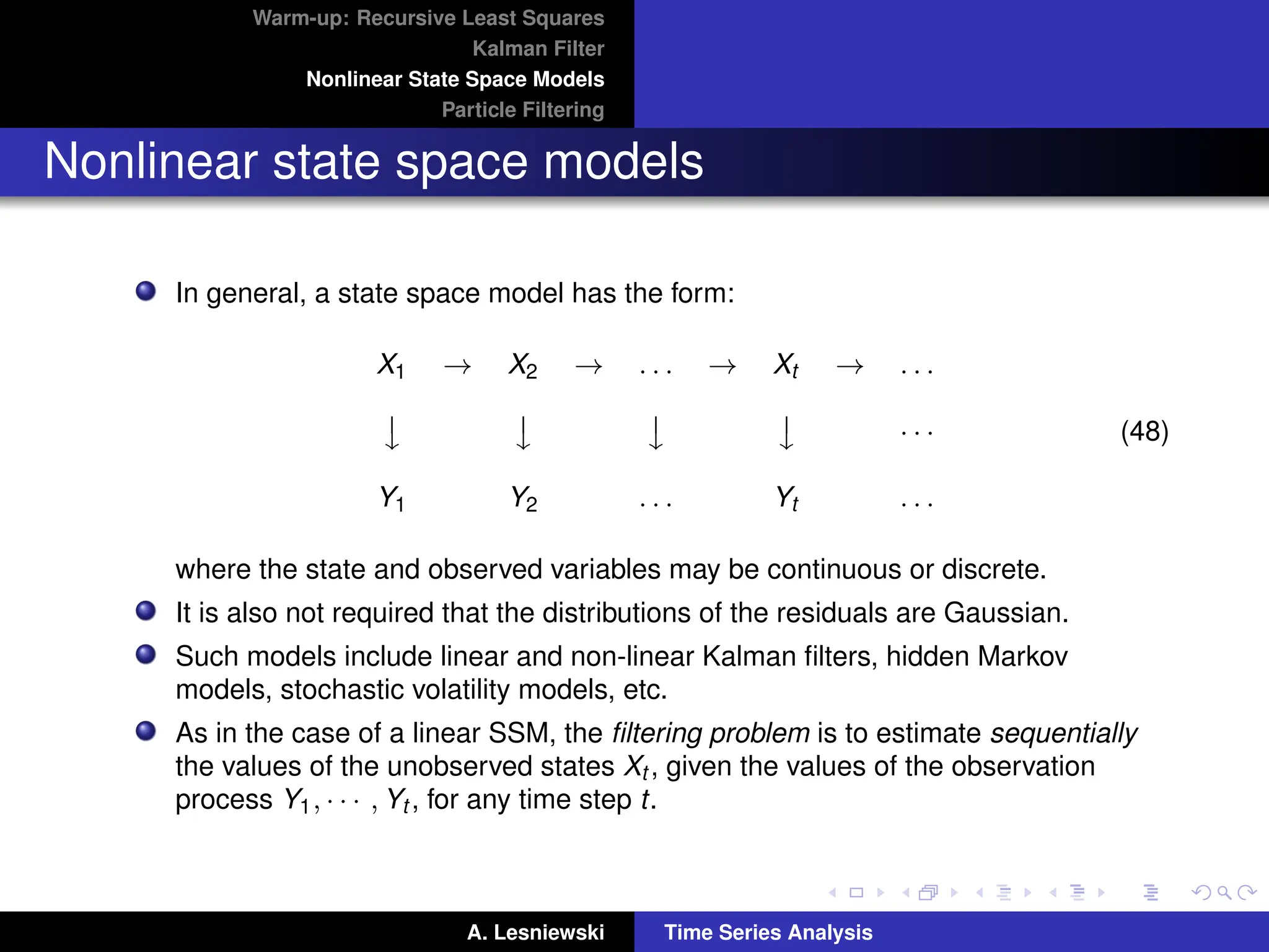
In general, a state space model has the form:
X1 → X2 → . . . → Xt → . . .
y
y
y
y · · ·
Y1 Y2 . . . Yt . . .
(48)
where the state and observed variables may be continuous or discrete.
It is also not required that the distributions of the residuals are Gaussian.
Such models include linear and non-linear Kalman filters, hidden Markov
models, stochastic volatility models, etc.
As in the case of a linear SSM, the filtering problem is to estimate sequentially
the values of the unobserved states Xt , given the values of the observation
process Y1, · · · , Yt , for any time step t.
A. Lesniewski Time Series Analysis
38.
Warm-up: Recursive LeastSquares
Kalman Filter
Nonlinear State Space Models
Particle Filtering
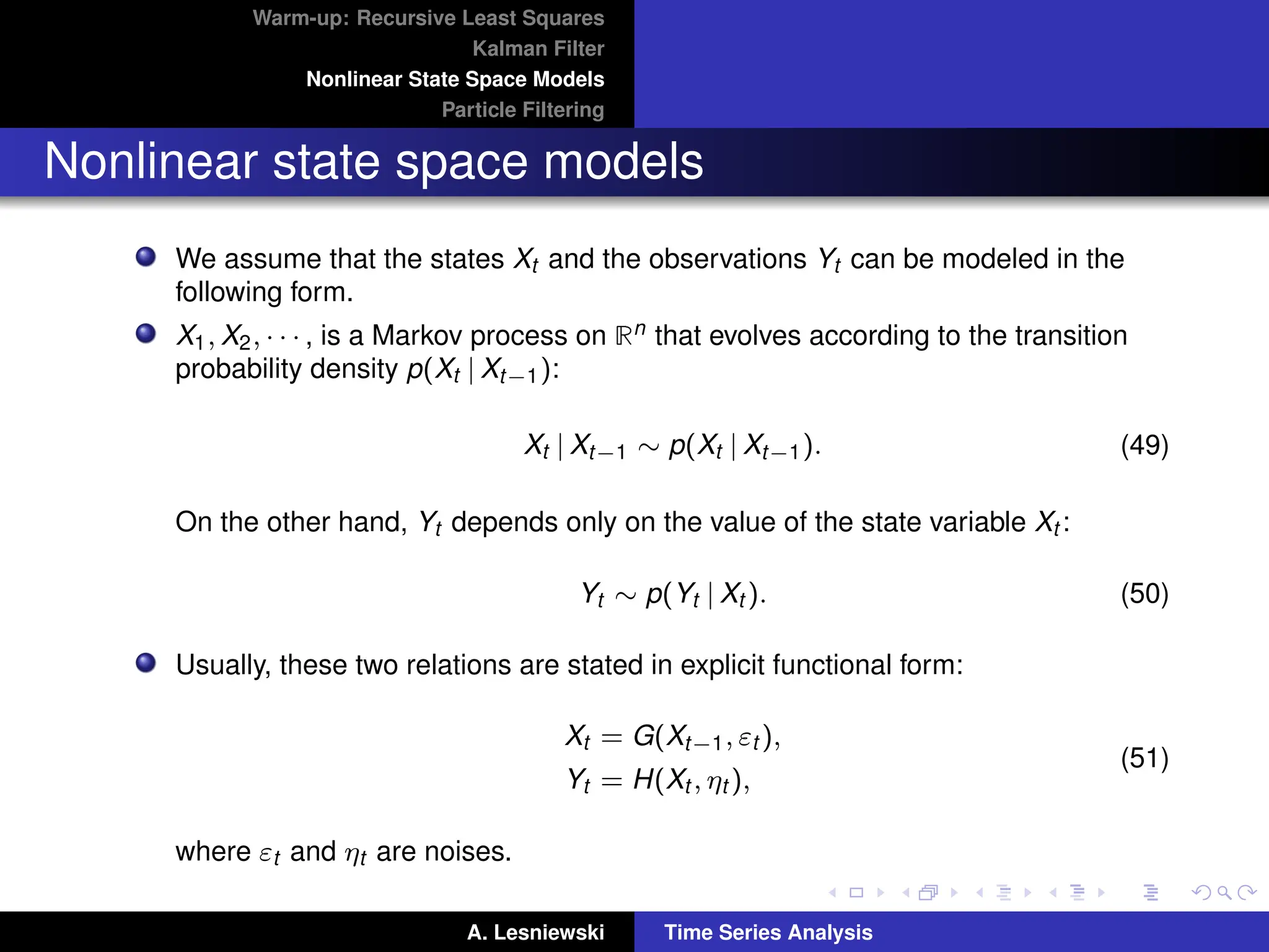
Nonlinear state space models
We assume that the states Xt and the observations Yt can be modeled in the
following form.
X1, X2, · · · , is a Markov process on Rn that evolves according to the transition
probability density p(Xt | Xt−1):
Xt | Xt−1 ∼ p(Xt | Xt−1). (49)
On the other hand, Yt depends only on the value of the state variable Xt :
Yt ∼ p(Yt | Xt ). (50)
Usually, these two relations are stated in explicit functional form:
Xt = G(Xt−1, εt ),
Yt = H(Xt , ηt ),
(51)
where εt and ηt are noises.
A. Lesniewski Time Series Analysis
39.
Warm-up: Recursive LeastSquares
Kalman Filter
Nonlinear State Space Models
Particle Filtering
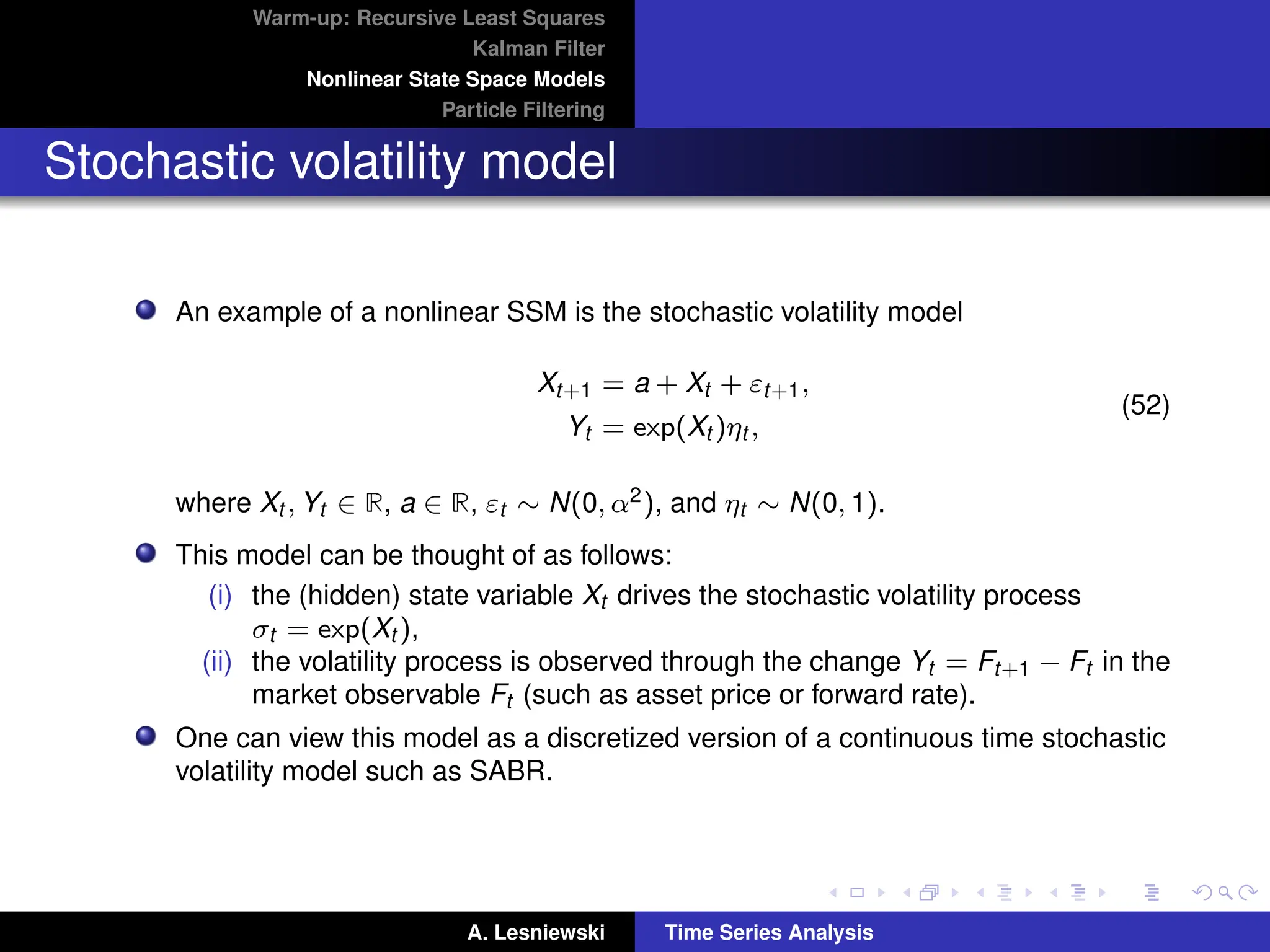
Stochastic volatility model
An example of a nonlinear SSM is the stochastic volatility model
Xt+1 = a + Xt + εt+1,
Yt = exp(Xt )ηt ,
(52)
where Xt , Yt ∈ R, a ∈ R, εt ∼ N(0, α2), and ηt ∼ N(0, 1).
This model can be thought of as follows:
(i) the (hidden) state variable Xt drives the stochastic volatility process
σt = exp(Xt ),
(ii) the volatility process is observed through the change Yt = Ft+1 − Ft in the
market observable Ft (such as asset price or forward rate).
One can view this model as a discretized version of a continuous time stochastic
volatility model such as SABR.
A. Lesniewski Time Series Analysis
40.
Warm-up: Recursive LeastSquares
Kalman Filter
Nonlinear State Space Models
Particle Filtering
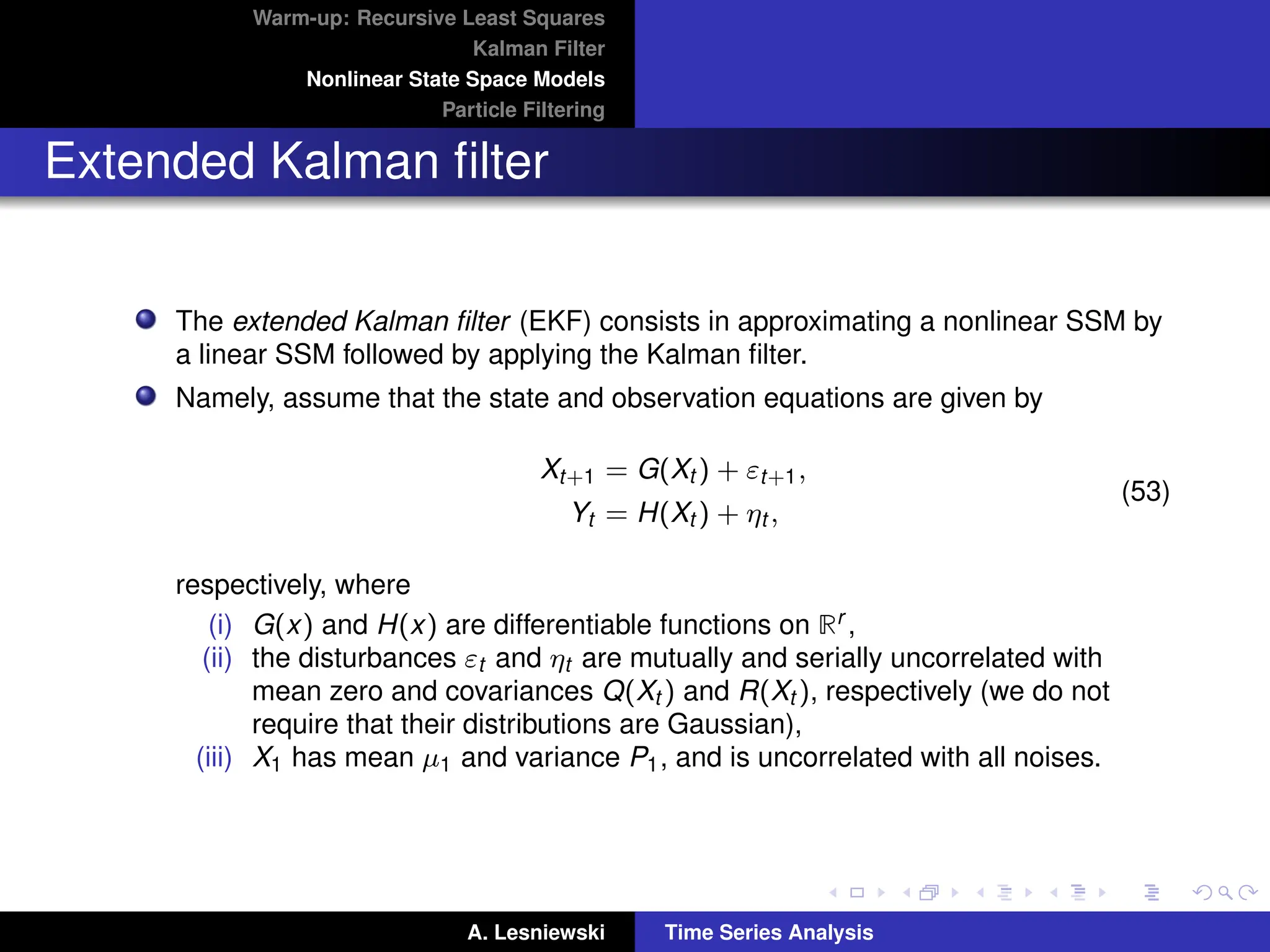
Extended Kalman filter
The extended Kalman filter (EKF) consists in approximating a nonlinear SSM by
a linear SSM followed by applying the Kalman filter.
Namely, assume that the state and observation equations are given by
Xt+1 = G(Xt ) + εt+1,
Yt = H(Xt ) + ηt ,
(53)
respectively, where
(i) G(x) and H(x) are differentiable functions on Rr ,
(ii) the disturbances εt and ηt are mutually and serially uncorrelated with
mean zero and covariances Q(Xt ) and R(Xt ), respectively (we do not
require that their distributions are Gaussian),
(iii) X1 has mean µ1 and variance P1, and is uncorrelated with all noises.
A. Lesniewski Time Series Analysis
41.
Warm-up: Recursive LeastSquares
Kalman Filter
Nonlinear State Space Models
Particle Filtering
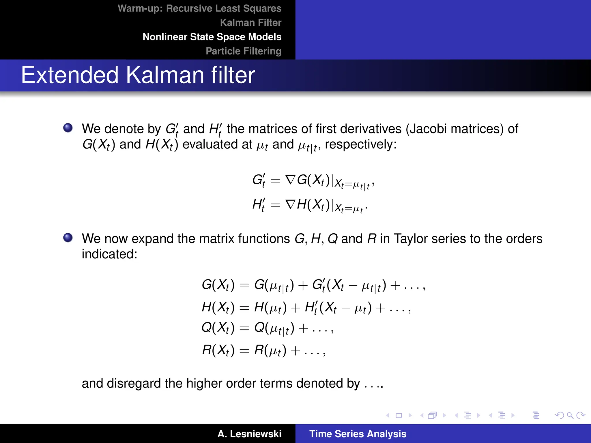
Extended Kalman filter
We denote by G0
t and H0
t the matrices of first derivatives (Jacobi matrices) of
G(Xt ) and H(Xt ) evaluated at µt and µt|t , respectively:
G0
t = ∇G(Xt )|Xt =µt|t
,
H0
t = ∇H(Xt )|Xt =µt
.
We now expand the matrix functions G, H, Q and R in Taylor series to the orders
indicated:
G(Xt ) = G(µt|t ) + G0
t (Xt − µt|t ) + . . . ,
H(Xt ) = H(µt ) + H0
t (Xt − µt ) + . . . ,
Q(Xt ) = Q(µt|t ) + . . . ,
R(Xt ) = R(µt ) + . . . ,
and disregard the higher order terms denoted by . . ..
A. Lesniewski Time Series Analysis
42.
Warm-up: Recursive LeastSquares
Kalman Filter
Nonlinear State Space Models
Particle Filtering
Extended Kalman filter
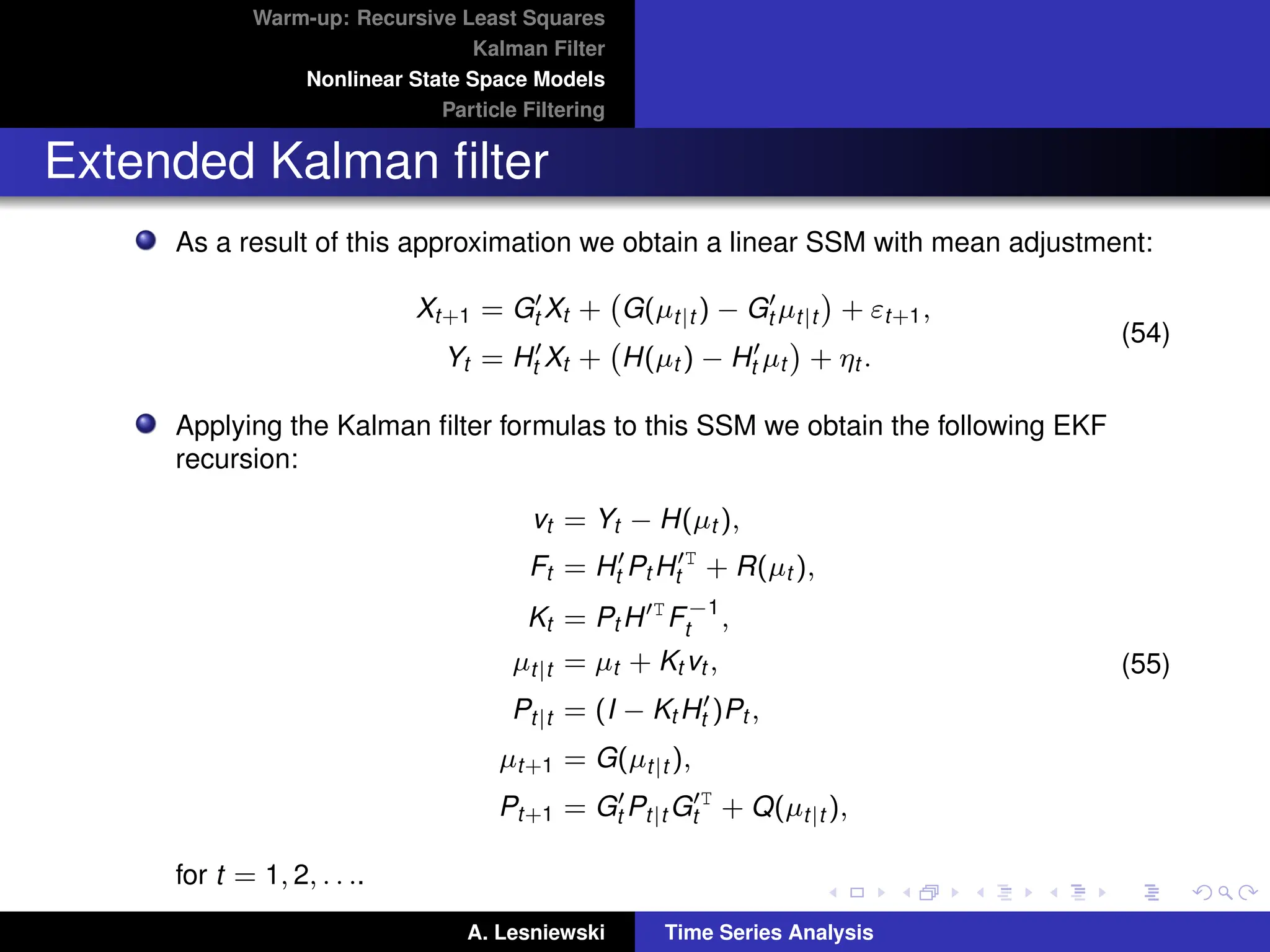
As a result of this approximation we obtain a linear SSM with mean adjustment:
Xt+1 = G0
t Xt + G(µt|t ) − G0
t µt|t
+ εt+1,
Yt = H0
t Xt + H(µt ) − H0
t µt
+ ηt .
(54)
Applying the Kalman filter formulas to this SSM we obtain the following EKF
recursion:
vt = Yt − H(µt ),
Ft = H0
t Pt H0T
t + R(µt ),
Kt = Pt H0T
F−1
t ,
µt|t = µt + Kt vt ,
Pt|t = (I − Kt H0
t )Pt ,
µt+1 = G(µt|t ),
Pt+1 = G0
t Pt|t G0T
t + Q(µt|t ),
(55)
for t = 1, 2, . . ..
A. Lesniewski Time Series Analysis
43.
Warm-up: Recursive LeastSquares
Kalman Filter
Nonlinear State Space Models
Particle Filtering
Extended Kalman filter
The EKF works well if the functions G and H are weakly nonlinear, for strongly
nonlinear models its performance may be poor.
Other extensions of the Kalman filter have been developed, including the
unscented Kalman filter (UKF).
It is based on a different principle than the EKF: rather than approximating G and
H by linear expressions, one matches approximately the first and second
moments of a nonlinear function of a Gaussian random variable, see [2] for
details.
Another approach to inference in nonlinear SSMs is via Monte Carlo (MC)
techniques particle filters, a.k.a. sequential Monte Carlo.
A. Lesniewski Time Series Analysis
44.
Warm-up: Recursive LeastSquares
Kalman Filter
Nonlinear State Space Models
Particle Filtering
Particle filtering
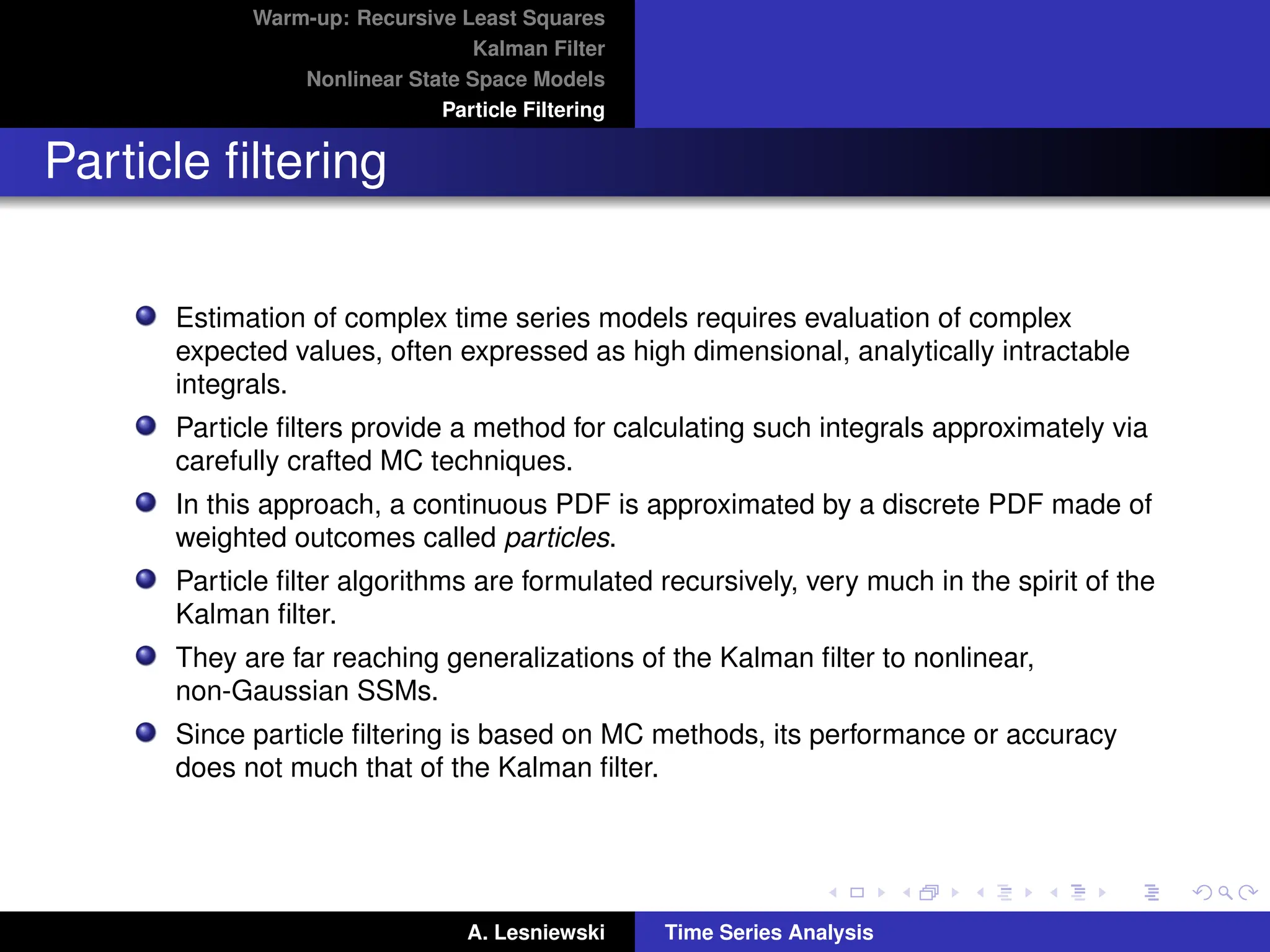
Estimation of complex time series models requires evaluation of complex
expected values, often expressed as high dimensional, analytically intractable
integrals.
Particle filters provide a method for calculating such integrals approximately via
carefully crafted MC techniques.
In this approach, a continuous PDF is approximated by a discrete PDF made of
weighted outcomes called particles.
Particle filter algorithms are formulated recursively, very much in the spirit of the
Kalman filter.
They are far reaching generalizations of the Kalman filter to nonlinear,
non-Gaussian SSMs.
Since particle filtering is based on MC methods, its performance or accuracy
does not much that of the Kalman filter.
A. Lesniewski Time Series Analysis
45.
Warm-up: Recursive LeastSquares
Kalman Filter
Nonlinear State Space Models
Particle Filtering
Nonlinear state space models
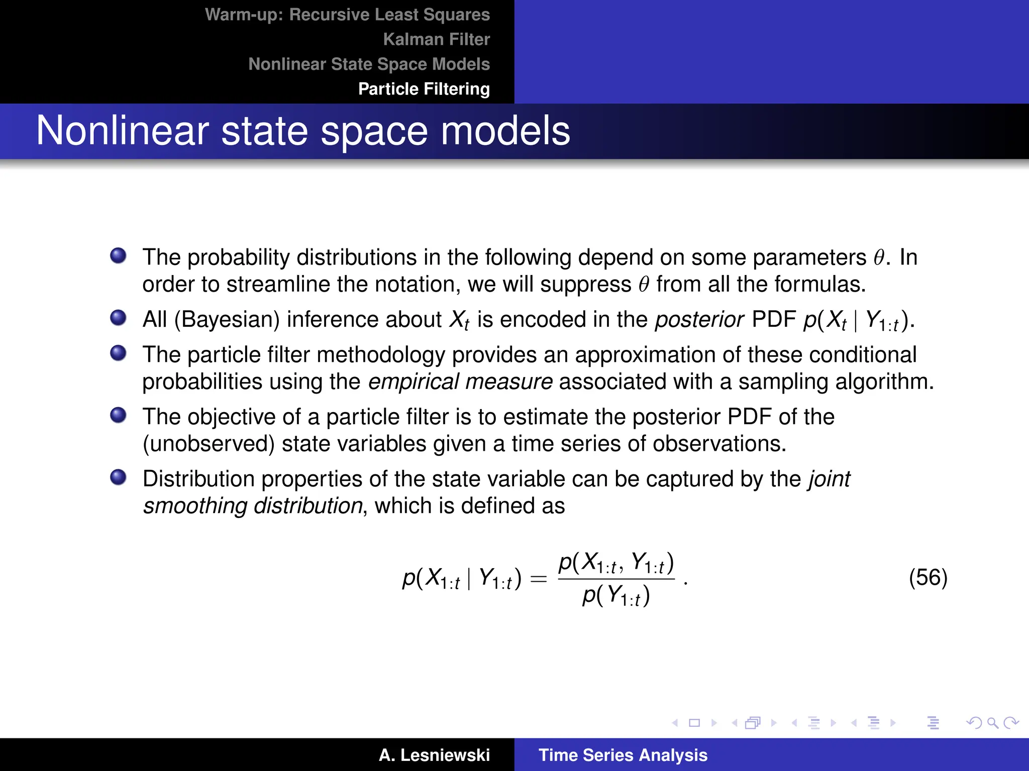
The probability distributions in the following depend on some parameters θ. In
order to streamline the notation, we will suppress θ from all the formulas.
All (Bayesian) inference about Xt is encoded in the posterior PDF p(Xt | Y1:t ).
The particle filter methodology provides an approximation of these conditional
probabilities using the empirical measure associated with a sampling algorithm.
The objective of a particle filter is to estimate the posterior PDF of the
(unobserved) state variables given a time series of observations.
Distribution properties of the state variable can be captured by the joint
smoothing distribution, which is defined as
p(X1:t | Y1:t ) =
p(X1:t , Y1:t )
p(Y1:t )
. (56)
A. Lesniewski Time Series Analysis
46.
Warm-up: Recursive LeastSquares
Kalman Filter
Nonlinear State Space Models
Particle Filtering
Joint smoothing distribution
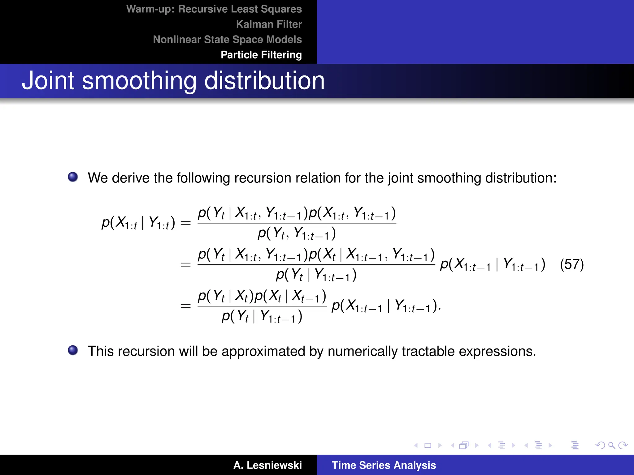
We derive the following recursion relation for the joint smoothing distribution:
p(X1:t | Y1:t ) =
p(Yt | X1:t , Y1:t−1)p(X1:t , Y1:t−1)
p(Yt , Y1:t−1)
=
p(Yt | X1:t , Y1:t−1)p(Xt | X1:t−1, Y1:t−1)
p(Yt | Y1:t−1)
p(X1:t−1 | Y1:t−1)
=
p(Yt | Xt )p(Xt | Xt−1)
p(Yt | Y1:t−1)
p(X1:t−1 | Y1:t−1).
(57)
This recursion will be approximated by numerically tractable expressions.
A. Lesniewski Time Series Analysis
47.
Warm-up: Recursive LeastSquares
Kalman Filter
Nonlinear State Space Models
Particle Filtering
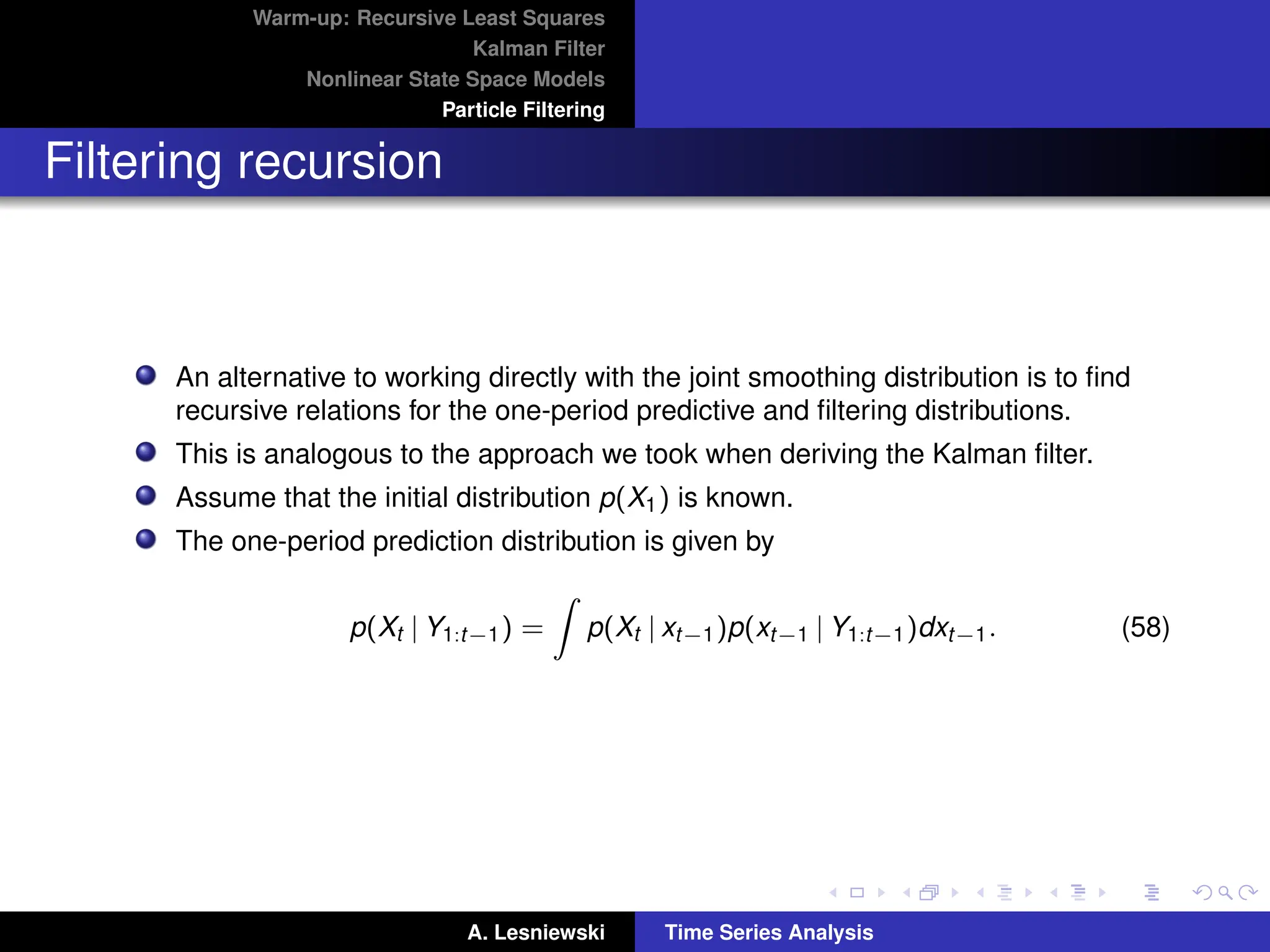
Filtering recursion
An alternative to working directly with the joint smoothing distribution is to find
recursive relations for the one-period predictive and filtering distributions.
This is analogous to the approach we took when deriving the Kalman filter.
Assume that the initial distribution p(X1) is known.
The one-period prediction distribution is given by
p(Xt | Y1:t−1) =
Z
p(Xt | xt−1)p(xt−1 | Y1:t−1)dxt−1. (58)
A. Lesniewski Time Series Analysis
48.
Warm-up: Recursive LeastSquares
Kalman Filter
Nonlinear State Space Models
Particle Filtering
Filtering recursion
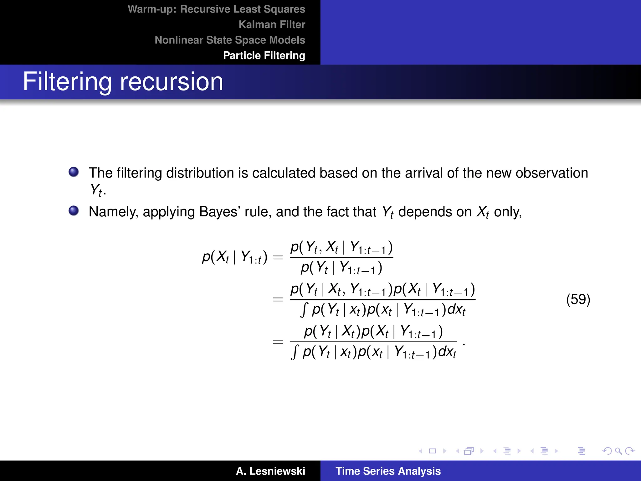
The filtering distribution is calculated based on the arrival of the new observation
Yt .
Namely, applying Bayes’ rule, and the fact that Yt depends on Xt only,
p(Xt | Y1:t ) =
p(Yt , Xt | Y1:t−1)
p(Yt | Y1:t−1)
=
p(Yt | Xt , Y1:t−1)p(Xt | Y1:t−1)
R
p(Yt | xt )p(xt | Y1:t−1)dxt
=
p(Yt | Xt )p(Xt | Y1:t−1)
R
p(Yt | xt )p(xt | Y1:t−1)dxt
.
(59)
A. Lesniewski Time Series Analysis
49.
Warm-up: Recursive LeastSquares
Kalman Filter
Nonlinear State Space Models
Particle Filtering
Filtering recursion
The difficulty with this recursion is clear: there is a complicated integral in the
denominator, which cannot in general be calculated in closed form.
In some special cases this can be done: for example, in the case of a linear
Gaussian state space model, this integral is Gaussian and can be calculated.
The recursion above leads then to the Kalman filter.
Instead of trying to evaluate the integral numerically, we will develop a Monte
Carlo based approach for approximately solving recursions (58) and (59).
A. Lesniewski Time Series Analysis
50.
Warm-up: Recursive LeastSquares
Kalman Filter
Nonlinear State Space Models
Particle Filtering
Importance sampling
Suppose we are faced with Monte Carlo evaluation of the expected value
E(f(X1:t ) | Y1:t ) =
Z
f(x1:t )p(x1:t | Y1:t )dx1:t . (60)
The straightforward approach would be to generate a number of samples
x
j
1:t , j = 1, . . . , N, from the distribution p(x1:t |Y1:t ), evaluate the integrand f(x
j
1:t )
on each of these samples, and take the average of these values.
This approach may prove impractical if the density p(x1:t | Y1:t ) is hard to
simulate from.
Instead, we use the method of importance sampling (IS).
We proceed as follows:
A. Lesniewski Time Series Analysis
51.
Warm-up: Recursive LeastSquares
Kalman Filter
Nonlinear State Space Models
Particle Filtering
Importance sampling
1. Choose a proposal distribution g(X1:t | Y1:t ), and write
E(f(X1:t ) | Y1:t ) =
Z
f(x1:t )
p(x1:t | Y1:t )
g(x1:t | Y1:t )
g(x1:t | Y1:t )dx1:t . (61)
The proposal distribution should be chosen so that it is easy to sample from it.
2. Draw N samples of paths x1
1:t , . . . , xN
1:t from the proposal distribution, and assign
to each of them a weight proportional to the ratio of the target and proposal
distributions:
w
j
t ∝
p(x
j
1:t | Y1:t )
g(x
j
1:t | Y1:t )
. (62)
A. Lesniewski Time Series Analysis
52.
Warm-up: Recursive LeastSquares
Kalman Filter
Nonlinear State Space Models
Particle Filtering
Importance sampling
3. Given the sample, we define the estimated expected value by
b
EN (f(X1:t ) | Y1:t ) =
N
X
j=1
b
w
j
t f(x
j
1:t ), (63)
where the importance weights b
w
j
t , j = 1, . . . , N, are given by
b
w
j
t =
w
j
t
PN
j=1 w
j
t
. (64)
The efficiency of IS depends essentially on how closely the proposal distribution
g(X1:t | Y1:t ) matches the target distribution.
One could, for example, settle on a parametric distribution such as Gaussian and
fine tune its parameters by minimizing its KL divergence from p(x1:t | Y1:t ).
A. Lesniewski Time Series Analysis
53.
Warm-up: Recursive LeastSquares
Kalman Filter
Nonlinear State Space Models
Particle Filtering
Sequential importance sampling
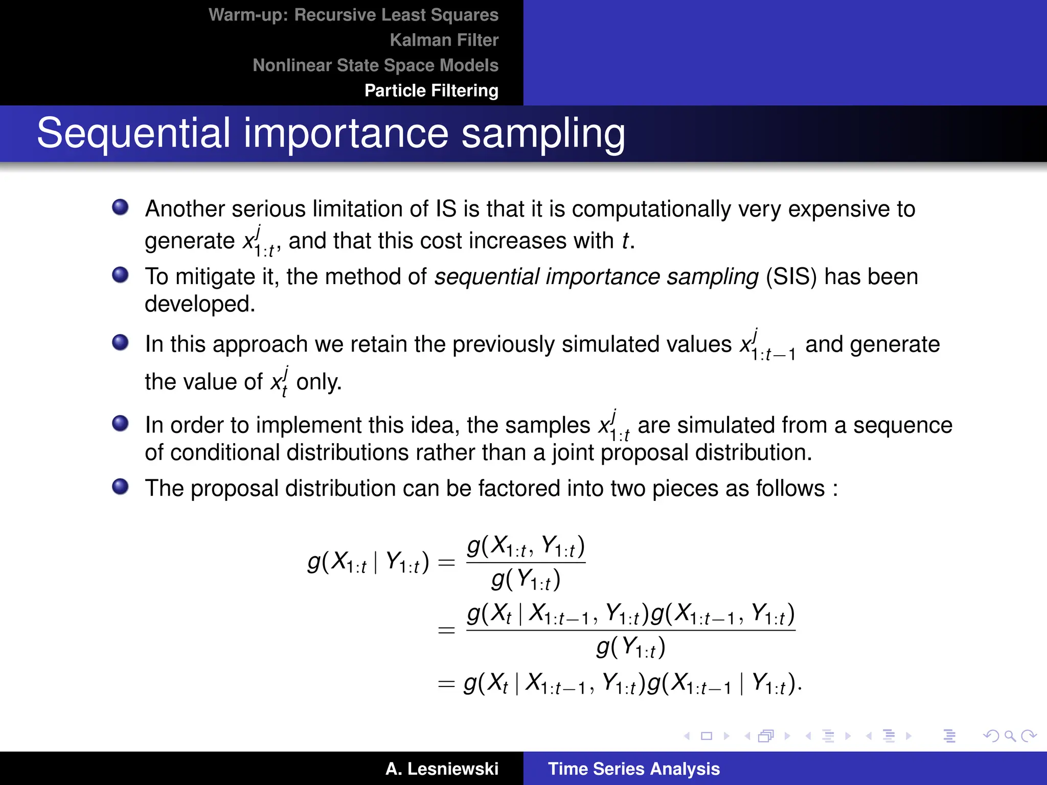
Another serious limitation of IS is that it is computationally very expensive to
generate x
j
1:t , and that this cost increases with t.
To mitigate it, the method of sequential importance sampling (SIS) has been
developed.
In this approach we retain the previously simulated values x
j
1:t−1 and generate
the value of x
j
t only.
In order to implement this idea, the samples x
j
1:t are simulated from a sequence
of conditional distributions rather than a joint proposal distribution.
The proposal distribution can be factored into two pieces as follows :
g(X1:t | Y1:t ) =
g(X1:t , Y1:t )
g(Y1:t )
=
g(Xt | X1:t−1, Y1:t )g(X1:t−1, Y1:t )
g(Y1:t )
= g(Xt | X1:t−1, Y1:t )g(X1:t−1 | Y1:t ).
A. Lesniewski Time Series Analysis
54.
Warm-up: Recursive LeastSquares
Kalman Filter
Nonlinear State Space Models
Particle Filtering
Sequential importance sampling
Once the sample of X1:t−1 has been generated from g(X1:t−1 | Y1:t−1), its value
is independent of the observation Yt , and so g(X1:t−1 | Y1:t ) = g(X1:t−1 | Y1:t−1).
We can thus write the result of the calculation above as the following recursion:
g(X1:t | Y1:t ) = g(Xt | X1:t−1, Y1:t )g(X1:t−1 | Y1:t−1). (65)
The second factor on the RHS of this equation, g(X1:t−1 | Y1:t−1), is the proposal
distribution built out of the paths that have already been generated in the
previous steps.
A new set of samples x1
t , . . . , xN
t is drawn from the first factor g(Xt | X1:t−1, Y1:t ).
We then append the newly simulated values x1
t , . . . , xN
t to the simulated paths
x1
1:t−1, . . . , xN
1:t−1 of length t − 1.
We thus obtain simulated paths x1
1:t , . . . , xN
1:t of length t.
A. Lesniewski Time Series Analysis
55.
Warm-up: Recursive LeastSquares
Kalman Filter
Nonlinear State Space Models
Particle Filtering
Sequential importance sampling
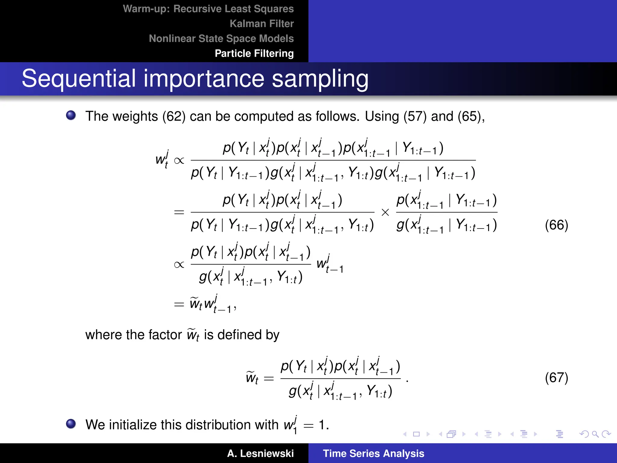
The weights (62) can be computed as follows. Using (57) and (65),
w
j
t ∝
p(Yt | x
j
t )p(x
j
t | x
j
t−1)p(x
j
1:t−1 | Y1:t−1)
p(Yt | Y1:t−1)g(x
j
t | x
j
1:t−1, Y1:t )g(x
j
1:t−1 | Y1:t−1)
=
p(Yt | x
j
t )p(x
j
t | x
j
t−1)
p(Yt | Y1:t−1)g(x
j
t | x
j
1:t−1, Y1:t )
×
p(x
j
1:t−1 | Y1:t−1)
g(x
j
1:t−1 | Y1:t−1)
∝
p(Yt | x
j
t )p(x
j
t | x
j
t−1)
g(x
j
t | x
j
1:t−1, Y1:t )
w
j
t−1
= e
wt w
j
t−1,
(66)
where the factor e
wt is defined by
e
wt =
p(Yt | x
j
t )p(x
j
t | x
j
t−1)
g(x
j
t | x
j
1:t−1, Y1:t )
. (67)
We initialize this distribution with w
j
1 = 1.
A. Lesniewski Time Series Analysis
56.
Warm-up: Recursive LeastSquares
Kalman Filter
Nonlinear State Space Models
Particle Filtering
Sequential importance sampling
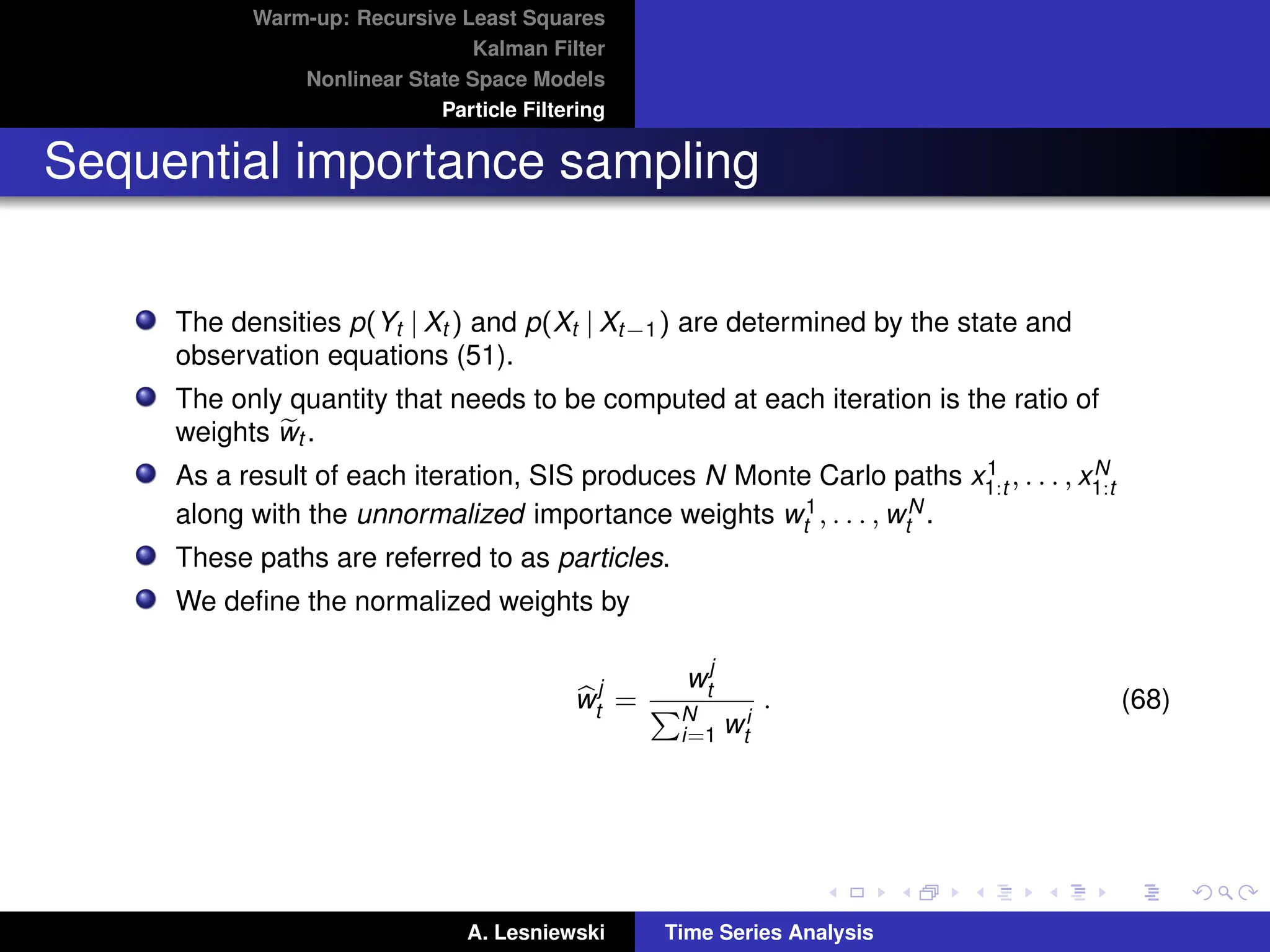
The densities p(Yt | Xt ) and p(Xt | Xt−1) are determined by the state and
observation equations (51).
The only quantity that needs to be computed at each iteration is the ratio of
weights e
wt .
As a result of each iteration, SIS produces N Monte Carlo paths x1
1:t , . . . , xN
1:t
along with the unnormalized importance weights w1
t , . . . , wN
t .
These paths are referred to as particles.
We define the normalized weights by
b
w
j
t =
w
j
t
PN
i=1 wi
t
. (68)
A. Lesniewski Time Series Analysis
57.
Warm-up: Recursive LeastSquares
Kalman Filter
Nonlinear State Space Models
Particle Filtering
Sequential importance sampling
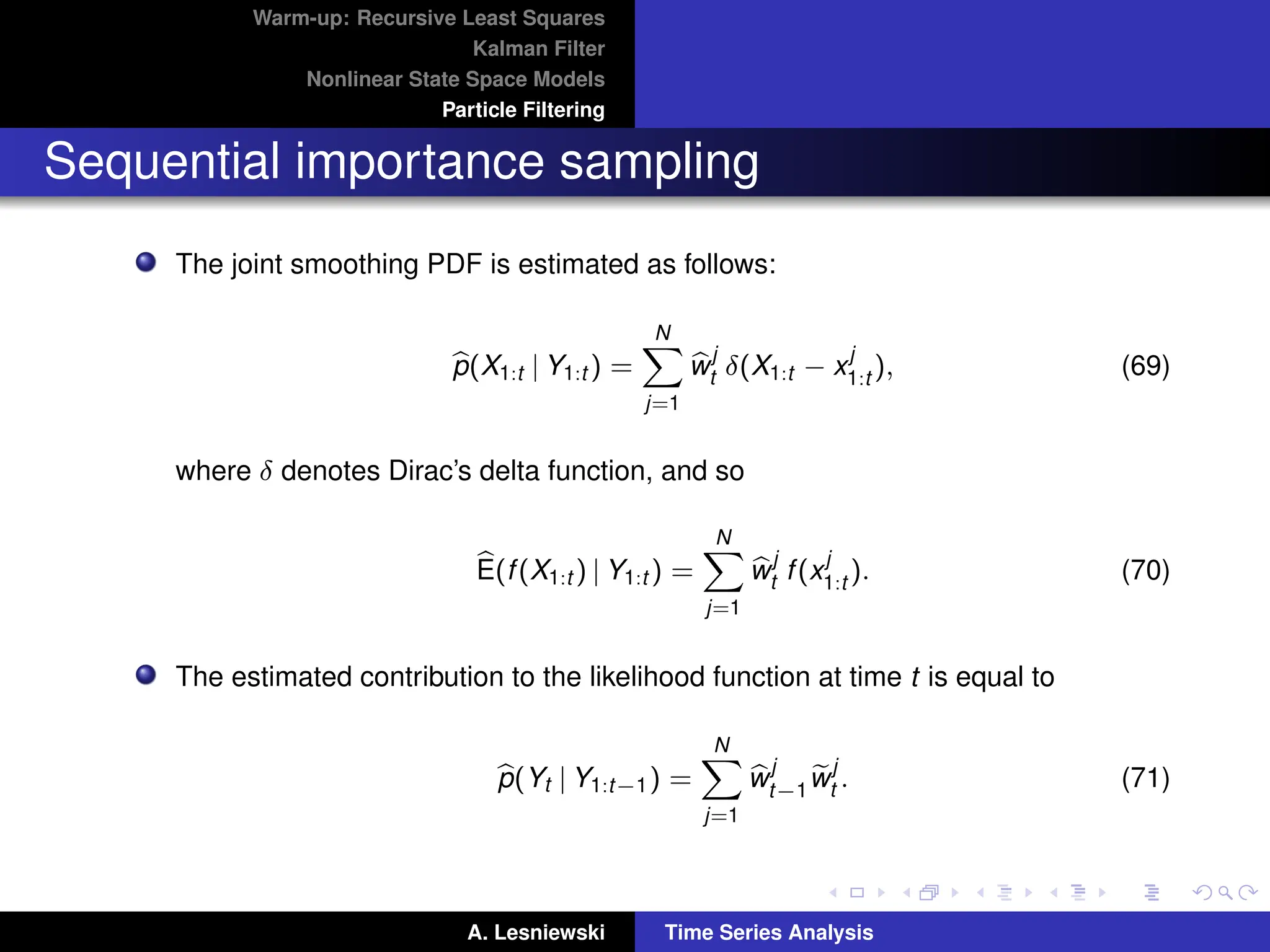
The joint smoothing PDF is estimated as follows:
b
p(X1:t | Y1:t ) =
N
X
j=1
b
w
j
t δ(X1:t − x
j
1:t ), (69)
where δ denotes Dirac’s delta function, and so
b
E(f(X1:t ) | Y1:t ) =
N
X
j=1
b
w
j
t f(x
j
1:t ). (70)
The estimated contribution to the likelihood function at time t is equal to
b
p(Yt | Y1:t−1) =
N
X
j=1
b
w
j
t−1
e
w
j
t . (71)
A. Lesniewski Time Series Analysis
58.
Warm-up: Recursive LeastSquares
Kalman Filter
Nonlinear State Space Models
Particle Filtering
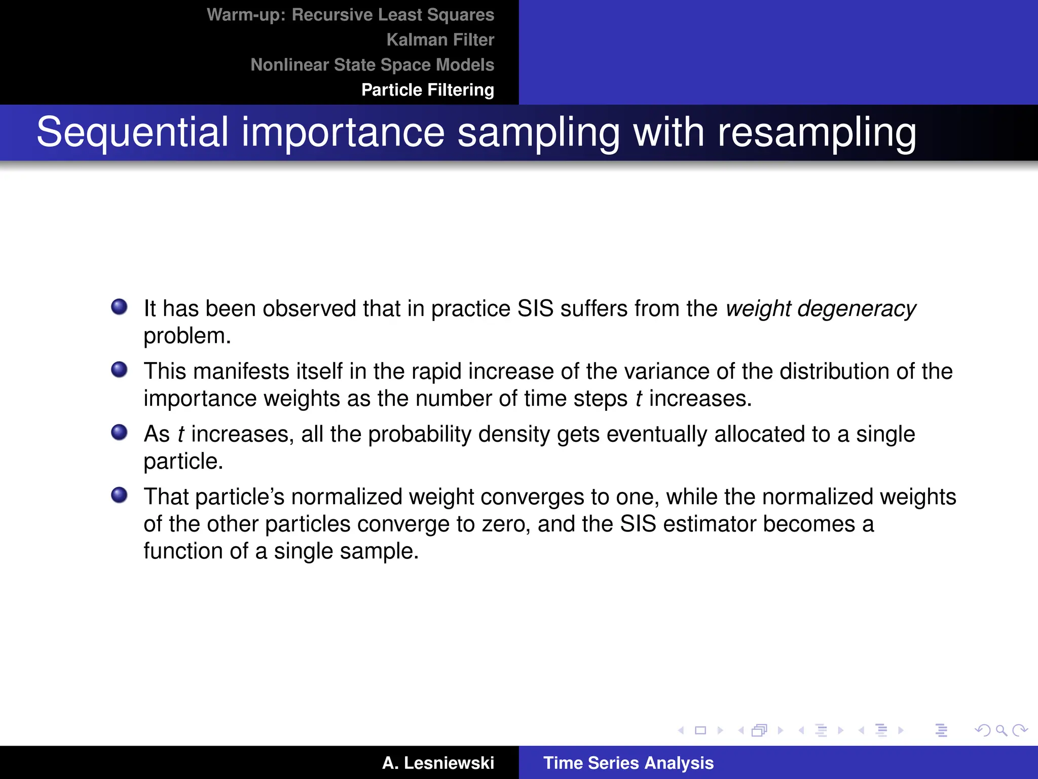
Sequential importance sampling with resampling
It has been observed that in practice SIS suffers from the weight degeneracy
problem.
This manifests itself in the rapid increase of the variance of the distribution of the
importance weights as the number of time steps t increases.
As t increases, all the probability density gets eventually allocated to a single
particle.
That particle’s normalized weight converges to one, while the normalized weights
of the other particles converge to zero, and the SIS estimator becomes a
function of a single sample.
A. Lesniewski Time Series Analysis
59.
Warm-up: Recursive LeastSquares
Kalman Filter
Nonlinear State Space Models
Particle Filtering
Sequential importance sampling with resampling
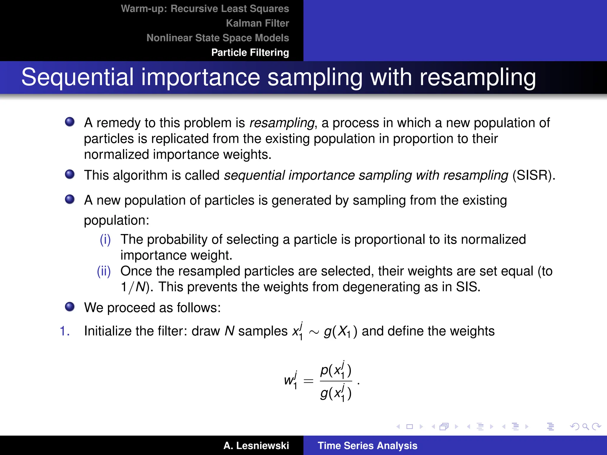
A remedy to this problem is resampling, a process in which a new population of
particles is replicated from the existing population in proportion to their
normalized importance weights.
This algorithm is called sequential importance sampling with resampling (SISR).
A new population of particles is generated by sampling from the existing
population:
(i) The probability of selecting a particle is proportional to its normalized
importance weight.
(ii) Once the resampled particles are selected, their weights are set equal (to
1/N). This prevents the weights from degenerating as in SIS.
We proceed as follows:
1. Initialize the filter: draw N samples x
j
1 ∼ g(X1) and define the weights
w
j
1 =
p(x
j
1)
g(x
j
1)
.
A. Lesniewski Time Series Analysis
60.
Warm-up: Recursive LeastSquares
Kalman Filter
Nonlinear State Space Models
Particle Filtering
Sequential importance sampling with resampling
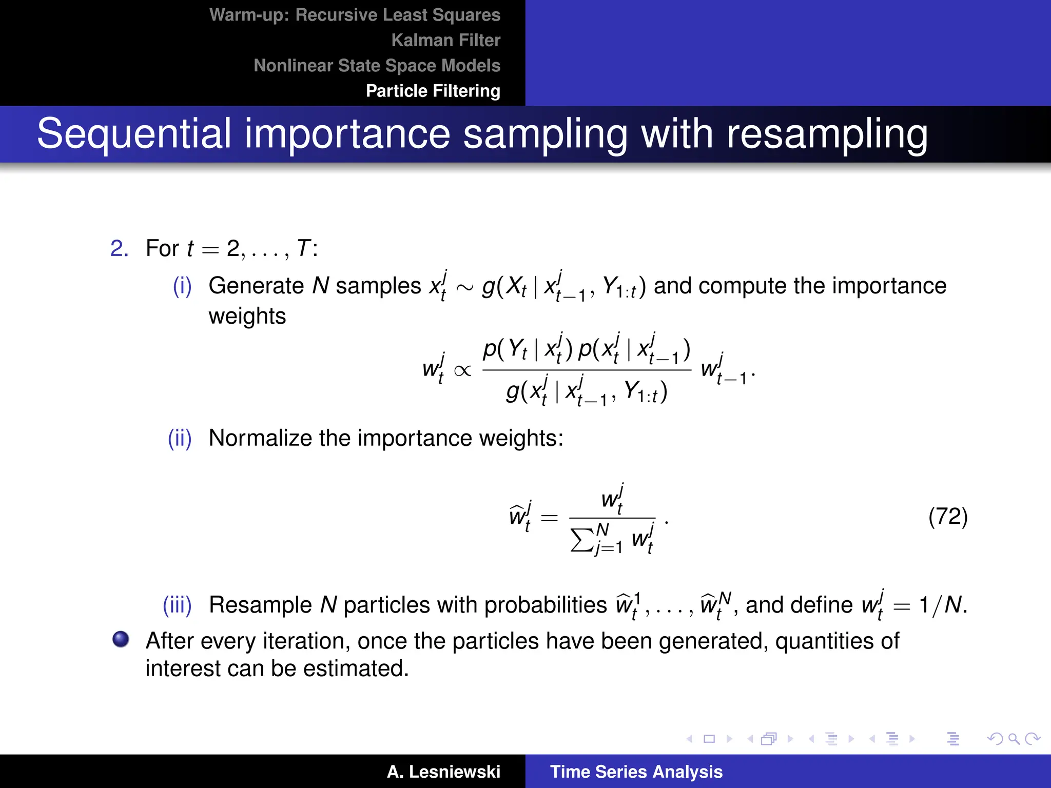
2. For t = 2, . . . , T:
(i) Generate N samples x
j
t ∼ g(Xt | x
j
t−1, Y1:t ) and compute the importance
weights
w
j
t ∝
p(Yt | x
j
t ) p(x
j
t | x
j
t−1)
g(x
j
t | x
j
t−1, Y1:t )
w
j
t−1.
(ii) Normalize the importance weights:
b
w
j
t =
w
j
t
PN
j=1 w
j
t
. (72)
(iii) Resample N particles with probabilities b
w1
t , . . . , b
wN
t , and define w
j
t = 1/N.
After every iteration, once the particles have been generated, quantities of
interest can be estimated.
A. Lesniewski Time Series Analysis
61.
Warm-up: Recursive LeastSquares
Kalman Filter
Nonlinear State Space Models
Particle Filtering
Sequential importance sampling with resampling
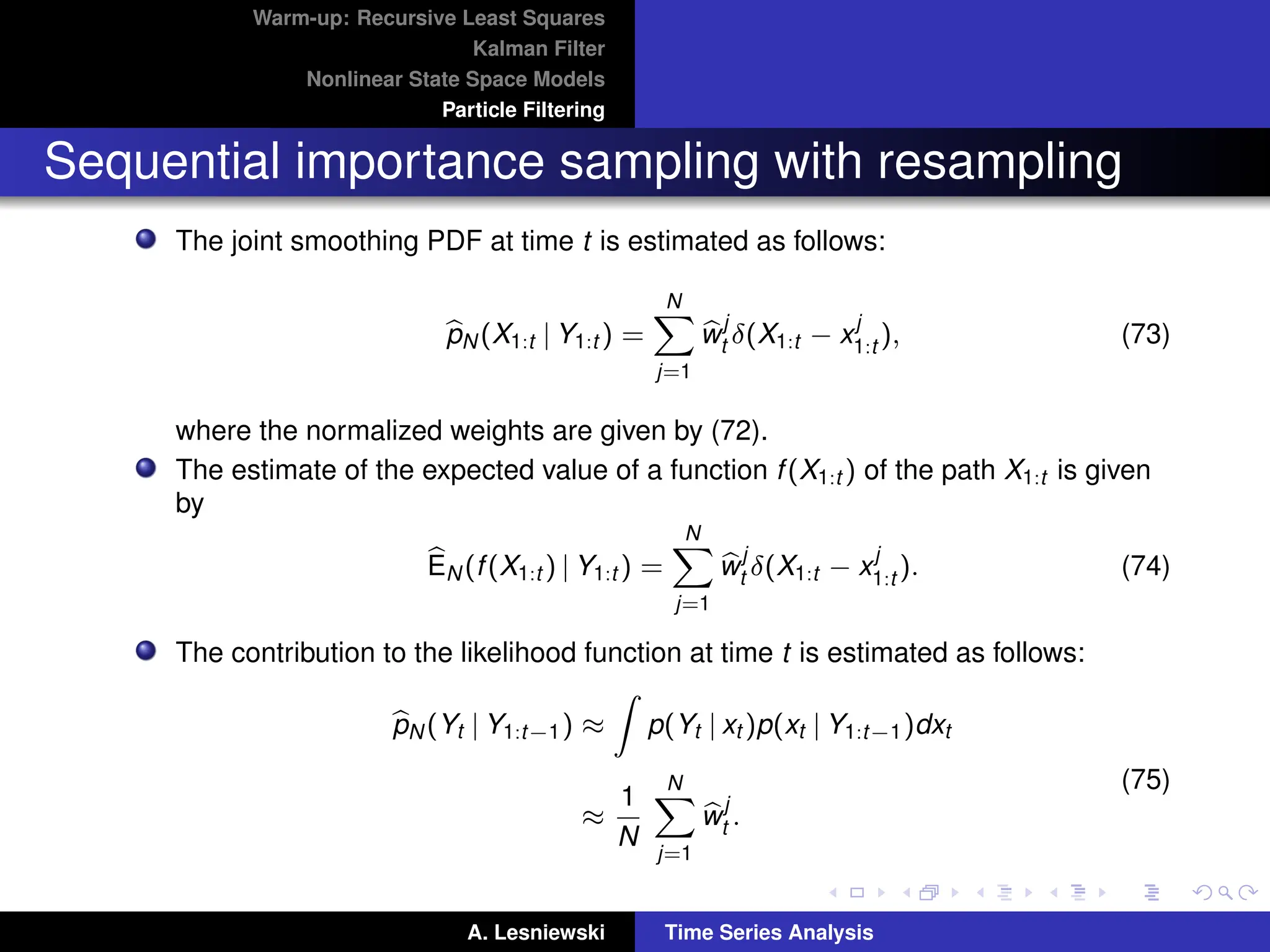
The joint smoothing PDF at time t is estimated as follows:
b
pN (X1:t | Y1:t ) =
N
X
j=1
b
w
j
t δ(X1:t − x
j
1:t ), (73)
where the normalized weights are given by (72).
The estimate of the expected value of a function f(X1:t ) of the path X1:t is given
by
b
EN (f(X1:t ) | Y1:t ) =
N
X
j=1
b
w
j
t δ(X1:t − x
j
1:t ). (74)
The contribution to the likelihood function at time t is estimated as follows:
b
pN (Yt | Y1:t−1) ≈
Z
p(Yt | xt )p(xt | Y1:t−1)dxt
≈
1
N
N
X
j=1
b
w
j
t .
(75)
A. Lesniewski Time Series Analysis
62.
Warm-up: Recursive LeastSquares
Kalman Filter
Nonlinear State Space Models
Particle Filtering
Bootstrap filter
The efficacy of the algorithms presented above depends on the choice of the
proposal distribution.
The simplest choice of the proposal distribution is
g(Xt | Xt−1, Yt ) = p(Xt | Xt−1). (76)
This choice is called the prior kernel, and the corresponding particle filter is
called the bootstrap filter.
The bootsstrap filter resamples by setting the incremental weight ratios equal to
e
wt = p(Yt | Xt ).
The prior kernel is an example of a blind proposal: it does not use the current
observation Yt .
Despite this, the bootstrap filter performs well in a number of situations.
Another popular version is the auxiliary particle filter, see [1] and [2].
A. Lesniewski Time Series Analysis
63.
Warm-up: Recursive LeastSquares
Kalman Filter
Nonlinear State Space Models
Particle Filtering
References
[1] Creal, D.: A survey of sequential Monte Carlo methods for economics and
finance, Economic Reviews, textbf31, 245 - 296 (2012).
[2] Durbin, J., and Koopman, S. J.: Time Series Analysis by State Space
Methods, Oxford University Press (2012).
A. Lesniewski Time Series Analysis
![Warm-up: Recursive Least Squares
Kalman Filter
Nonlinear State Space Models
Particle Filtering
State space models
A state space model (SSM) is a time series model in which the time series Yt is
interpreted as the result of a noisy observation of a stochastic process Xt .
The values of the variables Xt and Yt can be continuous (scalar or vector) or
discrete.
Graphically, an SSM is represented as follows:
X1 → X2 → . . . → Xt → . . . state process
y
y
y
y · · ·
Y1 Y2 . . . Yt . . . observation process
(8)
SSMs belong to the realm of Bayesian inference, and they have been
successfully applied in many fields to solve a broad range of problems.
Our discussion of SSMs follows largely [2].
A. Lesniewski Time Series Analysis](https://image.slidesharecdn.com/timeseriesanalysis-250411160716-01b0a04e/75/Time-series-Analysis-State-space-models-and-Kalman-ltering-10-2048.jpg)
![Warm-up: Recursive Least Squares
Kalman Filter
Nonlinear State Space Models
Particle Filtering
State smoothing
An analysis, similar to the derivation of the Kalman filter leads to the following
result (see [2]) for the derivation).
The smoothing process consists of two phases:
(i) forward sweep of the Kalman filter (28) for t = 1, . . . , T,
(ii) backward recursion
Rt−1 = HT
F−1
t vt + LT
t rt ,
Nt−1 = HT
F−1
t H + LT
t Nt Lt ,
b
Xt = µt + Pt Rt−1,
Vt = Pt − Pt Nt−1Pt ,
(33)
where Lt = G(I − Kt H), for t = T, T − 1, . . ., with the terminal condition
RT = 0 and NT = 0.
This version of the smoothing algorithm is somewhat unintuitive but
computationally efficient.
A. Lesniewski Time Series Analysis](https://image.slidesharecdn.com/timeseriesanalysis-250411160716-01b0a04e/75/Time-series-Analysis-State-space-models-and-Kalman-ltering-29-2048.jpg)
![Warm-up: Recursive Least Squares
Kalman Filter
Nonlinear State Space Models
Particle Filtering
MLE estimation of the parameters
For each t, the value of the log likelihood function is calculated by running the
Kalman filter.
Searching for the minimum of this log likelihood function using an efficient
algorithm such as BFGS, we find estimates of θ.
In the case of unknown µ1 and P1, one can use the diffuse log likelihood
method, which is discussed in detail in [2].
Alternatively, one can regard µ1 and P1 hyperparameters of the model.
A. Lesniewski Time Series Analysis](https://image.slidesharecdn.com/timeseriesanalysis-250411160716-01b0a04e/75/Time-series-Analysis-State-space-models-and-Kalman-ltering-35-2048.jpg)
![Warm-up: Recursive Least Squares
Kalman Filter
Nonlinear State Space Models
Particle Filtering
Nonlinear state space models
The recursion relations defining the Kalman filter can be extended to the case of
more general state space models.
Some of these extensions are straightforward (such as adding constant terms to
the right hand sides of the state and observation equations in (10)), others are
fundamentally more complicated.
In the remainder of this lecture we summarize these extensions following [2].
A. Lesniewski Time Series Analysis](https://image.slidesharecdn.com/timeseriesanalysis-250411160716-01b0a04e/75/Time-series-Analysis-State-space-models-and-Kalman-ltering-36-2048.jpg)
![Warm-up: Recursive Least Squares
Kalman Filter
Nonlinear State Space Models
Particle Filtering
Extended Kalman filter
The EKF works well if the functions G and H are weakly nonlinear, for strongly
nonlinear models its performance may be poor.
Other extensions of the Kalman filter have been developed, including the
unscented Kalman filter (UKF).
It is based on a different principle than the EKF: rather than approximating G and
H by linear expressions, one matches approximately the first and second
moments of a nonlinear function of a Gaussian random variable, see [2] for
details.
Another approach to inference in nonlinear SSMs is via Monte Carlo (MC)
techniques particle filters, a.k.a. sequential Monte Carlo.
A. Lesniewski Time Series Analysis](https://image.slidesharecdn.com/timeseriesanalysis-250411160716-01b0a04e/75/Time-series-Analysis-State-space-models-and-Kalman-ltering-43-2048.jpg)
![Warm-up: Recursive Least Squares
Kalman Filter
Nonlinear State Space Models
Particle Filtering
Bootstrap filter
The efficacy of the algorithms presented above depends on the choice of the
proposal distribution.
The simplest choice of the proposal distribution is
g(Xt | Xt−1, Yt ) = p(Xt | Xt−1). (76)
This choice is called the prior kernel, and the corresponding particle filter is
called the bootstrap filter.
The bootsstrap filter resamples by setting the incremental weight ratios equal to
e
wt = p(Yt | Xt ).
The prior kernel is an example of a blind proposal: it does not use the current
observation Yt .
Despite this, the bootstrap filter performs well in a number of situations.
Another popular version is the auxiliary particle filter, see [1] and [2].
A. Lesniewski Time Series Analysis](https://image.slidesharecdn.com/timeseriesanalysis-250411160716-01b0a04e/75/Time-series-Analysis-State-space-models-and-Kalman-ltering-62-2048.jpg)
![Warm-up: Recursive Least Squares
Kalman Filter
Nonlinear State Space Models
Particle Filtering
References
[1] Creal, D.: A survey of sequential Monte Carlo methods for economics and
finance, Economic Reviews, textbf31, 245 - 296 (2012).
[2] Durbin, J., and Koopman, S. J.: Time Series Analysis by State Space
Methods, Oxford University Press (2012).
A. Lesniewski Time Series Analysis](https://image.slidesharecdn.com/timeseriesanalysis-250411160716-01b0a04e/75/Time-series-Analysis-State-space-models-and-Kalman-ltering-63-2048.jpg)