This document summarizes the design and development of a laser sensor interface and tire DOT code scanning software. A laser sensor was selected to scan tire DOT codes due to its ability to create distance profiles of tire surfaces. A communication interface was built using a microcontroller, RS485 transceiver, and USB-to-serial converter to connect the laser sensor to a PC. Software was developed in C++ to control the sensor and acquire DOT code scans, and image processing techniques were explored in MATLAB and OpenCV to preprocess scan data. The laser sensor interface and scanning software provide an effective solution for reading important tire information like production dates from their DOT codes.


![Chapter 1
Introduction
This thesis report documents general information about vehicle tire codes, specifically tire
DOT code and its importance. Then different approaches for DOT code scanning are
analyzed and one of them is chosen. In the rest of this report, the selected approach is
documented, a communication interface is designed and built, a C++ software is developed
for data acquisition and at the end, some image pre-processing methods are performed.
1.1 General Tire Codes
In general, there are three unique codes embossed or engraved on the tire sidewalls.
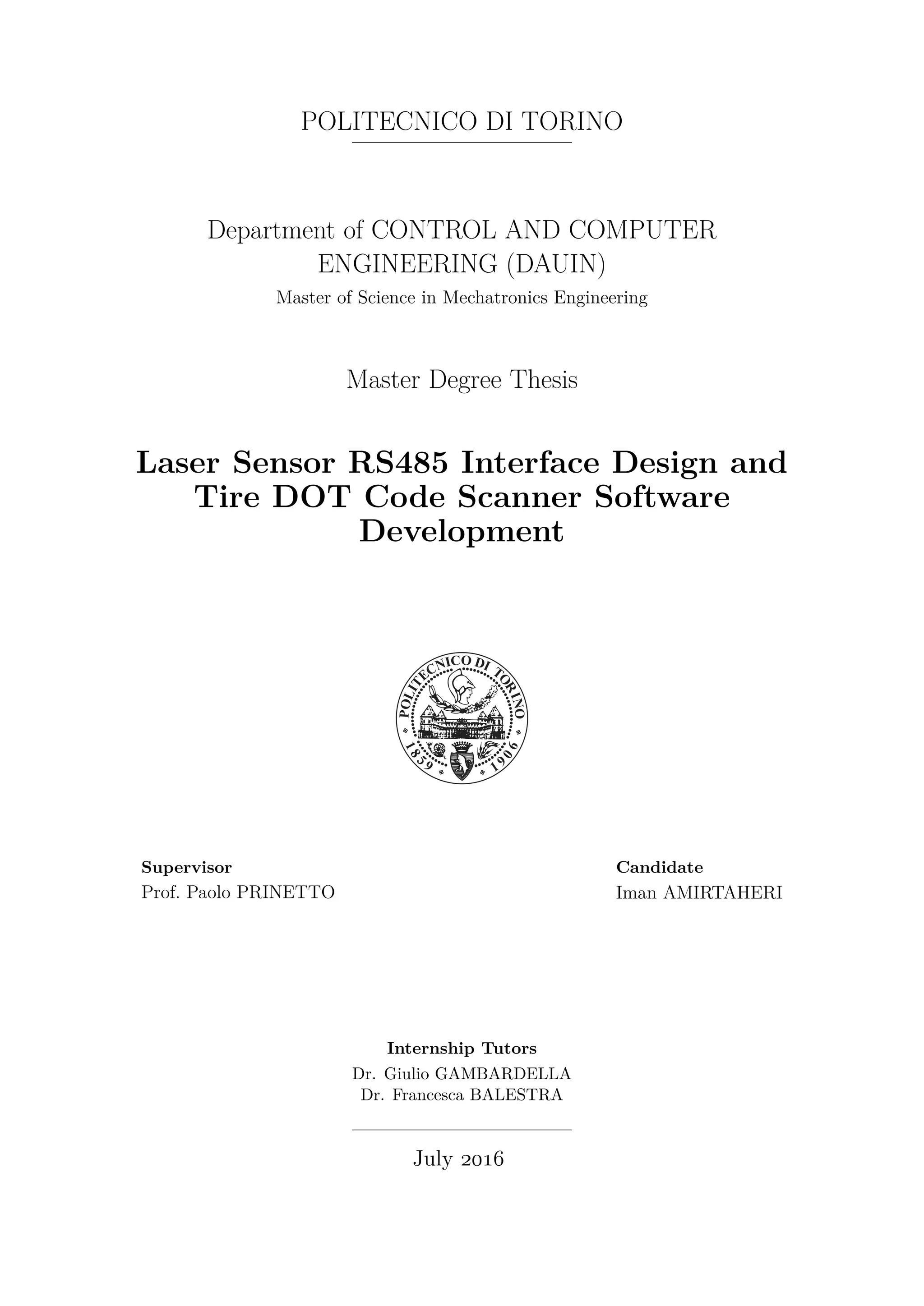
1.1.1 Tire Specification Code
This code contains information about tire type,tire width, aspect ratio between its height
and width,construction type, wheel diameter, load index and speed rating. Figure 1.1
shows an example of this code on tire sidewall. Note that this code in a real tire is colored
black but in this image for better legibility it is highlighted with white color. [1]
Figure 1.1. Tire Specification Code Sample: This code contains tire technical information.
1](https://image.slidesharecdn.com/a14ad75b-9842-4ff4-9b4c-90a45f40d9dc-160902161530/85/Thesis-Report-9-320.jpg)
![Iman AMIRTAHERI: Design RS485 Interface & DOT Code Scanner Software
1.1.2 Department of Transportation (DOT) Safety Code
Federal laws have obliged tire producer companies to determine the safety related infor-
mation of their tires on its sidewall. This code is named department of transportation
safety code and from now on it is referred to as DOT code. Figure 1.2 shows a sample of
this code.[1]
Figure 1.2. DOT Code Sample: All safety information is gathered inside this universal code.
DOT codes may consist of 8 upto 13 characters. Depending on the coding that manufac-
turer uses, the embedded information varies but in any case some important data has to
be documented. Some of these information fields are gathered in table 1.1.
Table 1.1. Tire DOT code information content
Characters
Index
Example
Characters
Definition
1-3 DOT DOT code identifier
4-5 B9 Tire’s Manufacturer and plant code
6-7 YR Tire size
8-11 UJNX Optional characters usually to determine brand and
other characteristics
12-13 50 Week of the year the tire was produced
14-15 08 Year the tire was produced (starts from year 2000)
1.1.3 Uniform Tire Quality Grading (UTQG) Code
This code was proposed by the national highway traffic safety administration to grade
tires based on their threadwear, traction and temperature. Figure 1.3 depicts a sample of
2](https://image.slidesharecdn.com/a14ad75b-9842-4ff4-9b4c-90a45f40d9dc-160902161530/85/Thesis-Report-10-320.jpg)
![1 – Introduction
this code.[1]
Figure 1.3. UTQG Code Sample: This code contains tire grades in three different subjects.
These grading subjects focus on quality figure of merits as described below.
• Threadwear
This grade determines how much this tire will last with comparison to the other
tires of this producer. Baseline grade is 100, and theoretically a tire with grade of
200 should last twice as long as tire with baseline grade.
• Traction
Traction grade is based on the tire ability to stop on a wet road. There is a standard
road which is used to perform this test on tires. Acceptable grades from high to low
are AA,A,B and C. Tires with traction grade of less than C are not qualified to be
used for road travels.
• Temperature
One of the most important items in tires world is the ability of tire to dissipate heat.
There is a standard controlled indoor test which benchmarks tires heat dissipation
and grade them starting from A for the best ones. Tires with the grade of D and
below are considered unacceptable.
1.2 Tire Replacement Symptoms
Car tires are not designed to last forever and the they have to be changed on a regular
basis. There are two important items on tire checklist which recommend the car owner to
replace tires when at least one of them is checked.
1.2.1 Tire Treads Depth
Tire treads are designed to maintain sufficient interaction between tire and road surface.
After a period of time, tires begin to wear out and lose their treads depth. Most of tire
3](https://image.slidesharecdn.com/a14ad75b-9842-4ff4-9b4c-90a45f40d9dc-160902161530/85/Thesis-Report-11-320.jpg)
![Iman AMIRTAHERI: Design RS485 Interface & DOT Code Scanner Software
producers recommend costumers to change tires as soon as the tire treads depth fall less
than 2/32-inch (1.6mm). Figure 1.4 shows corresponding life time for each level of tread’s
depth. [2]
Figure 1.4. Tire Tread Depth: Tire producers recommend to replace tires
with less than 10% life time.
From longtime ago tread depth measurement was performed by means of length measure-
ment devices such as calipers. Even many of auto repairmen use a small coin to measure
depth. Although this kind of approach is not wrong and use the same principle but it is
not accurate enough because it is necessary to measure and check precisely not only for a
single spot of tire but also for all of it’s surface. So the accurate procedure is very time
consuming for an auto repairman to follow.
Tire Profiles Italy Srl. company has designed two different solutions to measure tread’s
depth.
• Groove Glove Scanner
This handheld device is designed to measure tire depth and also identify car license
plate by means of laser triangulation and camera OCR respectively. Tire surface
is scanned by moving the device over it. Scanned data gets transferred to a cloud
server and required processes are performed inside there. Figure 1.5 shows a Groove
Glove Scanner device.[4]
• TreadSpec
TreadSpec also known as PRT Scanner is a device which requires a solid structure to
mount on the ground surface. This solution is usually used on the entry point of auto
service centers and allows the driver to drive over it. In many cases people pay service
centers a visit just to change oil or diagnose an error, with this scanner installed in
the entrance, service centers generate a full report about tire tread depth and its
alignment. Hence, this device can boost their sale effectively. Figure 1.6 shows two
4](https://image.slidesharecdn.com/a14ad75b-9842-4ff4-9b4c-90a45f40d9dc-160902161530/85/Thesis-Report-12-320.jpg)
![1 – Introduction
Figure 1.5. Groove Glove Scanner: Handheld device to measure tire tread depth
and identify car’s license plate.
pictures of this device combined. [3]
Figure 1.6. TreadSpec (PRT Scanner): Tread depth scanner which has to be
installed on the ground.
1.2.2 Tire Expiry Date
Despite from level of tire thread depth, it is crucial to replace the tire on a regular basis.
Most of tire producers guarantee their product for five years from the week that it was
produced.[5] So another interesting area for auto service centers is to have a device like
Groove Glove Scanner which determines the tire age. As mentioned in 1.1 on page 2, the
DOT code printed on the tire sidewall has the valuable information which indicates the
production week and year.
5](https://image.slidesharecdn.com/a14ad75b-9842-4ff4-9b4c-90a45f40d9dc-160902161530/85/Thesis-Report-13-320.jpg)

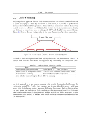
![Iman AMIRTAHERI: Design RS485 Interface & DOT Code Scanner Software
Figure 2.1. Fixed Illumination: Naive approach to illuminate tire surface and
capture DOT code.
This prototype masks the ambient light thanks to its method of usage which is touching
tire surface. Instead, it has many infrared diodes to illuminate the DOT code when it
captures the photo. Since these illumination lamps are turned on and off simultaneously
and the camera axis is perpendicular to tire surface, it is not possible to distinguish
characters since tire codes are embossed or raised on the body of tire and it is a black on
black pattern.
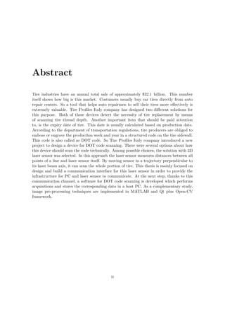
In order to overcome this problem variable illumination technique (structured lighting)
has proposed[14]. Since the DOT code is only detectable due to its altitude difference,
variable illumination technique can eliminate background and just maintain the raised
code. This technique turns on then lights one by one and captures a photo each time,
because of altitude difference in tire surface each time the resulting shadow will be different.
Then a sophisticated algorithm gathers all of these photos and combine them together
based on the shadows. At the end, the obtained final photo shows only DOT code and
eliminates its background. Figure 2.2 shows a simplified version of this approach. Usually
there are at least 8 lights to illuminate tire surface and they are placed on a circular base.
This method is also called as structured lighting.
Figure 2.2. Variable Illumination: Camera captures every time that illumination changes.
8](https://image.slidesharecdn.com/a14ad75b-9842-4ff4-9b4c-90a45f40d9dc-160902161530/85/Thesis-Report-16-320.jpg)

![Chapter 3
Laser Sensor
So far, the desired design approach is selected. In this chapter, the laser sensor is in-
troduced, its features are documented and an appropriate communication interface is de-
signed. Sensor selection is another decision which was imposed by the Tire Profiles Italy
company. For administrative and economical reasons, this sensor was already selected and
purchased for this project.
3.1 Functional Criterion
The selected sensor is produced by Baumer company and its from MESAX multi -distance-
measuring sensors family. It measures distances and heights of objects and was specially
developed for easy handling. Also it makes use of a red beam to help sensor alignment.
Table 3.1 denotes functioning criteria for the sensor OM70B-15LB-11125351.[6]
Table 3.1. Laser Sensor Functional Criterion
Function Valid Criteria
Start of measuring range 100mm
End of measuring range 150mm
Measuring field width left 36mm
Measuring field width right 36mm
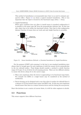
3.2 Installation
According to sensor’s datasheet provided by Baumer company [6], it can be installed in
two different methods.
• Standard Installation
In this configuration sensor is mounted at a right angle with respect to the surface.
11](https://image.slidesharecdn.com/a14ad75b-9842-4ff4-9b4c-90a45f40d9dc-160902161530/85/Thesis-Report-19-320.jpg)
![3 – Laser Sensor
not at the same time. Full duplex mode defines a similar connection but with capability
to send and receive simultaneously. This protocol requires two wires for half duplex mode
and four wires for full duplex transmission. According to Baumer sensors datasheet, fig-
ure 3.5 shows required configuration in order to connect upto fifteen sensors to a master.[7]
Figure 3.5. RS485 Connection Diagram: This protocol can connect 15 sensors to a master.
The most important features of this topology are listed in this way.
• Master is the only member of this configuration which can initiate a request. Sensors
are slaves, so they do no transmit anything unless master asks for it.
• This configuration can support a baud rate of 115kbit/s at max.
• Maximum possible length of cable is 10m.
• RS485 cables must be shielded.
• There are two failsafe resistors called RB to define the resistance level when no
transmitter is active.
Since there is only one sensor to work with, first topology is selected for communication.
This sensor came with a default shielded cable. Figure 3.6 denotes corresponding pin
diagram for this cable.
The suggested voltage supply for this sensor is 24v. Also it is recommended to connect
15](https://image.slidesharecdn.com/a14ad75b-9842-4ff4-9b4c-90a45f40d9dc-160902161530/85/Thesis-Report-23-320.jpg)

![3 – Laser Sensor
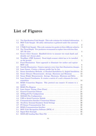
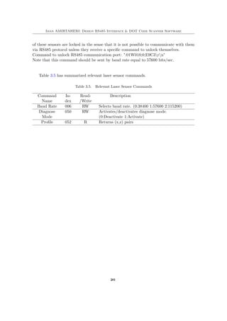
3.5 Time Flows
RS485 commands must be sent through a certain structure so the sensor can interpret
and response appropriately. Before listing the possible commands, it is better to dedicate
a few sentences about communication speed. It is preferred to describe this matter in
current section rather than previous one because it is actually possible to modify the
communication speed via commands.
This laser sensor can work with three different baud rates.[7]
1. 38400 bits/s
2. 57600 bits/s
3. 115200 bits/s
The default configuration for baud rate is 57600 bits/sec. It means that every time that
sensor is powered on, it automatically interprets incoming requests with baud rate of
57600. Also it is possible to change this value with corresponding command and save it
to configuration flash.
Since the application goal is to make acquisition with the highest possible rate, the sensor
timing to response the request is very crucial. Figure 3.7 denotes various timing variables
and table 3.3 determines their values.
Figure 3.7. Laser Sensor Timing (Time Flows)
Since the application must use the sensor in diagnose mode, the maximum time re-
quired by sensor to process the request and prepare appropriate response can be derived
as follows.
(tsmax)noerror = tanswerdiagmode = 200ms
(tsmax)error = tbreak = 500ms
To make a rough calculation about order of acquisition rate, lets assume that field of
view attribute is set to 4cm. In other words, laser sensor is scanning only line with width
of 4cm per each acquisition iteration. According to table 3.2 on page 14, laser sensor
returns a pair of x and z elements for each 0.5mm of field of view.
Total number of pairs = 4cm
0.5mm = 80
17](https://image.slidesharecdn.com/a14ad75b-9842-4ff4-9b4c-90a45f40d9dc-160902161530/85/Thesis-Report-25-320.jpg)

![3 – Laser Sensor
this laser sensor is not suitable for the real action, but since this sensor has been already
purchased, the prototype designing was based on this sensor.
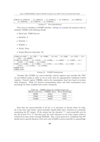
3.6 Commands
In previous sections, all important features of laser sensor and its communication rules
were analyzed. In this section, relevant commands are listed and described. Every single
command has to have a predefined structure in order to be decode-able for laser sensor.[7]
Command structure consists of following ordered items:
• Start identifier: A simple colon character ":" is used to acknowledge beginning of a
command.
• Device address: Two digits have the responsibility to determine target device ID.
All sensors have address equal to 01 at power on instant. In order to have more than
one sensor in a network, sensors ID must be configured one by one such a way that
there will be no conflict among them.
• Payload: This part of command can have different number of characters depending
on the command format. Payload itself consists of:
– Type: It can be "W" or "R" to determine the command is to write or read a
content respectively.
– Index: This item has three characters and form a number. Every single com-
mand which is supported by laser sensor has an ID called index. To perform a
desired operation, command must specify the corresponding index. Note that
it is possible for a single index to support both write and read operations.
– Separator: A semicolon character ";" is used before and after of each payload
element to clarify elements from each other.
– Payload element: If the desired command requires a payload element (data) to
perform operation, desired data should be placed in payload element. Note that,
it is possible to have many payload elements separated by semicolon separator.
• CHECKSUM: This code is generated by CRC-16 algorithm in order to avoid cor-
rupted command execution. CHECKSUM code is generated by the master and will
be controlled by slave upon message receipt. This code can be overridden by using
"****" code instead.
• Termination characters: A combination of carriage return "r" and line feed "n"
characters is used to determine the command’s end. The same characters are used
to represent a new line in Microsoft Windows operating systems.
Most of laser sensors in the category of "MESAX multi-distance measuring" have a
built in display and user input. This specific sensor does not have this feature because
there is no intention to interact with the laser sensor directly. With this introduction, all
19](https://image.slidesharecdn.com/a14ad75b-9842-4ff4-9b4c-90a45f40d9dc-160902161530/85/Thesis-Report-27-320.jpg)
![Iman AMIRTAHERI: Design RS485 Interface & DOT Code Scanner Software
points to consider:
• Output levels of micro-controller must use TTL logic, because RS485 uses TTL logic
for each wire otherwise there is a need for level shifter.
• It must have dedicated ports for UART/USART communication.
• It is recommended to have SPI port for further wireless module or gyroscope addition.
• In order to work with the highest possible baud rate, micro-controller has to be able
to work with 11.0592MHz clock. This clock assures that UART/USART communi-
cation error will be less than 0.0%.
According to these requirements, ATMega16 micro-controller was the selected choice
among AVR micro-controllers. In the rest of this chapter, technical relevant characteristics
of this device are documented.[9]
4.1.1 General Overview
This little and cheap micro-controller has many features, here are the most important
ones.
• Operating Voltage: 2.7V - 5.5V
• Speed Grade: 0 - 8 MHz
• I/O and Packages
– 32 Programmable I/O Lines
– 40-pin DIP, 44-lead TQFP and 44-pad QFN/MLF
• Peripheral features
– Programmable Serial USART
– Master/Slave SPI Serial Interface
– Byte-Oriented Two-wire Serial Interface
– Four Timer/Counters
– Four PWM Channels
• 32*8 General Purpose Working Registers
• Non-volatile Memory Segments
– 16Kbytes of fIn-System Self-programmable Flash program memory
– 512 Bytes EEPROM
– 1 Kbyte Internal SRAM
The micro-controller used for this project was packaged in DIP format because in this way
it is much easier to use it on bread board.
22](https://image.slidesharecdn.com/a14ad75b-9842-4ff4-9b4c-90a45f40d9dc-160902161530/85/Thesis-Report-30-320.jpg)
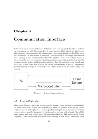
![4 – Communication Interface
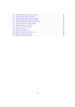
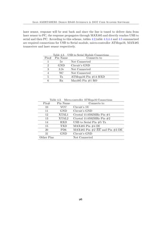
4.1.2 Pin Configurations
Figure 4.2 denotes pin configurations for ATMega16 micro-controller. Some of pins have
dual functions and they can be selected by software. For example pin #14 is the IO #0
of port D in normal condition. It can be configured to function as serial receiver also.
Figure 4.2. ATMega16 Pin Configurations
4.1.3 Universal Synchronous Asynchronous Receiver Transmitter (US-
ART)
In order to manage the RS485 connection between PC and the laser sensor, micro-
controller has to work with its USART block. According to the pin configurations on
figure 4.2, table 4.1 denotes all USART related pins.[9]
Table 4.1. USART Pins
Pin# Normal
Function
USART
Function
Description
14 PD0 RXD USART receiver input.
15 PD1 TXD USART transmitter output.
11 GND GND Should be connected to the PC and laser sensor
grounds to share the same voltage levels.
23](https://image.slidesharecdn.com/a14ad75b-9842-4ff4-9b4c-90a45f40d9dc-160902161530/85/Thesis-Report-31-320.jpg)
![Iman AMIRTAHERI: Design RS485 Interface & DOT Code Scanner Software
4.2 RS485 Transceiver
Using micro-controller as the medium does not mean that USART output can be con-
nected to RS485 wires. As previously mentioned RS485 can use two or four wires for
communication in half duplex or full duplex mode respectively. This laser sensor supports
only the half duplex mode, That’s why its designers have considered only two wires for
communication in RS485 shielded cable. In order to plug USART output to RS485 con-
nection a transceiver is required. One of the most common solutions for this problem is
MAX485 integrated circuit.[10]
Figure 4.3 shows MAX485 transceiver pin configuration. As it is possible to observe in
the figure, this IC is composed of two tri-state buffers. RE and DE has the responsibility
to control these buffers. RS485 uses two wires to transmit one bit in differential format.
For example in order to represent a "0" logic A has "0" value and B has "1" value. The dif-
ference between these two levels which for this case is -5V, determines that the sender has
sent "0". Its exactly vice versa when sender is transmitting "1". So two control signals, RE
and DE select that master is going to send a command or receive a response respectively.
During command sending DE is set to "1" and RE is set to "0". It is opposite when laser
sensor is transmitting response. DI connects to TXD of micro-controller and RO should
be connected to PC. More information will be provided during this chapter.
Figure 4.3. MAX485 Pin Configuration
4.3 USB to Serial Converter
A few years ago, it was very common for personal computers and laptops to have port
for serial connection. Nowadays it is completely rare to have this kind of port for normal
computers and there are only USB ports that can do the same thing. In order to send
and receive in a serial connection, operating system needs to open a COM port. USB to
Serial converters create a virtual COM port so PC can threat with it like a normal one.
At the other side there is a small circuit to convert USB data signals (D+ and D−) to Rx
and Tx signals. Figure 4.4 depicts a USB to Serial converter module. It has a USB port
24](https://image.slidesharecdn.com/a14ad75b-9842-4ff4-9b4c-90a45f40d9dc-160902161530/85/Thesis-Report-32-320.jpg)
![4 – Communication Interface
so a USB cable can connect it to PC. There are also five pins which three of them deliver
GND, 3.3V and 5V and the two remaining form the serial connection wires (Rx and Tx).
This is not a complicated module, most of USB to Serial converters make use of PL2303
chip for data conversions.[11]
Figure 4.4. USB to Serial Converter Module
4.4 Hardware Connections
So far, required elements have been introduced. In this section, connections between these
elements are described. Figure 4.5 depicts all required connections between previously
described elements.
Figure 4.5. Communication Interface Connection Scheme
In this scheme, PC which is the final device to send commands to laser sensor and
receive response from it, is connected to USB to Serial converter via a simple USB cable. So
in the PC, by installing appropriate driver, it is possible to open a COM port and transmit
serial data. Commands sent by PC are delivered to micro-controller. Micro-controller has
the responsibility to control RS485 connection. This control means that, if there is a
command to be delivered to laser sensor, micro-controller prepares the line by setting DE
to "1" and RE to "0". In this way line is ready to accept value from micro-controller. While
this situation exists, the command is sent to laser sensor. Micro-controller will change the
line situation immediately after sending is finished. In this way the command is sent and
line is ready to receive answer from laser sensor. After computation time required by
25](https://image.slidesharecdn.com/a14ad75b-9842-4ff4-9b4c-90a45f40d9dc-160902161530/85/Thesis-Report-33-320.jpg)

![Chapter 5
Acquisition Software
In previous chapter, a communication interface was designed and built to make PC-Sensor
communications possible. A sample command sent by means of TeraTerm terminal emula-
tor and corresponding responses received. In this chapter, the goal is to design a software
to automate this process. So the software should be able to initiate a connection to the
laser sensor, send requests, receive responses, display them in a graphical way and store
them in a file for further usage.
In order to have possibility to compile the program for different operating systems and
also for accessing to simpler features, Qt IDE has been used for software development.
Qt IDE is developed and supported by Nokia company. Nowadays many programmers
and developers use Qt for software development. Figure 5.1 depicts the first version of
acquisition program designed. During rest of this chapter different program sections will
be analyzed.[12]
Figure 5.1. DOT Code Recognition Software (DCR) v1
Qt IDE supports signals and slots methodology for objects communication. During
33](https://image.slidesharecdn.com/a14ad75b-9842-4ff4-9b4c-90a45f40d9dc-160902161530/85/Thesis-Report-41-320.jpg)
![Iman AMIRTAHERI: Design RS485 Interface & DOT Code Scanner Software
void DiagnoseMode ( bool Switch ) ;
30 void P r o f i l e ( int Xpos [ 3 0 0 ] , int Zpos [ 3 0 0 ] ) ;
void SensorTimedOut ( bool Switch ) ;
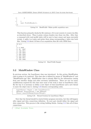
32 void ProfileReady () ;
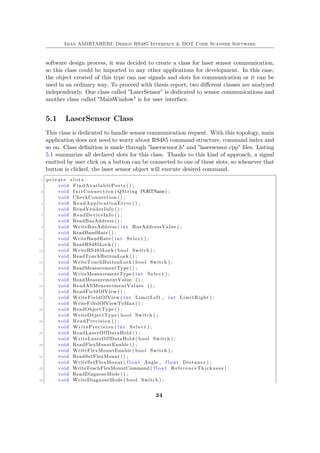
Listing 5.2. LaserSensor Class Signals
So with these slots and signals, all requests are sent through slots and all responses
are emitted via signals. Now lets go into the details and analyze the most important slots
functions.
• Laser Sensor Constructor:
This function is called whenever a new object of class LaserSensor is created. This
initializes serial communication and sets its baud rate to 115200 bits/sec. This serial
connection uses a Qt library called "QtSerial.h". After serial port initialization,
it initialize some other variables that will be covered later. Listing 5.3 denotes
LaserSensor constructor definition.
LaserSensor : : LaserSensor ()
2 {
qRegisterMetaType<QVector<QString> >(" QVector<QString>" ) ;
4 s e r i a l = new QSerialPort ( t h i s ) ;
s e r i a l −>setBaudRate ( QSerialPort : : Baud115200 ) ;
6 s e r i a l −>setDataBits ( QSerialPort : : Data8 ) ;
s e r i a l −>setParity ( QSerialPort : : EvenParity ) ;
8 s e r i a l −>setStopBits ( QSerialPort : : OneStop ) ;
s e r i a l −>setFlowControl ( QSerialPort : : NoFlowControl ) ;
10 DeviceAddress =1;
Yindex=0;
12 f i l e c r e a t e d=f a l s e ;
SampleNo=" 1 " ;
14 }
Listing 5.3. LaserSensor Constructor
The third line of code has the duty to register a meta type in order to provide
possibility to move an object of this class to a new thread. DeviceAddress variable
is always one since there is only one sensor in RS485 network. Yindex is the index
of scanned lines and it is set to zero at first. After each successful acquisition it will
be automatically incremented. filecreated flag is used to check if the profile text file
is created or not. In read profile mode, laser sensor class should store acquisition
data in a text file. SampleNo variable is defined to identify different tire samples. It
is just there for further result comparisons.
• FindAvailablePorts
This function scans for all COM ports, then removes those ones that are not available.
A COM port is not available when another program is using it and it is flagged as
busy. Then it emits a signal containing total number of available ports and their
names. Listing 5.4 denotes corresponding codes.
void LaserSensor : : FindAvailablePorts ()
36](https://image.slidesharecdn.com/a14ad75b-9842-4ff4-9b4c-90a45f40d9dc-160902161530/85/Thesis-Report-44-320.jpg)
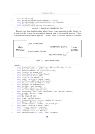
![5 – Acquisition Software
}
Listing 5.7. WriteDiagnoseMode: Activates diagnose mode.
Although this function is designed to just activate the diagnose mode, it also sets the
field of view range. In third line, laser sensor is asked to set its measuring range from
-20mm to 20mm with respect to the center of red beam. Then the same attribute
requested to read for verification. Finally at line 7, program sends diagnose mode
activation command and if the response is received, it emits a signal to MainWindow
which yields to a check in a checkbox.
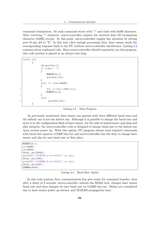
• ReadProfile
Finally, its time to analyze the main function that collects acquisition data. This
function creates two data files and store the same content into both of them. The
reason of creating two identical files is that, for image pre-processing part, it was
necessary to address a constant file name in MATLAB. In order to prevent from
overwriting the previously made acquisition, another file with date, time and also
sample number is created each time. According to listing 5.8, this function performs
a profile acquisition once and emits a ProfileReady signal when its done. This is the
duty of MainWindow to call this function in a loop to scan multiple lines.
void LaserSensor : : ReadProfile ()
2 {
i f ( ! f i l e c r e a t e d )
4 {
QDateTime currentdateandtime = QDateTime : : currentDateTime () ;
6 ProfileData . setFileName ( " ProfileData_Sample "+SampleNo+"_"+
currentdateandtime . toString ( " yyyy−MM−dd_hh−mm−ss " )+" . txt " ) ;
ProfileData . open ( QIODevice : : WriteOnly ) ;
8 ProfileData1 . setFileName ( " ProfileData . txt " ) ;
ProfileData1 . open ( QIODevice : : WriteOnly ) ;
10 ProfileStream . setDevice(&ProfileData ) ;
ProfileStream << "YtX t Z" <<endl <<endl ;
12 ProfileStream1 . setDevice(&ProfileData1 ) ;
ProfileStream1 << "YtX t Z" <<endl <<endl ;
14 f i l e c r e a t e d=true ;
}
16 SendCommand( "R052" ) ;
i f ( ReceiveResponse () )
18 {
QStringList XZMeasurements ;
20 XZMeasurements=Payloads [ 1 ] . s p l i t ( " " ) ;
int TotalMeasurements=XZMeasurements [ 0 ] . toInt () ;
22 XZMeasurements . removeFirst () ;
Yindex++;
24 f o r ( int i =0; i<TotalMeasurements /2; i++)
{
26 ProfileStream << Yindex <<" t " << XZMeasurements [2 ∗ i ] <<" t
" <<XZMeasurements [2 ∗ i +1] <<endl ;
ProfileStream1 << Yindex <<" t " << XZMeasurements [2 ∗ i ] <<"
t " <<XZMeasurements [2 ∗ i +1] <<endl ;
39](https://image.slidesharecdn.com/a14ad75b-9842-4ff4-9b4c-90a45f40d9dc-160902161530/85/Thesis-Report-47-320.jpg)

![Iman AMIRTAHERI: Design RS485 Interface & DOT Code Scanner Software
17 [ r , c ] = s i z e ( t r i ) ;
disp ( r )
19
h = t r i s u r f ( t r i , x , y , z ) ;
21 axis vis3d
axis o f f
23 l = l i g h t ( ’ Position ’ ,[ −50 −15 29 ] ) ;
set ( gca , ’ CameraPosition ’ ,[208 −50 7687]) ;
25 l i g h t i n g phong
shading interp
27 colorbar EastOutside
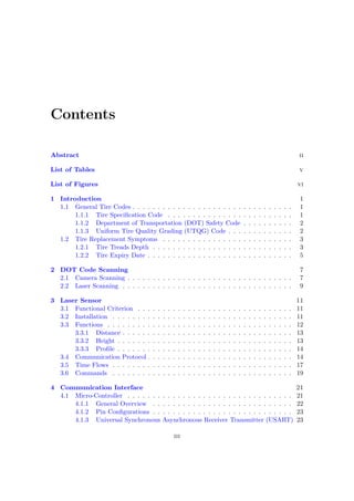
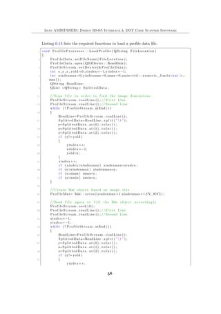
Listing 6.1. Data file loading
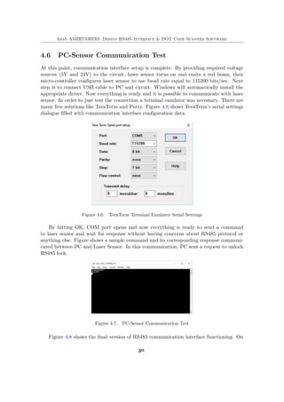
As previously mentioned, in order to run this program again and again for different
newly scanned samples, file name points to "ProfileData.tpd". The ".tpd" extension
has been chosen to the courtesy of Tire Profiles company and stands for Tire Pro-
files Data. According to the previous convention about filling data file, it has one
row of column headers and values are separated by means of tabs. The code for
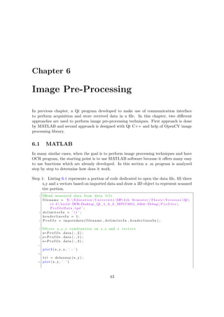
representing x,y and z vectors in 3D format, uses point by point drawing and then
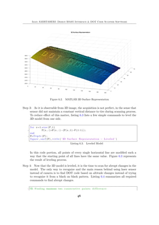
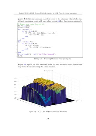
changing the color based on corresponding z value. Figure 6.1 shows output of these
commands, As it is possible to observe the DOT code on tire is "DOT CN3R PY42".
On the right side of this figure, there is a bar showing corresponding color for
different distances. These distances are actually the distances between each point
and laser sensor. For example on right side of tire representation, color dedicated
to characters are less than background color in the sense that the corresponding
distance value is less than the same value for background. Which means the DOT
characters are closer to the laser sensor rather than the background.
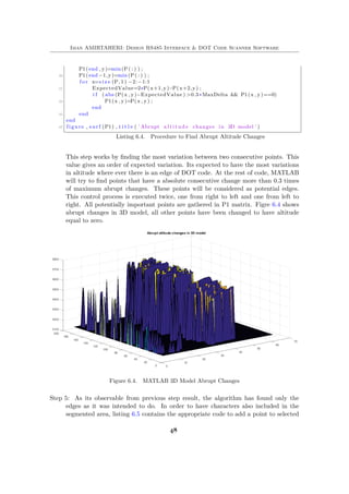
Step 2: For further improvements on achieved results it is a good choice to store x,y
and z vectors inside a matrix called P such a way that x and y values are row and
column indices and z values are stored as matrix elements values. Listing 6.2 lists
all required MATLAB commands to transform x,y,z vectors to P matrix.
1 %Loading Measured data to matrix P
Yindex=0;
3 Xindex=0;
yvalue=−1;
5 f o r i =1: length (x)
i f (y( i )==yvalue )
7 Xindex=Xindex+1;
e l s e
9 Yindex=Yindex+1;
Xindex=1;
11 yvalue=y( i ) ;
end
13 P( Yindex , Xindex )=z ( i ) ;
end
15
44](https://image.slidesharecdn.com/a14ad75b-9842-4ff4-9b4c-90a45f40d9dc-160902161530/85/Thesis-Report-52-320.jpg)
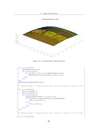
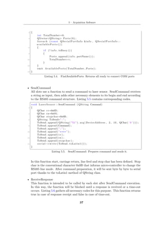
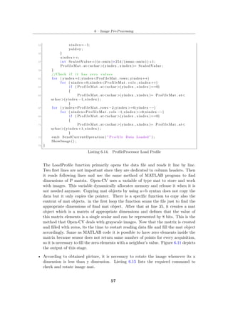
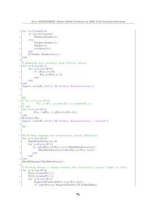
![6 – Image Pre-Processing
Step 7: Now that the 3D manipulation is made effectively by exploiting distance mea-
surement feature, it is possible to convert this 3D model to a normal 2D image to
perform some simple image pre-processing techniques. Listing 6.7 denotes required
commands to perform this important step.
1 % Image Segmentation
P=P ’ ;
3 I = mat2gray (P) ;
mask = f a l s e ( s i z e ( I ) ) ;
5
f o r x=1: s i z e ( I , 1 )
7 f o r y=1: s i z e ( I , 2 )
i f (P(x , y) >=0.9∗max(P( : ) ) )
9 mask(x , y)=true ;
end
11 end
end
13
W = graydiffweight ( I , mask , ’ GrayDifferenceCutoff ’ , 25) ;
15 thresh = 0 . 0 1 ;
[BW, D] = imsegfmm (W, mask , thresh ) ;
17 f i g u r e
imshow (BW)
19 t i t l e ( ’ Segmented BW Image ’ )
Listing 6.7. Image Black & White Segmentation
This step primarily uses a "mat2gray" function to just scale each matrix element value
to have a number between 0 and 255. "mask" variable is used to define a mask which
represents potential seeds of image segmentation. This binary matrix is filled with
ones for points with highest values (above 90%) and zeros for all remaining points.
"graydiffweight" uses the grayscale image and provided mask to calculate a weight
for pixels according to the difference between their value and masked point values.
At the end, "imgsegfmm" function performs segmentation based on the weighted
values, provided mask and a threshold which determines the border of black and
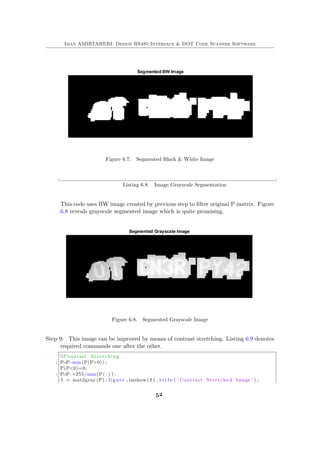
white. Figure 6.7 shows the result of this process.
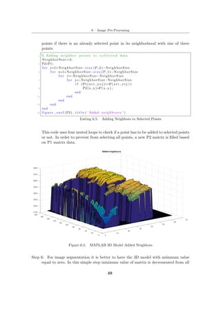
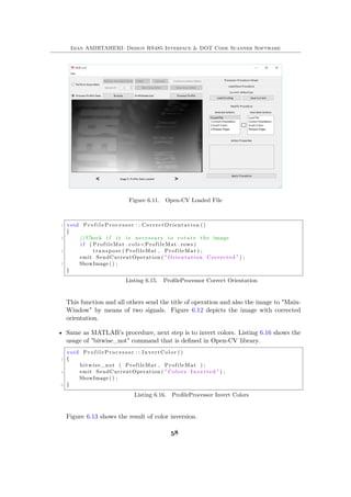
Step 8: It seems that the code has selected the correct region that contains the DOT
code but with current black and white image it is not possible to perform OCR for
sure. So in this step, segmentation mask created by previous step is used to filter
original grayscale image obtained by beginning of previous step.
1 f o r x=1: s i z e ( I , 1 )
f o r y=1: s i z e ( I , 2 )
3 i f (BW(x , y)==f a l s e )
P(x , y) =0;
5 end
end
7 end
I = mat2gray (P) ; figure , imshow ( I ) , t i t l e ( ’ Segmented Grayscale Image ’ )
51](https://image.slidesharecdn.com/a14ad75b-9842-4ff4-9b4c-90a45f40d9dc-160902161530/85/Thesis-Report-59-320.jpg)
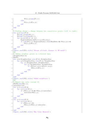
![Iman AMIRTAHERI: Design RS485 Interface & DOT Code Scanner Software
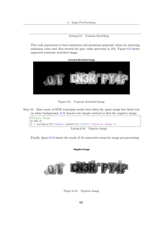
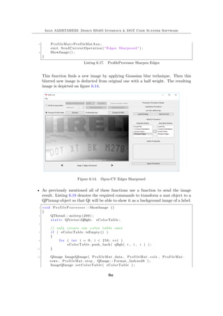
Although this image pre-processing is not perfect but it offers a good approach to make the
3D model clearer for image processing and specifically OCR. Anyway the thesis goal was
mainly to achieve a stable working condition for laser sensor communication and scanner
software acquisition.
6.2 Qt and Open-CV
In previous section, a 10 step pre-image processing algorithm introduced to use with MAT-
LAB program. Since the final program should be developed and deployed with Qt IDE,
although this was not a part of this thesis subject, author tried to implement a few ba-
sic pre-processing algorithms into the scanner Qt C++ software. In this way the field is
widely open for another engineers to expand and make use of it.
Open-CV is an open source computer vision library that supports various operating sys-
tems and programming languages. This flexibility is encouraging programmers to use this
library for their image processing applications. Qt and Open-CV can make a powerful
image processing software since both of them can deploy programs for different operating
systems.[13]
The new Qt software developed along with Open-CV libraries has one more class named
"ProfileProcessor". This class also is defined by files "profileprocessor.h" and "profilepro-
cessor.cpp". Listing 6.11 denotes public and private functions declared by this class.
1 public :
P r o f i l e P r o c e s s o r () ;
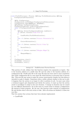
3 void Process ( QString ProfileDataLocation , QString
ConfigurationFileLocation ) ;
private :
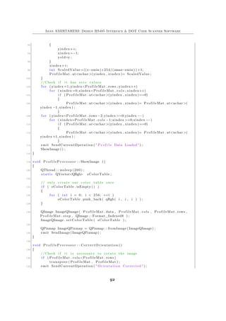
5 void LoadProfile ( QString FileLocation ) ;
void ShowImage () ;
7 void CorrectOrientation () ;
void InvertColor () ;
9 void SharpenEdges () ;
Listing 6.11. ProfileProcessor Functions
In this case there is no advantage to use slots over class functions because the processed
data by the profile processor object should be handled differently than just connecting
it to a user interface element slot. But for signals part, listing 6.12 shows two signals
declared by this class.
1 s i g n a l s :
void SendImage (QPixmap Image ) ;
3 void SendCurrentOperation ( QString Command) ;
Listing 6.12. ProfileProcessor Signals
SendImage and SendCurrentOperation signals, send an image and a descriptive string
respectively. This design is intended in order to make possible to have a good interface in
MainWindow object. Further information will be available later.
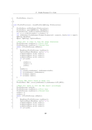
Listing F.1 describes the definition of process function of this class.
54](https://image.slidesharecdn.com/a14ad75b-9842-4ff4-9b4c-90a45f40d9dc-160902161530/85/Thesis-Report-62-320.jpg)


![Bibliography
[1] Michelin Company Canada, Reading A Tire Sidewall, available on-
line at <http://www.michelin.ca/tires-101/tire-basics/about-tires/
reading-your-sidewall.page>
[2] Leith Autopark Kia, September 2014, How To Check Your
Tire Tread for Wear. <http://blog.leithautoparkkia.com/
how-to-check-your-tire-tread-tires-raleigh/>
[3] Tire Profiles LLC, TreadSpec Documents. <http://www.tireprofiles.com/
treadspec/>
[4] Tire Profiles LLC, GrooveGlove Documents. <http://www.tireprofiles.com/
grooveglove/>
[5] TIRE TECH, Determining the Age of a Tire, available online at <http://www.
tirerack.com/tires/tiretech/techpage.jsp?techid=11>
[6] Baumer, BA OM70 MESAX multi-spot. <http://pfinder.baumer.com/pfinder_
sensor/downloads/Produkte/PDF/Allgemein/en_BA_RS485_MESAX_multi-spot_
Commands.pdf>
[7] Baumer, BA RS485 MESAX multi-spot commands,<http://pfinder.baumer.
com/pfinder_sensor/downloads/Produkte/PDF/Allgemein/en_BA_OM70_MESAX_
multi-spot.pdf>
[8] WIKIBOOKS, April 2016, Serial Programming/RS-485. <https://en.wikibooks.
org/wiki/Serial_Programming/RS-485>
[9] Atmel, ATmega16(L) datasheet, available online at <http://www.atmel.com/
images/doc2466.pdf>
[10] Maxminintegrated, MAX481 MAX483 MAX485 MAX487 MAX491 MAX1487,
available online at <https://datasheets.maximintegrated.com/en/ds/
MAX1487-MAX491.pdf>
[11] Prolific Technology Inc., PL-2303HXD Datasheet, available online at http://www.
prolific.com.tw/UserFiles/files/ds_pl2303HXD_v1_4_4.pdf>
[12] Nokia, Qt Documentation, available online at http://doc.qt.io/>
[13] OpenCV, Open Source Computer Vision v3.1.0, http://docs.opencv.org/3.1.0/
#gsc.tab=0>
[14] Kyung, C.M. ed., 2016. Theory and Applications of Smart Cameras. Springer Nether-
lands.
65](https://image.slidesharecdn.com/a14ad75b-9842-4ff4-9b4c-90a45f40d9dc-160902161530/85/Thesis-Report-73-320.jpg)

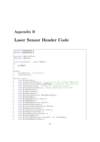
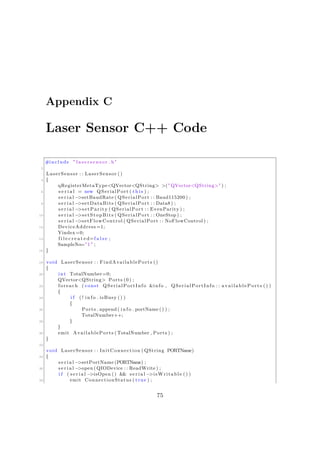
![B – Laser Sensor Header Code
void ReadObjectType () ;
40 void WriteObjectType ( bool Switch ) ;
void ReadPrecision () ;
42 void WritePrecision ( int S e l e c t ) ;
void ReadLaserOffDataHold () ;
44 void WriteLaserOffDataHold ( bool Switch ) ;
void ReadFlexMountEnable () ;
46 void WriteFlexMountEnable ( bool Switch ) ;
void ReadSetFlexMount () ;
48 void WriteSetFlexMount ( f l o a t Angle , f l o a t Distance ) ;
void WriteTeachFlexMountCommand( f l o a t ReferenceThickness ) ;
50 void ReadDiagnoseMode () ;
void WriteDiagnoseMode ( bool Switch ) ;
52 void WriteStoreConfigurationCommand ( int Config ) ;
void WriteResetToFactorySettingsCommand ( int Command) ;
54 void SampleNoChanged ( QString SampleNumber) ;
void CloseConnection () ;
56
s i g n a l s :
58 void AvailablePorts ( int TotalNumber , QVector<QString> Ports ) ; // Searches
f o r a l l a v a i l a b l e COM ports
void ConnectionStatus ( bool Status ) ;
60 void ApplicationError ( int ApplicationError ) ; //Reads a p p l i c a t i o n e r r o r
code
void VendorID ( int Vendor_ID) ;
62 void VendorName( QString Vendor_Name) ;
void DeviceID ( int Device_ID ) ;
64 void VariantID ( int Variant_ID ) ;
void SensorType ( QString Sensor_Type ) ;
66 void SerialNumber ( QString Serial_Number ) ;
void BusAddress ( int BusAddressValue ) ;
68 void BaudRate ( int BuadRateValue ) ;
void RS485Lock ( bool Switch ) ;
70 void TouchButtonLock ( bool Switch ) ;
void MeasurementType ( QString Type) ;
72 void MeasurementValue ( f l o a t MeasurementValue , QString Quality ) ;
void Average ( QString average ) ;
74 void Max ( QString max) ;
void Min ( QString min) ;
76 void Delta ( QString delta ) ;
void StandardDeviation ( QString standarddeviation ) ;
78 void Quality ( QString quality ) ;
void FieldOfView ( int LimitLeft , int LimitRight ) ;
80 void ObjectType ( QString ObjectType ) ;
void Precision ( QString Precision ) ;
82 void LaserOffDataHold ( bool Switch ) ;
void FlexMountEnable ( bool Switch ) ;
84 void SetFlexMount ( f l o a t Angle , f l o a t Distance ) ;
void DiagnoseModeEnabled () ;
86 void P r o f i l e ( int Xpos [ 3 0 0 ] , int Zpos [ 3 0 0 ] ) ;
void SensorTimedOut ( bool Switch ) ;
88 void ProfileReady () ;
90 private :
73](https://image.slidesharecdn.com/a14ad75b-9842-4ff4-9b4c-90a45f40d9dc-160902161530/85/Thesis-Report-81-320.jpg)
![Iman AMIRTAHERI: Design RS485 Interface & DOT Code Scanner Software
e l s e
40 {
emit ConnectionStatus ( f a l s e ) ;
42 }
SendCommand( "W010;0 " ) ;
44 ReceiveResponse () ;
}
46
void LaserSensor : : CheckConnection ()
48 {
50 }
52 void LaserSensor : : ReadApplicationError ()
{
54
}
56
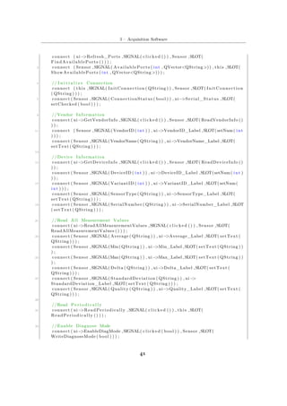
void LaserSensor : : ReadVendorInfo ()
58 {
SendCommand( "R001" ) ;
60 i f ( ReceiveResponse () )
{
62 emit VendorID ( Payloads [ 1 ] . toInt () ) ;
emit VendorName( Payloads [ 2 ] ) ;
64 }
66 }
68 void LaserSensor : : ReadDeviceInfo ()
{
70 SendCommand( "R002" ) ;
i f ( ReceiveResponse () )
72 {
emit DeviceID ( Payloads [ 1 ] . toInt () ) ;
74 emit VariantID ( Payloads [ 2 ] . toInt () ) ;
emit SensorType ( Payloads [ 3 ] ) ;
76 emit SerialNumber ( Payloads [ 4 ] ) ;
}
78 }
80 void LaserSensor : : ReadBusAddress ()
{
82
}
84
void LaserSensor : : WriteBusAddress ( int BusAddressValue )
86 {
88 }
90 void LaserSensor : : ReadBaudRate ()
{
92
76](https://image.slidesharecdn.com/a14ad75b-9842-4ff4-9b4c-90a45f40d9dc-160902161530/85/Thesis-Report-84-320.jpg)
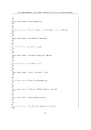
![C – Laser Sensor C++ Code
}
94
void LaserSensor : : WriteBaudRate ( int S e l e c t )
96 {
98 }
100 void LaserSensor : : ReadRS485Lock ()
{
102
}
104
void LaserSensor : : WriteRS485Lock ( bool Switch )
106 {
108 }
110 void LaserSensor : : ReadTouchButtonLock ()
{
112
}
114
void LaserSensor : : WriteTouchButtonLock ( bool Switch )
116 {
118 }
120 void LaserSensor : : ReadMeasurementType ()
{
122
}
124
void LaserSensor : : WriteMeasurementType ( int S e l e c t )
126 {
128 }
130 void LaserSensor : : ReadMeasurementValue ()
{
132
}
134
void LaserSensor : : ReadAllMeasurementValues ()
136 {
SendCommand( "R022" ) ;
138 i f ( ReceiveResponse () )
{
140 emit Average ( Payloads [ 1 ] ) ;
emit Max( Payloads [ 2 ] ) ;
142 emit Min( Payloads [ 3 ] ) ;
emit Delta ( Payloads [ 4 ] ) ;
144 emit StandardDeviation ( Payloads [ 5 ] ) ;
emit Quality ( Payloads [ 6 ] ) ;
146 }
77](https://image.slidesharecdn.com/a14ad75b-9842-4ff4-9b4c-90a45f40d9dc-160902161530/85/Thesis-Report-85-320.jpg)
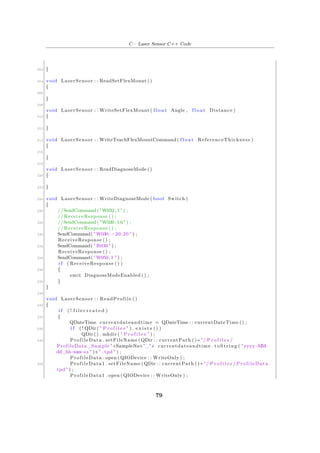
![Iman AMIRTAHERI: Design RS485 Interface & DOT Code Scanner Software
252 ProfileStream . setDevice(&ProfileData ) ;
ProfileStream << "YtX t Z" <<endl <<endl ;
254 ProfileStream1 . setDevice(&ProfileData1 ) ;
ProfileStream1 << "YtX t Z" <<endl <<endl ;
256 f i l e c r e a t e d=true ;
}
258 SendCommand( "R052" ) ;
i f ( ReceiveResponse () )
260 {
i f ( Payloads [ 0 ] . contains ( "A" ) )
262 {
QStringList XZMeasurements ;
264 XZMeasurements=Payloads [ 2 ] . s p l i t ( " " ) ;
int TotalMeasurements=XZMeasurements [ 0 ] . toInt () ;
266 XZMeasurements . removeFirst () ;
Yindex++;
268 f o r ( int i =0; i<TotalMeasurements /2; i++)
{
270 ProfileStream << Yindex <<" t " << XZMeasurements [2 ∗ i ] <<" t "
<<XZMeasurements [2 ∗ i +1] <<endl ;
ProfileStream1 << Yindex <<" t " << XZMeasurements [2 ∗ i ] <<" t
" <<XZMeasurements [2 ∗ i +1] <<endl ;
272 }
emit ProfileReady () ;
274 }
e l s e
276 {
qDebug ()<<" Error Handling "<<Payloads [ 0 ] ;
278 i f ( Payloads [1]== " 7 " )
WriteDiagnoseMode ( true ) ;
280 e l s e
ReadProfile () ;
282 }
}
284 e l s e
emit ProfileReady () ;
286 }
288 void LaserSensor : : WriteStoreConfigurationCommand ( int Config )
{
290
}
292
void LaserSensor : : WriteResetToFactorySettingsCommand ( int Command)
294 {
296 }
298 void LaserSensor : : CloseConnection ()
{
300 Yindex=0;
ProfileData . c l o s e () ;
302 ProfileData1 . c l o s e () ;
f i l e c r e a t e d=f a l s e ;
80](https://image.slidesharecdn.com/a14ad75b-9842-4ff4-9b4c-90a45f40d9dc-160902161530/85/Thesis-Report-88-320.jpg)

![Appendix D
Profile Processer MATLAB Code
1 c l c
c l e a r
3 c l o s e a l l
5 %Read measured data from data f i l e
filename = ’E: Education University MS4 th Semester Thesis Versions Qtv1 .6
build−DCR−Desktop_Qt_5_6_0_MSVC2015_64bit−Debug P r o f i l e s ProfileData . tpd ’
;
7 d e l i m i t e r I n = ’ t ’ ;
headerlinesIn = 1;
9 P r o f i l e = importdata ( filename , delimiterIn , headerlinesIn ) ;
11 %Store x , y , z combination on x , y and z vectors
x=P r o f i l e . data ( : , 2 ) ;
13 y=P r o f i l e . data ( : , 1 ) ;
z=P r o f i l e . data ( : , 3 ) ;
15
plot3 (x , y , z , ’.− ’ )
17
t r i = delaunay (x , y) ;
19 plot (x , y , ’ . ’ )
21 [ r , c ] = s i z e ( t r i ) ;
disp ( r )
23
h = t r i s u r f ( t r i , x , y , z ) ;
25 axis vis3d
axis o f f
27 l = l i g h t ( ’ Position ’ ,[ −50 −15 29 ] ) ;
set ( gca , ’ CameraPosition ’ ,[208 −50 7687]) ;
29 l i g h t i n g phong
shading interp
31 colorbar EastOutside
33 %Loading Measured data to matrix P
Yindex=0;
35 Xindex=0;
yvalue=−1;
83](https://image.slidesharecdn.com/a14ad75b-9842-4ff4-9b4c-90a45f40d9dc-160902161530/85/Thesis-Report-91-320.jpg)
![Iman AMIRTAHERI: Design RS485 Interface & DOT Code Scanner Software
145 P=P2 ;
147 % % Saturated Levels
% P(P>mean(P( : ) ) )=mean(P( : ) ) ;
149 % figure , s u r f (P) , t i t l e ( ’ Homogenized Levels ’ )
%%
151 % Image Segmentation
P=P ’ ;
153 I = mat2gray (P) ;
mask = f a l s e ( s i z e ( I ) ) ;
155
f o r x=1: s i z e ( I , 1 )
157 f o r y=1: s i z e ( I , 2 )
i f (P(x , y) >=0.9∗max(P( : ) ) )
159 mask(x , y)=true ;
end
161 end
end
163
W = graydiffweight ( I , mask , ’ GrayDifferenceCutoff ’ , 25) ;
165 thresh = 0 . 0 1 ;
[BW, D] = imsegfmm (W, mask , thresh ) ;
167 f i g u r e
imshow (BW)
169 t i t l e ( ’ Segmented BW Image ’ )
%%
171 f o r x=1: s i z e ( I , 1 )
f o r y=1: s i z e ( I , 2 )
173 i f (BW(x , y)==f a l s e )
P(x , y) =0;
175 end
end
177 end
I = mat2gray (P) ; figure , imshow ( I ) , t i t l e ( ’ Segmented Grayscale Image ’ )
179
181 % % Modifying each l i n e a l t i t u d e to have same max value f o r a l l l i n e s
% P=P ’ ;
183 % maxaltitude=max(P( : ) ) ;
% f o r y=1: s i z e (P, 2 )
185 % P( : , y)=P( : , y) ∗ ( maxaltitude /max(P( : , y) ) ) ;
% end
187 % figure , s u r f (P) , t i t l e ( ’ Modified Image to have same max value f o r each line
’ )
% P=P ’ ;
189
%P=P. ^ 5 ;
191 %figure , s u r f (P)
193
195
%
197 I = mat2gray (P) ; figure , imshow ( I )
86](https://image.slidesharecdn.com/a14ad75b-9842-4ff4-9b4c-90a45f40d9dc-160902161530/85/Thesis-Report-94-320.jpg)


![wronski_ugthesis[1]](https://cdn.slidesharecdn.com/ss_thumbnails/95db93fc-5f15-4802-985f-832034d277d7-150202014804-conversion-gate02-thumbnail.jpg?width=640&height=640&fit=bounds)


