This document is a master's thesis submitted by Milan Tepić to the University of Stuttgart exploring host-based intrusion detection to enhance cybersecurity in real-time automotive systems. The thesis was supervised by Dr.-Ing. Mohamed Abdelaal and examined by Prof. Dr. Kurt Rothermel. It explores using timing elements of control unit functions to detect anomalies and intrusions. The goal is to develop a host-based intrusion detection system called AutoSec that can detect anomalies while keeping false alarms close to zero, in compliance with the AUTOSAR automotive software standard.


![Abstract
Modern automotive industry develops technology advancing vehicles in direction of inter-
connectivity. Estimation forecast [1] shows that by 2025, more than 470 million vehicles
will be connected among each other, to Smart-Roads, Smart-Homes, etc. Due to external
communication of a car to surrounding, the vehicle is under the exposure to potential attacks
through those communication channels. The attack case from 2015. by C. Miller and C.
Valasek [2] shows what could happen if modern vehicles are not protected from external
malicious/non-verified access. In order to detect an attack, an Intrusion Detection System
(IDS) is used. However, the future attacks cannot be predicted, and thus IDS are run to detect
anomalies in the system behavior. IDS can be separated into two main fields: Communication
channels monitored by Network-based IDS and Control Units monitored by Host-based IDS.
The scope of the Thesis is detecting anomalies of behavior of a Control Unit within the vehicle
based on timing elements of its functions. The method proposed by this Thesis is called
AutoSec - Host-based Intrusion Detection System. The goal of AutoSec is, in compliance with
AUTOSAR standard, to reach high detection rate of Anomalies in the system, by keeping
level of False Alarms close to zero.
iii](https://image.slidesharecdn.com/milanthesis-220913145214-138d4713/75/Milan_thesis-pdf-7-2048.jpg)


![List of Figures
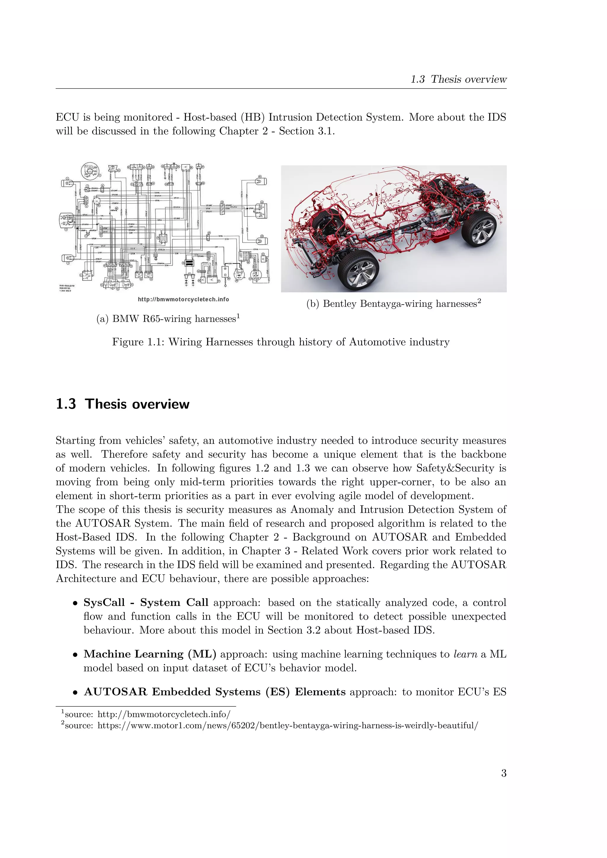
1.1 Wiring Harnesses through history of Automotive industry . . . . . . . . . . . . 3
1.2 Vector Client Survey 20171 . . . . . . . . . . . . . . . . . . . . . . . . . . . . . 4
1.3 Vector Client Survey 20182 . . . . . . . . . . . . . . . . . . . . . . . . . . . . . 4
2.1 Cohesion vs Coupling of software structure [3] - slide 326 . . . . . . . . . . . . 8
2.2 AUTOSAR Releases3 . . . . . . . . . . . . . . . . . . . . . . . . . . . . . . . . . 9
2.3 AUTOSAR Layered architecture organization - simplified representation . . . . 10
2.4 AUTOSAR - Application Layer [4] . . . . . . . . . . . . . . . . . . . . . . . . . 11
2.5 Basic Software (BSW) Structure [5] . . . . . . . . . . . . . . . . . . . . . . . . 12
2.6 Queue of ready tasks waiting for execution[6] . . . . . . . . . . . . . . . . . . . 15
2.7 Example of a preemptive schedule[6] . . . . . . . . . . . . . . . . . . . . . . . . 15
2.8 Precedence relations among five tasks [6] . . . . . . . . . . . . . . . . . . . . . . 18
2.9 Precedence relations causing J5 to miss the deadline4 . . . . . . . . . . . . . . . 19
2.10 Structure of two tasks that share a mutually exclusive resource protected by a
semaphore [6] . . . . . . . . . . . . . . . . . . . . . . . . . . . . . . . . . . . . . 20
2.11 Task’s state diagram [6] . . . . . . . . . . . . . . . . . . . . . . . . . . . . . . . 20
2.12 Graphical representation of the Table 2.1 . . . . . . . . . . . . . . . . . . . . . 23
2.13 AUTOSAR Example of Top-Down development approach [7] . . . . . . . . . . 24
2.14 AUTOSAR Example of Data floww in the scope of the VfbTiming view [8] . . 27
2.15 AUTOSAR Example of Data floww in the scope of the SwcTiming view [8] . . 27
3.1 Different approaches on Intrusion Detection Systems . . . . . . . . . . . . . . . 30
3.2 [9] - Trace tree generated from a sequence of traces . . . . . . . . . . . . . . . . 34
3.3 [9] - Probability density estimation of an example execution block . . . . . . . . 35
3.4 Probability density function on two dimensional random variable X(S2S, computation) 36
4.1 Typical timing parameters of a Real-Time Task τi - previously explained in
Section 2.2.2 . . . . . . . . . . . . . . . . . . . . . . . . . . . . . . . . . . . . . 38
4.2 Example of Execution Diagram using TA Tool Suite [10] . . . . . . . . . . . . . 38
4.3 Example of 2D feature space: Start-to-Start (S2S) vs. Computation time . . . 41
4.4 Example of 2D feature space: Computation time vs. Npreemptions . . . . . . . . 42
4.5 Example of 3D feature space: S2S vs. Computation time vs. Npreemptions . . . 43
4.6 Example of 4D feature space after Principal component analysis (PCA): S2S
vs. Computation time vs. Npreemptions vs τpreemptions . . . . . . . . . . . . . . . 44
4.7 Histogram distribution of two features [Upper-left and bottom-right subfigures]
Computation time needed by Measuring point over time[bottom-left subfigure]
Overlapped distributions of feature 1 and feature 2 with each data point pre-
sented as a square in 2D feature space [upper-right subfigure] . . . . . . . . . . 47
vii](https://image.slidesharecdn.com/milanthesis-220913145214-138d4713/75/Milan_thesis-pdf-11-2048.jpg)


![Chapter 1
Introduction
Modern life experiences rapid evolution and sudden changes on daily basis. Technological
capabilities are there to help us while residing in the background of our lives. Looking back
into last 2 decades, we can observe an influence of technology. 20 years back, mobile network
had very little coverage in comparison to today’s capabilities. 10 years later, the first smart
phones started becoming part of our lives. Today we witness a new element that is about to
become the next part of us.
Upcoming 5G mobile network brings new technological innovations resulting in a multi-billion
number of interconnecting devices. Considering part of these devices is related to the trans-
portation system, mainly new smart cars with autonomous driving systems, smart roads,
etc. According to Ericsson, one of the biggest telecommunication vendors in the World, around
400 million devices have been interconnected with cellular connection as part of Internet of
Things (IoT). Furthermore, the number of these devices exponentially grows and estimations
show that the number of networked devices will overcome 1.5 billion by 2022 [11]. Personal
transportation vehicles are part of this network and we can already get hands on one of
those state-of-art vehicles, such as Tesla - Connectivity, Mercedes-Benz - me connect, BMW
- Connect Drive, etc. The main focus is rather way broader than only a connection to the
Network. News as [12] confirm merging actions of multiple Automotive Original Equipment
Manufacturer (OEM)s, regarding services based on inter-connectivity.
1.1 General Problem Statement
Considering the automotive industry, when it comes to vehicles and passengers, the safety is
the top priority. One of the most important standards is ISO26262, titled Road vehicles –
Functional safety, being the core of modern automotive industry [13]. In order to enhance
the safety of passengers while enriching their drive comfort, vehicle-to-vehicle (known as V2V),
or generally speaking Car2X (car-to-many), is there to interconnect the traffic and support
sharing of valuable information about the surrounding, road cases, safety warnings, etc. The
topic of Car2X is discussed in [14], followed by an example regarding the average drivers’
reactions and the travelled distance during this short time. Driver’s reaction time is defined
as the time between when the event has been observed and the time at which the driver
actually reacts. Typical reaction time is in the range from 0.75 to 1.5 s [15]. The traveled
distance during the reaction time, at the speed of 110 km/h, is between 23 and 46 m. Hence,
1](https://image.slidesharecdn.com/milanthesis-220913145214-138d4713/75/Milan_thesis-pdf-21-2048.jpg)
![1 Introduction
the need for connecting cars in order to improve safety systems, increases. Side effect results
in opening modern vehicles’ systems to be exposed to external threats from cyberattacks.
1.2 Motivation
Historically, very first cars had close to nothing technicalities related to the electronics, apart
from basic wiring harnesses. One of the examples can be seen in the Figure 1.1a, where the
wiring harnessing for BMW R65 is presented. Fundamentally, the only electronics necessar-
ily needed for running the car are related to engine and accumulator connections. However,
safety in traffic and commuting raised concerns and at first, turning signals have been added,
then wipers, etc. Additional safety measures and comfort features and systems raised the
complexity level of wiring systems in modern cars. The complexity, only of wiring, has been
showed in the Figure 1.1b.
According to [16], premium cars in 2010 had up to 70 Electronic Control Unit (ECU), while
today this number has gone beyond 100. The ECU is a computational unit that is in charge of
specific control and handling of a vehicle elements, such as engine control, suspension control,
driver assistance (i.e. Advanced driver-assistance systems (ADAS)), etc. Thus, considerable
level of innovations (90%) in automotive industry is driven by electronics and software. There-
fore, the development costs of electronics and software are going up to 40% of all costs, while
50-70% of these costs are invested in software for ECUs.
Considering this amount of control units (ECUs), we have a distributed multivariable sys-
tem. These units used to communicate over Controll Area Network (CAN), developed in
’80s specifically for automotive industry. With increased number of data needed for complex
control and calculations, modern cars implement Ethernet communication as well. All of this
has made modern vehicles to be considered as big computational units. Due to this high
level of complexity and dependencies, a partnership between main OEMs and Tier1 suppliers
has been organized to standardize modern vehicle architecture. The AUTOSAR has been
grounded in 2002-2003 [17]. The first release AUTOSAR Classic Platform Release 1.0 was in
2005. More about AUTOSAR will be discussed in the Chapter 2 - Section 2.1.1 AUTOSAR.
Due to increasing number of safety systems and their complexity, there is a high internal
communication overhead. Influenced by IoT and interconnectivity requirements, the internal
communication in cars has been exposed to attackers more than ever. The most well known
an attack on a vehicle network has been performed by Charlie Miller and Chris Valasek [2].
They have breached into the vehicle network and interfered the messages payloads. By these
doings, Miller and Valasek were able to completely overtake the control over the vehicle. The
greatest concern was that they have been able to override drivers action remotely through
wireless network by being many kilometers away from the vehicle.
Following this event, many OEMs started rapid investments in security measures of vehi-
cle’s electronics and software, resulting in increasing number of researches about Intrusion
Detection System (IDS). The scope of vehicle protection is not only based on protecting com-
munication between ECUs, but also to protect internal components and integrity of each ECU
separately. The main classification of IDS is based on whether a Network/Communication
is monitored - Network-based (NB) Intrusion Detection System; or a internal operations of
2](https://image.slidesharecdn.com/milanthesis-220913145214-138d4713/75/Milan_thesis-pdf-22-2048.jpg)


![Chapter 2
Background
The transportation and commuting has become important part of our lives. Therefore, the
automotive industry is developing high measures of safety and nowadays security measures
for modern vehicles. In addition, in order to make commuting comfortable and extremely
pleasant, new technologies for autonomous driving are in a fast development process. As
described in [18], the automotive industry has an aim to replace human perception of the
environment. Thus, the modern technologies as high-resolution radar and video sensors are
essential in order to bring new driver assistance systems in use. Due to high sensor resolu-
tions and high data sampling rate, excessive amount of data has been transported via vehicle’s
communication networks. In addition to communication, all the data needs to be processed
in real-time so the needed and required safety is guaranteed. Many different challenges in this
complex architecture [19] occurs and they need to be standardized. The main focus today is
as discussed in Section 1.2 - Motivation.
ADAS is the main component in today’s vehicles which ensures the assistance to the driver
and ease of driving while guarantying safety of all passengers and other actors in the surround-
ing. The most common safety elements are: ACC - Adaptive Cruise Control, LDW - Lane
Departure Warning, EBA - Emergency Brake Assist, BSD - Blind Spot Detection, RCTA -
Rear Cross Traffic Alert, etc. The extreme number of vast sensors and actuators require high
computational power and control to ensure given requirements, especially in terms of safety.
2.1 Operating Systems
Based on the requirements, a deterministic system with time constraints is needed to ensure
designed control and data flow needed for safety guarantees. Thus, ES as Real-Time Sys-
tem (RTS) are widely used in automotive industry to provide needed determinism. More about
Real-Time (RT) Systems and Constraints, refer to Section 2.2 - Real-Time Systems. With
the complexity of vehicle’s Electric and Electronic (E/E) Systems, ES needed standardization
in automotive industry. Many vehicle manufacturers use Automotive Grade Linux (AGL) as
underlying Operating System (OS) to ensure Real-Time Constraints. Some other OEMs use
Real-Time Operating System (RTOS) such as QNX, FreeRTOS, OpenRTOS, etc.
However, standardized automotive architecture is AUTOSAR - AUTomotive Open System
ARchitecture. AUTOSAR is an alliance of OEMs, Tier1 suppliers, semiconductor manufac-
turers, software suppliers, tool suppliers and others organized to establish an open industry
7](https://image.slidesharecdn.com/milanthesis-220913145214-138d4713/75/Milan_thesis-pdf-27-2048.jpg)
![2 Background
Figure 2.1: Cohesion vs Coupling of software structure [3] - slide 326
standard for an automotive software architecture. The main purpose is to define a basic in-
frastructure for the management of functions within both future applications and standard
software modules [17].
2.1.1 AUTOSAR
In 2003, automotive OEMs, Tier1 suppliers and related manufacturers and suppliers joined
on the mission to develop the basis of future software for ECUs in vehicles - AUTOSAR.
The aim is to create a backbone for collaboration on basic functions, whilst excluding certain
functional components of higher level of abstraction. The components were left out for making
a competitiveness in development and innovations, between different suppliers, in terms of new
functions and features. The core advantage of AUTOSAR is an ability to flexibly distribute
software into ECUs, independently of a ECU supplier or hardware architecture.
Summing up, as explained in [4], AUTOSAR goals are as follows:
• Standardization of interfaces between functions of the application software and to basic
functions
• Definition of a reference architecture for ECU software
• Standardization of exchange formats for distributed development processes
Since automotive industry has dominant attributes of innovation and competitiveness, there
are multiple benefits introduced by using AUTOSAR:
• Ability to optimize the ECU network by flexible integration, relocation and exchange of
8](https://image.slidesharecdn.com/milanthesis-220913145214-138d4713/75/Milan_thesis-pdf-28-2048.jpg)
![2.1 Operating Systems
functions
• Mastery over increasing product and process complexity
• Maintainability over entire product life cycle
By excluding specifications and requirements regarding certain components in AUTOSAR
due to competitiveness and innovations, the AUTOSAR standard lacks the capability of de-
scribing the functional behavior of a software components. Contrary to being a disadvantage,
this lack of capability helps to reach higher modularity. As explained in [3], the main goal
of modularity is high cohesion and low coupling of the software structure. With respect
to the code units, cohesion represents intramodule connectivity and coupling represents in-
termodule connectivity - Figure 2.1. Since 2003, AUTOSAR Alliance has released 4 versions,
called Releases. The year and a release version of AUTOSAR can be followed through the
Figure 2.2. Meanwhile, AUTOSAR Version 3.0 was the first release used in production line
ECUs.
Figure 2.2: AUTOSAR Releases1
1
source: https://elearning.vector.com/mod/page/view.php?id=439
9](https://image.slidesharecdn.com/milanthesis-220913145214-138d4713/75/Milan_thesis-pdf-29-2048.jpg)
![2 Background
2.1.1.1 Concept
AUTOSAR specifications, templates, requirements and other related documents can be found
on the official page of alliance - AUTOSAR Official Website. According to general specifica-
tion of the AUTOSAR, the Architecture distinguishes on the highest abstraction level between
three software layers: Application, Real-Time Environment (RTE) and BSW which run on a
Microcontroller or Microcontroller Abstraction Layer (MCAL), as presented in the Figure 2.3
[5].
• Application Layer - OEM defined applications and use cases, i.e. Anti-lock Braking
System (ABS), control of Daytime Lights, control of Windows on doors, etc.
• RTE - abstracts the application layer from the basic software. It controls the runtime
behavior of the application layer and implements the data exchange [4].
• BSW - many predefined modules that are grouped into layers. For detailed structure
and organization of BSW refer to Section 2.1.1.2.
• Microcontroller Layer - specific firmware dependent on ECU architecture. It is provided
by hardware vendors.
Figure 2.3: AUTOSAR Layered architecture organization - simplified representation
2.1.1.2 Architecture
Through this section, two main Layers will be considered - Application Layer and Basic
Software Layer. As it will be discussed in Chapter 3 and 4, elements and features of these
two layers will be used.
Having an insight on more fine-granular level, the Application Layer consists of different
Applications. As it could be seen in the Figure 2.4a (different applications are Left Door,
Right Door and Door Contact. In the first steps during a design, the functional software
of the vehicle is described in a high abstraction layer, as it could have been seen in the
10](https://image.slidesharecdn.com/milanthesis-220913145214-138d4713/75/Milan_thesis-pdf-30-2048.jpg)
![2.1 Operating Systems
Figure 2.4a. Following next lower level of abstraction, the overall system is divided into sub-
functionalities. Mainly, each of this applications consists of different functional blocks called
Software Component (SWC) - Figure 2.4b.
Applications does not necessarily consists of a single SWC but rather of multiple SWC. A
SWC can be either SWC-Composition or SWC-Atomic. The difference is that Atomic could
not be further divided in terms of functionalities, while Composition consists of other SWC-
Compositions and/or SWC-Atomics.
Having a look into the structure of a SWC, building blocks of a SWC are called Runnables
(Runnable Entities). In other words, as described in [4], Runnable Entity is the execution unit,
which is finally implemented as a C function, as it is depicted in Figure 2.4c. The function
calls to the Runnable Entities are configured by the developer, and later implemented by the
RTE. This might, for example be periodic or spontaneously in response to receiving a data
element.
The distinctive feature of SWC is the communication abstraction between multiple SWCs
through interfaces. The Data is transmitted through RTE over Virtual Functional Bus (VFB)
to some other SWC(s). The communication interfaces provide Ports as an attaching elements
for a communication between multiple entities. The Port description is agreed prior to the
design of SWC, so all developers of different Applications know the Communication Policies.
Mainly, AUTOSAR distinguish between two different methods of communication: Sender-
Receiver and Client-Server. For more about these methods refer to [20].
(a) Applications example
(b) Mappings to SWC
(c) SWC mapped on Runnables
Figure 2.4: AUTOSAR - Application Layer [4]
11](https://image.slidesharecdn.com/milanthesis-220913145214-138d4713/75/Milan_thesis-pdf-31-2048.jpg)
![2 Background
As it will be discussed in the following Section 2.3, Application Layer is OEM dependent,
while BSW is provided and designed by the specific vendor of AUTOSAR. The layer model
simplifies porting of software to different hardware. Previously, such porting required extensive
adaptations at various points all the way up to the application layer in the case of poorly
designed software architectures. Using AUTOSAR, all what needs to be done is to replace all
microcontroller specific drivers in the MCAL. The modules in the ECU abstraction layer just
need to be reconfigured whilst all other layers not being affected by porting. This significantly
reduces implementation and testing effort as well as associated risk. The main course of this
Thesis is to cover safety of the system from the point of BSW. Basic Software can be divided
into four main components [5], as presented in the Figure 2.5.
Figure 2.5: BSW Structure [5]
The Service Layer presents the highest layer of the Basic Software whose task is to provide
basic services for Applications, RTE and Basic Software Modules. Services provided by this
sub-layer reflect standardized services related to Operating System, Memory, Network com-
munication, etc. The main Services are: System Service, Memory Services, Crypto Services,
Off-board Communication Services, Communication Services.
The Electronic Control Unit Abstraction Layer (ECUAL) offers uniform access as an interface
to MCAL, all functionalities of an ECU such as communication, memory or IO – regardless of
whether these functionalities are part of the microcontroller or are implemented by peripheral
components. The target of this layer is to make higher software layers independent of ECU
hardware layout.
The Microcontroller Abstraction Layer (MCAL) is the lowest software layer in the BSW as a
layer containing internal drivers for direct access to microcontroller and internal peripherals,
such as: access to memory, communication, input/output (IO) of the microcontroller, etc.
The goal is to make higher software layers independent of microcontroller
The Complex Drivers Layer (Complex Driver(s) (CDD)) spans from the hardware to the RTE.
The CDD layer is a special case for special purpose functionalities, as drivers for devices, that
are not specified within AUTOSAR, for migration purposes, or for drivers with very high
timing constraints.
12](https://image.slidesharecdn.com/milanthesis-220913145214-138d4713/75/Milan_thesis-pdf-32-2048.jpg)
![2.2 Real-Time Systems
2.2 Real-Time Systems
System Engineering is highly broad field of study. Mainly, if the system needs to be always
on and ready to react on external stimulus, the system is considered Real-Time System.
The explanation of Real-Time systems is given in [6]. The Real-Time systems are not about
systems that depend only on a value or data, but rather depending more on those values being
on time as for calculation processes being executed in time. A reaction happening too late
could lead to severe consequences. Severity in this context is related to safety of the system.
More about Safety and Security of such systems will be discussed in following Section 3.1.
The definition of Safety and Security is given in [21]:
• Definition of Safety: “Safety is the state of being ‘safe’ (from French sauf), the
condition of being protected from harm or other non-desirable outcomes”
• Definition of Security: “A system is secure if it is protected against harm caused by
attacks originating from outside the system.”
Depending on timing criticality, a system can be Soft- or Hard-Real Time System. The main
difference is in severity of consequences if a deadline of a task in the real-time system has been
missed. In order to secure the constraints of Safety and Security, Real-Time computations is
needed. More about Timings in Real-Time Systems will be discussed in the following Section
2.2.2. The ubiquitous presence of Real-Time Embedded Systems within everyday applications
that we use will be presented in Section 2.2.4 as part of the motivations of this Thesis.
2.2.1 Fundamentals of Real-Time Embedded Systems
The wide range of today’s applications are developed as Real-Time systems due to high need
of different in time processes. Timing criticality, in order to ensure SafetySecurity, needs
deterministic behaviour and high level of certainty in execution context. The certainty in
execution is being guarded by specifying Deadlines. Depending on the Deadline, soft and
hard deadlines can be distinguished, differentiating a Soft Real-Time System from the Hard
Real-Time System. The definition of hard deadline as a time constraint is [21]:
• Definition of Time Constraint: “A time constraint is called hard if not meeting that
constraint could result in a catastrophe.”
Each system consists of different states of the executions, applications, elements, processes,
etc. One of the examples is given in previous Chapters as the Control Systems in Automotive
Industry and AUTOSAR being one of the elements of a system, of the vehicle. A process is
a computation executed on the processor. The process as a logical unit with specified goal to
be executed is called Task. During a lifetime of a system, the Task will be executed indefinite
number of times. Each instance of a Task is called Job. The order of Jobs, meaning the order
of Tasks’ executions is calculated using a Scheduler. A scheduler is a computational unit
13](https://image.slidesharecdn.com/milanthesis-220913145214-138d4713/75/Milan_thesis-pdf-33-2048.jpg)
![2 Background
which calculates when an instance of a Task will be scheduled for an execution. The calculation
is based on timing constraints of Tasks and also dependent on a scheduling algorithm. More
about specifics regarding Tasks, Jobs and Scheduler refer to [21]. In the following chapters,
the elements that will be discussed are related to the understanding of the AUTOSAR OS
and AutoSec, an intrusion detection concepts proposed in this Thesis.
In this section, tasks and tasks’ timings used for designing an embedded system will be
discussed. Firstly, a different types of tasks need to be differentiated. Mainly, depending on
the nature of the Task, we differ three types of Tasks [6]:
• Periodic Task - tasks in embedded systems are commonly periodic, meaning that
each task has the period of execution. The example is sampling data from a sensor.
The required sampling rate is 1kHz, therefore a Task that reads sensor data will be
triggered/called every 1/1kHz = 1ms.
• Sporadic Task - not as common as periodic tasks in embedded systems. The sporadic
tasks usually do not have the period of execution, but rather an expected minimum
interarrival time, meaning only probability of time between two instances of the sporadic
task is specified. The example, occasional checkup of the system network, driven by some
internal or external events, timeouts or actions.
• Aperiodic Task - the aperiodic task is very similar to the sporadic task, but the
difference is that the aperiodic tasks do not have specified minimum interarrival time.
The aperiodic task are only a specific reaction to the certain action in the system. The
example could be: activation of the ABS in the car, or activation of Air-Bags in the car
when a collision occurs.
During the design time, for each task an execution time will be calculated, usually based on
Worst-Case Execution Time (WCET) calculations. By knowing expected execution time and
a period of periodic tasks, an overall expected Central Processing Unit (CPU) load - processor
utilization can be calculated [6], as shown in the equation:
U =
n
X
i=1
ci
pi
(2.1)
In the Equation 2.1, n is the number of tasks mapped to the processor, while ei is the execution
time of a certain task and pi is the period of that task. In the literature, execution time can
be also denoted as Ci or ci as a computation time of a task, while a period can be denoted as
Ti as task execution.
In a system, processes are not equally important for the functionality of a system. The
example in automotive industry could be: controlling values for proper engine functioning is
more important than sending the control value for turning signal at the same given moment.
Therefore, if two tasks are ready to be executed at the same time, a more important task has
higher priority. Due to that fact, each task has its priority level denoted as capital P, Pi. Note
that order of priority levels depends on the implementation of the OS of Embedded System,
i.e. smaller priority number presents higher priority, or vice verse.
14](https://image.slidesharecdn.com/milanthesis-220913145214-138d4713/75/Milan_thesis-pdf-34-2048.jpg)
![2.2 Real-Time Systems
Depending on the scheduling algorithm, task priorities can be statically assigned during a
design time or dynamically during a runtime. In a case of AUTOSAR, for reaching high level
of determinism, a static priority assignment is used. During an execution of a Job, some
other Job of higher priority Task can be released for an execution. At that moment, without
additional constraints related to resource access controls, the Job of higher priority class,
denoted as JH, will preempt the Job of lower priority Task, denoted as JL. Thus, the job
JH will start its execution immediately while the job JL will wait until all jobs of tasks with
higher priority have finished their executions, since the job JH can be furthermore preempted
by another job of a task with even higher priority than JH has. Scheduling concept of task
with preemption is given in Figure 2.6. The example of Jobs execution with preemption is
presented using Gannt chart approach and it is presented in the Figure 2.7. Note that, in this
example, provided by [6], priorities are P3 P2 P1, where P3 is priority level of J3, and the
same for jobs J2 and J1, respectively. In the lower graph in Figure 2.7, using σ(t) is denoted
current priority level of a Task being executed.
Figure 2.6: Queue of ready tasks waiting for execution[6]
Figure 2.7: Example of a preemptive schedule[6]
15](https://image.slidesharecdn.com/milanthesis-220913145214-138d4713/75/Milan_thesis-pdf-35-2048.jpg)
![2 Background
However, sometimes preemption can be turned off during a runtime. The occasion of such
action is related when a Task has an access to a shared resource, or has an execution of
a critical section. The example of a shared resource is a memory, variable in a memory
location. In order to keep data consistence, only one Task can have an access to the memory
(location) at the time. Regarding the critical section, example could be reading/writing a
data stream from/to a communication channel and any interruption of the execution can lead
to a communication error or a malfunction, i.e. I2C communication line being blocked2.
These severity of any ambiguity of the system that can happen during a runtime needs to be
considered during a design time. The verification of the system consistency and certainty is
done by evaluating timings of the system. Common timings used for the evaluation of the task
mappings and determinism of the system will be discussed in the following Section 2.2.2.
2.2.2 Timing constraints of a Task in the Embedded System
As it is discussed in the previous Section 2.2.1, the main characteristic of Real-Time Systems
is to be on time. Deadline is a typical timing constraint, which presents the most important
constraint, presenting a time until a Job of the Task must be executed (completed) so not
to cause any safety and/or security violation to the system and surrounding. Deadlines can
specified in two ways: relative deadline (di) - in respect to the task arrival time (explained
later in this discussion), and absolute deadline (Di) - when deadline is specified with respect
to time zero. While a Task missing a deadline can result in severe consequences, some tasks
in the system do not pose high safety risk. As it is specified in the ISO26262 Standard [13],
there are four different levels of Safety Integrity: Automotive Safety Integrity Level (ASIL)
A, ASIL B, ASIL C and ASIL, while ASIL D dictates the highest level of safety issues and
contrary to this, ASIL A sets the lowest level of safety risks. In addition to this, not all tasks
have the same level of safety integrity. In general, Tasks are not assigned with ASIL Level,
but it is used here rather as an example to draw a parallel between Safety Integrity Level
of a System in a vehicle and Deadlines of Tasks that drive that System. As it is presented
in [6], depending on the consequences of a missed deadline, tasks distinguish three types of
deadlines:
• HARD: “A real-time task is said to be hard if missing its deadline may cause catas-
trophic consequences on the system under control.“
• FIRM: “A real-time task is said to be firm if missing its deadline does not cause any
damage to the system, but the output has no value.“
• SOFT: “A real-time task is said to be soft if missing its deadline has still some utility
for the system, although causing a performance degradation.“
In addition to ei - execution time, pi - period, and di - deadline, a real-time task τi can be
described using following parameters [6]:
2
Inter-Integrated Circuit - communication protocol commonly used for communicating with sensors close to
the CPU
16](https://image.slidesharecdn.com/milanthesis-220913145214-138d4713/75/Milan_thesis-pdf-36-2048.jpg)
![2.2 Real-Time Systems
• Arrival time (ai) or Release/Requested time (ri): is the time at which a task
becomes ready for execution;
• Computation time (Ci =
P
j cij): is the sum of all times necessary to the processor
for executing the task without interruption;
• Absolute Deadline (Di): is the time before which a task should be completed to avoid
damage to the system;
• Relative Deadline (di): is the difference between the absolute deadline and the request
time: di = Di − ri;
• Start time (si): is the time at which a task starts its execution;
• Finishing time (fi): is the time at which a task finishes its execution;
• Response time (Ri): is the difference between the finishing time and the requested
time Ri = fi − ri;
• Blocked time (bi =
P
j bij): is the sum of all times during a task has not been able
to access the shared resource due to the resource being busy by the lower priority task
blocking other higher priority tasks to access the shared resource. More about shared
resources in Section 2.2.3;
• Preempted time (mi =
P
j mij): is the sum of all times during a task has been
preempted by a higher priority task(s);
• Criticality: is a parameter related to the consequences of missing the deadline (typi-
cally, it can be hard, firm, or soft);
• Value (vi): represents the relative importance of the task with respect to the other
tasks in the system;
• Lateness (Li): Li = fi − di represents the delay of a task completion with respect to
its deadline; note that if a task completes before the deadline, its lateness is negative;
• Tardiness or Exceeding time (Ei): Ei = max(0, Li) is the time a task stays active after
its deadline;
• Slack time or Laxity (Xi): Xi = di −ai −Ci s the maximum time a task can be delayed
on its activation to complete within its deadline;
However, Tasks are not only driven by timing constraints but also dependent on execution of
other Tasks bounded by precedence constraints. Therefore as presented in [6], Tasks cannot
be executed in arbitrary order, but precedence relations defined at the design time needs to be
respected during a Runtime. Precedence constraints are defined using directed acyclic graph
G. Tasks are presented as nodes in the graph, while the task relations are presented using
directed branches without creating cycles in the graph.
17](https://image.slidesharecdn.com/milanthesis-220913145214-138d4713/75/Milan_thesis-pdf-37-2048.jpg)
![2 Background
Figure 2.8: Precedence relations among five tasks [6]
In the right side of the Figure 2.8 the notation used for specifying predecessors is presented,
i.e. Ja ≺ Jb so the Job Ja of a Task τa is a predecessor of a Job Jb of a Task τb. This notation
presents a directed path from node Ja to node Jb. In addition, a designer can specify direct
dependence as a immediate predecessor by using a notation Ja → Jb. Meaning of this
notation is that the path from node Ja to node Jb is connected by direct branch.
In conclusion to timings and precedence relations, precedence constraints can have high influ-
ence on execution of following Tasks and even to cause those Tasks not to meet its’ deadlines.
As it is depicted in the Figure 2.8, only J1 is independent on start time, while J2 and J3
cannot start before the J1 has finished its execution. Furthermore, J5 has highest level con-
straints since it needs all jobs J1, J2 and J3 to finish its execution before J5 can starts its
execution. The mentioned causal reaction to precedence constraints for a Task to miss its
deadline is presented in the following Figure 2.9.
As it is depicted in the Figure 2.9, using red arrows, J2 will start its execution only after a J1
has finished its execution, although a release time of J2 arrived before release of J1. Now, in
the given example, it is assumed that index numbers of jobs present also their priority level
and lower number corresponds to higher priority level. Therefore J2 will start its execution
before J3. After J3 has finished its execution, since J4 has not arrived yet, a job J5 will start
execution. On the release time of job J4, job J5 will be preempted. During an execution of
J4, a deadline of J5 will be passed meaning that the job J5 will not meet its deadline. Missing
a deadline can lead to severe consequences in the system behavior.
Concluding, timing constraints as well as predecessor constraints are highly important in the
design of an embedded system. In the following Section 2.2.4, different approaches to ensure
the system being safe and consistent with high level of determinism will be discussed.
3
Green bars - correct execution; Orange bar - preempted time of a task; Red bar - execution after the deadline
18](https://image.slidesharecdn.com/milanthesis-220913145214-138d4713/75/Milan_thesis-pdf-38-2048.jpg)
![2.2 Real-Time Systems
Figure 2.9: Precedence relations causing J5 to miss the deadline3
2.2.3 Resource constraints of a Task in the Embedded System
When it was spoken about predecessor’s constraints, the reason for a relation between two
tasks are: order of execution due to system states or reading a data produced by other task
or some other reason. In this section, regarding a consumption of same data by two or more
tasks will be discussed. A data, or a data structure as it will be considered in the following
discussion, is commonly a set of variables, a main memory area, a file, a piece of program, or a
set of registers of peripheral device [6]. A data structure can be either private, dedicated to a
particular task, or to be shared resource, when it is a resource that can be consumed/accessed
by more than one task.
The main issue with shared resource is a data consistency which can be restricted by intro-
ducing additional measures not to allow simultaneous access, neither writing in nor reading
out. If it would not be a case a following scenario could happen. Referring to Figure 2.10 [6],
as an example, a task τD could start reading a data from a shared resource R. It would firstly
read data x = 1, but then Task τW would preempt Task τD and write in new data: x = 4 and
y = 8. When a control is given back to Task τD, it would read a new value written in variable
y = 8. By that Task τD would have read a pair (x, y) = (1, 8) which is indifferent from a
original state (x, y) = (1, 2) and also from a new state (x, y) = (4, 8). Therefor a mutual
exclusion is needed in order to prevent a task to access a shared resource R if another task is
already accessing R. A shared resource R is then called a mutual exclusive resource. A task
that has an access to the mutual exclusive resource R will need to lock a resource to prevent
others from gaining an access to it too. The part of the code, between locking the resource R
and releasing it, is called critical section. In the previous Section 2.2.2, the blocking time is
described. The reason for a task to be blocked is that a task with an access to the resource
19](https://image.slidesharecdn.com/milanthesis-220913145214-138d4713/75/Milan_thesis-pdf-39-2048.jpg)
![2 Background
Figure 2.10: Structure of two tasks that share a mutually exclusive resource protected by a
semaphore [6]
Figure 2.11: Task’s state diagram [6]
R needs to wait until it is been released by other task with the access to the same resource
R. Locking (wait() command) and releasing (signal() command) a shared resource from a
used is provided by an operating system using a synchronous mechanism: semaphores, mutex,
etc.Using one of these synchronous mechanism, a task will encapsulate the instructions that
manipulate the shared resource into a critical section [6].
Defining two types of a task being stalled from an execution we can define task states and
events that trigger state change. States of a task, in general [6], are: ready, running and
waiting. States changes of a task are presented in the Figure 2.11.
Upon an initialization of a task τi, the release time ri of the task τi will be set. When ri
is reached, the task will be inserted into the ready queue as being ready for the execution.
The ready queue is sorted based on the priority levels. When the task τi is the next task
in the ready queue, it will be then scheduled and moved into the running state. During the
execution of τi, if a higher priority task τH is inserted into the ready queue, a task τH will
preempt a task τi. In other words, τH will be moved to the running state, while τi will take a
preemption branch and will be stored in the ready queue. After going a back into the ready
state, let’s assume, the task τi needs to access some shared resource R. Before entering a
20](https://image.slidesharecdn.com/milanthesis-220913145214-138d4713/75/Milan_thesis-pdf-40-2048.jpg)
![2.2 Real-Time Systems
critical section, task τi checks the availability of the resource. Upon checking, a task τi reads
the resource R is blocked by some lower priority task τL that was preempted by a task τi.
Therefor a task τi needs to free the CPU for a task τL to finish its process and free the shared
resource R. Therefore, a task τi cannot be stored in the ready queue as it would mean that
it will preempt τL and get instantly back to running state. Due to that reason, a third state
waiting state exists. When a task just before a critical section execution reads that a shared
resource R is busy, then a task τi will move to waiting state. As soon as the resource R is
released using a signaling method, a task τi will be moved to ready queue. The reason for
moving into the ready queue is due to the reason that during an execution of the critical
section of task τL, some task, i.e. τH again, with higher priority than task τi has been release.
After release of the resource R and a task τi being moved to ready queue, a high priority task
τi will preempt now again a task τi. Finally a task τi will continue its execution after a task
τH has finished its execution. As soon as the τi is back in running state, it will check again
if the shared resource R is free and if it is, a task τi will call a method wait() and lock the
resource R. It will execute critical section and after finishing critical section, τi will call a
method signal() to release the resource R. Finally, when a task τi has been fully executed,
it will be terminated. When it’s next release time has been reached, a process will start over
again by activating a task τi and moving it to the ready queue.
2.2.4 Scheduling and Resource Allocation in Embedded Systems
After defining timings and resources, a scheduling of tasks will be discussed. As it is well
explained in [6], a scheduling problem can be defined, in general, using three sets:
• a set of n tasks:
Γ = {τ1, τ2, . . . , τn}
• a set of m processors:
P = {P1, P2, . . . , Pm}
• a set of s types of resources:
R = {R1, R2, . . . , Rs}
Additionally to these sets, a precedence constraints directed acyclic graph G can be assigned as
defined in the previous Section 2.2.2. Scheduling, in a broader sense, is a process of assigning
processors Pi ⊂ P and resources Ri ⊂ R to tasks Γi ⊂ Γ in order to be able to execute all
tasks under system design constraints. Thus, during a design time, each task will be assigned
with a certain resource elements, i.e. memory, communication channel, etc. Also, each task
will be specified with timing characteristics defined in Section 2.2.2. Finally, each task will
be mapped to the given processor(s) and utilization bound, specified in Section 2.2.1, will be
checked whether a task set Γi ⊂ Γ is schedulable on the given processor Pi.
Task set Γi ⊂ Γ is said to be schedulable if there exist at least one algorithm that can
21](https://image.slidesharecdn.com/milanthesis-220913145214-138d4713/75/Milan_thesis-pdf-41-2048.jpg)
![2 Background
produce a feasible schedule. In addition, a schedule is said to be feasible if all tasks can be
completed according to a set of specified constraints [6].
Scheduling algorithms vary in methods used to organize the task order of execution. Mainly,
scheduling algorithms are distinguished based on [6]:
• Preemptive vs Non-preemptive
Preemptive scheduling takes into the account that a lower priority task τL can be
preempted by a higher priority task τH, as it was seen in the example in Figure 2.9.
On the other hand, there is non-preemptive scheduling, once a task τi has started
its execution, it will be processed until its’ completion and then being terminated.
By non-preemptive scheduling, a scheduling decision are taken upon an running
task being terminated;
• Static vs Dynamic
By static scheduling algorithm, all system parameters are fixed in the design time
and cannot be changed during a runtime, i.e. priority level, timing and preceding
constraints, etc. Whilst dynamic scheduling algorithms can change tasks parame-
ters during a runtime based on certain system dynamics. For an example, Earliest
Deadline First (EDF) algorithm dynamically change task’s priority level, depend-
ing on their deadlines. Thus, a task, whose deadline is the closest to the point in
time when a scheduling decision is being made, will have the highest priority level;
• Offline vs Online
Similarly to static and dynamic scheduling, when it comes to offline and online
scheduling, they differ when a scheduling decision have been defined. In offline
scheduling, the schedule is generated and it is stored in a table (scheduling table)
that is used later on during a runtime by a dispatcher. However, an online schedul-
ing algorithm takes decisions during a runtime, every time a new task enters the
system or when a running task terminates;
• Optimal vs Heuristic
An optimal scheduling algorithm is called the one that minimizes some given cost
function given over the task set Γi ⊂ Γ. Similarly, a scheduling algorithm is said
to be heuristic if a heuristic function is used in taking a scheduling decisions. The
main difference between optimal and heuristic scheduling algorithm is that heuristic
tends toward optimal schedule, but does not guarantee that the one will be found.
When choosing a scheduling algorithm, a designer must takes into account whether a system
is soft, firm or hard real-time system. Not all algorithms will achieve a feasible schedule.
Now, two commonly used scheduling algorithms will be explained - RM as static scheduler
and Earliest Deadline First (EDF) as dynamic scheduler.
Rate Monotonic Scheduling is a fixed-priority based scheduling. The RM assigns prior-
ities to tasks according to their deadlines (periods - if pi = di), meaning a task τH with
22](https://image.slidesharecdn.com/milanthesis-220913145214-138d4713/75/Milan_thesis-pdf-42-2048.jpg)
![2.2 Real-Time Systems
nδ 0.5 0.6 0.7 0.8 0.9 1.0 2.0 3.0 4.0
2 0.944 0.928 0.898 0.828 0.783 0.729 0.666 0.590 0.500
3 0.926 0.906 0.868 0.779 0.749 0.708 0.656 0.588 0.500
4 0.917 0.894 0.853 0.756 0.733 0.698 0.651 0.586 0.500
5 0.912 0.888 0.844 0.743 0.723 0.692 0.648 0.585 0.500
Table 2.1: RM utilization bound function data
Figure 2.12: Graphical representation of the Table 2.1
a relative deadline dH = 10ms will be assigned higher priority level than a task τL with a
relative deadline dL = 20ms. Since deadlines (periods) are set during a design time and thus
being fixed, therefore an assigned priority level Pi given at the design time too, will not change
over time during a runtime. These characteristics influence the determinism of the scheduling
and thus a scheduling algorithm in AUTOSAR is based on RM - more about AUTOSAR
scheduling algorithm in the following Section 2.3.
RM scheduling guarantees feasible schedule if an utilization is less or equal than an utilization
bound function, for a single processor unit [22], defined in Equation 2.2, where di = δ · pi:
U(n) =
n
X
i=1
ei
pi
≤ URM (n, δ) =
δ(n − 1)
δ+1
δ
1
n−1
− 1
#
, δ ≥ 1
n
(2δ)
1
n − 1
+ 1 − δ, 0.5 ≤ δ ≤ 1
δ, 0 ≤ δ ≤ 0.5
(2.2)
Using a function presented in the Equation 2.2, we can construct a table with calculated values
corresponding to n - different number of scheduling tasks and δ - different deadline/period
ration. For pi = di, utilization bound limn→∞ U(n) =
√
2
23](https://image.slidesharecdn.com/milanthesis-220913145214-138d4713/75/Milan_thesis-pdf-43-2048.jpg)
![2 Background
If RM utilization bound is not fulfilled, it does not necessarily mean that there is no feasible
schedule, but it is only not being guaranteed. Some other scheduling algorithms, like EDF,
have utilization bound UEDF = 1 for utilization processor, as it is not being ’pessimistic’ as
RM scheduling. More about EDF, can be read in [21]. EDF will not be considered here since
it is not used by AUTOSAR. It is used in here only as an comparison example to RM and
also as one of the commonly used online schedulig algorithms. More about scheduling and
constraints in AUTOSAR will be discussed in the following Section 2.3
2.3 AUTOSAR as a Real-Time System
AUTOSAR is guided by the approach of Model Driven Development (MDD), Figure 2.13.
The modularity makes the system more independent during a development phase. In addi-
tion, upgrades of separate modules are separately developed. The reason for MDD nowadays
is explained in Section 2.1.1, Figure 2.1. Therefore, as explained in previous Section 2.1.1.2,
different abstraction layers exist for different level of requirements and development of a sin-
gle module. The main level of abstraction considered in this Thesis regards the underlining
elements of the Operating System developed according to AUTOSAR Standard. In a rela-
tionship to the following Figure 2.13, the work would correlate to ECU integration level as
the OS is the logical power unit of the ECU.
Figure 2.13: AUTOSAR Example of Top-Down development approach [7]
24](https://image.slidesharecdn.com/milanthesis-220913145214-138d4713/75/Milan_thesis-pdf-44-2048.jpg)
![2.3 AUTOSAR as a Real-Time System
TIMEX
In order to ensure the constraints set by safety and security regulations, highly deterministic
system with protection measures is needed. The motivation for this is given in in Section 2.1.
The general discussion on Embedded Systems is given in Section 2.2. At this point, a specific
elements related to AUTOSAR protection mechanisms will be discussed and presented. The
AUTOSAR standard lists three types of online4 system tracing for a timing verification.
• System Hooks
• VFB Trace
• Watchdog Manager (WDM)
Listed Instrumentation provides online verification of specifications made based on the tim-
ing analysis. General timing analysis have been discussed in Section 2.2.2, while AUTOSAR
specifies standard on timing analysis through a specification document called Timing Ex-
tensions (TIMEX) [8] and Recommended methods for Timing Analysis within AUTOSAR
Development [23].
Firstly, a TIMEX definition in AUTOSAR terms and an overview of TIMEX [8] will be cov-
ered, followed by some use cases presented in [23]. Important remark is the TIMEX is only
specification and template for designing a system using an AUTOSAR and there is no require-
ments for TIMEX implementation. In running system, timing requirements are checked using
system traces, as mentioned: System Hooks, VFB Trace and Watchdog manager. Finally,
recorded traces can be tracked and analysed with additional tools. General overview of these
elements will be covered in this chapter as fundamentals for designing AutoSec in following
Chapter 3 - System Model and Chapter 4 - Design Concept.
2.3.1 Timing Extensions Overview
Overview of Timing Extensions for AUTOSAR is based on [23]. As it is depicted in the
Specification of Timing Extensions AUTOSAR Document, the TIMEX provide some basic
means to describe and specify timing information:
• timing descriptions - expressed by events and event chains
• timing constraints - imposed on these events and event chains
The purpose of TIMEX is dual, to provide:
• timing requirements - guide the design of a system to satisfy given timing requirements
• sufficient timing information - to analyze and validate the temporal behavior of a system
Events - “Locations in the systems at which the occurrences of events are observed.“
4
online - the action during a run-time
25](https://image.slidesharecdn.com/milanthesis-220913145214-138d4713/75/Milan_thesis-pdf-45-2048.jpg)
![2 Background
Observable locations are set of predefined event types. TIMEX differs timing views that
correspond to one of the AUTOSAR views:
– VFB Timing and Virtual Functional Bus View
– SWC Timing and Software Components View
– System Timing and System View
– BSW Module Timing and Basic Software Module View
– ECU Timing and ECU Timing
Event Chains - “Causal relationship between events and their temporal occurrences.“
A designer is able to specify the relationship between events, similarly to precedence
constraints discussed in Section 2.2.2. For an example, the event B can occur if and
only if the event A has priory occurred.
- stimulus - considering a last given example, in a context of event chains, it is said that
the event A is stimulus
- response - in addition, when event reacts on the stimulus, as the event B reacts to the
event A in discussed example, then the event B is called response
- event chain segments - In addition to stimulus and response, event chains can be com-
posed of shorter event chains called event chain segment.
In order to understand abstraction level of listed Views for Events, a short discussion on each
will be discussed.
SystemTiming will not be considered here since it will not be discussed further in this Thesis;
for more refer to [8]. On VfbTiming logical level a special view for timing specifications
can be applied for a system or a sub-system. At this view, (physical) sensors and actuators
are considered and their end-to-end timing constraints. At this view level, constraints do not
consider to which system context are SWC are mapped to/implemented on. As it is depicted
on Figure 2.14. VFB only refers to SwComponentTypes, PortPrototypes and their connections
but not the InternalBehavior [23]. Thus, at VFB View level, only timing constraints from in
to out from the SWC is considered. As an example, from the point in time, when the value is
received in by a SWC until the point in time, when the newly calculated value by the SWC is
sent (out), there shall not be a latency greater than 2 ms. The VFB View level does not take
an internal construction of the SWC into the account. The lowest granularity level is Atomic
SWC.
However, if we are interested in lower granularity level, it is needed to consider next Timing
view - SwcTiming. Before explaning SwcTiming, the AUTOSAR element ExecutableEn-
tity will be defined as an abstract class and RunnableEntity and BswModuleEntityt are spe-
cilization of this class [23]. These classes are defined in AUTOSAR_TPS_TimingExtensions
- [23].
26](https://image.slidesharecdn.com/milanthesis-220913145214-138d4713/75/Milan_thesis-pdf-46-2048.jpg)
![2.3 AUTOSAR as a Real-Time System
Figure 2.14: AUTOSAR Example of Data floww in the scope of the VfbTiming view [8]
At this level, a SWC is decomposed into runnable entities, which are executed at runtime.
Thus, at SWC View level timings related to internal components of a SWC are considered:
activation, start and termination of execution of Runnable Entities [8]. As it is depicted in
the Figure 2.15, at this SWC View level, we are interested in timing behaviors of RE1 and
RE2.
Figure 2.15: AUTOSAR Example of Data floww in the scope of the SwcTiming view [8]
In addition to Runnables, a Basic Software modules are also subject to timing constraints.
BSW modules are considered at BswModuleTiming. As defined in [TPS_TIMEX_00035] in
[8] - Purpose of BswModuleTiming: The element BswModuleTiming aggregates all timing
information, timing descriptions and timing constraints, that is related to the Basic Software
Module View, referring to [RS_TIMEX_00001].
The main goal of TIMEX Specifications are described by [RS_TIMEX_00001] from [8]:
27](https://image.slidesharecdn.com/milanthesis-220913145214-138d4713/75/Milan_thesis-pdf-47-2048.jpg)

![Chapter 3
Related Work
Before speaking about the Prior-Work done as part of the research to come up with AutoSec
(AUTOSAR Security) as proposed method later in the Thesis, a few words about the general
items on Cyber-Security are to be said. Mainly, Cyber-Security topic and field is rapidly
expanding field of research and defense, earning high points on top priorities while bringing
close to none value to the market. Meaning behind the security is that customer is expecting it
and it is not willing to pay extra money for security nor safety features. Thus, Cyber-Security
is hard field to work in, especially considering that potential attacks are commonly not known
in advance, before those happen for the very first time somewhere in the World. But, if an
engineer knows the field and application of interest, then a potential level of threats decreases
in some amount. As an example, there is a difference between protecting a Windows PC or
Linux PC or MAC PC, or protecting the WiFi router and communications going through it.
Therefore, there are different types of protections and different ways of detecting an attack.
If a set of attacks ([24] and [25]) is known in advance, then a prior detection and protection
methods can be installed. But what happens if a new unknown attack is performed? More
about this topic in upcoming Section.
3.1 Cyber-Security
3.1.1 Network-based
For the work of the Thesis, only topics related to Embedded Systems will be taken into the
consideration. Nonetheless, Intrusion Detection Systems are generally divided into two main
groups called: Network-based Intrusion Detection System (NIDS) and Host-based Intrusion
Detection System (HIDS), as depicted in the Figure 3.1.
Network-based IDS is oriented towards intrusion detection on network / communication
medium level. The topic of NIDS evaluates and develops algorithms related to:
• Monitoring and Analyzing NETWORK traffic (i.e. on communication medium)
• Inspecting packets (i.e. packet signature, credentials, etc.) by checking Network Rules
29](https://image.slidesharecdn.com/milanthesis-220913145214-138d4713/75/Milan_thesis-pdf-49-2048.jpg)
![3 Related Work
Figure 3.1: Different approaches on Intrusion Detection Systems
The topic of NIDS in AUTOSAR is covered by PhD Thesis [26]. The contribution from [26]
are in terms of fast evaluation on signal level of CAN communication in the car and detecting
anomalistic values coming in. The algorithm proposed by [26] evaluates multiple solutions
based on Machine Learning techniques, where the Autoencoder technique resulted in the best
outcome and performance level. Further elements on how Autoencoder works are not in high
interest of this Work and for further details it can be read more in [26]. The outcome of the
best result is:
• FalsePositiveRate(FPR) = 0 − 0.0072%
• Recall = 86.2 − 89.2%
The meaning of these elements (FPR and Recall) can be read in Chapter 6 - Section 6.1.
False Positive Rate and Recall are evaluation measures used in Machine Learning to measure
success and how good is the system. False Positive Rate reflects how many false alarms have
been raised by the system and Recall represents how many actual anomalies/misbehaviors/-
malicious work/attacks have been successfully detected.
Since NIDS is the field widely been researched, mainly in Communication Engineering, over
past few decades and these methods in majority of cases can been implemented in the
AUTOSAR and Embedded Systems with no or minor adaptations, the main scope of the
Thesis is towards HIDS.
30](https://image.slidesharecdn.com/milanthesis-220913145214-138d4713/75/Milan_thesis-pdf-50-2048.jpg)
![3.2 Host-based Intrusion Detection System
3.2 Host-based Intrusion Detection System
In comparison to Network and communication oriented algorithms, HIDS methods focus on
a host of the running programme or application. Thus, the algorithm focus on internal
behavior of the system, such as: HIDS algorithm runs indepenendly on each individual host
separatelly. HIDS checks on internal consistency and workflow used on critical machines, i.e.
unexpected change in the configuration, unfulfilled any of predefined rules within the system,
etc. According to approach used to detect an attack, HIDS can further be divided as depicted
in Figure 3.1. Similarly to NIDS, a detection system can be based on already known attack(s),
or on detecting anomalies in system behavior as a consequence of an unknown attack.
Since, in Embedded Systems and modern AUTOSAR based architecture, close to none attacks,
best to the authors knowledge, are known. The most known attack was executed as a scientific
experiment in controlled environment by two scientist - Charlie Miller and Chris Valasek [2].
They have gained an access to Jeep Cherokee vehicle through wireless network and were able
to manipulate the car functionalities:
• Dashboard control
• Engine Control
• Brakes Control
• Steering Wheel Control
• Radio and Volume Control
• GPS signal tempering
• Chassis control (locks, wipers, horn, etc.)
The attack itself could be classified as an attack on a specific type of vehicles with a loophole
in the vehicle system architecture having an exposure to external malicious control. Never-
theless, the outcome of such attack had enormous impact on the automotive industry, since
scientists Miller and Valasek were not only able to manipulate communication channels, but
also to change the program running on ECUs in the car and thus completely overriding the
program and functionalities installed by the manufacturer.
Thus, in order to be prepared for such extraordinary exposures to outside world, the possi-
bility was to look for anomalies in system behavior during runtime in order to have an early
detection of such breaches. Followed by this direction of industry thinking and development
learned by the example of [2] outcomes, decision has been made to follow Anomaly detection
as a base method of HIDS.
The method in use will be based on Software implemented algorithms and Hardware-based
methods would not be considered in this work. The reason to do so is based on fact that
the Software can be used by minor changes on different hardware architectures of ECUs and
thus brings higher value to the industry by reducing the (re-)design time and easier imple-
mentation, by avoiding overhead in space and production time introduced by hardware-based
31](https://image.slidesharecdn.com/milanthesis-220913145214-138d4713/75/Milan_thesis-pdf-51-2048.jpg)
![3 Related Work
algorithms (i.e. algorithms on FPGA).
When it comes to hardware, some algorithms used a Micro Control Unit (MCU) in-built fea-
ture of measuring the energy consumption of the MCU/CPU. The energy consumption is
monitor and its profile is recorded. The anomaly in the system behavior is detected if the
energy used by MCU/CPU deviate from the recorded profile. The downside, not all MCUs
(since CPUs are not used in CPU) poses highly precise and fast enough energy consumption
meter to reach low enough number of False Alarms. Contrary to Hardware features sup-
port, some algorithms monitor the order of functions execution, as it will be discussed in the
following Section 3.2.1.
3.2.1 System Calls
Following the tree from the Figure 3.1, next step is to do a research on anomaly detection
algorithms being proposed by literature. Scientific papers showed that the most occasional
approach is based on the System Calls (SysCall) technique, such as [27], [28], [29], [30], [31],
[32], [33], [34], [35], [36], [37]. The System Call algorithms learn and monitor the program
execution flow and order of system calls within. System Call algorithms previously cited
papers focus on following mathematical models:
• Merged Decision Tree
• Probabilistic Suffix Tree
• kth Markov Chain
• Probabilistic Determination
• others statistical methods
Since System Calls have one common disadvantage pointed out by [36]:
“. . . since execution traces follow the program flow, if executions diverge at a
certain point, it is common that they lead to distinct execution paths from then
on..
Thus, System Calls as is not a field of an interest as an HIDS method to be used in au-
tomotive industry since this can lead to sudden high level of False Alarms that could be
resolved by restarting system and starting the program execution from the beginning.
By evaluating results, the premises is confirmed by test evaluations that False Alarms (FPR)
tend to be high for automotive industry. In a case of a function, which is being executed every
10ms, happens that FPR is 0.1%, the outcome is that every 1000th execution of the function
will report an anomaly. In other words, 1000th function is every 10 seconds, thus, false alarm
will be raised once in every 10 seconds for one single function that is monitored. From papers
cited throughout this section, vast number of them have been giving only a method proposal
without showing results in number from Evaluation phase. The results of evaluation have
32](https://image.slidesharecdn.com/milanthesis-220913145214-138d4713/75/Milan_thesis-pdf-52-2048.jpg)
![3.2 Host-based Intrusion Detection System
FPR Recall Precision
System Call
Distributio[27] -
Threshold 1
0.22792% N.A. N.A.
System Call
Distributio[27] -
Threshold 2
0.05698% N.A. N.A.
LogSed[33] 1.125% 82.5% 78.5%
Machine Learning on
SystemCalls[28]
8.80% 100% 40.05%
Table 3.1: Results of System Calls algorithm on FPR, Recall and Precision
been discussed only in terms of capabilities detecting an anomaly. The evaluations are writ-
ten as a discussion on parameters of AutoSec and its general influence on the results. Papers
that have provided the numbers of results, are displayed in the following table.
Conclusion is, some other approach shall be considered for HIDS algorithm used in automotive
industry. The next approach is to use timing features to detect anomalies in system behavior.
In this Thesis, it is called Time-based Anomaly Detection.
3.2.2 Time-based Anomaly Detection
Time-based Anomaly Detection is used as a name, in this Thesis, for algorithms that are
based on timing features explained in details in Figure 4.1. In Embedded Systems, some
timing features have certain thresholds as an indicator of some misbehavior in the system.
The example is monitored execution time of a Task. The time is monitored by watchdog timer
[38]. If the watchdog timer runs out, in AUTOSAR a ErrorHook is triggered and a handler
is called to mitigate the error in the system. The timing used to set watchdog timer is rather
long with a margin over WCET. Thus, if a watchdog timer runs out, the meaning is that the
function currently active stalled and blocked whole MCU as a resource from other functions.
Therefore, such method cannot be used for detecting anomalistic behavior.
However, using similar idea, a method has been proposed by [9] - called SecureCore. Yoon
33](https://image.slidesharecdn.com/milanthesis-220913145214-138d4713/75/Milan_thesis-pdf-53-2048.jpg)
![3 Related Work
Figure 3.2: [9] - Trace tree generated from a sequence of traces
et al. have measured function execution times and generated the probality density function
(pdf ) of execution time measured on a single function. The pdf is generated by running the
measurements over the same function multiple times (Figure 3.2), and the distribution of its
timings is calculated. The result is presented in the Figure 3.3.
SecureCore method by [9] proposes to generate probability distribution of execution time, and
set a threshold on minimum probability value. Thus, during a runtime, a new execution value
will be calculated and checked whether that execution value falls in the Gaussian distribution
over minimum requested probability - above red line in the Figure 3.3. Now, the question
arises, whether the value between two Gaussian distributions in the Figure 3.3 that would be
considered as an anomaly, is it a real anomaly? The evaluation results in [9] showed following
results:
• Higher Threshold
– FPR = 0.098%
– Recall = 45.12%
– Precission = 99.89%
• Lower Threshold
– FPR = 0.6897%
– Recall = 88.43%
– Precission = 98.54%
34](https://image.slidesharecdn.com/milanthesis-220913145214-138d4713/75/Milan_thesis-pdf-54-2048.jpg)
![3.2 Host-based Intrusion Detection System
Figure 3.3: [9] - Probability density estimation of an example execution block
The results show that the low probability of some execution times influence highly ratio be-
tween FPR and Recall since for higher thresholds a Recall was below 50%, while for lower
threshold FPR was too high for automotive industry (0.6897%). An answer to the question
whether low probability execution times could be really considered as anomalies will be dis-
cussed in the following example. Tracing is done similarly as in [9]. More about tracing and
implementations in the following Chapter. Probability density functions are generated for
computation time, as well as for S2S times. Then, these two density functions are overlapped
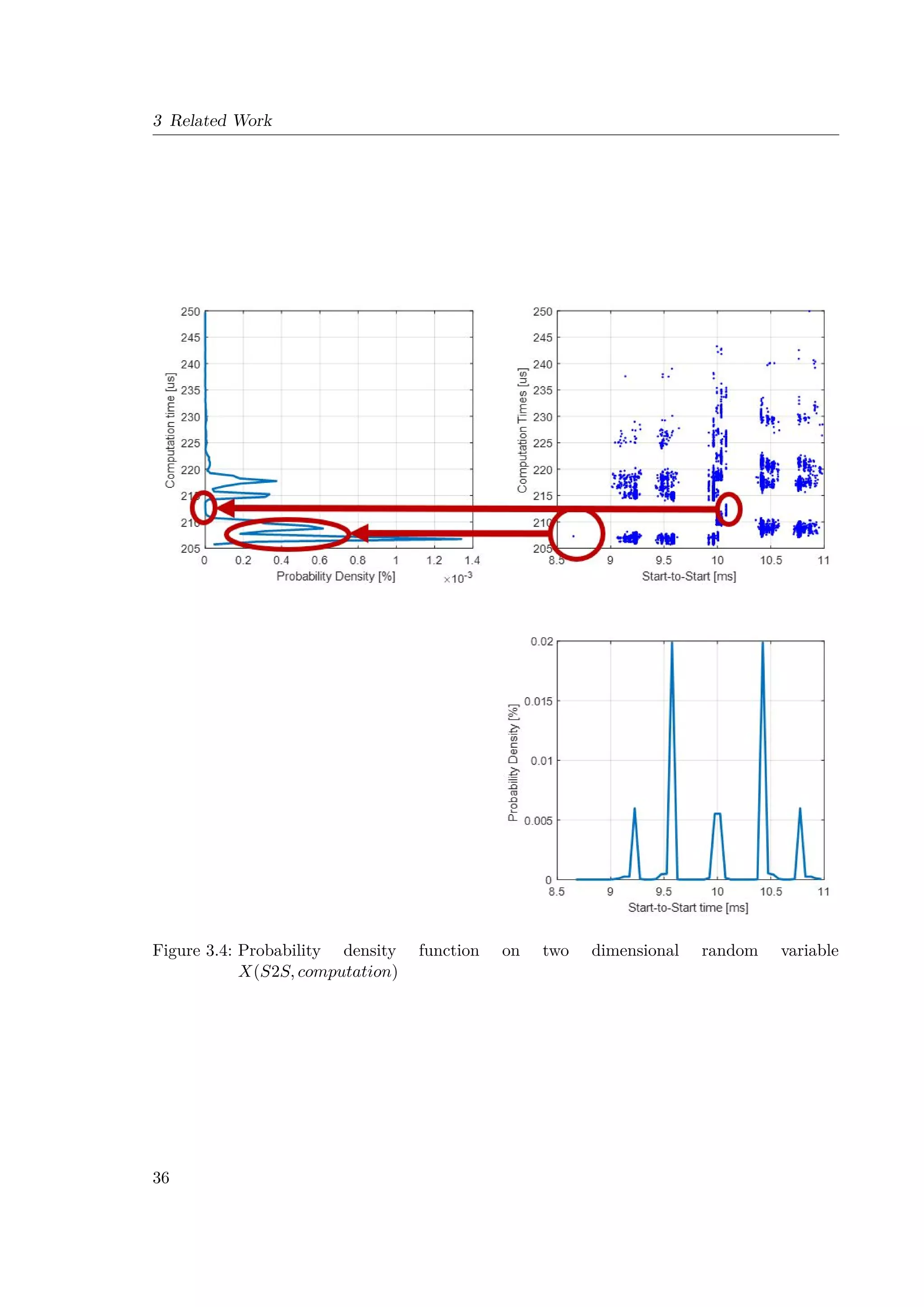
and two dimensional scatter plot is generated, as upper-right plot in Figure 3.4.
Computation time around 212µs falls between two Gaussian distributions in pdf of Com-
putation time and thus according to [9] shall be considered as anomaly. However, taking a
look into the upper-right plot of Figure 3.4, data points with this long computation time,
had S2S time equal to 10.05ms and not falling apart from other data points in 2D space.
Contrary to that, a single data point (lower red round) is far from the rest and thus being an
outlier that could be considered as the anomaly. However, it’s computation time is in range
between 205 − 210µs and by [9] it would be considered as a normal behavior. Due to such
examples, the proposed method [9] resulted in high level of False Alarms that needs to be
reduced in order to be applicable in automotive industry. Hence, the objective of the Thesis
is to increase reduce the number of False Alarms (FPR) while maximizing the Recall. Hence,
the novel Host-based Intrusion Detection method for Real-Time automotive systems, called
AutoSec, is proposed by the Thesis. More about AutoSec will be discussed and explained
in the following Chapters.
35](https://image.slidesharecdn.com/milanthesis-220913145214-138d4713/75/Milan_thesis-pdf-55-2048.jpg)
![4 Concept and Design
Figure 4.1: Typical timing parameters of a Real-Time Task τi - previously explained in Section
2.2.2
Figure 4.2: Example of Execution Diagram using TA Tool Suite [10]
38](https://image.slidesharecdn.com/milanthesis-220913145214-138d4713/75/Milan_thesis-pdf-58-2048.jpg)
![4.1 Timings’ Features
4.1.1 Computation time (Execution time)
First of all, a computation time would be the most reasonable feature as it was already dis-
cussed in Section 3.2.2 - Time-based Anomaly Detection how computation time can be used for
detecting anomalies and what is the overhead of a such approach. However, in this thesis, the
algorithm goes a step further, interconnecting the computation time value with other timing
features. The main reason is that some anomalies cannot be detected using a computation
time only.
Firstly, computation time varies due to many reasons. The main reason is the data size that
needs to be processed. As an example, it is easier to calculate integer values from CAN mes-
sage rather than float values. Furthermore, if in the Runnable function we have some for/while
loops and multiple If statements, this brings further dependencies that influence the compu-
tation time. Since embedded systems, in automotive industry mainly, is highly deterministic,
we can present computation time with one or more combined Gaussian distributions. This
approach was used in [9]. The question raises here: How can we make a hard-line threshold
in here? What happens if the Job/Runnable has been preempted? How these preemptions
influence the computation times due to context switching of the program/code in the CPU?
Due to this, we need other timing features to increase the certainty if something is an anomaly
or not.
The automotive industry is highly demanding industry with high level of standards - Auto-
motive Grade. The main reason is passangers’ safety and security followed by their comfort,
pleasure, leisure and entertainment. Today, we have passed beyond simple transport utility
that moves us from point A to point B. Due to these modern circumstances, automotive grade
sets high standards for technology that passes the bar. Thus, speaking about False Positive
Alarms - we do not want to annoy the driver with warning messages, nor to scare with mes-
sages like Security breach, using our algorithm. The level of False Positives that finds to be
acceptable is 1 False Alarm once a year, recommended once in three years. More about these
values can be read in [26]. Consequently, an objective function to rate the algorithm is to
maximize the True Positive Rate while keeping the False Positive Rate close or equal to zero.
More about these values will be discussed and presented in Chapter 6 - Evaluation.
Before coming to evaluations and testing of the algorithm, other features will be discussed.
The next one talks about the Start-to-Start time.
4.1.2 Start-to-Start
When it comes to S2S time, this feature helps to detect if some other Task / Job / Runnable
was running and pushing the start time of the current one (not necessarily tempered) later in
time. Mainly, this timing is closely related to response time of a Task / Job / Runnable. With
S2S timing feature, we can encapsulate also the knowledge whether a Task / Job / Runnable
skipped its execution when it was planned (scheduled) or even executed more often than it
was supposed to do so.
An example why Start-to-Start time as a feature is very important will be presented through-
out a quick example. In case that an attacker gained an access to the ECU, and the topic of
39](https://image.slidesharecdn.com/milanthesis-220913145214-138d4713/75/Milan_thesis-pdf-59-2048.jpg)

![4.2 Multidimensional Spaces
leading a discussion on evaluations of one feature space dimension(s) over the others, it is
needed to remark the small preprocessing of the data points. The dataset is firstly normalized
and then scaled down by 50% while keeping a center at x = 0.5 and y = 0.5 of the feature
space. Thus, the scaled dataset is now in boundaries [0.25 − 0.75] with the margin around it
as to handle the possibility of new data points exceeding min-max values detected inside the
training data set. Normalization and scale down of points will be used in any case of feature
space combinations.
More about these features spaces, there will be discussion in upcoming subsections: 2D feature
spaces, 3D feature spaces and single 4D feature space.
4.2.1 2D timing feature spaces
Figure 4.3: Example of 2D feature space: S2S vs. Computation time
First feature space that comes under the consideration is 2D feature space. One of the
examples, used in the early stage of the development of the Thesis is depicted in the Figure
4.3. In the figure, the distribution of dataset points in the 2D feature space of S2S vs.
computation time is shown. It can be noticed that data points form groupings that can be
separated as clusters. Coloring is not much of an importance at the this stage of evaluations,
but a quick legend on colors and points will be given.
Different colors present different clusters detected. Points that belong to corresponding cluster
are colored with the same color as the boundary of the cluster. Square black points represent
41](https://image.slidesharecdn.com/milanthesis-220913145214-138d4713/75/Milan_thesis-pdf-61-2048.jpg)


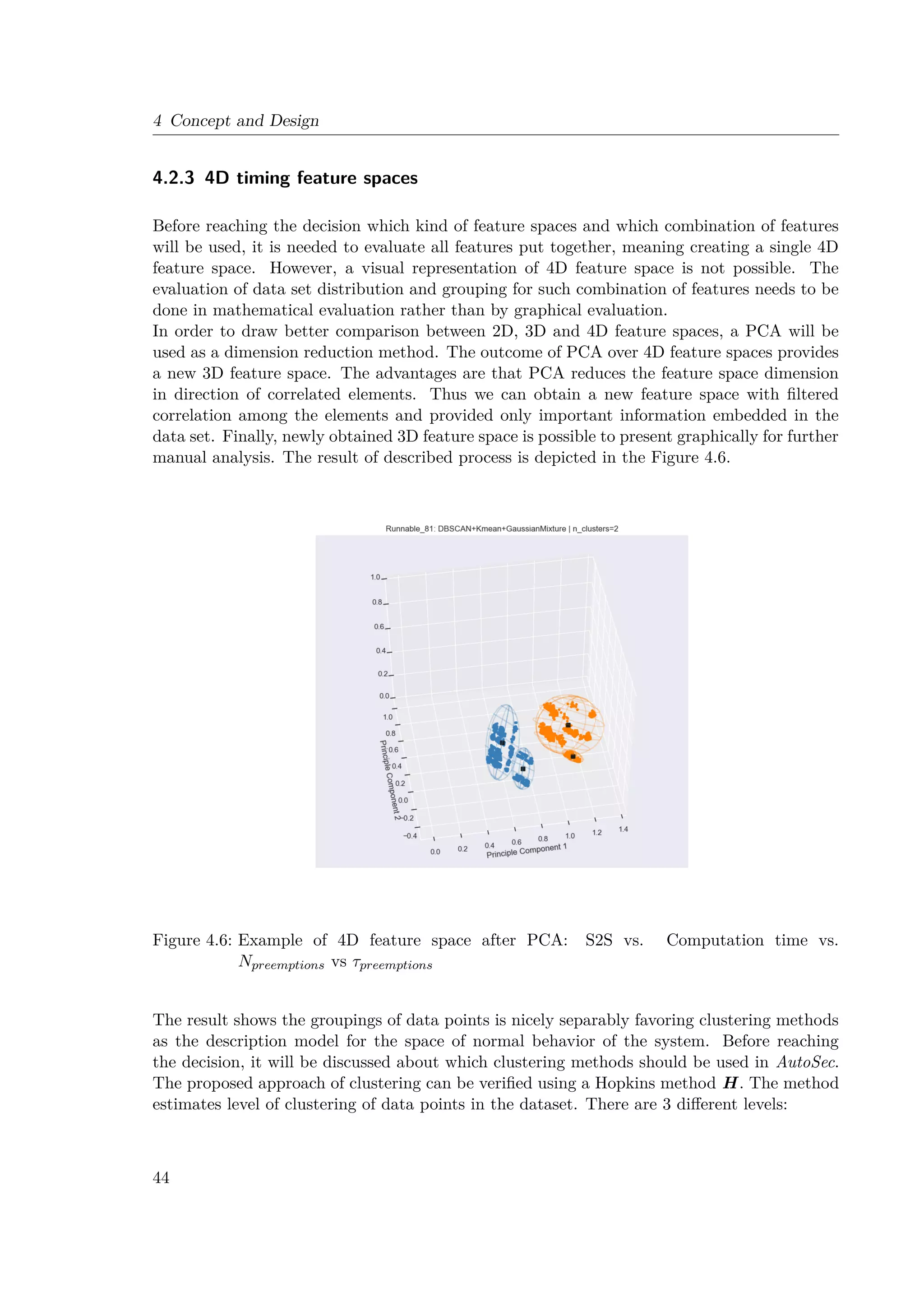


![4.3 Clustering Methods
Figure 4.7: Histogram distribution of two features [Upper-left and bottom-right subfigures]
Computation time needed by Measuring point over time[bottom-left subfigure]
Overlapped distributions of feature 1 and feature 2 with each data point presented
as a square in 2D feature space [upper-right subfigure]
47](https://image.slidesharecdn.com/milanthesis-220913145214-138d4713/75/Milan_thesis-pdf-67-2048.jpg)
![4
Concept
and
Design
Clustering Methods vs. Requirements
R1 R2 R3 R4 R5 R6
Methods
Unsupervised
Learning
Unknown
Number of
Clusters
Unbalanced
Dataset
Non-linearly
Separable
Clusters
Detected Outliers
(training dataset)
Training time
[3183 samples]
K-Mean X X X N.A.
k-Neighbors X X N.A.
Spectral
Clustering
X X X 1.71s
Affinity
Propagation
X X X X 3.12s
Gaussian
Mixture
X X X 0.17s
DBSCAN X X X X X 0.14s
Table 4.1: Requirements evaluation of different clustering methods
48](https://image.slidesharecdn.com/milanthesis-220913145214-138d4713/75/Milan_thesis-pdf-68-2048.jpg)
![4.3 Clustering Methods
In following sections, there will be evaluation and discussion about some clustering methods
with explanation of underlying technique they are using without deeper knowledge and math-
ematical explanations. At the end of this Chapter, a decision, about method to be used, will
be reached, based on features of clustering methods and empirical outcomes they serve for
dataset in the use case of the Thesis.
4.3.2 K-Mean Method
K-Mean clustering method [39] is a method being widely used in dataset with separable data.
As presented previously in Table 4.1, this method requires prior knowledge about the number
of groups in the dataset, meaning the number of separable clusters. Algorithm is based on
iterable process of finding center points of clusters. In each iteration, each point in the data
set will be clustered to the closest center point and being labeled accordingly to the cluster
of belonging. The iterative process stops when the were no changes in labelings between
multiple iterations or if the number of data points below the threshold have been changing
the cluster of belonging repetitively for certain number of iterations in a row. At the end, the
final outcome of clustering will be given.
In a case of K-Mean method, there is a possibility to sort (predict) new points into one of
the clusters detected during a training phase. The function of predict(...), work in the same
as a part of training - it finds the closest center point of them all and then cluster the point
into the cluster with the found center point. Thus, the whole feature space can be mapped
about possible outcomes which data points belong to which cluster. Clusters do not need to
be necessarily clearly separable, as it is depicted in the Figure 4.8. The main downside of this
method in the use case in the Master thesis is that the number of clusters is not known in
advance.
Figure 4.8: Example of K-mean clustering1
However, there are methods that overcome the setback of not having a prior knowledge about
1
source: https://prateekvjoshi.com/2013/06/06/what-is-k-means-clustering/
49](https://image.slidesharecdn.com/milanthesis-220913145214-138d4713/75/Milan_thesis-pdf-69-2048.jpg)
![4 Concept and Design
the correct number of clusters. One of the methods is called Silhouette Method. The Silhou-
ette method is based on K-mean methodology of clustering, by running a K-Mean clustering
on the given set in the range of different number of clusters. The advantage of using Silhouette
Method provides is that the prior knowledge of the correct number of clusters is not needed,
but rather only a range of potential number of clusters.
As an example, the correct number of clusters is in range between 2 and 5. After obtaining
the clustered data points for each case of number of clusters in the given range, an average
distance of points within the same cluster will be calculated. The case of a certain number
of clusters with the minimum average distance of data points within the clusters wins the
arbitration as the most probable correct number of clusters for the given dataset. Thus, the
calculated number of clusters will provide the best clustering results for the tested number
of clusters that could possibly occur in the dataset. After exploiting Silhouette method, the
obtained result can be in further in use the K-mean method. [40]
4.3.3 k-Neighbors
k-Nearest Neighbours (KNN) [41] method can be used for clustering and regression. Since
regression is not in the scope of the Thesis, further discussion about KNN will be related to
clustering only. The core idea behind KNN is to decide on cluster belonging of the examined
point according to belonging of k nearest neighbors. Simplest example is 1-nearest neighbor
- the new point will be sorted into the cluster to which belongs the closest point.
Similarly in case of k nearest neighbors, for k 1, the method searches for closest neighbors.
As the number of k closest neighbors that belong to the same cluster is reached, the new point
will be clustered to the one. However, the value k needs to be chosen carefully, commonly
empirically. The example of such misconception is given in the Figure 4.9. In such case, if
k = 2, the new (green) point will clustered into the cluster with red points. However, in case of
k = 3, the green point will be clustered into the cluster with blue points. By this phenomenon,
initial clustering can oscillate without reaching a steady state during a training phase. Thus
clusters needs a some amount of separation without having overlapping boundaries in between,
what is the case in Figure 4.9.
Figure 4.9: Example of k-Nearest Neighbors clustering2
2
source: https://www.analyticsvidhya.com/blog/2018/03/introduction-k-neighbours-algorithm-clustering/
50](https://image.slidesharecdn.com/milanthesis-220913145214-138d4713/75/Milan_thesis-pdf-70-2048.jpg)
![4.3 Clustering Methods
4.3.4 Spectral Clustering
Spectral Clustering [42] is unsupervised machine learning method that uses unlabeled data.
Theory of graphs is underlying element of Spectral Clustering method. The algorithm used
by this clustering method is to find the most optimal connectivity among data points in
the feature space and upon that to group them into clusters. Eigenvalues and eigenvectors
represent fundamental mathematical tool to construct graphs. The deeper discussion on
mathematical level will not be led here, whilst the algorithm will be used as already built-in
model and function in Python language. More about results of Spectral clustering will be
presented in Section 4.4.
4.3.5 Affinity Propagation
Similarly to Spectral Clustering, Affinity Propagation [43] is unsupervised learning method
that uses also unlabeled data. The method of clustering used by the Affinity Propagation is
based on message passing between data points. Messages sends signals called responsibility
and availability and by these two values, there are availability and responsibility matrices.
Data points that would serve as an exemplar of the cluster will be stored in responsibility
matrix, while other data points will be assigned to availability matrix with the value how
appropriate can the point be assigned to corresponding exemplar. The algorithm is repeated
in iterations until the cluster boundaries are unchanged for specified number of iterations, or
the number of iterations in total reached max number of iterations specified priory to start of
the training, too.
4.3.6 Gaussian Mixture Model
GMM [44] is also one of (semi-)unsupervised clustering methods. The idea behind GMM
is to use data points density to describe them using Gaussian distribution. Thus, Gaussian
Mixture (Model) represents a function consisting of multiple Gaussian distributions. Each
of these k, k ∈ {1, 2, ...K}, distributions used to define Gaussian Mixture Model, represents
a single cluster out of K clusters, how many there are in the dataset. The same problem
here - the number of clusters is priory needed to be known. Similarly, as described in Section
4.3.2.For 1D data set, the Gaussian distribution is described with 2 values: µ - mean value,
and σ - the deviation from mean value. However, if the dataset consists of 2 features, then
the distribution is described using vectors and matrices, since the dataset is in 2D space.
Similarly, for data set in higher dimensions, i.e. n, the distribution is described using a vector
µ (the vector size n×1) and a covariance matrix Σ (the matrix size n×n). Out of covariance
matrix, the eigenvalues and eigenvectors can be calculated. Eigenvectors are used to calculate
the orientation of the distribution in n−D space, while eigenvalues define the deviation from
mean value in each of n dimensions, in local coordinate system anchored to mean value of the
distribution. More about eigenvalues and eigenvectors could be read in [40].
51](https://image.slidesharecdn.com/milanthesis-220913145214-138d4713/75/Milan_thesis-pdf-71-2048.jpg)
![4 Concept and Design
Figure 4.10: Example of k-distance graph with automatically determined value as a first
elbow
4.3.7 DBSCAN
DBSCAN [45] is also one of algorithms that are unsupervised learning without labeled data.
In addition, DBSCAN is immune to outliers in the dataset, and those points will not be sorted
to the closest cluster although they are multiple σ distant from the cluster. The motivation
for DBSCAN is described in the original paper [45] - The application to large spatial databases
rises the following requirements for clusterig algorithms: minimal requirements of domain
knowledge to determine the input parameters, discovery of clusters with arbitrary shape and
good efficiency on large databases.
The algorithm is about simulating human detection of clusters by searching for dense group
of points. Similarly, the DBSCAN algorithm searches points in the neighborhood within
certain range. Firstly, the algorithm chooses random data points as core points, or seeds.
The following step is to examine remaining points if they are in the reach of cores/seeds.
There are 2 different distances used in DBSCAN: direct reachability and indirect reachability.
Direct reachability represents that the examined point is within specified range to the point
of interest (core points - seeds). The DBSCAN algorithm requires one single input parameter,
while there are others that are only optional. The requiring parameter is value representing
the distance for examining reachability. The other (optional) parameter is MinPts - Minimum
Number of Points that needs to be calculated as neighbors within the reachability.
In order to determine the best and MinPts value, there is a simple and effective heuristic
methods that rely on determining those values for the thinnest - least dense cluster in the
dataset. Methods for determining and MinPts are described in [45] (Section 4.2). Only brief
52](https://image.slidesharecdn.com/milanthesis-220913145214-138d4713/75/Milan_thesis-pdf-72-2048.jpg)
![4.4 Clustering Results
overview about determination will be given. The distance d will be calculated as a distance
of a point p to its kth nearest neighbor. For a priory given value k, a function k-distance is
calculated from the dataset to the real number, mapping each point to the distance from its kth
nearest neighbor [45]. The obtain k-dist values are sorted and as such, they create a sorted k-
dist graph. The elbow in the graph represents the most suitable value. However, remarked
in [45], it is very difficult to detect the first valley automatically, but it is relatively simple
for a user to see this valley in a graphical representation. Thus, the interactive and iterable
approach for determining exact threshold point of is needed. The range of value is between
(0, 1]. The example of k-distance graph is presented in Figure 4.10 - k − distances on y-axis,
and sample point in x-axis. More about details on this topic, can be read in [45].
The downside of DBSCAN is not having a possibility of classifying a new point that was not
used during a training phase. The solution to this problem is described in the Section 4.5.
4.4 Clustering Results
Before evaluating different clustering methods on the dataset of timing features related to
the Thesis’s work, the data needs to be normalized and scaled down. Normalization is done
between 0 and 1 - minimum and maximum value in the dataset is found and each point p in
the dataset D is normalized (p-min) / (max-min). Since, we can not be certain that we have
actual possible minimum and maximum value that can occure in the system, the dataset D
will be scaled down to 50% and to keep the center point at 0.5 value. In other words, the
normalization is actually done in range of 0.25 and 0.75 in each dimension of the dataset D.
Throughout this section, different clustering methods described in short in previous section,
will be examined in 2D feature space, i.e. S2S vs. Computation time, and Computation time
vs. Total duration of preemptions (τpreepmtions). In figures to come, different clusters will be
marked in different color, thus it is recommended to read the Thesis in colored version.
First clustering method to be examined is K-Mean. The results for S2S vs. Computation
time and Computation time vs. τpreepmtions is presented in Figure 4.11a and Figure 4.11b,
respectively. The K-mean clustering method outcomes are run on an assumption that the
correct number of clusters in the dataset is priory established. More about this in the following
Chapter 5. As it can bee seen, due to imbalanced density and number of elements per cluster,
K-Mean method does not provide good results. In addition, in Figure 4.11a, it can be seen in
the upper right side of the Figure, a yellow dots are clustered into the yellow cluster although
they are quite distant from the center of the yellow cluster and could be classified as a noise
in the training dataset. Thus, K-Mean does not represent a possible element in the algorithm
of the Thesis.
k-Neighbors - The result for the same combination of features - S2S vs. Computation
time and Computation time vs. τpreemptions are depicted in Figure 4.12a and Figure 4.12b,
respectively. The sensitivity of very close points has a high influence on the algorithm not to
provide quality clustering outputs. Thus, it cannot be used in clustering the features used in
the Thesis.
53](https://image.slidesharecdn.com/milanthesis-220913145214-138d4713/75/Milan_thesis-pdf-73-2048.jpg)
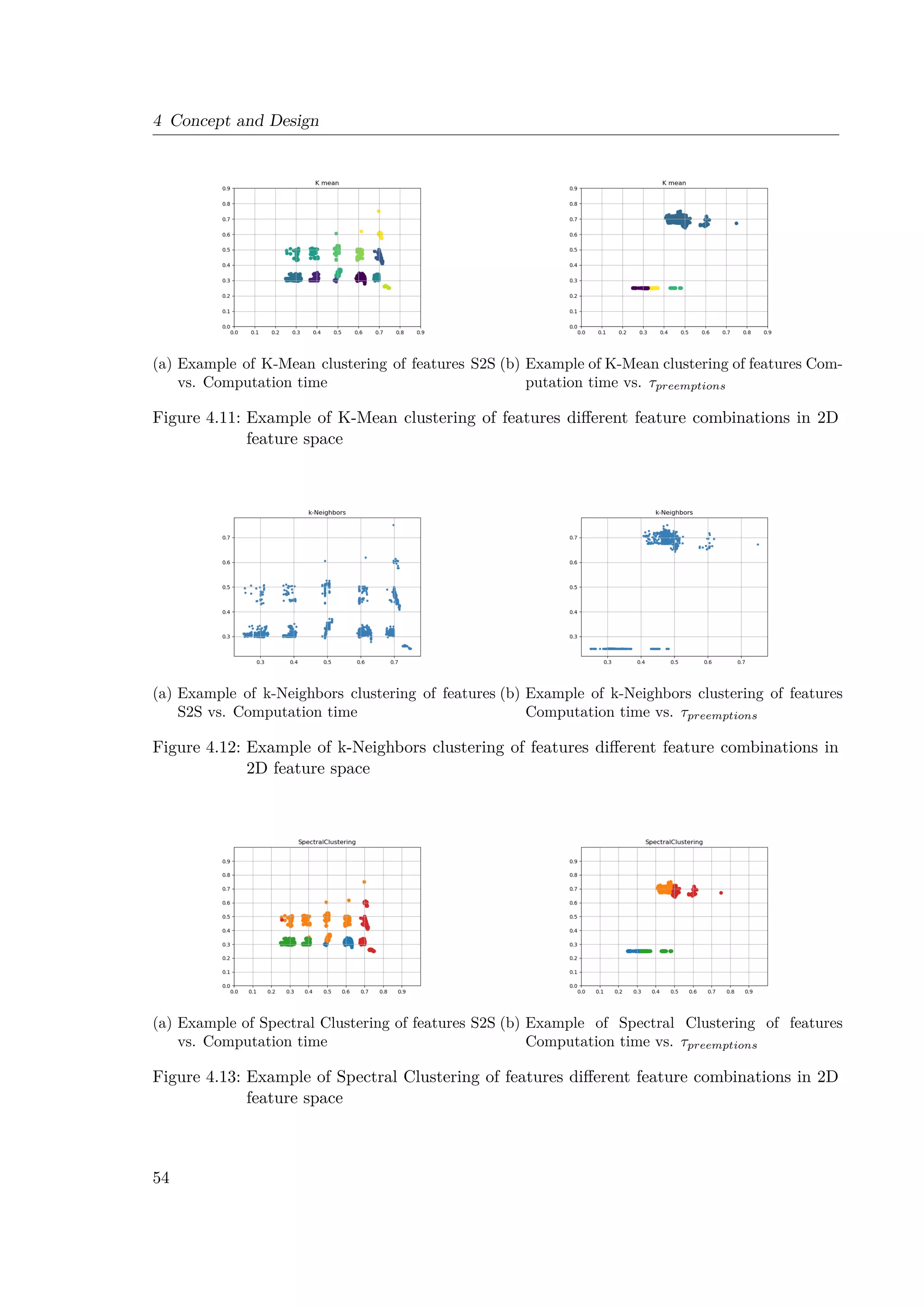

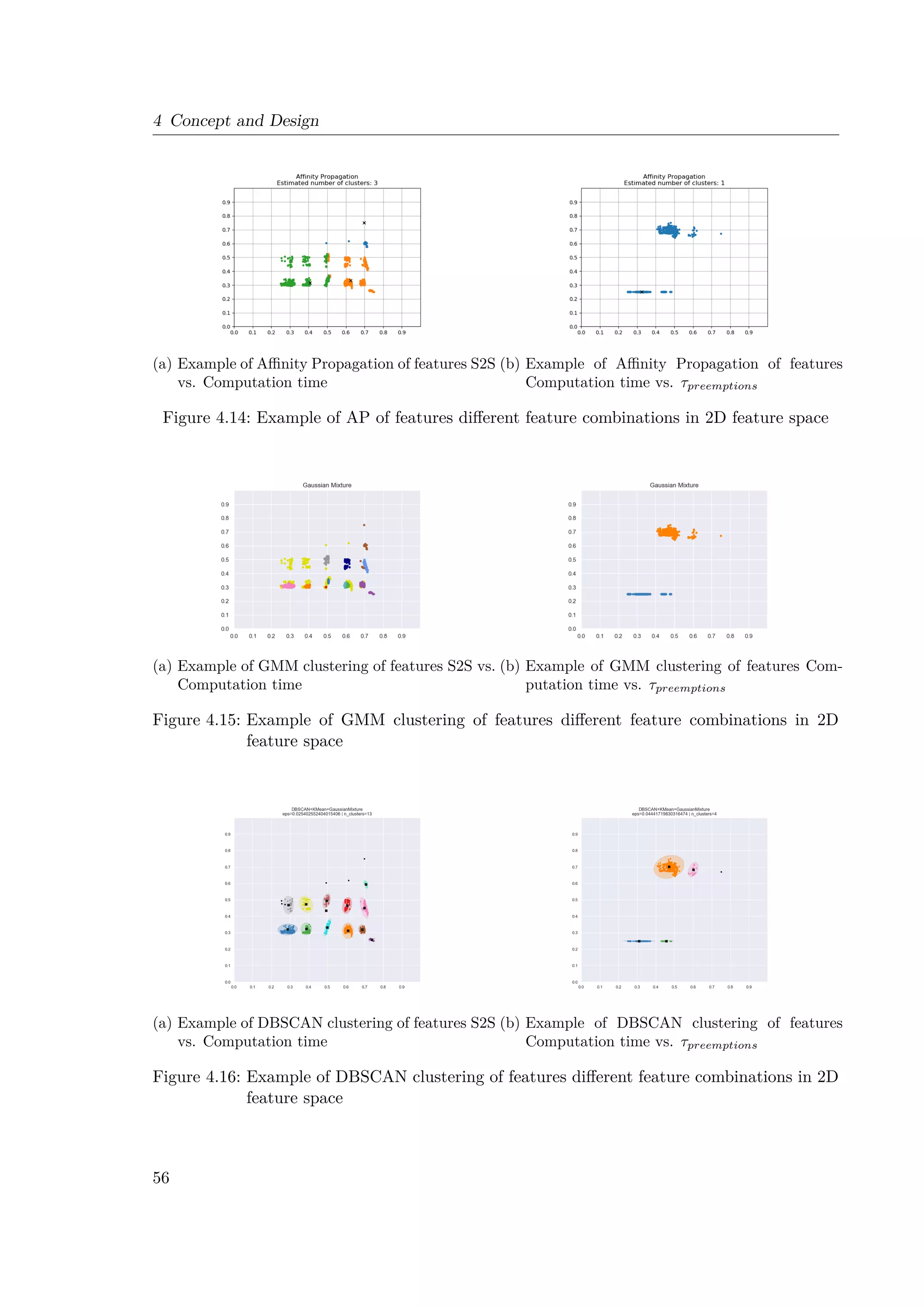
![4.5 How to describe Clusters?
4.5 How to describe Clusters?
Defining algorithms to be used to cluster dataset, next question that is to be answered is
how to use the obtained result so it can be used to predict new data. DBSCAN is a simple
clustering algorithm that provides solution on clustering dataset in whole and not giving an
solution how to cluster new data. Usually, new data will be clustered by DBSCAN using
the whole dataset again. While this is no solution in our case, a new approach needs to
be determined. Throughout this Section, a discussion around the question How to describe
Clusters? will be led.
4.5.1 Number of Clusters
First element as the output of the algorithm is to know how many clusters exist to encapsulate
the dataset elements’ groups. These values are provided by the output of DBSCAN. How-
ever, the correct number of detected clusters can vary widely depending on input parameters
for DBSCAN algorithm. Presented in Section 4.3.7, the main input parameter is value.
Through the literature, there is an algorithm that helps to determine the most appropriate
epsilon for the best clustering results using DBSCAN. The proposed algorithm is k-Distance
measurements [46]. More about it can be read in [45].
The use, only, of the k-Distance algorithm will be evaluated here without examining deeper
meanings of the algorithm. In base line, k-Distance algorithm evaluates distance to n-th clos-
est element in the dataset to the examined data point. This is repeated for m different points
creating the graph depicted in Figure 4.10. As features in the graph, there are multiple stairs,
or elbows. According to [45], the most suitable value is in the elbow position of stairs. The
value is commonly read from the graph, but in the case of this project all of this needs to
be automatized as much as possible since in the real case scenario, there will be hundreds
or thousands of measuring points and for each of them the appropriate value needs to be
determined. Due to that, as part of the Thesis, a script was written to find the elbow in the
system. Depending on the distribution of datapoints in the dataset, due to time constraints
to develop the whole project, the script as elbow finder does not give the prefect result always.
Considering this, the current status of the project provides semi-automatized learning.
During the learning phase, in case that algorithm gives too many clusters on the output with
close grouping of clusters, a conclusion can be pulled that too small has been taken. Thus,
an expert needs to reexamine the case by taking a look into the k-Distance graph an manu-
ally read the correct value and finally rerunning the training process with manually chosen
value. With the elbow finder script, training time is reduced, but the training phase at the
current stage needs to be taken with precautions to reevaluate the outputs manually in order
to rerun training for certain measuring points with poorly chosen value.
At the end, evaluating that all have been chosen to minimize number of clusters and mini-
mize the sparsity of data points inside each cluster, we reach the point to determine how to
describe obtained clusters using DBSCAN for later Online/Offline use. More about this is
given in the upcoming Section.
57](https://image.slidesharecdn.com/milanthesis-220913145214-138d4713/75/Milan_thesis-pdf-77-2048.jpg)


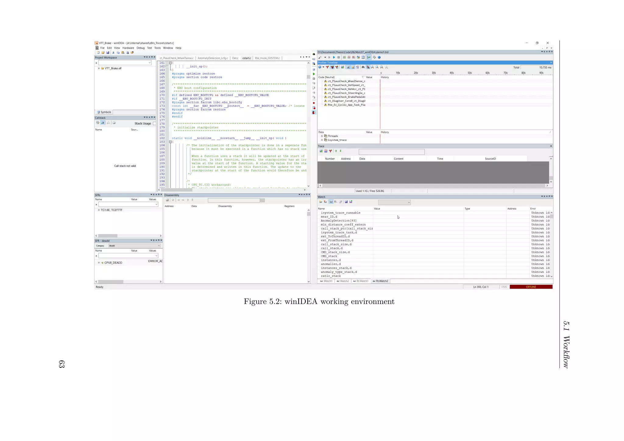
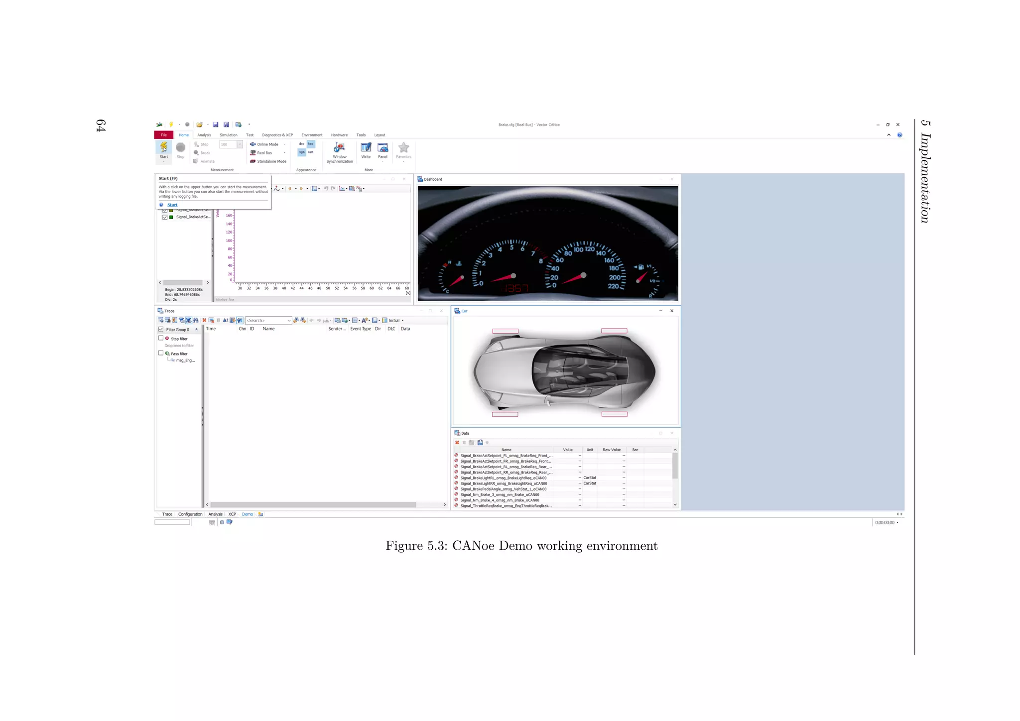

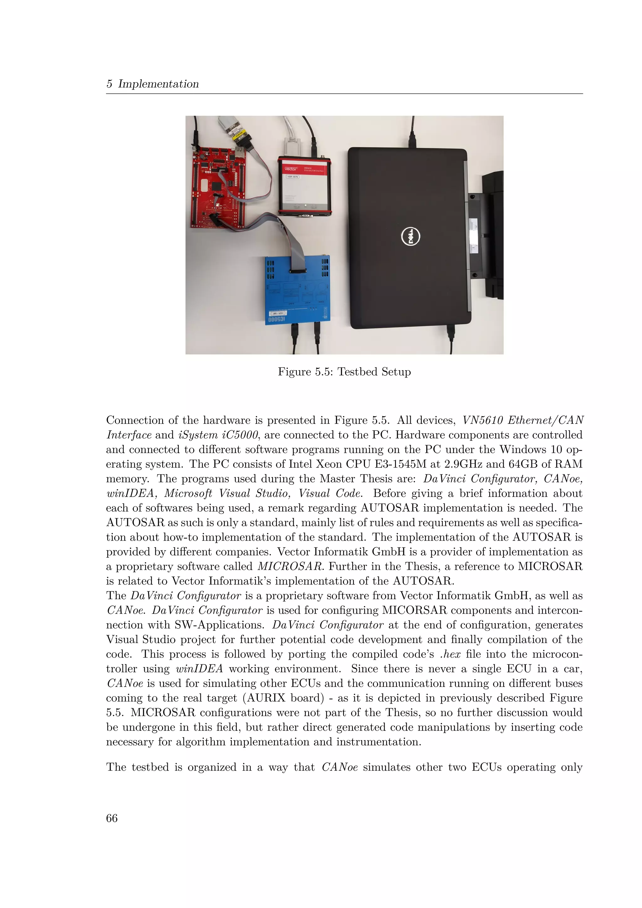

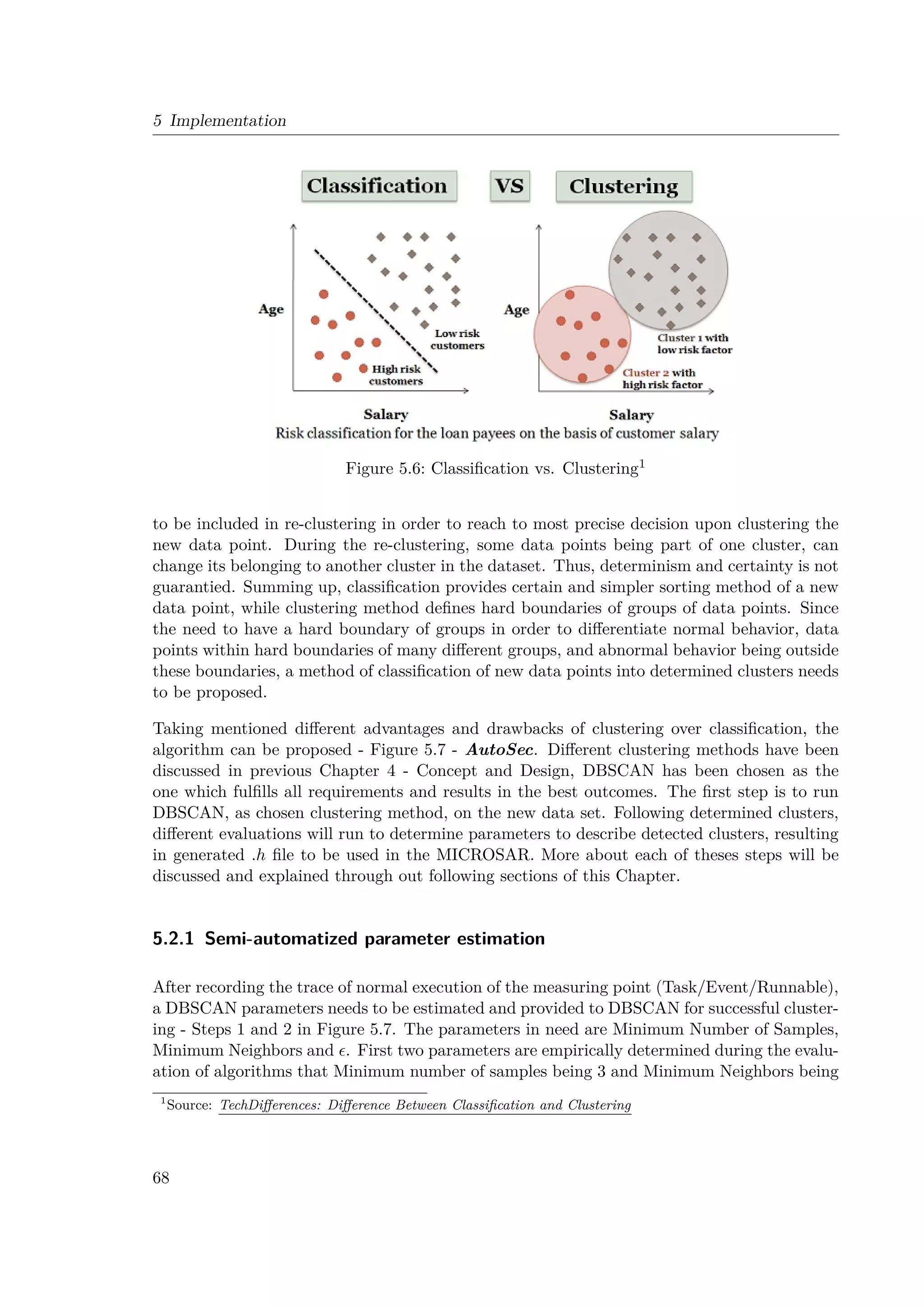

![5 Implementation
Figure 5.8: k-Distance graph calculated on one of the measuring points from the Thesis
first elbow in the k-Distance graph represents the suitable value to be used for DBSCAN.
More about and DBSCAN can be read in [45].
Unfortunately, dependent on the data set itself, value of the first elbow might produce
too many clusters (Figure 5.9), and some part of them are in a close proximity, while the
others are quite distance forming another dense group of clusters. The conclusion reaches
the point that those clusters in close proximity would need to be merged and thus forming
smaller number of clusters in more intuitive way. The example is given comparing Figure
5.9 and Figure 5.10, using lower and higher values, respectively. The downside of the
estimation step in AutoSec algorithm, is the external expertise is needed to evaluate chosen
value. Thus, this step is called Semi-automatized parameter estimation, since the will
be chosen to the best capabilities of k-Distance method and in that way minimize the time
to estimate thousands of values for thousands of different measuring points in the System.
However, external expertise is needed to validate and verify the automatically chosen value
whether it produces clustering outcome with as good as possible trade-off between: distance
between clusters, size of clusters and number of clusters. This part can be called Validation
phase, corresponding to the standard Validation phase in Machine Learning pipeline. The
main difference is that, best to author’s knowledge, no automatic method exists to validate
chosen with constraints of trade-off between: distance between clusters, size of clusters and
number of clusters. The drawback of AutoSec, in some specific cases, an would need to be
manually chosen with the higher value reading it from the second, third, or later elbow in the
k-Distance graph.
70](https://image.slidesharecdn.com/milanthesis-220913145214-138d4713/75/Milan_thesis-pdf-90-2048.jpg)


![5.2 Training
5.2.3 Optimal Number of (Sub-)Clusters and their measures
After detecting clusters in the data set and mapping data points to its corresponding cluster,
as well as disregarding outliers present in the training data set, next step is to describe clusters
by its middle point and size, as described in Section 4.5 - Step 4 in Figure 5.7.
Examining Figure 5.11, especially taking blue and red clusters into the consideration, it can
be seen in the given Figure, that each cluster is described using two boundaries embodying
its data points. The explanation will be given on the blue cluster. Taking a closer look on
it, data points forming blue cluster are two groups that can be considered as two subclusters.
The reason behind these two subclusters are not recognized as two different clusters is due to
the data points between them forming a bridge between them and thus connected these two
(sub)clusters. Thus, these two subclusters form a single bigger blue cluster, in comparison
to brown and green cluster that are highly close, but no bridging data points in between to
connect them.
At this point, there is a reasoning why two boundaries have been used to describe the blue
cluster instead of single one. The reason is: blue cluster is formed out of two subclusters that
each of them can be described with different Gaussian distribution function. Thus, the blue
cluster can be described as mixture of combined different Gaussian distribution functions.
Using the approach describing big clusters as mixture of different Gaussian distribution func-
tions, gives the freedom to describe any shape and form of cluster that is not necessarily
rounded in thus to be described with only a single Guassian distribution function. The prob-
lem aroused when, AutoSec reached the point to describe such clusters as the blue cluster in
the following Figure 5.12. Such cluster needs to be described using multiple different Gaussian
distribution function. The following part will be executed n times (n loops) corresponding
that n different clusters are found in the data set.
In order to do so, the Silhouette Method is used to estimate how many subclusters the big
cluster has, if any (Best result 70%)2 - Step 5 in Figure 5.7. The meaning is how many
Gaussian distributions are needed in order to describe the big cluster. The Silhouette Method
runs K-Mean method with many different values for K (number of clusters) only on the data
points belonging to the big cluster, i.e. blue cluster in the case of Figure 5.12. The Silhouette
method will iterate K-Mean clustering over K being in range [2, 4]. These values needs to be
predefined in a case of the algorithm, depending on how many subclusters could be detected
in a single cluster. If number of subclusters is to big, the overfitting can be reached and
overloading final outcome of AutoSec. Thus, a reasonable number of subclusters needs to be
defined. The measure to determine the number of subclusters used by Silhouette Method is
how close each point in one cluster is to points in the neighboring clusters. The visual results
of the outcome is presented in Figure 5.13. If Silhouette Method outcome, for any value of K
in the predefined range of potential number of subcluster, surpasses the predefined threshold
of 70% (Hopkins value), the corresponding value of K will be taken into the further use.
If K has been determined as the result of a big cluster having subclusters, a K-Mean clustering
for the calculated K-value will be taken - Step 6 in Figure 5.7. Following the algorithm
2
70% (0.7) is taken as a threshold based on the Hopkins value as the level of highly separable clusters
3
Source code used for running Silhouette Method: scikit Learn: Silhouette Method
73](https://image.slidesharecdn.com/milanthesis-220913145214-138d4713/75/Milan_thesis-pdf-93-2048.jpg)


![5.4 Online System
implementation, this measuring points used by the debugger for tracing are maintained also
during an online implementation of the algorithm. The debugger timing readings are main-
tained for debugging and verification of the online algorithm implementation and calculations.
Since the debugger timings cannot be used in the online calculations, the local MCU clock is
used to measure online timings. The structure of timings is presented by pseudo-code Algo-
rithm 1. The debugger reads new entity being ran using the variable isystem_measuringPoint.
When the debugger, as mentioned, detects the value change in the variable, it reads its own
local time as the timestamp. Contrary to that, the online algorithm reads the time from
the MCU timestamp = GetMCUTime(). The function GetMCUTime reads the internal
clock value of the MCU. The clock value is determined using counter that is reset when it
reaches maximum value and then starts counting from 0 again. Thus, new offset needs to be
set whenever the counter is reseted. The offset is incremented everytime this happens. The
incrementation of the offset has the value of the maximum counter value.
Following reading time on the MCU, the debugger will be notified about context change
through out the variable isystem_measuringPoint. Only afterwards, the measuring points
will be notified about the context change using the previously recorded time. The order of
execution is due to minimizing time indifference between time read by MCU and time when
the debugger has been notified. However, very important remark follows.
By the end of the Master Thesis, it is noticed that time read by MCU and by the debugger
tend to have certain indifference that is not constant. This indifference will be explained later
in conclusion for the further work. Many different reasons might be the cause of a behavior.
Potential cause is the overhead in the debugger, by debugger: accessing and reading the vari-
able, reading its local time, processing the data, etc.
Regarding the other functions start, finish, preempt, continue, a brief overview will be given.
Each measuring point is created as an structure consisting of following elements:
• StartTimes[2] (array of floats);
• StartToStart (float);
• computationTime (float);
• numberOfPreemptions (int);
• durationOfPreemptions (float);
• checkpoint (float);
When start(...) function is called, a measuring point inserts the timestamp value in the array
of StartTimes. The first value in the StartTime array is a start time of the previous instance,
while the second value in the array corresponds to the start time of the currently running
instance of the measuring point. The StartToStart value is calculated as the difference be-
tween these two values: StartToStart = StartTimes[1] − StartTimes[0]. Other values of
computation time, number of preemptions and duration of preemptions have been reset to
0 value. The checkpoint value is initialized to the timestamp value. Checkpoint is used for
calculating mid-calculation values when a measuring point is preempted, as it is explained
79](https://image.slidesharecdn.com/milanthesis-220913145214-138d4713/75/Milan_thesis-pdf-99-2048.jpg)

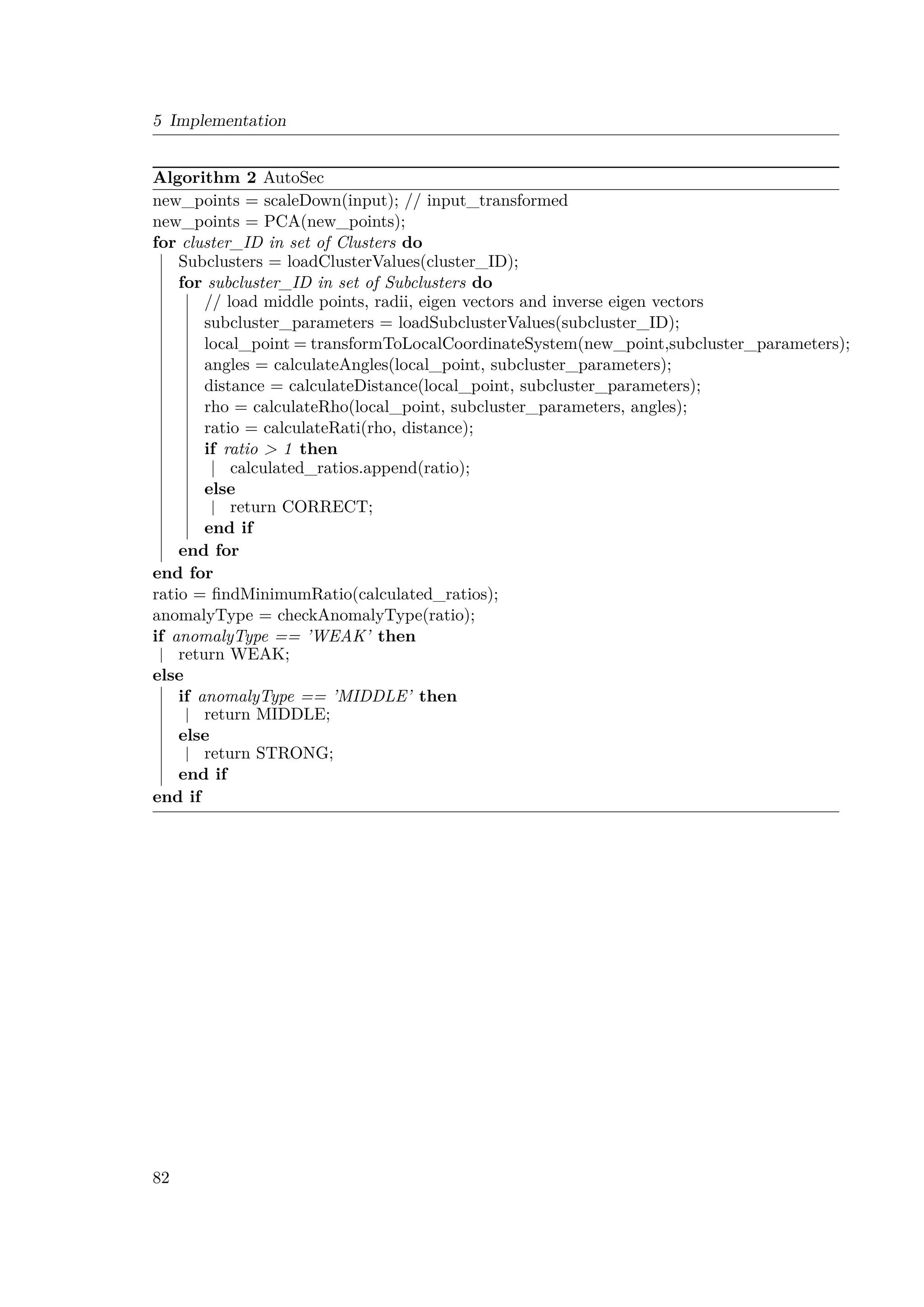
![Chapter 6
Performance Evaluation
The evaluation of an algorithm or a method depends on what is the target of research and
goal to be achieved. Basic requirements are related to the hardware architecture for which
the algorithm is developed. Thus, requirements related to the working environment are:
• calculation time in range of tenths of microseconds - due to high number of potential
measuring points (more than ten thousands in some cases)
• low overhead - due to program execution on the MCU
In addition to that, there are qualitative requirements commonly used in an evaluation of
Machine Learning algorithms. Thus, the main requirements for a problem stated by the
Thesis are:
• Low False Positive Rate - reference value 1e − 4 by [9]
• High Recall - reference values 75% for HIDS by [9], or 81% for NIDS by [26]
• High Precision
The meaning of False Positive, Recall and Precision, and other measures used for Machine
Learning algorithm evaluation, will be explained in the following Section 6.1.
6.1 Evaluation Parameters
In order to evaluate the outcomes of Classification method, such as the outcome of AutoSec,
a confusion matrix is commonly used. The confusion matrix represents a matrix n × n,
representing a cross section of classification results, as depicted in the Figure 6.1. On the
diagonal it is represented how many elements are classified correctly, i.e. element of a class
type A has been successfully classified in 85% as a type A. However, it was misplaced in 15%
of cases, out which it was misplaced with type B in 10% and 5% misplaced by type C.
In case of ours, there are two types of classes - Normal and Anomaly. Thus, the confusion
matrix has a size 2 × 2. The confusion matrix in case of outliers/anomalies detection is given
in Figure 6.2. In case of confusion matrix for outliers/anomalies, fields have specific naming,
83](https://image.slidesharecdn.com/milanthesis-220913145214-138d4713/75/Milan_thesis-pdf-103-2048.jpg)
![6 Performance Evaluation
Figure 6.1: Example of a Confusion Matrix
Figure 6.2: Confusion Matrix for Outlier/Anomaly Detection
as follows:
• True Negative (TN) - Normal is detected successfully
• True Positive (TP) - Anomaly is detected successfully
• False Positive (FP) - Anomaly is NOT detected; known as Type Error I
• False Negative (FN) - Normal is detected as Anomaly; known as Type Error II
Depending on the application for which the method is developed, ones tend to minimize False
Positives (False Alarms), others tend to minimize False Negatives. In the case of HIDS, the
requirement stated that False Positives needs to be minimized, while achieving reasonable
True Positive value (i.e. higher than 50%). The reasoning behind the requirement is not
to warn the driver with potential security breaches unless the system is highly certain that
the breach took place. The outcome will be seemingly lower level of True Positives and thus
higher level of False Negatives, meaning that quite number of anomalies will pass the system
undetected. Although, some anomalistic behavior can be passed undetected, still there are
others that would trigger the alarm. In automotive industry, the important element is not to
overflow a driver with the information unless it can be with high certainty classified as highly
important and relevant information to be delivered to the driver. However, apart from Type
Error I and II (False Positive and False Negative, respectively), there are other additional
measures to evaluate the outlier detection algorithm.
When it comes to the evaluation of detecting outliers, as anomalies in the case of AutoSec, it is
not often an easy task. The reason is described in-depth by [40]. The drawback in detecting
84](https://image.slidesharecdn.com/milanthesis-220913145214-138d4713/75/Milan_thesis-pdf-104-2048.jpg)
![6.1 Evaluation Parameters
outliers, or anomalies, and evaluating an algorithm to detect so, is lack of ground-truth,
meaning no labels of outliers and anomalies are available. Following paragraph is quoted
from [40]:
In outlier detection, a more reasonable (albeit imperfect) approach is to use external validity
measures. In some cases, the data sets may be adapted from imbalanced classification problems,
and the rare labels may be used as surrogates for the ground-truth outliers. In such cases, a
natural question arises as to how the ground-truth can be used to evaluate effectiveness. Most
outlier-detection algorithms output an outlier score, and a threshold on this score is used to
convert the scores into outlier labels. If the threshold is selected too restrictively to minimize the
number of declared outliers, then the algorithm will miss true outlier points (false negatives).
On the other hand, if the algorithm declares too many data points as outliers, then it will lead
to too many false positives. This trade-off can be measured in terms of precision and recall,
which are commonly used for measuring the effectiveness of set-based retrieval.
Precision is defined by Eq. 6.1. The Precision gives the result of how many true anomalies
have been detected out of all reported cases. An example for Precision = 95% means that
out of 100 reported cases (outliers), 95 of them are true anomalies, whilst other 5 cases are
normal behaviors reported as outliers.
Precision =
TP
TP + FP
(6.1)
Recall is defined by Eq. 6.2. The result of Recall shows the capability of an examined
method, i.e. how many anomalies out of all known anomalies have been successfully detected.
Thus, the Recall = 80% means that 80/100 anomalies are detected, the other 20 anomalies
passed undetected, below the set threshold. The other name for Recall is also True Positive
Rate (TPR).
Recall =
TP
TP + FN
(6.2)
FPR, defined by Eq. 6.3, is, contrary to TPR, a ratio how many instances of normal behaviors
surpassed the threshold and have been reported as outliers.
FPR =
FP
FP + TN
(6.3)
By defining these values, outcomes of those will be used to evaluate the achievement of AutoSec
and fulfilment of set requirements. The algorithms to be used head-to-head are AutoSec and
[9] used as HIDS. In the paper [9], the tests were run on two different threshold levels - lower
and higher sensitivity level. The achievements presented in [9] were:
• FPR
FPRlower = 0.6897%
85](https://image.slidesharecdn.com/milanthesis-220913145214-138d4713/75/Milan_thesis-pdf-105-2048.jpg)
![6 Performance Evaluation
FPRhigher = 0.098%
• Precision
Precisionlower = 98.54%
Precisionhigher = 99.89%
• Recall
Recalllower = 88.43%
Recallhigher = 45.12%
Since the paper implemented their proposed algorithm (SecureCore) onto different hardware
architecture, the specific implementation of the same algorithm in AUTOSAR due to time
limitation was not directly implemented. The results presented in the paper [40] are used as
such as a trend setter.
6.2 False Positive Rate (FPR)
First evaluation step is to evaluate how many false alarms, algorithm tends to report. By
doing this, the threshold is set to satisfy requirements. Since the requirements in case of the
Thesis is to minimize the FPR, threshold will be set higher by reducing the Recall. Trade
off of this can be discussed upon Figure 5.15 from the previous Chapter 5 - Section 5.3. In
the Figure can be observed that threshold for ratio value shall be placed between value 2 and
3. Thus, the fuzzy anomaly level should be used, as discussed in Chapter 5 - Section 5.3:
WEAK, MEDIUM and STRONG anomaly. Thus, for simplicity reasons a hard threshold
was taken for all measuring points. The threshold values depends highly on the measuring
points, i.e. in the Figure 5.15 a value 2 could be taken as a threshold, whilst for some other
measuring point it could be value 3. In order to avoid this dependencies, and to have a hard
threshold as used in [40], a single threshold value will be used: threshold = 2.5. By doing
this, a results would be than rather pessimistic and it will downgrade the Precision and
Recall results. Therefore, the important remark announces that for real-world applications
in industrial production shall take evaluation on each measuring points and set thresholds
accordingly.
The Thesis has run the evaluation with fixed threshold of 2.5 for measuring point on the
Runnable Level and on the Event Level corresponding to higher and lower sensitivity levels,
similarly to sensitivity levels evaluated in [40]. The evaluation is run on the program allegedly
without any anomalies present in it. In later evaluation of IDS, FPR will be reevaluated under
circumstances that there were actual anomalies being injected.
Since some Runnables are triggered upon received data through CAN communication, this
can shift the order of execution of other Runnables. In order to include such elements into
the evaluation of FPR, the program will start with the execution and later in time, CAN
communication will start sending data: i.e. there will be no CAN communication and it will
86](https://image.slidesharecdn.com/milanthesis-220913145214-138d4713/75/Milan_thesis-pdf-106-2048.jpg)

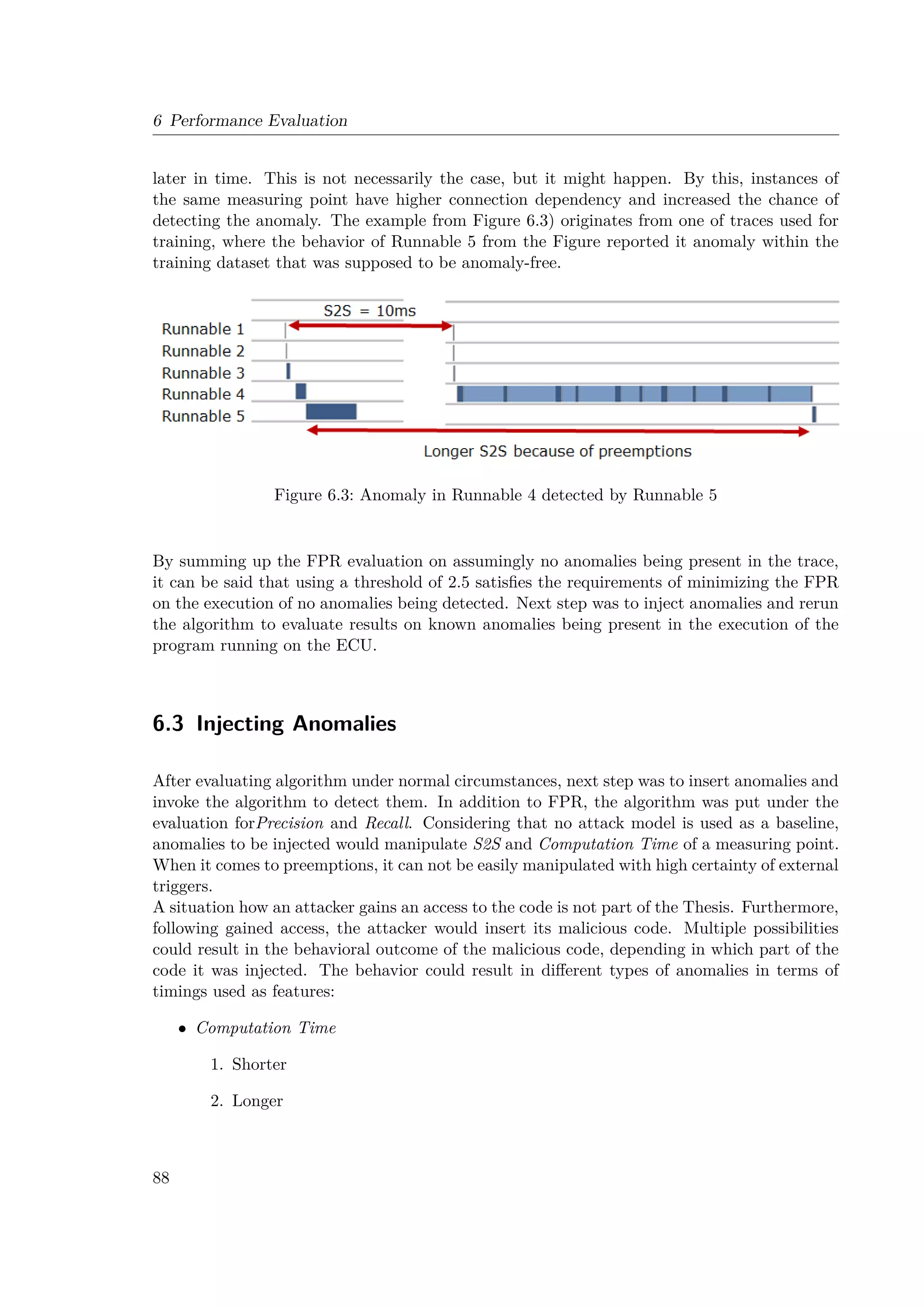
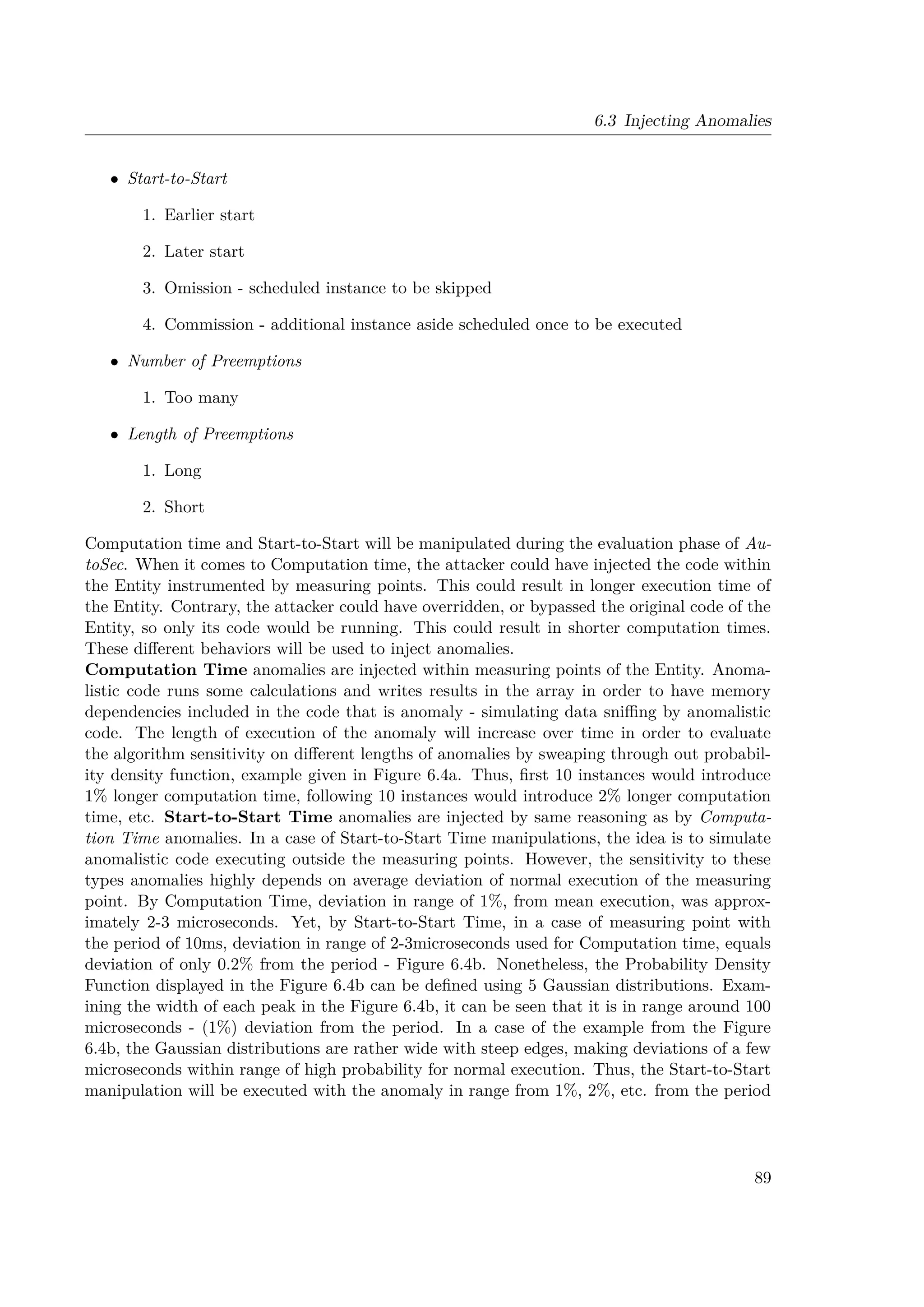

![6.4 Results
Runnable Level Event Level
S2S Time
Anomaly
[1..25%]
deviation
[25..40%]
deviation
[1..20%]
deviation
[25..40%]
deviation
FPR 0.00605632% 0.02004812% 0.01976089% 0.01978351%
Recall 33% 79% 34% 64.52268361%
Precision 99% 98.77% 97.18% 98.46047794%
Table 6.1: Results on FPR, Recall and Precision for Start-to-Start-time type of injected
anomalies
industry - FPR should have been below 1e − 19 that is super extreme value. Thus, additional
evaluation shall be included for evaluating reported anomalies based on additional external
information that require high overhead in implementation.
Before giving the comparison between obtained result by AutoSec and results of the Se-
cureCore from [40], Computation Time will be evaluated. The results of Computation time
anomaly injections are presented in Table 6.2. Values are average values over 5 different test
cases for Runnable level and 4 different test cases for Event level.
As presented through the Thesis, Runnable level is fine-granule level that is more sensitive
to deviation and anomalies in behavior. The results of the evaluation shows that: in case
of 5-10% deviation resulted in Recallcomputation = 100% for Computation anomalies and
RecallS2S = 79% for S2S anomalies. It is important to say that, in most cases based on
deviations on each feature, a hard threshold could be defined, i.e. if Computation time longer
than x or shorter than y value, reported as an anomaly. These values of obvious anomalies
beyond easily determined hard threshold were not taken into the consideration, but rather
values that are within these boundaries. The best representation is depicted in the Figure
6.5a.
In Figure 6.5a, the change of features’ values over time is displayed. By mark dots, anomalistic
instances are marked. In Figure 6.5a, on x − axis of each feature is the instance ID equal to
timeline. On y − axis of each graph is the value corresponding to the feature.
As it can be seen in Figure 6.5a, anomalies (red points) are in between hard thresholds. In
case of S2S, hard thresholds would be longer than 11.5ms and shorter than 8.5ms. By taking
a closer look by zooming, the better look is displayed in Figure 6.5b. As it can be seen,
instance having an S2S of exactly 10ms value in combination with other features is reported
as the anomaly since it does not fit in the normal execution. Anomalies were detected since
91](https://image.slidesharecdn.com/milanthesis-220913145214-138d4713/75/Milan_thesis-pdf-111-2048.jpg)
![6 Performance Evaluation
(a) Anomalistic instances (marked by red) on each feature over time of traced measuring point
(b) Features over time of traced measuring point [zoomed Figure 6.5a]
Figure 6.5: Anomalistic instances (marked by red) on each feature over time of traced mea-
suring point
92](https://image.slidesharecdn.com/milanthesis-220913145214-138d4713/75/Milan_thesis-pdf-112-2048.jpg)
![6.4 Results
Runnable Level Event Level
Computation
Time
Anomaly
[1..10%]
deviation
[5..15%]
deviation
[1..10%]
deviation
[5..15%]
deviation
FPR 0.030305% 0.015% 0.00499% 0.010068%
Recall 76.5% 100% 22% 56.5%
Precision 98.115% 99.26% 98.81% 99.09%
Table 6.2: Results on FPR, Recall and Precision for Computation-time type of injected
anomalies
they have been too far from the closest cluster. The result is depicted in Figure 6.6, whereas
the axis are now Principle Component 1 vs. Principle Component 2 vs. Principle Component
3 - new feature spaces in 3D space obtained from original 4D timing feature space by PCA.
Detected anomalies are presented by black dots, and different cluster with different cluster
whose middle point is depicted by black square point. Due to limitation of presenting 3D
space as a figure of 2D dimensions, some anomalies seems to be within the cluster, however
if we would be able to rotate the picture, it would be seen that it does not belong to any of
clusters.
Another interesting example, why combination of different timing features is important is
present in Figure 6.7. Taking a look into the exact values of reported anomalies, it can be
seen that values for S2S feature are among normal execution. The computation time is in
range of occasional longer computation times that are around 110 microseconds. Number of
preemptions in cases of anomalies is is None and thus the duration of preemptions is equal to
zero. Examining each of those features separately shows nothing uncommon or non-ordinary.
Nonetheless, overlapping these features, a reason reveals that longer computations in range
around 110 microseconds happen in some cases if only a preemption has happened. Since, in
the case of anomalies for that long computation time, no preemptions happened, algorithm
has detected those instances as an anomalisitc instances.
Results presented in the Table 6.2 and Table 6.1 are average values of all tests that were
rather pessimistic and strict on evaluation of AutoSec method. Tests were designed in a way
that anomaly values are in the range of high probability of timing features. By this approach,
it was tested how good AutoSec can detect anomalies that appear common by each separate
timing, while being an outlier and anomaly when all timing features are combined.
93](https://image.slidesharecdn.com/milanthesis-220913145214-138d4713/75/Milan_thesis-pdf-113-2048.jpg)


![6 Performance Evaluation
Figure 6.8: FPR vs. Recall - Runnable level vs. Event Level
Tests were designed to test this type of anomalies, whilst the values beyond some hard thresh-
olds could be with high Recall and low FPR detected by using simple threshold values based
on examining Probability Density Function by experts. In following Figures are presented
scatter plots of run tests with different time deviation. The conclusion can be drawn on
difference of different tracing resolution: Runnable Level vs. Event Level (Figure 6.8). The
results on Event Level have lower Recall in comparison to Runnable Level, due to coarse reso-
lution of timings and thus small deviation in a few microseconds within one Runnable traced
under the Event could not have been detected as it would be the case if that Runnable was
monitored independently and separately. By similar reasoning, if one Runnable is traced, it is
more sensitive to computation timings of its own than by deviation of timings from previous
Runnable. If previous Runnable has some longer execution time, it should have some higher
degree of deviation in order to influence significantly S2S parameter of Runnable under mon-
itoring. The reasoning is behind different magnitude of timings in Computation times and
Start-to-Start times since 1% out of 10ms and 1% of 200µs are 100µs and 2µs, respectively.
Therefore the results of Tests on Start-to-Start Anomalies have lower Recall then Compu-
tation Anomalies test results, in both cases of Runnabble Level (Figure 6.9) or Event level
(Figure 6.10) of monitoring.
Papers listed in Chapter 3 do not list their results under same evaluation values. Some pa-
pers have only discussed the results, without providing the exact numbers, while others have
evaluated their method using acFPR and Recall, or Recall and Precision, or only one of
these 3 parameters. Figure 6.11 demonstrates a comparison between AutoSec and following
IDS methods - [cite papers here], which used FPR and Recall as evaluation values. In addi-
96](https://image.slidesharecdn.com/milanthesis-220913145214-138d4713/75/Milan_thesis-pdf-116-2048.jpg)

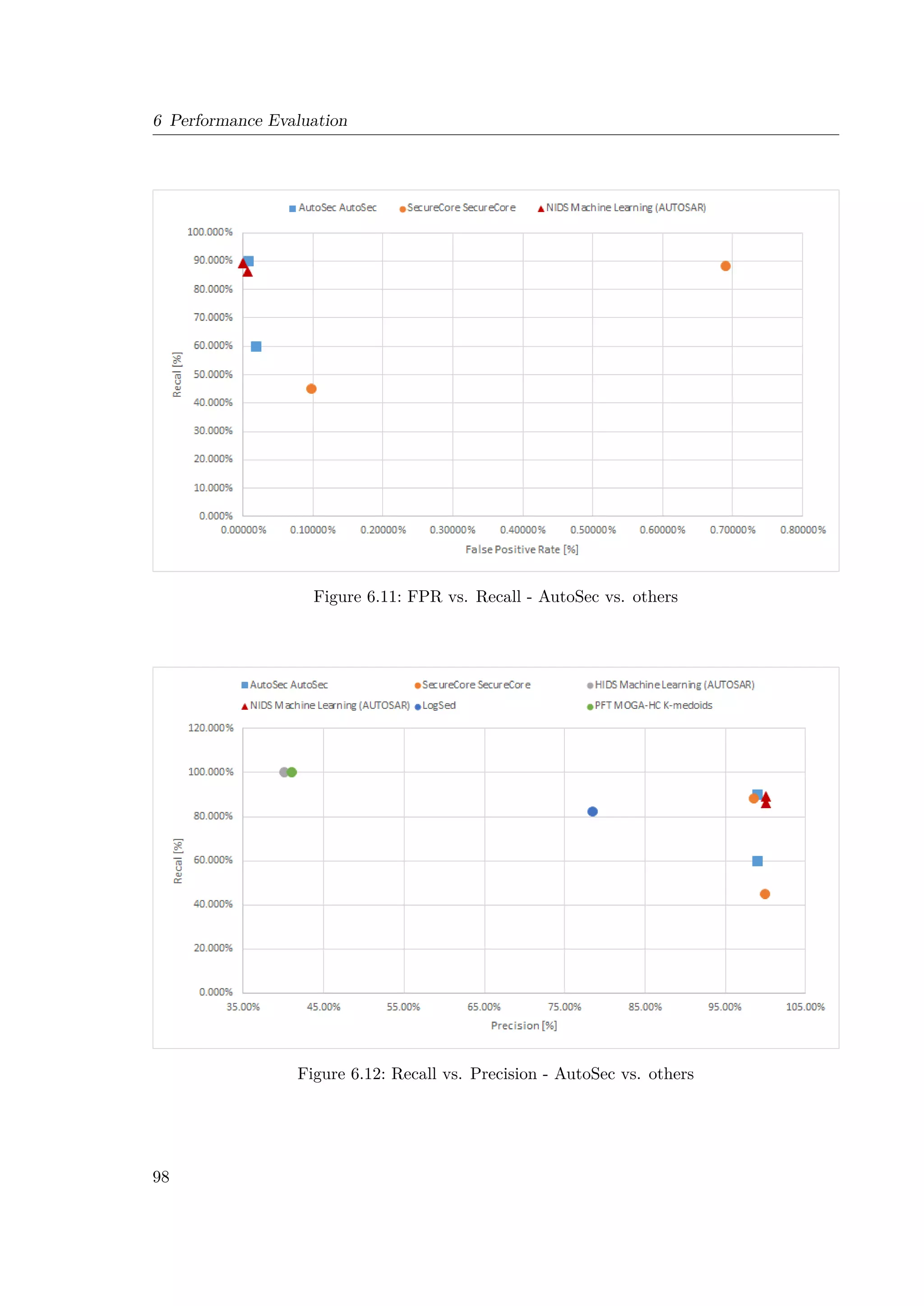
![6.4 Results
tion,Figure 6.12 demonstrates a comparison between AutoSec and following IDS methods -
[cite papers here], which used Recall and Precision as evaluation values. IDS methods that
have been developed for Automotive Industry, mainly for AUTOSAR standard have mark
(AUTOSAR) in addition to their names. The comparison from Figure 6.11 and Figure 6.12
shows that the AutoSec has outperformed other methods under the requirements:
• FPR - minimize
• Recall - maximaize
• Precision - maximize
The AutoSec has outperformed baseline method SecureCore [9] by 10-50 times in FPR reduc-
tion and increased the Recall.
By evaluating algorithm, a conclusion can be reached that the algorithm can successfully de-
tect anomalistic behaviors using multifeature space even. Tradeoff between FPR and Recall
highly depends on the requirements and results that are wanted to be achieved. More about
this topic in the following Chapter 7. Before, reaching the final conclusion. It is important to
evaluate the algorithm overhead.
The overhead is mainly measured in time needed to process AutoSec algorithm. Although
needed processing time is highly dependent on the hardware under which the algorithm will
be running, an insight can be drawn. In majority of cases, MCU are used in ECUs. Thus, the
clock speed is range of hundreds of MHz. In case of the testbed, the speed of used MCU was
120MHz. The algorithm was running on a single core out of three available cores on the used
MCU. The core in use was the core with highest usage, with most Runnables and Events.
The reason is due to fact that at current stage of MICROSAR, each Runnable is mapped to
specific core during a design time and it will not change, during the runtime, the core under
which it is being executed. Thus the overhead of code implementation could have been mea-
sured using internal clock of the MCU for the core where algorithm was running. The results
showed that one run of the algorithm to evaluate instance was in range between 40 and 200
microseconds. The range of execution depends on how many clusters exist for the measuring
point under the evaluation and whether the instance is anomalistic or not. For the instance
that is anomalistic, algorithm would need to measure the distance of the anomaly, in feature
space, to each cluster. Since these calculations take time due to multiple multiplications,
divisions and using square root functions, the execution time requires more computation time
by MCU introducing overhead. Although 200 microseconds does not seems long, put it in
equation that some ECUs can run more than 10000 Runnables, and by instrumenting each
as a measuring point, total overhead would be 2s. Thus, such implementation is not feasible.
Therefore, a risk assessment on Runnables is needed to evaluate which Runnables should have
been instrumented as measuring points due to higher security risk.
Final conclusion on tradeoffs and comparison to the results from [40] will be discussed in the
following Chapter 7.
99](https://image.slidesharecdn.com/milanthesis-220913145214-138d4713/75/Milan_thesis-pdf-119-2048.jpg)

![Chapter 7
Conclusion
Automotive industry is highly competitive environment with no room for errors since safety
and security are highest priority beyond customers’ expectations on comfort of travelling.
Vehicles reached high level of complexity and system dependencies that require extensive
data exchange through various communication channels and mediums. In addition to standard
vehicles features being seen in modern vehicles up-to-day, the interconnectivity of systems will
expand beyond the car by networking vehicles among and with the road infrastructure. Thus,
points of failure and possible access points for malicious parties and attackers are exponentially
increasing. Number of threats to passengers safety and security of the information increases.
The turning point that made OEMs and Tier suppliers to pay more attention to security that
can influence safety of passengers happened in 2015. [2]. Charlie Miller and Chris Valasek
exposed the potential security holes through which an attacker can gain an access to highly
risk elements of the car, such as controlling the engine or disabling braking system, etc. Since
they have published their breakthrough, the security was made the top priority of all vehicle
manufacturers and their developers and suppliers.
The defense against potential attacks on vehicles is fresh field of work with not many known
potential attacks. The system complexity and fast development of those leads to not easily
detectable potential points of breaches by malicious code or an attack. Thus, the object is
to develop an algorithm to detect intrusion in the system, or known as Intrusion Detection
System. Since the vehicle consists out of more than 100 ECUs interconnected among using
different types of communication mediums and protocols, the intrusion can be done in two
distinctive ways: through communication or by direct access to an ECU. Therefore, there are
two type of intrusion detection systems: Network-based IDS and Host-based IDS.
Since, the network attacks are already examined by other fields in computer science, attacks by
direct access to specifically oriented hardware (embedded systems) were not much researched.
Therefore, the scope of the Master Thesis to do a research on what has been done and examine
fields of potential use in automotive industry. When it comes to HIDS, in major scope of
research and papers was the context of the program. Since, the exact attack is unknown,
thus the defense measures against unknown attack is to observe for anomalies in the system.
Therefore, some algorithms in this field make a trace on the order of execution of functions
and commands within the code. Downside appears in areas if something highly rare, but still
normal and verified, happens, can lead to significantly different order of execution and thus
making a method to report further normal execution as an attack. Apart from that, this field
was researched in most of cases when it comes to HIDS.
101](https://image.slidesharecdn.com/milanthesis-220913145214-138d4713/75/Milan_thesis-pdf-121-2048.jpg)
![7 Conclusion
Contrary to order of execution and call flow of functions, timings of executions in the system
were not commonly researched, best to the author’s knowledge. The timing of execution
reflects to evaluating duration of execution of a function. The work in this field of tracing
execution values was done by [9]. As described in Chapter 6, measures used to evaluate
outcomes’ score are FPR, Precision and Recall. In [9] achieved values were:
SecureCore
Lower
Threshold
Higher
Threshold
FPR 0.6897% 0.098%
Precision 98.54% 99.89%
Recall 88.43% 45.12%
Table 7.1: SecureCore evaluation results
TimedCore Runnable
Level
Event Level
FPR 0.018% 0.0075%
Precision 99% 98.95%
Recall 90% 60%
Table 7.2: TimedCore evaluation results
Examining values shown in Table 7.1, it can be seen that FPR needs to be reduced, whilst
Recall to be increased in case of higher threshold. In order to do so, the method proposed
by the Thesis (AutoSec) experimented with other timing features: Start times, preemptions
and duration of preemptions. The novel approach, best to the author’s knowledge, used four
different timing features in a single feature space. Feature space is such that each axis in this
102](https://image.slidesharecdn.com/milanthesis-220913145214-138d4713/75/Milan_thesis-pdf-122-2048.jpg)

![Bibliography
[1] PwC, “The 2017 strategy digital auto report - fast and furious: Why making money
in the “roboconomy” is getting harde,” tech. rep., 2017.
[2] C. Miller and C. Valasek, “Remote exploitation of an unaltered passenger vehicle.” DEF
CON 23, 2015.
[3] M. Weyrich and C. Ebert, “Software engineering for real-time systems.” Lecture Notes
Winter Term 18/19, Oct. 2018.
[4] VectorInformatik, “Introduction to autosar | learning module autosar,” Sept. 2018.
[5] “Autosar exp - layered software architecture release 4.4.0.” https://www.autosar.org/
fileadmin/Releases_TEMP/Classic_Platform_4.4.0/General.zip, 2019. Accessed:
April 2019.
[6] G. C. Buttazzo, Hard Real-Time Computing Systems. Springer US, 2011.
[7] “Virtual integration and test of autosar systems.” https://assets.vector.com/cms/
content/events/2018/Webinars18/Vector_Webinar_vVIRTUALtarget_20180124.
pdf, Sept. 2017. Vector Informatik GmbH.
[8] “Autosar tps - specification of timing extensions release 4.4.0.” https:
//www.autosar.org/fileadmin/Releases_TEMP/Classic_Platform_4.4.0/
MethodologyAndTemplates.zip, 2019. Accessed: April 2019.
[9] M.-K. Yoon, S. Mohan, J. Choi, J.-E. Kim, and L. Sha, “SecureCore: A multicore-based
intrusion detection architecture for real-time embedded systems,” in 2013 IEEE 19th
Real-Time and Embedded Technology and Applications Symposium (RTAS), IEEE, apr
2013.
[10] V. I. GmbH, User Manual TA Tool Suite (Release 19.1.0).
[11] “Ericsson - internet of things forecast.” https://www.ericsson.com/en/mobility-
report/internet-of-things-forecast. Accessed: 2019-10-23.
[12] “Bmw group and daimler ag invest more than 1 billion in joint mobility services
provider.” https://www.press.bmwgroup.com/global/article/detail/T0292204EN/
bmw-group-and-daimler-ag-invest-more-than-%E2%82%AC1-billion-in-joint-
mobility-services-provider?language=en. Accessed: 2019-10-23.
105](https://image.slidesharecdn.com/milanthesis-220913145214-138d4713/75/Milan_thesis-pdf-125-2048.jpg)
![Bibliography
[13] “Iso 26262-1:2018.” https://www.iso.org/standard/68383.html, 2018. Accessed:
April 2019.
[14] S. Biswas, R. Tatchikou, and F. Dion, “Vehicle-to-vehicle wireless communication pro-
tocols for enhancing highway traffic safety,” IEEE Communications Magazine, vol. 44,
pp. 74–82, jan 2006.
[15] X. Yang, J. Liu, F. Zhao, and N. Vaidya, “A vehicle-to-vehicle communication protocol for
cooperative collision warning,” in The First Annual International Conference on Mobile
and Ubiquitous Systems: Networking and Services, 2004. MOBIQUITOUS 2004., IEEE,
2004.
[16] S. Furst, “Challenges in the design of automotive software,” in 2010 Design, Automation
Test in Europe Conference Exhibition (DATE 2010), IEEE, mar 2010.
[17] “Autosar - history.” https://www.autosar.org/about/history/. Accessed: April 2019.
[18] A. Patzer, “Data recording for adas development,” Mar. 2017.
[19] M. Staron, Automotive Software Architectures. Springer International Publishing, 2017.
[20] “Autosar exp - application interfaces user guide release 4.4.0.” https://www.autosar.
org/fileadmin/Releases_TEMP/Classic_Platform_4.4.0/General.zip, 2019. Ac-
cessed: April 2019.
[21] P. Marwedel, Embedded System Design. Springer International Publishing, 2018.
[22] J. W. S. Liu, Real-Time Systems. Integre Technical Publishing Co., Inc, 2000.
[23] “Autosar tr - recommended methods and practices for timing analysis and design within
the autosar development process release 4.4.0.” https://www.autosar.org/fileadmin/
Releases_TEMP/Classic_Platform_4.4.0/BSWGeneral.zip, 2019. Accessed: April
2019.
[24] D. P. Möller and R. E. Haas, Guide to Automotive Connectivity and Cybersecurity.
Springer International Publishing, 2019.
[25] A. Nasser and D. Ma, “Defending AUTOSAR safety critical systems against code reuse
attacks,” in Proceedings of the ACM Workshop on Automotive Cybersecurity - AutoSec
19, ACM Press, 2019.
[26] M. E. M. Weber, Untersuchungen zur Anomalieerkennung in automotive Steuergeräten
durch verteilte Observer mit Fokus auf die Plausibilisierung von Kommunikationssig-
nalen. phdthesis, Elektrotechnik und Informationstechnik des Karlsruher Instituts für
Technologie (KIT), Mar. 2019.
[27] M. Yoon, S. Mohan, J. Choi, M. Christodorescu, and L. Sha, “Learning execution contexts
from system call distribution for anomaly detection in smart embedded system,” in Proc.
106](https://image.slidesharecdn.com/milanthesis-220913145214-138d4713/75/Milan_thesis-pdf-126-2048.jpg)
![Bibliography
IEEE/ACM Second Int. Conf. Internet-of-Things Design and Implementation (IoTDI),
pp. 191–196, Apr. 2017.
[28] P. A. Almeida, “Evaluation and prototypical implementation of machine learning to
detect ecu misbehavior,” Master’s thesis, Fakultät für Elektrotechnik, Insttitu für Technik
der Informationsverarbeitung (ITIV), Aug. 2017.
[29] J.-Y. Ding, K. You, S. Song, and C. Wu, “Likelihood ratio-based scheduler for secure
detection in cyber physical systems,” IEEE Transactions on Control of Network Systems,
vol. 5, pp. 991–1002, sep 2018.
[30] C. Bernardeschi, M. D. Natale, G. Dini, and M. Palmieri, “Verifying data secure flow
in AUTOSAR models,” Journal of Computer Virology and Hacking Techniques, vol. 14,
pp. 269–289, mar 2018.
[31] F.-J. Wang, A. Chang, and T. Lu, “Improving workflow anomaly detection with a c-tree,”
in 2017 IEEE 41st Annual Computer Software and Applications Conference (COMP-
SAC), IEEE, jul 2017.
[32] L. Wang, X. Wang, Z. Zhou, Q. Liu, and H. Yang, “Architectural-enhanced intrusion
detection and memory authentication schemes in embedded systems,” in 2010 IEEE
International Conference on Information Theory and Information Security, IEEE, dec
2010.
[33] T. Jia, L. Yang, P. Chen, Y. Li, F. Meng, and J. Xu, “LogSed: Anomaly diagnosis
through mining time-weighted control flow graph in logs,” in 2017 IEEE 10th Interna-
tional Conference on Cloud Computing (CLOUD), IEEE, jun 2017.
[34] M. Rahmatian, H. Kooti, I. G. Harris, and E. Bozorgzadeh, “Hardware-assisted detection
of malicious software in embedded systems,” IEEE Embedded Systems Letters, vol. 4,
pp. 94–97, dec 2012.
[35] D. Pfau, N. Bartlett, and F. Wood, “Probabilistic deterministic infinite automata,” in
Advances in Neural Information Processing Systems 23 (J. D. Lafferty, C. K. I. Williams,
J. Shawe-Taylor, R. S. Zemel, and A. Culotta, eds.), pp. 1930–1938, Curran Associates,
Inc., 2010.
[36] W. Zhang, F. Bastani, I.-L. Yen, K. Hulin, F. Bastani, and L. Khan, “Real-time anomaly
detection in streams of execution traces,” in 2012 IEEE 14th International Symposium
on High-Assurance Systems Engineering, IEEE, oct 2012.
[37] L. Fei and S. P. Midkiff, “Artemis,” in Proceedings of the 2006 ACM SIGPLAN conference
on Programming language design and implementation - PLDI 06, ACM Press, 2006.
[38] E. White, Making Embedded Systems. O’Reilly UK Ltd., 2011.
[39] S. Lloyd, “Least squares quantization in PCM,” IEEE Transactions on Information The-
ory, vol. 28, pp. 129–137, mar 1982.
107](https://image.slidesharecdn.com/milanthesis-220913145214-138d4713/75/Milan_thesis-pdf-127-2048.jpg)
![Bibliography
[40] C. C. Aggarwal, Outlier Analysis. Springer International Publishing, 2017.
[41] A. Mucherino, P. J. Papajorgji, and P. M. Pardalos, “k-nearest neighbor classification,”
in Data Mining in Agriculture, pp. 83–106, Springer New York, 2009.
[42] U. von Luxburg, “A tutorial on spectral clustering,” Statistics and Computing, vol. 17,
pp. 395–416, aug 2007.
[43] B. J. Frey and D. Dueck, “Clustering by passing messages between data points,” Science,
vol. 315, pp. 972–976, feb 2007.
[44] C. et al., “Gaussian mixture models,” in Encyclopedia of Biometrics, pp. 659–663,
Springer US, 2009.
[45] M. Ester, H.-P. Kriegel, J. Sander, X. Xu, et al., “A density-based algorithm for dis-
covering clusters in large spatial databases with noise.,” in Kdd, vol. 96, pp. 226–231,
1996.
[46] R. Paredes and E. Chávez, “Using the k-nearest neighbor graph for proximity searching
in metric spaces,” in String Processing and Information Retrieval, pp. 127–138, Springer
Berlin Heidelberg, 2005.
108](https://image.slidesharecdn.com/milanthesis-220913145214-138d4713/75/Milan_thesis-pdf-128-2048.jpg)


