Downloaded 18 times


![Bayesian Methods
Mk = [Y1, Y2, ., Yk] (2.4)
The objective of this formulation is to estimate the current state Xk based on the measure-
ment Yk. As the model and the measurements are corrupted with noise it is required the
problem of state estimate reduces to estimating the probability density function p(Xk|Mk).
Since estimating p(Xk|Mk) is itself not easy, so the more simplified problem is to determine
the moments of Xk. Mathematically, this can be written as:
µ =
∫
Xkp(Xk|Mk)dXk (2.5)
σ =
∫
(Xk − µ)T
(Xk − µ)p(Xk|Mk)dXk (2.6)
where µ and σ are the first moment or mean and the second moment or variance of the pdf
p(Xk|Mk) respectively.
In the following, a detailed derivation of the recursive Bayesian Estimation is presented,
which underlines the principles of sequential Bayesian filter. Two assumptions are used to
derive the recursive Bayesian Filter.
• The sates follow a first order Markov process
p(Xk|X0:k−1) = p(Xk|Xk−1); (2.7)
• The observations are independent of the given states.
At any time t, the posterior is given by the Bayes theorem as
p(X0:t|Y1:t) =
p(Y1:t|X0:t)p(X0:t)
∫
p(Y1:t|X0:t)p(X0:t)dX0:t
(2.8)
The recursive equation can be obtained as
p(X0:t+1|Y1:t+1) = p(X0:t|Y1:t)
p(Yt+1|Xt+1)p(Xt+1|Xt)
p(Yt+1|Y1:t)
(2.9)
The following recursive relations are used for prediction and updating
11](https://image.slidesharecdn.com/bbb51381-8346-4dce-8bb4-393bf7d891de-150830202310-lva1-app6892/85/thesis-22-320.jpg)
![Monte Carlo Methods
2.2 Monte Carlo Methods
The underlying principle of the MC methods is that they utilize Markov chain theory.
The resulting empirical distribution converges to the desired posterior distribution through
random sampling. The method is widely used in signal processing where one is interested
in determining the moment of the stochastic signal f(X) with respect to some underlying
probabilistic distribution p(X). However the similar concept is used in system identification
problem where one is interested to estimate the expected values of the system parameters.
The methods have the great advantage since these are not subject to constraints of linear-
ity and Gaussianity. The methods as well have appealing convergence properties. Several
variants of MC methods are available in the literature. This includes Perfect Monte carlo
sampling,Sequential importance sampling, Sequential importance resampling and the Boot-
strap particle filter. The following section presents the mathematical formulation of each of
the method. The concept has been illustrated by solving single degree of freedom oscillator
at the end of the chapter.
2.2.1 Perfect Sampling & Sequential Importance Sampling (SIS)
Monte Carlo methods use statistical sampling and estimation techniques to evaluate the
solutions to mathematical problems. The underlying mathematical concept of Monte Carlo
approximation is simple. Consider the statistical problem of estimating the expected value
of E[f(x)] with respect to some probabilistic distribution p(X):
E[f(X)] =
∫
f(X)p(X)dX (2.21)
Here the motivation is to integrate the above expression using stochastic sampling techniques
rather than using the numerical integration techniques. Such a practice is useful to estimate
complex integral where it is difficult to obtain the closed form solution. In MC approach, the
required distribution is represented by random samples rather than analytic function. The
approximation becomes better and more exact when the number of number of such random
samples increases. Thus, MC integration evaluates Eq 2.21 by drawing samples X(i) from
p(X). Assuming perfect sampling, the empirical distribution is given by
p(x) =
1
N
N∑
i=1
δ(X − X(i)) (2.22)
14](https://image.slidesharecdn.com/bbb51381-8346-4dce-8bb4-393bf7d891de-150830202310-lva1-app6892/85/thesis-25-320.jpg)
![Monte Carlo Methods
The above equation can be substituted to give
E[f(x)] =
∫
f(X)p(X)dX≃
1
N
N∑
i=1
f(X(i)) (2.23)
Generalization of this approach is known as Importance sampling where the integral is writ-
ten as
I =
∫
p(x)dx =
∫
p(x)
q(x)
q(x)dx (2.24)
given ∫
q(x)dx = 1 (2.25)
Here q(X) is known as the importance sampling distribution since it samples p(X) non-
uniformly giving more importance to some values of p(x). The Eq 2.24 can be written
as
I = Eq[
p(X)
q(X)
] =
1
N
N∑
i=1
p(X(i))
q(X(i))
(2.26)
where X(i) are drawn from the importance distribution q(.).
The central theme of importance sampling is to choose importance distribution q(.) which
can approximate the target distribution p(.) as close as possible. Using the concept of
importance sampling, it is possible to approximate the posterior distribution. Since it is
generally not easy to sample from the posterior, we use importance sampling coupled with
an easy to sample proposal distribution q(Xt|Yt).This is one of the most important steps
of the Bayesian importance sampling methodology. Using the importance sampling concept
the mean of f(Xt) can be estimated as follows:
E[f(Xt)] =
∫
f(Xt)p(Xt|Yt)dXt (2.27)
where (Xt|Yt) is the posterior distribution. Here, we insert the importance proposal density
function q(Xt|Yt) such that the estimate becomes
F(t) = E[f(Xt)] =
∫
f(Xt)
p(Xt|Yt)
q(Xt|Yt)
q(Xt|Yt)dXt (2.28)
15](https://image.slidesharecdn.com/bbb51381-8346-4dce-8bb4-393bf7d891de-150830202310-lva1-app6892/85/thesis-26-320.jpg)
![Monte Carlo Methods
Now using Eq 2.18 (Bayes Rule) to the posterior distribution and defining the weighting
function as
˜W(t) =
p(Xt|Yt)
q(Xt|Yt)
=
p(Yt|Xt)p(Xt)
p(Yt)q(Xt|Yt)
(2.29)
Calculation of ˜W(t) requires the knowledge of the normalizing constant p(Yt) which is given
by
p(Yt) =
∫
p(Yt|Xt)p(Xt)dXt (2.30)
This normalizing constant is generally not available and hence the new weight W(t) can be
defined by substituting Eq 2.29 into Eq 2.28.
F(t) =
1
p(Yt)
∫
f(Xt)
p(Yt|Xt)p(Xt)
q(Xt|Yt)
q(Xt|Yt)dXt
=
1
p(Yt)
∫
W(t)f(Xt)q(Xt|Yt)dXt
=
1
p(yt)
Eq[W(t)f(Xt)]
(2.31)
The above equation can be also be written as:
W(t)q(Xt|Yt) = p(Yt|Xt)p(Xt) (2.32)
Thus, the normalizing constant in Eq 2.30 can be replaced by 2.32
F(t) =
Eq[W(t)f(Xt)]
p(Yt)
=
Eq[W(t)f(Xt)]
∫
W(t)q(Xt|Yt)
=
Eq[W(t)f(Xt)]
Eq[W(t)]
(2.33)
Now, if the samples are drawn from the distribution q(Xt|Yt), from perfect sampling distri-
16](https://image.slidesharecdn.com/bbb51381-8346-4dce-8bb4-393bf7d891de-150830202310-lva1-app6892/85/thesis-27-320.jpg)
![Monte Carlo Methods
q(Xi
k|Xi
0:k−1, Y1:k) = p(Xi
k|Xi
k−1, Yk) (2.49)
By substituting Eq 2.49 in Eq 2.44 the updated weight becomes
wi
k∝wi
k−1p(Yk|Xi
k−1), (2.50)
This optimal importance distribution can be used when the state space is finite.The present
report also uses the similar assumption of importance density. However, the report deals
with the problem of system identification where we are more interested in identifying the
system parameters rather then tracking the sate vector.
The algorithm can be implemented in the following manner
• Draw particles Xi
k from the importance distribution
Xi
k∼q(Xk|Xi
0:k−1, Y1:k), i = 1, ..., N (2.51)
• The new weights can be calculated from Eq 2.44 for all the particles an normalize them
to unity.
• If Neff calculated in Eq 2.48 becomes too low, perform the resampling step.
• Interpret each weight wi
k as the probability of obtaining the sample index i in the set
Xi
k for [i = 1, . . . ,N].
• Draw N samples from that discrete distribution and replace the old sample set with
this new one.
• Set all weights to the constant value wi
k = 1
N
.
The Bootstrap filter is a special case of SIR filter where the dynamic model is used as impor-
tance distribution as in Eq 2.50 and the resampling is done at each step. A brief algorithm is
presented here for a more clear illustration. However, the problem formulation section gives
the detailed implementation of Bootstrap filter to System identification problem.
• Draw point Xi
k from the dynamic model
Xi
k ∼ p(Xk|Xi
k−1)i = 1, ..., N (2.52)
20](https://image.slidesharecdn.com/bbb51381-8346-4dce-8bb4-393bf7d891de-150830202310-lva1-app6892/85/thesis-31-320.jpg)
![Monte Carlo Methods
• Calculate new weights and normalize them to unity.
wi
k ∝ p(Yk|Xi
k)i = 1, ..., N (2.53)
• Perform resampling after each iteration.
One of the important steps in the above algorithm is resampling from the discrete probability
mass function containing the normalized weights. Resampling ensures that particles with
larger weights are more likely to be preserved than particles with smaller weights. Although
the resampling solves the degeneracy, but it introduces sample impoverishment which is
explained through an example problem solved at the end of the chapter. There are wide
variety of resampling algorithms available in the literature (Li, 2013). This report discusses
the traditional resampling strategies as well as the comparative study of these algorithms in
light of the system identification problem. The traditional resampling algorithms discussed
are namely Multinomial or simple resampling, Systematic & Stratified resampling and Wheel
resampling. A brief description of the algorithms is presented below
Multinomial Resampling
Multinomial Resampling also known as binary search resampling or simple resampling is
one of the simplest of the resampling algorithms which generates N random numbers un
t
and use them to sample particles from the array containing the normalized weights of the
particles wi
. The cumulative sum of the weights is done to select the interval in which the
random number lies. The selection of the mth
particle must satisfy the following equation
m−1∑
i=1
wi < un
t <
m∑
i=1
wi (2.54)
Since the sampling of each particle is purely random so a given particle can be sampled a
minimum of zero times and a maximum of N times.
Stratified Resampling
Stratified sampling divides the total population in sub-populations or the interval of (0,1]
into 1
N
equal intervals. Hence the disjoint sub-intervals are (0, 1
N
] ∪ ( 1
N
, 2
N
] ∪ (1 − 1
N
, 1]. The
21](https://image.slidesharecdn.com/bbb51381-8346-4dce-8bb4-393bf7d891de-150830202310-lva1-app6892/85/thesis-32-320.jpg)
![Monte Carlo Methods
random numbers are drawn from each of the sub-intervals as
un
= U(
n − 1
N
,
n
N
), n = 1, 2....., N (2.55)
After the random number is generated, each sub-interval is tested using cumulative sum of
normalized weights as shown in Eq 2.54
Systematic Resampling
Systematic resampling is similar to stratified resampling where the first random number
is generated from the uniform distribution between (0, 1
N
]. After this the random numbers
are generated deterministically using the equation
un
t = u1
t +
n − 1
N
, n = 2, 3....., N (2.56)
The literature suggests that the systematic resampling is computationallye more efficient
due to smaller number of random numbers that have to be generated Li (2013).
Wheel Resampling
In this resampling method the particles are represented as big wheel with each particle
occupying the circumference proportional to its normalized weight. Particles with bigger
weight occupy more space and the ones with smaller occupy smaller space. An iterative loop
is run for N times where particles will be chosen in proportion to their circumference on the
circle.
Although the resampling step reduces the degeneracy, it introduces various problems. To
begin with, it limits the opportunity to parallelize since all the particle must be combined.
Moreover, resampling introduces the problem of sample impoverishment as particles having
higher weights are selected multiple number of times. This also leads to lack of diversity
among the particles. For the case of very small process noise, all the particles will collapse
to a single point. Different researchers have tried various schemes to deal with sample
impoverishment(Nasrellah and Manohar, 2011). The following section demonstrates the
implementation of the algorithm to a single degree of freedom (SODF) oscillator.
22](https://image.slidesharecdn.com/bbb51381-8346-4dce-8bb4-393bf7d891de-150830202310-lva1-app6892/85/thesis-33-320.jpg)
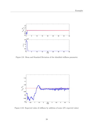
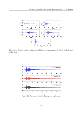
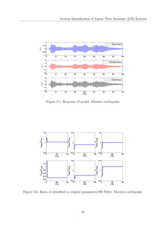
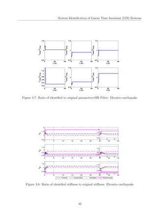
![Examples
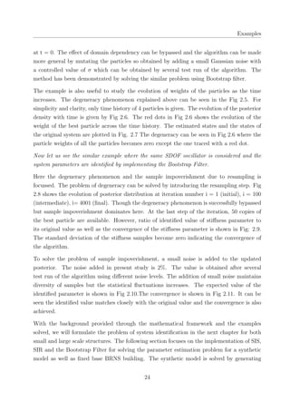
2.3 Examples
In this section numerical examples are presented to demonstrate the implementation of
particle filters. We consider a single-degree-of-freedom (SDOF) oscillator excited by Elcentro
earthquake. We start with a simple problem which aims at identifying the stiffness of the
SDOF oscillator, given the response of the oscillator to earthquake excitation. Both SIS and
Bootstrap filters have been used to solve this example. The measurement data has been
synthetically generated by solving the forward problem by assuming known values of the
system parameters. Once the synthetic measurements are known, the inverse problem is
solved using various time domain methods described above. A schematic diagram of the
oscillator is shown in Fig 2.1. The governing equation of motion of SDOF oscillator is given
by the second order differential equation as:
M ¨u(t) + C ˙u(t) + Ku(t) = −M ¨ug(t) (2.57)
where , M is the Mass, C is the damping, K is the stiffness, ¨ug(t) is the acceleration due
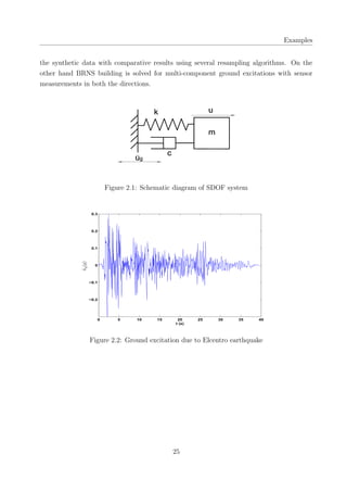
to the ground motion. Here we have considered the ground motion due to 1940 Elcentro
earthquake. Elcentro was the first earthquake to be recorded by strong motion seismograph
and had the magnitude of 6.9. For solving the forward problem, M is assumed to be 40 kg,
C is assumed as 15 N-s and the stiffness value is assumed as 6 × 10⁴
(N/m). The natural
frequency of the oscillator is 38.72 rad/s. The problem in hand is to identify the stiffness
of the SDOF oscillator. The forward problem has been solved by using the time marching
algorithm to obtain the response numerically. We use β Newmark algorithm which is an
implicit unconditionally stable time marching algorithm (Newmark, 1959). The MATLAB
code forβ Newmark algorithm has been provided in the appendix.
The ground excitation due to the Elcentro earthquake has been plotted in Fig 2.2. The
overall duration of the excitation is 40s. The time step considered in the analysis for solving
the forward problem is 0.01 sec. Hence the total number of data points are 4000. The
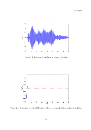
response of the oscillator is shown in Fig 2.3
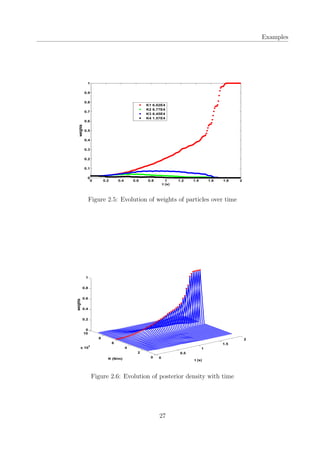
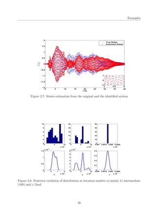
The SIS filter is now applied to identify the stiffness value of the oscillator. The total number
of particles considered are 50. The initial values of the stiffness are generated in the domain
of [10000,90000] from the uniform distribution. The algorithm is dependent on the parameter
values generated at time t = 0. The identified value over the entire time history is shown in
the Fig 2.4
Hence, the algorithm acts as a filter and returns the best value among all the values generated
23](https://image.slidesharecdn.com/bbb51381-8346-4dce-8bb4-393bf7d891de-150830202310-lva1-app6892/85/thesis-34-320.jpg)
![System Identification of Linear Time Invariant (LTI) Systems
the updated posteriori distribution of the state. More samples are generated from the region
where the likelihood is greater. To solve the problem for identification of parameters, ϕ, the
state vector can be augmented as Xk = [Zkϕk] and assuming model noise as the sequence
of i.i.d random variable wk, the above Eq 3.2 can be discretized in the form of Eq 2.2. The
dimension of the problem is equal to sum of vector Z and ϕ. Hence one is able to identify the
state vector as well as the parameters. In the system identification problem we are generally
interested in identifying the system parameters rather than tracking the state of the system.
(Nasrellah and Manohar, 2011) suggested that a larger computational effort can be reduced
by formulating the problem in terms of system parameters . Hence,the systems which remain
invariant with time, the system equation can be expressed as:
dϕ
dt
= 0
ϕj(0) = ϕ0 j = 1, 2.........n
(3.3)
where ϕ0 is the value of the value of the system parameters at time t = 0. The discrete
version of the equation can be presented as
ϕk+1 = ϕk + wk (3.4)
where ϕk is the system parameters at time k, wk is the model noise. The corresponding
measurement equation can be written as
Yk = hk(ϕk) + vk (3.5)
The advantage of the above modeling is that it reduces the dimensions of the state vector
which is equal to dimension of the ϕ vector and hence the associated computational effort.
The MATLAB code for the bootstrap particle filter for system identification of LTI system
is given in the appendix. However, the implementation and the key steps involved in the
algorithm are discussed below.
1. The algorithm starts with simulating N samples for all the parameters to be identified
(ϕ0), from the assumed pdf of (ϕ0) at the time instant t = 0. The random particles are
generated in a suitable domain identified by the upper and the lower bounds. These
are also known as the prior estimates.
2. The next step involves solving N linear forward problems, Eq 3.1 corresponding to
each of the prior estimate ϕk−1. The forward problems are solved using the β Newmark
32](https://image.slidesharecdn.com/bbb51381-8346-4dce-8bb4-393bf7d891de-150830202310-lva1-app6892/85/thesis-43-320.jpg)
![Appendix A
% exct = El Centro EW;
% time = El Centro EW(:,1);
% plot(exct(:,1),exct(:,2));
% xlabel('T (s)'); ylabel('$ddot{X} {g}(m/{sˆ2})$ ','interpreter','latex')
% Inc = zeros(1,3);
% [U,Ud,Udd] = Newmark Beta MDOF(m,k,c,Inc,exct);
% response = [time Udd'];
% save sis measurement.dat −ascii response
%**********************************************************************
% Inverse Problem for System Identification using SIS Filter:
% =================================================================
load sis measurement.dat
load El Centro EW.dat
exct = El Centro EW;
time = sis measurement(:,1);
t = length(time);
acc = sis measurement(:,2);
k inv = 10000 + (80000).*rand(N,1); % particles from uniform dist.
sorted = sort(k inv); % sorted value of particles
k =1;
for i = 1:N
w(i,k) = 1/N;
end
wk(:,k) = w(:,k)./sum(w(:,k));
Inc prior(:,:,N) = zeros(1,3);
for k = 2:t
k
for i = 1:N
[Inc update] = Newmark Beta MDOF instant(m,k inv(i),c,...
Inc prior(:,:,i),exct,k,0.5,1/6);
C(:,:,i)= Inc update;
% Estimate Likelihood of Simulation:
% ==================================
w(i,k) = wk(i,k−1)*(1/sqrt(2*pi*x R)) * exp(−((acc(k)...
− Inc update(1,3))ˆ2)/(2*(x R)));
end
63](https://image.slidesharecdn.com/bbb51381-8346-4dce-8bb4-393bf7d891de-150830202310-lva1-app6892/85/thesis-74-320.jpg)
![Appendix A
% Updating the particle weights:
% ==================================
wk(:,k) = w(:,k)./sum(w(:,k));
Inc prior = C;
k estimate = 0;
% Estimating the parmeter value:
% ==================================
for i = 1:N
k estimate = k estimate + wk(i,k)*k inv(i);
end
k iden(k−1) = k estimate/k or;
end
%**********************************************************************
% Plots
% =================================================================
% plot(time(2:t),k iden);
% xlabel('T (s)'); ylabel('K (kN/m)');
% plot(time(1:200),wk(30,1:200),'*r',time(1:200),wk(9,1:200),...
...'*g',time(1:200),wk(2,1:200),'*b',time(1:200),wk(4,1:200),'*k')
% xlabel('T (s)');ylabel('weights')
% legend('6.02E4','6.77E4','6.45E4','1.57E4')
% [ksort,index] = sort(k inv);
% for i = 1:4:200
% tp = ((i−1)*0.01)*ones(50,1);
% plot3(tp,ksort,wk(index,i),'b')
% xlabel('T (s)'); ylabel('K (N/m)'); zlabel('weights');
% hold on
% end
% hold on
% for i = 1:4:200
% plot3(time(i),k inv(30),wk(30,i),'.r','Markersize',14)
% hold on
% end
64](https://image.slidesharecdn.com/bbb51381-8346-4dce-8bb4-393bf7d891de-150830202310-lva1-app6892/85/thesis-75-320.jpg)
![Appendix A
MATLAB code for parameter identification of synthetic model using Sequential
Importance Sampling (SIS) filter
This code solves the parameter identification for the three storied shear building synthetic
model using SIS Filter.
% =========================================================================
% PROGRAMMER : ANSHUL GOYAL
% DATE : 02.01.2014(Last modified: 25:01:2014)
% ABSTRACT : Sequential Importance Sampling (SIS) filter Code for
% parameter estimation of laboratory model
% =========================================================================
clear all
close all
clc
% *************************************************************************
% Input Section:
% ==============
m = [15.2 15.2 15.2];
c = [19.032 34.173 33.63];
k = [41987 76842 74812];
N = 100;
x R = 0.001;
% ***********************************************************************
% Forward Problem for Synthetic Measurements:
% ===========================================
% load Elcentro X.dat
% exct = Elcentro X;
% time = Elcentro X(:,1);
% Inc = zeros(3,3);
% [M mat,K mat,C mat]=LTI System Matrices(m,k,c);
% [U,Ud,Udd] = Newmark Beta MDOF(M mat,K mat,C mat,Inc,exct);
% response = [time Udd'];
% save resp elcentro.dat −ascii response
% ***********************************************************************
% Eigen Analysis of laboratory model:
% ===========================================
65](https://image.slidesharecdn.com/bbb51381-8346-4dce-8bb4-393bf7d891de-150830202310-lva1-app6892/85/thesis-76-320.jpg)
![Appendix A
[Phi,D] = eig(K mat,M mat);
wn or = sqrt(diag(D))/(2*pi); % Natural fequency in Hz
%**********************************************************************
% Inverse Problem for System Identification using SIS Filter:
% =================================================================
load resp elcentro.dat
load Elcentro X.dat
load test stiffness 3dof elcentro.dat % data file containing 100 samples
rand sample = test stiffness 3dof elcentro;
exct = Elcentro X;
time = resp elcentro(:,1);
acc1 = resp elcentro(:,2);
Inc = zeros(3,3);
% Simulating particles
% ==================================
% k1 = 10000 + (80000).*rand(N,1);
% k2 = 10000 + (80000).*rand(N,1);
% k3 = 10000 + (80000).*rand(N,1);
% c1 = 50.*rand(N,1);
% c2 = 50.*rand(N,1);
% c3 = 50.*rand(N,1);
% Defining initial weights
% ==================================
q =1;
for i = 1:N
w1(i,q) = 1/N;
w2(i,q) = 1/N;
w3(i,q) = 1/N;
end
wk(:,q) = w1(:,q)./sum(w1(:,q));
Inc prior(:,:,N) = zeros(3,3);
for q = 2:length(time)
q
for ii = 1:N
m = [15.2 15.2 15.2];
k = [rand sample(ii,1) rand sample(ii,2) rand sample(ii,3)];
66](https://image.slidesharecdn.com/bbb51381-8346-4dce-8bb4-393bf7d891de-150830202310-lva1-app6892/85/thesis-77-320.jpg)
![Appendix A
c = [rand sample(ii,4) rand sample(ii,5) rand sample(ii,6)];
[M mat,K mat,C mat]=LTI System Matrices(m,k,c);
[Inc update] = Newmark Beta MDOF instant(M mat,K mat,C mat,...
Inc prior(:,:,ii),exct,q,0.5,1/6);
C(:,:,ii)= Inc update;
% Estimate Likelihood of Simulation:
% ==================================
w1(ii,q) = wk(ii,q−1)*(1/sqrt(2*pi*x R)) * exp(−((acc1(q) −...
Inc update(1,3))ˆ2)/(2*(x R)));
end
% Updating the particle weights:
% ==================================
w = w1;
Inc prior = C;
wk(:,q) = w(:,q)./sum(w(:,q));
% Estimating and storing the parameter values:
% ==================================
k1 iden = 0;
k2 iden = 0;
k3 iden = 0;
c1 iden = 0;
c2 iden = 0;
c3 iden = 0;
for ii = 1:N
k1 iden = k1 iden + wk(ii,q)*rand sample(ii,1);
k2 iden = k2 iden + wk(ii,q)*rand sample(ii,2);
k3 iden = k3 iden + wk(ii,q)*rand sample(ii,3);
c1 iden = c1 iden + wk(ii,q)*rand sample(ii,4);
c2 iden = c2 iden + wk(ii,q)*rand sample(ii,5);
c3 iden = c3 iden + wk(ii,q)*rand sample(ii,6);
end
k11 iden(q−1) = k1 iden;
k22 iden(q−1) = k2 iden;
k33 iden(q−1) = k3 iden;
c11 iden(q−1) = c1 iden;
c22 iden(q−1) = c2 iden;
67](https://image.slidesharecdn.com/bbb51381-8346-4dce-8bb4-393bf7d891de-150830202310-lva1-app6892/85/thesis-78-320.jpg)
![Appendix A
close all
clc
% *************************************************************************
% Input Section:
% ==============
m = [15.2 15.2 15.2];
c = [19.032 34.173 33.63];
k = [41987 76842 74812];
N = 100;
x R = 0.001;
% ***********************************************************************
% Forward Problem for Synthetic Measurements:
% ===========================================
% load ChiChi X.dat
% exct = ChiChi X;
% time = ChiChi X(:,1);
% Inc = zeros(3,3);
% [M mat,K mat,C mat]=LTI System Matrices(m,k,c);
% [U,Ud,Udd] = Newmark Beta MDOF(M mat,K mat,C mat,Inc,exct);
% response = [time Udd'];
% save resp ChiChi.dat −ascii response
% ***********************************************************************
% Eigen Analysis of laboratory model:
% ===========================================
[Phi,D] = eig(K mat,M mat);
wn or = sqrt(diag(D))/(2*pi); % Natural fequency in Hz
%**********************************************************************
% Inverse Problem for System Identification using SIS Filter:
% =================================================================
tm = cputime;
load resp ChiChi.dat
load ChiChi X.dat
load test stiffness 3dof ChiChi.dat % data file containing 100 samples
rand sample = test stiffness 3dof ChiChi;
exct = ChiChi X;
time = resp ChiChi(:,1);
acc1 = resp ChiChi(:,2);
69](https://image.slidesharecdn.com/bbb51381-8346-4dce-8bb4-393bf7d891de-150830202310-lva1-app6892/85/thesis-80-320.jpg)
![Appendix A
acc2 = resp ChiChi(:,3);
acc3 = resp ChiChi(:,4);
Inc = zeros(3,3);
% Simulating particles
% ==================================
% k1 = 10000 + (80000).*rand(N,1);
% k2 = 10000 + (80000).*rand(N,1);
% k3 = 10000 + (80000).*rand(N,1);
% c1 = 50.*rand(N,1);
% c2 = 50.*rand(N,1);
% c3 = 50.*rand(N,1);
% Defining initial weights
% ==================================
q =1;
for i = 1:N
w1(i,q) = 1/N;
w2(i,q) = 1/N;
w3(i,q) = 1/N;
end
wk(:,q) = w1(:,q)./sum(w1(:,q));
Inc prior(:,:,N) = zeros(3,3);
for q = 2:500
q
for ii = 1:N
m = [15.2 15.2 15.2];
k = [rand sample(ii,1) rand sample(ii,2) rand sample(ii,3)];
c = [rand sample(ii,4) rand sample(ii,5) rand sample(ii,6)];
[M mat,K mat,C mat]=LTI System Matrices(m,k,c);
[Inc update] = Newmark Beta MDOF instant(M mat,K mat,C mat,...
Inc prior(:,:,ii),exct,q,0.5,1/6);
C(:,:,ii)= Inc update;
% Estimate Likelihood of Simulation:
% ==================================
w1(ii,q) = wk(ii,q−1)*(1/sqrt(2*pi*x R)) * exp(−((acc1(q) −...
Inc update(1,3))ˆ2)/(2*(x R)))*(1/sqrt(2*pi*x R)) *....
exp(−((acc2(q) − Inc update(2,3))ˆ2)/(2*(x R)))...
70](https://image.slidesharecdn.com/bbb51381-8346-4dce-8bb4-393bf7d891de-150830202310-lva1-app6892/85/thesis-81-320.jpg)
![Appendix A
*(1/sqrt(2*pi*x R)) * exp(−((acc3(q) − Inc update(3,3))ˆ2)...
/(2*(x R)));
end
% Updating the particle weights:
% ==================================
w = w1;
wk(:,q) = w(:,q)./sum(w(:,q));
Inc prior = C;
Neff = 1/sum(wk(:,q).ˆ2);
resample percentaje = 0.2;
Nt = resample percentaje*N;
% Calculating Neff and threshold criteria :
% ==================================
if Neff < Nt
Ind = 1;
% Resampling step : Adaptive control
% ==================================
disp('Resampling ...')
[rand sample,index] = Resampling(rand sample,wk(:,q)',Ind);
Inc prior = C(:,:,index);
for i = 1:N
wk(i,q) = 1/N;
end
end
% Estimating and storing the parameter values:
% ===========================================
k1 iden = 0;
k2 iden = 0;
k3 iden = 0;
c1 iden = 0;
c2 iden = 0;
c3 iden = 0;
for ii = 1:N
k1 iden = k1 iden + wk(ii,q)*rand sample(ii,1);
k2 iden = k2 iden + wk(ii,q)*rand sample(ii,2);
k3 iden = k3 iden + wk(ii,q)*rand sample(ii,3);
c1 iden = c1 iden + wk(ii,q)*rand sample(ii,4);
c2 iden = c2 iden + wk(ii,q)*rand sample(ii,5);
71](https://image.slidesharecdn.com/bbb51381-8346-4dce-8bb4-393bf7d891de-150830202310-lva1-app6892/85/thesis-82-320.jpg)
![Appendix A
c3 iden = c3 iden + wk(ii,q)*rand sample(ii,6);
end
k11 iden(q−1) = k1 iden;
k22 iden(q−1) = k2 iden;
k33 iden(q−1) = k3 iden;
c11 iden(q−1) = c1 iden;
c22 iden(q−1) = c2 iden;
c33 iden(q−1) = c3 iden;
end
k inv = [k11 iden(499) k22 iden(499) k33 iden(499)];
m = [15.2 15.2 15.2];
[M mat,K mat,C mat]=LTI System Matrices(m,k inv,c);
[Phi in,D] = eig(K mat,M mat);
wn inv = sqrt(diag(D))/(2*pi) % Natural frequency in Hz
cpu time = cputime−tm
% Plotting the results
% ==================================
% subplot(2,3,1)
% plot(time(2:4001),k11 iden/k(1),'b')
% xlabel('t (s)'); ylabel('mu {k1} {iden}/mu {k1} {org}');
% subplot(2,3,2)
% plot(time(2:4001),k22 iden/k(2),'b')
% xlabel('t (s)'); ylabel('mu {k1} {iden}/mu {k2} {org}');
% subplot(2,3,3)
% plot(time(2:4001),k33 iden/k(3),'b')
% xlabel('t (s)'); ylabel('mu {k3} {iden}/mu {k3} {org}');
% subplot(2,3,4)
% plot(time(2:4001),c11 iden/c(1),'b')
% xlabel('t (s)'); ylabel('mu {c1} {iden}/mu {c1} {org}');
% subplot(2,3,5)
% plot(time(2:4001),c22 iden/c(2),'b')
% xlabel('t (s)'); ylabel('mu {c2} {iden}/mu {c2} {org}');
% subplot(2,3,6)
% plot(time(2:4001),c33 iden/c(3),'b')
% xlabel('t (s)'); ylabel('mu {c3} {iden}/mu {c3} {org}');
72](https://image.slidesharecdn.com/bbb51381-8346-4dce-8bb4-393bf7d891de-150830202310-lva1-app6892/85/thesis-83-320.jpg)
![Appendix A
MATLAB code for parameter identification of synthetic model using Bootstrap
filter (BF)
This is the code for Bootstrap filter to identify system parameters of synthetic model.
% =========================================================================
% PROGRAMMER : ANSHUL GOYAL & ARUNASIS CHAKRABORTY
% DATE : 02.01.2014(Last modified: 25:01:2014)
% ABSTRACT : Bootstrap filter for system identification of laboratory
% model
% =========================================================================
% Input Section:
% ==============
clear all
close all
clc
%=======================================================================
% Original parameters
m = [15.2 15.2 15.2];
c = [19.032 34.173 33.63];
k = [41987 76842 74812];
N p = 100; % No. of Particles
x R = 0.001; % Error Covariance
% RP = [10000 80000;10000 80000;10000 80000;0 50;0 50;0 50];
Ind = 1; % Indicator for different resampling strategy
%
%*************************************************************************
% Forward Problem for Synthetic Measurements:
% ===========================================
%
load Elcentro X.dat
t = Elcentro X(:,1);
xg t = Elcentro X(:,2);
exct = [t xg t];
dof = length(m);
Inc = zeros(dof,2);
% %
% [M mat,K mat,C mat]=LTI System Matrices(m,k,c);
73](https://image.slidesharecdn.com/bbb51381-8346-4dce-8bb4-393bf7d891de-150830202310-lva1-app6892/85/thesis-84-320.jpg)
![Appendix A
% Eigen Analysis for Modal Parameters:
% ====================================
%
% [Phi,D] = eig(K mat,M mat);
% wn = sqrt(diag(D))/(2*pi) % Natural frequency in /s
%
% Direct Time Integration for Response:
% =====================================
[U,Ud,Udd] = Newmark Beta MDOF(M mat,K mat,C mat,Inc,exct);
% Out put = [t Udd'];
% snr = 0.005;
% [noisy out put] = noisy output(snr,Out put,dof);
% save −ascii resp elcentro.dat Out put
% save −ascii resp loma.dat Out put
% save −ascii noisy resp loma0005.dat noisy out put
% Plot response Lomaprieta X accelerations:
% *************************************************************************
% Inverse Problem for System Identification using Bootstrap Filter:
% =================================================================
tm = cputime;
load Elcentro X.dat
load resp elcentro.dat
load test stiffness 3dof elcentro.dat
t1 = resp elcentro(:,1);
% subplot(2,1,1)
% plot(t1,resp elcentro(:,3),'.b',t1,noisy resp elcentro0005(:,3),'.r')
% xlabel('T (s)'); ylabel('$ddot{X} {t}(m/sˆ2)$','interpreter', 'latex');
% legend ('No noise','SNR 0.005')
% subplot(2,1,2)
% plot(t,resp loma(:,3),'.b',t,noisy resp loma0005(:,3),'.r')
% xlabel('T (s)'); ylabel('$ddot{X} {t}(m/sˆ2)$','interpreter', 'latex');
% legend ('No noise','SNR 0.005')
nt = length(t);
dof = length(m);
Nu = 2*dof; % No. of Unknown
% R samp = zeros(N p,Nu);
% for ii = 1:Nu
% R samp(:,ii) = random('unif',RP(ii,1),RP(ii,2),N p,1);
% end
74](https://image.slidesharecdn.com/bbb51381-8346-4dce-8bb4-393bf7d891de-150830202310-lva1-app6892/85/thesis-85-320.jpg)
![Appendix A
R samp = test stiffness 3dof elcentro;
Mean Estimate = zeros(nt,Nu);
Std Estimate = zeros(nt,Nu);
Weights = zeros(N p,dof);
for ii = 1:Nu
Mean Estimate(1,ii) = mean(R samp(:,ii));
Std Estimate(1,ii) = std(R samp(:,ii));
end
% Bootstrap Algorithm:
% ====================
Inc(:,:,N p) = zeros(dof,2);
Inc prior(:,:,N p) = zeros(3,3);
Ind = 1;
ab=500
for ii = 2:ab
ii
% exct = [t(ii−1:ii,1) xg t(ii−1:ii,1)];
exct = [Elcentro X(:,1),Elcentro X(:,2)];
for jj = 1:N p
k1 = R samp(jj,1:dof);
c1 = R samp(jj,dof+1:Nu);
[M mat,K mat,C mat]=LTI System Matrices(m,k1,c1);
[Inc update] = Newmark Beta MDOF instant(M mat,K mat,...
C mat,Inc prior(:,:,jj),exct,ii,0.5,1/6);
C(:,:,jj) = Inc update;
for kk = 1:dof
Weights(jj,kk)=(1/sqrt(2*pi*x R))*exp...
(−((resp elcentro(ii,kk+1)−Inc update(kk,3))ˆ2)/(2*(x R)));
end
end
Wt = prod(Weights,2);
weight = (Wt./sum(Wt))';
% Resampling:
% ===========
[R samp,index] = Resampling(R samp,weight,Ind);
Inc prior = C(:,:,index);
75](https://image.slidesharecdn.com/bbb51381-8346-4dce-8bb4-393bf7d891de-150830202310-lva1-app6892/85/thesis-86-320.jpg)
![Appendix A
for kk = 1:Nu
Mean Estimate(ii,kk) = mean(R samp(:,kk));
Std Estimate(ii,kk) = std(R samp(:,kk));
end
end
% Analysis of Identified System:
%====================================
k inv = Mean Estimate(ab−1,1:dof);
c inv = Mean Estimate(ab−1,dof+1:end);
[M mat,K mat,C mat]=LTI System Matrices(m,k inv,c inv);
[Phi,D] = eig(K mat,M mat);
wn = sqrt(diag(D))/(2*pi) % Natural frequency in Hz
cpu time = cputime−tm
% *************************************************************************
% End Program.
% *************************************************************************
MATLAB code for identification of BRNS building using Sequential Importance
Sampling (SIS) filter
This code estimates all the 10 unknown parameters for fixed base RC framed BRNS building
using SIS filter
% =========================================================================
% PROGRAMMER : ANSHUL GOYAL
% DATE : 02.01.2014(Last modified: 25:01:2014)
% ABSTRACT : Sequential Importance Sampling (SIS) filter Code for
% LTI System Identification of BRNS building
% on field measurement (21/09/2009)
% =========================================================================
clear all
close all
clc
% *************************************************************************
% Input Section:
76](https://image.slidesharecdn.com/bbb51381-8346-4dce-8bb4-393bf7d891de-150830202310-lva1-app6892/85/thesis-87-320.jpg)
![Appendix A
% ==============
m = [27636.9724 27636.9724 25618.62385 25618.62385 25618.62385 25618.62385 17805.65745
k = [130215257.8 198788000.6 230377923.8 344149172 230377923.7 344149172 130215257.9 19
[M mat,K mat]=BRNS FB Matrices(m,k);
[Phi,D] = eig(K mat,M mat);
wn = sqrt(diag(D))/(2*pi); % Natural frequency in Hz
alf = 0.001;
bta = 0.02;
N p = 20; % No. of Particles
x R = 0.01; % Error Covariance
RP = [1.2E8 1.4E8;1.8E8 2.0E8;2.2E8 2.4E8;3.0E8 4.0E8;2.2E8 2.4E8;3.0E8 4.0E8;1.2E8 1.4E
%**********************************************************************
% Inverse Problem for System Identification using SIS Filter:
% =================================================================
load msrmt2.dat
Response = [msrmt2(:,1) msrmt2(:,4) msrmt2(:,5) msrmt2(:,6) msrmt2(:,7)];
t = msrmt2(:,1);
nt = length(t);
xg t = msrmt2(:,2);
yg t = msrmt2(:,3);
dof = length(m);
Nu = dof+2; % No. of Unknown
% Memory allocation:
% ==================================
R samp = zeros(N p,Nu);
weight = zeros(N p,nt−1);
w n = zeros(N p,nt);
iden para = zeros(nt−1,Nu);
% Generating initial particles:
% ==================================
for ii = 1:Nu
R samp(:,ii) = random('unif',RP(ii,1),RP(ii,2),N p,1);
end
% SIS Algorithm
% ==================================
77](https://image.slidesharecdn.com/bbb51381-8346-4dce-8bb4-393bf7d891de-150830202310-lva1-app6892/85/thesis-88-320.jpg)
![Appendix A
Inc(:,:,N p) = zeros(dof,2);
Ifl = [−1 0;0 −1;−1 0;0 −1;−1 0;0 −1;−1 0;0 −1];
for i = 1:N p
w n(i,1) = 1/N p;
end
for ii = 2:nt
ii
for jj = 1:N p
k1 = R samp(jj,1:dof);
c1 = R samp(jj,dof+1:Nu);
[M mat,K mat] = BRNS FB Matrices(m,k1);
C mat = c1(1).*M mat+c1(2).*K mat;
tt = t(ii−1:ii,1);
Ft = M mat*Ifl*[xg t(ii−1:ii)';yg t(ii−1:ii)'];
Incd = Inc(:,:,jj);
[U,Ud,Udd] = Newmark Beta MDOF(M mat,K mat,C mat,Incd,tt,Ft);
Inc cond = [U(:,2) Ud(:,2)];
C(:,:,jj) = Inc cond;
% Estimate Likelihood of Simulation and updating weights:
% ======================================================
weight(jj,ii) = w n(jj,ii−1)*(1/sqrt(2*pi*x R))*exp(−...
((Response(ii,2)−Udd(1,2))ˆ2)/(2*(x R)))*...
(1/sqrt(2*pi*x R))*exp(−...
((Response(ii,3)−Udd(2,2))ˆ2)/(2*(x R)))*...
(1/sqrt(2*pi*x R))*exp(−...
((Response(ii,4)−Udd(7,2))ˆ2)/(2*(x R)))*...
(1/sqrt(2*pi*x R))*exp(−...
((Response(ii,5)−Udd(8,2))ˆ2)/(2*(x R)));
end
Inc prior = C;
w n(:,ii) = weight(:,ii)./sum(weight(:,ii));
% Estimating the parameters:
% ==================================
for p = 1:Nu
iden para(ii,p) = sum(w n(:,ii).*R samp(:,p));
end
end
78](https://image.slidesharecdn.com/bbb51381-8346-4dce-8bb4-393bf7d891de-150830202310-lva1-app6892/85/thesis-89-320.jpg)
![Appendix A
MATLAB code for identification of BRNS building using Sequential Importance
Re-Sampling (SIR) filter
This code estimates all the 10 unknown parameters for fixed base RC framed BRNS building
using SIR filter
% =========================================================================
% PROGRAMMER : ANSHUL GOYAL
% DATE : 02.01.2014(Last modified: 25:01:2014)
% ABSTRACT : Sequential Importance Sampling (SIS) filter Code for
% LTI System Identification of BRNS building
% on field measurement (03/09/2009)
% =========================================================================
clc
clear all
close all
% *************************************************************************
% Input Section:
% ==============
tm = cputime;
m = [27636.9724 27636.9724 25618.62385 25618.62385 25618.62385 25618.62385 17805.65745
k = [130215257.8 198788000.6 230377923.8 344149172 230377923.7 344149172 130215257.9 19
[M mat,K mat]=BRNS FB Matrices(m,k);
[Phi,D] = eig(K mat,M mat);
wn = sqrt(diag(D))/(2*pi); % Natural frequency in Hz
alf = 0.001;
bta = 0.02;
N p = 100; % No. of Particles
x R = 0.01; % Error Covariance
% RP = [1.2E8 1.4E8;1.8E8 2.0E8;2.2E8 2.4E8;3.0E8 4.0E8;2.2E8 2.4E8;3.0E8 4.0E8;1.2E8 1.
%**********************************************************************
% Inverse Problem for System Identification using SIS Filter:
% =================================================================
load msrmt1.dat
Response = [msrmt1(:,1) msrmt1(:,4) msrmt1(:,5) msrmt1(:,6) msrmt1(:,7)];
t = msrmt1(:,1);
nt = length(t);
79](https://image.slidesharecdn.com/bbb51381-8346-4dce-8bb4-393bf7d891de-150830202310-lva1-app6892/85/thesis-90-320.jpg)
![Appendix A
xg t = msrmt1(:,2);
yg t = msrmt1(:,3);
dof = length(m);
Nu = dof+2; % No. of Unknown
% Memory allocation:
% ==================================
% R samp = zeros(N p,Nu);
weight = zeros(N p,nt−1);
w n = zeros(N p,nt);
iden para = zeros(nt−1,Nu);
% Generating initial particles:
% ==================================
% for ii = 1:Nu
% R samp(:,ii) = random('unif',RP(ii,1),RP(ii,2),N p,1);
% end
load particles 1brns.dat
R samp = particles 1brns;
% SIS Algorithm
% ==================================
Inc(:,:,N p) = zeros(dof,2);
Ifl = [−1 0;0 −1;−1 0;0 −1;−1 0;0 −1;−1 0;0 −1];
for i = 1:N p
w n(i,1) = 1/N p;
end
for ii = 2:nt
ii
for jj = 1:N p
k1 = R samp(jj,1:dof);
c1 = R samp(jj,dof+1:Nu);
[M mat,K mat] = BRNS FB Matrices(m,k1);
C mat = c1(1).*M mat+c1(2).*K mat;
tt = t(ii−1:ii,1);
Ft = M mat*Ifl*[xg t(ii−1:ii)';yg t(ii−1:ii)'];
Incd = Inc(:,:,jj);
[U,Ud,Udd] = Newmark Beta MDOF(M mat,K mat,C mat,Incd,tt,Ft);
Inc cond = [U(:,2) Ud(:,2)];
C(:,:,jj) = Inc cond;
80](https://image.slidesharecdn.com/bbb51381-8346-4dce-8bb4-393bf7d891de-150830202310-lva1-app6892/85/thesis-91-320.jpg)
![Appendix A
% Estimate Likelihood of Simulation and updating weights:
% ======================================================
weight(jj,ii) = w n(jj,ii−1)*(1/sqrt(2*pi*x R))*exp(−...
((Response(ii,2)−Udd(1,2))ˆ2)/(2*(x R)))*...
(1/sqrt(2*pi*x R))*exp(−...
((Response(ii,3)−Udd(2,2))ˆ2)/(2*(x R)))*...
(1/sqrt(2*pi*x R))*exp(−...
((Response(ii,4)−Udd(7,2))ˆ2)/(2*(x R)))*...
(1/sqrt(2*pi*x R))*exp(−...
((Response(ii,5)−Udd(8,2))ˆ2)/(2*(x R)));
end
Inc prior = C;
w n(:,ii) = weight(:,ii)./sum(weight(:,ii));
Neff = 1/sum(w n(:,ii).ˆ2);
resample percentaje = 0.8;
Nt = resample percentaje*N p;
if Neff < Nt
Ind = 1;
% Resampling step : Adaptive control
% ==================================
disp('Resampling ...')
[R samp,index] = Resampling(R samp,w n(:,ii)',Ind);
Inc prior = C(:,:,index);
for a = 1:N p
w n(a,ii) = 1/N p;
end
end
% Estimating the parameters:
% ==================================
for p = 1:Nu
iden para(ii,p) = sum(w n(:,ii).*R samp(:,p));
end
end
k inv = iden para(nt,1:dof);
[M mat,K mat]=BRNS FB Matrices(m,k inv);
[Phi in,D] = eig(K mat,M mat);
wn inv = sqrt(diag(D))/(2*pi) % Natural frequency in Hz
81](https://image.slidesharecdn.com/bbb51381-8346-4dce-8bb4-393bf7d891de-150830202310-lva1-app6892/85/thesis-92-320.jpg)
![Appendix A
cpu time = cputime−tm
MATLAB code for system identification of BRNS Building (Fixed Base) using
Bootstrap filter
his code estimates all the 10 unknown parameters for fixed base RC framed BRNS building
using BF.
% =========================================================================
% PROGRAMMER : ANSHUL GOYAL & ARUNASIS CHAKRABORTY
% DATE : 02.01.2014(Last modified: 25:01:2014)
% ABSTRACT : Bootstrap Particle Filter Code for LTI System Identification.
%
%
% =========================================================================
clear all
close all
clc;
tm = cputime;
% *************************************************************************
% Input Section:
% ==============
m = [27636.9724 27636.9724 25618.62385 25618.62385 25618.62385 ...
25618.62385 17805.65745 17805.65745];
k = [130215257.8 198788000.6 230377923.8 344149172 230377923.7...
344149172 130215257.9 198788001];
alf = 0.001;
bta = 0.02;
SNR = 0.01;
N p = 150; % No. of Particles
x R = 0.01; % Error Covariance
RP = [1.2E8 1.4E8;1.8E8 2.0E8;2.2E8 2.4E8;3.0E8 4.0E8;2.2E8 2.4E8;3.0E8...
4.0E8;1.2E8 1.4E8;1.8E8 2.0E8;0.0005 0.0015;0.01 0.03];
Ind = 1; % Indicator for different resampling strategy
% % ***********************************************************************
82](https://image.slidesharecdn.com/bbb51381-8346-4dce-8bb4-393bf7d891de-150830202310-lva1-app6892/85/thesis-93-320.jpg)
![Appendix A
% % Forward Problem for Synthetic Measurements:
% % ===========================================
%
% load El Centro EW.dat
%
% t = El Centro EW(:,1);
% nt = length(t);
% xg t = El Centro EW(:,2);
% yg t = 0.5.*xg t;
%
% dof = length(m);
% Inc = zeros(dof,2);
%
% [M mat,K mat] = BRNS FB Matrices(m,k);
% C mat = alf.*M mat+bta.*K mat;
%
% % Eigen Analysis for Modal Parameters:
% % ====================================
%
% [Phi,Lam] = eig(K mat,M mat);
% wn = diag(sqrt(Lam))./(2*pi);
%
% % Direct Time Integration for Response:
% % =====================================
%
% Ifl = [−1 0;0 −1;−1 0;0 −1;−1 0;0 −1;−1 0;0 −1];
% Ft = M mat*Ifl*[xg t';yg t'];
%
% [U,Ud,Udd] = Newmark Beta MDOF(M mat,K mat,C mat,Inc,t,Ft);
%
% % Add Noise to Simulate Synthetic Data:
% % =====================================
%
% Mean Signal = mean(Udd,2);
% SD Noise = Mean Signal./SNR;
% Syn Recd = zeros(nt,dof);
% for ii = 1:dof
% Syn Recd(:,ii) = Udd(ii,:)'+SD Noise(ii).*randn(nt,1);
% end
%
% Out put = [t Syn Recd];
%
% save −ascii Response.dat Out put
83](https://image.slidesharecdn.com/bbb51381-8346-4dce-8bb4-393bf7d891de-150830202310-lva1-app6892/85/thesis-94-320.jpg)
![Appendix A
% ====================
Inc(:,:,N p) = zeros(dof,2);
Ifl = [−1 0;0 −1;−1 0;0 −1;−1 0;0 −1;−1 0;0 −1];
for ii = 2:nt
ii
for jj = 1:N p
k1 = R samp(jj,1:dof);
c1 = R samp(jj,dof+1:Nu);
[M mat,K mat] = BRNS FB Matrices(m,k1);
C mat = c1(1).*M mat+c1(2).*K mat;
tt = t(ii−1:ii,1);
Ft = M mat*Ifl*[xg t(ii−1:ii)';yg t(ii−1:ii)'];
Incd = Inc(:,:,jj);
[U,Ud,Udd] = Newmark Beta MDOF(M mat,K mat,C mat,Incd,tt,Ft);
Inc cond = [U(:,2) Ud(:,2)];
C(:,:,jj) = Inc cond;
% Estimate Likelihood of Simulation:
% ==================================
for kk = 1:dof
Weights(jj,kk)=(1/sqrt(2*pi*x R))*exp(−...
((Response(ii,kk+1)−Udd(kk,2))ˆ2)/(2*(x R)));
end
end
Wt = prod(Weights,2);
weight = (Wt./sum(Wt))';
% Resampling:
% ===========
[R samp,index] = Resampling(R samp,weight,Ind);
Inc = C(:,:,index);
for kk = 1:Nu
Mean Estimate(ii,kk) = mean(R samp(:,kk));
Std Estimate(ii,kk) = std(R samp(:,kk));
end
end
% Eigen Analysis of Identified System:
% ====================================
k inv = Mean Estimate(end,1:dof);
85](https://image.slidesharecdn.com/bbb51381-8346-4dce-8bb4-393bf7d891de-150830202310-lva1-app6892/85/thesis-96-320.jpg)
![Appendix A
c inv = Mean Estimate(end,dof+1:end);
[M mat,K mat]=BRNS FB Matrices(m,k inv);
[Phi in,D] = eig(K mat,M mat);
wn inv = sqrt(diag(D))/(2*pi) % Natural frequency in Hz
% *************************************************************************
% Plots:
% ======
figure
subplot(2,1,1)
plot(t,Mean Estimate(:,1)./k(1),'m')
hold on
plot(t,Mean Estimate(:,2)./k(2),'−.b')
plot(t,Mean Estimate(:,3)./k(3),'−−g')
legend('DOF 1','DOF 2','DOF 3')
xlabel('t (s)');ylabel('K (kN/m)');
title('Identified Stiffness:')
subplot(2,1,2)
plot(t,Std Estimate(:,1),t,Std Estimate(:,2),'−.',t,Std Estimate(:,3),'−−')
legend('DOF 1','DOF 2','DOF 3')
xlabel('t (s)');ylabel('K (kN/m)');
title('Std. in Stiffness Simulation:')
figure
subplot(2,1,1)
plot(t,Mean Estimate(:,9)./alf,'m')
hold on
plot(t,Mean Estimate(:,10)./bta,'−.b')
legend('Alfa','Beta')
xlabel('t (s)');ylabel('alpha & beta');
title('Identified Damping Parameters:')
subplot(2,1,2)
plot(t,Std Estimate(:,9),t,Std Estimate(:,10),'−−')
legend('Alfa','Beta')
xlabel('t (s)');ylabel('alpha & beta');
title('Std. in Damping Simulation:')
% *************************************************************************
cpu time = cputime−tm
% *************************************************************************
86](https://image.slidesharecdn.com/bbb51381-8346-4dce-8bb4-393bf7d891de-150830202310-lva1-app6892/85/thesis-97-320.jpg)
![Appendix A
% End Program.
% *************************************************************************
MATLAB Code for Resampling Algorithms
function [RS Rand No,index] = Resampling(Rand No,Weights,Ind)
% =========================================================================
% PROGRAMMER : ANSHUL GOYAL & ARUNASIS CHAKRABORTY
% DATE : 02.01.2013(Last modified: 26:01:2014)
% ABSTRACT :
%
% Input/Output argument −
% [RS Rand No,index] = Resampling(Rand No,Weights,Ind)
%
% input:
% ======
% Ind: Indicator of the resampling algorithm
% weights: normalized weights upon likelihood calculation
% R samp: Random sample at a particle time step t
% output:
% =======
% [index]: Index of the resampled particles
% [w] = new particle weights after resampling
%
% =========================================================================
if Ind == 1 % LHS
Ns = length(Weights); % Number of Particles
edges = min([0 cumsum(Weights)],1); % protect against round off
edges(end) = 1; % get the upper edge exact
UV = rand/Ns;
[˜,index] = histc(UV:1/Ns:1,edges);
NRN = length(Rand No(1,:));
RS Rand No = zeros(Ns,NRN);
for ii = 1:NRN
RN = Rand No(:,ii);
RS Rand No(:,ii) = RN(index);
end
elseif Ind == 2 % Systamatic
Ns = length(Weights);
87](https://image.slidesharecdn.com/bbb51381-8346-4dce-8bb4-393bf7d891de-150830202310-lva1-app6892/85/thesis-98-320.jpg)
![Appendix A
RN = Rand No(:,ii);
RS Rand No(:,ii) = RN(index);
end
else
disp('Use proper Ind number for resampling.')
end
return
% *************************************************************************
% End Program.
% *************************************************************************
MATLAB code for solving the second order differential equation using β New-
mark algorithm
function [U,Ud,Udd] = Newmark Beta MDOF(M,K,C,Inc,t,F t,delta,alpha)
% =========================================================================
% PROGRAMMER : ARUNASIS CHAKRABORTY
% DATE : 02.01.2013(Last modified: 25:01:2014)
% ABSTRACT : This function computes the response of a MDOF system using
% Newmark−Beta method. For details, see page 780 in Bathe's
% Book. This code is for any general MDOF model excited by
% general force or support motions. Change the nargins as
% required.
%
% Input/Output argument −
% [U,Ud,Udd] = Newmark Beta MDOF(M,K,C,Inc,t,F t,delta,alpha)
%
% input:
% ======
%
% M = Mass Matrix
% K = Stiffness Matrix
% C = Damping Matrix
% Inc = Initial Conditions
% t = time in column vector
% F t = Force in Different Degrees of Freedom. The format
% of the Data is dof*nt
% delta = constant in Newmark method (default is 1/2)
% alpha = constant in Newmark method (default is 1/6)
90](https://image.slidesharecdn.com/bbb51381-8346-4dce-8bb4-393bf7d891de-150830202310-lva1-app6892/85/thesis-101-320.jpg)
![Appendix A
U(:,1) = U 0;
Ud(:,1) = Ud 0;
for ii = 2:nt
Ut = U(:,(ii−1));
Udt = Ud(:,(ii−1));
Uddt = Udd(:,(ii−1));
R = F t(:,ii);
R hat = R+M*(a0*Ut+a2*Udt+a3*Uddt)+C*(a1*Ut+a4*Udt+a5*Uddt);
U(:,ii) = K hatR hat;
Udd(:,ii) = a0*(U(:,ii)−Ut)−a2*Udt−a3*Uddt;
Ud(:,ii) = Udt+a6*Uddt+a7*Udd(:,ii);
end
return
% *************************************************************************
% End Program.
% *************************************************************************
MATLAB code for obtaining the Mass and Stiffness matrix of multi-degree of
freedom system
function [M mat,K mat] = BRNS FB Matrices(m,k)
% =========================================================================
% PROGRAMMER : ARUNASIS CHAKRABORTY
% DATE : 17.08.2013(Last modified: 21:09:2013)
% ABSTRACT : This function evaluates mass, stiffness and damping
% matrices of the BRNS Fixed Base building.
%
% Input/Output argument −
% [M mat,K mat] = BRNS FB Matrices(m,k)
%
% input:
% ======
%
% m = Mass in different dof
% k = Stiffness in different dof
92](https://image.slidesharecdn.com/bbb51381-8346-4dce-8bb4-393bf7d891de-150830202310-lva1-app6892/85/thesis-103-320.jpg)


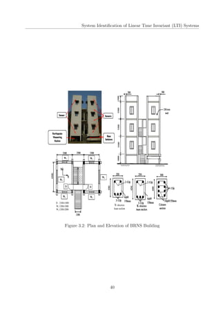
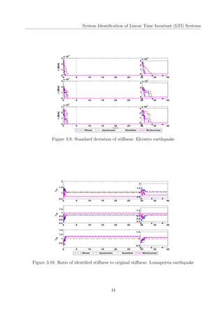
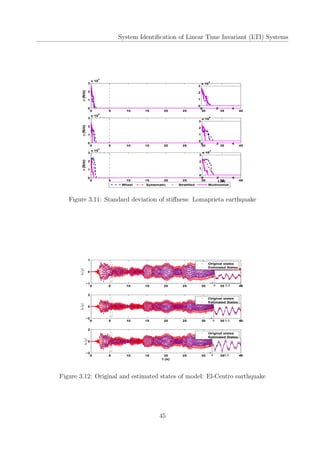
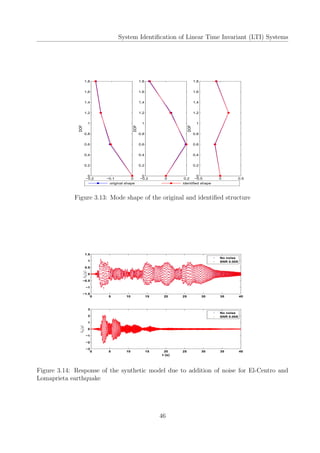
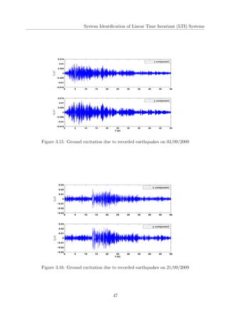
This document is a project report submitted for the degree of Bachelor of Technology in Civil Engineering at IIT Guwahati. It investigates using sequential Markov Chain Monte Carlo (MCMC) simulation based algorithms, also known as particle filters, for parameter estimation of linear time-invariant (LTI) structural systems subjected to non-stationary earthquake excitations. The report describes implementing Sequential Importance Sampling (SIS), Sequential Importance Resampling (SIR), and Bootstrap filters to identify stiffness and damping parameters of a 3-story shear building model and a multi-story reinforced concrete framed building (BRNS building) at IIT Guwahati. It compares the performance of these filters based on identified natural frequencies and