Download to read offline

![numPart = 5; % number of particles
numVar =3; % Number of variables
fileName = 'objfunc';
w = 0.5; % Inertia weight
C1 = 2; % learning factor for local search
C2 = 2; % learning factor for local search
maxGen =500; % Maximum generation
lb = 50; % Lower bound of the variables
ub = 180; % Upper bound of the variables
X = lb + (ub-lb)*rand(numPart,numVar); % initialize X
V = lb + (ub-lb)*rand(numPart,numVar); % initialize V
for i=1:numPart
% f(i)=fitness(X(i,:));
f(i)=feval(fileName,X(i,:));
end
X = [V X f'];
Y = sortrows(X,2*numVar+1);
pbest = Y;
gbest = Y(1,:);
for gen=1:maxGen % generation loop
for part=1:numPart % Particle loop
for dim=1:numVar % Variable loop
V(part,dim)=w*V(part,dim)+C1*rand(1,1)*(pbest(part,numVar+dim)-
X(part,numVar+dim))+C2*rand(1,1)*(gbest(numVar+dim)-X(part,numVar+dim));
X(part,numVar+dim)=X(part,numVar+dim)+V(part,dim);
end
while(X(part,numVar + 1)< 0 || X(part,numVar + 2)< 0 || X(part,numVar
+ 3)<0 || X(part,numVar + 1) - 50 <= 0 || X(part,numVar + 1) + X(part,numVar
+ 2)-100 <= 0 || X(part,numVar + 1) + X(part,numVar + 2) + X(part,numVar +
3) -150 <=0)
for dim=1:numVar % Variable loop
V(part,dim)=w*V(part,dim)+C1*rand(1,1)*(pbest(part,numVar+dim)-
X(part,numVar+dim))+C2*rand(1,1)*(gbest(numVar+dim)-X(part,numVar+dim));
X(part,numVar+dim)=X(part,numVar+dim)+V(part,dim);
end
end
%
% fnew = fitness(X(part,numVar+1:numVar+dim));
fnew = feval(fileName,X(part,numVar+1:numVar+dim));
X(part,2*numVar+1)=fnew;
if (fnew<X(part,2*numVar+1))
pbest(part,:)=X(part,:);
end
end](https://image.slidesharecdn.com/optimization-151206044457-lva1-app6892/85/Optimization-5-320.jpg)
![Y = sortrows(X,2*numVar+1);
if (Y(1,2*numVar+1)<gbest(2*numVar+1))
gbest=Y(1,:);
end
first_var(gen) = gbest(4);
second_var(gen) = gbest(5);
third_var(gen) = gbest(6);
obj_value(gen,p) = gbest(7);
disp(['Generation ', num2str(gen)]);
disp(['Best Value ', num2str(gbest(numVar+1:2*numVar+1))]);
end
numPart = numPart + 15;
end
generations = 1:500;
% subplot(2,2,1)
% plot(generations,obj_value(:,1))
% hold on
% subplot(2,2,2)
% plot(generations,obj_value(:,2))
% hold on
% subplot(2,2,3)
% plot(generations,obj_value(:,3))
% hold on
% subplot(2,2,4)
% plot(generations,obj_value(:,4))
plot(generations,obj_value(:,1),'b',generations,obj_value(:,2),'g',generation
s,obj_value(:,3),'k',generations,obj_value(:,4),'r')
cpu_time = cputime-tm ;
The modified part has been highlighted above and based on the above code some
of the results were plotted which are shown as:](https://image.slidesharecdn.com/optimization-151206044457-lva1-app6892/85/Optimization-6-320.jpg)
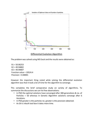

The document presents a comparative study of genetic algorithms (GA) and particle swarm algorithms (PSO) for optimizing production costs in a manufacturing firm supplying refrigerators. The analysis includes problem constraints, objective functions, and methods used, revealing that the GA achieved a cost function value of 10504.8 after 6 iterations, while PSO converged to its optimal solution after 300 generations. Observations note that while GA yields better results in terms of cost efficiency, it is generally quicker than PSO, and increasing particle numbers in PSO improves precision but requires more computational time.