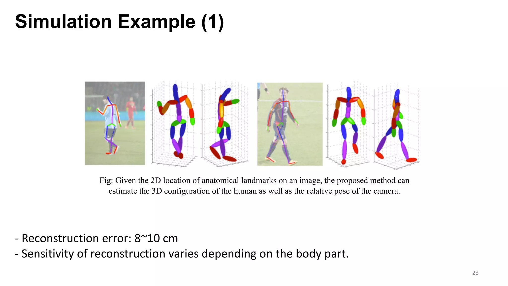
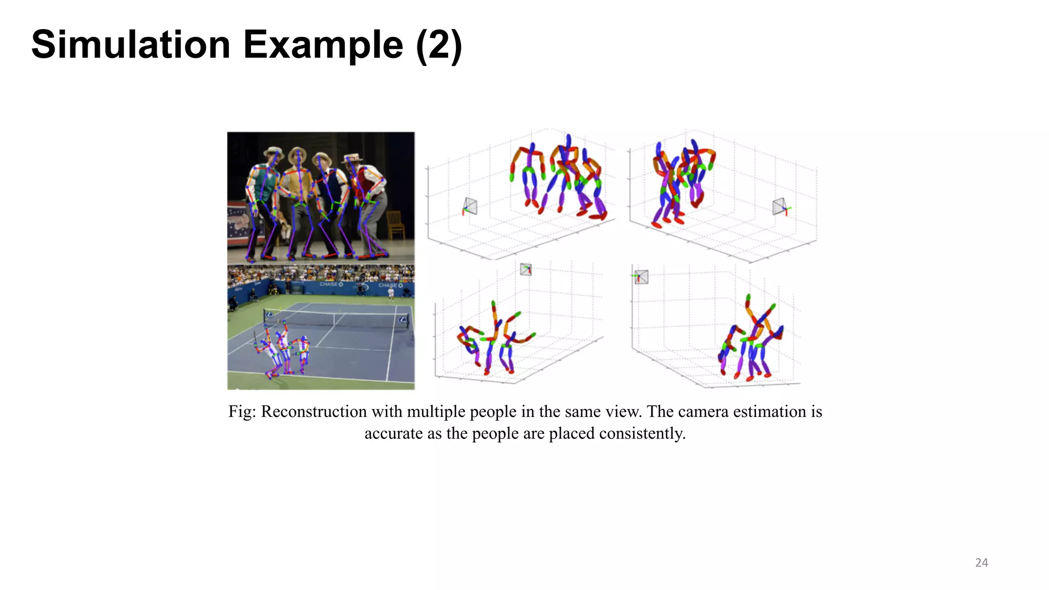
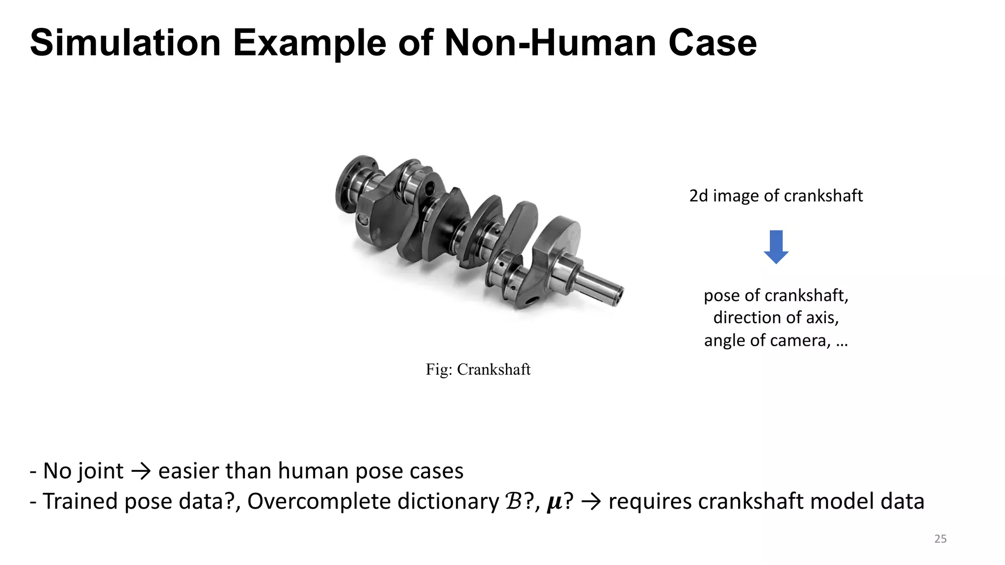
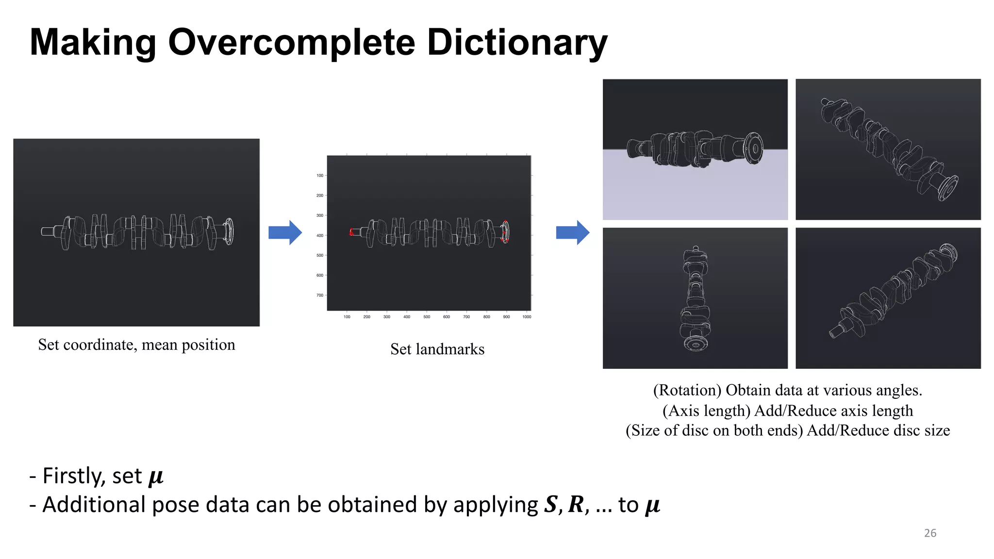
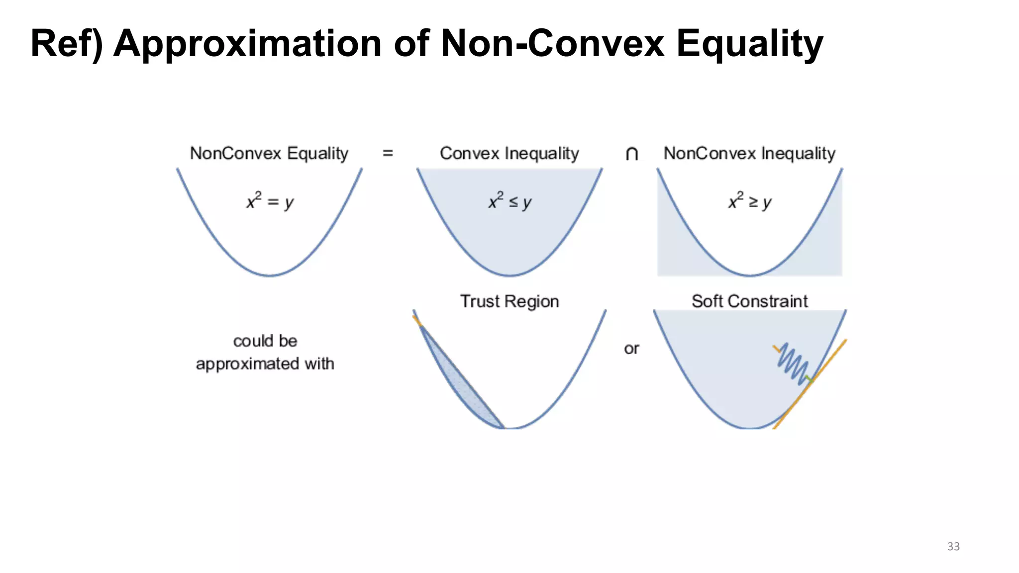
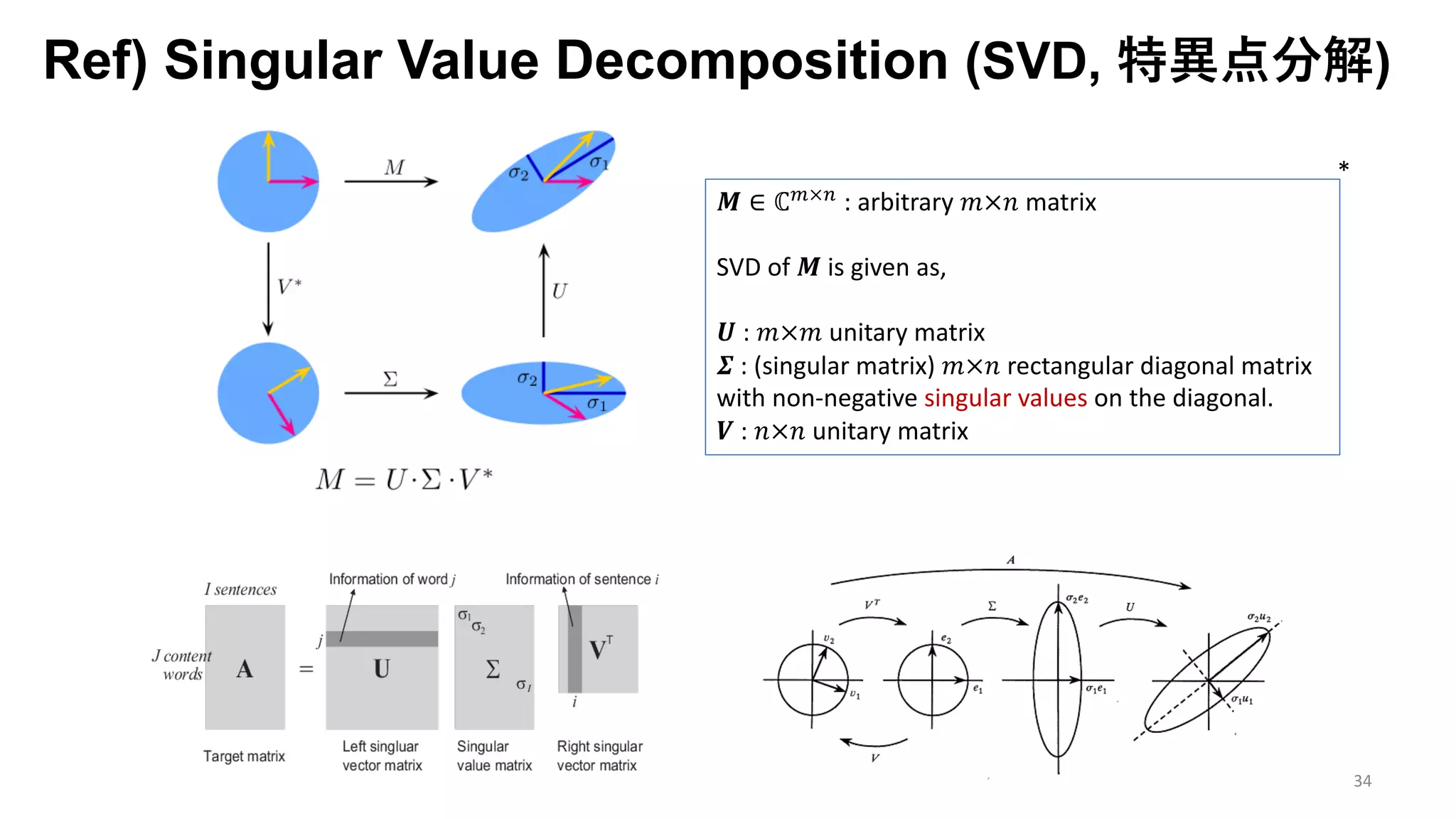
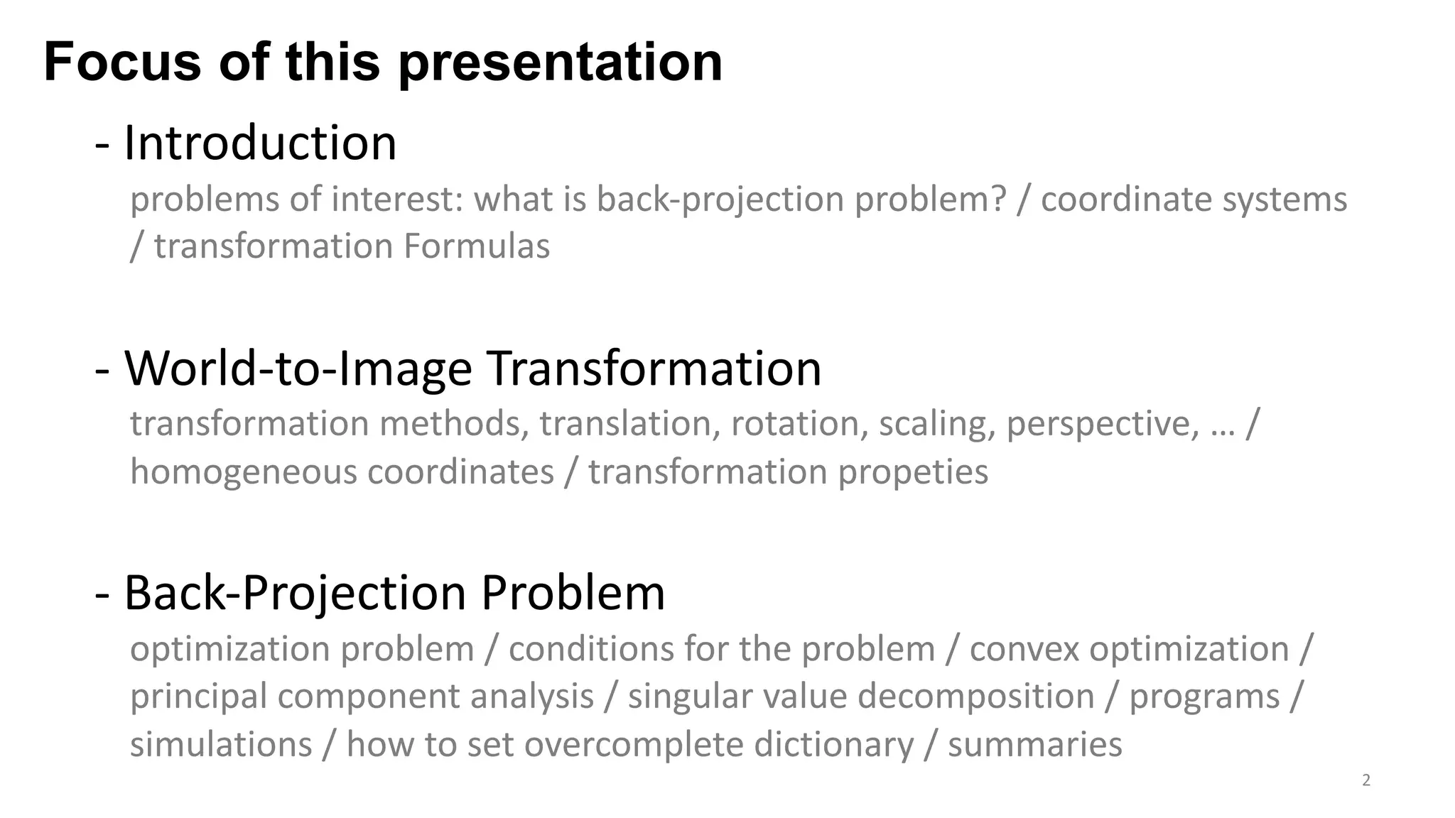
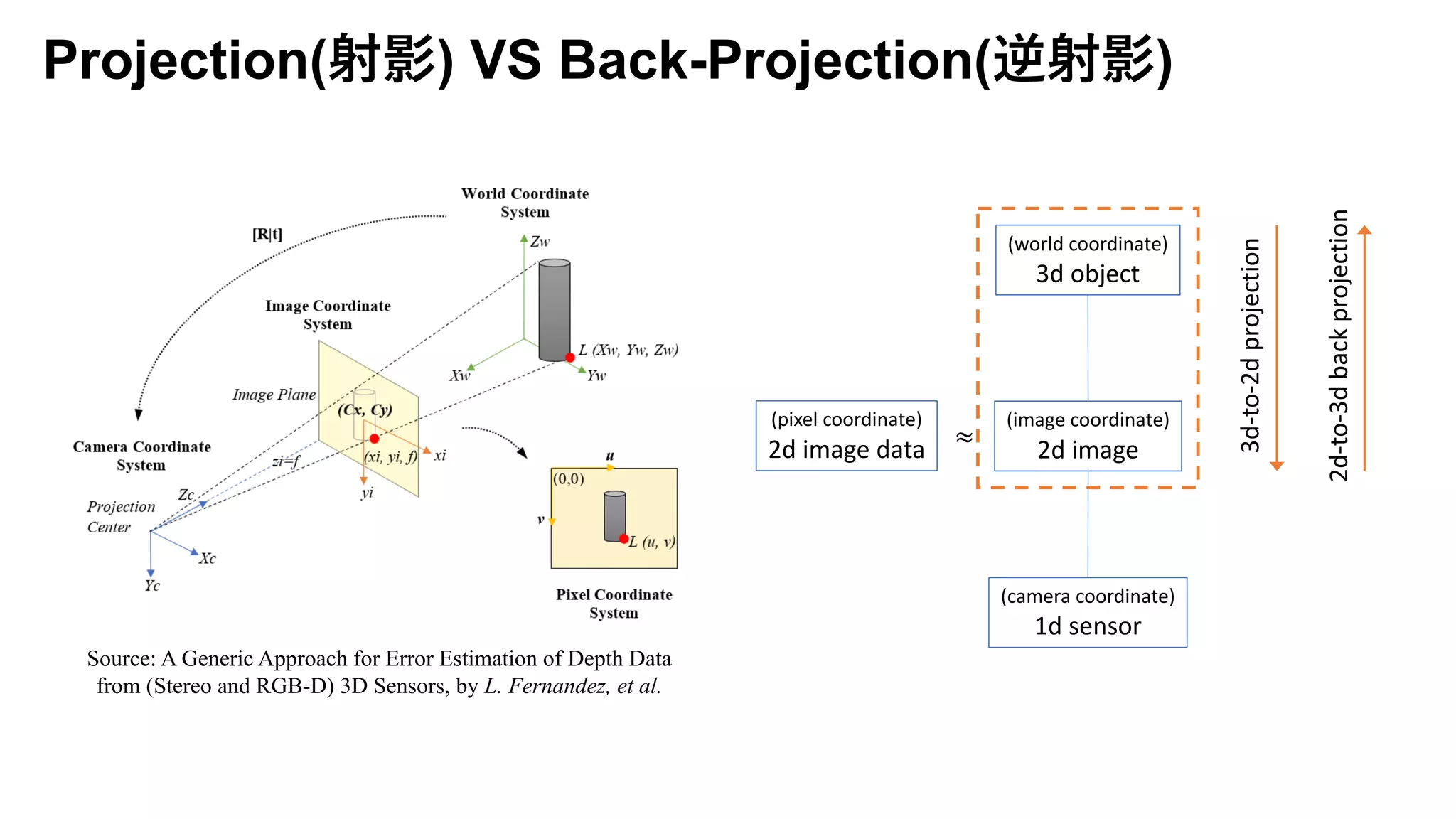
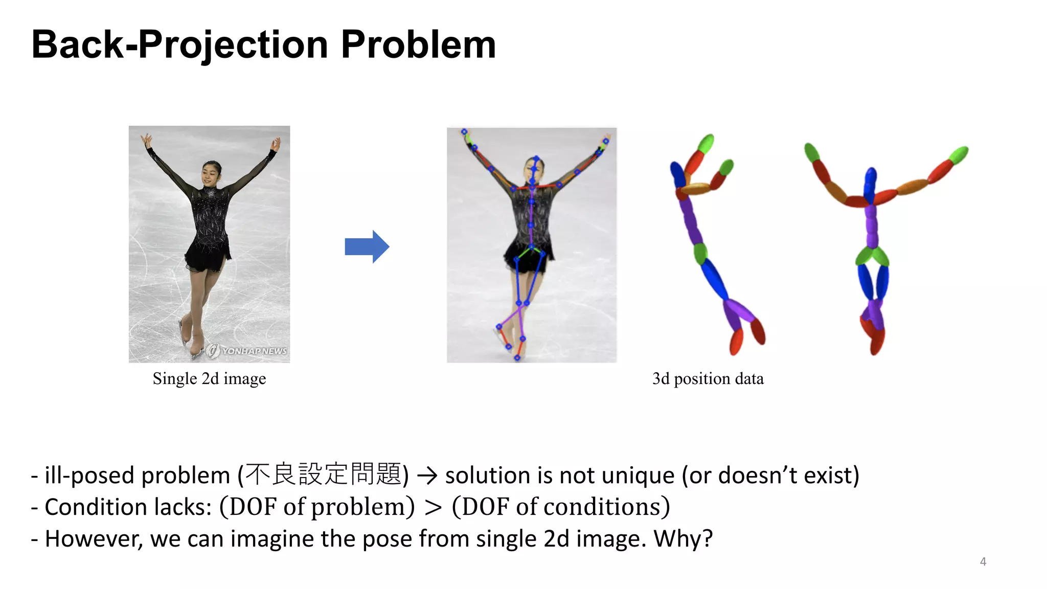
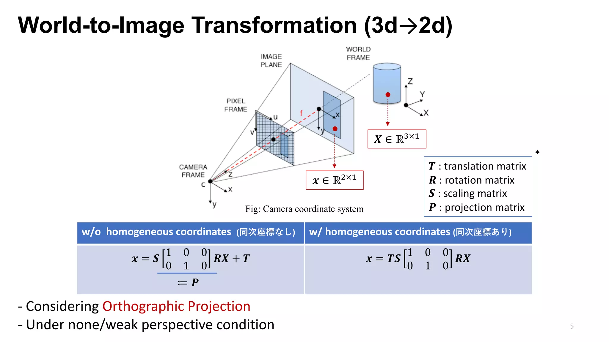
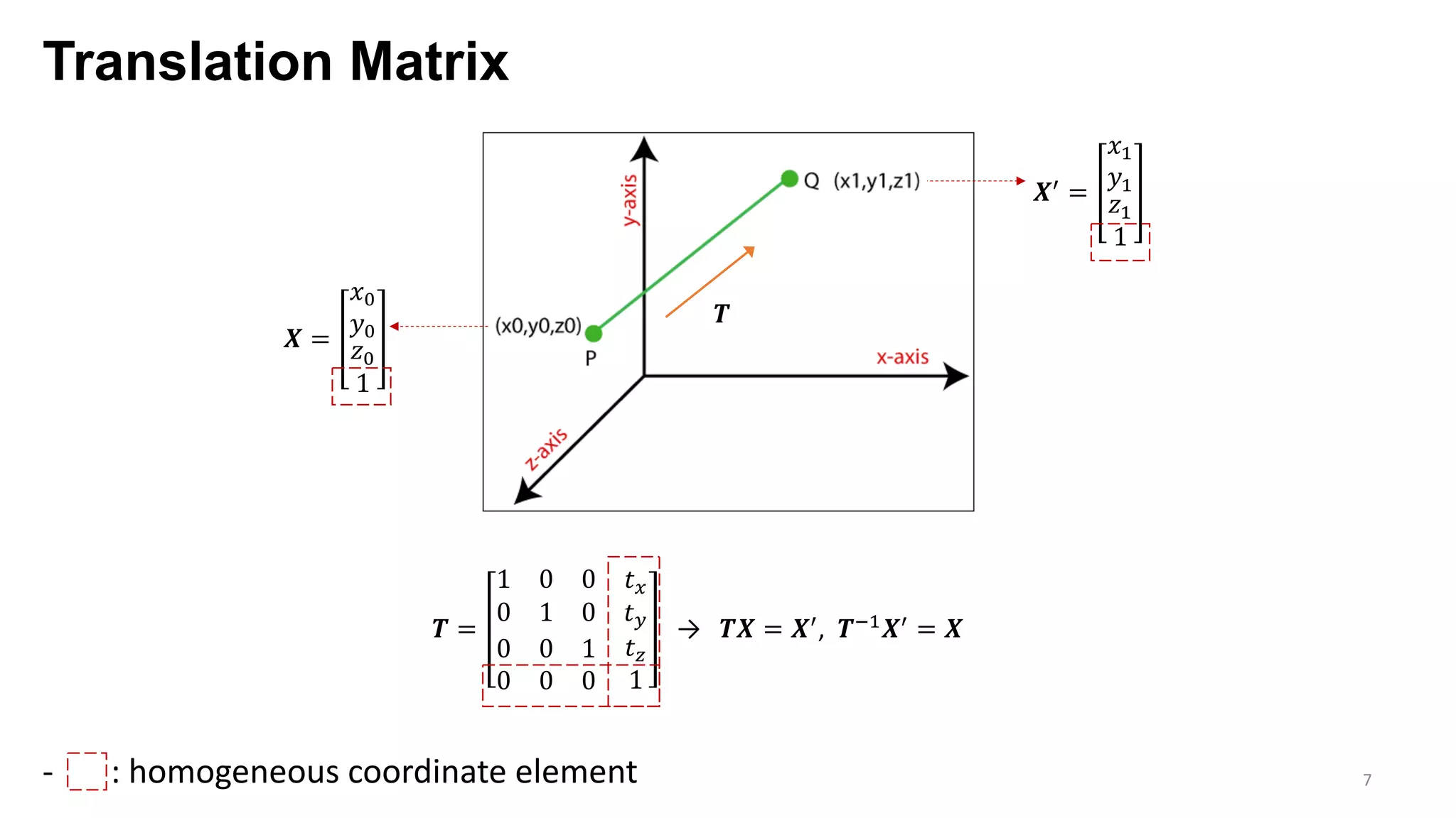
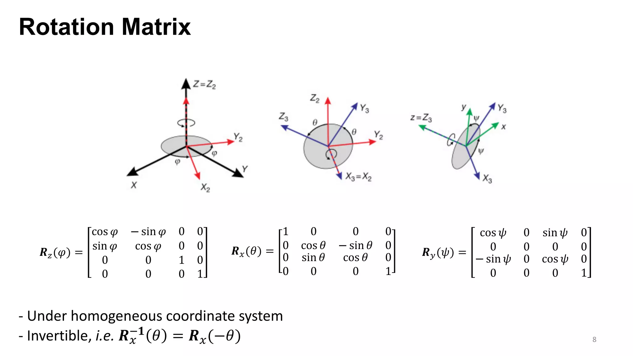
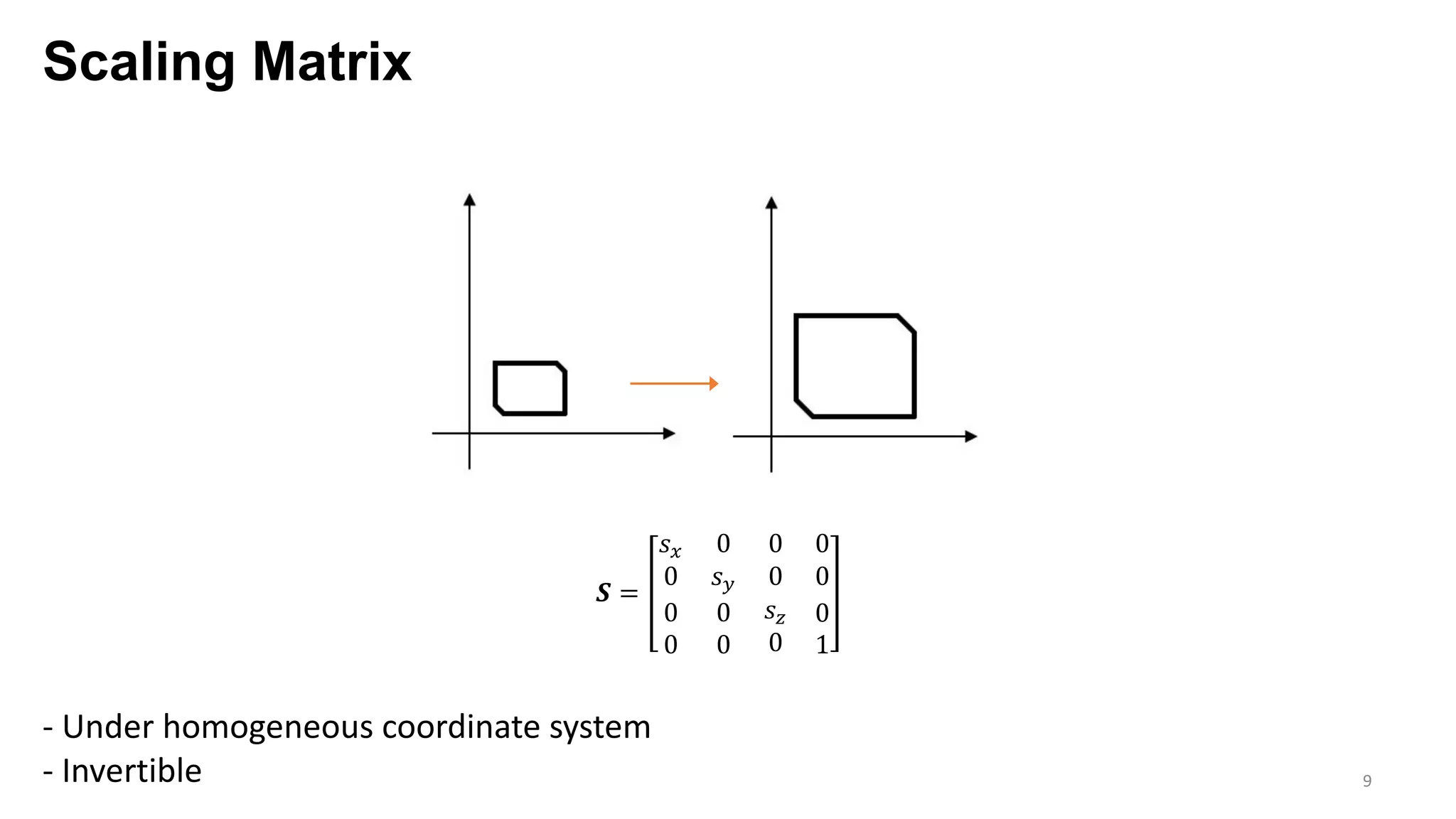
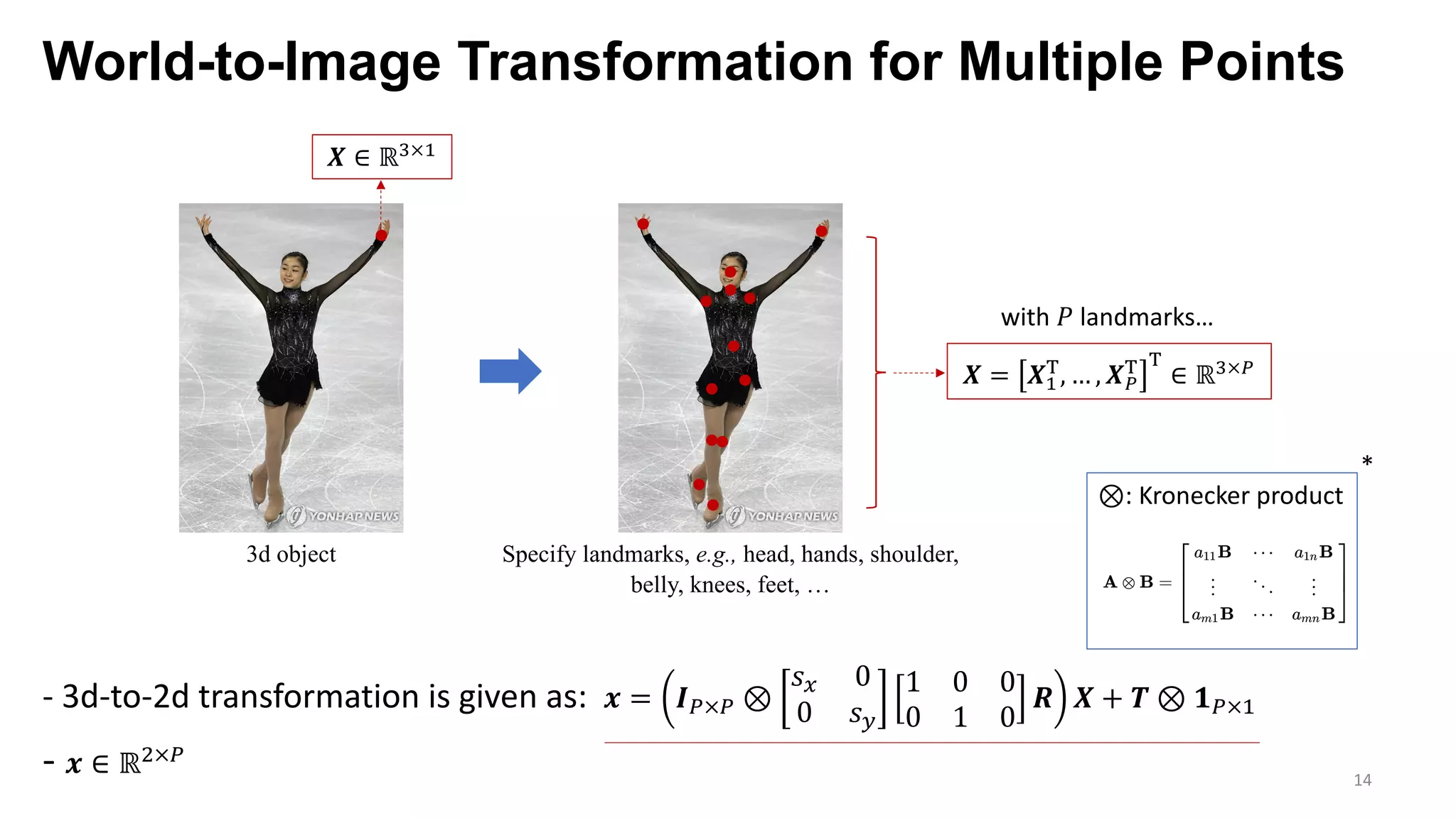
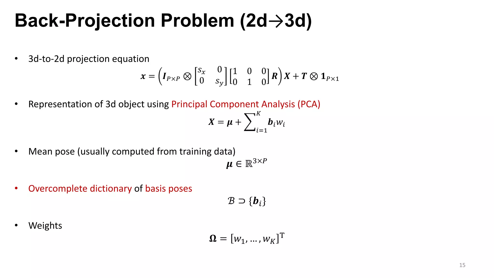
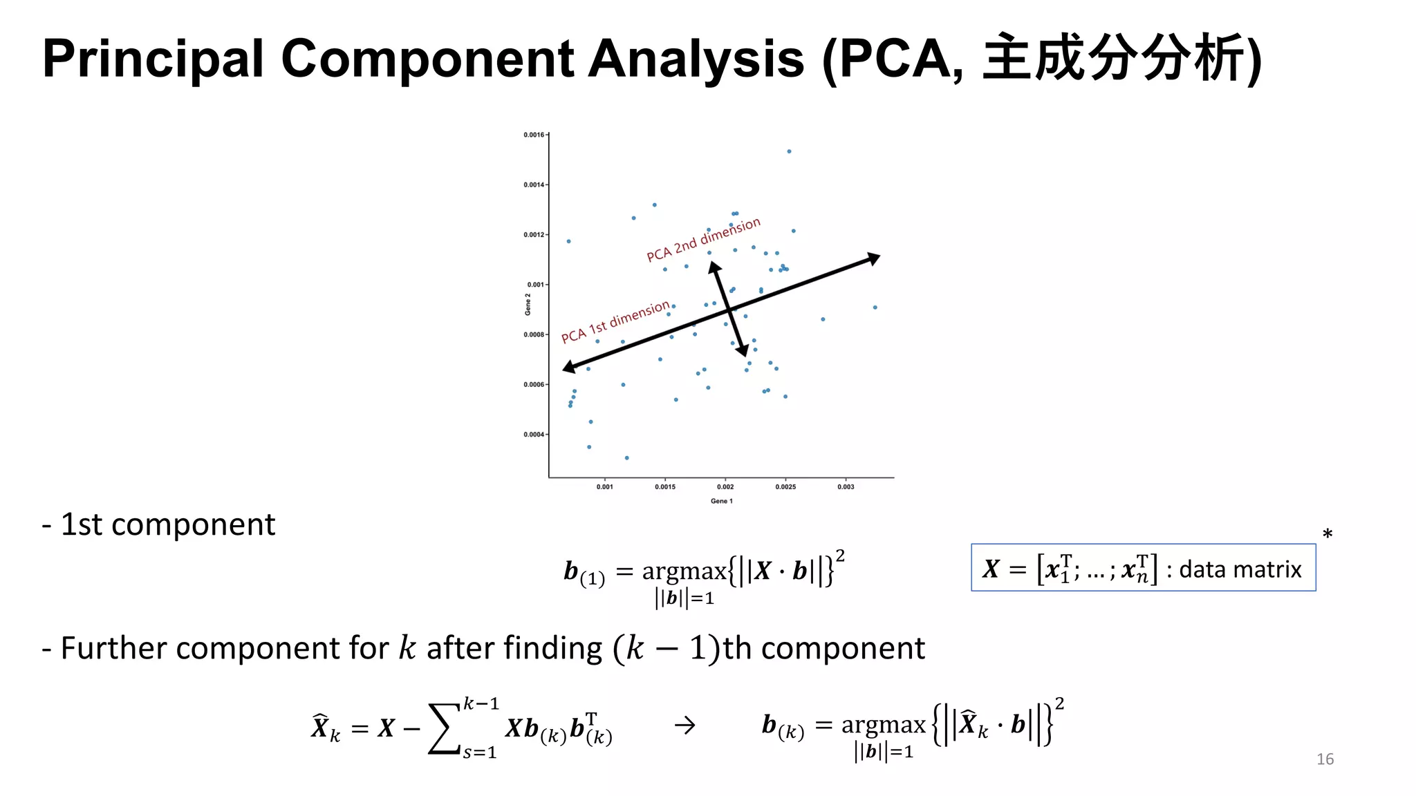
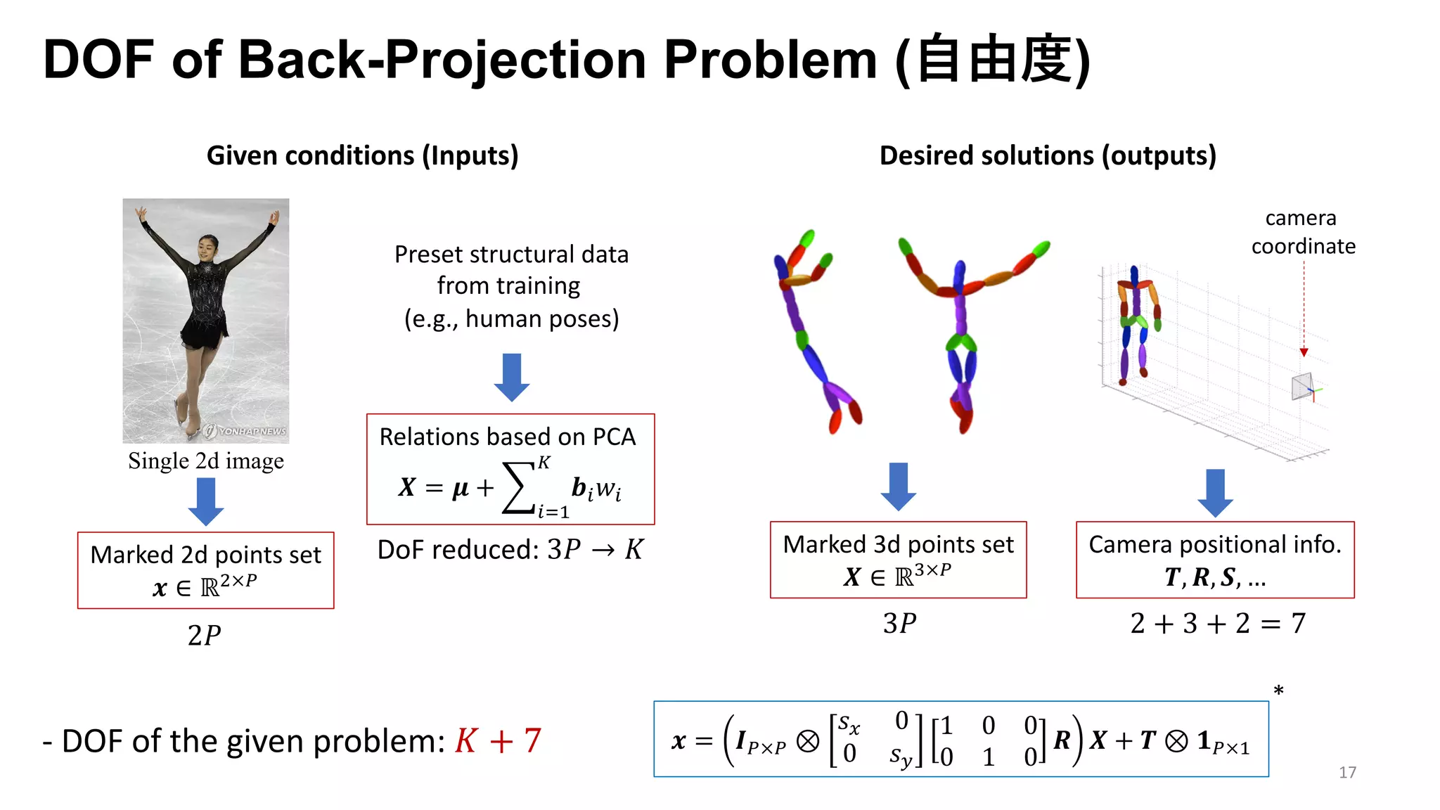
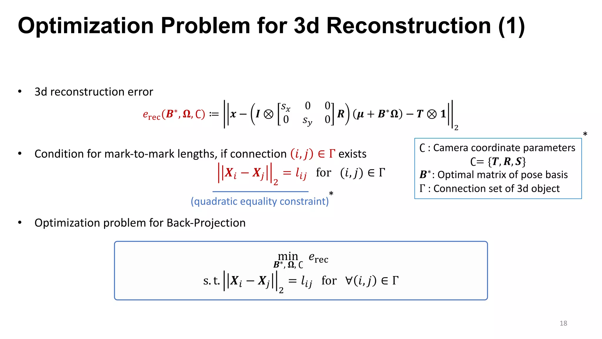
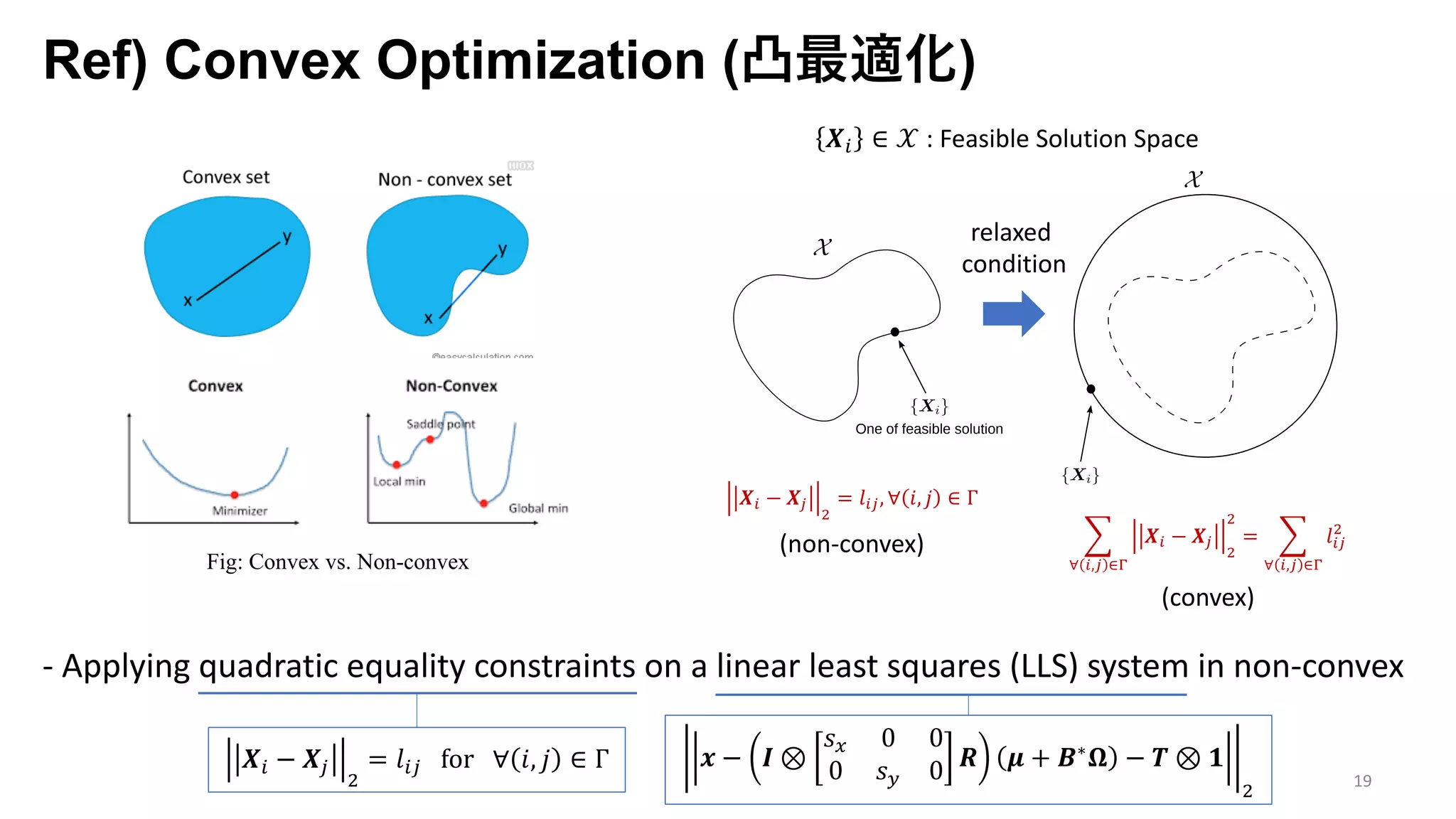
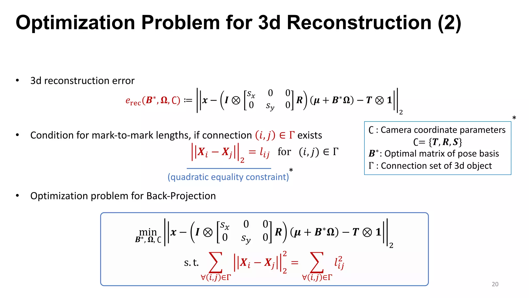
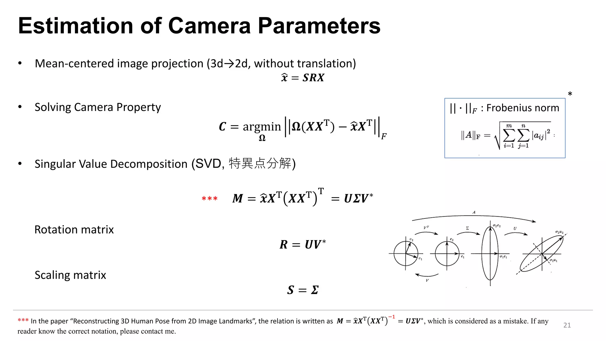
The document presents an exploration of the 2D-to-3D back-projection problem, focusing on various transformation methods and the optimization necessary for reconstructing 3D human poses from 2D image landmarks. Technical topics include world-to-image transformations, principal component analysis, and convex optimization, along with practical simulations demonstrating effectiveness. Theoretical foundations and potential applications are highlighted, alongside references to supporting literature and resources.

1. 1
Inspired by open-source paper, “Reconstructing 3D Human Pose from 2D Image Landmarks,”
by V. Ramakrishna, T. Kanade, and Y. Sheikh (ECCV 2012: Computer Vision – ECCV 2012 pp. 573-586)
Seongcheol Baek
PhD Course, Graduate School of Engineering,
Hikihara Lab: Laboratory of Advanced Electrical Systems Theory,
Kyoto University
Email: s-baek@dove.kuee.kyoto-u.ac.jp
2020/03/27
Theories and Engineering Technics of
2D-to-3D Back-Projection Problem

2. Focus of this presentation
- Introduction
problems of interest: what is back-projection problem? / coordinate systems
/ transformation Formulas
- World-to-Image Transformation
transformation methods, translation, rotation, scaling, perspective, … /
homogeneous coordinates / transformation propeties
- Back-Projection Problem
optimization problem / conditions for the problem / convex optimization /
principal component analysis / singular value decomposition / programs /
simulations / how to set overcomplete dictionary / summaries
2

3. Source: A Generic Approach for Error Estimation of Depth Data
from (Stereo and RGB-D) 3D Sensors, by L. Fernandez, et al.
Projection(射影) VS Back-Projection(逆射影)
(world coordinate)
3d object
(image coordinate)
2d image
(camera coordinate)
1d sensor
(pixel coordinate)
2d image data ≈
3d-to-2dprojection
2d-to-3dbackprojection

4. Back-Projection Problem
4
- ill-posed problem (不良設定問題) → solution is not unique (or doesn’t exist)
- Condition lacks: DOF of problem > DOF of conditions
- However, we can imagine the pose from single 2d image. Why?
Single 2d image 3d position data

5. World-to-Image Transformation (3d→2d)
5
𝒙 ∈ ℝ7×9
𝑿 ∈ ℝ;×9
Fig: Camera coordinate system
- Considering Orthographic Projection
- Under none/weak perspective condition
w/o homogeneous coordinates (同次座標なし) w/ homogeneous coordinates (同次座標あり)
𝒙 = 𝑺
1 0 0
0 1 0
𝑹𝑿 + 𝑻 𝒙 = 𝑻𝑺
1 0 0
0 1 0
𝑹𝑿
≔ 𝑷
𝑻 : translation matrix
𝑹 : rotation matrix
𝑺 : scaling matrix
𝑷 : projection matrix
*

6. Homogeneous Coordinate (同次座標系)
6
Fig: Polynomial curve defined in homogeneous coordinates (blue)
and its projection on plane – rational curve (red)
- Coordinate system that represents an n-dimensional projective space with n+1 coordinates
- Merits: simple and symmetric formulations

7. Translation Matrix
7
𝑻 =
1 0 0 𝑡F
0 1 0 𝑡G
0
0
0
0
1
0
𝑡H
1
→ 𝑻𝑿 = 𝑿I, 𝑻J9 𝑿I = 𝑿
𝑿 =
𝑥L
𝑦L
𝑧L
1
𝑿I =
𝑥9
𝑦9
𝑧9
1
𝑻
- : homogeneous coordinate element

8. Rotation Matrix
8
𝑹H(𝜑) =
cos 𝜑 − sin 𝜑 0 0
sin 𝜑 cos 𝜑 0 0
0
0
0
0
1
0
0
1
𝑹F(𝜃) =
1 0 0 0
0 cos 𝜃 − sin 𝜃 0
0
0
sin 𝜃
0
cos 𝜃
0
0
1
𝑹G(𝜓) =
cos 𝜓 0 sin 𝜓 0
0 0 0 0
− sin 𝜓
0
0
0
cos 𝜓
0
0
1
- Under homogeneous coordinate system
- Invertible, i.e. 𝑹F
J𝟏 𝜃 = 𝑹F(−𝜃)

9. Scaling Matrix
9
𝑺 =
𝑠F 0 0 0
0 𝑠G 0 0
0
0
0
0
𝑠H
0
0
1
- Under homogeneous coordinate system
- Invertible

10. Reflection, Skew, …
10
(=skew)
𝑺𝑯 =
1 𝑎F
G
𝑎F
H 0
𝑎G
F
1 𝑎G
H
0
𝑎H
F
0
𝑎H
G
0
1
0
0
1
𝑹𝑭FG =
1 0 0 0
0 1 0 0
0
0
0
0
−1
0
0
1

11. Ref) Perspective Transformation (3d→2d, 透視変換)
11
Perspective
projection
Orthogonal
projection
:Vanishing points
*
Fig: One-point perspective drawing of a
column of cubes
Fig: Relation between perspective
projection and orthogonal projection
image plane
𝑥I
=
Z[
[
𝑥, 𝑦′ =
Z[
[
𝑦
without considering rotation
camera coordinate
focal
length
object in
world
coordinate
𝑑F
𝑑G
𝑑H
= 𝑹F(𝜃F)𝑹G(𝜃G) 𝑹H 𝜃H
𝑎F
𝑎G
𝑎H
−
𝑐F
𝑐G
𝑐H
Object position with respect to Camera Coordinate
object camera
𝑏F =
𝑒H
𝑑H
𝑑F + 𝑒F
Perspective projection from 3d to 2d
𝑏G =
𝑒H
𝑑H
𝑑G + 𝑒G
(𝑒F, 𝑒G, 𝑒H): position of image plane
*

12. Properties of Transformation Matrices
12
- In general, the matrix multiplication is not commutative (交換法則X)
- i.e., 𝑴9 𝑴7 ≠ 𝑴7 𝑴9 in usual cases
𝑻𝑻I ≠ 𝑻I 𝑻

13. Ref) World-to-Image Transformation (3d→2d)
13
𝒙 ∈ ℝ7×9
𝑿 ∈ ℝ;×9
Fig: Camera coordinate system
𝑻 : translation matrix
𝑹 : rotation matrix
𝑺 : scaling matrix
𝑷 : projection matrix
*
𝒙 = 𝑻𝑺
1 0 0
0 1 0
𝑹𝑿 (with homogeneous coordinates)
- In orthogonal coordinate manner,
𝒙 =
𝑠F 0 0
0 𝑠G 0 𝑹𝑿 +
𝑡F
𝑡G
⋯ 𝑿 = 𝑋9, 𝑋7, 𝑋;, 1 g
⋯ 𝑿 = 𝑋9, 𝑋7, 𝑋;
g

14. World-to-Image Transformation for Multiple Points
14
3d object Specify landmarks, e.g., head, hands, shoulder,
belly, knees, feet, …
𝑿 ∈ ℝ;×9
𝑿 = 𝑿9
h
, … , 𝑿j
h h
∈ ℝ;×j
- 3d-to-2d transformation is given as: 𝒙 = 𝑰j×j ⊗
𝑠F 0
0 𝑠G
1 0 0
0 1 0
𝑹 𝑿 + 𝑻 ⊗ 𝟏j×9
- 𝒙 ∈ ℝ7×j
with 𝑃 landmarks…
⊗: Kronecker product
*

15. Back-Projection Problem (2d→3d)
15
• 3d-to-2d projection equation
𝒙 = 𝑰j×j ⊗
𝑠F 0
0 𝑠G
1 0 0
0 1 0
𝑹 𝑿 + 𝑻 ⊗ 𝟏j×9
• Representation of 3d object using Principal Component Analysis (PCA)
𝑿 = 𝝁 + o
pq9
r
𝒃p 𝑤p
• Mean pose (usually computed from training data)
𝝁 ∈ ℝ;×j
• Overcomplete dictionary of basis poses
ℬ ⊃ {𝒃p}
• Weights
𝛀 = 𝑤9, … , 𝑤r
h

16. Principal Component Analysis (PCA, 主成分分析)
16
- 1st component
𝒃(9) = argmax
𝒃 q9
𝑿 } 𝒃
7
- Further component for 𝑘 after finding (𝑘 − 1)th component
𝑿 = 𝒙9
h
; … ; 𝒙€
h
: data matrix
*
𝒃(•) = argmax
𝒃 q9
‚𝑿• } 𝒃
7
‚𝑿• = 𝑿 − o
ƒq9
•J9
𝑿𝒃(•) 𝒃 •
h →

17. DOF of Back-Projection Problem (⾃由度)
17
Given conditions (Inputs)
Single 2d image
Marked 2d points set
𝒙 ∈ ℝ7×j
Relations based on PCA
𝑿 = 𝝁 + o
pq9
r
𝒃p 𝑤p
Preset structural data
from training
(e.g., human poses)
Desired solutions (outputs)
Marked 3d points set
𝑿 ∈ ℝ;×j
camera
coordinate
Camera positional info.
𝑻, 𝑹, 𝑺, …
𝒙 = 𝑰j×j ⊗
𝑠F 0
0 𝑠G
1 0 0
0 1 0
𝑹 𝑿 + 𝑻 ⊗ 𝟏j×9
*
3𝑃 2 + 3 + 2 = 72𝑃
DoF reduced: 3𝑃 → 𝐾
- DOF of the given problem: 𝐾 + 7

18. Optimization Problem for 3d Reconstruction (1)
18
• 3d reconstruction error
𝑒‰Š‹(𝑩∗, 𝛀, ∁) ≔ 𝒙 − 𝑰 ⊗
𝑠F 0 0
0 𝑠G 0 𝑹 𝝁 + 𝑩∗ 𝛀 − 𝑻 ⊗ 𝟏
7
• Condition for mark-to-mark lengths, if connection 𝑖, 𝑗 ∈ Γ exists
𝑿p − 𝑿’
7
= 𝑙p’ for (𝑖, 𝑗) ∈ Γ
• Optimization problem for Back-Projection
∁ : Camera coordinate parameters
∁= {𝑻, 𝑹, 𝑺}
𝑩∗: Optimal matrix of pose basis
Γ : Connection set of 3d object
*
min
𝑩∗, 𝛀, ∁
𝑒‰Š‹
s. t. 𝑿p − 𝑿’
7
= 𝑙p’ for ∀ 𝑖, 𝑗 ∈ Γ
*
(quadratic equality constraint)

19. Ref) Convex Optimization (凸最適化)
19
Fig: Convex vs. Non-convex
- Applying quadratic equality constraints on a linear least squares (LLS) system in non-convex
𝒙 − 𝑰 ⊗
𝑠F 0 0
0 𝑠G 0 𝑹 𝝁 + 𝑩∗ 𝛀 − 𝑻 ⊗ 𝟏
7
𝑿p − 𝑿’
7
= 𝑙p’ for ∀ 𝑖, 𝑗 ∈ Γ
𝑿p ∈ 𝒳 : Feasible Solution Space
One of feasible solution
𝑿p − 𝑿’
7
= 𝑙p’, ∀ 𝑖, 𝑗 ∈ Γ
o
∀ p,’ ∈—
𝑿p − 𝑿’
7
7
= o
∀ p,’ ∈—
𝑙p’
7
relaxed
condition
(non-convex)
(convex)

20. Optimization Problem for 3d Reconstruction (2)
20
• 3d reconstruction error
𝑒‰Š‹(𝑩∗, 𝛀, ∁) ≔ 𝒙 − 𝑰 ⊗
𝑠F 0 0
0 𝑠G 0 𝑹 𝝁 + 𝑩∗ 𝛀 − 𝑻 ⊗ 𝟏
7
• Condition for mark-to-mark lengths, if connection 𝑖, 𝑗 ∈ Γ exists
𝑿p − 𝑿’
7
= 𝑙p’ for (𝑖, 𝑗) ∈ Γ
• Optimization problem for Back-Projection
∁ : Camera coordinate parameters
∁= {𝑻, 𝑹, 𝑺}
𝑩∗: Optimal matrix of pose basis
Γ : Connection set of 3d object
*
min
𝑩∗, 𝛀, ∁
𝒙 − 𝑰 ⊗
𝑠F 0 0
0 𝑠G 0 𝑹 𝝁 + 𝑩∗ 𝛀 − 𝑻 ⊗ 𝟏
7
s. t. o
∀ p,’ ∈—
𝑿p − 𝑿’
7
7
= o
∀ p,’ ∈—
𝑙p’
7
*
(quadratic equality constraint)

21. Estimation of Camera Parameters
21
• Mean-centered image projection (3d→2d, without translation)
˜𝒙 = 𝑺𝑹𝑿
• Solving Camera Property
𝑪 = argmin
𝛀
𝛀(𝑿𝑿h) − ˜𝒙 𝑿h
š
• Singular Value Decomposition (SVD, 特異点分解)
𝑴 = ˜𝒙 𝑿h 𝑿𝑿h h
= 𝑼𝜮𝑽∗
Rotation matrix
𝑹 = 𝑼𝑽∗
Scaling matrix
𝑺 = 𝜮
|| } ||š : Frobenius norm
*
*** In the paper “Reconstructing 3D Human Pose from 2D Image Landmarks”, the relation is written as 𝑴 = ˜𝒙 𝑿h 𝑿𝑿h J9
= 𝑼𝜮𝑽∗, which is considered as a mistake. If any
reader know the correct notation, please contact me.
***

22. Program to Solve Back-Projection Problem
22
(1) Initialization
𝒓L = 𝒙 − 𝑰 ⊗ 𝑺𝑹 𝝁 − 𝑻 ⊗ 𝟏
(2) If 𝒓 < (tol), proceed to (8)
(3) 𝑖¢£¤ = argmax
p
𝒓 , 𝑰 ⊗ 𝑺𝑹 𝑩p
(4) 𝑩∗ ← [𝑩∗ 𝑩p§¨©
]
(5) Solve:
argmin
𝛀, ∁
˜𝒙 − 𝑰 ⊗ 𝑺𝑹 𝑩∗ 𝛀 7
(under the mark-to-mark length conditions)
(6) Recompute:
𝒓 «9 = 𝒙 − 𝑰 ⊗ 𝒔𝑹 (𝝁 + 𝑩∗ 𝛀∗) − 𝑻 ⊗ 𝟏
(7) Set:
𝛀 «9 ← 𝛀∗
(8) Return:
{𝑩∗, 𝛀∗, ∁}

23. Simulation Example (1)
23
- Reconstruction error: 8~10 cm
- Sensitivity of reconstruction varies depending on the body part.
Fig: Given the 2D location of anatomical landmarks on an image, the proposed method can
estimate the 3D configuration of the human as well as the relative pose of the camera.

24. Simulation Example (2)
24
Fig: Reconstruction with multiple people in the same view. The camera estimation is
accurate as the people are placed consistently.

25. Simulation Example of Non-Human Case
25
Fig: Crankshaft
- No joint → easier than human pose cases
- Trained pose data?, Overcomplete dictionary ℬ?, 𝝁? → requires crankshaft model data
2d image of crankshaft
pose of crankshaft,
direction of axis,
angle of camera, …

26. Making Overcomplete Dictionary
26
Set coordinate, mean position Set landmarks
(Rotation) Obtain data at various angles.
(Axis length) Add/Reduce axis length
(Size of disc on both ends) Add/Reduce disc size
- Firstly, set 𝝁
- Additional pose data can be obtained by applying 𝑺, 𝑹, … to 𝝁

27. Simulation Example (3)
27
2dimageinput3dposedataoutput

28. Summaries
28
- 2d-to-3d back-projection problem was discussed
- World-to-image transformation was studied, and employed in the problem formulation
- Optimization problem to seek 3d landmarks was established, along with the detailed
reasoning for the given condition (mark-to-mark lengths)
- Some simulations were examined, including human pose case and non-human pose case
Also discussed...
Theoretical technics such as principal component analysis, convex optimization, singular
value decomposition, orthogonal Procrustes problem, etc.

29. 29
Thank you!
- Source code for simulations
Official implementation of " Reconstructing 3D Human Pose from 2D Image Landmarks " (Github) ... https://github.com/varunnr/camera_and_pose
- This presentation is also available on:
https://www.slideshare.net/SeongcheolBaek/theories-and-engineering-technics-of-2dto3d-backprojection-problem

30. References
30
- Crux of Presentation
V. Ramakrishna, et al., Reconstructing 3D Human Pose from 2D Image Landmarks (ECCV 2012: Computer Vision – ECCV 2012 pp. 573-586) …
https://www.researchgate.net/publication/262170821_Reconstructing_3D_Human_Pose_from_2D_Image_Landmarks
- World-to-Image Transformation
Camera Coordinate Systems … http://people.bu.edu/chenyua/CS585finalproject/CS585_Project_Report.html
Homogeneous Coordinates (Wikipedia) … https://en.wikipedia.org/wiki/Homogeneous_coordinates
Computer Graphics Transformations (Lecture Note by D. Breen, et al.) … https://www.cs.drexel.edu/~david/Classes/CS536/Lectures/L-18_Transformations.pdf
Quarternion (Lecture Note by D. Breen, et al.) … https://www.cs.drexel.edu/~david/Classes/CS536/Lectures/L-18_Transformations.pdf
- Back-Projection
Principal Component Analysis (Wikipedia) … https://en.wikipedia.org/wiki/Principal_component_analysis
Singular Value Decomposition (Wikipedia) … https://en.wikipedia.org/wiki/Singular_value_decomposition
Convex Optimization (Wikipedia) … https://en.wikipedia.org/wiki/Convex_optimization
Convex Optimization (Book, Cambridge University Press) … https://web.stanford.edu/~boyd/cvxbook/
- Refs
Well-Posed Problem (Wikipedia) … https://en.wikipedia.org/wiki/Well-posed_problem
Classification of some 3D projections (Wikipedia) … https://en.wikipedia.org/wiki/3D_projection
Perspective Projection (Wikipedia) … https://en.wikipedia.org/wiki/3D_projection
Perspective Projection (StackExchange) … https://math.stackexchange.com/questions/2337183/one-point-perspective-formula

31. Ref) Classification of some 3D projections
31

32. Ref) Gan-Based Back-Projection Method
32

33. Ref) Approximation of Non-Convex Equality
33

34. Ref) Singular Value Decomposition (SVD, 特異点分解)
34
𝑴 ∈ ℂ®×€ : arbitrary 𝑚×𝑛 matrix
SVD of 𝑴 is given as,
𝑼 : 𝑚×𝑚 unitary matrix
𝜮 : (singular matrix) 𝑚×𝑛 rectangular diagonal matrix
with non-negative singular values on the diagonal.
𝑽 : 𝑛×𝑛 unitary matrix
*

35. Ref) Orthogonal Procrustes Problem through SVD
35
• Orthogonal Procrustes Problem:
Providing that two matrices 𝑨, 𝑩 are given, find an orthogonal matrix 𝑹 which most closely maps 𝑨 to 𝑩.
𝑹 = argmin
𝛀
𝛀𝐀 − 𝐁 š
⋯ (∗)
s. t. 𝛀h 𝛀 = 𝐈
• Solution using Singular Value Decomposition:
With two matrices 𝑨, 𝑩, it is considered that 𝑴 = 𝑩𝑨h is given. Here, assuming SVD of 𝑴 is given as below,
𝑴 = 𝑼𝜮𝑽∗,
then, the orthogonal matrix 𝑹 satisfying (∗) can be obtained as
𝑹 = 𝑼𝑽∗