이 문서는 신경망을 위한 새로운 학습 절차인 forward-forward 알고리즘을 소개하고, 이 방법이 몇 가지 작은 문제에서 충분히 잘 작동함을 보여줍니다. 이 알고리즘은 역전파의 정방향 및 역방향 패스를 대체하며, 양수(실제) 데이터와 음수 데이터 각각에 대해 정방향 패스를 수행하여 특정 목표를 달성합니다. 또한, FF 알고리즘의 잠재적 응용 분야와 향후 연구 방향에 대해 논의합니다.
Abstract
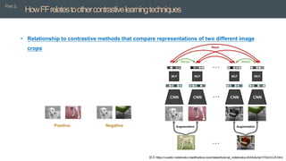
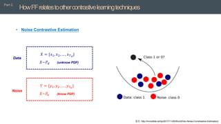
Part 1,
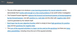
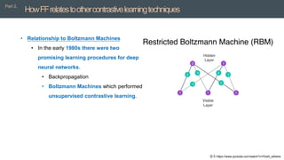
• Theaim of this paper is to introduce a new learning procedure for neural networks and to
demonstrate that it works well enough on a few small problems to be worth further investigation.
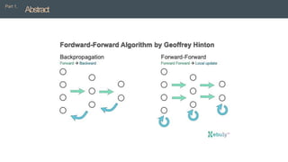
• The Forward-Forward algorithm replaces the forward and backward passes of backpropagation
by two forward passes, one with positive (i.e. real) data and the other with negative data which
could be generated by the network itself.
• Each layer has its own objective function which is simply to have high goodness for positive
data and low goodness for negative data.
• The sum of the squared activities in a layer can be used as the goodness but there are many
other possibilities, including minus the sum of the squared activities.
Whatiswrongwithbackpropagation
Part 3,
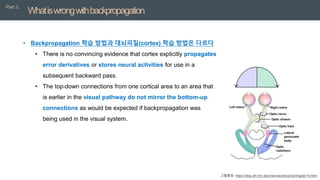
• Backpropagation학습 방법과 대뇌피질(cortex) 학습 방법은 다르다
• There is no convincing evidence that cortex explicitly propagates
error derivatives or stores neural activities for use in a
subsequent backward pass.
• The top-down connections from one cortical area to an area that
is earlier in the visual pathway do not mirror the bottom-up
connections as would be expected if backpropagation was
being used in the visual system.
그림참조: https://nba.uth.tmc.edu/neuroscience/s2/chapter15.html
24.
Whatiswrongwithbackpropagation
Part 3,
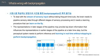
• 시퀀스를학습하는 방법으로 시간을 통한 backpropagation은 특히 불가능
• To deal with the stream of sensory input without taking frequent time-outs, the brain needs to
pipeline sensory data through different stages of sensory processing and it needs a learning
procedure that can learn on the fly.
• The representations in later stages of the pipeline may provide top-down information that
influences the representations in earlier stages of the pipeline at a later time step, but the
perceptual system needs to perform inference and learning in real time without stopping to
perform backpropagation.
그림참조: https://velog.io/@nkw011/seq-to-seq
25.
Whatiswrongwithbackpropagation
Part 3,
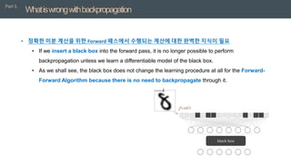
• 정확한미분 계산을 위한 Forward 패스에서 수행되는 계산에 대한 완벽한 지식이 필요
• If we insert a black box into the forward pass, it is no longer possible to perform
backpropagation unless we learn a differentiable model of the black box.
• As we shall see, the black box does not change the learning procedure at all for the Forward-
Forward Algorithm because there is no need to backpropagate through it.
26.
Whatiswrongwithbackpropagation
Part 3,
• FF알고리즘 장단점
• FF는 forward computation의 정확한 세부 사항을 알 수 없을 때도 사용가능
• Pipelining sequential data를 activity를 저장하거나 오류를 전파하기 위해 멈추지 않고 학습가능
• FF는 backpropagation에 비해서 다소 느리고 몇 가지 toy 문제에 대해 일반화가 잘 되지 않음
• 전력이 문제가 되지 않는 애플리케이션에 대한 backpropagation을 대체할 가능성은 낮음
• FF 알고리즘이 우수할 수 있는 두 가지 영역
• a model of learning in cortex
• a way of making use of very low-power analog hardware
TheForward-ForwardAlgorithm
Part 4,
• TheForward-Forward algorithm
• Greedy multi-layer learning procedure inspired by Boltzmann machines (Hinton and
Sejnowski, 1986)
• Noise Contrastive Estimation (Gutmann and Hyvärinen, 2010).
29.
TheForward-ForwardAlgorithm
Part 4,
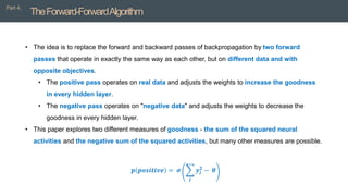
• Theidea is to replace the forward and backward passes of backpropagation by two forward
passes that operate in exactly the same way as each other, but on different data and with
opposite objectives.
• The positive pass operates on real data and adjusts the weights to increase the goodness
in every hidden layer.
• The negative pass operates on "negative data" and adjusts the weights to decrease the
goodness in every hidden layer.
• This paper explores two different measures of goodness - the sum of the squared neural
activities and the negative sum of the squared activities, but many other measures are possible.
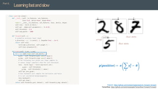
𝒑 𝒑𝒐𝒔𝒊𝒕𝒊𝒗𝒆 = 𝝈
𝒋
𝒚𝒋
𝟐
− 𝜽
30.
TheForward-ForwardAlgorithm
Part 4,
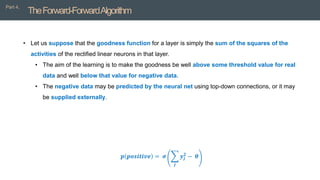
• Letus suppose that the goodness function for a layer is simply the sum of the squares of the
activities of the rectified linear neurons in that layer.
• The aim of the learning is to make the goodness be well above some threshold value for real
data and well below that value for negative data.
• The negative data may be predicted by the neural net using top-down connections, or it may
be supplied externally.
𝒑 𝒑𝒐𝒔𝒊𝒕𝒊𝒗𝒆 = 𝝈
𝒋
𝒚𝒋
𝟐
− 𝜽
31.
TheForward-ForwardAlgorithm
Part 4,
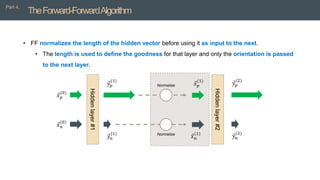
• FFnormalizes the length of the hidden vector before using it as input to the next.
• The length is used to define the goodness for that layer and only the orientation is passed
to the next layer.
Hidden
layer
#1
Ԧ
𝑥𝑝
(0)
Ԧ
𝑥𝑛
(0)
Ԧ
𝑦𝑛
(1)
Ԧ
𝑦𝑝
(1)
Hidden
layer
#2
Normalize
Normalize
Ԧ
𝑥𝑛
(1)
Ԧ
𝑥𝑝
(1)
Ԧ
𝑦𝑛
(2)
Ԧ
𝑦𝑝
(2)
SomeexperimentswithFF
Part 5,
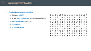
• Thebackpropagation baseline
• Dataset: NMIST
• A few fully connected hidden layers (ReLU)
• No regularizers (dropout)
• 20 epochs
• 1.4% test error
36.
SomeexperimentswithFF
Part 5,
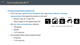
• Asimple unsupervised example of FF
• First, if we have a good source of negative data, does it learn effective multi-layer
representations that capture the structure in the data?
• Random mask 및 1–mask 생성
• hybrid images for the negative data 생성
• NN: four fully connected layers (ReLUs)
• 100 epochs
• softmax
• 1.37% test error
• local receptive fields (without weight-sharing)
• 60 epochs
• 1.16% test error
37.
SomeexperimentswithFF
Part 5,
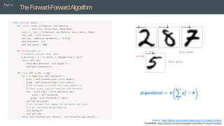
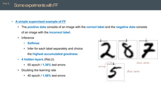
• Asimple supervised example of FF
• The positive data consists of an image with the correct label and the negative data consists
of an image with the incorrect label.
• Inference
• Softmax
• Infer for each label separately and choice
the highest accumulated goodness
• 4 hidden layers (ReLU)
• 60 epoch / 1.36% test errors
• Doubling the learning rate
• 40 epoch / 1.46% test errors
38.
SomeexperimentswithFF
Part 5,
• Asimple supervised example of FF
• train batch = 60000
• test error: 0.06850004196166992
• train batch = 1000
• test error: 0.0755000114440918
• train batch = 100
• test error: 0.9020000025629997
• Batch size 크기가 줄어들수록 오류가 늘어나는 현상이 발생 함
(이미지 처리팀 최승준님 테스트)
39.
SomeexperimentswithFF
Part 5,
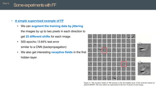
• Asimple supervised example of FF
• We can augment the training data by jittering
the images by up to two pixels in each direction to
get 25 different shifts for each image.
• 500 epochs / 0.64% test error
similar to a CNN (backpropagation)
• We also get interesting receptive fields in the first
hidden layer.
40.
SomeexperimentswithFF
Part 5,
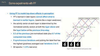
• UsingFF to model top-down effects in perception
• FF’s learned in later layers cannot affect what is
learned in earlier layers. (seems like a major weakness)
• the activity vector at each layer is determined by the
normalized activity vectors at both the layer above and
the layer below at the previous time-step.
• 0.3 of the previous pre-normalized state plus 0.7 of the
computed new state.
• 8 synchronous iterations and picking the label that has
the highest goodness averaged over iterations 3 to 5.
• 60 epochs / 1.31% test error.
41.
ExperimentswithCIFAR-10
Part 5,
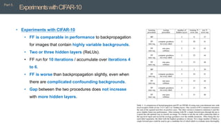
• Experimentswith CIFAR-10
• FF is comparable in performance to backpropagation
for images that contain highly variable backgrounds.
• Two or three hidden layers (ReLUs).
• FF run for 10 iterations / accumulate over iterations 4
to 6.
• FF is worse than backpropagation slightly, even when
there are complicated confounding backgrounds.
• Gap between the two procedures does not increase
with more hidden layers.
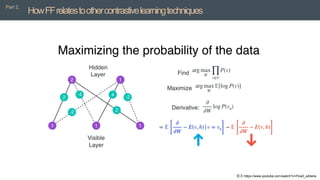
Learningfastandslow
Part 6,
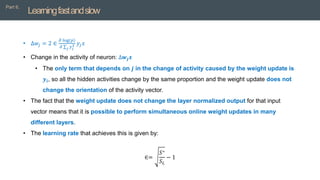
• ∆𝑤𝑗= 2 ∈
𝜕 log 𝑝
𝜕 σ𝑗 𝑦𝑗
2 𝑦𝑗𝑥
• Change in the activity of neuron: ∆𝒘𝒋𝒙
• The only term that depends on 𝒋 in the change of activity caused by the weight update is
𝒚𝒊, so all the hidden activities change by the same proportion and the weight update does not
change the orientation of the activity vector.
• The fact that the weight update does not change the layer normalized output for that input
vector means that it is possible to perform simultaneous online weight updates in many
different layers.
• The learning rate that achieves this is given by:
∈=
𝑆∗
𝑆𝐿
− 1
MortalComputation
Part 7,
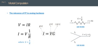
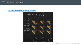
• Therelevance of FF to analog hardware
• An energy efficient way to multiply an activity vector by a weight matrix is to implement
activities as voltages and weights as conductances.
• Unfortunately, it is difficult to implement the backpropagation procedure in an equally efficient
way, so people have resorted to using A-to-D converters and digital computations for
computing gradients.
• FF should make these A-to-D converters unnecessary.
47.
MortalComputation
Part 7,
• Therelevance of FF to analog hardware
𝑉 = 𝐼𝑅
𝐼 = 𝑉
1
𝑅
𝑤ℎ𝑒𝑟𝑒 𝐺 =
1
𝑅
𝐼 = 𝑉𝐺
출력
입력 가중치
𝑉
𝐺 =
1
𝑅
𝐼 = 𝑉𝐺
곱셈 계산방법
𝐼 = 𝐼1 + 𝐼2
𝐼2
𝐼1
덧셈 계산방법
MortalComputation
Part 7,
• Immortal:The knowledge does not die when the hardware dies.
• The software should be separable from the hardware so that the same program or the same
set of weights can be run on a different physical copy of the hardware.
• Mortal: It should be possible to achieve huge savings in the energy required to perform a
computation and in the cost of fabricating the hardware that executes the computation.
• These parameter values are only useful for that specific hardware instance, so the
computation they perform is mortal: it dies with the hardware.
• The function itself can be transferred (approximately) to a different piece of hardware by using
distillation.
참고: https://www.youtube.com/watch?v=sghvwkXV3VU
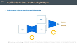
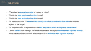
Futurework
Part 8,
• FFproduce a generative model of images or video?
• What is the best goodness function to use?
• What is the best activation function to use?
• For spatial data, can FF benefit from having lots of local goodness functions for different
regions of the image?
• For sequential data, is it possible to use fast weights to mimic a simplified transformer?
• Can FF benefit from having a set of feature detectors that try to maximize their squared activity
and a set of constraint violation detectors that try to minimize their squared activity?


![[PR12] understanding deep learning requires rethinking generalization](https://cdn.slidesharecdn.com/ss_thumbnails/pr12understandingdeeplearningrequiresrethinkinggeneralization-180121135850-thumbnail.jpg?width=640&height=640&fit=bounds)


![[DL輪読会]相互情報量最大化による表現学習](https://cdn.slidesharecdn.com/ss_thumbnails/20190913iwasawa-190913002312-thumbnail.jpg?width=640&height=640&fit=bounds)


![[DL輪読会]A Bayesian Perspective on Generalization and Stochastic Gradient Descent](https://cdn.slidesharecdn.com/ss_thumbnails/20171106dl2-171108033614-thumbnail.jpg?width=640&height=640&fit=bounds)


![[PR12] Inception and Xception - Jaejun Yoo](https://cdn.slidesharecdn.com/ss_thumbnails/pr12inceptionandxception-jaejunyoo-170910140157-thumbnail.jpg?width=640&height=640&fit=bounds)
![[2A4]DeepLearningAtNAVER](https://cdn.slidesharecdn.com/ss_thumbnails/2a4deeplearningatnaver-140929210707-phpapp01-thumbnail.jpg?width=640&height=640&fit=bounds)