The document discusses advanced analytics and data interpretation in digital marketing, emphasizing the complexities behind numerical data and the importance of visualization and experimentation. It provides a step-by-step guide on how to prepare and analyze data using regression and highlights various attribution models while stressing the need for A/B testing. Additionally, it mentions the upcoming Trendigital Summit for further learning on technology and marketing strategies.

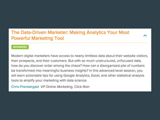
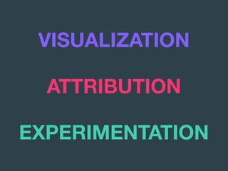
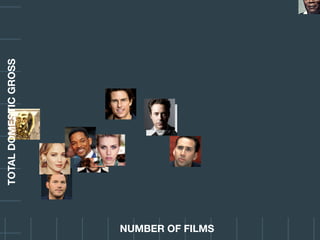
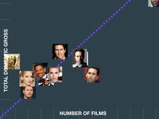
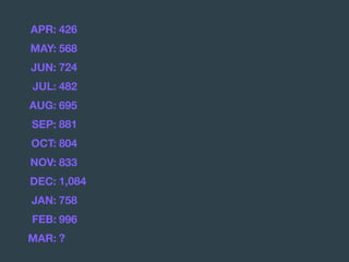
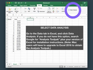
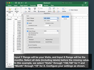
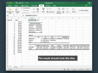
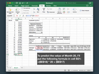
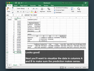
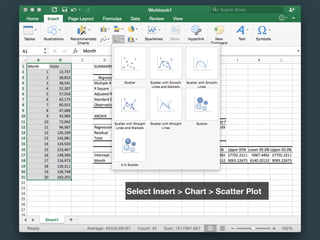
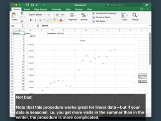
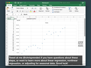
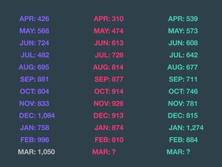
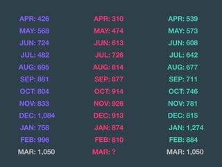
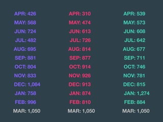
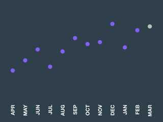
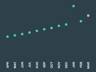
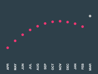
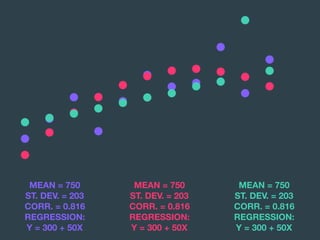
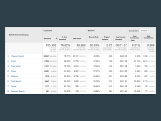
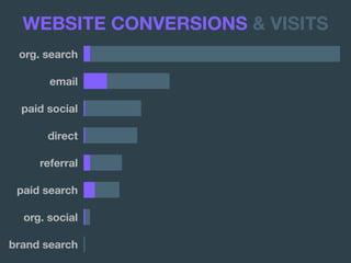
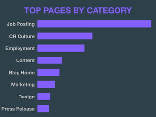
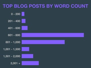
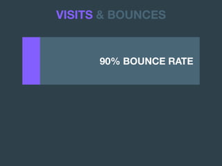
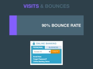
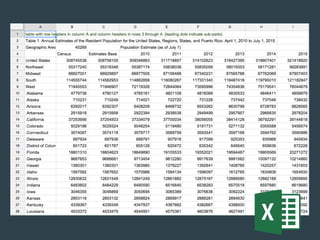
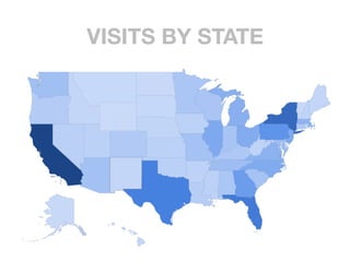
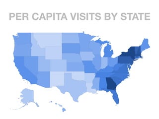
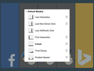
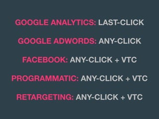
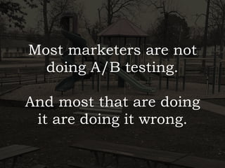
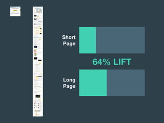
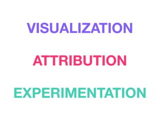
1. @CHRISPRENDER | #TRENDIGITALSF

3. I’M NOT REALLY A
‘NUMBERS PERSON’

4. GROWTH HACKER

5. SOCIAL MEDIA GURU

6. NINJAPRENEUR

8. IT’S ALL NUMBERS

10. WELCOME NERDS

12. ADVANCED ANALYTICS

13. IT’S ACTUALLY MORE
COMPLICATED THAN THAT

15. VISUALIZATION
ATTRIBUTION
EXPERIMENTATION

16. VISUALIZATION

18. A data point tells
you almost nothing.

23. TOTALDOMESTICGROSS

24. TOTALDOMESTICGROSS
NUMBER OF FILMS

25. TOTALDOMESTICGROSS
NUMBER OF FILMS

26. The story behind the
data is more complex
than a single number.

27. APR: 426
MAY: 568
JUN: 724
JUL: 482
AUG: 695
SEP: 881
OCT: 804
NOV: 833
DEC: 1,084
JAN: 758
FEB: 996
MAR: ?

28. APR: 426
MAY: 568
JUN: 724
JUL: 482
AUG: 695
SEP: 881
OCT: 804
NOV: 833
DEC: 1,084
JAN: 758
FEB: 996
MAR: ?
APR: 539
MAY: 573
JUN: 608
JUL: 642
AUG: 677
SEP: 711
OCT: 746
NOV: 781
DEC: 815
JAN: 1,274
FEB: 884
MAR: ?

29. APR: 426
MAY: 568
JUN: 724
JUL: 482
AUG: 695
SEP: 881
OCT: 804
NOV: 833
DEC: 1,084
JAN: 758
FEB: 996
MAR: ?
APR: 539
MAY: 573
JUN: 608
JUL: 642
AUG: 677
SEP: 711
OCT: 746
NOV: 781
DEC: 815
JAN: 1,274
FEB: 884
MAR: ?
APR: 310
MAY: 474
JUN: 613
JUL: 726
AUG: 814
SEP: 877
OCT: 914
NOV: 926
DEC: 913
JAN: 874
FEB: 810
MAR: ?

30. PREPARE YOUR DATA
Find the data you want to predict in Google
Analytics. Copy that data to a new spreadsheet,
and convert the months to numbers. Note: if you
have more than one year of data, the second year
will have to be months 13, 14, 15, etc. rather than
starting back at month 1.

31. SELECT DATA ANALYSIS
Go to the Data tab in Excel, and click Data
Analysis. If you do not have this option, search
Google for “Analysis Toolpak” plus your version of
Excel for installation instructions. (Note: Mac
users will have to upgrade to Excel 2016 to obtain
the Analysis Toolpak.)

32. Select Regression from the menu.

33. Input Y Range will be your Visits, and Input X Range will be the
months. Select all data (including labels) before the missing value.
In this example, we select “Visits” through “158,748” for Y and
“Month” through “19” for X. Configure your settings as shown.

34. The result should look like this.

35. Remember the formula for a line from high
school math? y = mx + b. In this case,
m = slope = cell E18
b = intercept = cell E17.

36. To predict the value of Month 20, I’ll
put the following formula in cell B21:
=($E$18) * 20 + ($E$17)

37. Looks good!
Next you’ll want to visualize the data in columns A
and B to make sure the prediction makes sense.

38. Select Insert > Chart > Scatter Plot

39. Not bad!
Note that this procedure works great for linear data—but if your
data is seasonal, i.e. you get more visits in the summer than in the
winter, the procedure is more complicated.

40. Tweet at me (@chrisprender) if you have questions about these
steps, or want to learn more about linear regression, nonlinear
regression, or adjusting for seasonal data. Good luck!

41. APR: 426
MAY: 568
JUN: 724
JUL: 482
AUG: 695
SEP: 881
OCT: 804
NOV: 833
DEC: 1,084
JAN: 758
FEB: 996
MAR: ?
APR: 539
MAY: 573
JUN: 608
JUL: 642
AUG: 677
SEP: 711
OCT: 746
NOV: 781
DEC: 815
JAN: 1,274
FEB: 884
MAR: ?
APR: 310
MAY: 474
JUN: 613
JUL: 726
AUG: 814
SEP: 877
OCT: 914
NOV: 926
DEC: 913
JAN: 874
FEB: 810
MAR: ?

42. APR: 426
MAY: 568
JUN: 724
JUL: 482
AUG: 695
SEP: 881
OCT: 804
NOV: 833
DEC: 1,084
JAN: 758
FEB: 996
MAR: 1,050
APR: 539
MAY: 573
JUN: 608
JUL: 642
AUG: 677
SEP: 711
OCT: 746
NOV: 781
DEC: 815
JAN: 1,274
FEB: 884
MAR: ?
APR: 310
MAY: 474
JUN: 613
JUL: 726
AUG: 814
SEP: 877
OCT: 914
NOV: 926
DEC: 913
JAN: 874
FEB: 810
MAR: ?

43. APR: 426
MAY: 568
JUN: 724
JUL: 482
AUG: 695
SEP: 881
OCT: 804
NOV: 833
DEC: 1,084
JAN: 758
FEB: 996
MAR: 1,050
APR: 539
MAY: 573
JUN: 608
JUL: 642
AUG: 677
SEP: 711
OCT: 746
NOV: 781
DEC: 815
JAN: 1,274
FEB: 884
MAR: 1,050
APR: 310
MAY: 474
JUN: 613
JUL: 726
AUG: 814
SEP: 877
OCT: 914
NOV: 926
DEC: 913
JAN: 874
FEB: 810
MAR: ?

44. APR: 426
MAY: 568
JUN: 724
JUL: 482
AUG: 695
SEP: 881
OCT: 804
NOV: 833
DEC: 1,084
JAN: 758
FEB: 996
MAR: 1,050
APR: 539
MAY: 573
JUN: 608
JUL: 642
AUG: 677
SEP: 711
OCT: 746
NOV: 781
DEC: 815
JAN: 1,274
FEB: 884
MAR: 1,050
APR: 310
MAY: 474
JUN: 613
JUL: 726
AUG: 814
SEP: 877
OCT: 914
NOV: 926
DEC: 913
JAN: 874
FEB: 810
MAR: 1,050

45. APR
MAY
JUN
JUL
AUG
SEP
OCT
NOV
DEC
JAN
FEB
MAR

46. APR
MAY
JUN
JUL
AUG
SEP
OCT
NOV
DEC
JAN
FEB
MAR

47. APR
MAY
JUN
JUL
AUG
SEP
OCT
NOV
DEC
JAN
FEB
MAR

48. MEAN = 750
ST. DEV. = 203
CORR. = 0.816
REGRESSION:
Y = 300 + 50X
MEAN = 750
ST. DEV. = 203
CORR. = 0.816
REGRESSION:
Y = 300 + 50X
MEAN = 750
ST. DEV. = 203
CORR. = 0.816
REGRESSION:
Y = 300 + 50X

49. Data without
visualization only
tells half the story.

52. IT’S COMPLICATED

53. APR
MAY
JUN
JUL
AUG
SEP
OCT
NOV
DEC
JAN
FEB

54. APR
MAY
JUN
JUL
AUG
SEP
OCT
NOV
DEC
JAN
FEB

56. DOWNLOAD HISTOGRAM
Google Sheets Link
Excel Download
Note: You will need a Google account to use Google
Sheets. To use, click the link above, and go to File >
Make a Copy to create your own personal file.

57. $0
$100
$200
$300
$400
$500
$600
$700
$800
$900
$1000

58. $0
$100
$200
$300
$400
$500
$600
$700
$800
$900
$1000

62. PAID SOCIAL?

63. org. search
email
paid social
direct
referral
paid search
org. social
brand search
WEBSITE CONVERSIONS & VISITS

66. TOP PAGES BY CATEGORY
Job Posting
CR Culture
Employment
Content
Blog Home
Marketing
Design
Press Release

69. TOP BLOG POSTS BY AUTHOR
Paul
Kristina
Michaela
Dawn
Sarah
Sara
Curtis
Carissa

71. TOP BLOG POSTS BY WORD COUNT
0 - 200
201 - 400
401 - 600
601 - 800
801 - 1,000
1,001 - 1,500
1,501 - 2,000
2,001 +

73. Link to Last Year’s Presentation

74. BANK WEBSITES

75. 90% BOUNCE RATE .
VISITS & BOUNCES

76. 90% BOUNCE RATE .
VISITS & BOUNCES

78. current
customer 94% BOUNCE RATE .
VISITS & BOUNCES BY STATUS
not current
customer 50% BOUNCE RATE

79. CONTENT WEBSITES

80. 18%
EMAIL SUBS & VISITS

82. 0FAQ
1FAQ
2FAQ
3FAQ
4FAQ
5FAQ
6FAQ
7FAQ
8FAQ
9FAQ
10FAQ
9%
SUBS & VISITS BY FAQ PAGES
65%

83. 18%
EMAIL SUBS & VISITS

84. VISITS BY STATE

86. DOWNLOAD PER-CAPITA
Google Sheets Link
Excel Download
Note 1: You will need a Google
account to use Google Sheets.
To use, click the link above, and
go to File > Make a Copy to
create your own personal file.
Note 2: Excel does not have a
built-in mapping function, so you
will have to use Google Sheets
to visualize your per-capita data.

87. VISITS BY STATE

88. PER CAPITA VISITS BY STATE

89. VISUALIZATION

90. ATTRIBUTION

91. Attribution is
the number one
digital marketing
trend of 2016.

92. ROI =
REVENUE - COST
COST

93. IT’S NOT ABOUT
THE MONEY

94. IT’S ABOUT
TAKING CREDIT

107. Bing is the
Skinny Pete of your
online marketing
funnel.

108. ROI =
REVENUE - COST
COST

110. By default, Google
Analytics uses last
non-direct click
attribution.

112. There is no one right
attribution model.
But some of them are
definitely wrong.
@avinash

113. LAST-CLICK
ATTRIBUTION

114. FIRST-CLICK
ATTRIBUTION

115. First-click attribution
is like thanking your
first girlfriend at
your wedding.
@avinash

116. FIRST-CLICK
ATTRIBUTION

117. LINEAR
ATTRIBUTION

118. TIME-DECAY
ATTRIBUTION

119. POSITIONAL
ATTRIBUTION

122. G O O G L E ’ S N E X T

124. VIEW-THROUGH
CONVERSIONS

125. GOOGLE ANALYTICS: LAST-CLICK
GOOGLE ADWORDS: ANY-CLICK
FACEBOOK: ANY-CLICK + VTC
PROGRAMMATIC: ANY-CLICK + VTC
RETARGETING: ANY-CLICK + VTC

132. ATTRIBUTION

133. EXPERIMENTATION

135. Most marketers are not
doing A/B testing.
And most that are doing
it are doing it wrong.

136. This
Thursday
Only
Seats
Still
Available
OPEN RATE

137. This
Thursday
Only
Seats
Still
Available
23.5%
26.2%
11% LIFT
OPEN RATE

138. OPEN RATE
This
Thursday
Only
Seats
Still
Available
23.5%
26.2%
11% LIFT

139. Orange Striped Ties
Premium $19 ties, free shipping.
All colors & patterns available.
www.thetiebar.com
CLICK RATE
$19 Orange Striped Ties
Premium ties, free shipping.
All colors & patterns available.
www.thetiebar.com

140. 11.1%
9.6%
CLICK RATE
15% LIFT
Orange Striped Ties
Premium $19 ties, free shipping.
All colors & patterns available.
www.thetiebar.com
$19 Orange Striped Ties
Premium ties, free shipping.
All colors & patterns available.
www.thetiebar.com

141. 11.1%
9.6%
CLICK RATE
Orange Striped Ties
Premium $19 ties, free shipping.
All colors & patterns available.
www.thetiebar.com
$19 Orange Striped Ties
Premium ties, free shipping.
All colors & patterns available.
www.thetiebar.com

144. CONV. RATE

145. CONV. RATE
12.5%
10.4%
20% LIFT

146. CONV. RATE
12.5%
10.4%

147. Make your first A/B
test an A/Z test.

150. You can do minor tests
forever, but only expect
minor results.

152. Short
Page
Long
Page

153. Short
Page
Long
Page
64% LIFT

154. HOW DO YOU KNOW
WHAT WORKED?

155. DOES IT MATTER?

156. You don’t have a
winner when one
variation is winning.

157. Trendigital Summit 2016
Technology and marketing
conference in Sioux Falls.
trendigitalsummit.com
$49 Tech Conference
Trendigital Summit on Jan. 29.
Tickets available now!
trendigitalsummit.com

158. Trendigital Summit 2016
Technology and marketing
conference in Sioux Falls.
trendigitalsummit.com
$49 Tech Conference
Trendigital Summit on Jan. 29.
Tickets available now!
trendigitalsummit.com

159. LIFT = 50%
CONFIDENCE = 37%
Trendigital Summit 2016
Technology and marketing
conference in Sioux Falls.
trendigitalsummit.com
$49 Tech Conference
Trendigital Summit on Jan. 29.
Tickets available now!
trendigitalsummit.com
2 / 20
3 / 20

160. LIFT = 50%
CONFIDENCE = 87%
Trendigital Summit 2016
Technology and marketing
conference in Sioux Falls.
trendigitalsummit.com
$49 Tech Conference
Trendigital Summit on Jan. 29.
Tickets available now!
trendigitalsummit.com
20 / 200
30 / 200

161. LIFT = 50%
CONFIDENCE = 99.9%
Trendigital Summit 2016
Technology and marketing
conference in Sioux Falls.
trendigitalsummit.com
$49 Tech Conference
Trendigital Summit on Jan. 29.
Tickets available now!
trendigitalsummit.com
200 / 2,000
300 / 2,000

162. PEARSON’S
CHI-SQUARED TEST

163. PEARSON’S
CHI-SQUARED TEST
DOWNLOAD CHI-SQUARED
Google Sheets Link
Excel Download
Note: You will need a Google account to use Google
Sheets. To use, click the link above, and go to File >
Make a Copy to create your own personal file.

164. EXPERIMENTATION

165. WE DID IT.

166. VISUALIZATION
ATTRIBUTION
EXPERIMENTATION

167. IT’S COMPLICATED.
BUT NOW WE UNDERSTAND IT
A LITTLE BETTER.
#HAIKU

168. @CHRISPRENDER | #TRENDIGITALSF