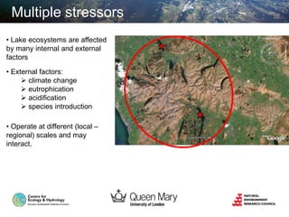
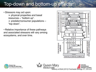
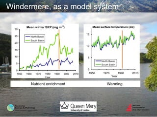
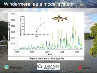
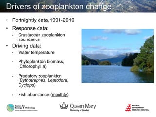
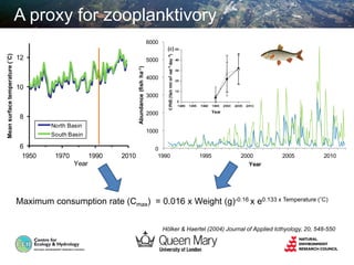
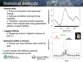
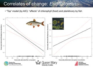
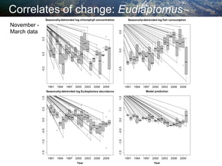
This document summarizes a study analyzing the long-term responses of crustacean zooplankton populations in Windermere, England to multiple stressors including climate change, eutrophication, and the expansion of non-native fish species. The study used statistical models to analyze long-term monitoring data from 1991-2010 on zooplankton abundance, water temperature, phytoplankton biomass, predatory zooplankton, and fish abundance. For the species Eudiaptomus, the top model identified effects of increased chlorophyll (food) and planktivory by fish. While some population change was explained, much variation remained unexplained, warranting further exploration of

1. Disentangling long-term responses of
crustacean zooplankton to multiple
stressors
Stephen J. Thackeray (sjtr@ceh.ac.uk),
Peter Smyntek, Heidrun Feuchtmayr, Ian J. Winfield, Ian D. Jones &
Stephen C. Maberly
Lake Ecosystems Group, Centre for Ecology & Hydrology

2. Multiple stressors
• Lake ecosystems are affected
by many internal and external
factors
• External factors:
 climate change
 eutrophication
 acidification
 species introduction
• Operate at different (local –
regional) scales and may
interact.

3. Top-down and bottom-up effects
Maberly & Elliott (2012) Freshwater Biology, 57, 233-243
• Stressors may act upon:
 physical properties and basal
resources – “bottom up”.
 predator/consumer populations –
“top down”.
• Relative importance of these pathways
and associated stressors will vary among
ecosystems, and over time.

4. Windermere, as a model system
Mean winter SRP (mg m
-3
)
0
5
10
15
20
25
30
1950 1960 1970 1980 1990 2000 2010
Year
North Basin
South Basin
6
8
10
12
1950 1970 1990 2010
Year
Mean surface temperature (oC)
North Basin
South Basin
Nutrient enrichment Warming

5. Windermere, as a model system
0
1000
2000
3000
4000
5000
6000
1990 1995 2000 2005 2010
Abundance(fishha-1)
Year
Expansion of non-native species

6. Focus on crustacean zooplankton
PredatorsGrazersFood/Temperature
• Effects on grazers of long-term
changes in:
 Temperature
 Food (algae)
 Predators (invertebrate)
 Predators (fish)
• Is it possible to detect these
effects on the long-term
dynamics of grazer populations?

7. Drivers of zooplankton change
• Fortnightly data,1991-2010
• Response data:
• Crustacean zooplankton
abundance
• Driving data:
• Water temperature
• Phytoplankton biomass,
(Chlorophyll a)
• Predatory zooplankton
(Bythotrephes, Leptodora,
Cyclops)
• Fish abundance (monthly)

8. A proxy for zooplanktivory
0
1000
2000
3000
4000
5000
6000
1990 1995 2000 2005 2010
Abundance(fishha-1)
Year
6
8
10
12
1950 1970 1990 2010
Year
Mean surface temperature (oC)
North Basin
South Basin
Meansurfacetemperature(˚C)
Maximum consumption rate (Cmax) = 0.016 x Weight (g)-0.16 x e0.133 x Temperature (˚C)
Hölker & Haertel (2004) Journal of Applied Icthyology, 20, 548-550

9. Statistical methods
• Seasonality:
 Focus on long-term (not seasonal)
change.
 Induces correlation among driving
variables.
 Therefore, removed smooth seasonal
“trend” from original data using generalised
additive models (GAMs).
• Lagged effects:
 Response at time t related to drivers at
time t-1.
• Seasonal shifts in drivers:
 Drivers can vary (interact) with month-of-
year.
• Linear models with different predictor
combinations compared by AIC.
°C
Food
Fish

10. Patterns of change: Eudiaptomus

11. Correlates of change: Eudiaptomus
• “Top” model (by AIC): “effects” of chlorophyll (food) and planktivory by fish

12. Correlates of change: Eudiaptomus
November -
March data
1991 1994 1997 2000 2003 2006 2009
-0.20.00.2
Seasonally-detrended log chlorophyll concentration
Year
1991 1994 1997 2000 2003 2006 2009
-0.50.00.5
Seasonally-detrended log fish consumption
Year
1991 1994 1997 2000 2003 2006 2009
-1.5-1.0-0.50.00.51.0
Seasonally-detrended log Eudiaptomus abundance
Year
1991 1994 1997 2000 2003 2006 2009
-1.5-1.0-0.50.00.51.0
Model prediction
Year

13. Summary and next steps
• Can detect a likely effect of increased
planktivory upon Eudiaptomus, though
much unexplained variation.
• Further exploration of the zooplanktivory
“effect”
 sensitivity to parameter choice
 can we apportion planktivory
among fish species?
 is magnitude sufficient to cause
observed population change?
• What about other species?
• Can we see a cascade to the
phytoplankton?
• Independent process modelling studies.

14. Acknowledgements
• This work was funded by NERC
Grant NE/H000208/1: “Whole lake
responses to species invasion
mediated by climate change”
(http://www.windermere-
science.org.uk/).
• Many thanks to everyone involved
in maintaining the Cumbrian
Lakes long-term monitoring
programme, past and present.
• Thank you for your attention!