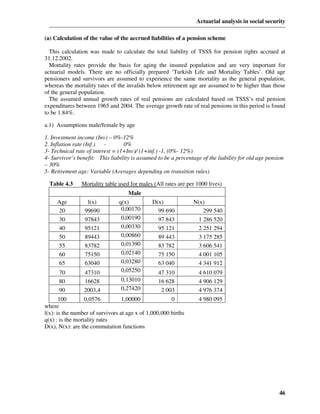
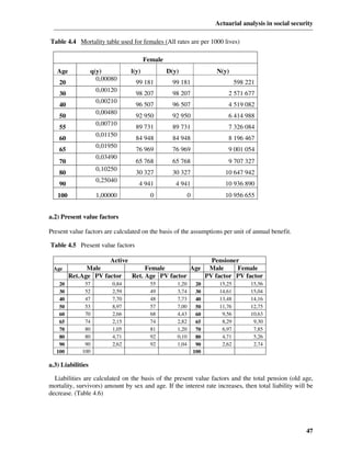
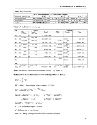
This document is a thesis on actuarial analysis in social security. It acknowledges contributions from various experts who helped with the research. The thesis contains 5 chapters that discuss the role of actuaries in social security, how macroeconomic factors influence calculations, financial aspects of social security systems, an analysis of Turkey's social security system, and some actuarial calculations regarding Azerbaijan's pension system. The conclusion restates that actuaries must analyze complex interacting demographic, economic, financial and legal factors when assessing social security schemes.


![Actuarial analysis in social security
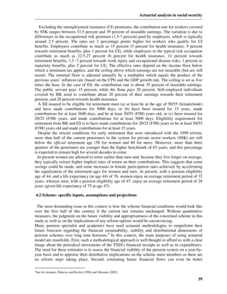
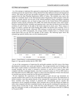
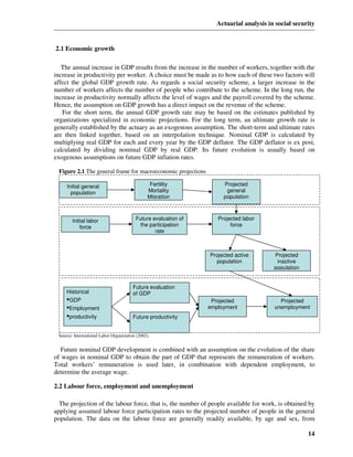
The experience analysis and the economic and demographic prospects indicate areas of
adjustment to the actuarial assumptions. For example, a recent change in retirement behaviour may
induce a new future expected retirement pattern. A slowdown in the economy will require a
database of the number of workers contributing to the scheme. However, as actuarial projections for
pensions are performed over a long period, a change in recently observed data will not necessarily
require any modifications to be made to long-term assumptions. The actuary looks primarily a
consistency between assumptions, and should not give undue weight to recent short-term
conjectural effects.
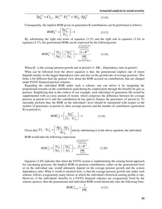
There are 2 actuarial techniques for the analysis of a pension scheme: the projection technique
and the present value technique
1.2.1 – The projection technique
There are different methodologies for social security pension scheme projections. These include:
(a) actuarial methods,
(b) econometric methods and
(c) mixed methods.
Methods classified under (a) have long been applied in the field of insurance and have also proved
valuable for social security projections.
Methods classified under (b) are in effect extrapolations of past trends, using regression
techniques. Essentially the difference between the two is that actuarial methods depend on
endogenous (internal) factors, whereas econometric methods are based on exogenous factors.
Methods classified under (c) rely partly on endogenous and partly on exogenous factors.
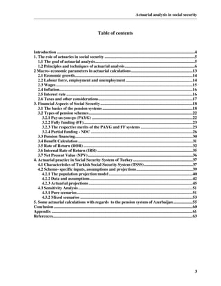
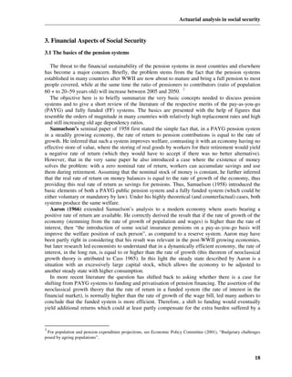
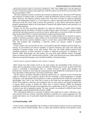
The first step in the projection technique is the demographic projections, production of estimates
of numbers of individuals in each of the principal population subgroups(active insured persons,
retirees, invalids, widows/widowers, orphans )at discrete time-points (t=1,2,..),starting from given
initial values (at t=0).
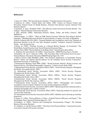
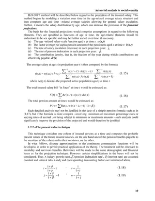
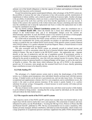
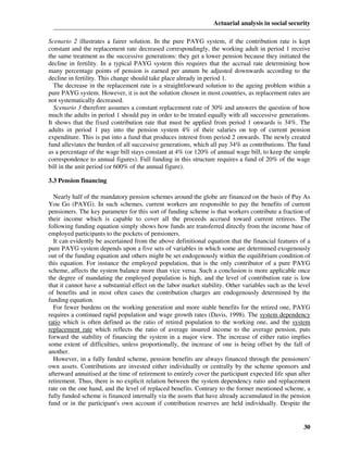
The demographic projection procedure can be regarded as the iteration of a matrix multiplication
operation, typified as follows: 2
nt = nt −1 ⋅ Qt −1 (1.1)
in which nt is a row vector whose elements represent the demographic projection values at time t
and Qt −1 is a square matrix of transition probabilities for the interval (t-1, t) which take the form:
nt = [A(t) R(t) I(t) W(t) O(t)]
(1.2)
p q q q (aa)
q
(ar) (ai) (aw) (ao)
(rr)
0 p 0 q (rw) q (ro)
(1.3)
Qt = 0 0 p (ii) q (iw) q (io)
0 0 0 p (ww) 0
0 0 0 0
p (oo)
The elements of the matrix and the symbols have the following significance:
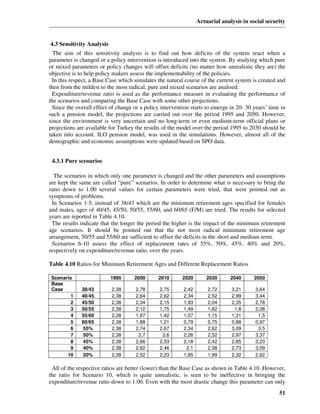
p (rr) denotes the probability of remaining in the same r;
q (rs) denotes the probability of transition from status r to status s;
a, r , i , w and o respectively represent active lives , retirees, invalids, widows/widowers and
orphans .
2
See for instance, Subramaniam Iyer (1999)”Actuarial mathematics of social security pensions” ,International Labour Office
7](https://image.slidesharecdn.com/mbathesis-100820001545-phpapp01/85/MBA-thesis-7-320.jpg)
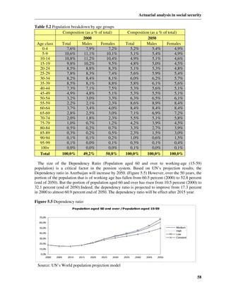
![Actuarial analysis in social security
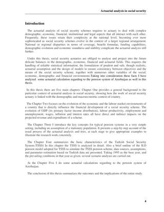
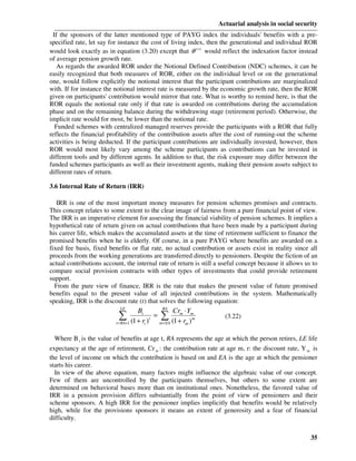
The above procedure, however, is not applied, at the level of total numbers in the subpopulations.
In order to improve precision, each subpopulation is subdivided at least by sex and age. Preferably,
the active population would be further subdivided by past service. The procedure is applied at the
lowest level of subdivision and the results aggregated to give various subtotals and totals. The
matrix Q will be sex-age specific, it can also be varied over time if required. As regards survivors,
an additional procedure is required after each iteration to classify new widows/widowers and
orphans arising from the deaths of males/females aged x according to the age of the
widow/widower or of the orphan before proceeding to the next iteration.
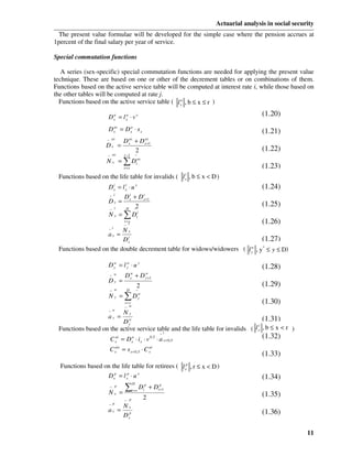
For carrying out the demographic projections it is necessary to adopt an actuarial basis,
consisting of the elements listed below. They should be understood to be sex specific. For brevity,
time is not indicated as a variable, but some or the entire basis may be varied over time.
a - The active table l xa , b ≤ x ≤ r , where b is the youngest entry age and the r the highest
retirement age. This is a double decrement table allowing for the decrements of death and invalidity
only. The associated dependent rates of decrement are denoted by q x (mortality) and i x (invalidity).
a
Retirement is assumed to take place at exact integral ages, just before each birthday, r x denoting the
proportion retiring at age x.
i
b - The life table for invalids l x , b ≤ x < D and the associated independent mortality rate q xi.
c - The life table for retired persons, l xp , r ≤ x < D (where r is the lowest retirement age and D is
p
the death age) and the associated independent rate of mortality q x
d - The double decrement table for widows/widowers, l y , y* ≤ y ≤ D (where y *is the lowest age
w
w
of a widow /widower) and the associated dependent rates of decrement q y (mortality) and
(remarriage) h y
o * *
e - The single decrement table for orphans, l z , 0 ≤ z ≤ z where z is the age limit for orphans’
pensions and the associated independent mortality rate q o z
f - w,x the proportion of married persons among those dying at age x.
g - y x , the average age of the spouse of a person dying at age x.
h - n x , the average number of orphans of a person dying at age x.
i - z x , the average age of the above orphans.
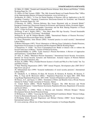
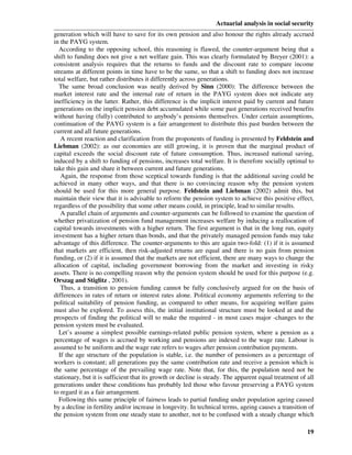
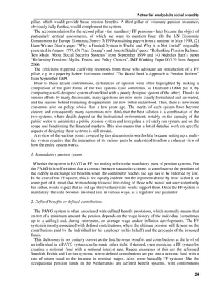
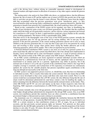
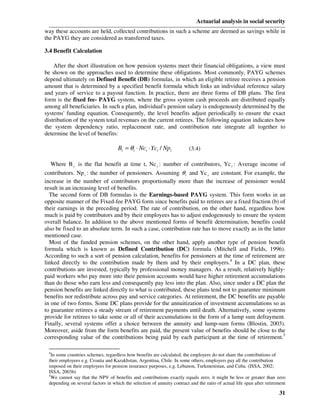
The following expressions for the age and sex – specific one year transition probabilities are
based on the rules of addition and multiplication of probabilities:
Active to active p (aa) = (1 - q a - i x ) ⋅ (1 - rx + 1 )
x x (1.4)
Active to retiree q (ar) = (1 - q a - i x ) ⋅ rx +1
x x
(1.5)
Active to invalid q (ai) = (1 - 0,5 ⋅ q ix ) ⋅ i x
x (1.6)
(1.7)
Active to widow/widower q (aw)x = q (aw1)
x + q (aw2)
x
(1.7.a)
x x [
q (aw1) = q a w x +0,5 1 - 0,5(qwx + hyx )
y ]
1 i
q (aw2) = ix
x
2
[
q x w x +0,75 1 - 0,25(qwx + hyx )
y ] (1.7b
)
Retiree to retiree p (rr) = 1 - q p
x x (1.8)
Retiree to widow/widower x x [
q (rw) = q p w x +0,5 1 - 0,5(qwx + hyx )
y ] (1.9)
8](https://image.slidesharecdn.com/mbathesis-100820001545-phpapp01/85/MBA-thesis-8-320.jpg)
![Actuarial analysis in social security
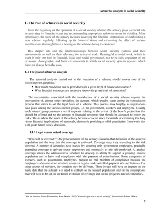
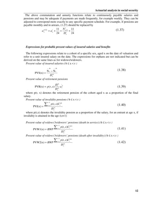
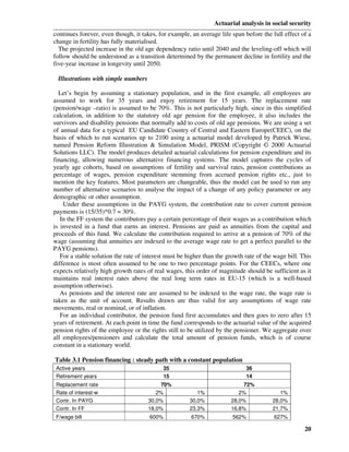
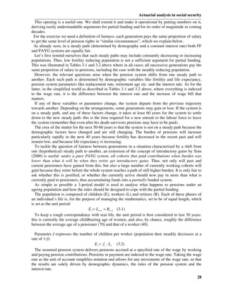
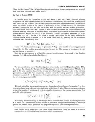
Invalid to invalid p (rr) = 1 - q ix
x (1.10)
Invalid to widow/widower
[
q (iw) = q ix w x +0,5 1 - 0,5(qwx + hyx )
x y ] (1.11)
Widow/widower to widow/widower
p (ww) = 1 - q w - h x
x x (1.12)
Each iteration is assumed to operate immediately after the retirements (occurring at the end of
each year of age).Under the assumption of uniform distribution of decrements over each year of
age, the decrements affecting active persons, retirees and existing invalids –in (1.6),( 1.7a), (1.9)
and (1.11) are assumed to occur, on average at the of six months, new invalids dying before the end
of the year are assumed to die at the end of nine months in (1.7b).
It will be noted that equation (1.7) has two components: (1.7a) relating to deaths of active insured
persons in the age range (x, x+1) and (1.7b) relating to active persons becoming invalid and then
dying at by age x+1. It is understood that the values of w x corresponding to fractional ages which
occur in the above formula would be obtained by interpolation between the values at adjacent
integral ages. Expressions for transition probabilities concerning orphans, corresponding to (1.7a),
(1.7b), (1.9), (1.11) and (1.12) can be derived on the same lines as for widows/widowers.
Starting from the population data on the date of the valuation (t=0), the transition probabilities
are applied to successive projections by sex and age (and preferably by past service , in the new
entrants of the immediately preceding year have to be incorporated before proceeding to the next
iteration. The projection formula for the active insured populations are given below, the method of
projecting the beneficiary populations is illustrated with reference retirement pensioners.
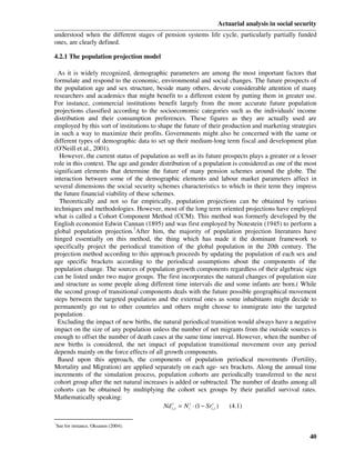
Notation
• Act(x ,s ,t ) denotes the active population aged x nearest birthday , with curtate past service
duration s years at time t, b ≤ x < r, s ≥ 0
• Ac (x , t) denotes the active population aged x nearest birthday at time t. The corresponding
beneficiary populations are denoted by Re(x, t), In (x, t) and Wi (x, t).
• A(t) denotes the total active population at time t. The corresponding beneficiary populations
are denoted by R( t), I (t) and W ( t).
• The number of new entrants aged x next birthday in the projection year t, that is in the
interval (t-1,t ) is denoted by N(x,t)
The projection of the total active and beneficiary populations from time t-1 to time t is
expressed by the equation
r
A(t ) = ∑∑ Act ( x, s, t ) + Act ( x-1,s-1,t-1) ⋅ ( p (aa) − q xar ) − q xai ) − q xaw) − q x )
x-1
( ( ( a
(1.13)
x =b s > 0
D
R (t ) = ∑ Ac(x − 1,t − 1) ⋅ q (ar) + Re(x − 1,t − 1) ⋅ (p (rr) − q x )
x −1 x −1
r
(1.14)
x =r
After the demographic projections is the production of estimates of the total annual insured salary
bill and of the total annual amounts of the different categories of pensions “in force” at discrete
time points (t=1, 2…) starting from given initial values at t=0. These aggregates are obtained by
applying the appropriate per capita average amounts (of salaries or of pensions, as the case may be)
to each individual element of the demographic projections and the summing. The average amounts
are computed year by year in parallel with the progress of the corresponding demographic
projection. An average per capita amount (salary or pension, as the case may be) is computed for
each distinct population element generated by the demographic projection; if different elements are
aggregated in the demographic projection –for example, existing invalids surviving from age x to
x+1 and new invalids reaching age x+1 at the same time –a weighted per capita average amount is
computed to correspond to the aggregated population element.
9](https://image.slidesharecdn.com/mbathesis-100820001545-phpapp01/85/MBA-thesis-9-320.jpg)
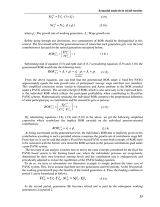
![Actuarial analysis in social security
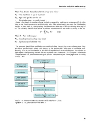
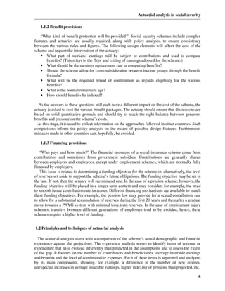
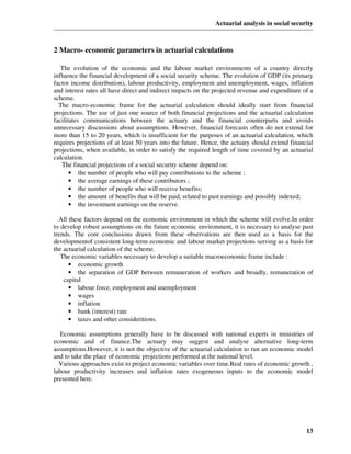
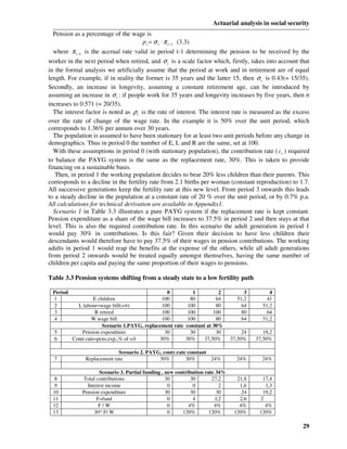
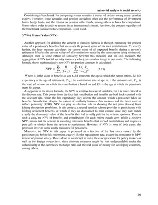
4. Actuarial practice in Social Security System of Turkey
During the last decade, the publicly managed pay-as-you-go (PAYG) pension (old-age insurance)
system in Turkey began to face serious financial difficulties due to generosity of pension benefits
relative to contributions, combined with unrealistically low statutory entitlement ages. When the
deficits generated by the system exceeded tolerable limits, a major pension reform bill was
prepared to set key program parameters straight.
Taking 1995 as the base year, and the prevailing conditions in that year as given, several scenario
analyses are carried out. A pension model that is based on the contribution and pension
characteristics of Turkey, such as the minimum retirement age, minimum contribution period,
replacement ratio, contribution rate, etc., and Turkish demographic and labor market data are used
in system simulation. Scenario analysis indicates that even with scenarios, with no shocks
introduced to the system, it is financially possible for the system to be viable.
4.1 Characteristics of Turkish Social Security System (TSSS)
Old-age insurance operations of the publicly managed social security system in Turkey were set
up in the 1940s to offer universal coverage to workers employed by public and private sectors alike.
The system is made up of three different and distinct branches, each providing pension benefits in
return for compulsory participation in retirement plans run on a pay-as-you-go (PAYG) basis. Prior
to 2003, additional coverage on a voluntary basis was only available through a number of private
pension funds set up by some companies, banks etc. to provide optional coverage to their own
employees. Following the completion of legal and regulatory framework to allow working
individuals to voluntarily purchase optional retirement plans from private companies in 2002, most
insurance companies began to sell optional coverage through money purchase schemes in 2003.
The initial TSSS law allows providing five types of insurance:
I- Insurance against natural disability old age and death.
II- Insurance against work injuries and occupational diseases.
III- Insurance against temporary disability due to sickness or motherhood.
IV- Health insurance for the worker and his/her dependent.
V- Unemployment.
Although the TSSS provides only the first two types of insurance coverage, the attention toward
this corporation has increased substantially from the time it was established especially if the
substitute provisions are absent and the private insurance system in Turkey is still immature and
needs imminent reform.
According to State Planning Organization of Republic of Turkey, 48-50 percent of the workers in
Turkey have social security coverage. There are three major publicly administered social security
institutions, with a combined pool of over 14.3 million active participants in 2006. These are the
Social Insurance Institution [Sosyal Sigortalar Kurumu (SSK)], which is open to private sector
employees and workers in the public sector, Retirement Fund [Emekli Sandigi(ES)], which covers
civil servants, and Bag-Kur (BK), which is a fund for the self-employed. Approximately 59 percent
of the insured population is covered by SSK, 17 percent by ES, and 24 percent by BK. The share of
privately insured individuals is a trivial 0.5 percent in the population.
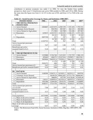
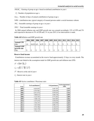
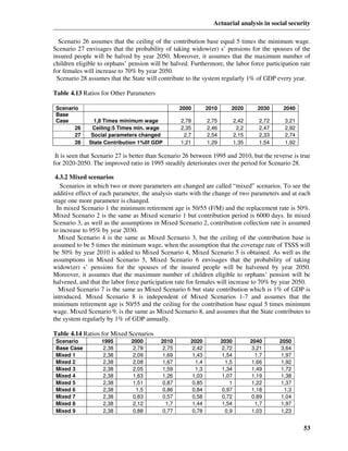
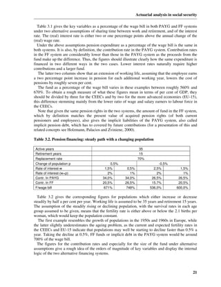
The data in Table 1 provide additional information on the three main components, and trace out
the evolution of the system. In 1980 there were close to 1.3 million pensioners, implying
approximately one pension recipient for 3.65 contributors to the pay-as-you-go system. In 2006 the
number of pensioners exceeded 7.7 million, and the number of contributors per pensioner was
down to 2. The situation is especially acute in the case of SSK and ES, where the ratio of
37](https://image.slidesharecdn.com/mbathesis-100820001545-phpapp01/85/MBA-thesis-37-320.jpg)