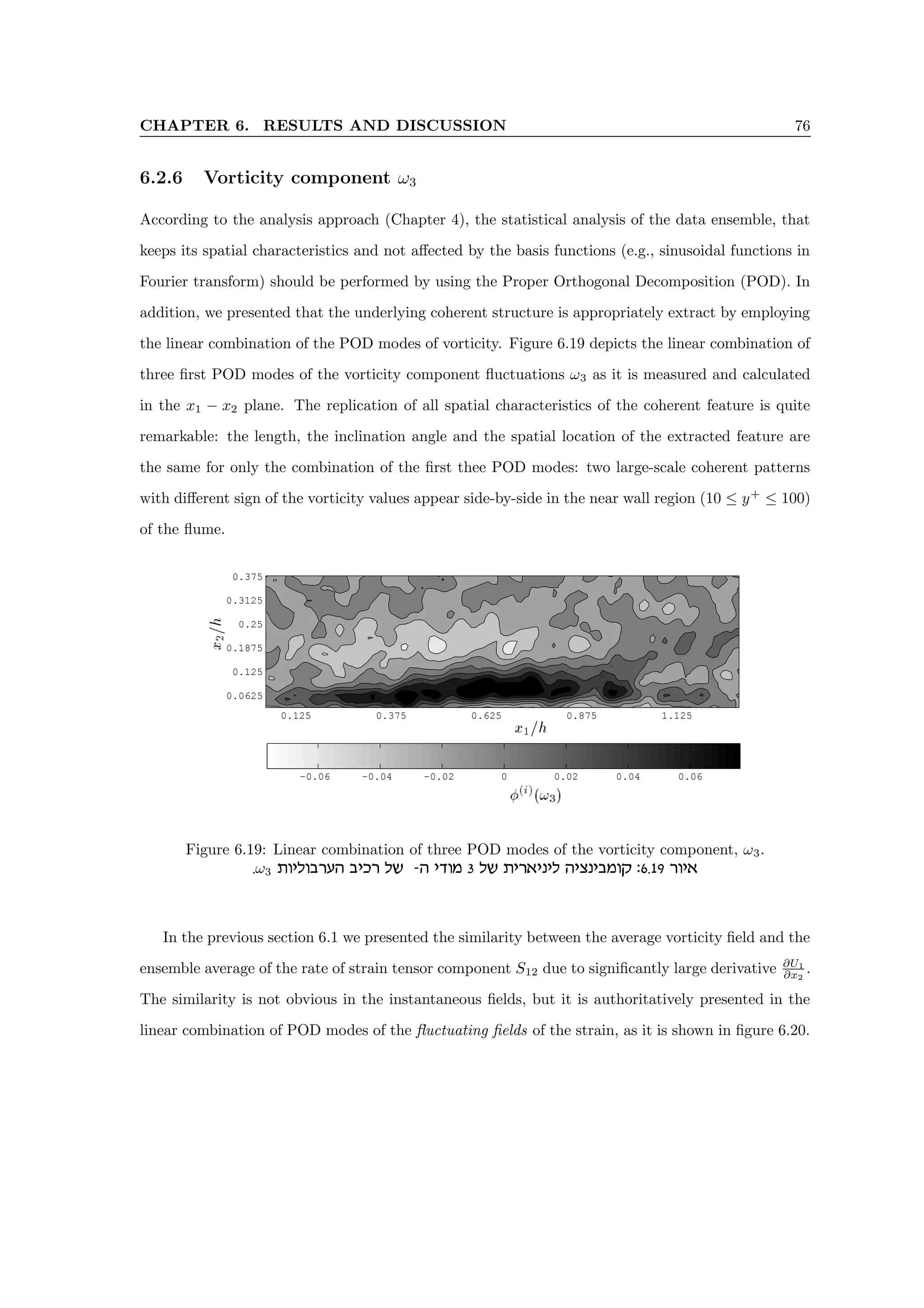
This research thesis by Alex Liberzon focuses on the characterization of coherent structures in turbulent flow, contributing to the understanding of turbulence through comprehensive literature reviews and experimental techniques. It includes detailed mathematical backgrounds and analysis approaches, along with results from various experimental setups like stereoscopic PIV systems. The findings aim to provide insights into coherent structures in turbulent flows and suggest areas for further research.
![LIST OF FIGURES ix
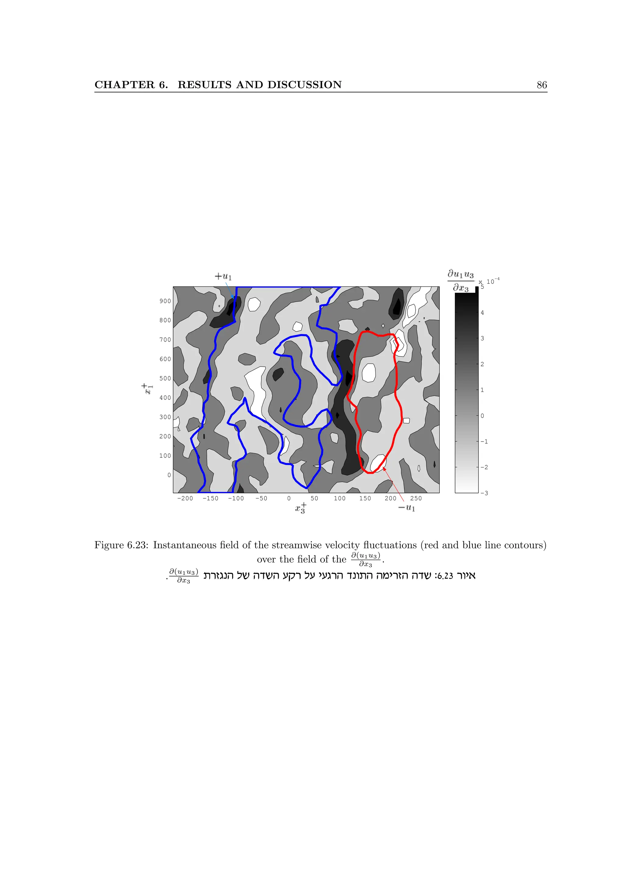
6.23 Instantaneous field of the streamwise velocity fluctuations (red and blue line contours)
over the field of the ∂(u1u3)
∂x3
. . . . . . . . . . . . . . . . . . . . . . . . . . . . . . . . . 86
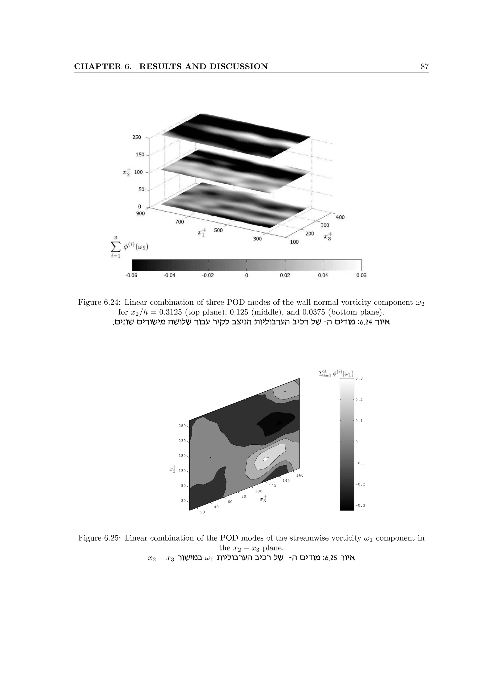
6.24 Linear combination of three POD modes of the wall normal vorticity component ω2
for x2/h = 0.3125 (top plane), 0.125 (middle), and 0.0375 (bottom plane). . . . . . . 87
6.25 Linear combination of the POD modes of the streamwise vorticity ω1 component in
the x2 − x3 plane. . . . . . . . . . . . . . . . . . . . . . . . . . . . . . . . . . . . . . 87
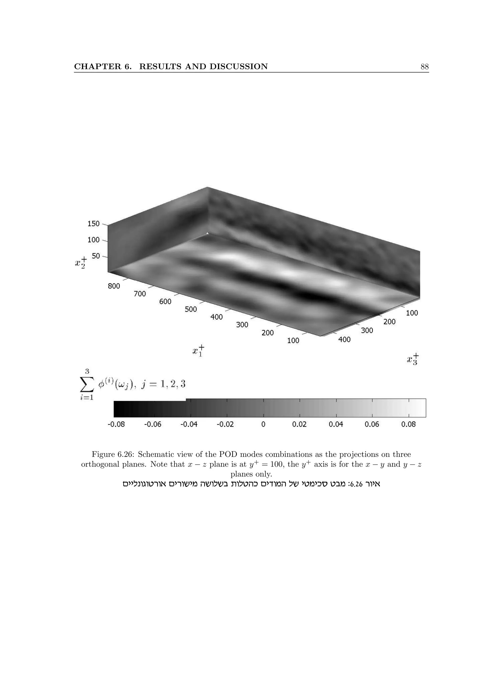
6.26 Schematic view of the POD modes combinations as the projections on three orthog-
onal planes. Note that x − z plane is at y+
= 100, the y+
axis is for the x − y and
y − z planes only. . . . . . . . . . . . . . . . . . . . . . . . . . . . . . . . . . . . . . . 88
6.27 Streamwise velocity average profiles measured by using XPIV (-o) and box-plot of the
PIV measurements in separate y planes(|-[]-|). . . . . . . . . . . . . . . . . . . . . 89
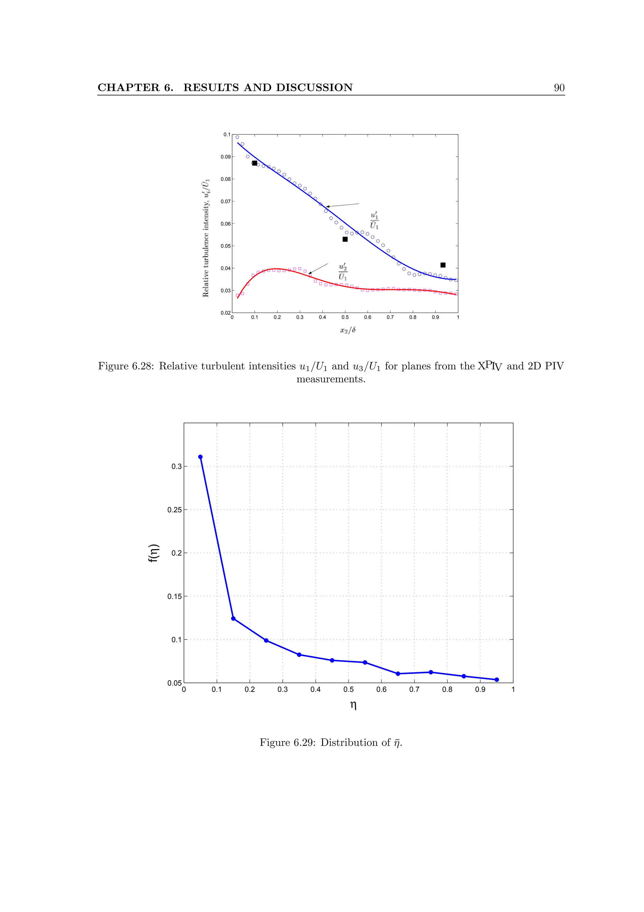
6.28 Relative turbulent intensities u1/U1 and u3/U1 for planes from the XPIV and 2D PIV
measurements. . . . . . . . . . . . . . . . . . . . . . . . . . . . . . . . . . . . . . . . 90
6.29 Distribution of η̄. . . . . . . . . . . . . . . . . . . . . . . . . . . . . . . . . . . . . . 90
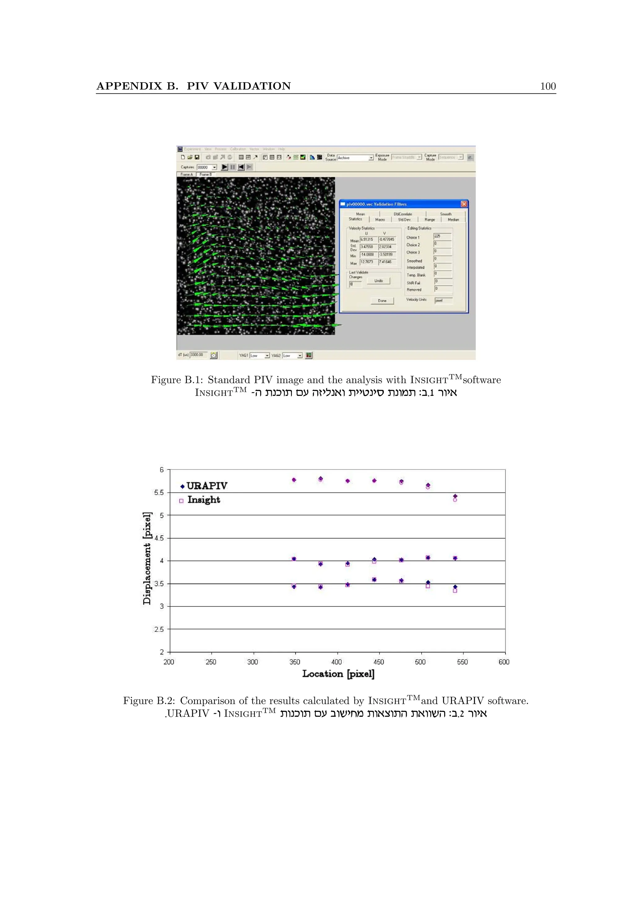
B.1 Standard PIV image and the analysis with InsightTM
software . . . . . . . . . . . . 100
B.2 Comparison of the results calculated by InsightTM
and URAPIV software. . . . . . 100
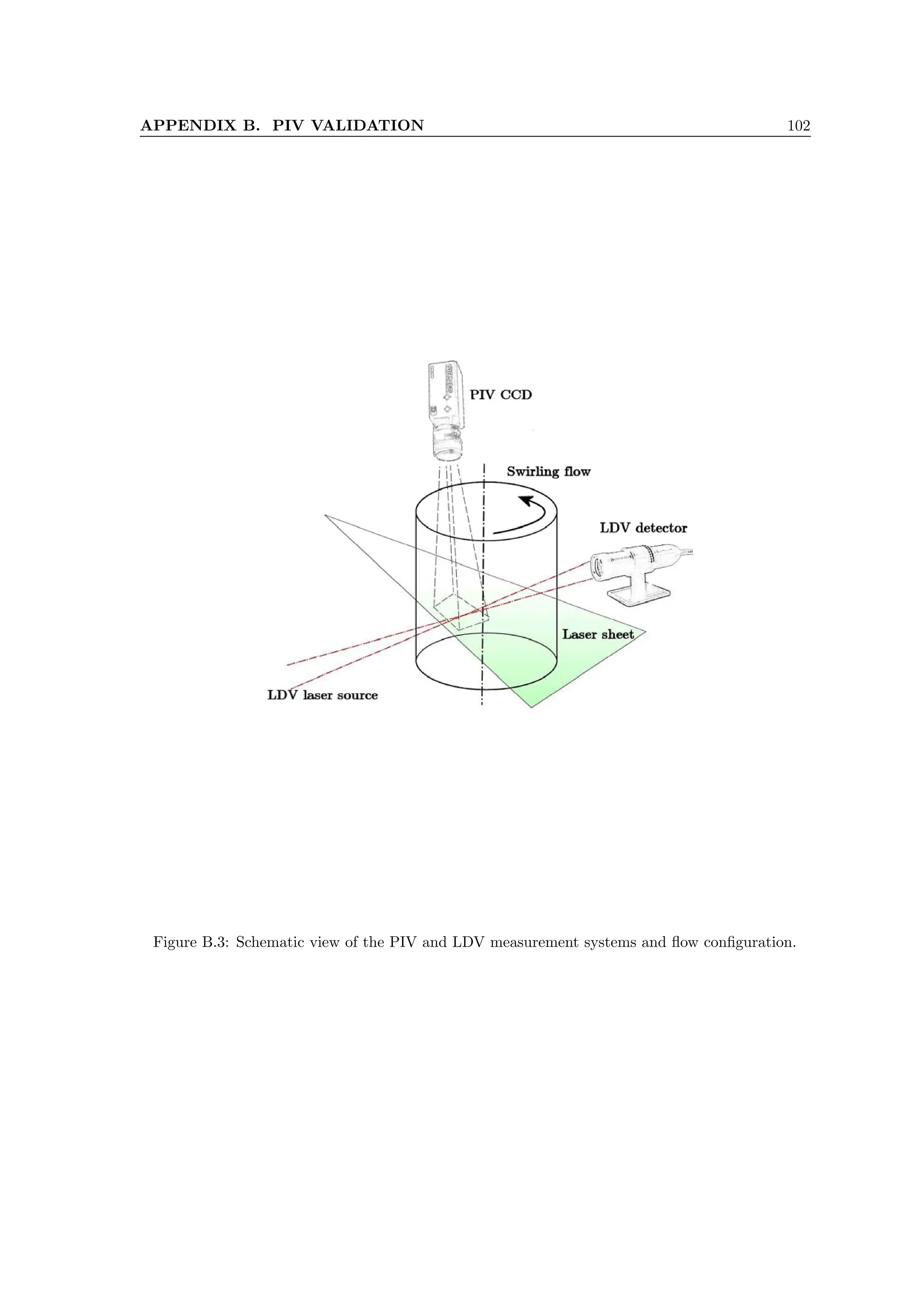
B.3 Schematic view of the PIV and LDV measurement systems and flow configuration. . 102
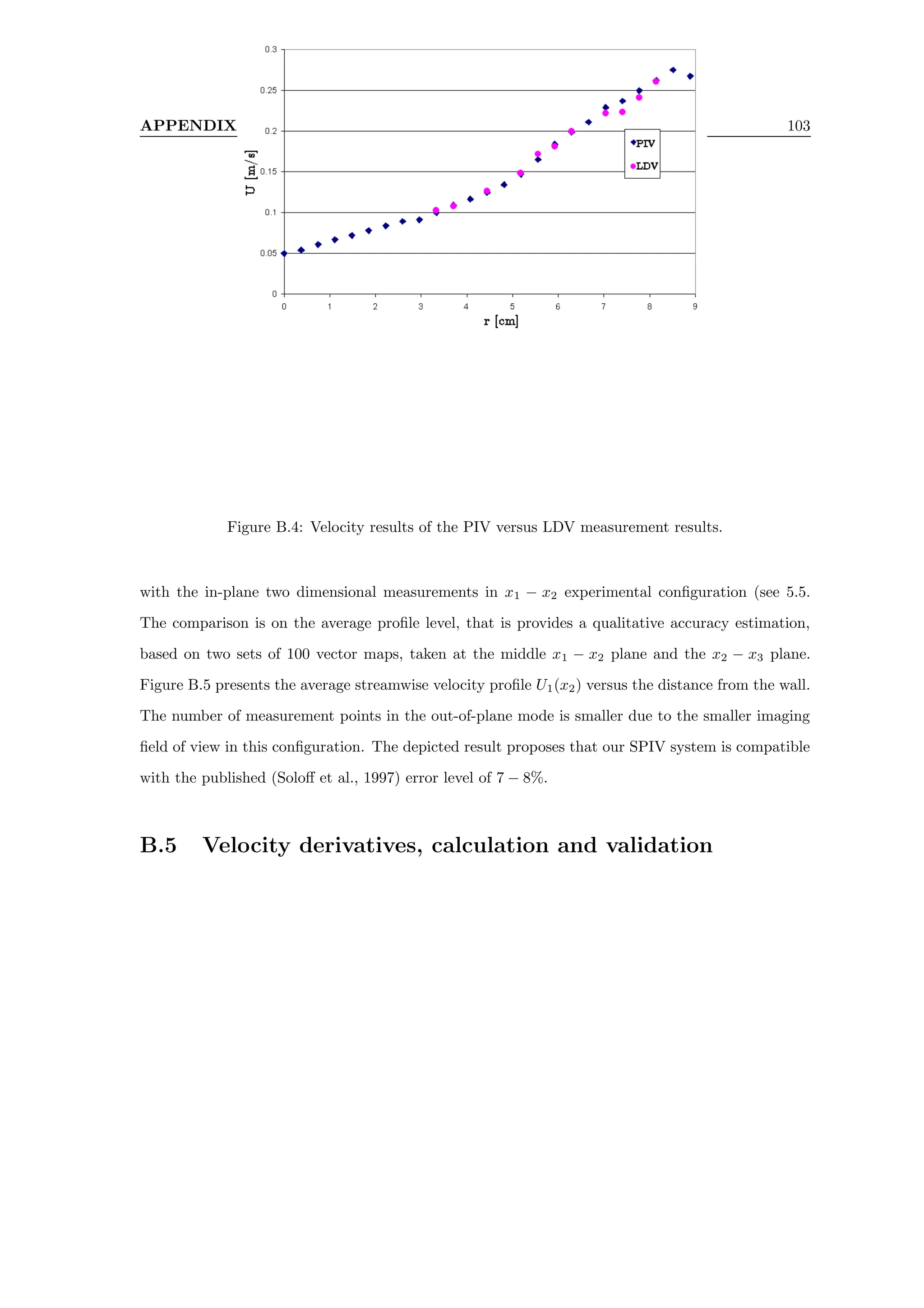
B.4 Velocity results of the PIV versus LDV measurement results. . . . . . . . . . . . . . 103
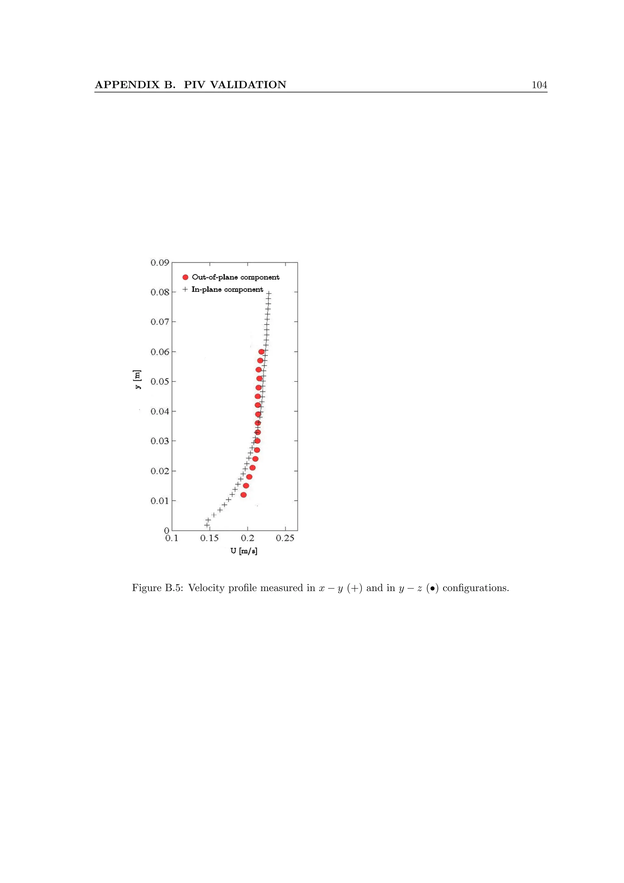
B.5 Velocity profile measured in x − y (+) and in y − z (•) configurations. . . . . . . . . 104
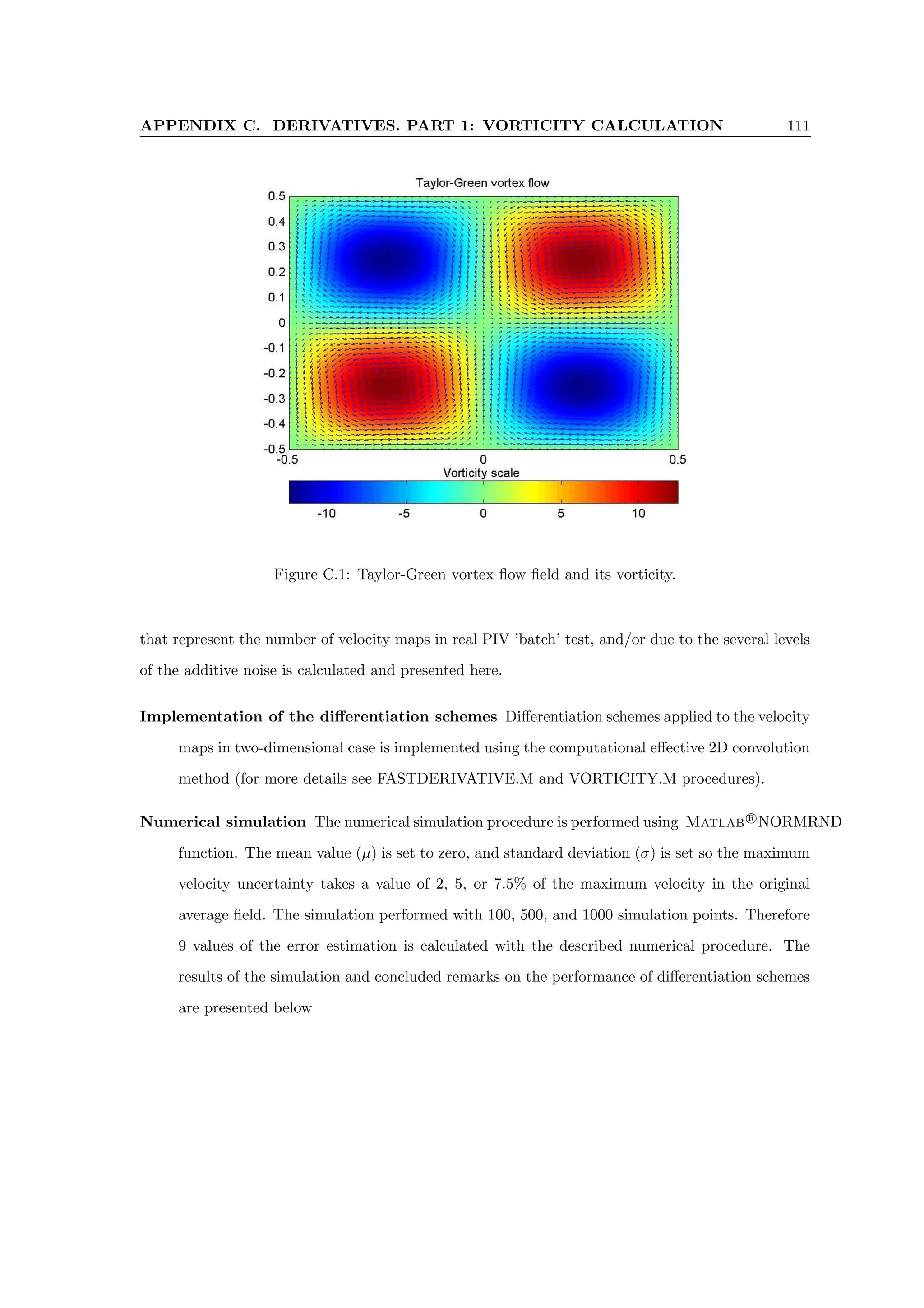
C.1 Taylor-Green vortex flow field and its vorticity. . . . . . . . . . . . . . . . . . . . . . 111
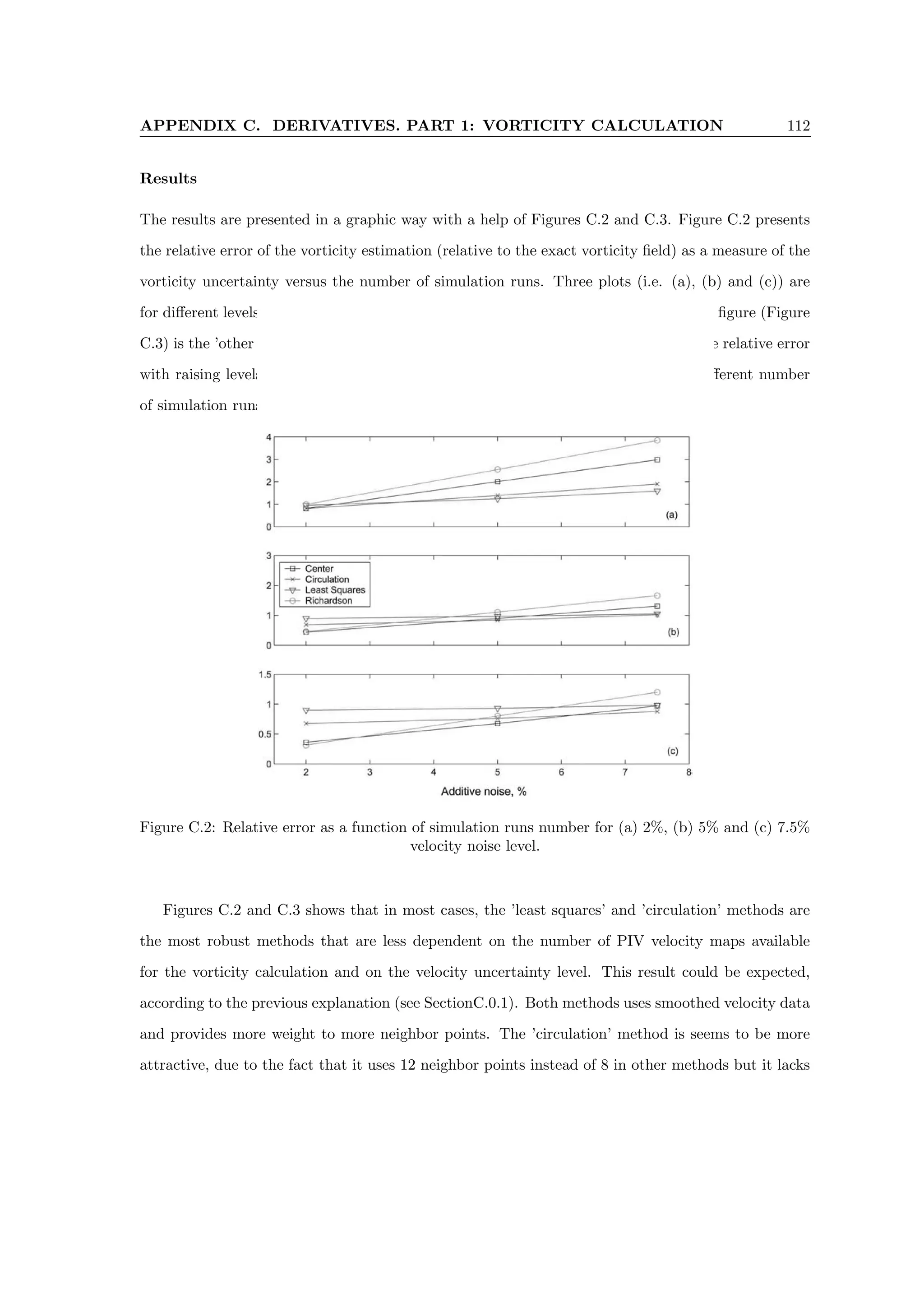
C.2 Relative error as a function of simulation runs number for (a) 2%, (b) 5% and (c)
7.5% velocity noise level. . . . . . . . . . . . . . . . . . . . . . . . . . . . . . . . . . . 112
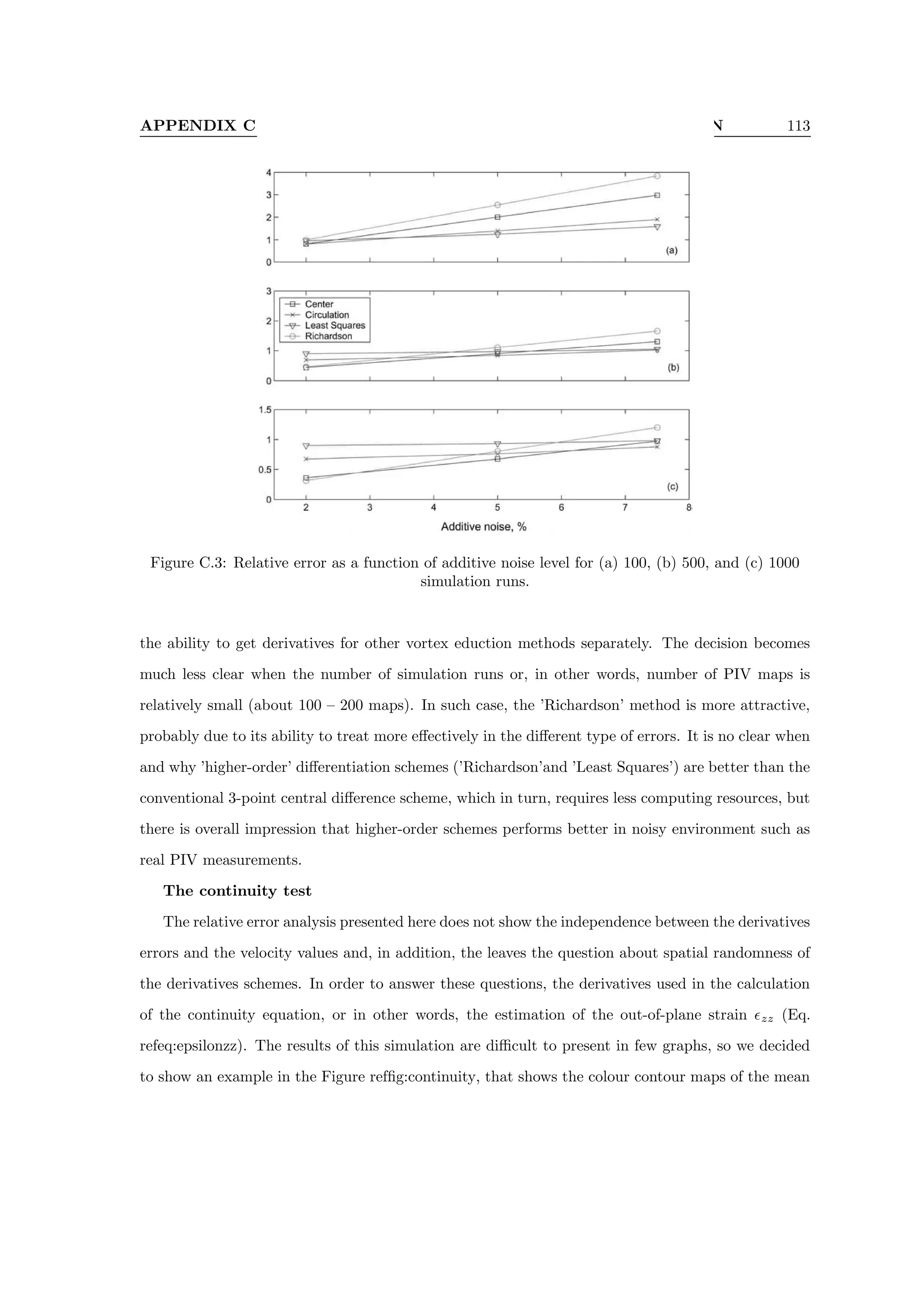
C.3 Relative error as a function of additive noise level for (a) 100, (b) 500, and (c) 1000
simulation runs. . . . . . . . . . . . . . . . . . . . . . . . . . . . . . . . . . . . . . . . 113
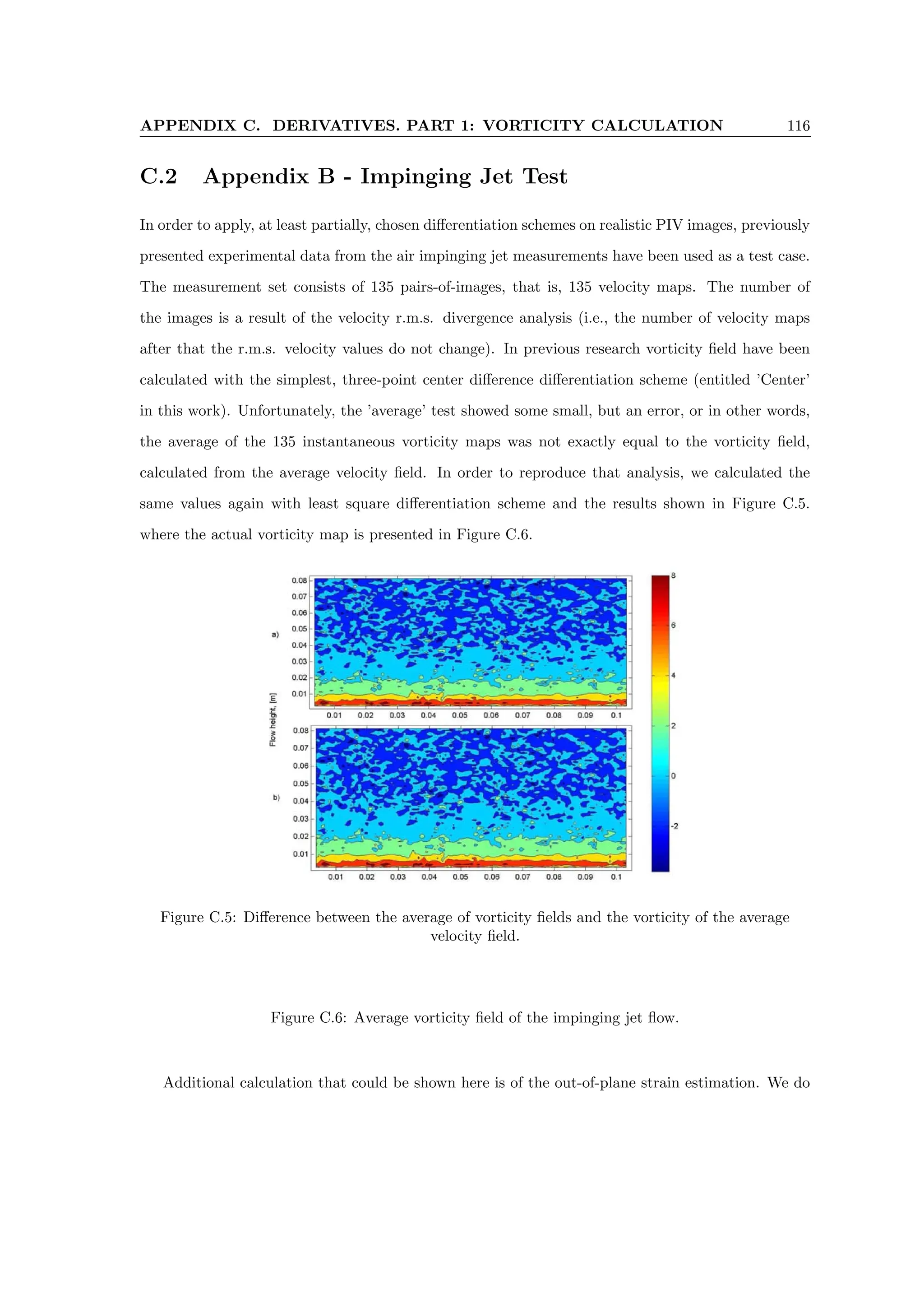
C.4 Mean value of the out-of-plane strain estimation (the mean error of the continuity
equation) for the 500 simulation runs and 5% additive noise level. The plot consists
of the results for the ’Center’ - upper left, ’Richardson’ - upper right, ’Least Squares’
- lower left, and ’Circulation’ calculation scheme at the lower right corner. . . . . . . 114](https://image.slidesharecdn.com/alexliberzonphdthesisweb-240511095654-b7f38227/75/Coherent-structures-characterization-in-turbulent-flow-10-2048.jpg)

![CHAPTER 2. LITERATURE REVIEW 16
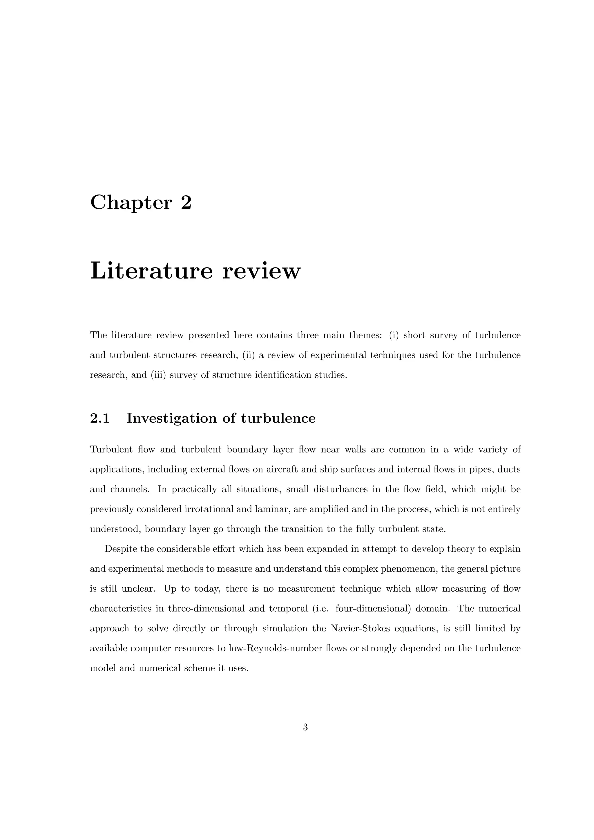
2.4.6 Calculations
Lumley (1970) introduced the Karhunen-Loéve decomposition method of the random functions to
the turbulent flow research to use it as an unbiased method for discrete data set, such as experimental
or numerical data. It is known that in the continuous case the probability density function (PDF)
provides the full description of the of continuous random functions. The integral of the PDF defines
the mean value of the random vector, and the distribution of the random vectors around the mean
is determined by using the covariance matrix. The optimal presentation of the random set defined
above is based on the eigenvectors and eigenvalues of the the covariance matrix.
In the discrete case (such as PIV or DNS data) the flow quantities are presented as the set
of (random) vectors that approves the second order statistical property – the existence of optimal
representation by eigenfunctions. If the set of M vectors of length n is presented as:
{ui}
M
i=1 , ui = [u1, u2, . . . , un]T
(2.13)
then the discrete approximation of the autocorrelation kernel R is known as the covariance matrix:
C =
1
M
M
X
i=1
ui · uT
i (2.14)
Herein we assume the the data is the field of fluctuations, treated as random data. If the data
analysis is of the instantaneous flow quantity (such as instantaneous velocity or vorticity, for in-
stance), then first the statistical average (denoted by¯or by h·i, interchangeably) is calculated by
the approximation:
ū =
1
M
M
X
i=1
ui (2.15)
and then is subtracted from the data vector set:
ui = ui − ū (2.16)
Then the analysis is done by using the fluctuating field, similar to the spatio-temporal data analysis
performed by Heiland (1992). We point out that the covariance matrix is an N × N matrix, where
N is the spatial resolution of a vector (e.g., for the PIV data it is the total number of the vectors
within the flow field). For large N (e.g., N = 1000 vectors for the usual PIV analysis), the covariance
matrix becomes too large for massive computation. In practice, most of the POD analysis, shown](https://image.slidesharecdn.com/alexliberzonphdthesisweb-240511095654-b7f38227/75/Coherent-structures-characterization-in-turbulent-flow-28-2048.jpg)
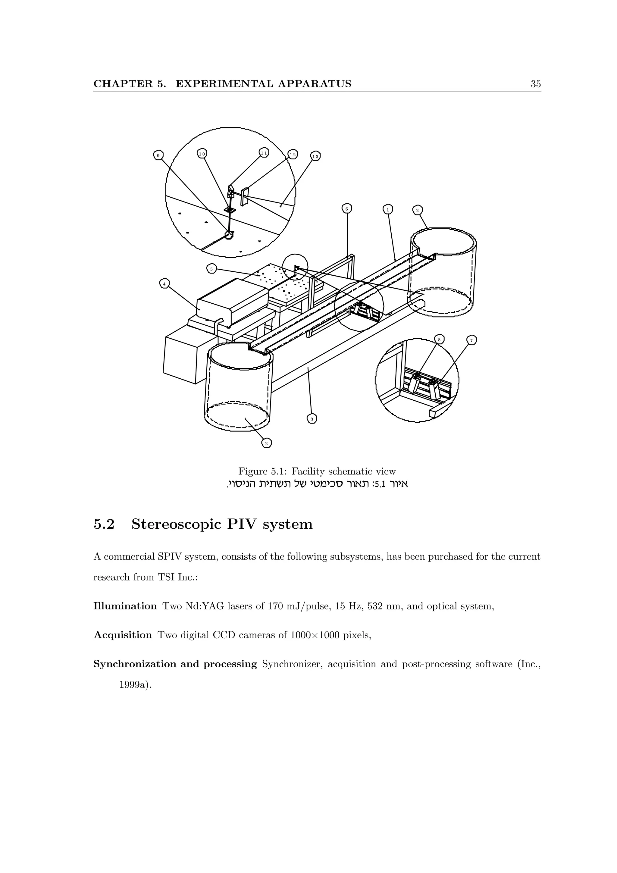
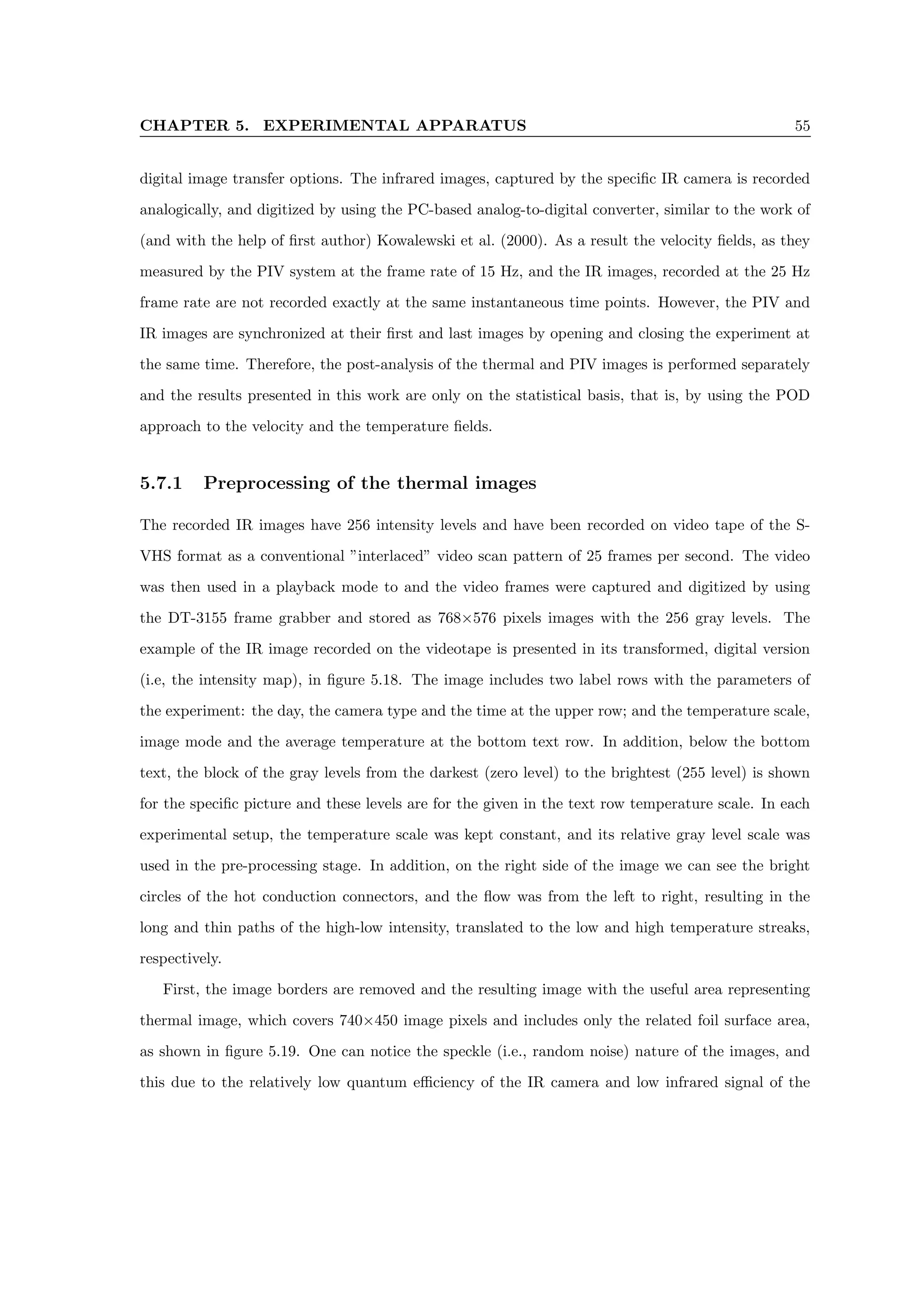
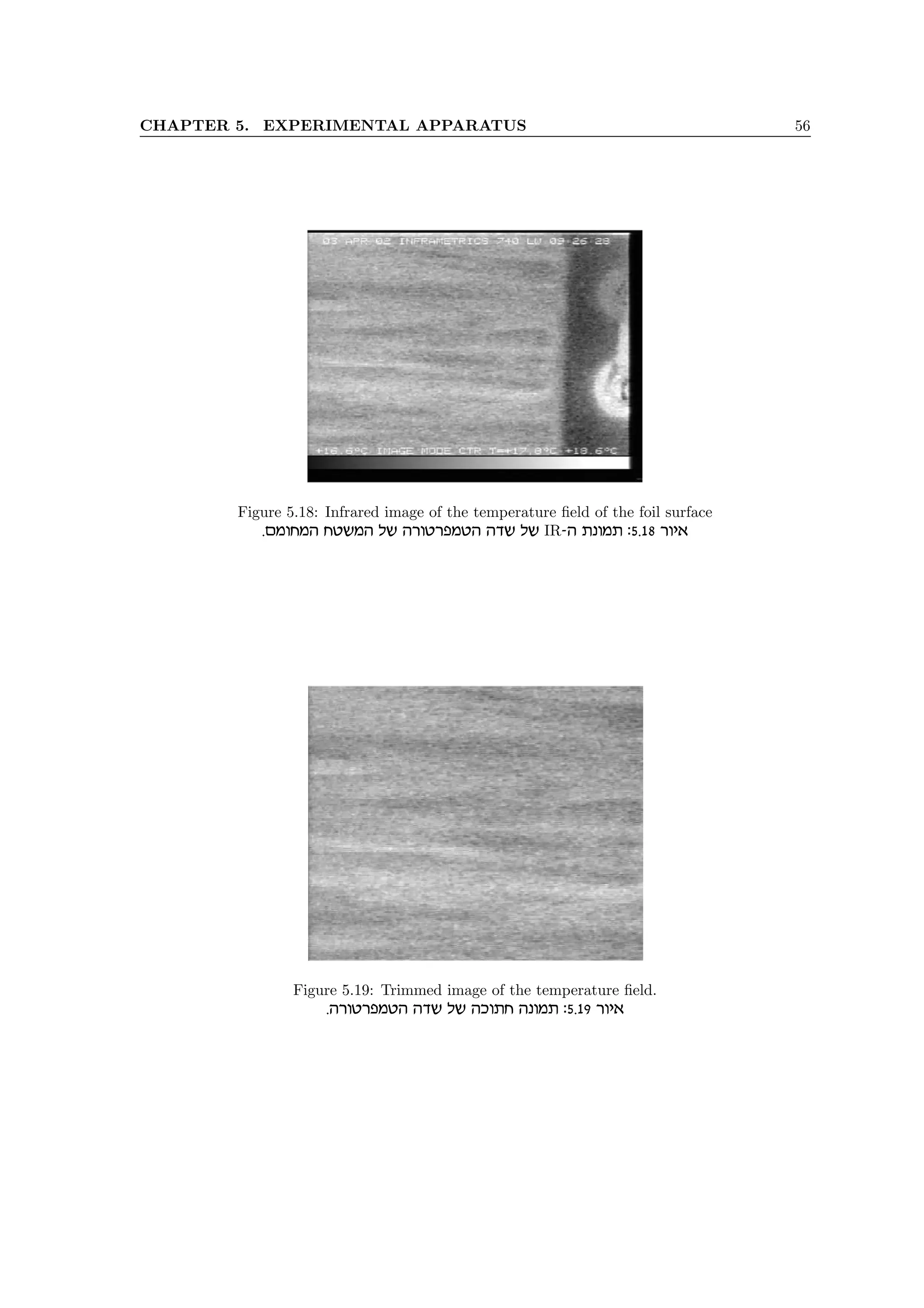
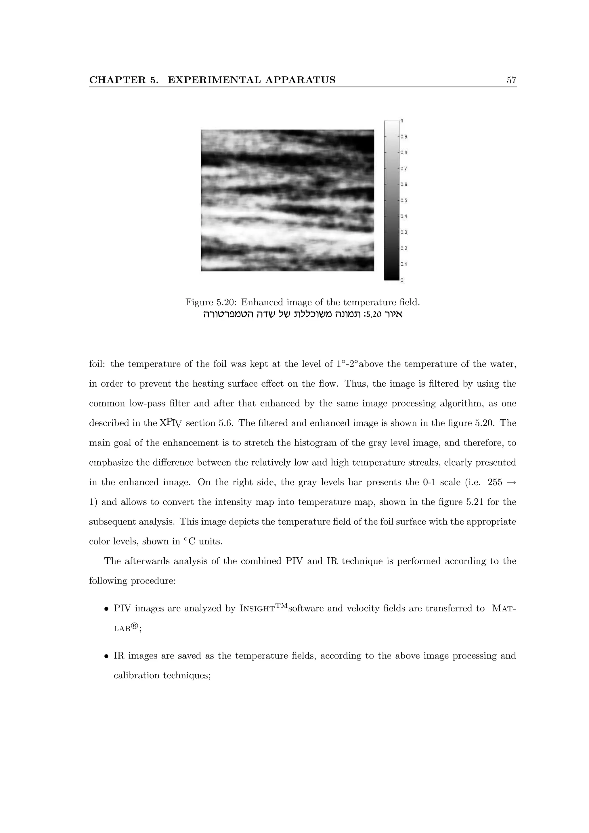
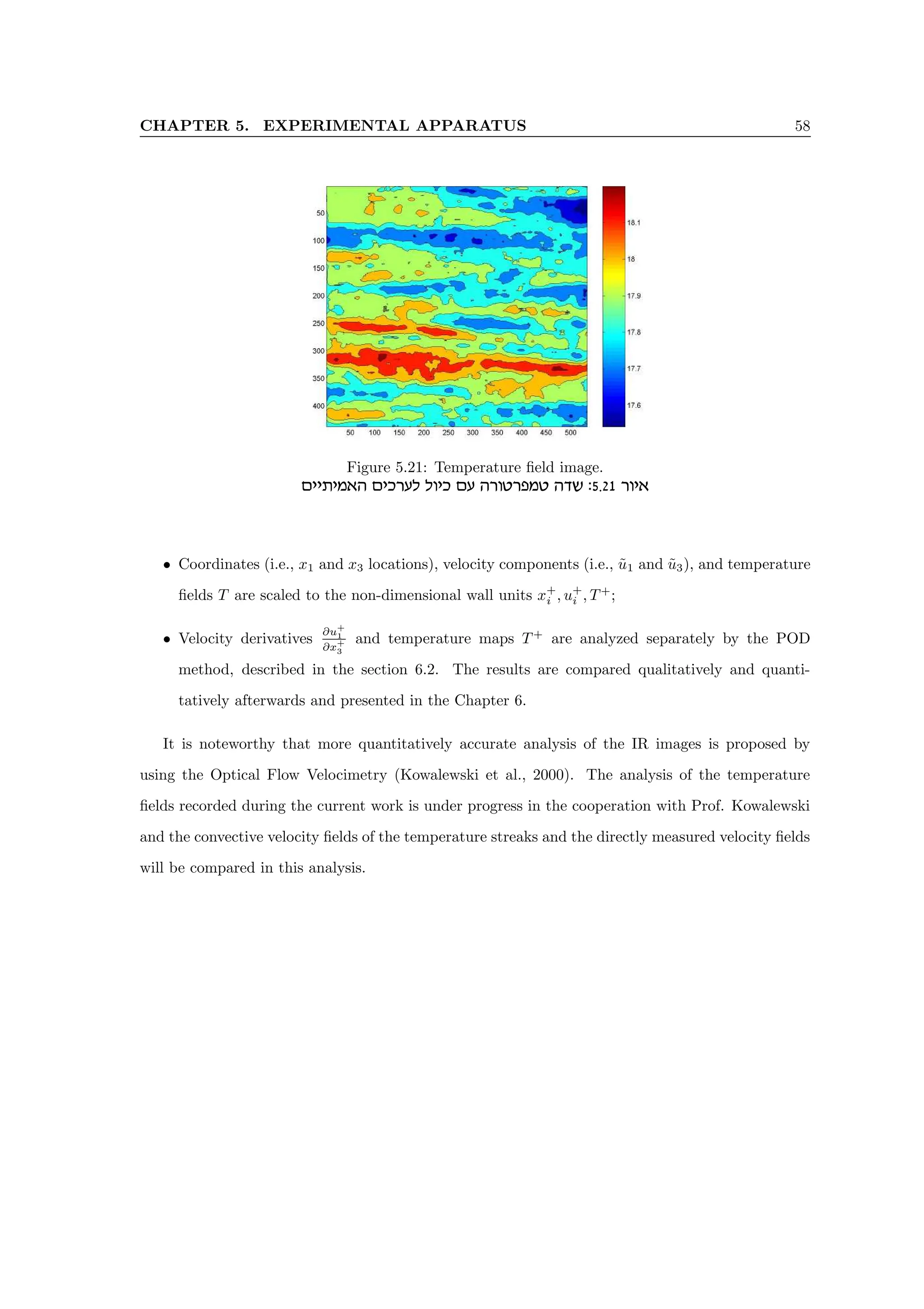
![CHAPTER 5. EXPERIMENTAL APPARATUS 41
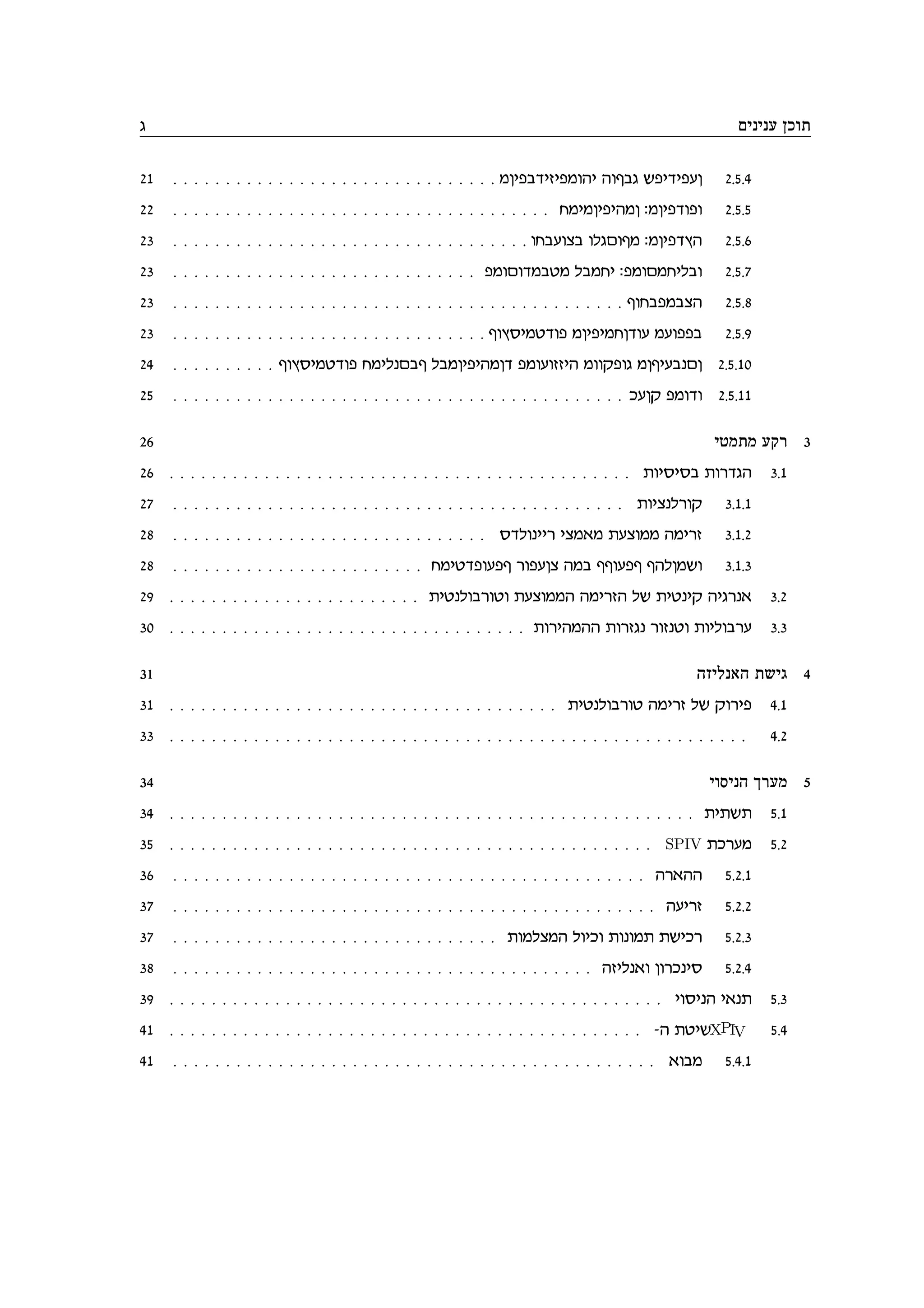
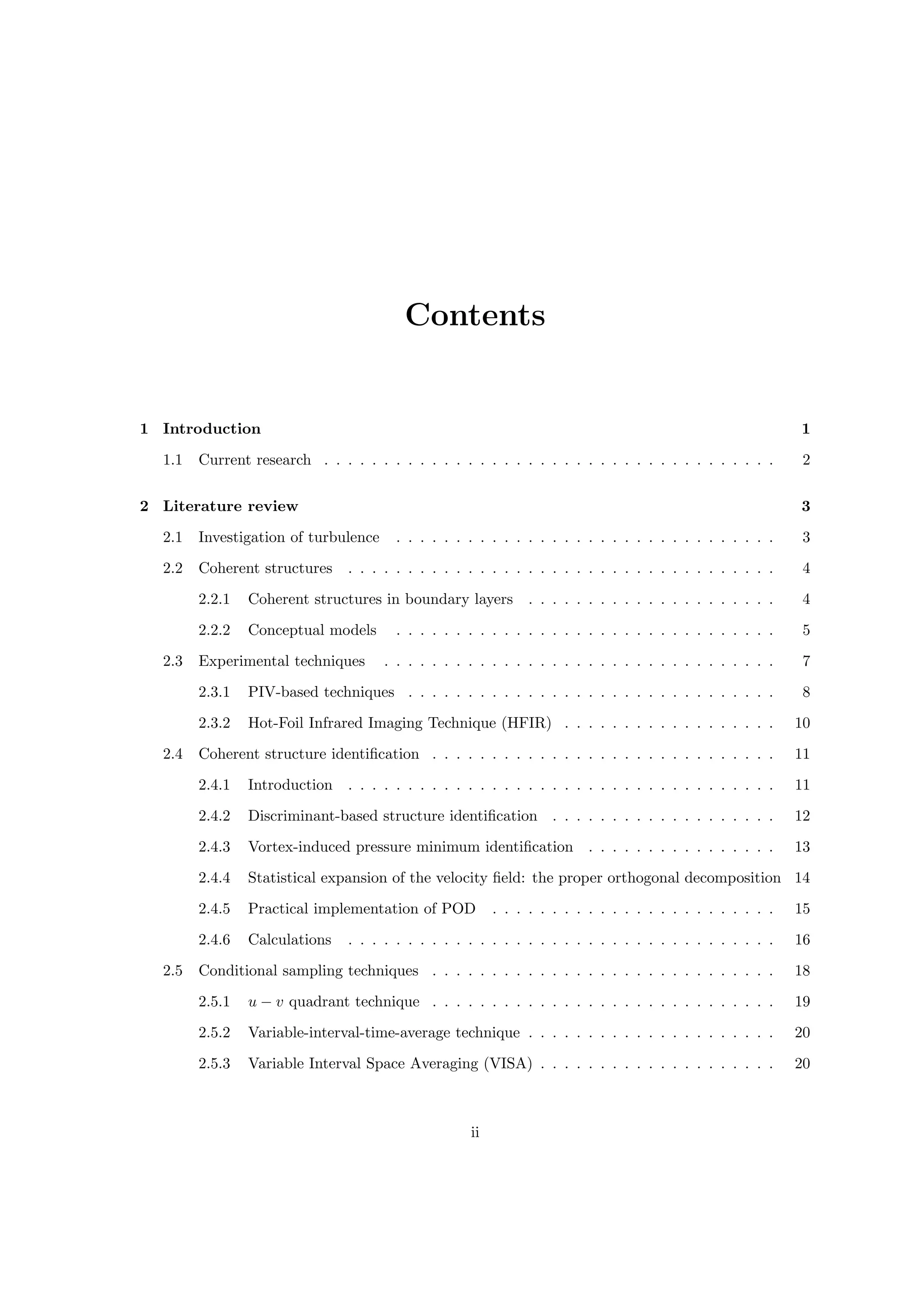
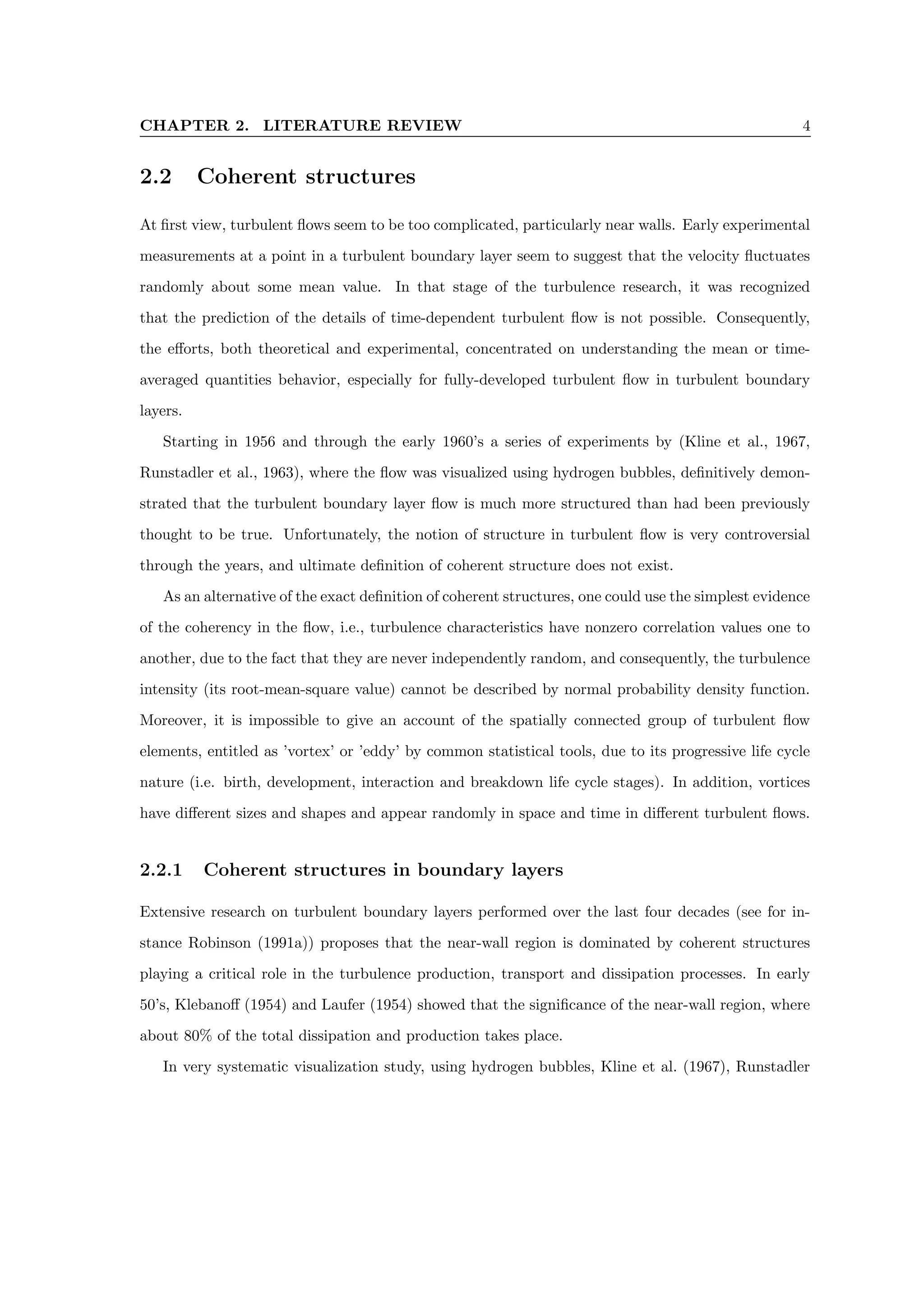
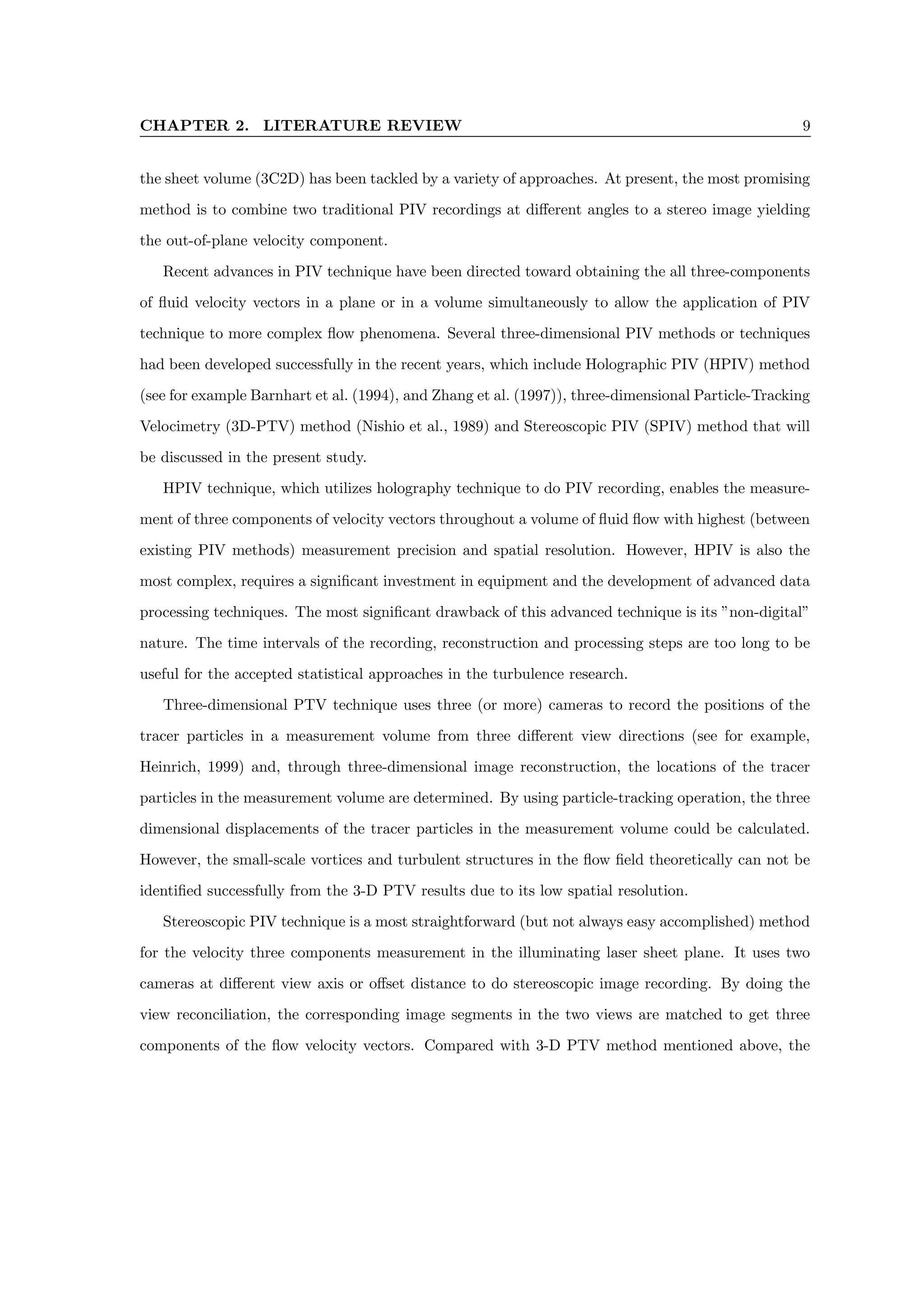
Case No. Plane Coordinates [m] Reh Um [m/s] u∗
[m/s]
1 x − y z = 0.15 21000 0.21 0.011
2 x − y z = 0.15 27000 0.27 0.013
3 x − y z = 0.15 45000 0.45 0.022
4 x − y z = 0.15 57000 0.57 0.027
5 x − z y = 0.003 27000 0.24 0.013
6 x − z y = 0.01 27000 0.24 0.013
7 x − z y = 0.025 27000 0.24 0.013
8 y − z x = 2.50 27000 0.24 0.011
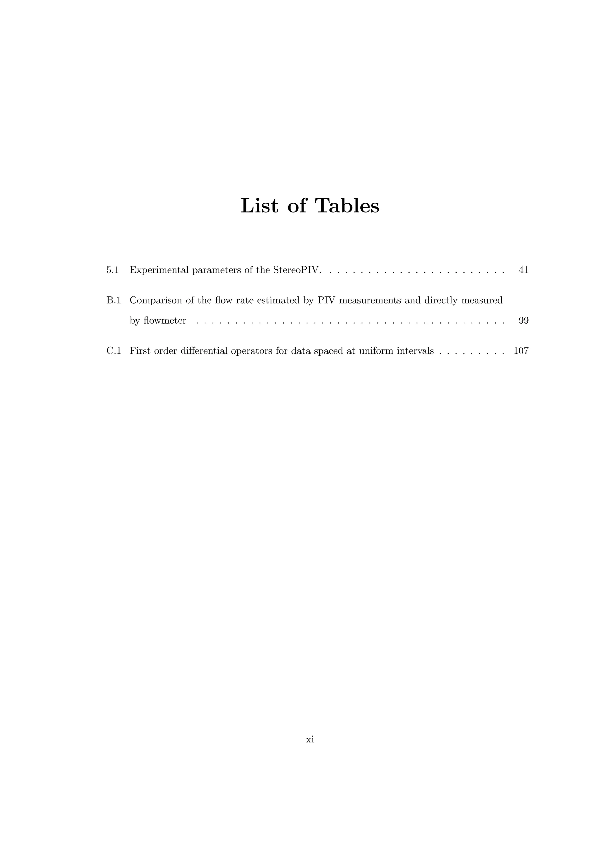
Table 5.1: Experimental parameters of the StereoPIV.
.miieqipd i‘pze mixhnxt :5.1 dlah
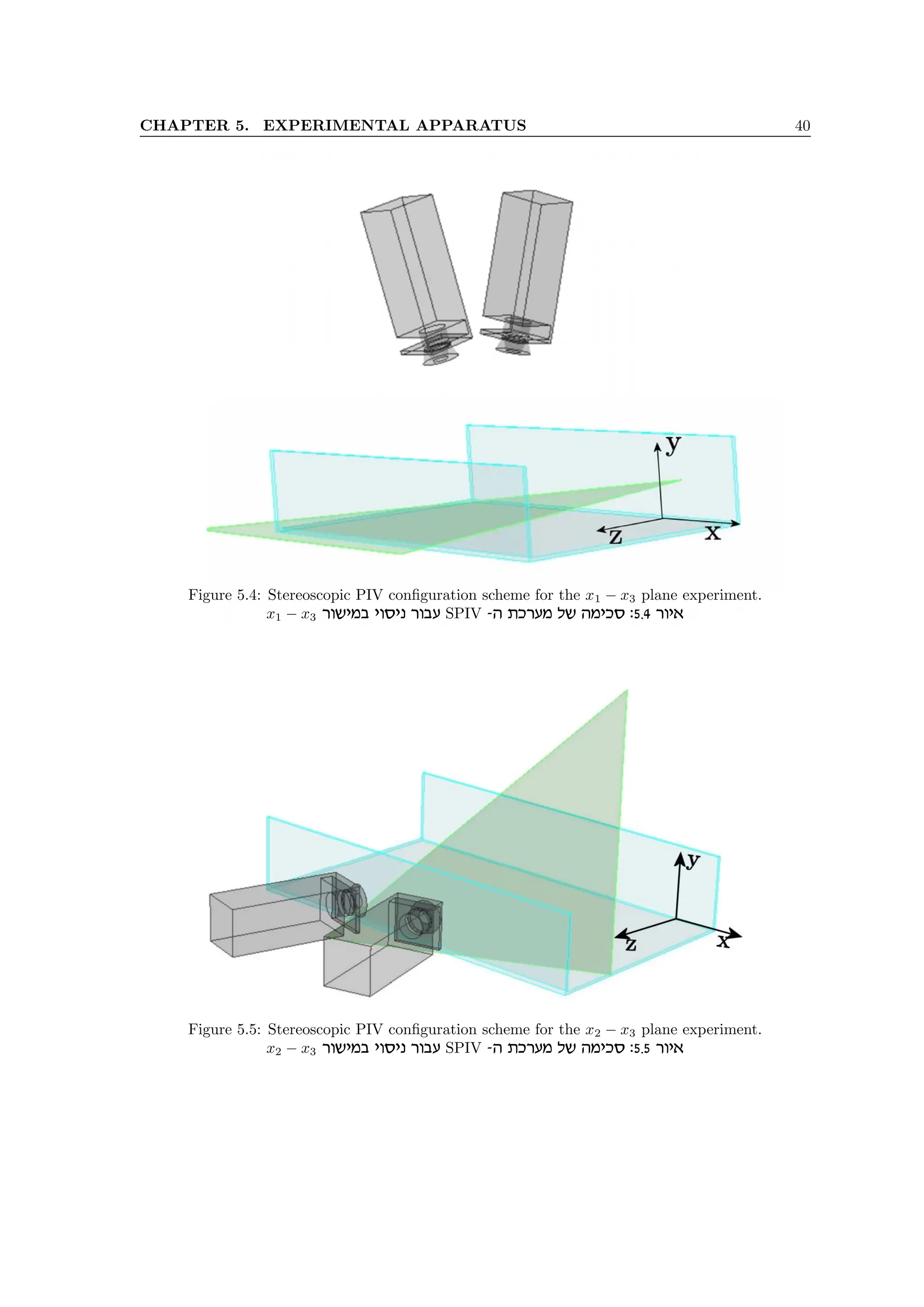
5.4 XPIV – Multi-plane Stereoscopic Particle Image Velocime-
try
In this section, the three dimensional extension of the stereoscopic PIV method, XPIV - Multiplane
SPIV is presented, along with the optical scheme, basic principles and image processing algorithm.
The quality of the velocity data is evaluated by using the velocity profiles, turbulent intensity and
the continuity equation characteristics.
5.4.1 Introduction
Experimental investigation of turbulent flows requires techniques that allow three dimensional mea-
surements with high spatial and temporal resolutions. PIV appears to be an appropriate basis for
three dimensional velocity measurements, as it is presented in the literature review, Section 2.3. The
technique has only technological limitations to achieve a temporal resolution due to the illumination
source (lasers) and recording media (CCD) frequencies which are available today.
Understanding the drawbacks and advantages of the obtainable measurement systems led to
the development of the multi-plane stereoscopic velocimetry technique, XPIV . The technique ap-
plies the principles of multi-sheet illumination, stereoscopic imaging and particle image defocusing.
The experimental technique implemented with a stereoscopic PIV system (Section 5.2), based on
additional optics and image processing algorithm.
Section 5.5 presents the optical configurations implemented during the research. Image processing](https://image.slidesharecdn.com/alexliberzonphdthesisweb-240511095654-b7f38227/75/Coherent-structures-characterization-in-turbulent-flow-53-2048.jpg)


![CHAPTER 6. RESULTS AND DISCUSSION 67
−10 −5 0 5 10 15 20
0.01 0.02 0.03 0.04 0.05 0.06 0.07 0.08 0.09 0.1
0.002
0.007
0.012
0.017
0.022
x [m]
y
[m]
ωz
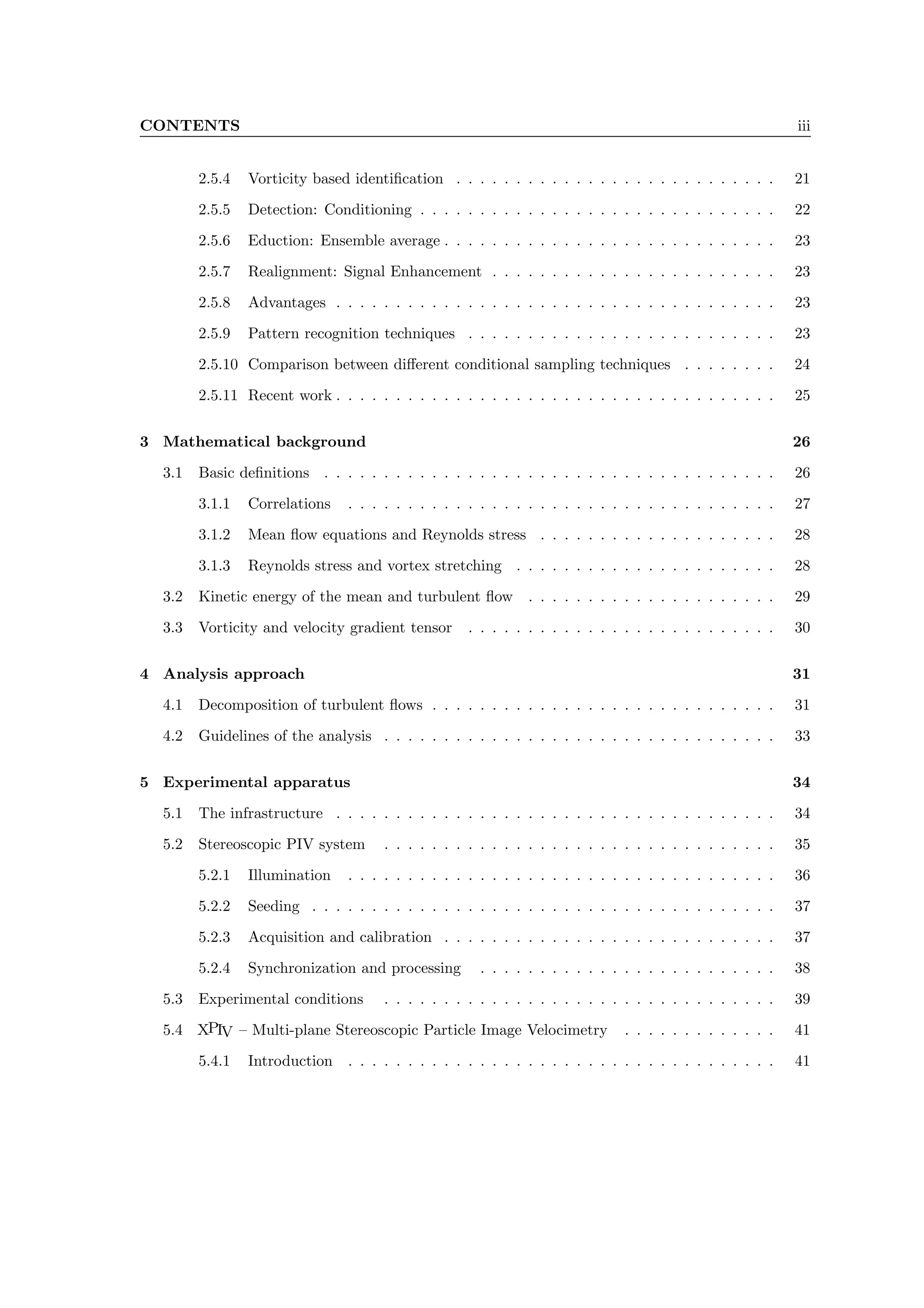
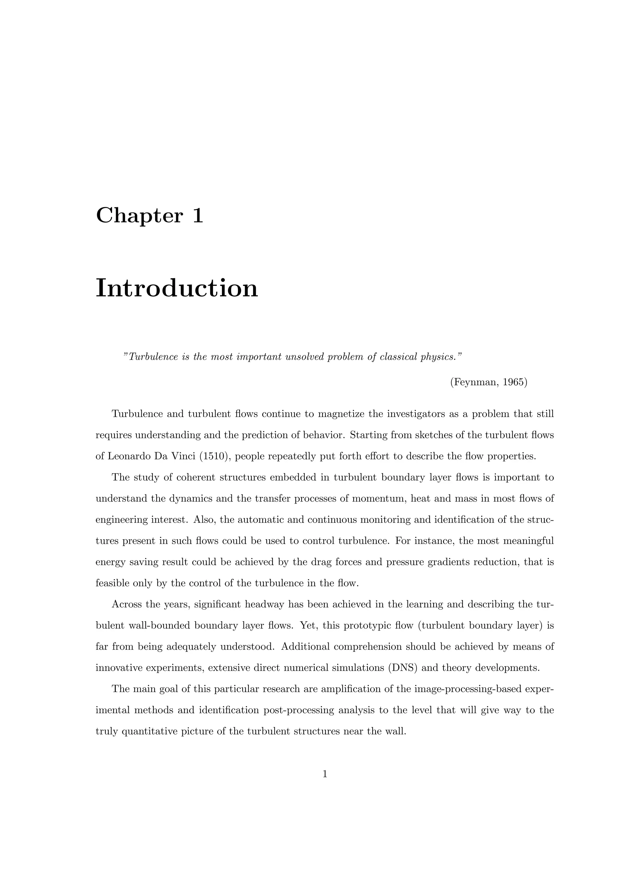
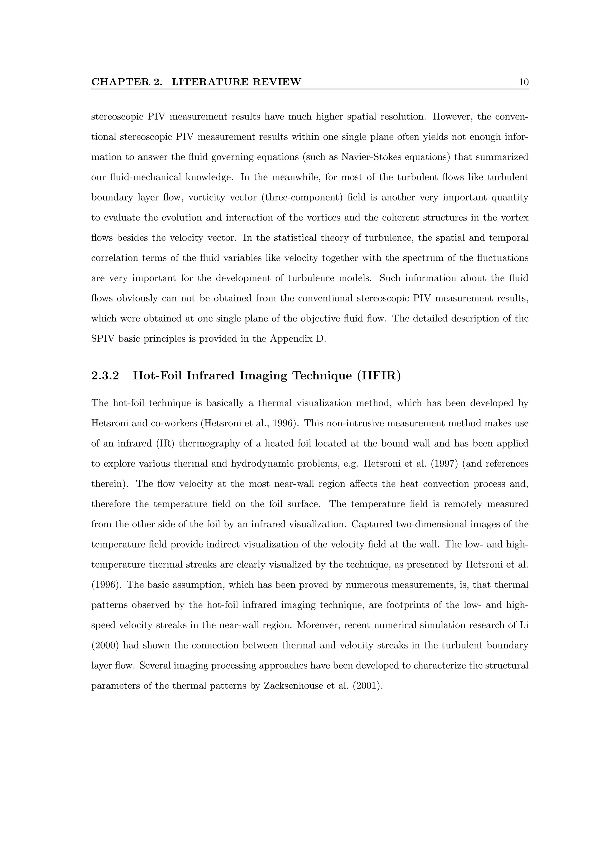
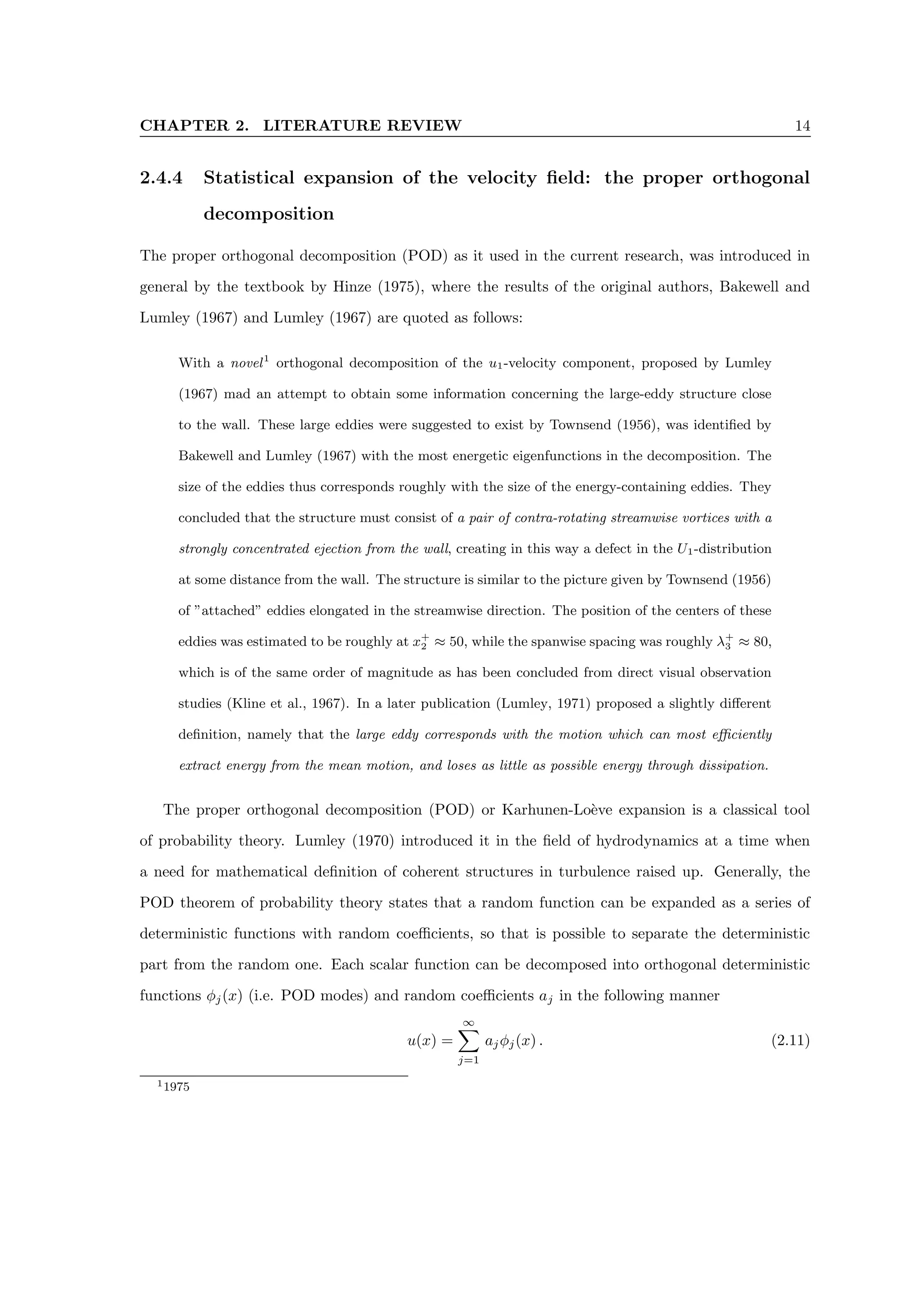
Figure 6.12: Instantaneous vorticity ω3 component field.
.zirbxd zeileaxrd dcy :6.12 xei‘
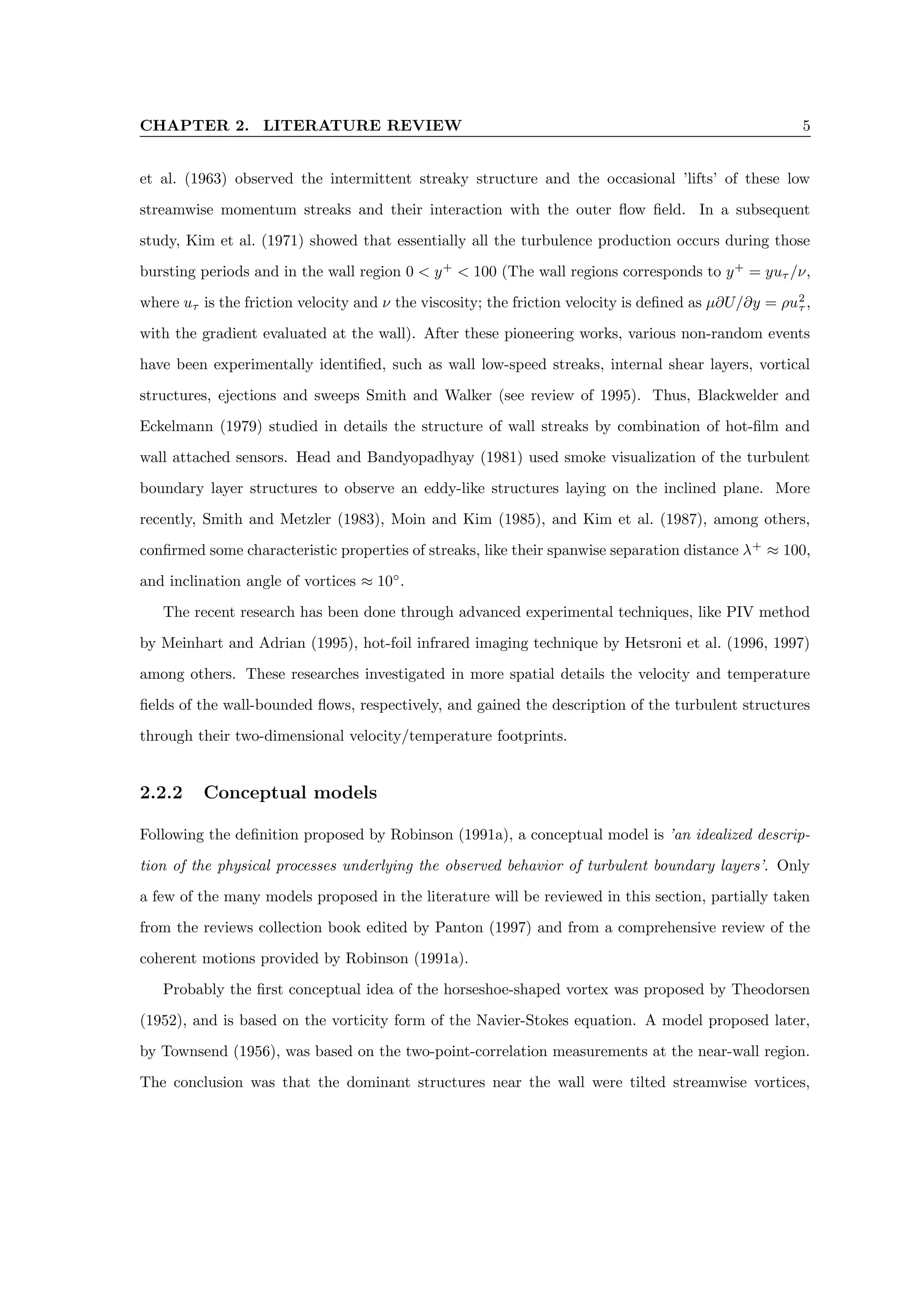
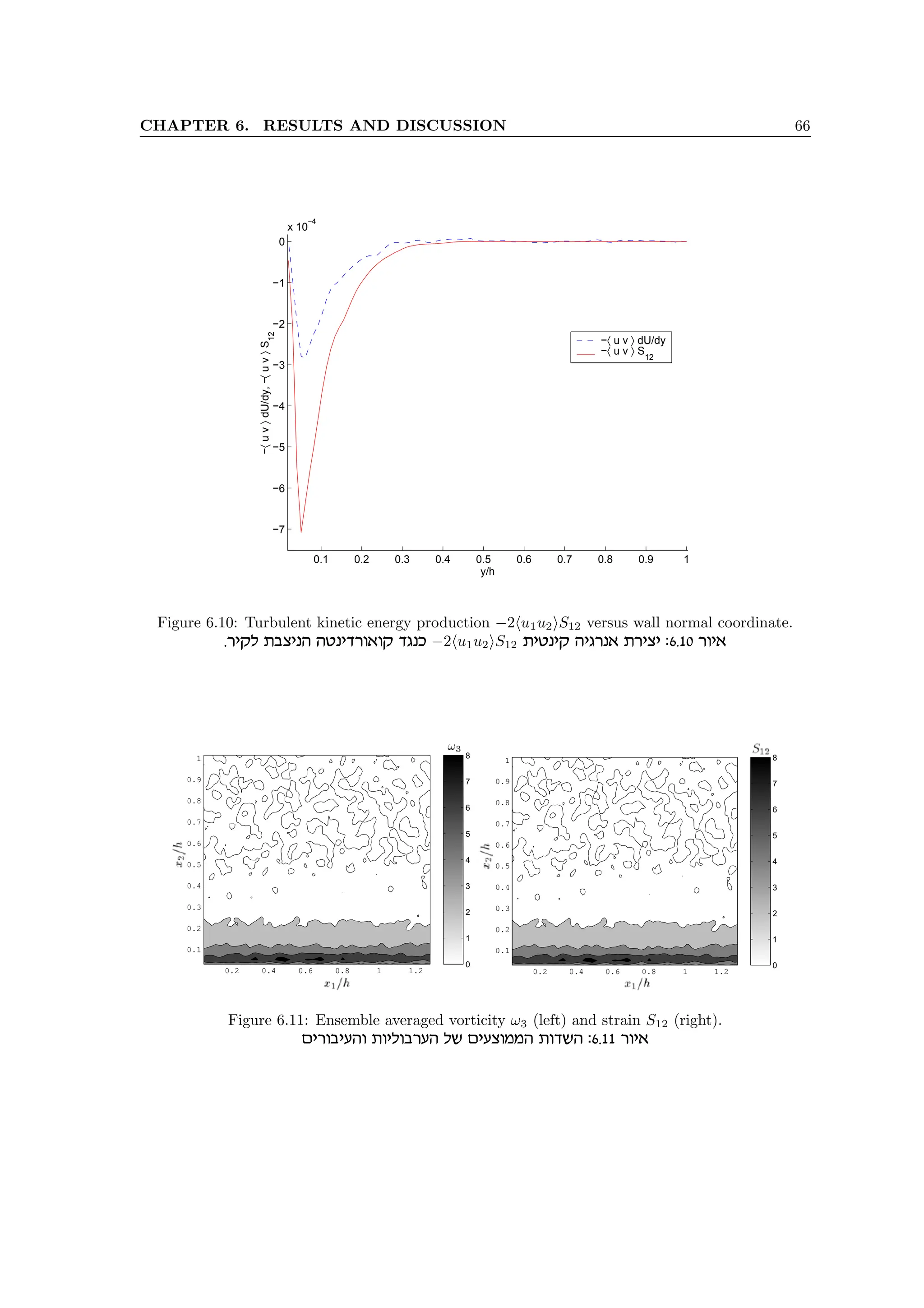
the connection to the turbulent energy production term −hu1u2iS12. Actually, this term represents
the rate at which the energy is transferred from mean flow to turbulent fluctuations. We already
noted that this term appears in the mean flow energy equation (3.16) and proposes that the turbulent
energy is generated from the mean shear. In addition, we present in the following analysis that the
strong mean vorticity (or strain) performs a masking effect on the concealed coherent structure of
the boundary layer. When we look at the instantaneous vorticity fields near the bottom wall, as one
presented in the figure 6.12, we can detect a large region of the concentrated vorticity, elongated in
the streamwise direction and inclined at some small angle (i.e., between 5◦
and 15◦
). Such structures
appear randomly in measured fields and at different streamwise locations, relatively to the measured
flow field boundaries.
6.2 Linear combination of the POD modes
The largest eddies do have directional preferences, and their shapes are characteristic of
the particular mean flow. The recognizable eddies are called ’coherent structures’. The
allusion is to human ability to recognize the forms, rather than to statistical concepts of
coherence. Durbin and Pettersson Reif (2001)](https://image.slidesharecdn.com/alexliberzonphdthesisweb-240511095654-b7f38227/75/Coherent-structures-characterization-in-turbulent-flow-79-2048.jpg)


![CHAPTER 6. RESULTS AND DISCUSSION 89
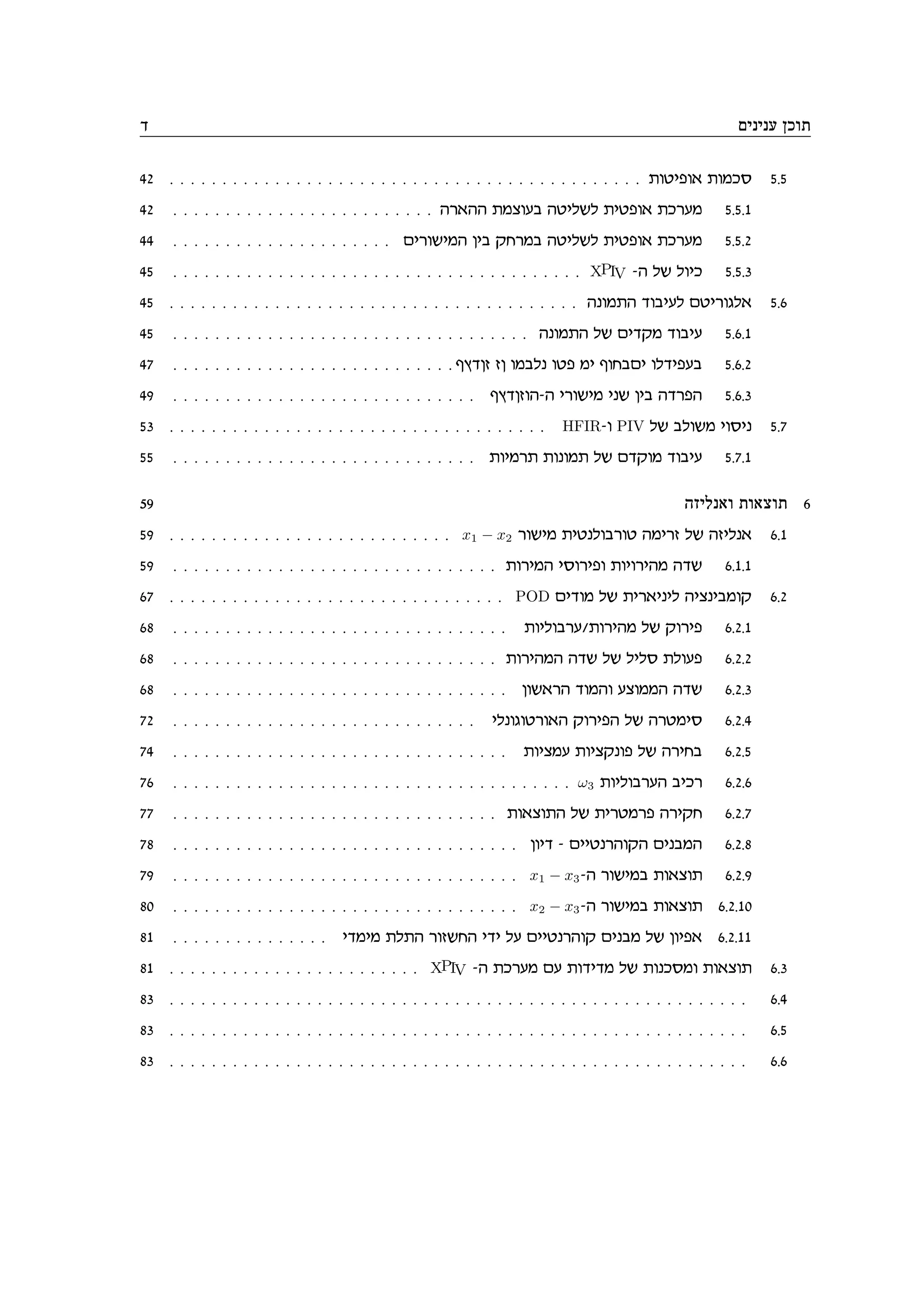
0.2 0.21 0.22 0.23 0.24 0.25 0.26
0.1
0.5
0.9
Figure 6.27: Streamwise velocity average profiles measured by using XPIV (-o) and box-plot of the
PIV measurements in separate y planes(|-[]-|).
.PIV -e XPIV ir cecnd ,dnixfd oeeika zrvennd zexidnd qexit :6.27 xei‘](https://image.slidesharecdn.com/alexliberzonphdthesisweb-240511095654-b7f38227/75/Coherent-structures-characterization-in-turbulent-flow-101-2048.jpg)


![APPENDIX B. PIV VALIDATION 99
Case no. Q (lpm) U∞ [m/s] Qest Error, (%)
1 280 0.20 288 2.8
2 360 0.26 374 3.8
3 525 0.38 547 4.1
Table B.1: Comparison of the flow rate estimated by PIV measurements and directly measured by
flowmeter
.dwitq cn ir dcecne PIV -d ze‘vez jezn zkxreynd dwitqd oia d‘eeyd :a.1 dlah
B.2 Software performance
In order to detect possible bias error inherently introduced by some PIV algorithms, there are
two possible options (i) to analyze standard, synthetically produced images, introduced to the
PIV community by Okamoto et al. (2000), (ii) analyze the real PIV images by different soft-
ware packages. All the PIV measurements, in two dimensional, in stereoscopic and in multiplane
modes are performed by using a commercial software package InsightTM
(Inc., 1999a) that is a
part of the SPIV system. Figure B.1 presents the view of the Insight analysis of the standard
images used in the first-type evaluation analysis. The analysis is performed for the case no. 1
(http://piv.vsj.or.jp/piv/java/image01-e.html) and the evaluation shows an excellent agree-
ment between the known displacement of 7.5 ± 3 pixels and the InsightTM
analysis results in fig-
ure B.1.
The second type evaluation comparison is performed by using the URAPIV, self-made evaluation
software, developed with Matlab r
(http://urapiv.tripod.com). This software allows to analyze
PIV images by using the FFT-based cross-correlation calculation and includes the most common
velocity filters. The advantage of the URAPIV package is its open source and control of all possible
parameters. Figure B.2 depicts a comparison between the results of two software packages. The
graph includes the pixel displacements of the water flow, seeded with hollow glass sphere particles,
and evaluated by using the cross-correlation algorithm. The difference between two results is only
at the level of sub-pixel displacements and is less that 1%.](https://image.slidesharecdn.com/alexliberzonphdthesisweb-240511095654-b7f38227/75/Coherent-structures-characterization-in-turbulent-flow-111-2048.jpg)
![APPENDIX C. DERIVATIVES. PART 1: VORTICITY CALCULATION 118
C.3 Appendix B - Matlabr
procedures
FASTDERIVATIVE.M
function [varargout] = fastderivative(varargin)
%FASTDERIVATIVE Calculates fast derivatives of two-dimensional data
% using 2D convolution (See conv2 for more info).
% [DFDX,DFDY] = FASTDERIVATIVE(F,HX,HY,’METHOD’)
% F - 2D matrix, HX,HY - intervals in X,Y directions.
% ’method’ - one of the following methods:
% ’leastsq’ - 5 points
% ’richardson’ - 5 points
% ’center’ - 3 points, center difference
% ’general’ - default, forward/backward/center in one
% ’5point’ - richardson plus forward/backward on boundaries
%
% [DFDX,DFDY] = FASTDERIVATIVE(F,H,’METHOD’)
% Uses HY = HX = H,
%
% [DFDX,DFDY] = FASTDERIVATIVE(F,’METHOD’)
% Uses default HX,HY = 1.
% Created: 05-Mar-2001
% Author: Alex Liberzon
% E-Mail : liberzon@tx.technion.ac.il
% Phone : +972 (0)48 29 3861
% Copyright (c) 2001 Technion - Israel Institute of Technology
%
% Modified at: 05-Mar-2001
% $Revision: 1.0 $ $Date: 05-Mar-2001 11:59:07$
% Parse inputs
if nargin == 4
[f,hx,hy,method] = deal(varargin{:});
elseif nargin == 3
[f,hx,method] = deal(varargin{:});](https://image.slidesharecdn.com/alexliberzonphdthesisweb-240511095654-b7f38227/75/Coherent-structures-characterization-in-turbulent-flow-130-2048.jpg)
![APPENDIX C. DERIVATIVES. PART 1: VORTICITY CALCULATION 119
hy = hx;
elseif nargin == 2
[f,method] = deal(varargin{:});
hx = 1; hy = 1;
end;
switch lower(method)%
case ’general’,’default’,’3points’,’threepoints’}
dfdx = -conv2([0 1 0],[-1 0 1],f,’same’)/2/hx;
dfdy = -conv2([-1 0 1],[0 1 0],f,’same’)/2/hy;
dfdx(:,1) = f(:,2)-f(:,1);
dfdx(:,end) = -f(:,end-1)+f(:,end);
dfdy(1,:) = f(2,:)-f(1,:);
dfdy(end,:) = -f(end-1,:)+f(end,:);
case {’leastsq’}
dfdx = -conv2([0 0 1 0 0],[-2 -1 0 1 2],f,’valid’)/10/hx;
dfdy = -conv2([-2 -1 0 1 2],[0 0 1 0 0],f,’valid’)/10/hy;
case {’center’}
dfdx = -conv2([0 1 0],[-1 0 1],f,’valid’)/2/hx;
dfdy = -conv2([-1 0 1],[0 1 0],f,’valid’)/2/hy;
case {’richardson’}
dfdx = -conv2([0 0 1 0 0],[1 -8 0 8 -1],f,’valid’)/12/hx;
dfdy = -conv2([1 -8 0 8 -1],[0 0 1 0 0],f,’valid’)/12/hy;
otherwise
error(’Wrong method, see HELP FASTDERIVATIVE ’);
end
varargout{1} = dfdx;%
varargout{2} = dfdy;%
VORTICITY.M
function [varargout] = vorticity(varargin)
%VORTICITY Calculates vorticity and checks the continuity equation.
% [OMEGA,EZZ] = VORTICITY(X,Y,U,V,METHOD)
% returns the vorticity OMEGA and Z-component of the strain EZZ.](https://image.slidesharecdn.com/alexliberzonphdthesisweb-240511095654-b7f38227/75/Coherent-structures-characterization-in-turbulent-flow-131-2048.jpg)
![APPENDIX C. DERIVATIVES. PART 1: VORTICITY CALCULATION 120
%
%
%
% See also FASTDERIVATIVE, PROCS_V4
%
% Created: 02-Mar-2001
% Author: Alex Liberzon
% E-Mail : liberzon@tx.technion.ac.il
% Phone : +972 (0)48 29 3861
% Copyright (c) 2001 Technion - Israel Institute of Technology
%
% Modified at: 05-Mar-2001
% $Revision: 1.02 $ $Date: 05-Mar-2001 23:12:01$
% Inputs:
% The simplest case
[x,y,u,v,method] = deal(varargin{:});
% Parameters:
% Homogeneous grid spacing - the simplest case
DeltaX = max(abs(diff(x(1:2,1))),abs(diff(x(1,1:2))));%
DeltaY = max(abs(diff(y(1:2,1))),abs(diff(y(1,1:2))));%
switch lower(method)%
case {’circulation’,’circ’}
dx=(1/(8*DeltaX)).*...
[-1 0 1
-2 0 2
-1 0 1];
dy=(1/(8*DeltaY)).*...
[-1 -2 -1
0 0 0
1 2 1];
vort = - conv2(v,dx,’valid’) + conv2(u,dy,’valid’);
dvdy = conv2(v,dx,’valid’);](https://image.slidesharecdn.com/alexliberzonphdthesisweb-240511095654-b7f38227/75/Coherent-structures-characterization-in-turbulent-flow-132-2048.jpg)
![APPENDIX C. DERIVATIVES. PART 1: VORTICITY CALCULATION 121
dudx = conv2(u,dy,’valid’);
cont = dudx + dvdy;
case {’richardson’}
[dudx,dudy] = fastderivative(u,DeltaX,DeltaY,’richardson’);
[dvdx,dvdy] = fastderivative(v,DeltaX,DeltaY,’richardson’);
vort = dvdx - dudy;
cont = dudx + dvdy;
case {’leastsquares’,’leastsq’}
[dudx,dudy] = fastderivative(u,DeltaX,DeltaY,’leastsq’);
[dvdx,dvdy] = fastderivative(v,DeltaX,DeltaY,’leastsq’);
vort = dvdx - dudy;
cont = dudx + dvdy;
case {’center’}
[dudx,dudy] = fastderivative(u,DeltaX,DeltaY,’center’);
[dvdx,dvdy] = fastderivative(v,DeltaX,DeltaY,’center’);
vort = dvdx - dudy;
cont = dudx + dvdy;
otherwise
disp(’Wrong method’);
end
varargout{1} = vort; varargout{2} = cont;
Simulation procedure: PROCS V4.M
clear all%
[x,y,u,v,vort,dU] = vortex_flow(1,1,1,0);%
indx = 0; indy = 0;
for N = [100,500,1000]
indx = indx + 1;
indy = 0;
for errorlevel = [0.02 0.05 0.075]
indy = indy + 1;
U = zeros([size(u),N]);
V = zeros([size(u),N]);](https://image.slidesharecdn.com/alexliberzonphdthesisweb-240511095654-b7f38227/75/Coherent-structures-characterization-in-turbulent-flow-133-2048.jpg)
![APPENDIX C. DERIVATIVES. PART 1: VORTICITY CALCULATION 122
% Monte Carlo:
for i = 1:N,
U(:,:,i) = u + normrnd(0,errorlevel*max(u(:))/1.96,[size(u)]);
end
for i = 1:N,
V(:,:,i) = v + normrnd(0,errorlevel*max(v(:))/1.96,[size(v)]);
end
[omegar,contr,omegal,contl] = deal(zeros(47,47,N));
[omegac,contc,omega3,cont3] = deal(zeros(49,49,N));
for i = 1:N,
[omegar(:,:,i),contr(:,:,i)] = vorticity_v4(x,y,U(:,:,i),V(:,:,i),’richardson’);
[omega3(:,:,i),cont3(:,:,i)] = vorticity_v4(x,y,U(:,:,i),V(:,:,i),’center’);
[omegal(:,:,i),contl(:,:,i)] = vorticity_v4(x,y,U(:,:,i),V(:,:,i),’leastsq’);
[omegac(:,:,i),contc(:,:,i)] = vorticity_v4(x,y,U(:,:,i),V(:,:,i),’circulation’);%
end;
% End of calculations
% Relative error = (mean(omegaI(:,:,i),3) - vort)/rms(vort);
relerror3(indx,indy) = rms((mean(omega3,3)-vort(2:end-1,2:end-1))/...
rms(vort(2:end-1,2:end-1)));
relerrorc(indx,indy) = rms((mean(omegac,3)-vort(2:end-1,2:end-1))/...
rms(vort(2:end-1,2:end-1)));
relerrorr(indx,indy) = rms((mean(omegar,3)-vort(3:end-2,3:end-2))/...
rms(vort(3:end-2,3:end-2)));
relerrorl(indx,indy) = rms((mean(omegal,3)-vort(3:end-2,3:end-2))/...
rms(vort(3:end-2,3:end-2)));
end% End of errorlevel loop
end% End of N loop
% Continuity check
figure,subplot(221),
pcolor(mean(cont3,3)),shading interp, colorbar horiz
title(’3 point, center difference’);
subplot(222),pcolor(mean(contr,3)),shading interp, colorbar horiz](https://image.slidesharecdn.com/alexliberzonphdthesisweb-240511095654-b7f38227/75/Coherent-structures-characterization-in-turbulent-flow-134-2048.jpg)
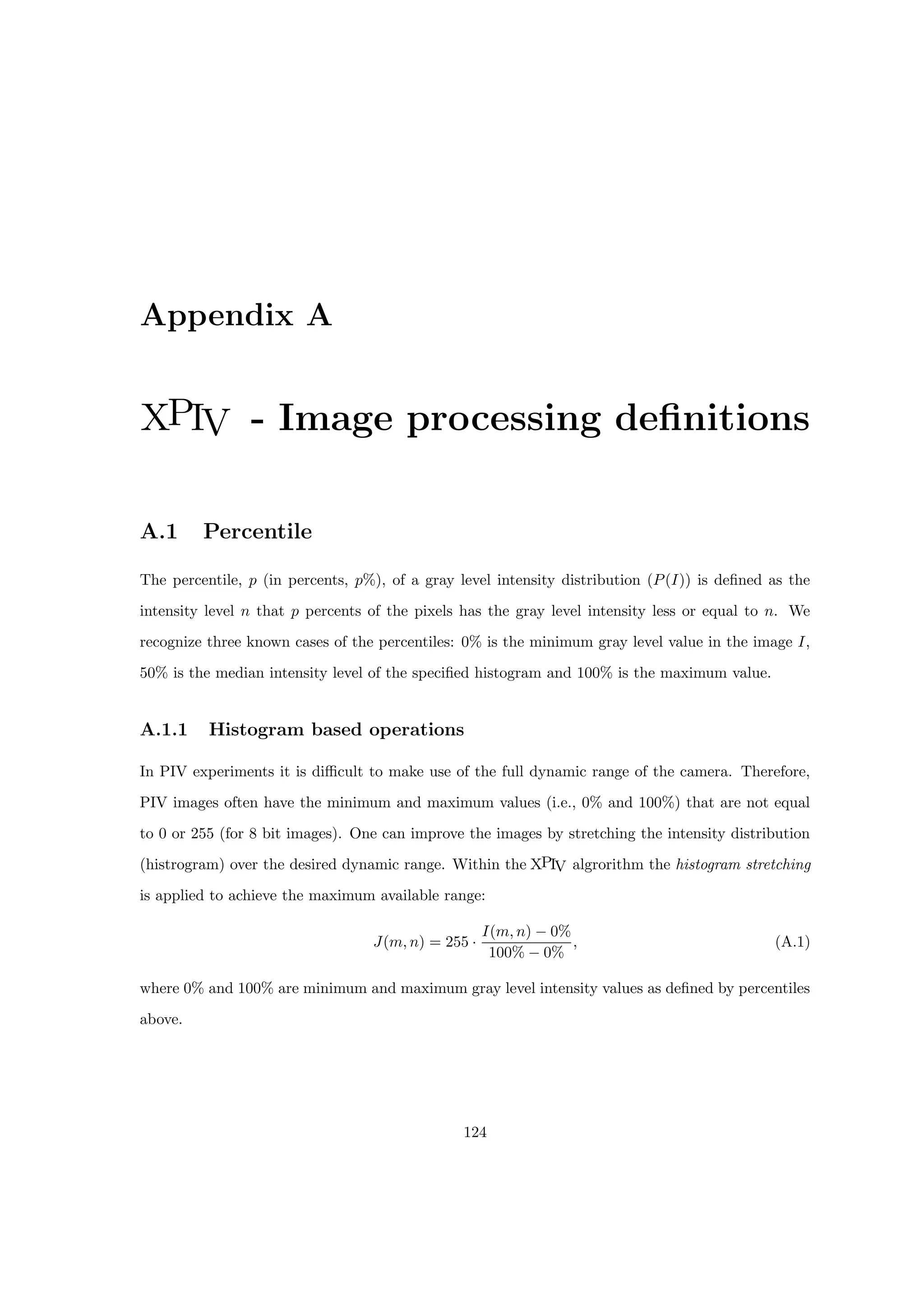
![APPENDIX A. XPIV - IMAGE PROCESSING DEFINITIONS 125
A.1.2 Derivative based operations
Since digital image processing techniques deal with discrete digitized images presented over the
rectangular grid, I(m, n), the derivative based operations lie on the derivative approximations. Thus
the image gradient ∇I is approximated by the sum of two convolutions in row-wise and column-wise
directions, denoted as x and y, respectively:
∇I = (hx ⊗ I)x + (hy ⊗ I)y
where subscripts x and y denote the projections on the x or y axis. Thus, the gradient magnitude
is defined as:
Ig =
q
(hx ⊗ I)
2
+ (hy ⊗ I)
2
.
There are many possible operators for hx and hy and most simple ones are [1 − 1] or [1 0 − 1] as
hx and their transposes, hy = ht
x.
A.2 Morphology based operations
In morphology based operations, we refer to the image (either binary or intensity level) as a set of
objects and background (Serra, 1982, Giardina, 1988):
I = {x |I(x) ⊂ Y }
where Y is the set under R2
that satisfies some predefined property. For example, for the binary
image of 0’s and 1’s, objects are all pixels that are equal to 1, i.e. I = {x |I(x) = 1}. The background
or in other definition, complement of I is defined as all elements that are not in set of I:
Ic
= {x |x /
∈ I}
Each object can be treated by one of four basic operators: union ∪, intersection ∩, complement c
and translation, which is defined for set I and vector b as:
I + b = {x + b |x ∈ I}
or in other words, all pixels that are covered by set I (an object) by shifting, as it is defined in vector
b.
Two basic mathematical morphology operations for binary sets {0, 1} are defined as following:](https://image.slidesharecdn.com/alexliberzonphdthesisweb-240511095654-b7f38227/75/Coherent-structures-characterization-in-turbulent-flow-137-2048.jpg)
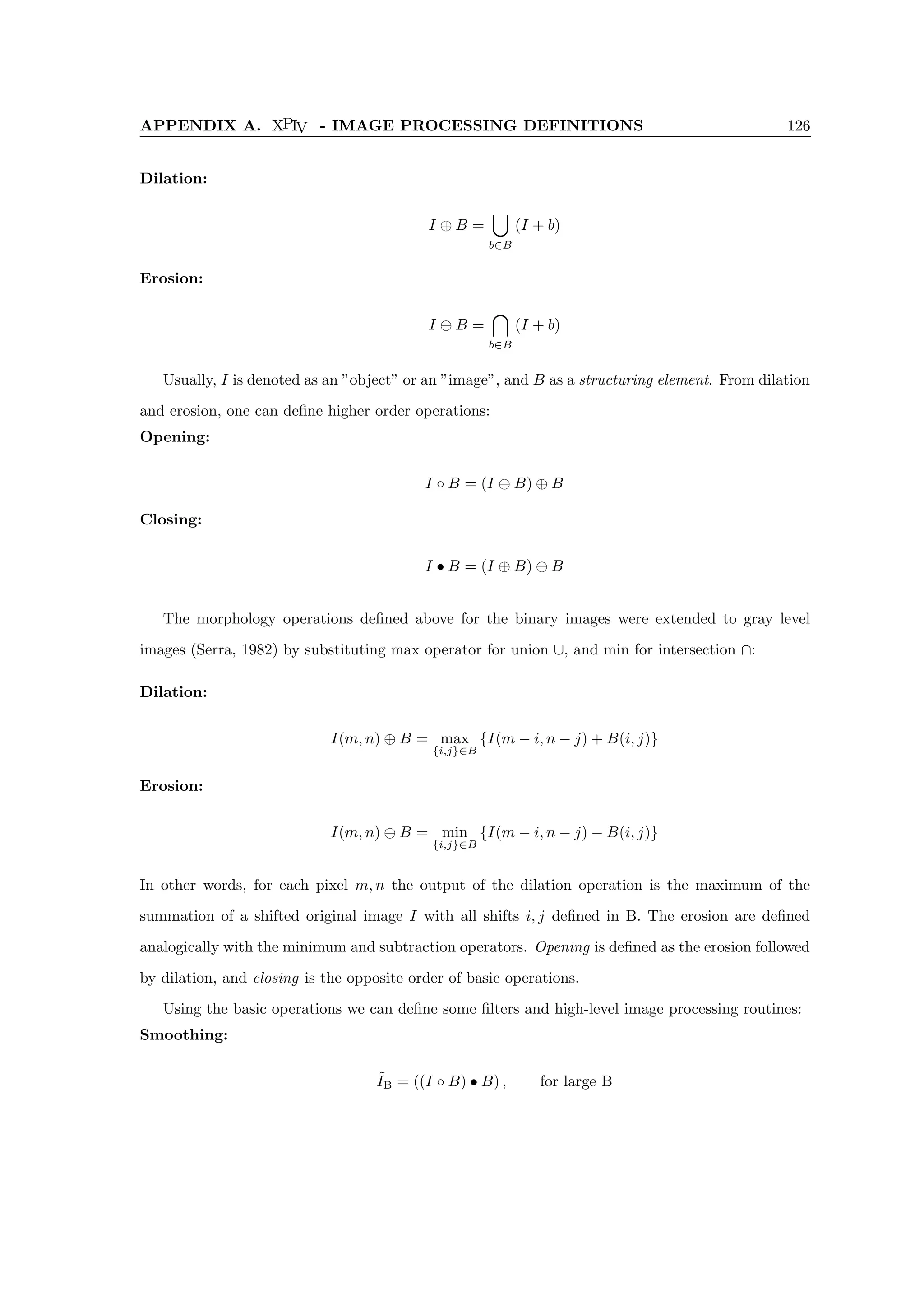
![APPENDIX A. XPIV - IMAGE PROCESSING DEFINITIONS 127
Gradient:
Ig =
1
2
((I ⊕ B) − (I B))
Laplacian:
∇2
= IL =
1
2
[((I ⊕ B) − I) − (I − (I B))] =
=
1
2
((I ⊕ B) + (I B) − 2I)
Background correction:
ˆ
IB = I − ˜
IB
A.3 Segmentation
Segmentation is one of the most common operations in high-level image processing and computer
vision. The target is to distinguish between the ”objects” and the ”background” and the most
popular techniques are thresholding and edge detection.
Thresholding:
IT = {x |I(x) ≥ T}
where T is the threshold. The threshold can be defined arbitrarily or by using one of the
common techniques defined on the histogram of the image. The isodata algorithm, for example,
is an iterative technique (Ridler and Calvard, 1978), where histogram is divided into two groups
by its mean value, and in the following iterations the threshold is defined as the average of
two mean values of each group, until the difference is insignificant. Another common and
fast technique is entitled background symmetry algorithm. This algorithm is based on the
assumption that the maximum peak within the histogram is of the background and uses
percentiles to define the limits of the background population. Then, using the symmetry
assumption, the threshold is defined as:
T = max {P(I)} − (p% − max {P(I)}) .](https://image.slidesharecdn.com/alexliberzonphdthesisweb-240511095654-b7f38227/75/Coherent-structures-characterization-in-turbulent-flow-139-2048.jpg)
![APPENDIX B. SURFACTANTS 133
0.03
0.035
0.04
0.045
0.05
0.055
0.06
0.065
0.07
0.075
0.08
−20 −10 0 10 20 30
−40
−30
−20
−10
0
10
20
30
Z [mm]
X
[mm]
0.03
0.035
0.04
0.045
0.05
0.055
0.06
0.065
0.07
0.075
0.08
−20 −10 0 10 20 30
−40
−30
−20
−10
0
10
20
30
Z [mm]
X
[mm]
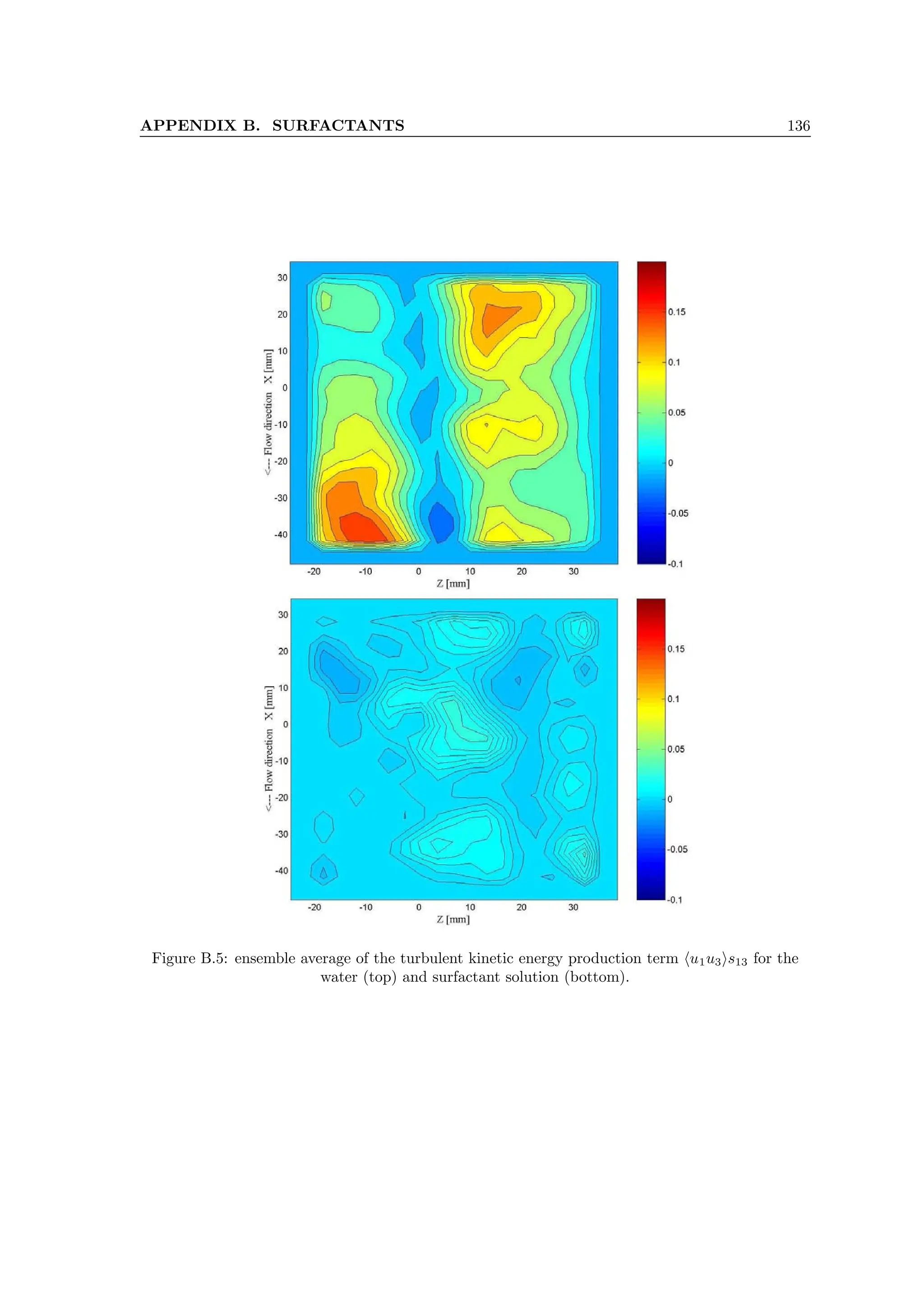
Figure B.2: ensemble average of the turbulent intensity
p
hu2
1i/uq for the water (top) and
surfactant solution (bottom).](https://image.slidesharecdn.com/alexliberzonphdthesisweb-240511095654-b7f38227/75/Coherent-structures-characterization-in-turbulent-flow-145-2048.jpg)
![APPENDIX B. SURFACTANTS 134
−0.08
−0.06
−0.04
−0.02
0
0.02
0.04
−20 −10 0 10 20 30
−40
−30
−20
−10
0
10
20
30
Z [mm]
X
[mm]
−0.08
−0.06
−0.04
−0.02
0
0.02
0.04
−20 −10 0 10 20 30
−40
−30
−20
−10
0
10
20
30
Z [mm]
X
[mm]
Figure B.3: ensemble average of the one-point correlation between streamwise and spanwise
velocity fluctuations hu1u3i for the water (top) and surfactant solution (bottom).](https://image.slidesharecdn.com/alexliberzonphdthesisweb-240511095654-b7f38227/75/Coherent-structures-characterization-in-turbulent-flow-146-2048.jpg)
![APPENDIX B. SURFACTANTS 135
−25 −20 −15 −10 −5 0 5 10 15 20 25
−4
−3
−2
−1
0
1
2
3
4
5
x 10
−4
Z [mm]
Reynolds
stress
〈u
1
u
3
〉
Water
Agrimul 20 ppm
Figure B.4: streamwise average of the hu1u3i correlation for the water (solid line) and surfactant
solution (star-marked line).](https://image.slidesharecdn.com/alexliberzonphdthesisweb-240511095654-b7f38227/75/Coherent-structures-characterization-in-turbulent-flow-147-2048.jpg)