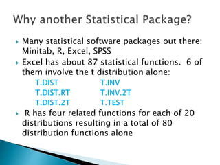
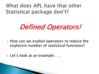
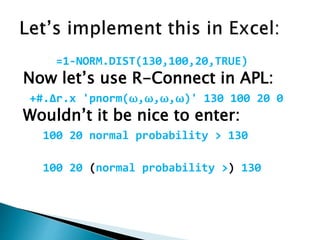
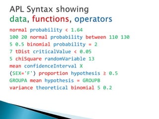
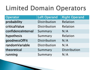
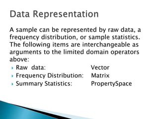
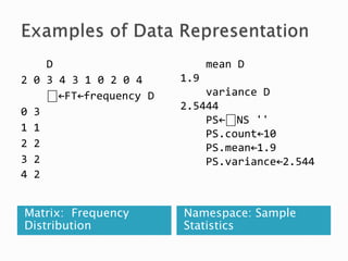
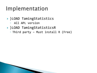
Stephen Mansour, PhD
University of Scranton and The Carlisle Group
Dyalog ’14 Conference, Eastbourne, UK
 Many statistical software packages out there:
Minitab, R, Excel, SPSS
 Excel has about 87 statistical functions. 6 of
them involve the t distribution alone:
T.DIST T.INV
T.DIST.RT T.INV.2T
T.DIST.2T T.TEST
 R has four related functions for each of 20
distributions resulting in a total of 80
distribution functions alone
Defined Operators!
 How can we exploit operators to reduce the
explosive number of statistical functions?
 Let’s look at an example . . .
 Typical attendance is about 100 delegates
with a standard deviation of 20.
 Assume next year’s conference centre can
support up to130 delegates.
 What are the chances that next year’s
attendance will exceed capacity?
=1-NORM.DIST(130,100,20,TRUE)
Now let’s use R-Connect in APL:
+#.∆r.x 'pnorm(⍵,⍵,⍵,⍵)' 130 100 20 0
Wouldn’t it be nice to enter:
100 20 normal probability > 130
100 20 (normal probability >) 130
normal probability < 1.64
100 20 normal probability between 110 130
5 0.5 binomial probability = 2
7 tDist criticalValue < 0.05
5 chiSquare randomVariable 13
mean confidenceInterval X
(SEX='F') proportion hypothesis ≥ 0.5
GROUPA mean hypothesis = GROUPB
variance theoretical binomial 5 0.2
 Summary Functions
◦ Descriptive Statistics
 Probability Distributions
◦ Theoretical Models
 Relations
 Summary functions are of the form:
𝑦 = 𝑓 𝑥1, 𝑥2, … 𝑥 𝑛
 They produce a single value from a vector.
 Structurally they are equivalent to g/ where g is a
scalar function and the right argument is a simple
numeric vector.
 A statistic is a summary function of a sample; a
parameter is a summary function of a population.
 Examples
◦ Measures of central tendency:
mean, median, mode
◦ Measures of Spread
variance, standard deviation, range , IQR
◦ Measures of Position
min, max, quartiles, percentiles
◦ Measures of shape
skewness, kurtosis
 Probability Distributions are functions defined
in a natural way when they are called without
an operator:
◦ Discrete: probability mass function
◦ Continuous: density function
 Left argument is parameter list
 Right argument can be any value taken on by
the distribution.
 Probability Distributions are scalar with
respect to the right argument.
Discrete
Distributions
Parameter List
uniform a - lower bound (default 1), b - upper bound.
binomial n - Sample size, p - probability of success
poisson λ - average number of arrivals per time period
negativeBinomial n - number of success, p - probability of success
hyperGeometric m - number of successes , n - sample size ,
N - Population size
multinomial V - List of Values (default 1 thru n),
P - List of probabilities totaling 1
Continuous Distributions Parameter List
normal μ - theoretical mean (default 0); σ - standard deviation
(default 1)
exponential λ - mean time to fail
rectangular (continuous
uniform)
a - lower bound (default 0), b - upper bound (default 1)
triangular a - lower bound, m - most common value,
b - upper bound
chiSquare df - degrees of freedom
tDist (Student) df - degrees of freedom
fDist df1 - degrees of freedom for numerator,
df2 - degrees of freedom for denominator
 Relational functions are dyadic functions
whose range is {0,1}
 1=relation is satisfied, 0 otherwise.
 Examples:
< ≤ = ≥ > ≠ ∊
between←{¯1=×/×⍺∘.-⍵}
 By limiting the domain of an operator to one
of the previously-defined functional
classifications, we can create an operator to
perform statistical analysis.
 For a dyadic operator, each operand can be
limited to a particular (but not necessarily the
same) functional classification.
Operator Left Operand Right Operand
probability Distribution Relation
criticalValue Distribution Relation
confidenceInterval Summary N/A
hypothesis Summary Relation
goodnessOfFit Distribution N/A
randomVariable Distribution N/A
theoretical Summary Distribution
running Summary N/A
 Most functions and operators can easily be
written in APL.
 Internals not important to user
 R interface can be used if necessary for
statistical distributions.
 Correct nomenclature and ease of use is
critical.
A sample can be represented by raw data, a
frequency distribution, or sample statistics.
The following items are interchangeable as
arguments to the limited domain operators
above:
 Raw data: Vector
 Frequency Distribution: Matrix
 Summary Statistics: PropertySpace
Matrix: Frequency
Distribution
Namespace: Sample
Statistics
D
2 0 3 4 3 1 0 2 0 4
⎕←FT←frequency D
0 3
1 1
2 2
3 2
4 2
mean D
1.9
variance D
2.5444
PS←⎕NS ''
PS.count←10
PS.mean←1.9
PS.variance←2.544
 )LOAD TamingStatistics
◦ All APL version
 )LOAD TamingStatisticsR
◦ Third party – Must install R (Free)
 There are many statistical packages out there;
some, like R can be used with APL
 Operator syntax is unique to APL
 R can be called directly from APL using
RCONNECT, but APL operator syntax is easier
to understand.

TamingStatistics

  • 1.
    Stephen Mansour, PhD Universityof Scranton and The Carlisle Group Dyalog ’14 Conference, Eastbourne, UK
  • 2.
     Many statisticalsoftware packages out there: Minitab, R, Excel, SPSS  Excel has about 87 statistical functions. 6 of them involve the t distribution alone: T.DIST T.INV T.DIST.RT T.INV.2T T.DIST.2T T.TEST  R has four related functions for each of 20 distributions resulting in a total of 80 distribution functions alone
  • 3.
    Defined Operators!  Howcan we exploit operators to reduce the explosive number of statistical functions?  Let’s look at an example . . .
  • 4.
     Typical attendanceis about 100 delegates with a standard deviation of 20.  Assume next year’s conference centre can support up to130 delegates.  What are the chances that next year’s attendance will exceed capacity?
  • 5.
    =1-NORM.DIST(130,100,20,TRUE) Now let’s useR-Connect in APL: +#.∆r.x 'pnorm(⍵,⍵,⍵,⍵)' 130 100 20 0 Wouldn’t it be nice to enter: 100 20 normal probability > 130 100 20 (normal probability >) 130
  • 6.
    normal probability <1.64 100 20 normal probability between 110 130 5 0.5 binomial probability = 2 7 tDist criticalValue < 0.05 5 chiSquare randomVariable 13 mean confidenceInterval X (SEX='F') proportion hypothesis ≥ 0.5 GROUPA mean hypothesis = GROUPB variance theoretical binomial 5 0.2
  • 7.
     Summary Functions ◦Descriptive Statistics  Probability Distributions ◦ Theoretical Models  Relations
  • 8.
     Summary functionsare of the form: 𝑦 = 𝑓 𝑥1, 𝑥2, … 𝑥 𝑛  They produce a single value from a vector.  Structurally they are equivalent to g/ where g is a scalar function and the right argument is a simple numeric vector.  A statistic is a summary function of a sample; a parameter is a summary function of a population.
  • 9.
     Examples ◦ Measuresof central tendency: mean, median, mode ◦ Measures of Spread variance, standard deviation, range , IQR ◦ Measures of Position min, max, quartiles, percentiles ◦ Measures of shape skewness, kurtosis
  • 10.
     Probability Distributionsare functions defined in a natural way when they are called without an operator: ◦ Discrete: probability mass function ◦ Continuous: density function  Left argument is parameter list  Right argument can be any value taken on by the distribution.  Probability Distributions are scalar with respect to the right argument.
  • 11.
    Discrete Distributions Parameter List uniform a- lower bound (default 1), b - upper bound. binomial n - Sample size, p - probability of success poisson λ - average number of arrivals per time period negativeBinomial n - number of success, p - probability of success hyperGeometric m - number of successes , n - sample size , N - Population size multinomial V - List of Values (default 1 thru n), P - List of probabilities totaling 1
  • 12.
    Continuous Distributions ParameterList normal μ - theoretical mean (default 0); σ - standard deviation (default 1) exponential λ - mean time to fail rectangular (continuous uniform) a - lower bound (default 0), b - upper bound (default 1) triangular a - lower bound, m - most common value, b - upper bound chiSquare df - degrees of freedom tDist (Student) df - degrees of freedom fDist df1 - degrees of freedom for numerator, df2 - degrees of freedom for denominator
  • 13.
     Relational functionsare dyadic functions whose range is {0,1}  1=relation is satisfied, 0 otherwise.  Examples: < ≤ = ≥ > ≠ ∊ between←{¯1=×/×⍺∘.-⍵}
  • 14.
     By limitingthe domain of an operator to one of the previously-defined functional classifications, we can create an operator to perform statistical analysis.  For a dyadic operator, each operand can be limited to a particular (but not necessarily the same) functional classification.
  • 15.
    Operator Left OperandRight Operand probability Distribution Relation criticalValue Distribution Relation confidenceInterval Summary N/A hypothesis Summary Relation goodnessOfFit Distribution N/A randomVariable Distribution N/A theoretical Summary Distribution running Summary N/A
  • 16.
     Most functionsand operators can easily be written in APL.  Internals not important to user  R interface can be used if necessary for statistical distributions.  Correct nomenclature and ease of use is critical.
  • 17.
    A sample canbe represented by raw data, a frequency distribution, or sample statistics. The following items are interchangeable as arguments to the limited domain operators above:  Raw data: Vector  Frequency Distribution: Matrix  Summary Statistics: PropertySpace
  • 18.
    Matrix: Frequency Distribution Namespace: Sample Statistics D 20 3 4 3 1 0 2 0 4 ⎕←FT←frequency D 0 3 1 1 2 2 3 2 4 2 mean D 1.9 variance D 2.5444 PS←⎕NS '' PS.count←10 PS.mean←1.9 PS.variance←2.544
  • 19.
     )LOAD TamingStatistics ◦All APL version  )LOAD TamingStatisticsR ◦ Third party – Must install R (Free)
  • 20.
     There aremany statistical packages out there; some, like R can be used with APL  Operator syntax is unique to APL  R can be called directly from APL using RCONNECT, but APL operator syntax is easier to understand.