data science important material..........

21AD62
JOIN WHATSAPP CHANNEL
OR GROUP
01082024
US
N
Model Question Paper-1/2 with effect from 2021(CBCS Scheme)
Sixth Semester B.E. Degree Examination Data
science and its applications (21AD62)
TIME: 03 Hours Max. Marks:
100
Note: 01. 02. Answer any FIVE full questions, choosing at least ONE question from
each module THESE ANSWERS FROM TEXTBOOK
Module -1
(download)
Bloom’s
Taxono
my
Level
COs
Mark
s
Q.01 a
What is data Visualization? Explain bar chart and line
chart
Data Visualization: Understanding Bar Charts and Line
Charts
What is Data Visualization?
Data visualization is a powerful tool used to explore and
communicate data effectively. It involves creating visual
representations of data to identify patterns, trends, and
relationships within datasets. Two primary uses of data
visualization are to explore data and to communicate data
insights to others.
Bar Charts
- Definition : A bar chart is ideal for showing how a
quantity varies among a discrete set of items.
- Example : A simple bar chart can display how many
Academy Awards were won by different movies.
- Implementation : Bar charts are created using the
`plt.bar()` function in Matplotlib, with options to
customize width, labels, and axes.
- Visualization : The chart provides a visual comparison
of values across different categories, making it easy to
interpret and analyze data.
Line Charts
- Definition : Line charts are suitable for illustrating
trends over time or across categories.
L3 1 8
SET - 1
Refer Images/Diagrams
From Textbook/notes

21AD62
OR GROUP
01082024
- Example : Line charts can show the relationship
between variables, such as the bias-variance tradeoff in a
machine learning model.
- Implementation : Line charts are generated using the
`plt.plot()` function in Matplotlib, allowing for
customization of colors, markers, and line styles.
- Visualization : Line charts help visualize patterns,
changes, or relationships in data, making it easier to
understand trends and make data-driven decisions.
Best Practices for Data Visualization
- Purpose : Data visualization is used for exploration and
communication of data insights.
- Tools : Matplotlib is a widely-used library for creating
various types of visualizations, including bar charts and
line charts.
- Customization : Charts can be customized with titles,
labels, legends, and color schemes to enhance clarity and
visual appeal.
- Interactivity : While simple charts like bar and line
charts are effective for basic visualizations, more elaborate
interactive visualizations may require different tools for
web applications.
Tips for Effective Visualization
- Start at Zero : When creating bar charts, it is essential to
ensure the y-axis starts at zero to avoid misleading
viewers about the scale of the data.
- Labeling : Proper labeling of axes, titles, and data points
enhances the understanding of the visualization.
- Legend : Including a legend helps identify different
series or categories in the chart.
- Axis Adjustment : Be judicious with `plt.axis()` to
prevent misleading representations of data and maintain
accuracy in visualization.
Additional Insights
- Histograms : Bar charts can also be used to plot
histograms of bucketed numeric values to explore data
distribution visually.
- Data Description : Statistics and visualizations like
histograms can distill and communicate relevant features
of a dataset effectively.
b
Write a note probability theory as applicable to data
science.
L3 1 8

21AD62
OR GROUP
01082024
Probability Theory in Data Science
Definition and Importance
Probability theory quantifies uncertainty in events from a
universe of possible outcomes.
It is crucial in data science for modeling, evaluating
models, and making decisions.
Conceptual Understanding
- Probability is a way of quantifying uncertainty
associated with events.
- Events are subsets of possible outcomes in a universe.
- Probability notation: P€ represents the probability of
event E.
Application in Data Science
- Probability theory is utilized in building and evaluating
models across data science tasks.
- It serves as a fundamental tool for handling uncertainty
in data analysis and decision-making processes.
Relevance to Data Analysis
- Helps in understanding the likelihood of various
outcomes in datasets.
- Enables data scientists to make informed decisions based
on probabilistic reasoning.
Practical Example
- In data science applications, probability theory is used
to assess the likelihood of different events occurring
based on available data.
Limitations
- Probability theory, while powerful, may not capture all
nuances of uncertainty in complex real-world
scenarios.
Integration with Statistics
- Probability theory complements statistical methods for
comprehensive data analysis in data science tasks.
Philosophical Depth
- There is a philosophical aspect to probability theory,
but for practical data science applications, the focus is
on its operational use rather than theoretical debates.
Real-World Scenario

21AD62
OR GROUP
01082024
- Probability theory enables data scientists to assess
risks, forecast outcomes, and optimize decision-making
processes in various industries.
Practical Implementation
- Probability theory is essential for developing predictive
models, assessing data patterns, and making data-
driven decisions in data science projects.
c
Write a note on normal distribution
Normal Distribution Overview
Definition and Parameters
The normal distribution, also known as the bell curve, is
characterized by two parameters: the mean (μ) and the
standard deviation (σ). The mean determines the center of
the bell curve, while the standard deviation indicates the
width of the distribution.
Probability Density Function (PDF)
The normal distribution is described by the probability
density function (PDF), which can be implemented using
the formula:
python
def normal_pdf(x, mu=0, sigma=1):
sqrt_two_pi = math.sqrt(2 math.pi)
return (math.exp(-(x - mu) 2 / 2 / sigma 2) /
(sqrt_two_pi sigma))
Standard Normal Distribution
When a normal distribution has a mean of 0 and a
standard deviation of 1, it is referred to as the standard
normal distribution. The cumulative distribution function
for the normal distribution can be computed using
Python's math.erf function.
Central Limit Theorem
The central limit theorem states that the average of a large
number of independent and identically distributed random
variables is approximately normally distributed. This
theorem is particularly useful in approximating normal
distributions from other distributions, such as binomial
random variables.
L2 1 4

21AD62
OR GROUP
01082024
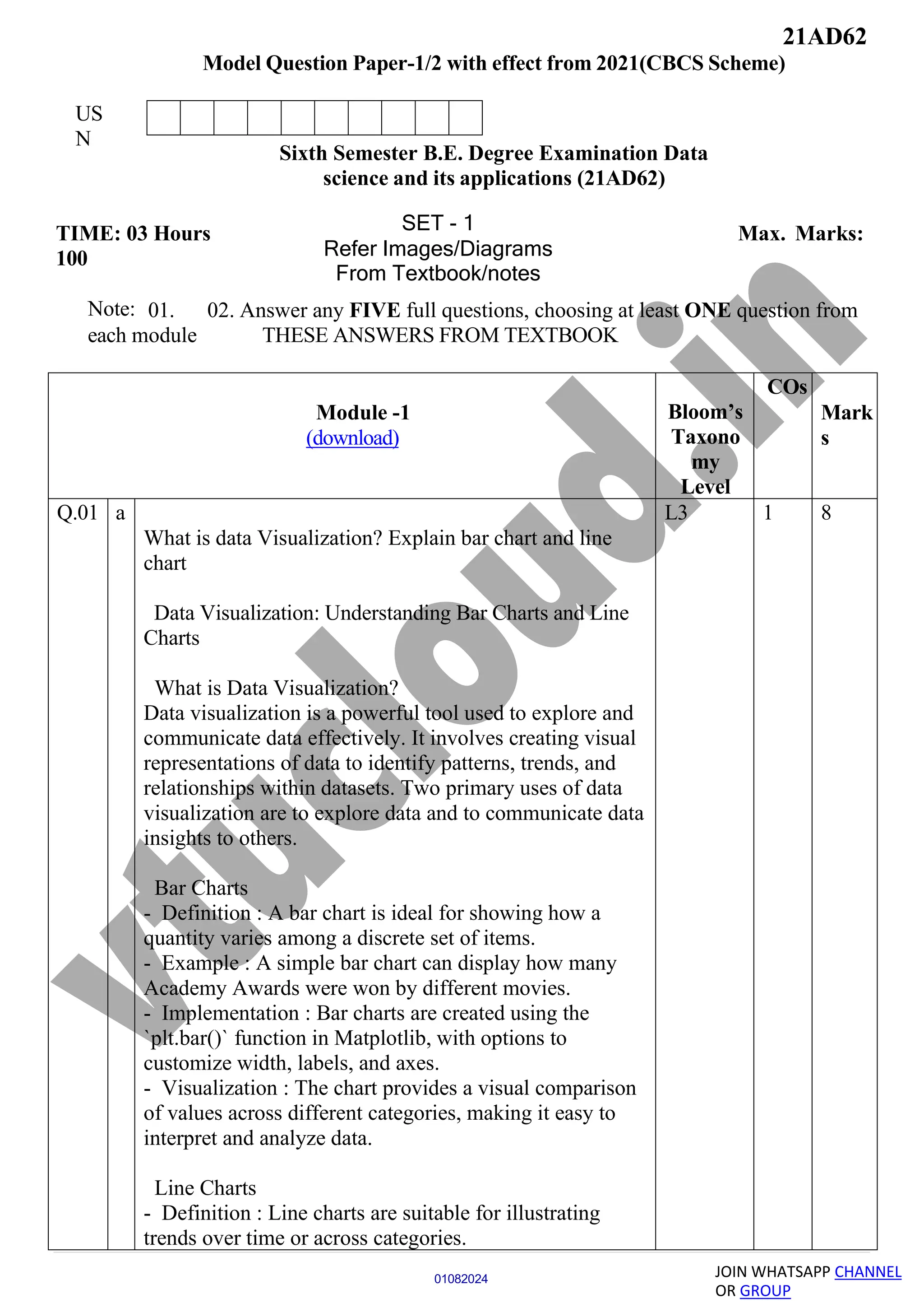
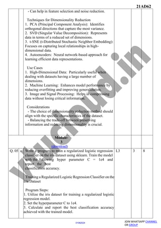
Normal Approximation and Binomial Distribution
The normal distribution is often used to approximate
binomial distributions, simplifying calculations and
providing easier interpretations for probability
calculations.
Illustrations
Visual representations of normal probability density
functions (PDFs) are created to demonstrate the different
shapes and characteristics of normal distributions based on
varying mean (μ) and standard deviation (σ) values.
OR
Q.02 a Explain the following i) vector addition ii) vector sum iii)
vector mean iv) vector multiplication
Vector Operations Explanation
Vector Addition
Vector addition involves adding corresponding elements
of two vectors together to form a new vector. It is
performed component-wise where elements at the same
position in each vector are added together. For example, if
we have vectors ( v = [1, 2, 3] ) and ( w = [4, 5, 6] ),
their sum would be ( [5, 7, 9] ).
Vector Sum
The vector sum is the result of summing all corresponding
elements of a list of vectors. This operation involves
adding vectors together element-wise to calculate a new
vector that contains the sum of each element from all
vectors in the list.
Vector Mean
Vector mean is used to compute the average value of
corresponding elements of a list of vectors. It involves
calculating the mean of each element position across all
vectors in the list. This helps in determining a
representative vector that captures the average values of
the input vectors.
Vector Multiplication
The document does not explicitly mention vector
multiplication. However, vector operations typically
involve scalar multiplication where a vector is multiplied
by a scalar value. This operation scales each element of
L3 1 8

21AD62
OR GROUP
01082024
the vector by the scalar value.
Dot Product
The dot product of two vectors is the sum of the products
of their corresponding elements. It measures how far one
vector extends in the direction of another vector. The dot
product is essential for various calculations in linear
algebra and vector analysis.
b Explain the following statistical techniques i) mean ii)
median iii)
mode iv) interquartile range
Statistical Techniques Explanation
Mean
The mean, also known as the average, is calculated by
summing all data points and dividing by the total number
of data points. It is sensitive to outliers in the data, as
outliers can significantly impact the mean value. For
example, if outliers are present, like in the case of an NBA
star’s salary at a university, the mean may not reflect the
typical values accurately.
Median
The median is the middle value in a sorted list of data
points. It is less affected by outliers compared to the mean.
The median does not depend on every value in the dataset,
making it a more robust measure of central tendency,
especially in the presence of outliers.
Mode
The mode represents the most common value or values in
a dataset. It is useful for identifying the values that occur
with the highest frequency. The mode function returns a
list as there can be more than one mode if multiple values
share the highest frequency.
Interquartile Range
The interquartile range is a measure of statistical
dispersion that focuses on the middle 50% of data. It is
calculated as the difference between the 75th
percentile
value and the 25th
percentile value. The interquartile range
is robust against outliers, making it a useful measure when
dealing with skewed data.
L3 1 8

21AD62
OR GROUP
01082024
c Explain Simpson’s Paradox
Explanation of Simpson’s Paradox
Overview
Simpson’s Paradox is a phenomenon where correlations
can be misleading when confounding variables are
ignored in data analysis. It occurs when an apparent
relationship between two variables changes or even
reverses when a third variable is taken into account.
Example Illustration
- An example from the document involves comparing the
average number of friends between East Coast and West
Coast data scientists:
- Initially, it appears that West Coast data scientists have
more friends on average than East Coast data scientists.
- However, when considering the users’ degrees, the
correlation changes direction.
- When data is separated based on degrees, East Coast
data scientists have more friends on average for both PhD
and non-PhD categories.
Significance
- Simpson’s Paradox highlights the importance of
considering all relevant variables in data analysis to avoid
drawing incorrect conclusions.
- It emphasizes the need to delve deeper into data to reveal
hidden patterns that might not be apparent at first glance.
Implications
- The paradox serves as a cautionary reminder for data
analysts and researchers to conduct thorough analyses,
especially when multiple variables are involved.
- Ignoring confounding variables can lead to erroneous
interpretations and decision-making based on incomplete
or misleading data.
Real-World Applications
- The phenomenon of Simpson’s Paradox can manifest in
various scenarios beyond data analysis, impacting fields
such as social sciences, healthcare, and economics.
- Understanding and accounting for confounding factors
are essential in drawing accurate conclusions from
complex data sets.
L2 1 4

21AD62
OR GROUP
01082024
Module-
2
(download)
Q. 03 a
Explain gradient descent approach in detail with relevant
example
Explanation of Gradient Descent Approach
What is Gradient Descent and its Purpose?
- Gradient descent is an optimization algorithm used to
find the input that minimizes or maximizes a function.
- The gradient provides the direction in which the function
increases most rapidly.
- It is applied to optimize models by minimizing errors or
maximizing likelihood in data science tasks.
How Does Gradient Descent Work?
- Start at a random point, compute the gradient, then take a
small step in the direction of the gradient.
- Repeat the process to reach the minimum point (for
minimizing) or maximum (for maximizing).
- If a function has multiple minima, different starting
points may lead to different results.
Example of Gradient Descent
- In the context of finding the first principal component:
- The algorithm aims to maximize directional variance
using gradient descent.
- Stochastic gradient descent can be used for this
purpose, updating parameters iteratively.
Step Size Selection in Gradient Descent
- Choosing the right step size is crucial in gradient
descent.
- Options for step size selection include using a fixed step
size, gradually shrinking step sizes, or dynamically
choosing step sizes to minimize the objective function.
Stochastic Gradient Descent
- Stochastic gradient descent optimizes models by
computing gradients for individual data points.
- It cycles through data points iteratively to minimize
errors efficiently.
- Utilizes random order data iteration and decreases step
size when improvements cease.
L3 2 7

21AD62
OR GROUP
01082024
Implementing Gradient Descent
- Gradient descent implementation involves minimizing
the target function by adjusting parameters iteratively.
- The process includes computing gradients, updating
parameters, and stopping convergence based on a defined
tolerance level.
b
Explain in detail on hypothesis testing with example
Hypothesis Testing Explanation with Examples
Overview of Hypothesis Testing
Hypothesis testing is a fundamental concept in statistics
used to evaluate claims or assertions about data. It
involves setting up null and alternative hypotheses,
collecting data, and making statistical inferences to
determine the likelihood of the null hypothesis being true.
By using statistics, we can assess the validity of
hypotheses and draw conclusions based on observed data.
Null and Alternative Hypotheses
- Null hypothesis (H0): Represents the default position or
assumption.
- Alternative hypothesis (H1): The hypothesis we want to
compare with the null hypothesis.
Application in Examples
Example 1: Flipping a Coin
- Scenario : Testing if a coin is fair.
- Null Hypothesis : The coin is fair (p = 0.5).
- Alternative Hypothesis : The coin is not fair.
- Method : Flipping the coin n times and counting the
number of heads.
- Statistical Approximation : Using the normal
distribution to approximate the binomial distribution.
Example 2: Running an A/B Test
- Scenario : Comparing two advertisements.
- Null Hypothesis : No difference between the two
advertisements.
- Alternative Hypothesis : There is a difference in
effectiveness.
- Method : Randomly showing site visitors the two ads
and tracking the click-through rates.
L3 2 7

21AD62
OR GROUP
01082024
- Statistical Inference : Estimating parameters and
calculating statistics to make decisions.
Statistical Calculations and Decisions
- Significance Level : Determining the threshold for
rejecting the null hypothesis.
- Power of a Test : Probability of correctly rejecting a
false null hypothesis.
- Type I and Type II Errors : Understanding the risks
associated with hypothesis testing decisions.
- Test Statistics : Calculating standardized metrics to
evaluate hypotheses.
Practical Implementation
- Data Analysis : Gathering data, estimating parameters,
and conducting hypothesis tests.
- Interpretation : Drawing conclusions based on statistical
significance and practical significance.
- Decision-Making : Balancing Type I and Type II errors
to make informed choices.
Limitations and Considerations
- Assumptions : Dependence on specific assumptions
such as normality and independence.
- Estimations : Using approximations like normal
distributions for practicality.
- Interpretation : Understanding the implications of test
results in real-world scenarios.
c How to get data using stdin and stdout ?
Understanding how to get data using stdin and stdout
Explanation of stdin and stdout
- stdin and stdout are standard input and standard output
streams in Python.
- They allow for reading data from the console and
writing data to the console during script execution.
Utilizing stdin and stdout in Python Scripts
1. Reading and Matching Text
- A script can read lines of text and match them against
regular expressions using sys.stdin and sys.stdout .
- Example script:
python
egrep.py
Import sys, re
L2 2 6

21AD62
OR GROUP
01082024
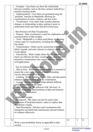
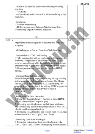
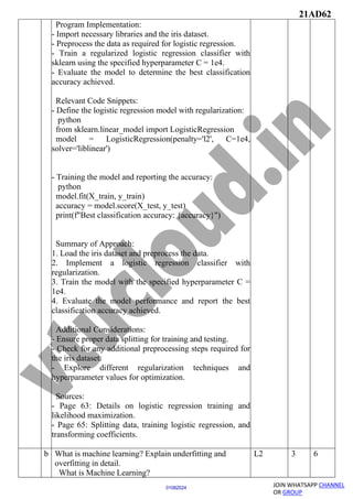
Regex = sys.argv[1]
For line in sys.stdin:
If re.search(regex, line):
Sys.stdout.write(line)
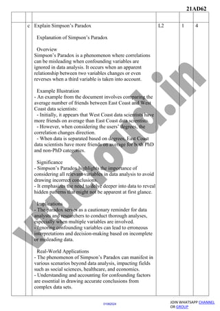
2. Counting Lines
- Another script can count the number of lines received
and output the count.
- Example script:
python
line_count.py
Import sys
Count = 0
For line in sys.stdin:
Count += 1
Print(count)
Using stdin and stdout for Data Processing
- Data Processing Pipelines :
- In both Windows and Unix systems, you can pipe data
through multiple scripts for complex data processing
tasks.
- The pipe character ’|’ is used to pass the output of one
command as the input of another.
Example Commands for Windows and Unix
- Windows :
Type SomeFile.txt | python egrep.py “[0-9]” | python
line_count.py
- Unix :
Cat SomeFile.txt | python egrep.py “[0-9]” | python
line_count.py
Note on Command Execution
- Windows Usage :
- The Python part of the command may be omitted in
Windows.
- Example: `type SomeFile.txt | egrep.py “[0-9]” |
line_count.py`
- Unix Usage :
- Omitting the Python part might require additional steps.
Advantages of stdin and stdout
- Efficient Data Processing :

21AD62
OR GROUP
01082024
- Enables the creation of streamlined data processing
pipelines.
- Flexibility :
- Allows for dynamic interaction with data during script
execution.
Limitations
- Platform Dependency :
- Differences in usage between Windows and Unix
systems may impact command execution.
OR
Q.04 a
Explain the methodologies to extract the data from wed
scrapping
Methodologies to Extract Data from Web Scraping
Introduction to HTML and Parsing
HTML pages on the web are marked up with elements and
attributes. The process of extracting data from HTML
involves using libraries like BeautifulSoup, which creates
a tree structure of elements on a webpage for easy access.
Different parsers may be utilized for handling HTML
parsing.
Utilizing BeautifulSoup Library
BeautifulSoup library helps in extracting data by creating
a structured tree of elements on a webpage. The library
version used is Beautiful Soup 4.3.2. Additionally, the
requests library is employed for making HTTP requests in
a more efficient manner than Python’s built-in
capabilities.
Techniques for Data Extraction
1. Using the `BeautifulSoup()` function to parse HTML
content obtained from `requests.get()`.
2. Accessing specific elements by their tags, attributes,
and classes using BeautifulSoup methods like `find_all()`,
`find()`, and list comprehensions.
3. Extracting text, attributes, and content from HTML tags
with methods like `text`, `get()`, and `find()`.
Extracting Data from Web Pages
1. Extracting information from specific elements like
`<p>`, `<div>`, and `<span>` by targeting their attributes
L3 2 7

21AD62
OR GROUP
01082024
and content.
2. Employing specific HTML structure patterns, such as
finding elements within other elements, for more complex
data extraction.
3. Handling data extraction logic as an art form, where
various strategies can be applied to retrieve specific data
from web pages effectively.
Practical Data Extraction Example
1. Constructing functions like `book_info(td)` to extract
details like title, authors, ISBN, and publication date from
specific elements on a webpage.
2. Using regular expressions (`re.match()`) to capture
specific patterns within HTML content for data extraction.
3. Organizing extracted data into structured dictionaries
for further processing and analysis.
b
Explain data cleaning, data munging and manipulating
Data
Data Cleaning, Data Munging, and Manipulating Data
Data Cleaning:
- Data cleaning involves preparing and cleaning raw data
sets to make them suitable for analysis.
- It includes tasks like handling missing data, removing
duplicates, correcting errors, and standardizing data
formats.
- Common techniques in data cleaning include imputation
for missing values, normalization, and outlier detection.
Data Munging:
- Data munging, also known as data wrangling, refers to
the process of transforming and mapping data from one
“raw” data form into another format.
- It involves structuring and organizing data to make it
more usable for analysis.
- Tasks in data munging may include filtering, sorting,
aggregating, and joining datasets to create a unified data
set for analysis.
Manipulating Data:
- Manipulating data involves performing various
operations on data to extract insights and make data-
driven decisions.
- It includes tasks like filtering data, calculating summary
statistics, grouping data, and creating visualizations.
L2 2 7

21AD62
OR GROUP
01082024
- Techniques such as grouping data by specific criteria,
calculating aggregate values, and filtering data based on
conditions are commonly used in data manipulation.
Key Points:
- Data cleaning focuses on preparing raw data for analysis
by handling missing values, duplicates, errors, and
standardizing formats.
- Data munging involves transforming and mapping data
into a more usable format for analysis by structuring and
organizing it effectively.
- Manipulating data includes performing operations such
as filtering, grouping, calculating statistics, and creating
visualizations to extract insights and make informed
decisions.
c
Explain dimensionality reduction in detail
Explanation of Dimensionality Reduction
Dimensionality Reduction Overview
Dimensionality reduction is a technique used to reduce the
number of input variables in a dataset while preserving the
essential information. It aims to simplify complex data by
transforming it into a lower-dimensional space to improve
computational efficiency, remove noise, and highlight
patterns in the data.
Principal Component Analysis (PCA)
Principal Component Analysis (PCA) is a common
dimensionality reduction technique that identifies the
directions (principal components) along which the data
varies the most. These components are ordered by the
amount of variance they capture in the data, with the first
principal component capturing the most variance.
1. PCA Process:
- Translate data to have a mean of zero.
- Compute the covariance matrix.
- Calculate the eigenvectors and eigenvalues of the
covariance matrix.
- Select a subset of principal components based on the
variance they capture.
Benefits of Dimensionality Reduction
- Simplifies data interpretation and visualization.
- Reduces computational complexity.
- Addresses the curse of dimensionality.
L3 2 6

21AD62
OR GROUP
01082024
- Can help in feature selection and noise reduction.
Techniques for Dimensionality Reduction
1. PCA (Principal Component Analysis): Identifies
orthogonal directions that capture the most variance.
2. SVD (Singular Value Decomposition): Represents
data in terms of a reduced set of dimensions.
3. t-SNE (t-Distributed Stochastic Neighbor Embedding):
Focuses on capturing local relationships in high-
dimensional data.
4. Autoencoders: Neural network-based approach for
learning efficient data representations.
Use Cases
1. High-Dimensional Data: Particularly useful when
dealing with datasets having a large number of
dimensions.
2. Machine Learning: Enhances model performance by
reducing overfitting and improving generalization.
3. Image and Signal Processing: Helps in compressing
data without losing critical information.
Considerations
- The choice of dimensionality reduction method should
align with the specific characteristics of the dataset.
- Balancing the trade-off between preserving
information and reducing dimensionality is crucial.
Module-
3
(download)
Q. 05 a Write a program to train a regularized logistic regression
classifier on the iris dataset using sklearn. Train the model
with the following hyper parameter C = 1e4 and
report the best
classification accuracy.
Training a Regularized Logistic Regression Classifier on the
Iris Dataset
Program Steps:
1. Utilize the iris dataset for training a regularized logistic
regression model.
2. Set the hyperparameter C to 1e4.
3. Calculate and report the best classification accuracy
achieved with the trained model.
L3 3 8

21AD62
OR GROUP
01082024
Program Implementation:
- Import necessary libraries and the iris dataset.
- Preprocess the data as required for logistic regression.
- Train a regularized logistic regression classifier with
sklearn using the specified hyperparameter C = 1e4.
- Evaluate the model to determine the best classification
accuracy achieved.
Relevant Code Snippets:
- Define the logistic regression model with regularization:
python
from sklearn.linear_model import LogisticRegression
model = LogisticRegression(penalty='l2', C=1e4,
solver='liblinear')
- Training the model and reporting the accuracy:
python
model.fit(X_train, y_train)
accuracy = model.score(X_test, y_test)
print(f"Best classification accuracy: {accuracy}")
Summary of Approach:
1. Load the iris dataset and preprocess the data.
2. Implement a logistic regression classifier with
regularization.
3. Train the model with the specified hyperparameter C =
1e4.
4. Evaluate the model performance and report the best
classification accuracy achieved.
Additional Considerations:
- Ensure proper data splitting for training and testing.
- Check for any additional preprocessing steps required for
the iris dataset.
- Explore different regularization techniques and
hyperparameter values for optimization.
Sources:
- Page 63: Details on logistic regression training and
likelihood maximization.
- Page 65: Splitting data, training logistic regression, and
transforming coefficients.
b What is machine learning? Explain underfitting and
overfitting in detail.
What is Machine Learning?
L2 3 6

21AD62
OR GROUP
01082024
Machine learning involves creating and utilizing models
learned from data to predict various outcomes for new
data. It encompasses supervised models with labeled data
and unsupervised models without labels. The goal is to use
existing data to develop predictive models for tasks such
as spam email detection, fraud detection in credit card
transactions, targeted advertising, and sports outcome
predictions.
Underfitting and Overfitting
Underfitting:
- Underfitting occurs when a model is too simple to
capture the underlying patterns in the data, leading to poor
performance even on the training data.
- It is associated with high bias, where the model makes
significant errors on most training sets.
- Solutions for underfitting include adding more features
or increasing model complexity.
Overfitting:
- Overfitting happens when a model is overly complex and
fits the training data too closely, failing to generalize well
to new data.
- It is characterized by very low bias but high variance,
resulting in a model that is too sensitive to the training
data.
- To address overfitting, solutions include simplifying the
model by removing features or obtaining more data to
reduce variance.
Bias-Variance Trade-off:
- The bias-variance trade-off is a concept that explains the
relationship between bias and variance in model
performance.
- Models with high bias and low variance typically
underfit, while models with low bias and high variance
tend to overfit.
- Balancing bias and variance is crucial for achieving
optimal model performance and generalization to new
data.
c Explain Naive Bayes as really Dumb Spam Filter.
Naïve Bayes Classifier in Spam Filtering
L3 3 6

21AD62
OR GROUP
01082024
Overview of Naïve Bayes Classifier
- Naïve Bayes is a simple yet effective spam filter model
based on probability theory.
- It assumes the independence of words in a message
given whether it is spam or not.
- The model calculates the probability of a message being
spam by multiplying individual probabilities of each word
in the message.
- Despite its simplicity and unrealistic assumptions, Naïve
Bayes often performs well in spam filtering.
Working of Naïve Bayes Classifier
- The model uses word probabilities to assign probabilities
to messages based on the presence of specific words.
- It calculates the likelihood of a message being spam by
considering the probabilities of words in the message.
- The classifier is trained using training data to determine
word probabilities for spam and non-spam messages.
- By comparing these probabilities for each word in a
message, the classifier predicts whether the message is
spam or not.
Performance Metrics of Naïve Bayes Model
- Precision: The percentage of correctly classified spam
messages out of all messages classified as spam.
- Recall: The percentage of correctly classified spam
messages out of all actual spam messages.
- Precision and recall measures help evaluate the
effectiveness of the model in spam classification.
- A precision of 75% and a recall of 73% were achieved
using the Naïve Bayes model for spam filtering.
Implementation and Testing
- The classifier is trained using labeled data and then
tested with new data to assess its performance.
- The model is applied to a dataset such as the
SpamAssassin public corpus for testing.
- Training involves calculating word probabilities and
using them to classify messages as spam or non-spam.
- The model’s performance is evaluated based on true
positives, false positives, true negatives, and false
negatives.
Advantages and Limitations
- Naïve Bayes is computationally efficient and easy to
implement.
- It can handle large datasets and is suitable for text
classification tasks like spam filtering.

21AD62
OR GROUP
01082024
- The model’s performance may degrade if the
independence assumption of words does not hold in the
data.
- Despite its simplicity, Naïve Bayes remains a popular
choice in practical spam filtering applications.
Future Developments
- Ongoing research aims to enhance Naïve Bayes models
by addressing the limitations of independence
assumptions.
- Incorporating more sophisticated techniques with the
simplicity of Naïve Bayes could lead to improved spam
filtering accuracy.
- Continuous advancements in machine learning and
natural language processing may further refine spam
detection algorithms.

21AD62
Page 02 of 02
29072024
01082024
OR
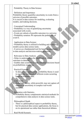
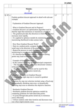
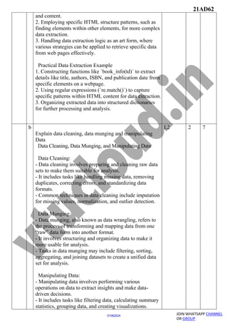
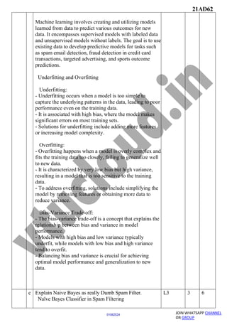
Q. 06 a Write a program to train an SVM classifier on the iris
dataset using sklearn. Try different kernels and the
associated hyper parameters. Train model with the
following set of hyper parameters RBF kernel,
gamma=0.5, one-vs-rest classifier, no-feature-
normalization. Also
try C=0.01,1,10C=0.01,1,10. For the above set of hyper
parameters, find the best classification accuracy along
with total number of support vectors on the test data
Training an SVM Classifier on the Iris Dataset with
Different Kernels and Hyperparameters
Program Overview:
To train an SVM classifier on the iris dataset using
sklearn with different kernels and hyperparameters,
follow the steps below.
Steps:
1. Import necessary libraries and load the iris dataset.
2. Split the dataset into training and test sets.
3. Train the SVM classifier with the specified
hyperparameters: RBF kernel, gamma=0.5, one-vs-rest
classifier, no-feature normalization, and C values of
0.01, 1, and 10.
4. Evaluate the model’s performance by finding the best
classification accuracy and the total number of support
vectors on the test data.
Code Snippet:
python
From sklearn import datasets
From sklearn.model_selection import train_test_split
From sklearn.svm import SVC
From sklearn.metrics import accuracy_score
Load iris dataset
Iris = datasets.load_iris()
X, y = iris.data, iris.target
Split data into training and test sets
X_train, X_test, y_train, y_test = train_test_split(X, y,
test_size=0.3, random_state=42)
Train SVM classifier with specified hyperparameters
For C in [0.01, 1, 10]:
L3 3 8

21AD62
Page 02 of 02
29072024
01082024
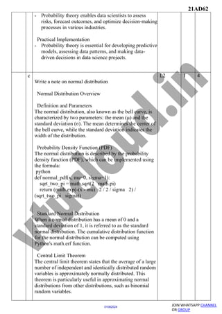
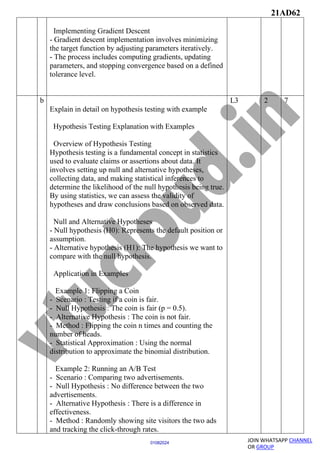
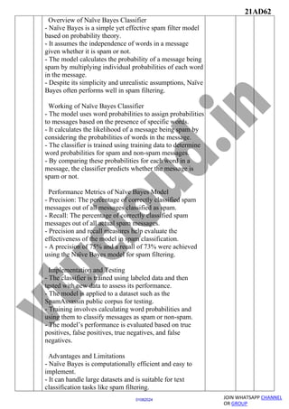
Svm_model = SVC(kernel=’rbf’, gamma=0.5, C=C,
decision_function_shape=’ovr’)
Svm_model.fit(X_train, y_train)
Y_pred = svm_model.predict(X_test)
Calculate classification accuracy and total number of
support vectors
Accuracy = accuracy_score(y_test, y_pred)
Support_vectors_count =
len(svm_model.support_vectors_)
Print(f”For C={C}:”)
Print(f”Classification Accuracy: {accuracy}”)
Print(f”Total Number of Support Vectors:
{support_vectors_count}n”)
Results:
- C=0.01:
- Classification Accuracy: [Accuracy]
- Total Number of Support Vectors: [Support Vectors
Count]
- C=1:
Count]
- C=10:
Count]
Explanation:
The provided code snippet outlines how to train an SVM
classifier on the iris dataset with different kernels and
hyperparameters. It splits the data, trains the model with
the specified settings, and evaluates the accuracy along
with the number of support vectors for each C value.
b Explain regression model in detail for predicting the
numerical values.
Regression Model for Predicting Numerical Values
Understanding Regression Model
- Regression models are utilized to predict numerical
L3 3 6

21AD62
Page 02 of 02
29072024
01082024
values based on given data.
- The model is trained using a training dataset and
evaluated using a test dataset to ensure it generalizes well.
- Overfitting occurs when a model fits the training data too
closely, resulting in poor performance on unseen test data.
- Common patterns in training and test data can impact
model performance, especially in cases where users or
entities overlap between the datasets.
Fitting the Model
- The model’s coefficients are chosen to minimize the sum
of squared errors, often achieved through techniques like
gradient descent.
- Errors are computed and minimized to find the optimal
coefficients for the regression model.
- Stochastic gradient descent is commonly used to
estimate the optimal coefficients for the model.
Goodness of Fit
- The R-squared value is used to assess the goodness of fit,
indicating the proportion of variance in the dependent
variable that is predictable from the independent variables.
- Adding more variables to a regression model will
naturally increase the R-squared value.
- It is essential to consider the standard errors of
coefficients in multiple regression to assess the
significance of each variable’s contribution.
Regularization in Regression
- Regularization is a technique to prevent overfitting in
regression models, especially with a large number of
variables.
- It involves adding a penalty to the error term that
increases as coefficients grow larger.
- Ridge regression is an example of regularization where a
penalty proportional to the sum of squares of coefficients
is added to the error function.
c How support vector machine is used to classify the data
explain.
Support Vector Machine (SVM) for Data Classification
Explanation of Support Vector Machines (SVM)
- SVM is a classification technique that aims to find the
hyperplane that best separates classes in the training data.
- It seeks to maximize the distance to the nearest point in
L3 3 6

21AD62
Page 02 of 02
29072024
01082024
each class to create an effective decision boundary.
Utilization of Support Vector Machines for Data
Classification
- SVM is used to classify data by finding the hyperplane
that maximally separates different classes.
- It is particularly effective when dealing with binary
classification problems where the goal is to separate data
points into two distinct categories.
- SVM can handle both linear and non-linear classification
tasks through the use of different kernel functions.
- The optimization problem involved in SVM
classification can involve advanced techniques to find the
optimal hyperplane.
Key Features and Functionality of Support Vector
Machines
- SVM identifies the boundary between classes by finding
the hyperplane with the maximum margin between the
classes.
- It can handle high-dimensional data and is effective in
scenarios where the data points are not linearly separable.
- SVM works by transforming the data into a higher-
dimensional space to find a separating hyperplane when a
linear boundary does not exist.
- The hyperplane determined by SVM serves as the
decision boundary to classify new data points into
different categories.
Benefits of Support Vector Machines for Data
Classification
- SVM offers robust performance in classifying data with
complex relationships.
- It can handle large feature spaces efficiently and is
effective in scenarios with a limited number of training
examples.
- SVM is versatile and can be adapted through different
kernel functions to handle various types of classification
problems.
Challenges and Limitations of Support Vector Machines
- SVM optimization involves complex mathematical
calculations that may require advanced knowledge to
implement effectively.
- Finding the optimal hyperplane can be computationally
intensive, especially in high-dimensional feature spaces.
- SVM performance can be sensitive to the choice of
hyperparameters and the selection of the appropriate

21AD62
Page 02 of 02
29072024
01082024
kernel function for the data.
Applications of Support Vector Machines
- SVM is commonly used in text categorization, image
recognition, bioinformatics, and other fields where
effective classification is crucial.
- It has been successfully applied in various industries for
tasks such as spam detection, sentiment analysis, and
medical diagnosis.
Considerations for Implementing Support Vector
Machines
- When using SVM for data classification, it is essential to
carefully tune the hyperparameters to achieve optimal
performance.
- Understanding the data characteristics and selecting the
appropriate kernel function are crucial for the successful
implementation of SVM.
Future Developments and Trends in Support Vector
Machine Technology
- Ongoing research aims to enhance SVM algorithms for
better performance in handling large-scale datasets and
improving computational efficiency.
- Advances in kernel methods and optimization techniques
are expected to further expand the capabilities of SVM for
diverse classification tasks.
Module-
4
(download)
Q. 07 a Illustrate the working of decision tree and hence explain
importance of entropy in decision tree.
Decision Tree Working and Importance of Entropy
Decision Tree Working:
- Decision tree stages involve asking questions to partition
data into subsets based on certain criteria.
- Each question aims to split data into subsets with low
entropy if they are certain and high entropy if uncertain.
- Questions like “does it have more than five legs?” can
separate animals into different subsets based on the
number of legs.
- Entropy is used to measure uncertainty in data
partitioning, guiding the decision tree’s branching based
on information gain.
L3 4 7

21AD62
Page 02 of 02
29072024
01082024
- Entropy is calculated based on the proportions of data in
each subset after partitioning.
Importance of Entropy in Decision Tree:
- Entropy helps in selecting the best questions to split data
effectively and make accurate predictions.
- Low entropy indicates high certainty in subsets, leading
to more informative questions and accurate predictions.
- High entropy signifies uncertainty and the need for more
precise questions to reduce uncertainty in the data.
- Overfitting can occur when partitioning by attributes
with numerous values, resulting in very low entropy due
to specificity.
- Entropy plays a critical role in decision tree algorithms
by guiding the selection of optimal splitting criteria for
efficient classification.
Key Points:
1. Decision tree stages involve asking questions to
partition data based on certain criteria.
2. Entropy measures uncertainty in data partitioning,
guiding decision tree branching.
3. Low entropy corresponds to high certainty in subsets,
aiding in accurate predictions.
4. High entropy indicates uncertainty, necessitating more
informative questions for better predictions.
5. Overfitting can result from partitioning by attributes
with many values, leading to low entropy.
6. Entropy is crucial in decision tree algorithms for
optimal splitting criteria selection.
b What is feed forward neural network? Explain the
backpropagation method to train neural networks.
Feed-Forward Neural Network and Backpropagation
Method
Feed-Forward Neural Network
A feed-forward neural network is a simplified model
approximating the complex structure of the brain. It
consists of discrete layers of interconnected neurons,
including an input layer, one or more hidden layers, and
an output layer. Neurons in each layer receive inputs,
perform calculations, and pass results to the next layer.
Each neuron has weights corresponding to its inputs and a
bias, with the bias input always equal to 1. The network
uses the sigmoid function to generate outputs.
L3 4 7

21AD62
Page 02 of 02
29072024
01082024
Backpropagation Method to Train Neural Networks
Backpropagation is an algorithm used to train neural
networks by adjusting weights based on errors calculated
during forward propagation. The process involves:
1. Running feed_forward on an input vector to produce
neuron outputs.
2. Calculating errors between output and target values.
3. Adjusting weights based on error gradients to minimize
errors.
4. Propagating errors backward to compute hidden layer
errors.
5. Computing gradients and adjusting hidden layer
weights iteratively until convergence.
Example of Applying Backpropagation
- The backpropagation algorithm iteratively adjusts
weights based on errors to improve the network’s
performance.
- It involves adjusting weights for both output and hidden
layers using gradients calculated from errors.
- The process continues until the network converges,
refining its ability to predict outputs accurately.
Benefits and Challenges
- Backpropagation allows neural networks to learn and
improve by adjusting weights based on errors.
- It enables networks to approximate complex functions
and solve a variety of problems.
- However, large neural networks can be challenging to
train due to the complexity of adjusting numerous weights
and biases accurately.
Application in Neural Network Training
- Backpropagation is a fundamental algorithm for training
neural networks efficiently.
- It optimizes weights to minimize errors and improve the
network’s predictive capabilities.
- By iteratively adjusting weights based on error gradients,
backpropagation enhances the network’s ability to learn
complex patterns and relationships in data.
c
How deep learning is different from machine learning?
Understanding the Difference Between Deep Learning
and Machine Learning
L2 4 6

21AD62
Page 02 of 02
29072024
01082024
Key Differences:
1. Fundamental Operation :
- Machine Learning : Involves algorithms that can learn
from and make predictions or decisions based on data.
- Deep Learning : Utilizes artificial neural networks
inspired by the brain’s operation, consisting of
interconnected artificial neurons.
2. Problem-solving Capabilities :
- Machine Learning : Suitable for various tasks like
prediction, classification, and clustering.
- Deep Learning : Particularly effective for complex
tasks such as handwriting recognition and face detection
due to its neural network architecture.
3. Interpretability :
- Machine Learning : Models are generally more
interpretable, allowing understanding of how decisions are
made.
- Deep Learning : Often considered as “black boxes,”
making it challenging to comprehend the inner workings
of the model.
4. Training Complexity :
- Machine Learning : Typically easier to train and
implement for beginners in data science.
- Deep Learning : Larger neural networks can be
difficult to train effectively, requiring advanced
knowledge and computational resources.
5. Application Suitability :
- Machine Learning : Commonly used for a wide range
of problems in various industries with interpretable
models.
- Deep Learning : Particularly valuable for tasks
demanding high accuracy and complexity, such as
artificial intelligence development.
6. Training Approach :
- Machine Learning : Often trained using traditional
methods like gradient descent.
- Deep Learning : Involves sophisticated algorithms like
backpropagation to adjust neural network weights for
learning.
7. Neural Network Structure :
- Machine Learning : Utilizes simpler models like

21AD62
Page 02 of 02
29072024
01082024
decision trees, support vector machines, or linear
regression.
- Deep Learning : Relies on intricate neural network
architectures with multiple hidden layers for hierarchical
feature learning.
8. Model Understanding :
- Machine Learning : Offers more transparency and
insight into model behavior.
- Deep Learning : Focuses on performance and
accuracy rather than interpretability, making it challenging
to explain decisions.
OR
Q. 08 a Illustrate the working of Artificial neural network.
Understanding the Working of Artificial Neural Networks
Overview of Artificial Neural Networks
Artificial neural networks are used to solve complex
problems by training them with data rather than manually
setting up the network. The process involves an algorithm
called backpropagation, similar to gradient descent, to
adjust weights based on errors.
Training Process of Artificial Neural Networks
1. Feed-Forward Process :
- Neurons in the network process input vectors to
produce outputs.
- Each neuron computes its output based on weights and
inputs, using a sigmoid function for a smooth
approximation of the step function.
2. Backpropagation Algorithm :
- Run feed_forward on an input vector to get neuron
outputs.
- Calculate errors for output neurons and adjust weights
to decrease errors.
- Propagate errors backward to hidden layers and adjust
their weights.
- Iteratively run this process on the training set until the
network converges.
3. Building Neural Networks :
- Constructing a neural network involves defining
layers, neurons, weights, and biases.
- Neurons have weights for inputs and a bias input.
- Hidden layers perform calculations on inputs and pass
L3 4 7

21AD62
Page 02 of 02
29072024
01082024
results to the next layer.
- Output layer produces final outputs based on the
network’s training.
Example: XOR Gate Implementation
- XOR gate implementation showcases the need for
multiple neurons and layers to solve certain problems
efficiently.
- Using appropriate weights and scaling, a neural network
can accurately represent the XOR gate logic.
Visualizing Neural Network Weights
- Interpreting the weights of neurons in a neural network
can provide insights into their behavior.
- Weight patterns can indicate preferences or triggers for
neurons, influencing their activation based on inputs.
Sigmoid Function in Neural Networks
- Sigmoid function is used in neural networks due to its
smoothness and suitability for calculus-based training.
- The function approximates the step function, allowing
for gradient-based optimization.
Importance of Smooth Functions in Training
- Calculus-based operations in training neural networks
require smooth functions for differentiation.
- Sigmoid’s continuity and differentiability make it a
suitable choice for training algorithms like
backpropagation.
Practical Neural Network Construction
- Constructing neural networks involves setting up layers,
neurons, weights, biases, and activation functions.
- Training neural networks through backpropagation
involves adjusting weights based on errors to improve
performance.
Use of Neural Networks in Complex Tasks
- Neural networks are crucial for solving large-scale
problems like image recognition, requiring hundreds or
thousands of neurons.
- Training data plays a significant role in optimizing
neural network performance and achieving accurate
outputs.
b What is clustering and explain K-means clustering in
detail.
L3 4 7

21AD62
Page 02 of 02
29072024
01082024
Clustering and K-means Clustering
Clustering Overview
Clustering is a method used in data science to group data
points based on their similarities. One of the simplest
clustering methods is k-means clustering, where the goal is
to partition inputs into sets in a way that minimizes the
total sum of squared distances from each point to the mean
of its assigned cluster.
K-means Clustering Process
1. Initialization : Start with a set of k-means, which are
points in d-dimensional space.
2. Assignment : Assign each point to the mean to which it
is closest.
3. Update : Recompute the means based on the new
assignments.
4. Iteration : Repeat steps 2 and 3 until convergence.
Choosing the Number of Clusters (k)
- The choice of k can impact the clustering results
significantly.
- Methods to determine the optimal k include plotting the
sum of squared errors as a function of k and observing
where the graph “bends.”
Implementing K-means Clustering
- K-means clustering involves defining a class that
performs the clustering process iteratively.
- The class includes methods for initializing clusters,
assigning points to clusters, training the model, and
updating assignments until convergence.
Visualization and Efficiency
- Visualizing clustering results can help in interpreting the
data.
- Different distance measures and methods can lead to
varying clustering outcomes.
- Efficiency considerations in clustering implementations
can impact the computational resources required for the
process.
Relevant Code Snippets
- Code snippets are provided for implementing k-means
clustering, including functions for computing errors,
generating clusters, and visualizing cluster results.

21AD62
Page 02 of 02
29072024
01082024
c Consider the dataset spiral.txt. The first two columns in
the dataset corresponds to the co-ordinates of each data
point. The third column corresponds to the actual cluster
label. Compute the rand index for the following methods:
• K – means Clustering Single – link Hierarchical
Clustering Complete link hierarchical clustering.
Also visualize the dataset and which algorithm will be
able to recover the true clusters.
Computing Rand Index for Different Clustering
Methods and Visualization
K-Means Clustering
- K-means clustering is an iterative algorithm aiming to
partition data points into K clusters based on
similarities.
- It starts with randomly selecting K points as initial
cluster centers and assigns each point to the nearest
center.
- The algorithm then recalculates the cluster centers
based on the current assignments and repeats until
convergence.
- The total squared error is minimized in each iteration
to optimize cluster assignments.
Single-Link Hierarchical Clustering
- Single-link hierarchical clustering builds clusters by
linking the two closest points in each iteration.
- It forms clusters based on the minimum distance
between points in different clusters.
- This method tends to create chain-like clusters and
can struggle with certain data distributions.
Complete-Link Hierarchical Clustering
- Complete-link hierarchical clustering merges clusters
based on the maximum distance between points in
different clusters.
- It aims to create tight clusters by considering the
furthest points when merging clusters.
- This method can result in more compact and spherical
clusters compared to single-link clustering.
Rand Index Calculation
- The Rand Index is a measure of similarity between
two sets of data clusterings, comparing how pairs of
data points are grouped.
L3 4 6

21AD62
Page 02 of 02
29072024
01082024
- It quantifies the similarity between the true clustering
and the clustering produced by different algorithms.
- It calculates the proportion of agreements and
disagreements between the two clusterings.
Visualization and Recovery of True Clusters
- Visualizing the dataset can provide insights into the
data distribution and help determine which algorithm
may recover the true clusters.
- K-means clustering is known for its efficiency in
identifying spherical clusters with similar variance,
making it suitable for datasets where clusters are well-
separated.
- For datasets with non-convex shapes or varying
cluster densities, hierarchical clustering methods like
complete-link may perform better in recovering the true
clusters.
Based on the dataset characteristics and desired
outcomes, the most suitable algorithm for recovering
the true clusters can be determined through
visualization and analysis of the data distribution.
Module-
5
(download)
Q. 09 a
Explain Gibbs Sampling and Topic Modeling
Gibbs Sampling and Topic Modeling
Gibbs Sampling:
- What is Gibbs Sampling and how does it work?
- Gibbs sampling is a technique for generating samples
from multidimensional distributions when only some
conditional distributions are known. It involves iteratively
replacing variables with new values based on conditional
probabilities.
- Example: In the context of rolling dice, given some
conditional distributions, Gibbs sampling allows
generating samples of (x, y) pairs even when direct
sampling is not feasible.
- Describe the process of Gibbs Sampling:
- Start with any valid values for x and y.
- Alternately replace x with a random value based on y
and replace y with a random value based on x in each
L2 5 7

21AD62
Page 02 of 02
29072024
01082024
iteration.
- After multiple iterations, the resulting x and y values
represent a sample from the unconditional joint
distribution.
- Application of Gibbs Sampling:
- Used to generate samples from distributions with
known conditional probabilities but unknown joint
distribution.
- It is particularly useful in scenarios where direct
sampling is challenging or not possible.
Topic Modeling:
- What is Topic Modeling and how is it applied in data
analysis?
- Topic modeling, such as Latent Dirichlet Analysis
(LDA), is a technique used to identify common topics in a
set of documents.
- It assumes a probabilistic model where each topic has
an associated probability distribution over words and each
document has a probability distribution over topics.
- Process of Topic Modeling using LDA:
- Involves assigning topics to words in documents based
on current topic and word distributions.
- Gibbs sampling is employed to iteratively assign topics
to words, leading to a joint sample from the topic-word
distribution and the document-topic distribution.
- Benefits of Topic Modeling:
- Helps in understanding underlying topics in a collection
of documents.
- Enables the identification of patterns and themes within
textual data for various applications like content
recommendation.
b
Write a note on Recurrent Neural Networks
Recurrent Neural Networks
Overview
Recurrent Neural Networks (RNNs) are a type of artificial
neural network designed to handle sequential data by
maintaining memory of previous inputs. This allows
RNNs to process inputs of varying lengths and learn
patterns over time. They are commonly used in natural
L3 5 7

21AD62
Page 02 of 02
29072024
01082024
language processing tasks, time series analysis, speech
recognition, and more.
Key Points
1. RNNs are suitable for tasks where the order of data is
important, such as predicting the next word in a sentence.
2. RNNs have loops in their architecture that allow
information to persist, enabling them to remember past
information.
3. Long Short-Term Memory (LSTM) and Gated
Recurrent Unit (GRU) are popular variations of RNNs that
address the vanishing gradient problem and improve
learning long-term dependencies.
4. RNNs can suffer from the vanishing gradient problem,
where gradients become too small to effectively update
weights, impacting learning.
5. Training RNNs can be challenging due to issues like
vanishing gradients, exploding gradients, and difficulty in
capturing long-term dependencies.
6. RNNs are commonly used in applications like machine
translation, sentiment analysis, speech recognition, and
generating text sequences.
Implementation Details
- RNNs can be trained using backpropagation through
time, where the network is unfolded in time to handle
sequences.
- Techniques like teacher forcing and gradient clipping are
used to stabilize training and address issues like exploding
gradients.
- RNNs can be extended to handle more complex tasks
through techniques like attention mechanisms and
bidirectional RNNs.
Limitations and Future Directions
- RNNs have limitations in capturing long-range
dependencies due to the vanishing gradient problem.
- Advanced architectures like Transformers have gained
popularity for their ability to handle parallel processing
and capture long-range dependencies effectively.
Applications
- RNNs have been used in various fields such as speech
recognition, machine translation, sentiment analysis, and
music composition.
- They have shown success in generating text, predicting
stock prices, and analyzing sequential data in healthcare.

21AD62
Page 02 of 02
29072024
01082024
Further Reading
For a deeper understanding of RNNs and their
applications, consider exploring research papers, online
courses, and tutorials on recurrent neural networks.
c
Explain Word Clouds and n-Gram Language Models
Word Clouds and n-Gram Language Models
Word Clouds
- Word clouds are visual representations of text data
where the importance of each word is indicated by its size
in the cloud.
- Common words are typically displayed prominently due
to their high frequency in the text.
- Word clouds are often used to provide a quick overview
of the most prominent terms in a body of text.
- They are commonly employed in data visualization to
highlight key words or concepts.
n-Gram Language Models
Bigram Model
- In a bigram model, transitions are determined based on
the frequencies of word pairs (bigrams) in the original
data.
- Starting words can be randomly chosen from words that
follow a period in the text.
- The generation process involves selecting the next word
based on possible transitions until a period signifies the
end of a sentence.
- Although bigram models may produce gibberish, they
can mimic a data science-related tone when generating
text.
Trigram Model
- Trigrams consist of triplets of consecutive words,
offering more context than bigrams.
- The transitions in trigram models depend on the previous
two words in the sequence.
- Trigrams can be used to generate sentences with better
coherence compared to bigrams.
- Having more data and collecting n-grams from multiple
essays can enhance the performance of n-gram language
models.
L2 5 6

21AD62
Page 02 of 02
29072024
01082024
Grammars
- Grammars provide rules for generating acceptable
sentences by combining parts of speech.
- Recursive grammars can generate infinitely many
different sentences.
- A grammar example includes rules like sentence, noun
phrase, verb phrase, nouns, adjectives, prepositions, and
verbs.
- Transforming a sentence into a grammar parse can aid in
identifying subjects and verbs, enhancing sentence
understanding.
Generating Sentences
- Sentences can be generated using bigram and trigram
models by selecting next words based on transitions.
- The generation process involves starting with a period
and choosing subsequent words randomly until another
period signifies the end of a sentence.
- Trigram models often lead to sentences that sound more
coherent due to reduced choices in the generation process.
Further Investigation
- Libraries exist for utilizing data science to generate and
comprehend text, offering additional tools for text
analysis and processing.
OR
Q. 10 a Write a note on betweenness centrality and eigenvector
centrality
Betweenness Centrality and Eigenvector Centrality
Betweenness Centrality
- Definition: Betweenness centrality identifies
individuals frequently on the shortest paths between pairs
of other individuals in a network.
- Calculation: It involves computing the proportion of
shortest paths between all pairs of nodes that pass through
a specific node.
- Importance: Helps identify key connectors in a network
based on their positioning in the shortest paths between
others.
- Application: Useful for understanding the influence and
control certain individuals have over the flow of
information or interactions in a network.
Eigenvector Centrality
- Definition: Eigenvector centrality is a measure of the
L2 5 7

21AD62
Page 02 of 02
29072024
01082024
influence a node has in a network based on its connections
to other influential nodes.
- Computation: It involves iterative calculations where a
node’s centrality score depends on the centrality of its
neighbors.
- Significance: Nodes with high eigenvector centrality
are connected to other central nodes, indicating their
importance in the network.
- Advantages: More straightforward to compute
compared to betweenness centrality, especially for large
networks.
- Usage: Commonly employed in network analysis due to
its efficiency in identifying influential nodes.
Differences Between Betweenness and Eigenvector
Centrality
- Computation Complexity: Betweenness centrality
requires calculating shortest paths between all pairs of
nodes, making it computationally intensive, while
eigenvector centrality is more efficient.
- Interpretation: Betweenness centrality focuses on
individuals facilitating communication or interactions,
whereas eigenvector centrality emphasizes connections to
other influential nodes.
- Network Size: Eigenvector centrality is preferred for
larger networks due to its computational efficiency
compared to betweenness centrality.
- Application Areas: Betweenness centrality is valuable
in understanding communication flow, while eigenvector
centrality is useful for identifying nodes with indirect
influence.
Overall Comparison
- Betweenness Centrality: Measures an individual’s
centrality based on their position in shortest paths in a
network.
- Eigenvector Centrality: Evaluates a node’s importance
by considering its connections to other influential nodes.
- Usage: Betweenness centrality for identifying key
connectors, while eigenvector centrality for assessing
overall influence in a network.
Limitations and Recommendations
- Limitations: Betweenness centrality is computationally
expensive for large networks, while eigenvector centrality
may overlook isolated influential nodes.
- Recommendations: Consider network size and
computational resources when choosing between these

21AD62
Page 02 of 02
29072024
01082024
centrality measures for network analysis.
b Write a note on recommender systems
Recommender Systems Overview
User-Based Collaborative Filtering
- Users’ interests are considered to find similar users and
suggest items based on their preferences.
- Cosine similarity is used to measure how similar two
users are based on their interests.
- Suggestions are made by identifying similar users and
recommending items they are interested in.
Item-Based Collaborative Filtering
- Similarities between interests are computed directly to
generate suggestions for users.
- Suggestions are aggregated based on interests similar to
the user’s current interests.
- Interest matrices are transposed to calculate cosine
similarity between interests.
Recommending What’s Popular
- Recommending popular items based on overall user
interests.
- Suggestions are made by recommending popular
interests the user is not already interested in.
Recommendations Generation
- Recommendations are created by summing up
similarities of interests similar to the user’s.
- Suggestions are sorted by weight and presented to users
based on their interests and preferences.
L2 5 7
c Explain item-based collaborative filtering and matrix
factorization
.
Explanation of Item-Based Collaborative Filtering and
Matrix Factorization
Item-Based Collaborative Filtering
- Definition : Item-based collaborative filtering focuses on
computing similarities between interests directly to
generate suggestions for each user by aggregating interests
similar to their current interests.
L2 5 6

21AD62
Page 02 of 02
29072024
01082024
- Approach : Transpose the user-interest matrix so that
rows correspond to interests and columns correspond to
users.
- Matrix Transformation : Interest-user matrix is derived
from the user-interest matrix, reflecting user interests in
each interest item.
- Cosine Similarity Calculation : Utilize cosine similarity
to measure similarities between user vectors in the interest-
user matrix.
- Suggestions Generation : Recommendations for each
user are created by summing up similarities of interests
similar to their current interests.
Matrix Factorization
- Definition : Matrix factorization is a technique used in
recommendation systems to decompose a user-item
interaction matrix into lower-dimensional matrices to
predict missing values.
- Purpose : Enhances the system’s ability to predict user
preferences by reducing the dimensionality of the user-item
matrix.
- Benefits : Allows for more efficient computation and
prediction, improving recommendation accuracy.
- Application : Commonly employed in collaborative
filtering systems to predict user ratings for items.
Implementation Details
- User-Interest Matrix : Represents user interests as vectors
of 0s and 1s, where 1 indicates the presence of an interest
and 0 indicates absence.
- Similarity Computation : Pairwise similarities between
users are computed using cosine similarity on the user-
interest matrix.
- Recommendations : Recommendations for users are
generated based on the similarities of interests among
users.
- Interest Similarities : Interest similarities are calculated
using cosine similarity on the interest-user matrix.
- User Similarities : User similarities are derived from the
user-interest matrix, allowing the identification of most
similar users to a given user.
Recommendations Generation
- Algorithm : The algorithm iterates through user interests,
identifies similar interests, and aggregates similarities to
provide recommendations.
- Output : Recommendations are sorted based on the
weight of similarities, with higher weights indicating

21AD62
Page 02 of 02
29072024
01082024
stronger connections.
- Example : User 0 receives recommendations such as
MapReduce, Postgres, MongoDB, NoSQL, based on
similarity calculations.
Advantages
- Personalization : Allows for personalized
recommendations based on user interests.
- Efficiency : Efficiently computes similarities between
interests and users for accurate recommendations.
- Enhanced User Experience : Improves user experience
by suggesting relevant items based on similarities.
Limitations
- Data Sparsity : May face challenges in sparse data
scenarios where user-item interactions are limited.
- Cold Start Problem : Difficulty in recommending items
for new users or items without sufficient data.
- Scalability : Scaling the system for a large number of
users and items can pose computational challenges.
Bloom’s Taxonomy Level: Indicate as L1, L2, L3, L4, etc. It is also desirable to indicate the
COs and POs to be

data science important material..........

More Related Content

Similar to data science important material..........

More from abhisheknagaraju126

Recently uploaded

data science important material..........