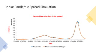
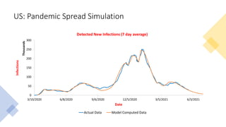
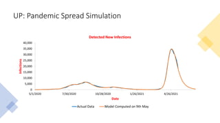
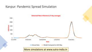
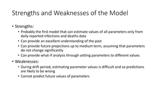
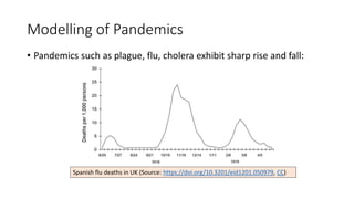
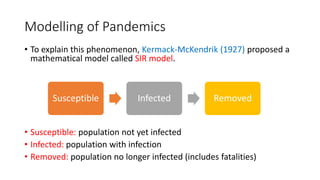
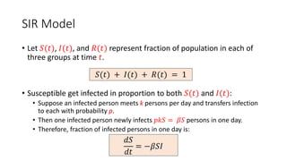
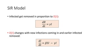
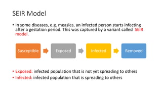
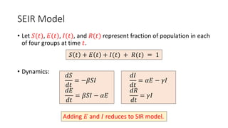
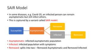
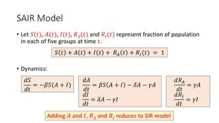
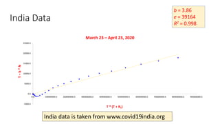
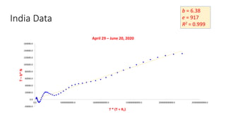
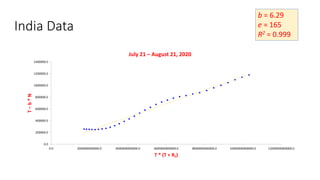
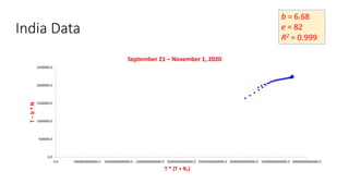
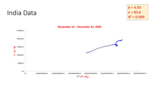
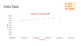
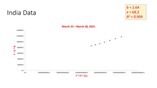
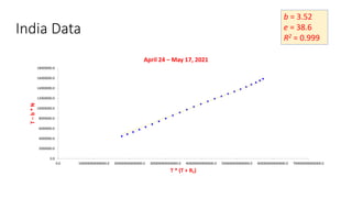
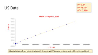
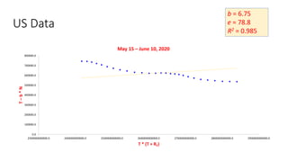
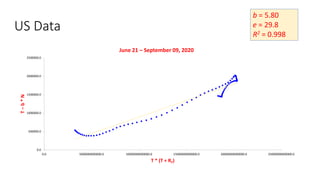
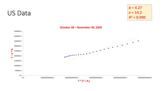
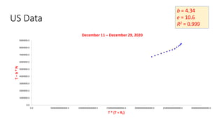
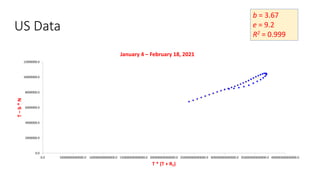
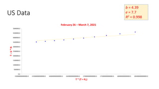
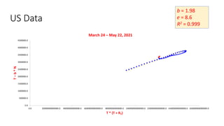
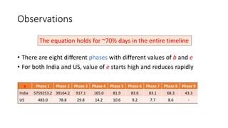
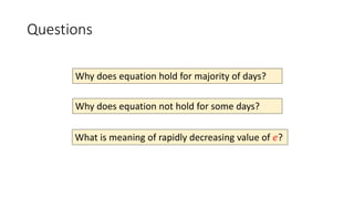
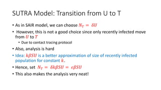
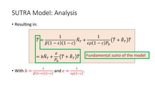
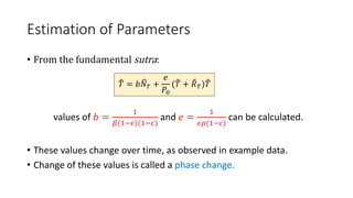
The COVID SUTRA
Manindra Agrawal
IIT Kanpur
Modelling of Pandemics
• Pandemics such as plague, flu, cholera exhibit sharp rise and fall:
Spanish flu deaths in UK (Source: https://doi.org/10.3201/eid1201.050979, CC)
Modelling of Pandemics
• To explain this phenomenon, Kermack-McKendrik (1927) proposed a
mathematical model called SIR model.
• Susceptible: population not yet infected
• Infected: population with infection
• Removed: population no longer infected (includes fatalities)
Susceptible Infected Removed
SIR Model
• Let 𝑆(𝑡), 𝐼(𝑡), and 𝑅(𝑡) represent fraction of population in each of
three groups at time 𝑡.
• Susceptible get infected in proportion to both 𝑆(𝑡) and 𝐼(𝑡):
• Suppose an infected person meets k persons per day and transfers infection
to each with probability p.
• Then one infected person newly infects 𝑝𝑘𝑆 = 𝛽𝑆 persons in one day.
• Therefore, fraction of infected persons in one day is:
𝑆(𝑡) + 𝐼(𝑡) + 𝑅(𝑡) = 1
𝑑𝑆
𝑑𝑡
= −𝛽𝑆𝐼
SIR Model
• Infected get removed in proportion to 𝐼(𝑡):
• 𝐼(𝑡) changes with new infections coming in and earlier infected
removed:
𝑑𝐼
𝑑𝑡
= 𝛽𝑆𝐼 − 𝛾𝐼
𝑑𝑅
𝑑𝑡
= 𝛾𝐼
SIR Model
• Fatalities 𝐷(𝑡) are a subset of 𝑅(𝑡) and change in 𝐷(𝑡) is also
proportional to 𝐼(𝑡):
• Constants 𝛽, 𝛾, and 𝜂 determine the trajectory of the pandemic.
𝑑𝐷
𝑑𝑡
= 𝜂𝐼
Traditionally estimated by studying virus properties,
population dynamics, and healthcare infrastructure.
A Property of SIR Model
• Let 𝑁(𝑡) denote fraction of new infections at time t.
• Then:
• Alternately:
𝑁 = 𝛽𝑆𝐼 = 𝛽 1 − 𝐼 − 𝑅 𝐼 = 𝛽𝐼 − 𝛽 𝐼 + 𝑅 𝐼
𝐼 =
1
𝛽
𝑁 + 𝐼 + 𝑅 𝐼
A Property of SIR Model
• Let 𝑁 𝑡 = 𝑃0𝑁 𝑡 , 𝐼 𝑡 = 𝑃0𝐼 𝑡 , 𝑅 𝑡 = 𝑃0𝑅 𝑡 denote respective
actual numbers at time t.
• Then:
𝐼 =
1
𝛽
𝑁 +
1
𝑃0
𝐼 + 𝑅 𝐼
A Property of SIR Model
• This demonstrates a linear relationship between 𝐼, 𝑁, and 𝐼 + 𝑅 𝐼.
• If above three quantities can be measured, then parameter 𝛽 can be
estimated.
The problem is that reported values of infections may differ greatly
from actual values.
That is why epidemiologists need to use other methods to estimate
parameter values.
SEIR Model
• In some diseases, e.g. measles, an infected person starts infecting
after a gestation period. This was captured by a variant called SEIR
model.
• Exposed: infected population that is not yet spreading to others
• Infected: infected population that is spreading to others
Susceptible Exposed Infected Removed
SEIR Model
• Let 𝑆(𝑡), 𝐸(𝑡), 𝐼(𝑡), and 𝑅(𝑡) represent fraction of population in each
of four groups at time 𝑡.
• Dynamics:
𝑆 𝑡 + 𝐸 𝑡 + 𝐼(𝑡) + 𝑅(𝑡) = 1
𝑑𝑆
𝑑𝑡
= −𝛽𝑆𝐼
𝑑𝐸
𝑑𝑡
= 𝛽𝑆𝐼 − 𝛼𝐸
𝑑𝐼
𝑑𝑡
= 𝛼𝐸 − 𝛾𝐼
𝑑𝑅
𝑑𝑡
= 𝛾𝐼
Adding 𝐸 and 𝐼 reduces to SIR model.
SAIR Model
• In some diseases, e.g. Covid-19, an infected person can remain
asymptomatic but still infect others.
• This is captured by a variant called SAIR model.
• Asymptomatic: infected asymptomatic population
• Infected: infected population with symptoms
• Removed: splits into two – Removed Asymptomatic and Removed Infected
Susceptible Asymptomatic
Removed
Infected Removed
SAIR Model
• Let 𝑆(𝑡), 𝐴(𝑡), 𝐼(𝑡), 𝑅𝐴(𝑡) and 𝑅𝐼(𝑡) represent fraction of population
in each of five groups at time 𝑡.
• Dynamics:
𝑆 𝑡 + 𝐴 𝑡 + 𝐼 𝑡 + 𝑅𝐴 𝑡 + 𝑅𝐼(𝑡) = 1
𝑑𝑆
𝑑𝑡
= −𝛽𝑆(𝐴 + 𝐼)
𝑑𝐴
𝑑𝑡
= 𝛽𝑆 𝐴 + 𝐼 − 𝛿𝐴 − 𝛾𝐴
𝑑𝐼
𝑑𝑡
= 𝛿𝐴 − 𝛾𝐼
𝑑𝑅𝐴
𝑑𝑡
= 𝛾𝐴
𝑑𝑅𝐼
𝑑𝑡
= 𝛾𝐼
Adding 𝐴 and 𝐼, 𝑅𝐴 and 𝑅𝐼 reduces to SIR model
COVID-19 Pandemic
• Different than earlier pandemics:
• Most of these asymptomatic cases are not detected, and continue
passing infection to others.
• Nearly all cases with severe symptoms get detected.
Has a large number of asymptomatic cases
Without detecting, how does one estimate asymptomatic cases?
Modelling Spread of Pandemic
• Due to this, estimating becomes more difficult since even
denominator is not known.
• No model has studied this so far.
The spread of pandemic has been controlled in most countries
How does one estimate spread of the pandemic at different time?
Modelling Spread of Pandemic
• Let 𝑃(𝑡) denote the population of region within reach of the
pandemic at time 𝑡.
• Define 𝜌 = 𝑃/𝑃0, a new parameter that increases over time from 0 to
1, where 𝑃0 is the total population of the region.
• Parameter 𝜌 is called reach of the pandemic.
COVID-19 Pandemic
• On the positive side, extensive data is available for the first time
about pandemic progression in different regions.
• Under-reporting and testing limitations take reported data even
further away from actual numbers.
Can one use reported data to estimate parameter values?
A Question
• Let
• 𝑁𝑇 𝑡 denote fraction of daily reported infections,
• 𝑇(𝑡) fraction of reported active infections, and
• 𝑅𝑇(𝑡) fraction of cumulative removed among reported infections at time t.
• Data available is 𝑇 𝑡 = 𝜌𝑃0𝑇, 𝑅𝑇(𝑡) = 𝜌𝑃0𝑅𝑇, and 𝑁𝑇 𝑡 = 𝜌𝑃0𝑁𝑇
as daily time series.
Is there any relationship between these three measurable quantities?
A Hypothesis
𝑇, 𝑁𝑇 and 𝑇 + 𝑅𝑇 𝑇 satisfy linear relation:
𝑇 = 𝑏𝑁𝑇 +
𝑒
𝑃0
𝑇 + 𝑅𝑇 𝑇
To verify, we plot 𝑇 − 𝑏𝑁𝑇 against 𝑇 + 𝑅𝑇 𝑇 for suitably chosen 𝑏
Recall that we have: 𝐼 =
1
𝛽
𝑁 +
1
𝑃0
𝐼 + 𝑅 𝐼
India Data
-5000.0
0.0
5000.0
10000.0
15000.0
20000.0
25000.0
0.0 100000000.0 200000000.0 300000000.0 400000000.0 500000000.0 600000000.0 700000000.0 800000000.0 900000000.0
T
–
b
*
N
T * (T + RT)
March 23 – April 23, 2020
b = 3.86
e = 39164
R2 = 0.998
India data is taken from www.covid19india.org
India Data
b = 6.38
e = 917
R2 = 0.999
-20000.0
0.0
20000.0
40000.0
60000.0
80000.0
100000.0
120000.0
140000.0
160000.0
0.0 50000000000.0 100000000000.0 150000000000.0 200000000000.0 250000000000.0
T
–
b*
N
T * (T + RT)
April 29 – June 20, 2020
India Data
b = 6.29
e = 165
R2 = 0.999
0.0
200000.0
400000.0
600000.0
800000.0
1000000.0
1200000.0
1400000.0
0.0 2000000000000.0 4000000000000.0 6000000000000.0 8000000000000.0 10000000000000.0 12000000000000.0
T
–
b
*
N
T * (T + RT)
July 21 – August 21, 2020
India Data
b = 6.68
e = 82
R2 = 0.999
0.0
500000.0
1000000.0
1500000.0
2000000.0
2500000.0
0.0 5000000000000.0 10000000000000.0 15000000000000.0 20000000000000.0 25000000000000.0 30000000000000.0 35000000000000.0 40000000000000.0
T
–
b
*
N
T * (T + RT)
September 21 – November 1, 2020
India Data
b = 4.93
e = 83.6
R2 = 0.999
0.0
500000.0
1000000.0
1500000.0
2000000.0
2500000.0
0.0 5000000000000.0 10000000000000.0 15000000000000.0 20000000000000.0 25000000000000.0 30000000000000.0 35000000000000.0
T
–
b
*
N
T * (T + RT)
November 12 – December 31, 2020
India Data
b = 4.29
e = 83.1
R2 = 0.999
0.0
100000.0
200000.0
300000.0
400000.0
500000.0
600000.0
700000.0
800000.0
900000.0
11000000000000.0 11500000000000.0 12000000000000.0 12500000000000.0 13000000000000.0 13500000000000.0
T
–
b
*
N
T * (T + RT)
January 22 – January 31, 2021
India Data
b = 2.64
e = 68.3
R2 = 0.999
0.0
200000.0
400000.0
600000.0
800000.0
1000000.0
1200000.0
1400000.0
0.0 5000000000000.0 10000000000000.0 15000000000000.0 20000000000000.0 25000000000000.0 30000000000000.0
T
–
b
*
N
T * (T + RT)
March 22 – March 28, 2021
India Data
b = 3.52
e = 38.6
R2 = 0.999
0.0
2000000.0
4000000.0
6000000.0
8000000.0
10000000.0
12000000.0
14000000.0
16000000.0
18000000.0
0.0 100000000000000.0 200000000000000.0 300000000000000.0 400000000000000.0 500000000000000.0 600000000000000.0 700000000000000.0
T
–
b
*
N
T * (T + RT)
April 24 – May 17, 2021
Observations
• There are nine different phases with different values of b and e
• Is this unique to India?
The equation holds for ~62% days in the entire timeline
Simulations of 26 countries, 35 states and UTs, and 200+ districts
of India show same phenomenon!
US Data
b = 3.14
e = 483.0
R2 = 0.999
US data is taken from https://datahub.io/core/covid-19#resource-time-series-19-covid-combined
-100000.0
0.0
100000.0
200000.0
300000.0
400000.0
500000.0
600000.0
700000.0
800000.0
0.0 100000000000.0 200000000000.0 300000000000.0 400000000000.0 500000000000.0 600000000000.0 700000000000.0
T
–
b
*
N
T * (T + RT)
March 18 – April 12, 2020
US Data
b = 6.75
e = 78.8
R2 = 0.985
0.0
100000.0
200000.0
300000.0
400000.0
500000.0
600000.0
700000.0
800000.0
2300000000000.0 2400000000000.0 2500000000000.0 2600000000000.0 2700000000000.0 2800000000000.0 2900000000000.0
T
–
b
*
N
T * (T + RT)
May 15 – June 10, 2020
US Data
b = 5.80
e = 29.8
R2 = 0.998
0.0
500000.0
1000000.0
1500000.0
2000000.0
2500000.0
0.0 5000000000000.0 10000000000000.0 15000000000000.0 20000000000000.0 25000000000000.0
T
–
b
*
N
T * (T + RT)
June 21 – September 09, 2020
US Data
b = 4.27
e = 14.2
R2 = 0.990
0.0
500000.0
1000000.0
1500000.0
2000000.0
2500000.0
3000000.0
3500000.0
4000000.0
4500000.0
0.0 20000000000000.0 40000000000000.0 60000000000000.0 80000000000000.0 100000000000000.0
T
–
b
*
N
T * (T + RT)
October 28 – November 30, 2020
US Data
b = 4.34
e = 10.6
R2 = 0.999
0.0
1000000.0
2000000.0
3000000.0
4000000.0
5000000.0
6000000.0
7000000.0
8000000.0
9000000.0
0.0 50000000000000.0 100000000000000.0 150000000000000.0 200000000000000.0 250000000000000.0 300000000000000.0
T
–
b
*
N
T * (T + RT)
December 11 – December 29, 2020
US Data
b = 3.67
e = 9.2
R2 = 0.999
0.0
2000000.0
4000000.0
6000000.0
8000000.0
10000000.0
12000000.0
0.0 50000000000000.0 100000000000000.0 150000000000000.0 200000000000000.0 250000000000000.0 300000000000000.0 350000000000000.0 400000000000000.0
T
–
b
*
N
T * (T + RT)
January 4 – February 18, 2021
US Data
b = 4.39
e = 7.7
R2 = 0.998
0.0
500000.0
1000000.0
1500000.0
2000000.0
2500000.0
3000000.0
3500000.0
4000000.0
4500000.0
5000000.0
150000000000000.0 155000000000000.0 160000000000000.0 165000000000000.0 170000000000000.0 175000000000000.0 180000000000000.0 185000000000000.0
T
–
b
*
N
T * (T + RT)
February 26 – March 7, 2021
US Data
b = 1.98
e = 8.6
R2 = 0.999
0.0
500000.0
1000000.0
1500000.0
2000000.0
2500000.0
3000000.0
3500000.0
4000000.0
4500000.0
0.0 20000000000000.0 40000000000000.0 60000000000000.0 80000000000000.0 100000000000000.0 120000000000000.0 140000000000000.0 160000000000000.0
T
–
b
*
N
T * (T + RT)
March 24 – May 22, 2021
Observations
• There are eight different phases with different values of b and e
• For both India and US, value of e starts high and reduces rapidly
The equation holds for ~70% days in the entire timeline
e Phase 1 Phase 2 Phase 3 Phase 4 Phase 5 Phase 6 Phase 7 Phase 8 Phase 9
India 5759253.2 39164.2 917.1 165.0 81.9 83.6 83.1 68.3 43.3
US 483.0 78.8 29.8 14.2 10.6 9.2 7.7 8.6 -
Questions
Why does equation hold for majority of days?
Why does equation not hold for some days?
What is meaning of rapidly decreasing value of 𝑒?
The SUTRA Model
Authors: M Agrawal (IITK), M Kanitkar (Int Defence Staff), M Vidyasagar (IITH)
SUTRA Model
• Group 𝑈: infected but undetected population
• It will mostly consist of asymptomatic cases
• Group 𝑇: infected and tested positive population
• Most of symptomatic cases will be in 𝑇
Susceptible Undetected
Removed
Tested +ve Removed
A at the end stands for Approach
SUTRA Model
• Let 𝑆(𝑡), 𝑈(𝑡), 𝑇(𝑡), 𝑅𝑈(𝑡) and 𝑅𝑇(𝑡) represent fraction of
population in each of five groups at time 𝑡.
• Dynamics:
𝑆 𝑡 + 𝑈 𝑡 + 𝑇 𝑡 + 𝑅𝑈 𝑡 + 𝑅𝑇(𝑡) = 1
𝑑𝑆
𝑑𝑡
= −𝛽𝑆𝑈
𝑑𝑈
𝑑𝑡
= 𝛽𝑆𝑈 − 𝑁𝑇 − 𝛾𝑈
𝑑𝑇
𝑑𝑡
= 𝑁𝑇 − 𝛾𝑇
𝑑𝑅𝑈
𝑑𝑡
= 𝛾𝑈
𝑑𝑅𝑇
𝑑𝑡
= 𝛾𝑇
Adding 𝑈 and 𝑇, 𝑅𝑈 and 𝑅𝑇 reduces to SIR model
SUTRA Model: Transition from U to T
• As in SAIR model, we can choose 𝑁𝑇 = 𝛿𝑈
• However, this is not a good choice since only recently infected move
from 𝑈 to 𝑇
• Due to contact tracing protocol
• Also, analysis is hard
• Idea: 𝑘𝛽𝑆𝑈 is a better approximation of size of recently infected
population for constant 𝑘.
• Hence, set 𝑁𝑇 = 𝛿𝑘𝛽𝑆𝑈 = 𝜖𝛽𝑆𝑈
• This also makes the analysis very neat!
SUTRA Model: Analysis
• Compare equations for 𝑈 and 𝑇:
• This gives:
𝑑𝑈
𝑑𝑡
+ 𝛾𝑈 = 𝛽(1 − 𝜖)𝑆𝑈
𝑑𝑇
𝑑𝑡
+ 𝛾𝑇 = 𝛽𝜖𝑆𝑈
𝑑(𝑇 − 𝜖𝑈)
𝑑𝑡
= −𝛾 𝑇 − 𝜖𝑈 , 𝜖 = 𝜖/(1 − 𝜖)
SUTRA Model: Analysis
• Therefore:
• Thus 𝑈 quickly converges to 𝑇/𝜖.
• We also get, for a constant 𝑐:
• Therefore, 𝑅𝑈 quickly converges to 𝑅𝑇/𝜖 + 𝑐.
𝑇 = 𝜖𝑈 + 𝑎𝑒−𝛾𝑡
𝑈 + 𝑅𝑈 = 1/𝜖(𝑇 + 𝑅𝑇) + 𝑐
SUTRA Model: Analysis
• We have:
𝑁𝑇 = 𝜖𝛽𝑆𝑈
= 𝛽 1 − 𝜖 𝑆𝑇
= 𝛽 1 − 𝜖 1 − 𝑈 − 𝑇 − 𝑅𝑈 − 𝑅𝑇 𝑇
= 𝛽 1 − 𝜖 1 − 𝑐 −
𝑇 + 𝑅𝑇
𝜖
𝑇
= 𝛽 1 − 𝜖 1 − 𝑐 𝑇 − 𝛽(1 − 𝜖)/𝜖 𝑇 + 𝑅𝑇 𝑇
SUTRA Model: Analysis
• Resulting in:
• With 𝑏 =
1
𝛽 1−𝜖 1−𝑐
and 𝑒 =
1
𝜖𝜌(1−𝑐)
.
𝑇 =
1
𝛽 1 − 𝜖 1 − 𝑐
𝑁𝑇 +
1
𝜖𝜌 1 − 𝑐 𝑃0
𝑇 + 𝑅𝑇 𝑇
= 𝑏𝑁𝑇 +
𝑒
𝑃0
𝑇 + 𝑅𝑇 𝑇 Fundamental sutra of the model
SUTRA Model: Parameters
• 𝛽 : Contact rate, governs speed at which people get infected
• 𝛾 : Removal rate, governs speed at which infected people get removed
• 𝜂 : Mortality rate
• 𝜖 : Ratio of detected to total infections
• 𝑐 : Constant connecting 𝑅𝑇 to 𝑅𝑈.
• 𝜌 : reach of the pandemic
Estimation of Parameters
• Also available is 𝐷 𝑡 = 𝜌𝑃0𝐷 as daily time series
• Using equations
values of 𝛾 and 𝜂 can be calculated.
𝑑𝑅𝑇
𝑑𝑡
= 𝛾𝑇,
𝑑𝐷
𝑑𝑡
= 𝜂𝑇
Standard least square error method is used in estimation
Estimation of Parameters
• From the fundamental sutra:
values of 𝑏 =
1
𝛽(1−𝜖)(1−𝑐)
and 𝑒 =
1
𝜖𝜌(1−𝑐)
can be calculated.
• These values change over time, as observed in example data.
• Change of these values is called a phase change.
𝑇 = 𝑏𝑁𝑇 +
𝑒
𝑃0
(𝑇 + 𝑅𝑇)𝑇
Causes of Phase Change
• Lockdowns, personal protection measures reduce 𝛽
• Crowding and mutants increase 𝛽
• Testing policies change 𝜖
• Spread of infection to new areas increases 𝜌
It is reasonable to assume that parameter values drift for some
time after phase change and then stabilize.
Answers to Questions
SUTRA model shows why equation holds for majority of days
Equation does not hold for some days due to drift in parameter
values
Value of 𝑒 is large at beginning due to small value of 𝜌 and it
reduces as 𝜌 increases
Estimation of Parameters
• How does one estimate 𝛽 and 𝜌 from
1
𝑏
= 𝛽(1 − 𝜖)(1 − 𝑐) and
1
𝑒
=
𝜖𝜌(1 − 𝑐)?
• Define function 𝑓: 0,1 × [−1,1] as:
• On input (𝑟, 𝑠), set 𝜌 = 𝑟 and 𝑐 = 𝑠, compute 𝛽 and 𝜖, and use it to compute
trajectory of 𝑈 and 𝑅𝑈 for current phase. Compare with 𝑇 and 𝑅𝑇 to estimate
𝑇 + 𝑅𝑇 =
1
𝑎
𝑈 + 𝑅𝑈 + 𝑠′. Output (
𝑎+1
𝑒𝑎 1−𝑠′ , 𝑠′).
• Value (𝜌, 𝑐) is a fix-point of 𝑓.
Experimentally, it is found that 𝑓 has unique fix-point that can be
found quickly by iterating 𝑓 fifteen times from a random point.
India: Parameter Values
Start Date Drift Period β η 1/ϵ ρ (in %)
Phase 1 02-03-2020 5 0.33 ±0.03 0.002 ±0.0005 37 0 ±0
Phase 2 20-03-2020 0 0.26 ±0.01 0.0063 ±0.0004 37 ±0 0.1 ±0
Phase 3 24-04-2020 5 0.16 ±0 0.0041 ±0.0002 37 ±0 4 ±0.4
Phase 4 21-06-2020 30 0.16 ±0 0.0019 ±0.0001 37 ±0 22.4 ±1.5
Phase 5 22-08-2020 10 0.15 ±0 0.0012 ±0 37 ±0 45.2 ±1.2
Phase 6 02-11-2020 10 0.21 ±0.04 0.0011 ±0 37 ±0 44.3 ±5.9
Phase 7 01-01-2021 10 0.22 ±0.01 0.0009 ±0 37 ±0 44.5 ±1.1
Phase 8 10-02-2021 40 0.39 ±0.01 0.0008 ±0 37 ±0 54.2 ±1.3
Phase 9 29-03-2021 26 0.33 ±0.02 0.0011 ±0 37 ±0 85.3 ±4.9
We fix 𝛾 = 0.1
These values should be taken with a pinch of salt, as they
depend on calibration chosen. However, percentage change is
independent of calibration.
India: Pandemic Spread Simulation
0
50
100
150
200
250
300
350
400
450
3/1/2020 4/20/2020 6/9/2020 7/29/2020 9/17/2020 11/6/2020 12/26/2020 2/14/2021 4/5/2021 5/25/2021
Infections
Thousands
Date
Detected New Infections (7 day average)
Actual Data Model Computed on 29th April
US: Parameter Values
Start Date Drift Period β η 1/ϵ ρ (in %)
Phase 1 15-03-2020 3 0.4 ±0.02 0.0091 ±0.0002 5 1 ±0.1
Phase 2 13-04-2020 32 0.19 ±0 0.0049 ±0.0003 5 ±0 6.3 ±0.2
Phase 3 11-06-2020 10 0.21 ±0.01 0.0017 ±0 5.1 ±0.1 17.1 ±1.2
Phase 4 13-09-2020 45 0.29 ±0.01 0.0012 ±0 5.1 ±0 36.1 ±1.3
Phase 5 01-12-2020 10 0.29 ±0.02 0.0013 ±0 5.2 ±0 48.8 ±3.1
Phase 6 30-12-2020 5 0.34 ±0.02 0.0016 ±0 5.2 ±0 56.5 ±1.5
Phase 7 19-02-2021 7 0.28 ±0.03 0.0023 ±0.0001 5.2 ±0 67.3 ±3.2
Phase 8 08-03-2021 16 0.61 ±0.1 0.0013 ±0.0001 5.6 ±0.4 65.3 ±6.7
We fix 𝛾 = 0.1
These values should be taken with a pinch of salt, as they
depend on calibration chosen. However, percentage change is
independent of calibration.
US: Pandemic Spread Simulation
0
50
100
150
200
250
300
3/10/2020 6/8/2020 9/6/2020 12/5/2020 3/5/2021 6/3/2021
Infections
Thousands
Date
Detected New Infections (7 day average)
Actual Data Model Computed Data
UP: Pandemic Spread Simulation
0
5,000
10,000
15,000
20,000
25,000
30,000
35,000
40,000
5/1/2020 7/30/2020 10/28/2020 1/26/2021 4/26/2021
Infections
Date
Detected New Infections
Actual Data Model Computed on 9th May
Kanpur: Pandemic Spread Simulation
0
500
1000
1500
2000
2500
5/1/2020 7/30/2020 10/28/2020 1/26/2021 4/26/2021
Infections
Date
Detected New Infections (7 day average)
Actual Data Model Computed on 6th May
More simulations at www.sutra-india.in
Strengths and Weaknesses of the Model
• Strengths:
• Probably the first model that can estimate values of all parameters only from
daily reported infections and deaths data
• Can provide an excellent understanding of the past
• Can provide future projections up to medium term, assuming that parameters
do not change significantly
• Can provide what-if analysis through setting parameters to different values
• Weaknesses:
• During drift period, estimating parameter values is difficult and so predictions
are likely to be wrong
• Cannot predict future values of parameters
Future Work
• Incorporate loss of immunity over time
• Needs regular serosurvey data for validation
• Incorporate immunity induced by vaccination
• Prove that, under reasonable conditions, function f has a unique fixed
point
• Find a way of estimating stable parameter values during initial drift
period of a phase
Thank You

Sutra model ibm

  • 1.
    The COVID SUTRA ManindraAgrawal IIT Kanpur
  • 2.
    Modelling of Pandemics •Pandemics such as plague, flu, cholera exhibit sharp rise and fall: Spanish flu deaths in UK (Source: https://doi.org/10.3201/eid1201.050979, CC)
  • 3.
    Modelling of Pandemics •To explain this phenomenon, Kermack-McKendrik (1927) proposed a mathematical model called SIR model. • Susceptible: population not yet infected • Infected: population with infection • Removed: population no longer infected (includes fatalities) Susceptible Infected Removed
  • 4.
    SIR Model • Let𝑆(𝑡), 𝐼(𝑡), and 𝑅(𝑡) represent fraction of population in each of three groups at time 𝑡. • Susceptible get infected in proportion to both 𝑆(𝑡) and 𝐼(𝑡): • Suppose an infected person meets k persons per day and transfers infection to each with probability p. • Then one infected person newly infects 𝑝𝑘𝑆 = 𝛽𝑆 persons in one day. • Therefore, fraction of infected persons in one day is: 𝑆(𝑡) + 𝐼(𝑡) + 𝑅(𝑡) = 1 𝑑𝑆 𝑑𝑡 = −𝛽𝑆𝐼
  • 5.
    SIR Model • Infectedget removed in proportion to 𝐼(𝑡): • 𝐼(𝑡) changes with new infections coming in and earlier infected removed: 𝑑𝐼 𝑑𝑡 = 𝛽𝑆𝐼 − 𝛾𝐼 𝑑𝑅 𝑑𝑡 = 𝛾𝐼
  • 6.
    SIR Model • Fatalities𝐷(𝑡) are a subset of 𝑅(𝑡) and change in 𝐷(𝑡) is also proportional to 𝐼(𝑡): • Constants 𝛽, 𝛾, and 𝜂 determine the trajectory of the pandemic. 𝑑𝐷 𝑑𝑡 = 𝜂𝐼 Traditionally estimated by studying virus properties, population dynamics, and healthcare infrastructure.
  • 7.
    A Property ofSIR Model • Let 𝑁(𝑡) denote fraction of new infections at time t. • Then: • Alternately: 𝑁 = 𝛽𝑆𝐼 = 𝛽 1 − 𝐼 − 𝑅 𝐼 = 𝛽𝐼 − 𝛽 𝐼 + 𝑅 𝐼 𝐼 = 1 𝛽 𝑁 + 𝐼 + 𝑅 𝐼
  • 8.
    A Property ofSIR Model • Let 𝑁 𝑡 = 𝑃0𝑁 𝑡 , 𝐼 𝑡 = 𝑃0𝐼 𝑡 , 𝑅 𝑡 = 𝑃0𝑅 𝑡 denote respective actual numbers at time t. • Then: 𝐼 = 1 𝛽 𝑁 + 1 𝑃0 𝐼 + 𝑅 𝐼
  • 9.
    A Property ofSIR Model • This demonstrates a linear relationship between 𝐼, 𝑁, and 𝐼 + 𝑅 𝐼. • If above three quantities can be measured, then parameter 𝛽 can be estimated. The problem is that reported values of infections may differ greatly from actual values. That is why epidemiologists need to use other methods to estimate parameter values.
  • 10.
    SEIR Model • Insome diseases, e.g. measles, an infected person starts infecting after a gestation period. This was captured by a variant called SEIR model. • Exposed: infected population that is not yet spreading to others • Infected: infected population that is spreading to others Susceptible Exposed Infected Removed
  • 11.
    SEIR Model • Let𝑆(𝑡), 𝐸(𝑡), 𝐼(𝑡), and 𝑅(𝑡) represent fraction of population in each of four groups at time 𝑡. • Dynamics: 𝑆 𝑡 + 𝐸 𝑡 + 𝐼(𝑡) + 𝑅(𝑡) = 1 𝑑𝑆 𝑑𝑡 = −𝛽𝑆𝐼 𝑑𝐸 𝑑𝑡 = 𝛽𝑆𝐼 − 𝛼𝐸 𝑑𝐼 𝑑𝑡 = 𝛼𝐸 − 𝛾𝐼 𝑑𝑅 𝑑𝑡 = 𝛾𝐼 Adding 𝐸 and 𝐼 reduces to SIR model.
  • 12.
    SAIR Model • Insome diseases, e.g. Covid-19, an infected person can remain asymptomatic but still infect others. • This is captured by a variant called SAIR model. • Asymptomatic: infected asymptomatic population • Infected: infected population with symptoms • Removed: splits into two – Removed Asymptomatic and Removed Infected Susceptible Asymptomatic Removed Infected Removed
  • 13.
    SAIR Model • Let𝑆(𝑡), 𝐴(𝑡), 𝐼(𝑡), 𝑅𝐴(𝑡) and 𝑅𝐼(𝑡) represent fraction of population in each of five groups at time 𝑡. • Dynamics: 𝑆 𝑡 + 𝐴 𝑡 + 𝐼 𝑡 + 𝑅𝐴 𝑡 + 𝑅𝐼(𝑡) = 1 𝑑𝑆 𝑑𝑡 = −𝛽𝑆(𝐴 + 𝐼) 𝑑𝐴 𝑑𝑡 = 𝛽𝑆 𝐴 + 𝐼 − 𝛿𝐴 − 𝛾𝐴 𝑑𝐼 𝑑𝑡 = 𝛿𝐴 − 𝛾𝐼 𝑑𝑅𝐴 𝑑𝑡 = 𝛾𝐴 𝑑𝑅𝐼 𝑑𝑡 = 𝛾𝐼 Adding 𝐴 and 𝐼, 𝑅𝐴 and 𝑅𝐼 reduces to SIR model
  • 14.
    COVID-19 Pandemic • Differentthan earlier pandemics: • Most of these asymptomatic cases are not detected, and continue passing infection to others. • Nearly all cases with severe symptoms get detected. Has a large number of asymptomatic cases Without detecting, how does one estimate asymptomatic cases?
  • 15.
    Modelling Spread ofPandemic • Due to this, estimating becomes more difficult since even denominator is not known. • No model has studied this so far. The spread of pandemic has been controlled in most countries How does one estimate spread of the pandemic at different time?
  • 16.
    Modelling Spread ofPandemic • Let 𝑃(𝑡) denote the population of region within reach of the pandemic at time 𝑡. • Define 𝜌 = 𝑃/𝑃0, a new parameter that increases over time from 0 to 1, where 𝑃0 is the total population of the region. • Parameter 𝜌 is called reach of the pandemic.
  • 17.
    COVID-19 Pandemic • Onthe positive side, extensive data is available for the first time about pandemic progression in different regions. • Under-reporting and testing limitations take reported data even further away from actual numbers. Can one use reported data to estimate parameter values?
  • 18.
    A Question • Let •𝑁𝑇 𝑡 denote fraction of daily reported infections, • 𝑇(𝑡) fraction of reported active infections, and • 𝑅𝑇(𝑡) fraction of cumulative removed among reported infections at time t. • Data available is 𝑇 𝑡 = 𝜌𝑃0𝑇, 𝑅𝑇(𝑡) = 𝜌𝑃0𝑅𝑇, and 𝑁𝑇 𝑡 = 𝜌𝑃0𝑁𝑇 as daily time series. Is there any relationship between these three measurable quantities?
  • 19.
    A Hypothesis 𝑇, 𝑁𝑇and 𝑇 + 𝑅𝑇 𝑇 satisfy linear relation: 𝑇 = 𝑏𝑁𝑇 + 𝑒 𝑃0 𝑇 + 𝑅𝑇 𝑇 To verify, we plot 𝑇 − 𝑏𝑁𝑇 against 𝑇 + 𝑅𝑇 𝑇 for suitably chosen 𝑏 Recall that we have: 𝐼 = 1 𝛽 𝑁 + 1 𝑃0 𝐼 + 𝑅 𝐼
  • 20.
    India Data -5000.0 0.0 5000.0 10000.0 15000.0 20000.0 25000.0 0.0 100000000.0200000000.0 300000000.0 400000000.0 500000000.0 600000000.0 700000000.0 800000000.0 900000000.0 T – b * N T * (T + RT) March 23 – April 23, 2020 b = 3.86 e = 39164 R2 = 0.998 India data is taken from www.covid19india.org
  • 21.
    India Data b =6.38 e = 917 R2 = 0.999 -20000.0 0.0 20000.0 40000.0 60000.0 80000.0 100000.0 120000.0 140000.0 160000.0 0.0 50000000000.0 100000000000.0 150000000000.0 200000000000.0 250000000000.0 T – b* N T * (T + RT) April 29 – June 20, 2020
  • 22.
    India Data b =6.29 e = 165 R2 = 0.999 0.0 200000.0 400000.0 600000.0 800000.0 1000000.0 1200000.0 1400000.0 0.0 2000000000000.0 4000000000000.0 6000000000000.0 8000000000000.0 10000000000000.0 12000000000000.0 T – b * N T * (T + RT) July 21 – August 21, 2020
  • 23.
    India Data b =6.68 e = 82 R2 = 0.999 0.0 500000.0 1000000.0 1500000.0 2000000.0 2500000.0 0.0 5000000000000.0 10000000000000.0 15000000000000.0 20000000000000.0 25000000000000.0 30000000000000.0 35000000000000.0 40000000000000.0 T – b * N T * (T + RT) September 21 – November 1, 2020
  • 24.
    India Data b =4.93 e = 83.6 R2 = 0.999 0.0 500000.0 1000000.0 1500000.0 2000000.0 2500000.0 0.0 5000000000000.0 10000000000000.0 15000000000000.0 20000000000000.0 25000000000000.0 30000000000000.0 35000000000000.0 T – b * N T * (T + RT) November 12 – December 31, 2020
  • 25.
    India Data b =4.29 e = 83.1 R2 = 0.999 0.0 100000.0 200000.0 300000.0 400000.0 500000.0 600000.0 700000.0 800000.0 900000.0 11000000000000.0 11500000000000.0 12000000000000.0 12500000000000.0 13000000000000.0 13500000000000.0 T – b * N T * (T + RT) January 22 – January 31, 2021
  • 26.
    India Data b =2.64 e = 68.3 R2 = 0.999 0.0 200000.0 400000.0 600000.0 800000.0 1000000.0 1200000.0 1400000.0 0.0 5000000000000.0 10000000000000.0 15000000000000.0 20000000000000.0 25000000000000.0 30000000000000.0 T – b * N T * (T + RT) March 22 – March 28, 2021
  • 27.
    India Data b =3.52 e = 38.6 R2 = 0.999 0.0 2000000.0 4000000.0 6000000.0 8000000.0 10000000.0 12000000.0 14000000.0 16000000.0 18000000.0 0.0 100000000000000.0 200000000000000.0 300000000000000.0 400000000000000.0 500000000000000.0 600000000000000.0 700000000000000.0 T – b * N T * (T + RT) April 24 – May 17, 2021
  • 28.
    Observations • There arenine different phases with different values of b and e • Is this unique to India? The equation holds for ~62% days in the entire timeline Simulations of 26 countries, 35 states and UTs, and 200+ districts of India show same phenomenon!
  • 29.
    US Data b =3.14 e = 483.0 R2 = 0.999 US data is taken from https://datahub.io/core/covid-19#resource-time-series-19-covid-combined -100000.0 0.0 100000.0 200000.0 300000.0 400000.0 500000.0 600000.0 700000.0 800000.0 0.0 100000000000.0 200000000000.0 300000000000.0 400000000000.0 500000000000.0 600000000000.0 700000000000.0 T – b * N T * (T + RT) March 18 – April 12, 2020
  • 30.
    US Data b =6.75 e = 78.8 R2 = 0.985 0.0 100000.0 200000.0 300000.0 400000.0 500000.0 600000.0 700000.0 800000.0 2300000000000.0 2400000000000.0 2500000000000.0 2600000000000.0 2700000000000.0 2800000000000.0 2900000000000.0 T – b * N T * (T + RT) May 15 – June 10, 2020
  • 31.
    US Data b =5.80 e = 29.8 R2 = 0.998 0.0 500000.0 1000000.0 1500000.0 2000000.0 2500000.0 0.0 5000000000000.0 10000000000000.0 15000000000000.0 20000000000000.0 25000000000000.0 T – b * N T * (T + RT) June 21 – September 09, 2020
  • 32.
    US Data b =4.27 e = 14.2 R2 = 0.990 0.0 500000.0 1000000.0 1500000.0 2000000.0 2500000.0 3000000.0 3500000.0 4000000.0 4500000.0 0.0 20000000000000.0 40000000000000.0 60000000000000.0 80000000000000.0 100000000000000.0 T – b * N T * (T + RT) October 28 – November 30, 2020
  • 33.
    US Data b =4.34 e = 10.6 R2 = 0.999 0.0 1000000.0 2000000.0 3000000.0 4000000.0 5000000.0 6000000.0 7000000.0 8000000.0 9000000.0 0.0 50000000000000.0 100000000000000.0 150000000000000.0 200000000000000.0 250000000000000.0 300000000000000.0 T – b * N T * (T + RT) December 11 – December 29, 2020
  • 34.
    US Data b =3.67 e = 9.2 R2 = 0.999 0.0 2000000.0 4000000.0 6000000.0 8000000.0 10000000.0 12000000.0 0.0 50000000000000.0 100000000000000.0 150000000000000.0 200000000000000.0 250000000000000.0 300000000000000.0 350000000000000.0 400000000000000.0 T – b * N T * (T + RT) January 4 – February 18, 2021
  • 35.
    US Data b =4.39 e = 7.7 R2 = 0.998 0.0 500000.0 1000000.0 1500000.0 2000000.0 2500000.0 3000000.0 3500000.0 4000000.0 4500000.0 5000000.0 150000000000000.0 155000000000000.0 160000000000000.0 165000000000000.0 170000000000000.0 175000000000000.0 180000000000000.0 185000000000000.0 T – b * N T * (T + RT) February 26 – March 7, 2021
  • 36.
    US Data b =1.98 e = 8.6 R2 = 0.999 0.0 500000.0 1000000.0 1500000.0 2000000.0 2500000.0 3000000.0 3500000.0 4000000.0 4500000.0 0.0 20000000000000.0 40000000000000.0 60000000000000.0 80000000000000.0 100000000000000.0 120000000000000.0 140000000000000.0 160000000000000.0 T – b * N T * (T + RT) March 24 – May 22, 2021
  • 37.
    Observations • There areeight different phases with different values of b and e • For both India and US, value of e starts high and reduces rapidly The equation holds for ~70% days in the entire timeline e Phase 1 Phase 2 Phase 3 Phase 4 Phase 5 Phase 6 Phase 7 Phase 8 Phase 9 India 5759253.2 39164.2 917.1 165.0 81.9 83.6 83.1 68.3 43.3 US 483.0 78.8 29.8 14.2 10.6 9.2 7.7 8.6 -
  • 38.
    Questions Why does equationhold for majority of days? Why does equation not hold for some days? What is meaning of rapidly decreasing value of 𝑒?
  • 39.
    The SUTRA Model Authors:M Agrawal (IITK), M Kanitkar (Int Defence Staff), M Vidyasagar (IITH)
  • 40.
    SUTRA Model • Group𝑈: infected but undetected population • It will mostly consist of asymptomatic cases • Group 𝑇: infected and tested positive population • Most of symptomatic cases will be in 𝑇 Susceptible Undetected Removed Tested +ve Removed A at the end stands for Approach
  • 41.
    SUTRA Model • Let𝑆(𝑡), 𝑈(𝑡), 𝑇(𝑡), 𝑅𝑈(𝑡) and 𝑅𝑇(𝑡) represent fraction of population in each of five groups at time 𝑡. • Dynamics: 𝑆 𝑡 + 𝑈 𝑡 + 𝑇 𝑡 + 𝑅𝑈 𝑡 + 𝑅𝑇(𝑡) = 1 𝑑𝑆 𝑑𝑡 = −𝛽𝑆𝑈 𝑑𝑈 𝑑𝑡 = 𝛽𝑆𝑈 − 𝑁𝑇 − 𝛾𝑈 𝑑𝑇 𝑑𝑡 = 𝑁𝑇 − 𝛾𝑇 𝑑𝑅𝑈 𝑑𝑡 = 𝛾𝑈 𝑑𝑅𝑇 𝑑𝑡 = 𝛾𝑇 Adding 𝑈 and 𝑇, 𝑅𝑈 and 𝑅𝑇 reduces to SIR model
  • 42.
    SUTRA Model: Transitionfrom U to T • As in SAIR model, we can choose 𝑁𝑇 = 𝛿𝑈 • However, this is not a good choice since only recently infected move from 𝑈 to 𝑇 • Due to contact tracing protocol • Also, analysis is hard • Idea: 𝑘𝛽𝑆𝑈 is a better approximation of size of recently infected population for constant 𝑘. • Hence, set 𝑁𝑇 = 𝛿𝑘𝛽𝑆𝑈 = 𝜖𝛽𝑆𝑈 • This also makes the analysis very neat!
  • 43.
    SUTRA Model: Analysis •Compare equations for 𝑈 and 𝑇: • This gives: 𝑑𝑈 𝑑𝑡 + 𝛾𝑈 = 𝛽(1 − 𝜖)𝑆𝑈 𝑑𝑇 𝑑𝑡 + 𝛾𝑇 = 𝛽𝜖𝑆𝑈 𝑑(𝑇 − 𝜖𝑈) 𝑑𝑡 = −𝛾 𝑇 − 𝜖𝑈 , 𝜖 = 𝜖/(1 − 𝜖)
  • 44.
    SUTRA Model: Analysis •Therefore: • Thus 𝑈 quickly converges to 𝑇/𝜖. • We also get, for a constant 𝑐: • Therefore, 𝑅𝑈 quickly converges to 𝑅𝑇/𝜖 + 𝑐. 𝑇 = 𝜖𝑈 + 𝑎𝑒−𝛾𝑡 𝑈 + 𝑅𝑈 = 1/𝜖(𝑇 + 𝑅𝑇) + 𝑐
  • 45.
    SUTRA Model: Analysis •We have: 𝑁𝑇 = 𝜖𝛽𝑆𝑈 = 𝛽 1 − 𝜖 𝑆𝑇 = 𝛽 1 − 𝜖 1 − 𝑈 − 𝑇 − 𝑅𝑈 − 𝑅𝑇 𝑇 = 𝛽 1 − 𝜖 1 − 𝑐 − 𝑇 + 𝑅𝑇 𝜖 𝑇 = 𝛽 1 − 𝜖 1 − 𝑐 𝑇 − 𝛽(1 − 𝜖)/𝜖 𝑇 + 𝑅𝑇 𝑇
  • 46.
    SUTRA Model: Analysis •Resulting in: • With 𝑏 = 1 𝛽 1−𝜖 1−𝑐 and 𝑒 = 1 𝜖𝜌(1−𝑐) . 𝑇 = 1 𝛽 1 − 𝜖 1 − 𝑐 𝑁𝑇 + 1 𝜖𝜌 1 − 𝑐 𝑃0 𝑇 + 𝑅𝑇 𝑇 = 𝑏𝑁𝑇 + 𝑒 𝑃0 𝑇 + 𝑅𝑇 𝑇 Fundamental sutra of the model
  • 47.
    SUTRA Model: Parameters •𝛽 : Contact rate, governs speed at which people get infected • 𝛾 : Removal rate, governs speed at which infected people get removed • 𝜂 : Mortality rate • 𝜖 : Ratio of detected to total infections • 𝑐 : Constant connecting 𝑅𝑇 to 𝑅𝑈. • 𝜌 : reach of the pandemic
  • 48.
    Estimation of Parameters •Also available is 𝐷 𝑡 = 𝜌𝑃0𝐷 as daily time series • Using equations values of 𝛾 and 𝜂 can be calculated. 𝑑𝑅𝑇 𝑑𝑡 = 𝛾𝑇, 𝑑𝐷 𝑑𝑡 = 𝜂𝑇 Standard least square error method is used in estimation
  • 49.
    Estimation of Parameters •From the fundamental sutra: values of 𝑏 = 1 𝛽(1−𝜖)(1−𝑐) and 𝑒 = 1 𝜖𝜌(1−𝑐) can be calculated. • These values change over time, as observed in example data. • Change of these values is called a phase change. 𝑇 = 𝑏𝑁𝑇 + 𝑒 𝑃0 (𝑇 + 𝑅𝑇)𝑇
  • 50.
    Causes of PhaseChange • Lockdowns, personal protection measures reduce 𝛽 • Crowding and mutants increase 𝛽 • Testing policies change 𝜖 • Spread of infection to new areas increases 𝜌 It is reasonable to assume that parameter values drift for some time after phase change and then stabilize.
  • 51.
    Answers to Questions SUTRAmodel shows why equation holds for majority of days Equation does not hold for some days due to drift in parameter values Value of 𝑒 is large at beginning due to small value of 𝜌 and it reduces as 𝜌 increases
  • 52.
    Estimation of Parameters •How does one estimate 𝛽 and 𝜌 from 1 𝑏 = 𝛽(1 − 𝜖)(1 − 𝑐) and 1 𝑒 = 𝜖𝜌(1 − 𝑐)? • Define function 𝑓: 0,1 × [−1,1] as: • On input (𝑟, 𝑠), set 𝜌 = 𝑟 and 𝑐 = 𝑠, compute 𝛽 and 𝜖, and use it to compute trajectory of 𝑈 and 𝑅𝑈 for current phase. Compare with 𝑇 and 𝑅𝑇 to estimate 𝑇 + 𝑅𝑇 = 1 𝑎 𝑈 + 𝑅𝑈 + 𝑠′. Output ( 𝑎+1 𝑒𝑎 1−𝑠′ , 𝑠′). • Value (𝜌, 𝑐) is a fix-point of 𝑓. Experimentally, it is found that 𝑓 has unique fix-point that can be found quickly by iterating 𝑓 fifteen times from a random point.
  • 53.
    India: Parameter Values StartDate Drift Period β η 1/ϵ ρ (in %) Phase 1 02-03-2020 5 0.33 ±0.03 0.002 ±0.0005 37 0 ±0 Phase 2 20-03-2020 0 0.26 ±0.01 0.0063 ±0.0004 37 ±0 0.1 ±0 Phase 3 24-04-2020 5 0.16 ±0 0.0041 ±0.0002 37 ±0 4 ±0.4 Phase 4 21-06-2020 30 0.16 ±0 0.0019 ±0.0001 37 ±0 22.4 ±1.5 Phase 5 22-08-2020 10 0.15 ±0 0.0012 ±0 37 ±0 45.2 ±1.2 Phase 6 02-11-2020 10 0.21 ±0.04 0.0011 ±0 37 ±0 44.3 ±5.9 Phase 7 01-01-2021 10 0.22 ±0.01 0.0009 ±0 37 ±0 44.5 ±1.1 Phase 8 10-02-2021 40 0.39 ±0.01 0.0008 ±0 37 ±0 54.2 ±1.3 Phase 9 29-03-2021 26 0.33 ±0.02 0.0011 ±0 37 ±0 85.3 ±4.9 We fix 𝛾 = 0.1 These values should be taken with a pinch of salt, as they depend on calibration chosen. However, percentage change is independent of calibration.
  • 54.
    India: Pandemic SpreadSimulation 0 50 100 150 200 250 300 350 400 450 3/1/2020 4/20/2020 6/9/2020 7/29/2020 9/17/2020 11/6/2020 12/26/2020 2/14/2021 4/5/2021 5/25/2021 Infections Thousands Date Detected New Infections (7 day average) Actual Data Model Computed on 29th April
  • 55.
    US: Parameter Values StartDate Drift Period β η 1/ϵ ρ (in %) Phase 1 15-03-2020 3 0.4 ±0.02 0.0091 ±0.0002 5 1 ±0.1 Phase 2 13-04-2020 32 0.19 ±0 0.0049 ±0.0003 5 ±0 6.3 ±0.2 Phase 3 11-06-2020 10 0.21 ±0.01 0.0017 ±0 5.1 ±0.1 17.1 ±1.2 Phase 4 13-09-2020 45 0.29 ±0.01 0.0012 ±0 5.1 ±0 36.1 ±1.3 Phase 5 01-12-2020 10 0.29 ±0.02 0.0013 ±0 5.2 ±0 48.8 ±3.1 Phase 6 30-12-2020 5 0.34 ±0.02 0.0016 ±0 5.2 ±0 56.5 ±1.5 Phase 7 19-02-2021 7 0.28 ±0.03 0.0023 ±0.0001 5.2 ±0 67.3 ±3.2 Phase 8 08-03-2021 16 0.61 ±0.1 0.0013 ±0.0001 5.6 ±0.4 65.3 ±6.7 We fix 𝛾 = 0.1 These values should be taken with a pinch of salt, as they depend on calibration chosen. However, percentage change is independent of calibration.
  • 56.
    US: Pandemic SpreadSimulation 0 50 100 150 200 250 300 3/10/2020 6/8/2020 9/6/2020 12/5/2020 3/5/2021 6/3/2021 Infections Thousands Date Detected New Infections (7 day average) Actual Data Model Computed Data
  • 57.
    UP: Pandemic SpreadSimulation 0 5,000 10,000 15,000 20,000 25,000 30,000 35,000 40,000 5/1/2020 7/30/2020 10/28/2020 1/26/2021 4/26/2021 Infections Date Detected New Infections Actual Data Model Computed on 9th May
  • 58.
    Kanpur: Pandemic SpreadSimulation 0 500 1000 1500 2000 2500 5/1/2020 7/30/2020 10/28/2020 1/26/2021 4/26/2021 Infections Date Detected New Infections (7 day average) Actual Data Model Computed on 6th May More simulations at www.sutra-india.in
  • 59.
    Strengths and Weaknessesof the Model • Strengths: • Probably the first model that can estimate values of all parameters only from daily reported infections and deaths data • Can provide an excellent understanding of the past • Can provide future projections up to medium term, assuming that parameters do not change significantly • Can provide what-if analysis through setting parameters to different values • Weaknesses: • During drift period, estimating parameter values is difficult and so predictions are likely to be wrong • Cannot predict future values of parameters
  • 60.
    Future Work • Incorporateloss of immunity over time • Needs regular serosurvey data for validation • Incorporate immunity induced by vaccination • Prove that, under reasonable conditions, function f has a unique fixed point • Find a way of estimating stable parameter values during initial drift period of a phase
  • 61.