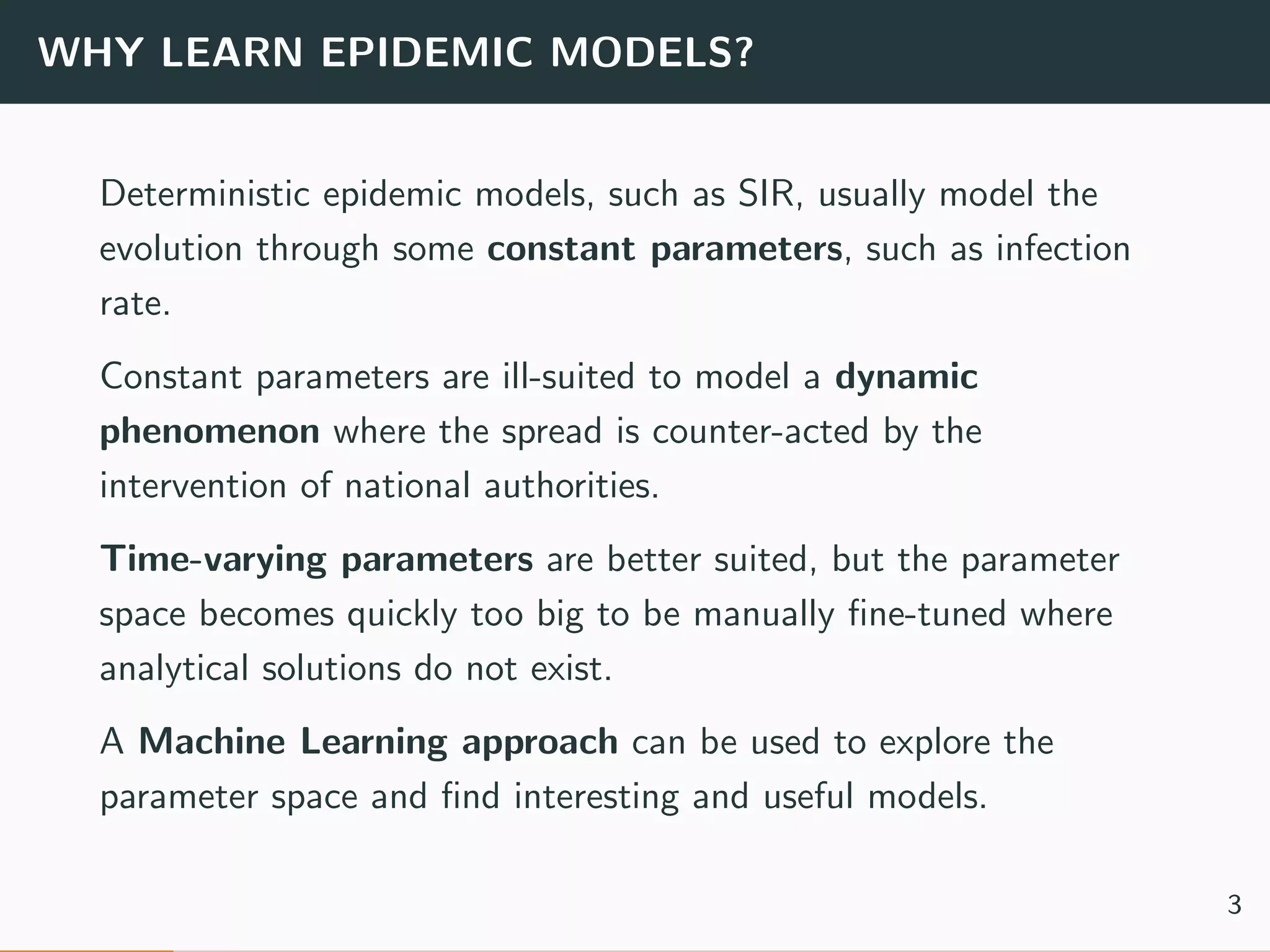
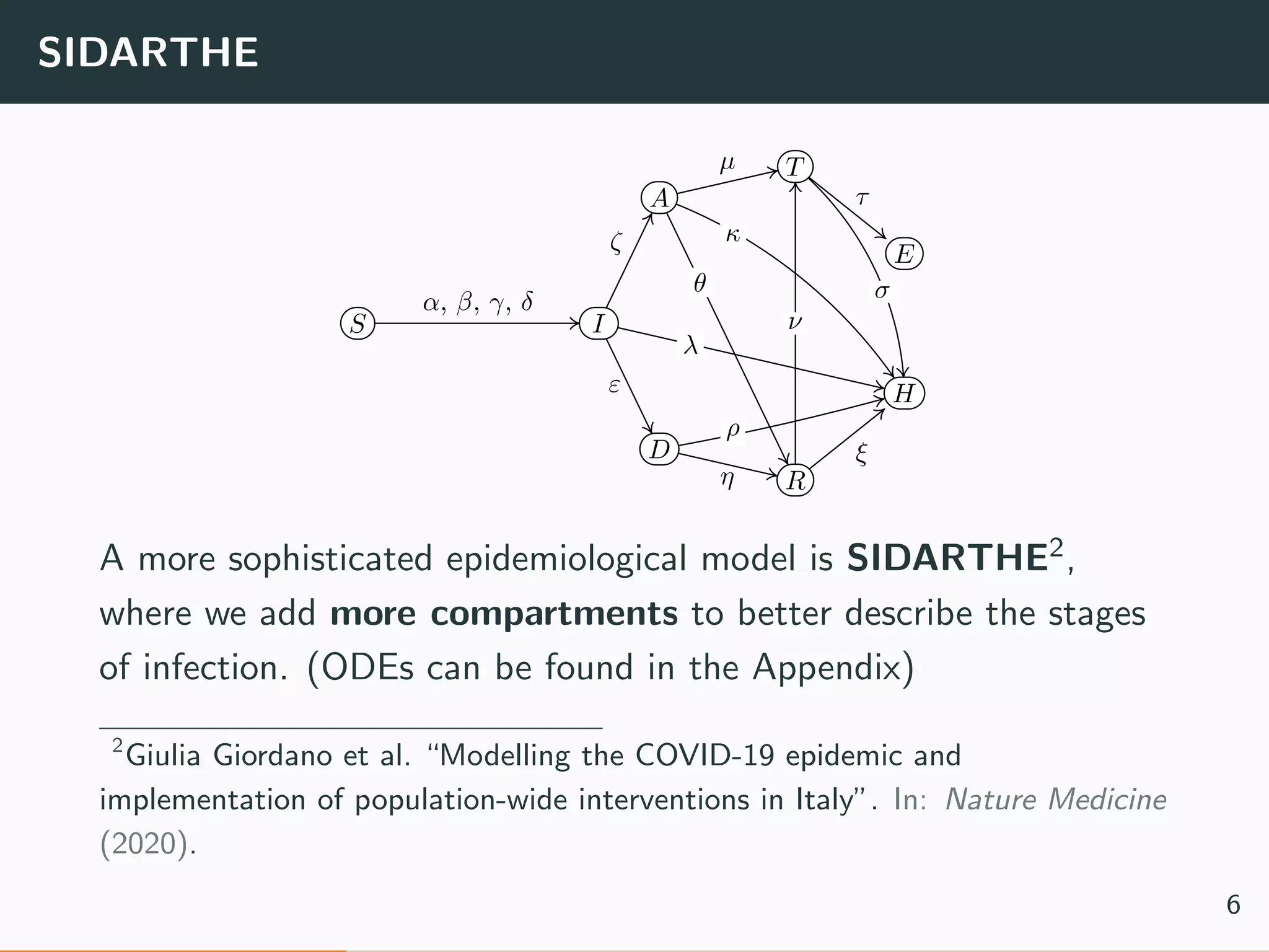
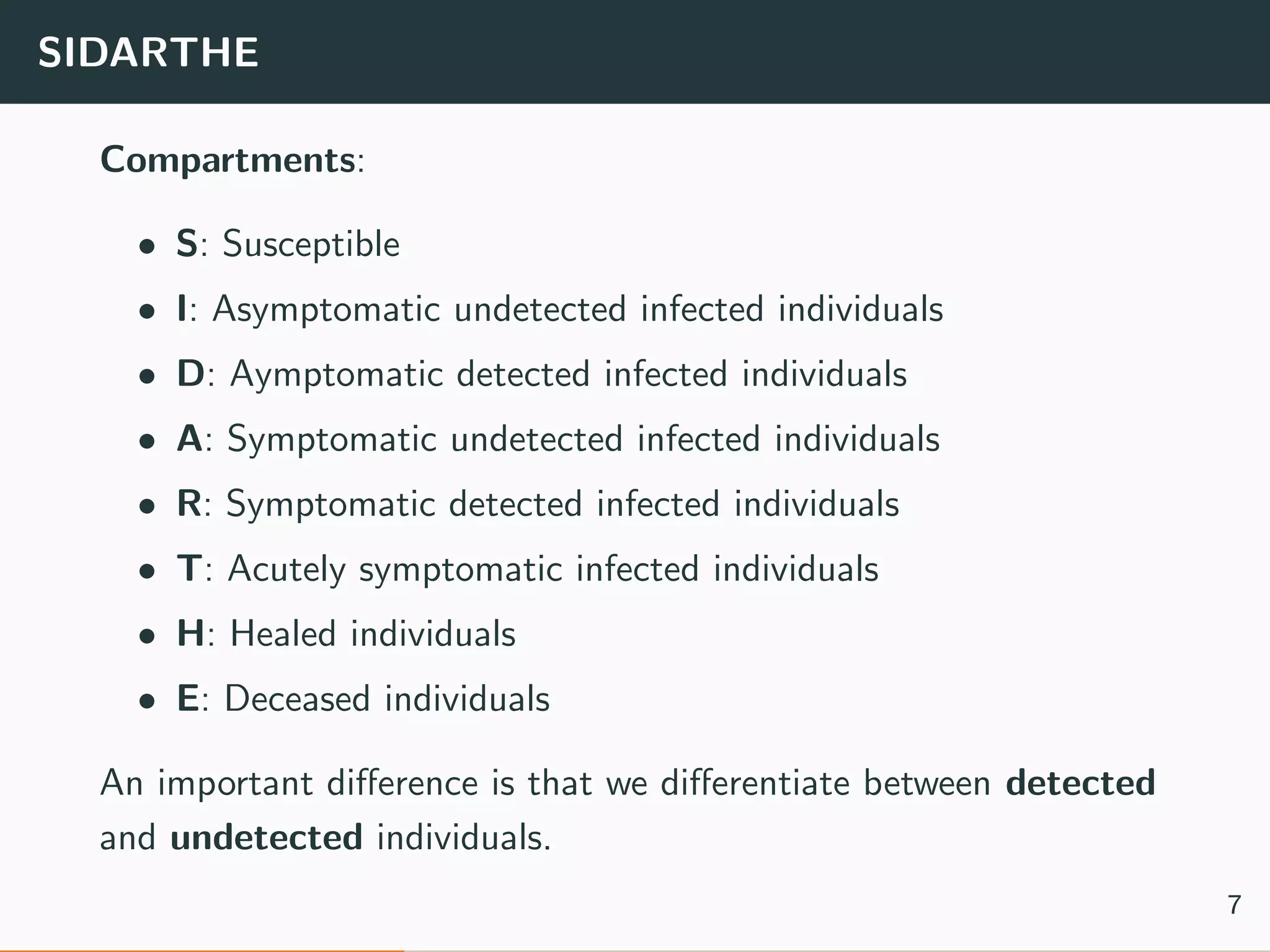
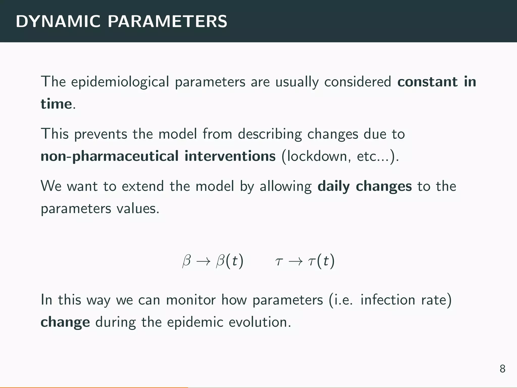
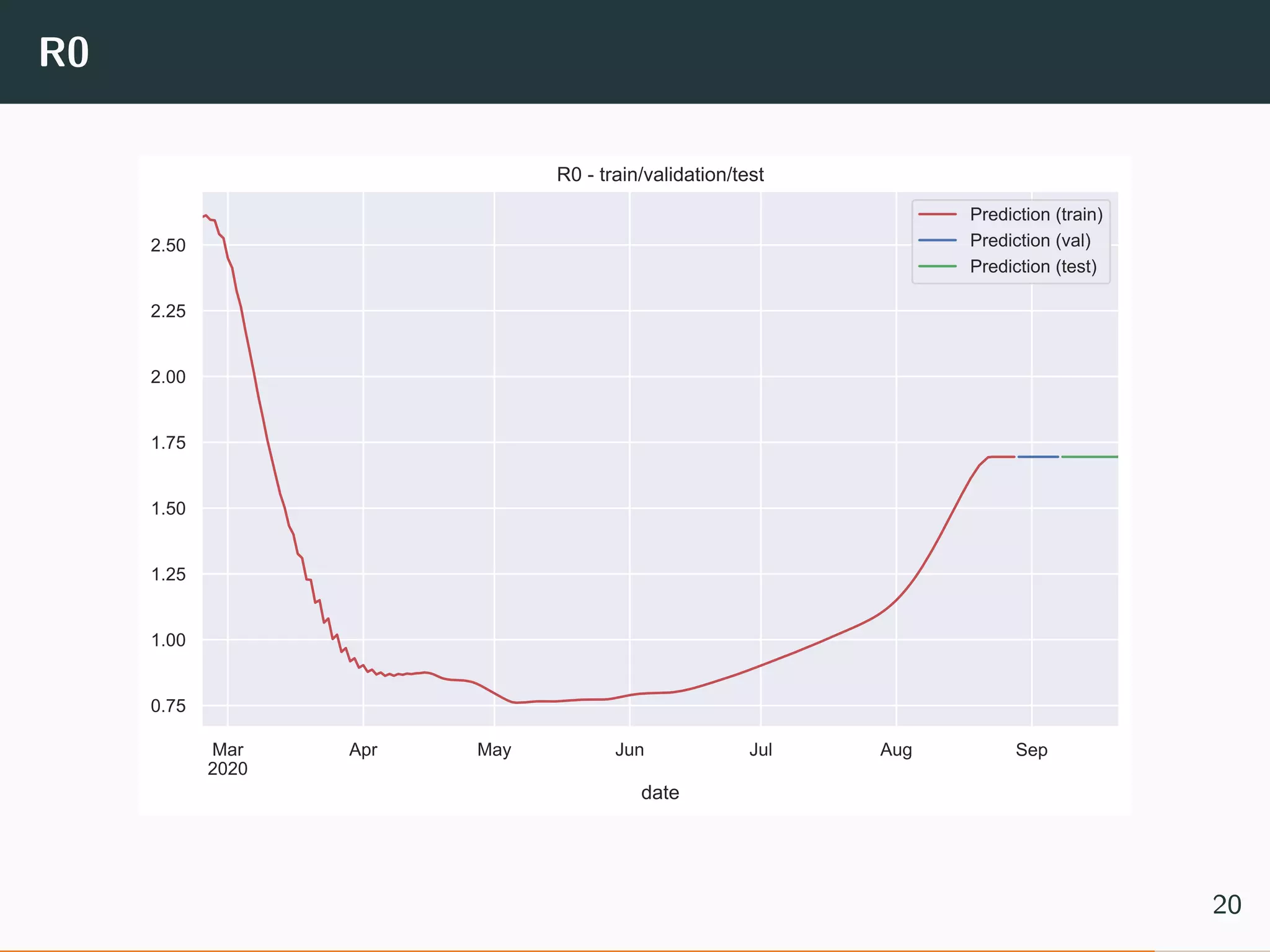
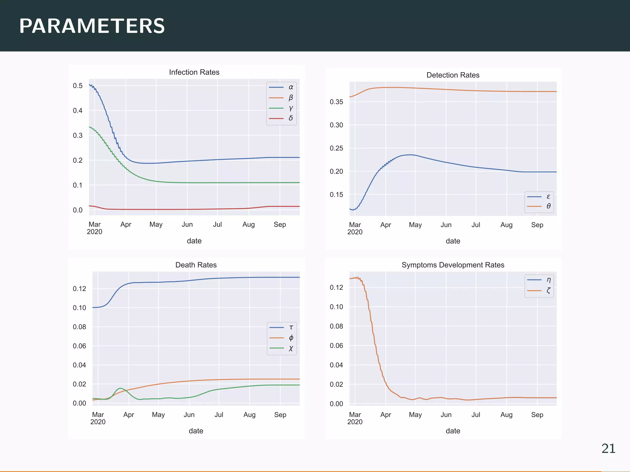
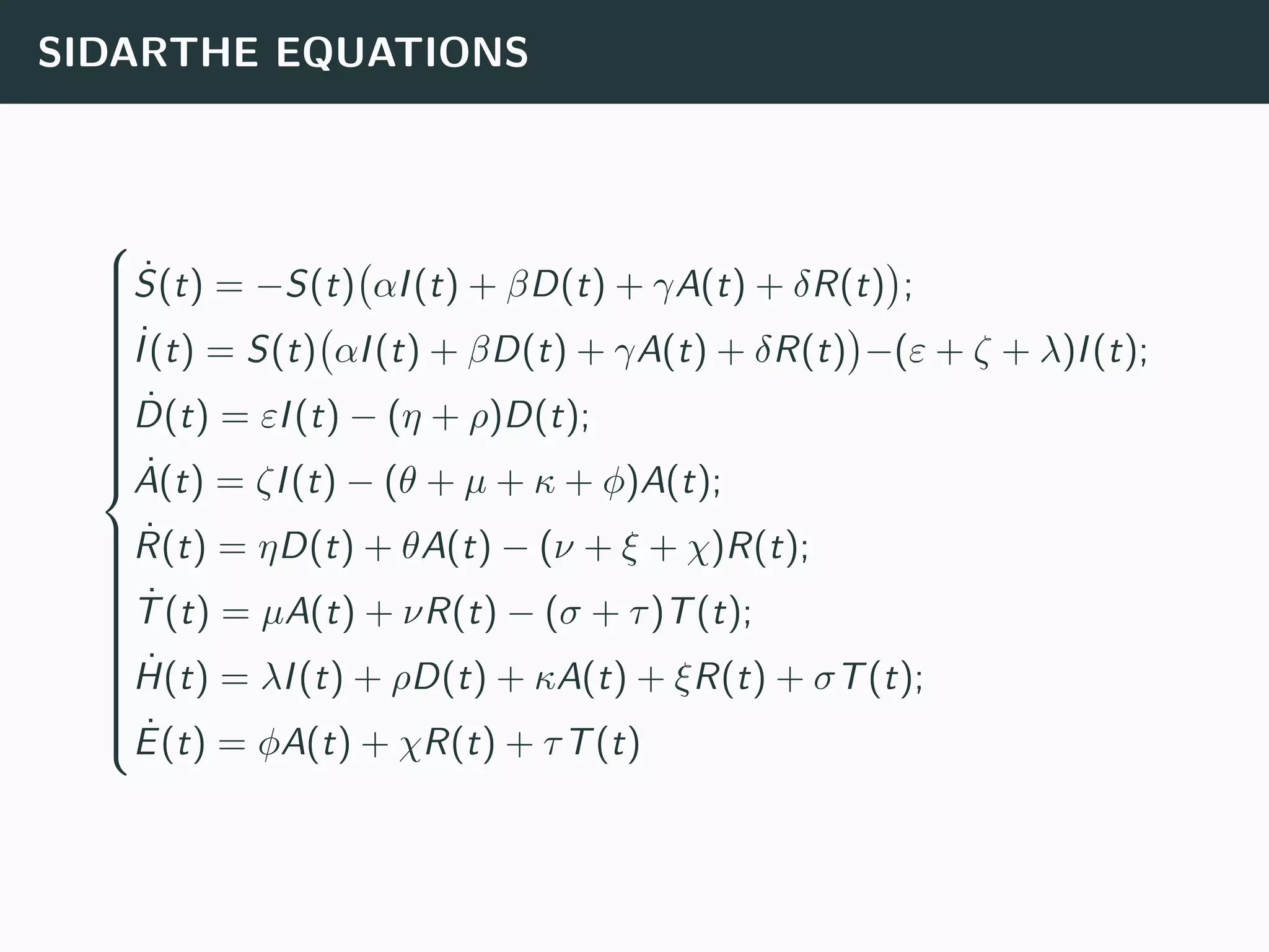
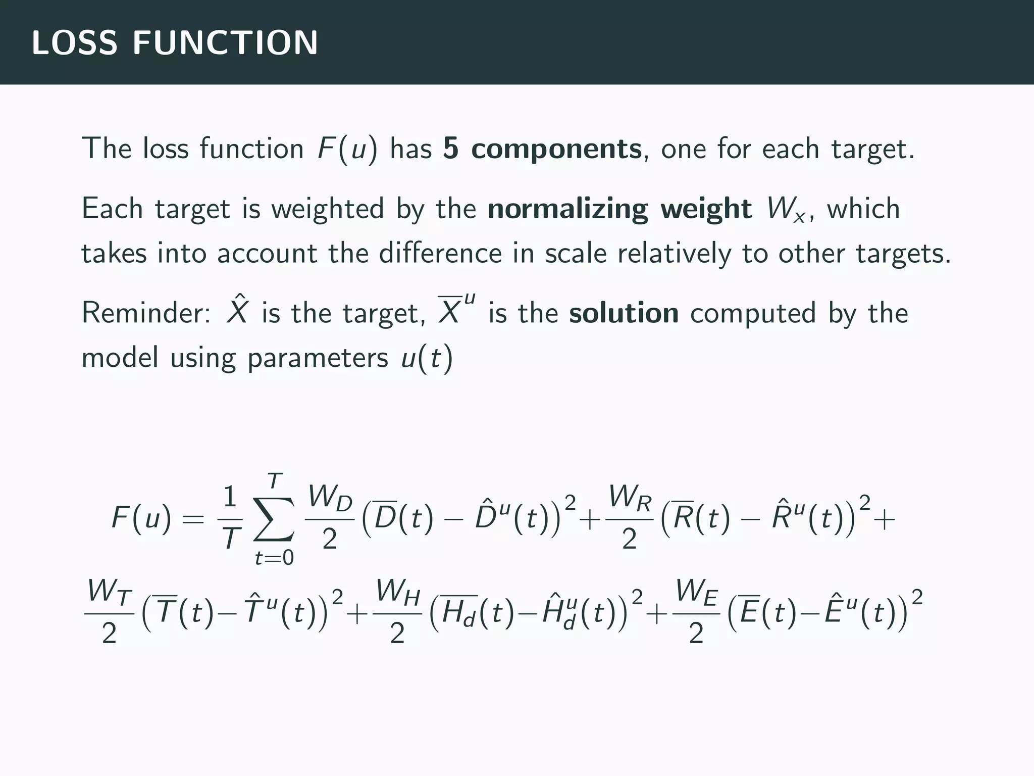
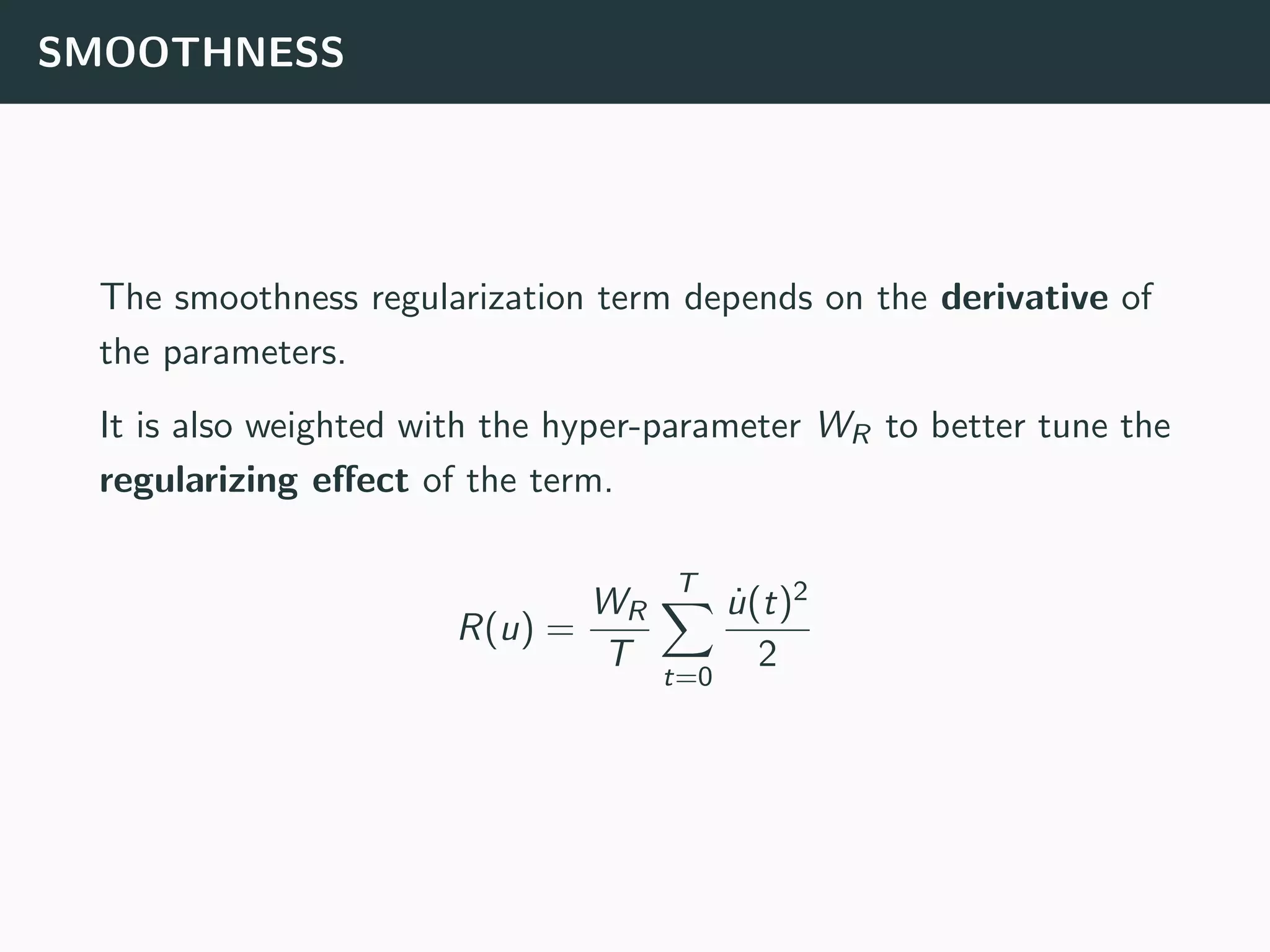
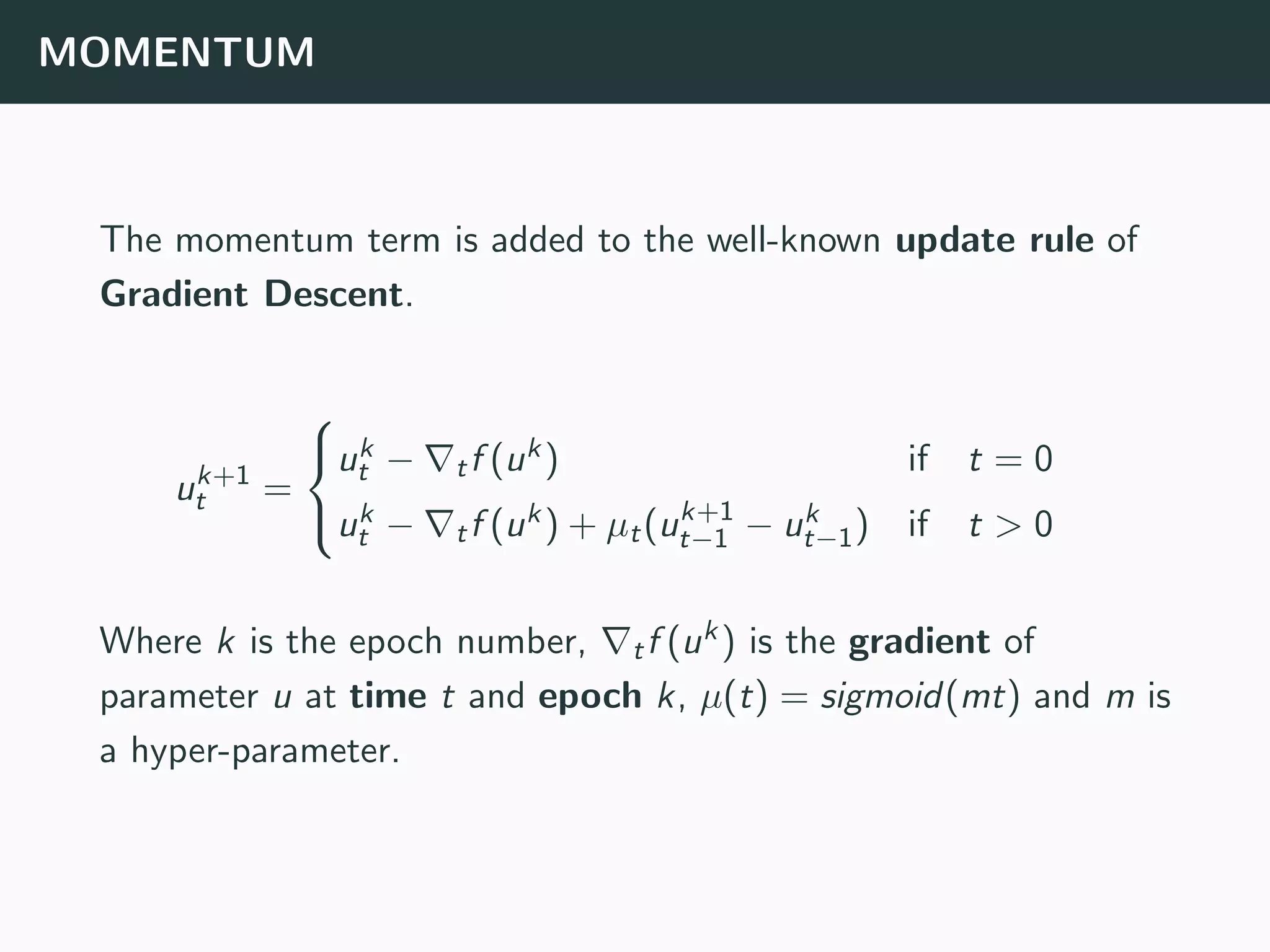
The document discusses the application of machine learning to epidemiological models, particularly in the context of COVID-19. It details the limitations of traditional deterministic models, favoring a more dynamic SIDARTHE model that accommodates time-varying parameters to capture the effects of public health interventions. The document also outlines methodologies for training and validating these models using extensive datasets to better predict the disease spread and evaluate the effectiveness of interventions.

1. MACHINE LEARNING FOR
EPIDEMIOLOGICAL MODELS
E. Meloni, A. Zugarini, A. Panizza, A. Betti, M. Gori
September 24, 2020
SAILab, University of Siena

2. TABLE OF CONTENTS
1. SIR Models
2. The data
3. The learning problem
4. Regularization
5. Fitting the data
1

3. SIR Models

4. WHY LEARN EPIDEMIC MODELS?
During 2020, the spread of COVID-19 infection affected the
whole world.
Some countries resorted to non-pharmaceutical interventions of
various degrees to control the spread of the virus, such as
lockdowns or imposing the use of masks.
Many countries collected vast amounts of detailed data about the
evolution of the epidemic.
Understanding the evolution of the epidemic from the data can
help us understand the efficacy of this interventions and predict
the spread of the illness if no action is taken.
2

5. WHY LEARN EPIDEMIC MODELS?
Deterministic epidemic models, such as SIR, usually model the
evolution through some constant parameters, such as infection
rate.
Constant parameters are ill-suited to model a dynamic
phenomenon where the spread is counter-acted by the
intervention of national authorities.
Time-varying parameters are better suited, but the parameter
space becomes quickly too big to be manually fine-tuned where
analytical solutions do not exist.
A Machine Learning approach can be used to explore the
parameter space and find interesting and useful models.
3

6. THE MODEL
A classical deterministic approach to model an epidemic is the
susceptible, infectious, removed (SIR) model.
A population of N individuals is divided into
• x(t) = (# of susceptible at time t)
• y(t) = (# of infectious at time t)
• z(t) = (# of removed at time t)
We assume that the population remains constant, therefore:
x(t) + y(t) + z(t) = N.
4

7. THE MODEL
The dynamics of the epidemics then can be described by the
following system of ODEs1:



x (t) = −βx(t)y(t)
y (t) = βx(t)y(t) − γy(t)
z (t) = γy(t)
• β > 0 → infection rate
• γ > 0 → removal rate
• R0 := β/γ → reproduction number
1
Norman TJ Bailey et al. The mathematical theory of infectious diseases and
its applications. Charles Griffin & Company Ltd, 1975.
5

8. SIDARTHE
S I
D
R
H
E
T
A
α, β, γ, δ
ε
η
ξ
ζ
µ
τ
ρ
λ
κ
ν
σθ
A more sophisticated epidemiological model is SIDARTHE2,
where we add more compartments to better describe the stages
of infection. (ODEs can be found in the Appendix)
2
Giulia Giordano et al. “Modelling the COVID-19 epidemic and
implementation of population-wide interventions in Italy”. In: Nature Medicine
(2020).
6

9. SIDARTHE
Compartments:
• S: Susceptible
• I: Asymptomatic undetected infected individuals
• D: Aymptomatic detected infected individuals
• A: Symptomatic undetected infected individuals
• R: Symptomatic detected infected individuals
• T: Acutely symptomatic infected individuals
• H: Healed individuals
• E: Deceased individuals
An important difference is that we differentiate between detected
and undetected individuals.
7

10. DYNAMIC PARAMETERS
The epidemiological parameters are usually considered constant in
time.
This prevents the model from describing changes due to
non-pharmaceutical interventions (lockdown, etc...).
We want to extend the model by allowing daily changes to the
parameters values.
β → β(t) τ → τ(t)
In this way we can monitor how parameters (i.e. infection rate)
change during the epidemic evolution.
8

11. The data

12. OFFICIAL DATA
We pre-processed the data3 to obtain 5 time-series which map to
5 SIDARTHE compartments:
• D: detected asymptomatic individuals
• R: detected symptomatic individuals
• T: acutely symptomatic individuals
• Hd : portion of healed individuals that were previously detected
• E: deceased individuals
We do not have access to data about the undetected infected
individuals (of course).
3
You can find the data following this link:
https://github.com/pcm-dpc/COVID-19
9

13. TRAIN/VALIDATION/TEST SPLIT
All time-series were split into three sets:
• Train Set (size T): 0 ≤ t ≤ T
• Validation Set (size V): T ≤ t ≤ T + V
• Test Set (size D): T + V ≤ t ≤ T + V + D
As usual, the training set will be used to fit the model, the
validation set will be used to evaluate over-fitting and the test set
will be used for the final evaluation of the model.
10

14. The learning problem

15. GENERIC STATEMENT
We call u(t) the concatenation of all parameters at time t.
u(t) = (α(t), β(t)...)
Problem
Learning u(t) from supervisions on the number of people in the
detected compartments, i.e. D, R, T, Hd and E.
11

16. PRECISE FORMULATION
Given the supervisions D, R, T, Hd and E
Given ˆDu, ˆRu, ˆTu, ˆHu
d and ˆEu the solutions of SIDARTHE
equations given by parameters u(t).
We want to find the set of parameters u(t) which minimizes the
MSE of the prediction against the targets on samples for
t = 0 → T.
12

17. GRADIENT DESCENT THROUGH ODES
The learning is done through Gradient Descent.
The SIDARTHE equations are computed through numeric
integration, using Heun method and a fixed time step.
To obtain the gradient of parameters through the integration, we
have implemented the Heun method in PyTorch to leverage its
powerful autograd framework.
Sidenote: there are strong similarities with Neural ODEs.
13

18. Regularization

19. SMOOTHNESS
In case of overfitting, the learned parameters could result in a
discontinuous and wrinkled function of time.
To avoid this problem and reduce overfitting, we augment the loss
function with a regularization term R(u).
The penalty R(u) is higher when the parameters are discontinuous
and enforces a smooth function.
14

20. MOMENTUM
Since the solution is computed through integration, the value of
parameters at initial time steps have a bigger impact on the
solution w.r.t. values at final time steps.
This can be seen in the gradient of each parameter: for t → T,
gradients approach 0.
Hence, we augmented the Gradient Descent update rule with a
momentum term, which manages to distribute the gradient
throughout the u function.
Important note: the commonly known momentum carries the
gradient over subsequent epochs; this momentum term carries the
gradient over subsequent time steps of the parameters u(t)
15

21. TARGET NORMALIZATION
D, R, T, Hd and E have very different scales of values.
E.g. max(Hd ) ≈ 200 000 and max(T) ≈ 4 000
This could cause the learning to prefer a target at the expense of
another one.
We weight the loss components for each target based on its scale
relative to the other targets.
16

22. Fitting the data

23. INFECTED INDIVIDUALS
0DU
$SU 0D -XQ -XO $XJ 6HS
GDWH
'WUDLQYDOLGDWLRQWHVW
3UHGLFWLRQWUDLQ

24. 7DUJHWWUDLQ

25. 3UHGLFWLRQYDO

26. 7DUJHWYDO

27. 3UHGLFWLRQWHVW

28. 7DUJHWWHVW

29. 0DU
$SU 0D -XQ -XO $XJ 6HS
GDWH
5WUDLQYDOLGDWLRQWHVW
3UHGLFWLRQWUDLQ

30. 7DUJHWWUDLQ

31. 3UHGLFWLRQYDO

32. 7DUJHWYDO

33. 3UHGLFWLRQWHVW

34. 7DUJHWWHVW

35. 17

36. ACUTELY SYMPTOMATIC DECEASED
0DU
$SU 0D -XQ -XO $XJ 6HS
GDWH
7WUDLQYDOLGDWLRQWHVW
3UHGLFWLRQWUDLQ

37. 7DUJHWWUDLQ

38. 3UHGLFWLRQYDO

39. 7DUJHWYDO

40. 3UHGLFWLRQWHVW

41. 7DUJHWWHVW

42. 0DU
$SU 0D -XQ -XO $XJ 6HS
GDWH
(WUDLQYDOLGDWLRQWHVW
3UHGLFWLRQWUDLQ

43. 7DUJHWWUDLQ

44. 3UHGLFWLRQYDO

45. 7DUJHWYDO

46. 3UHGLFWLRQWHVW

47. 7DUJHWWHVW

48. 18

49. DETECTED HEALED INDIVIDUALS
0DU
$SU 0D -XQ -XO $XJ 6HS
GDWH
+B'(7(7('WUDLQYDOLGDWLRQWHVW
3UHGLFWLRQWUDLQ

50. 7DUJHWWUDLQ

51. 3UHGLFWLRQYDO

52. 7DUJHWYDO

53. 3UHGLFWLRQWHVW

54. 7DUJHWWHVW

55. 19

56. R0
0DU
$SU 0D -XQ -XO $XJ 6HS
GDWH
5WUDLQYDOLGDWLRQWHVW
3UHGLFWLRQWUDLQ

57. 3UHGLFWLRQYDO

58. 3UHGLFWLRQWHVW

59. 20

60. PARAMETERS
0DU
$SU 0D -XQ -XO $XJ 6HS
GDWH
,QIHFWLRQ5DWHV
0DU
$SU 0D -XQ -XO $XJ 6HS
GDWH
'HWHFWLRQ5DWHV
0DU
$SU 0D -XQ -XO $XJ 6HS
GDWH
'HDWK5DWHV
0DU
$SU 0D -XQ -XO $XJ 6HS
GDWH
6PSWRPV'HYHORSPHQW5DWHV
21

61. Thank you for listening!
21

62. References
Bailey, Norman TJ et al. The mathematical theory of infectious diseases
and its applications. Charles Griffin Company Ltd, 1975.
Giordano, Giulia et al. “Modelling the COVID-19 epidemic and
implementation of population-wide interventions in Italy”. In: Nature
Medicine (2020).
22

63. Appendix

64. SIDARTHE EQUATIONS



˙S(t) = −S(t) αI(t) + βD(t) + γA(t) + δR(t) ;
˙I(t) = S(t) αI(t) + βD(t) + γA(t) + δR(t) −(ε + ζ + λ)I(t);
˙D(t) = εI(t) − (η + ρ)D(t);
˙A(t) = ζI(t) − (θ + µ + κ + φ)A(t);
˙R(t) = ηD(t) + θA(t) − (ν + ξ + χ)R(t);
˙T(t) = µA(t) + νR(t) − (σ + τ)T(t);
˙H(t) = λI(t) + ρD(t) + κA(t) + ξR(t) + σT(t);
˙E(t) = φA(t) + χR(t) + τT(t)

65. LOSS FUNCTION
The loss function F(u) has 5 components, one for each target.
Each target is weighted by the normalizing weight Wx , which
takes into account the difference in scale relatively to other targets.
Reminder: ˆX is the target, X
u
is the solution computed by the
model using parameters u(t)
F(u) =
1
T
T
t=0
WD
2
D(t) − ˆDu
(t)
2
+
WR
2
R(t) − ˆRu
(t)
2
+
WT
2
T(t)− ˆTu
(t)
2
+
WH
2
Hd (t)− ˆHu
d (t)
2
+
WE
2
E(t)− ˆEu
(t)
2

66. SMOOTHNESS
The smoothness regularization term depends on the derivative of
the parameters.
It is also weighted with the hyper-parameter WR to better tune the
regularizing effect of the term.
R(u) =
WR
T
T
t=0
˙u(t)2
2

67. MOMENTUM
The momentum term is added to the well-known update rule of
Gradient Descent.
uk+1
t =



uk
t − tf (uk) if t = 0
uk
t − tf (uk) + µt(uk+1
t−1 − uk
t−1) if t 0
Where k is the epoch number, tf (uk) is the gradient of
parameter u at time t and epoch k, µ(t) = sigmoid(mt) and m is
a hyper-parameter.

68. LINKS
SAILab: https://sailab.diism.unisi.it/
Code: https://github.com/sailab-code/learning-sidarthe
Data: https://github.com/pcm-dpc/COVID-19
Speaker webpage: https://enricomeloni.github.io