PPT, PDF9,223 views

Surface finish metrology iss1

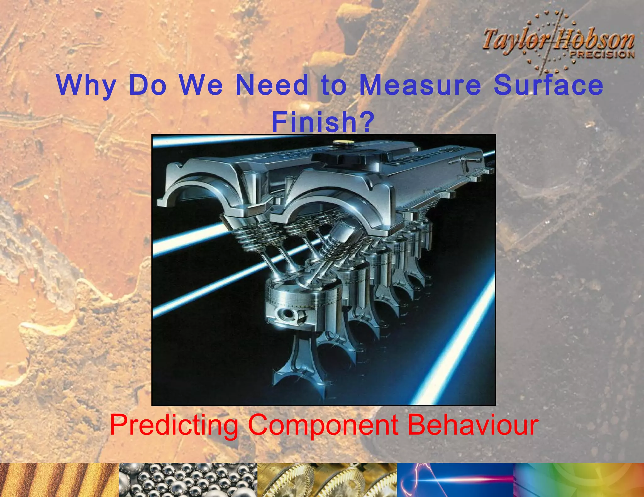
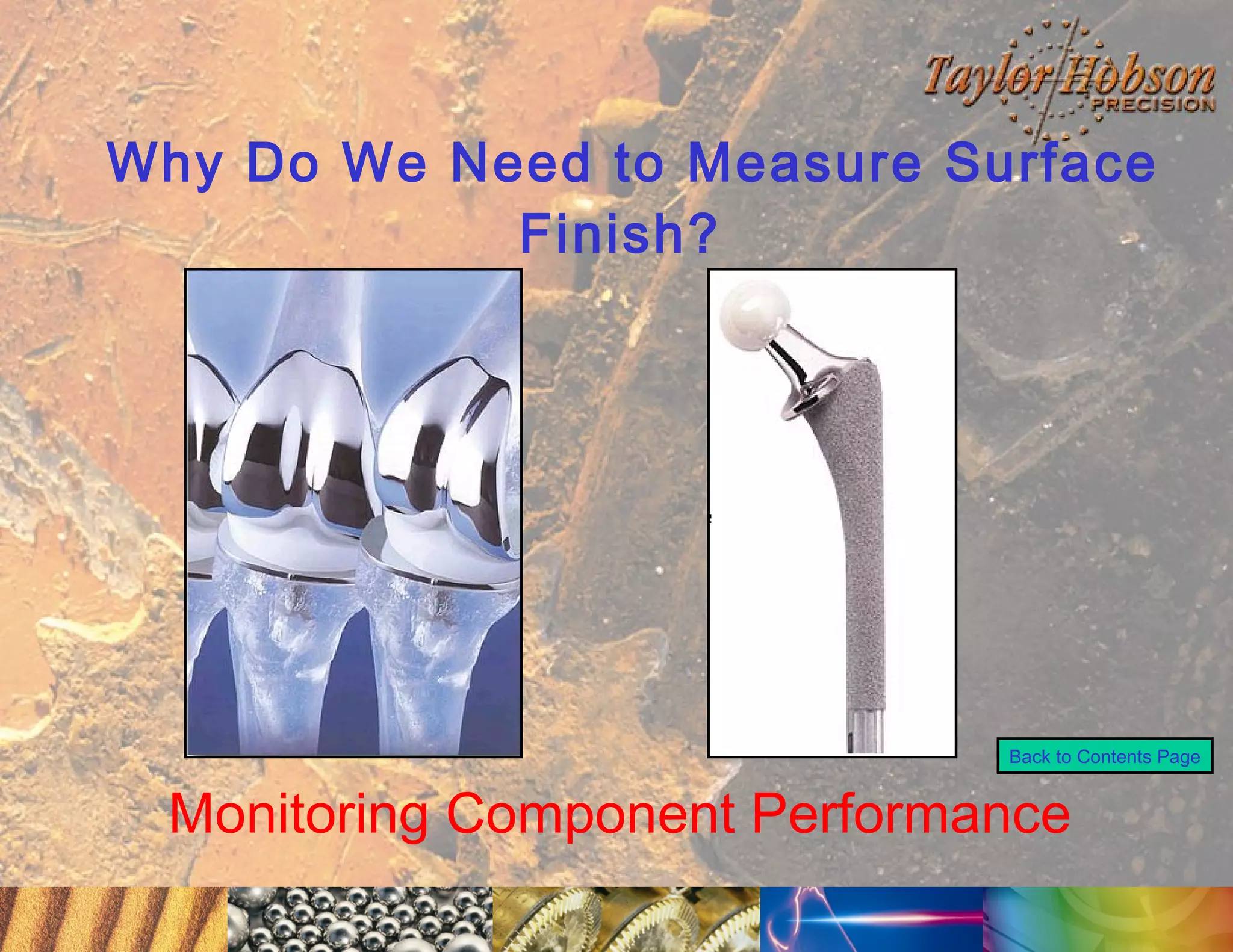
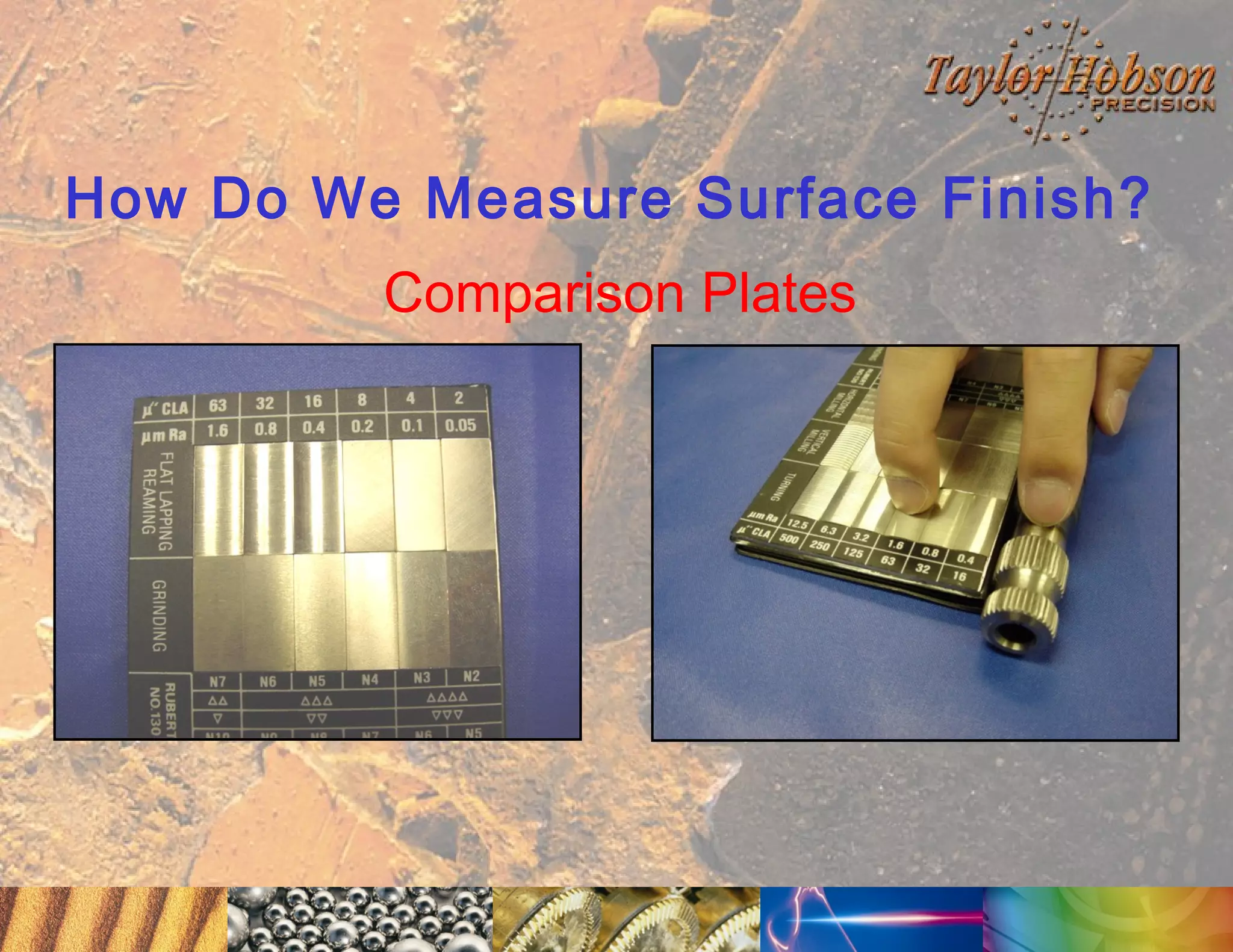
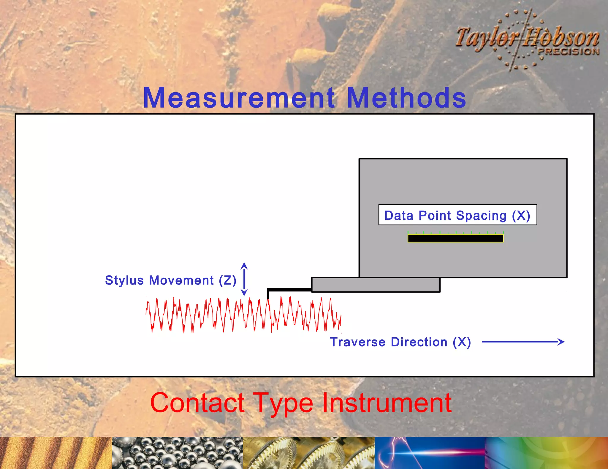
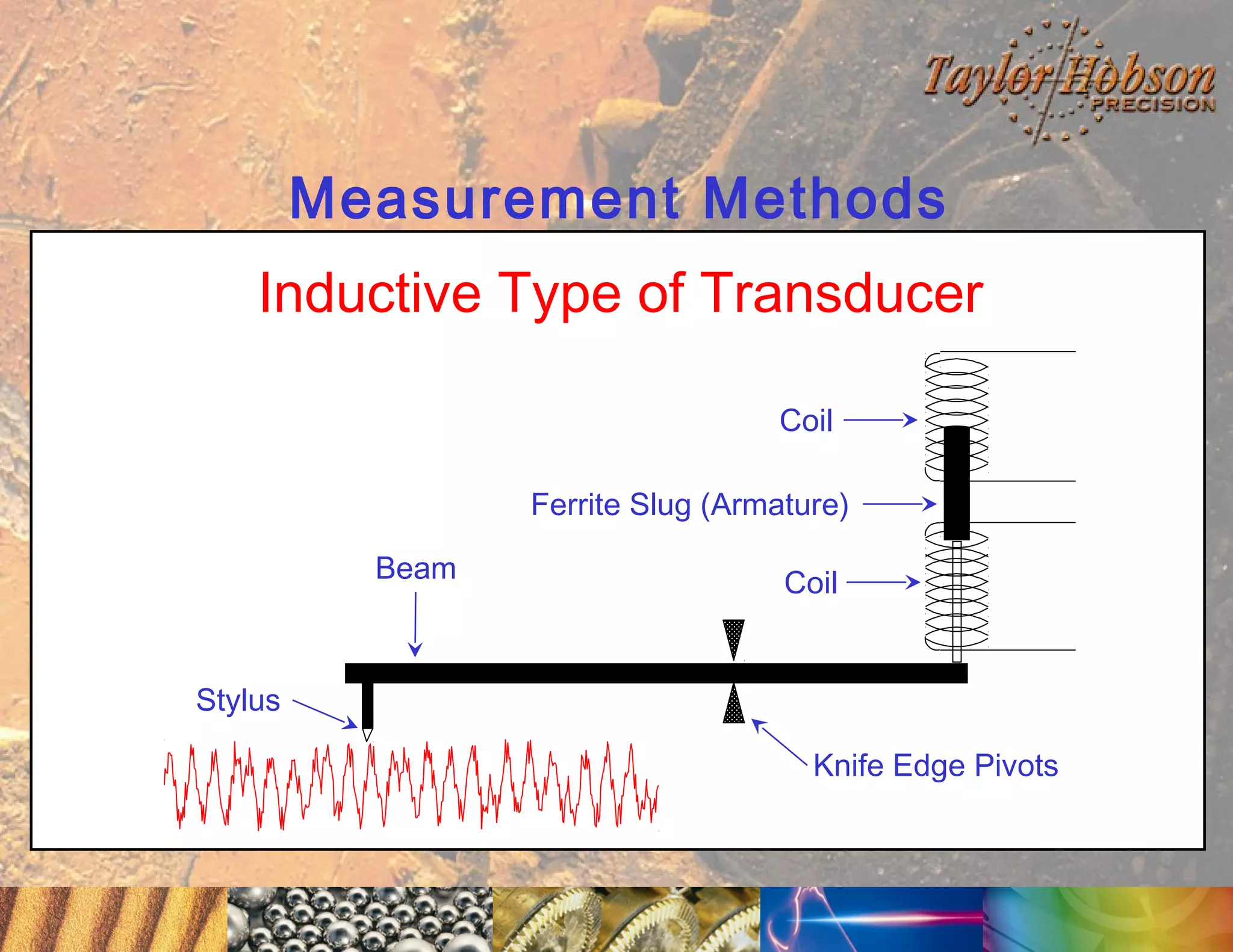
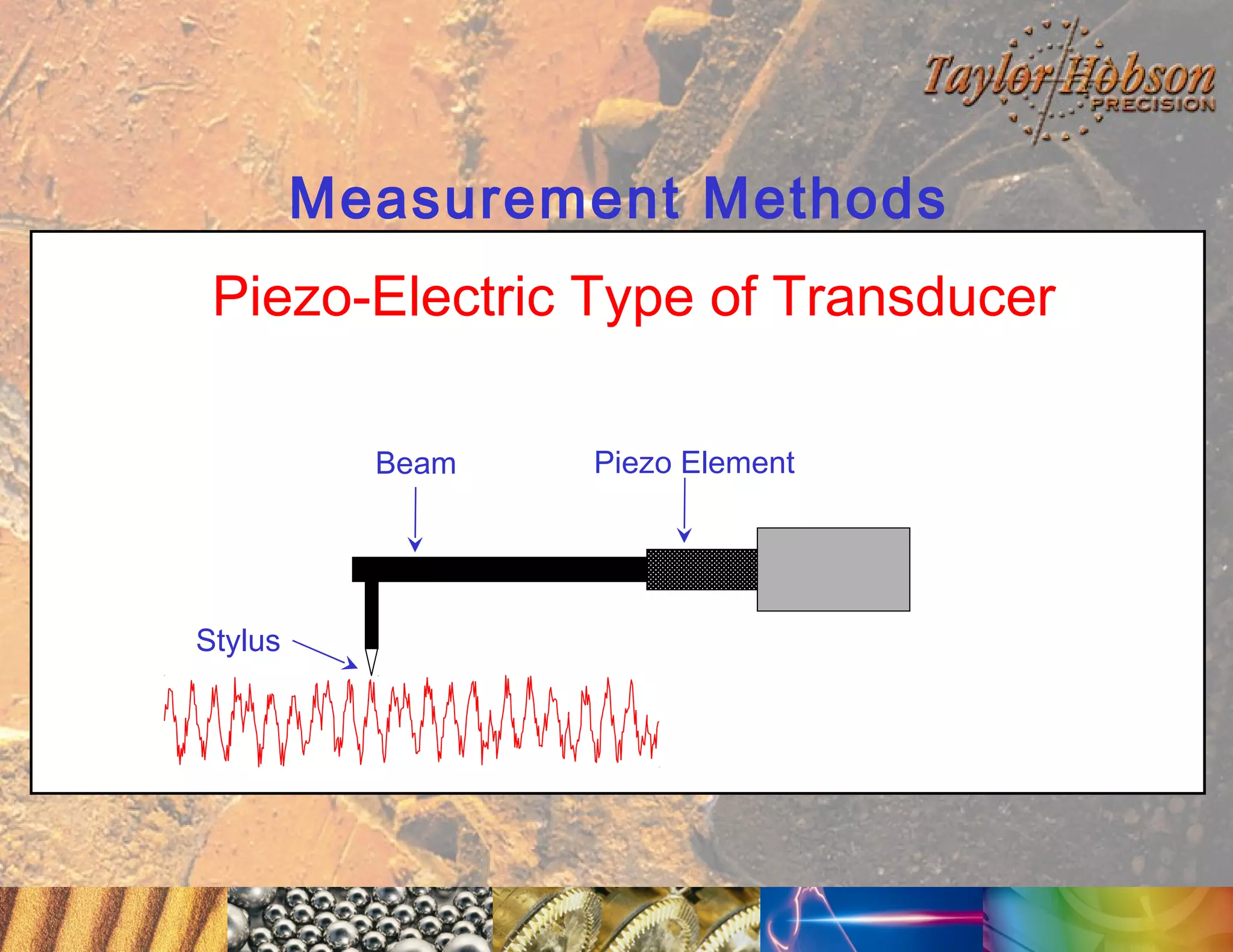
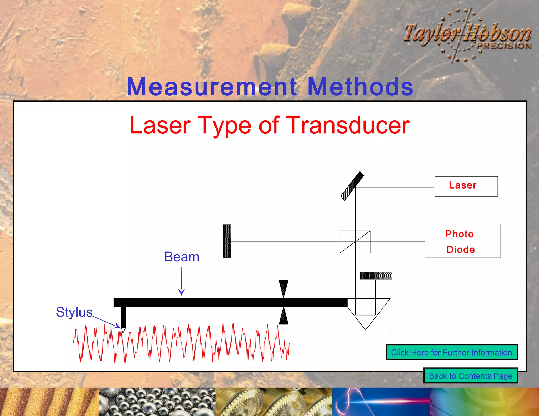
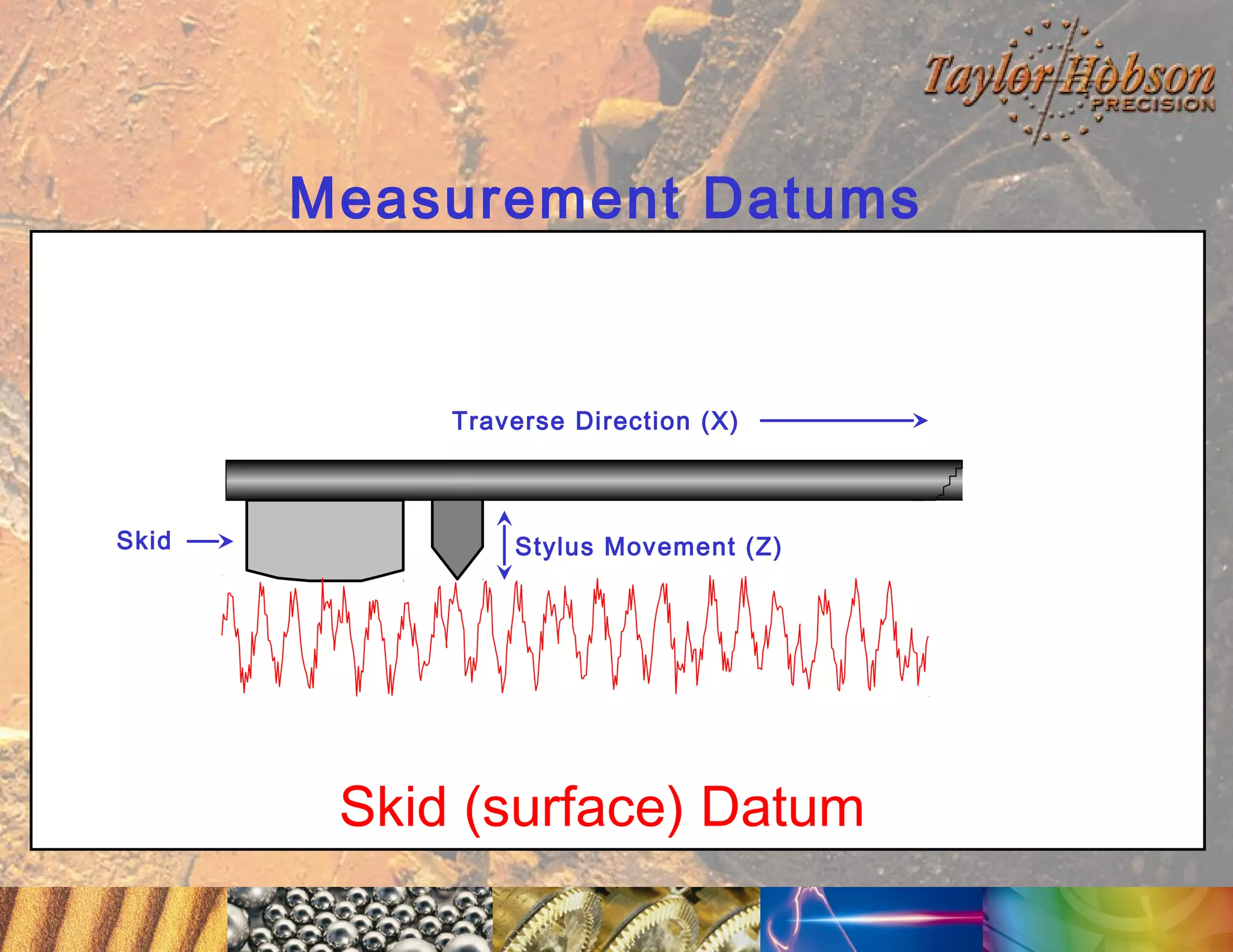
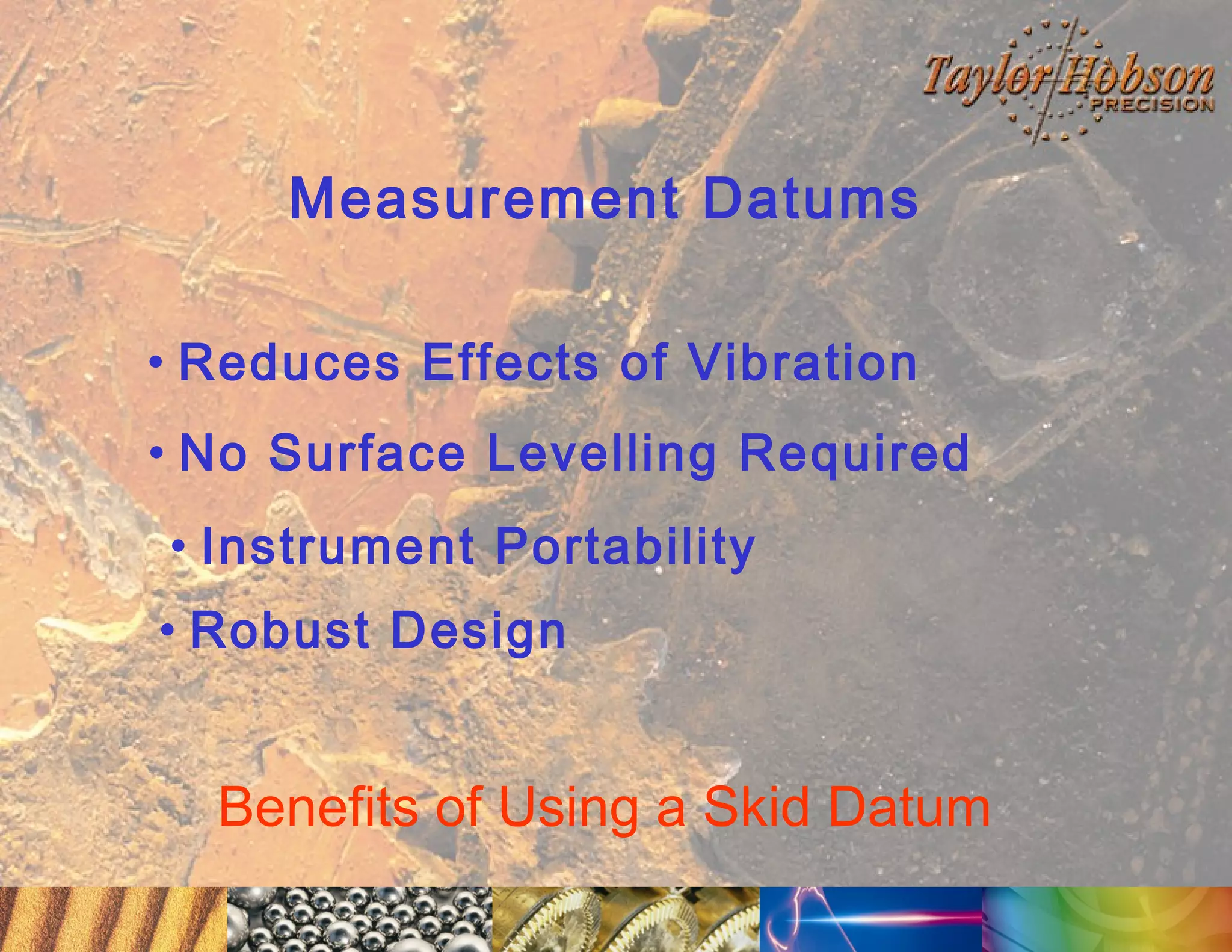
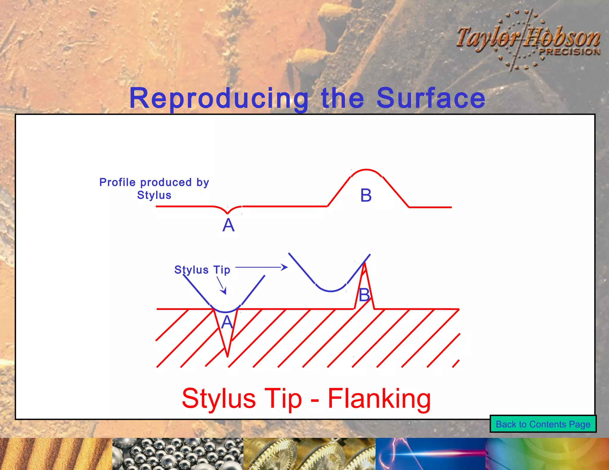
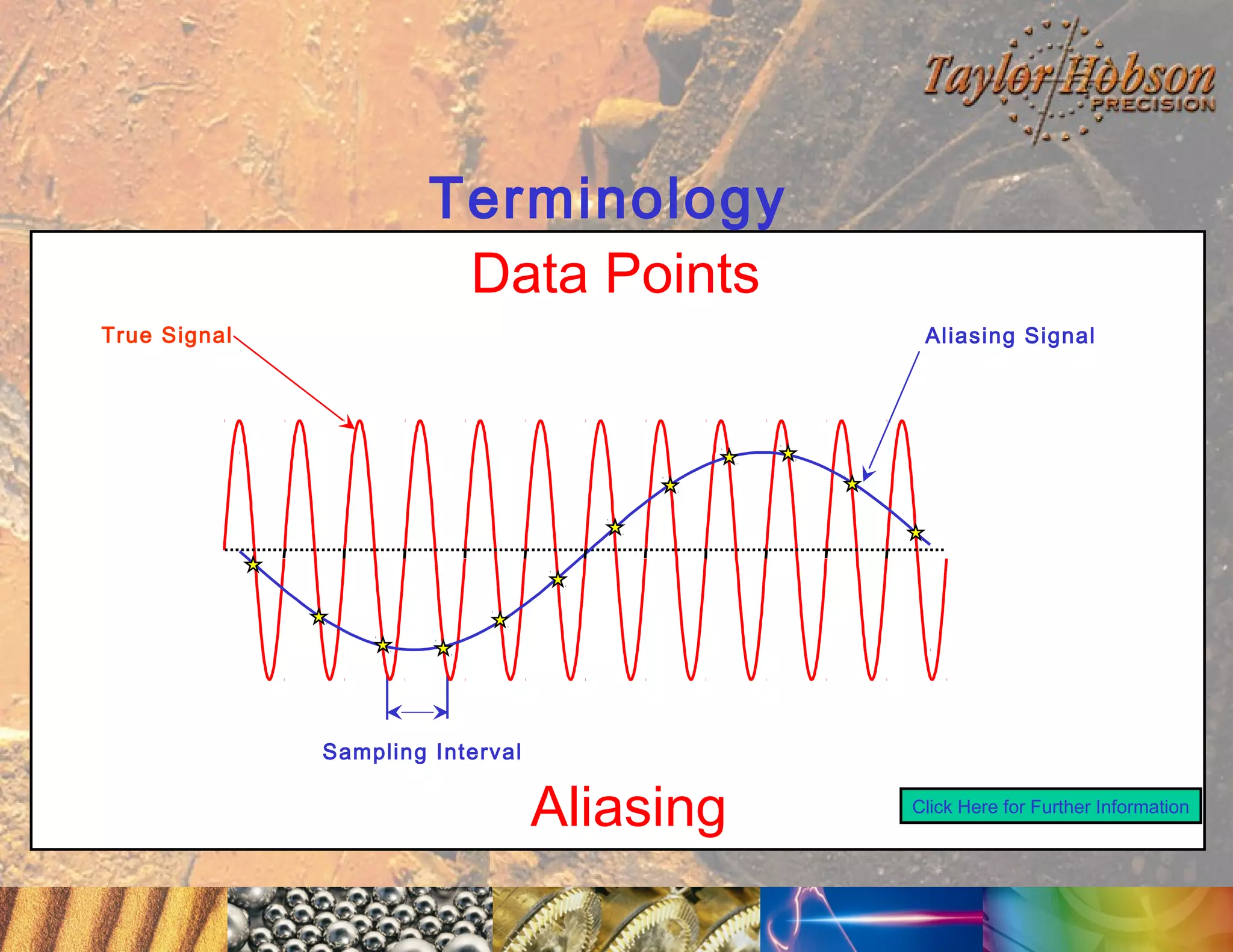
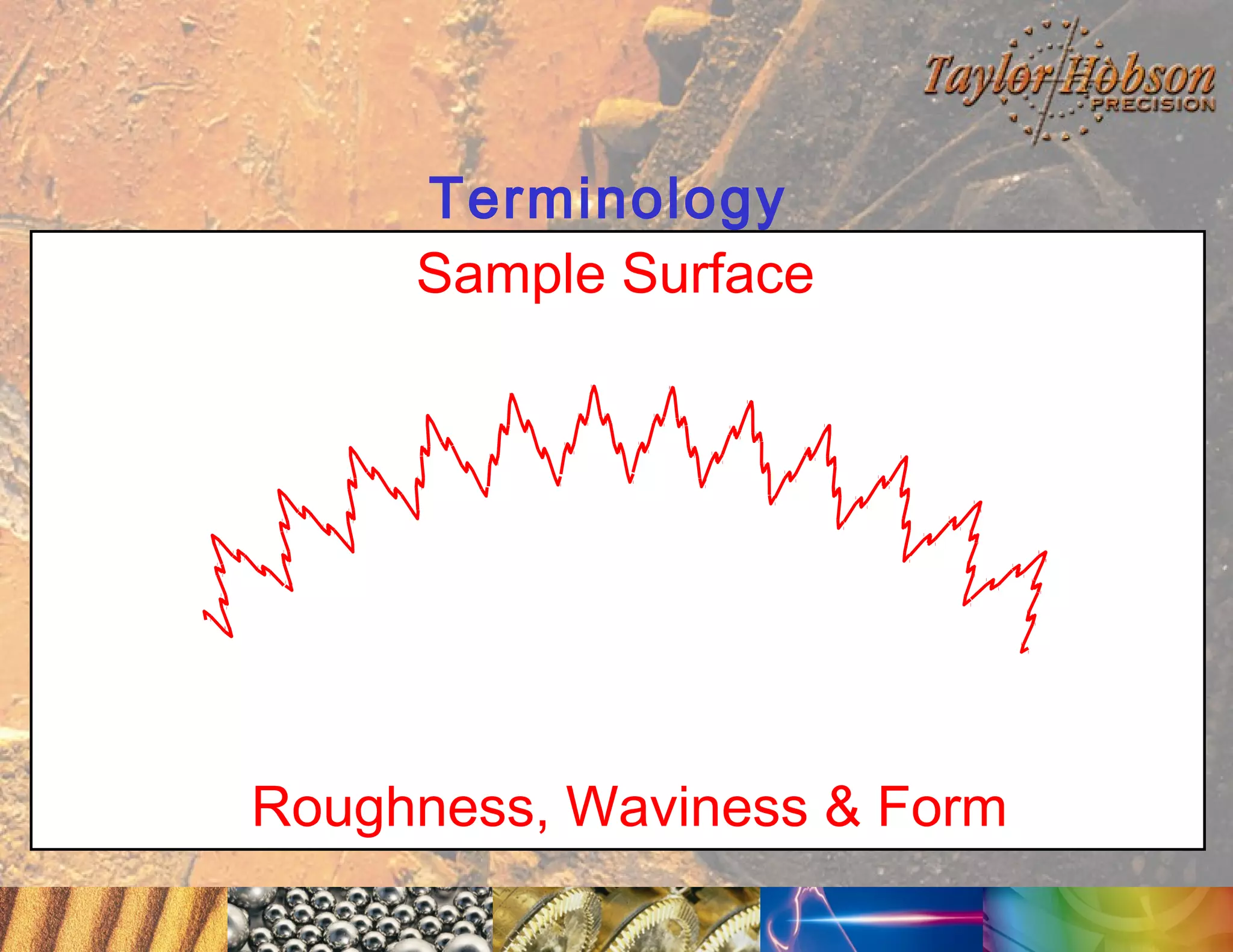
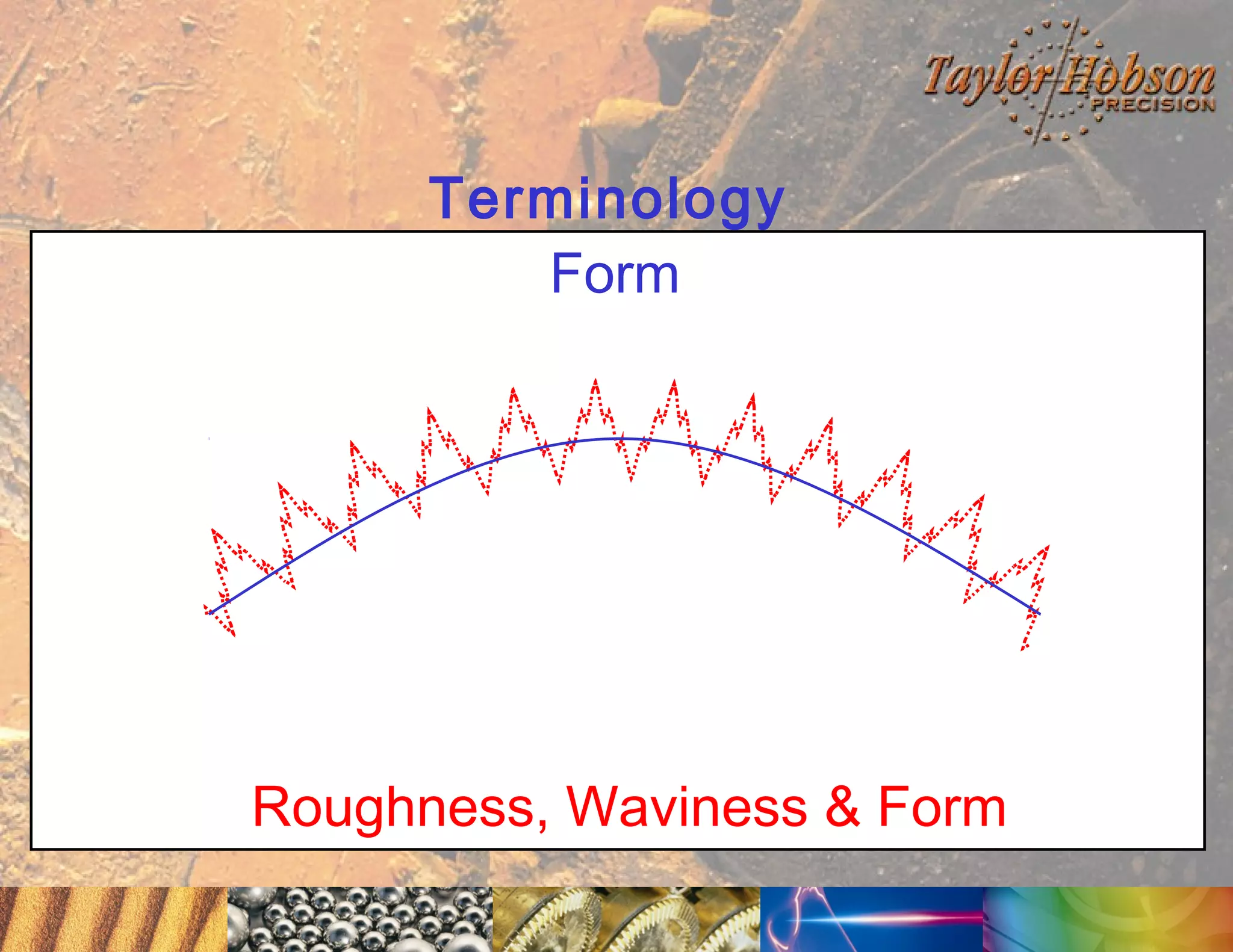
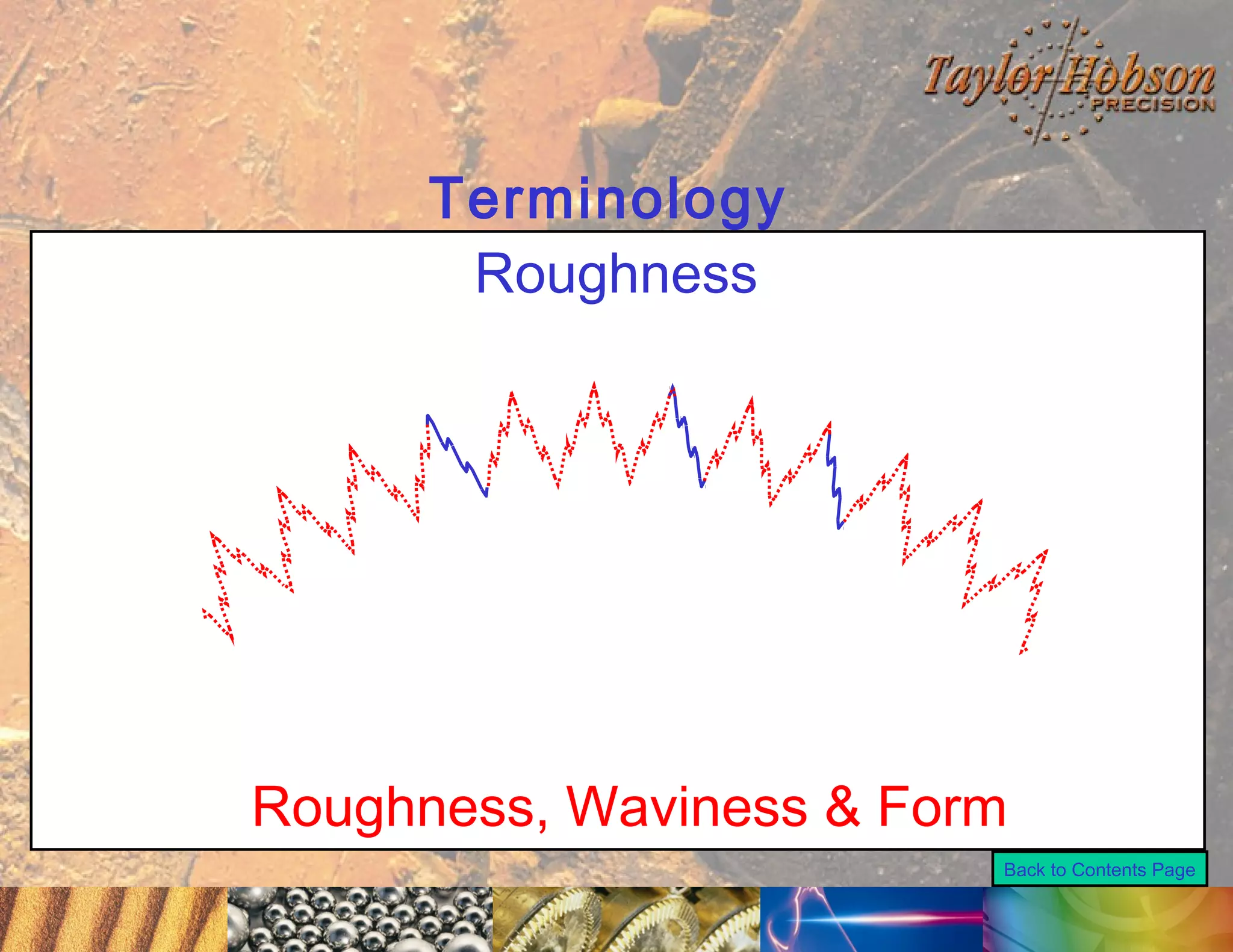
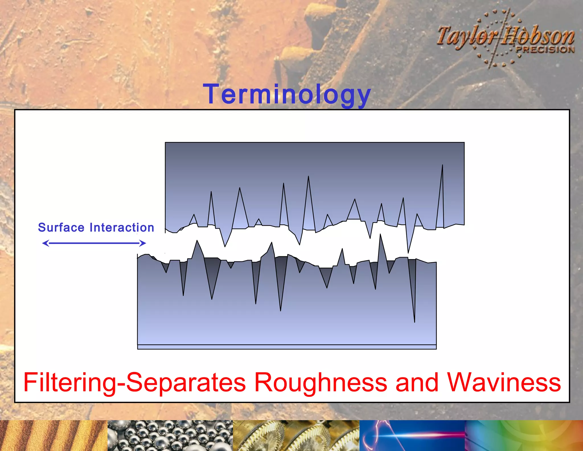
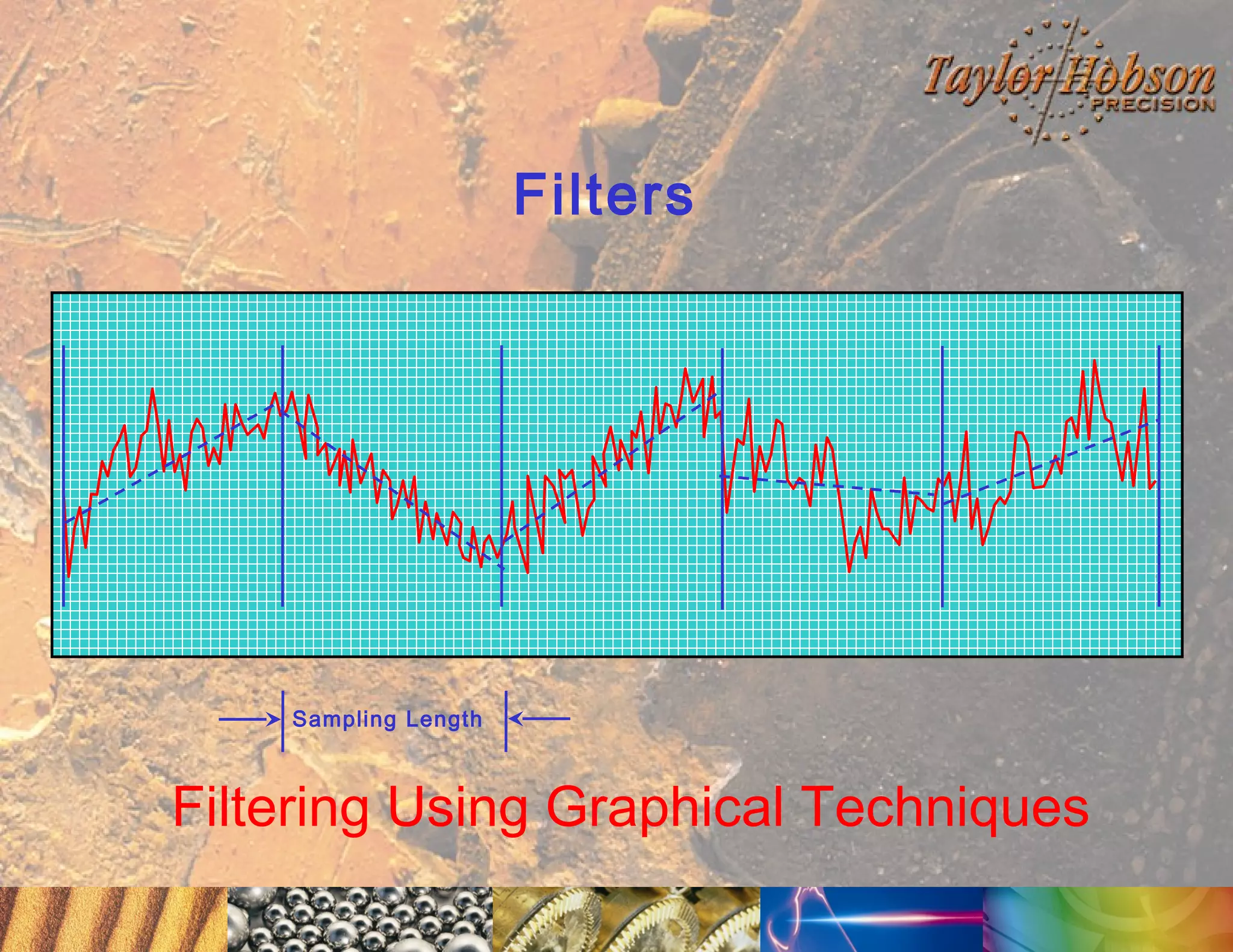
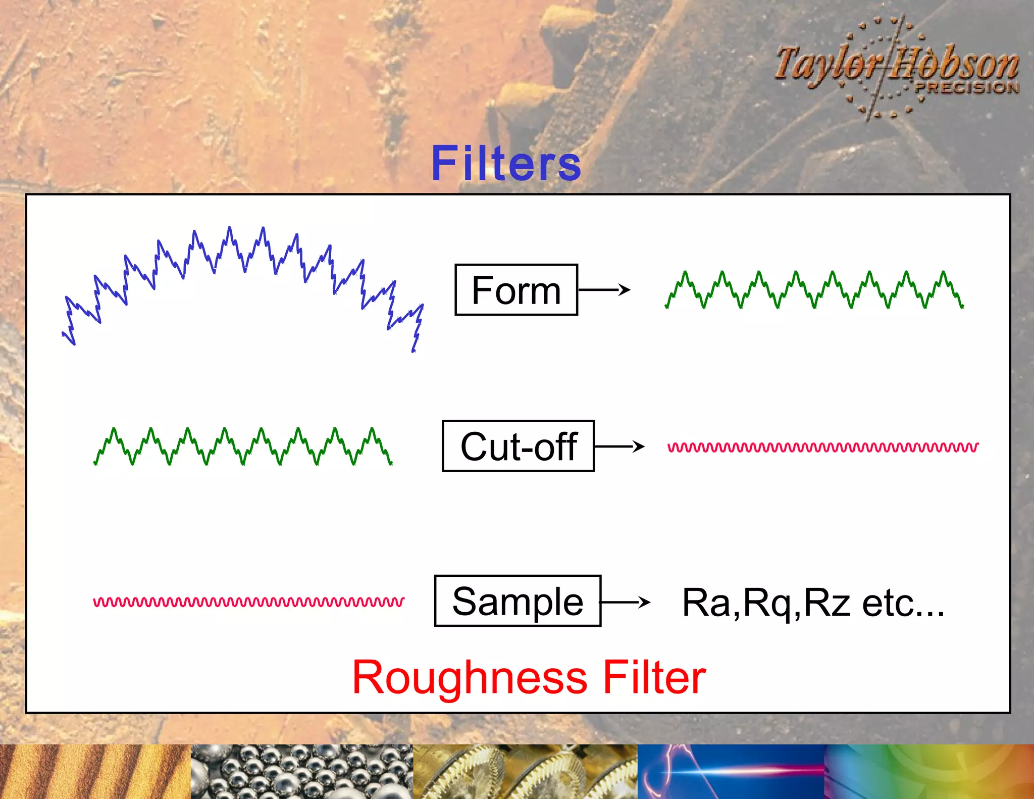
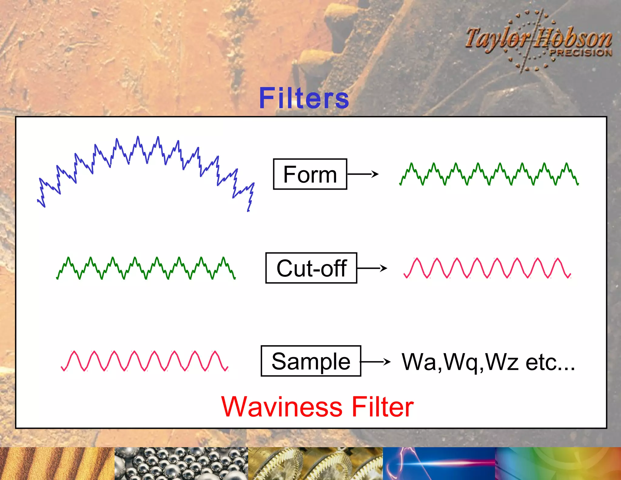
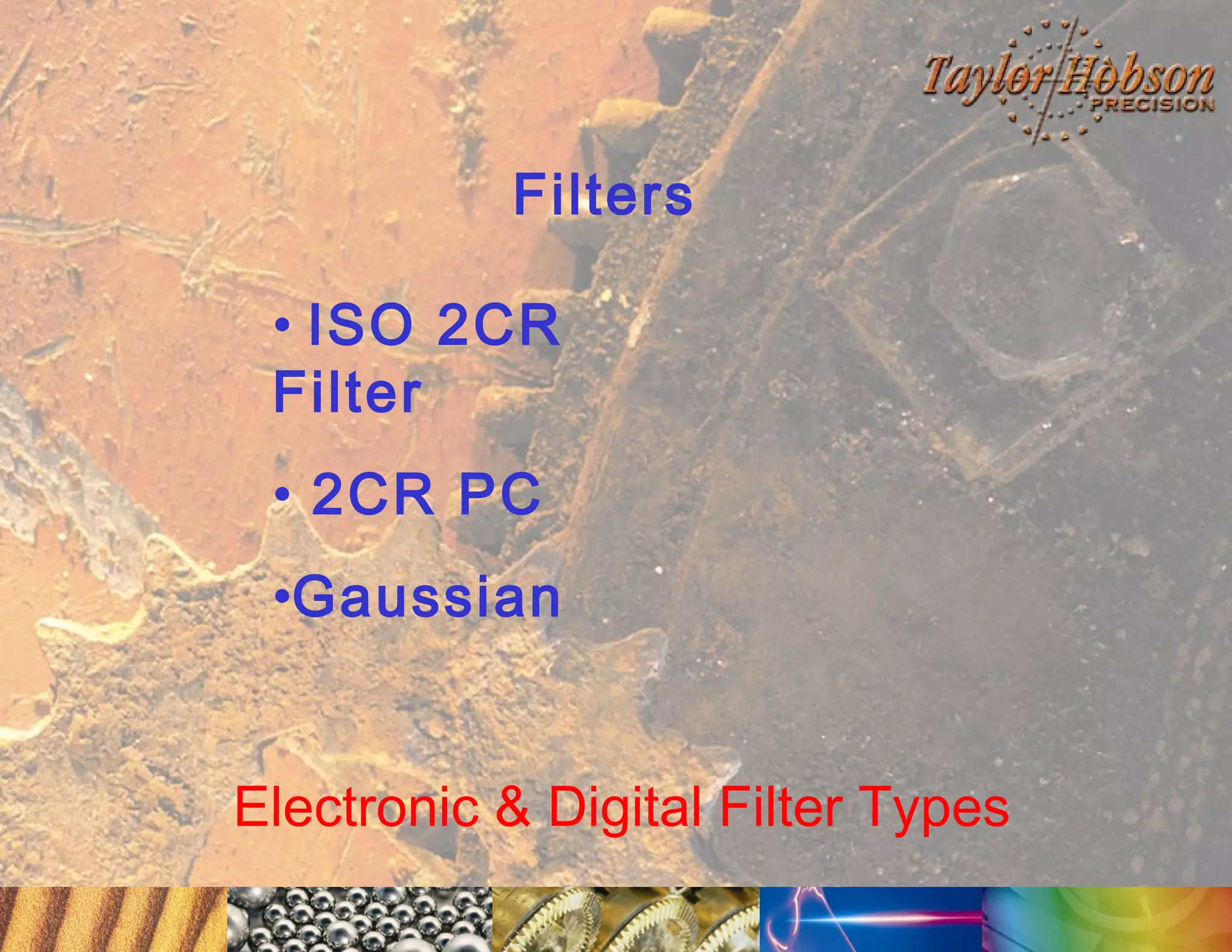
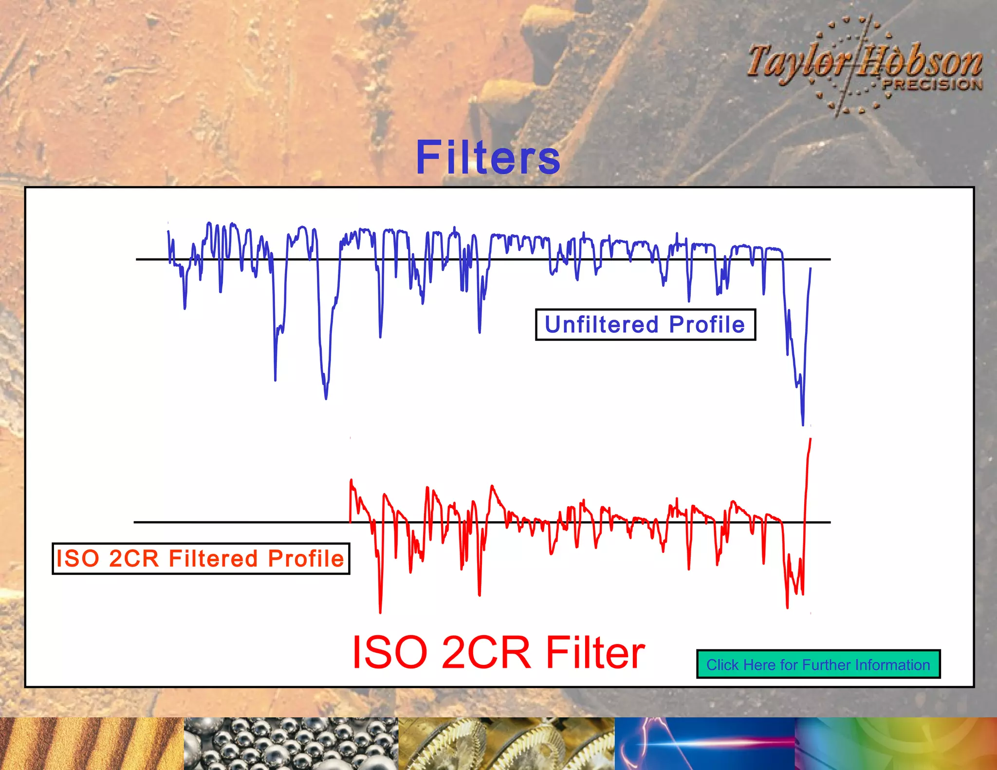
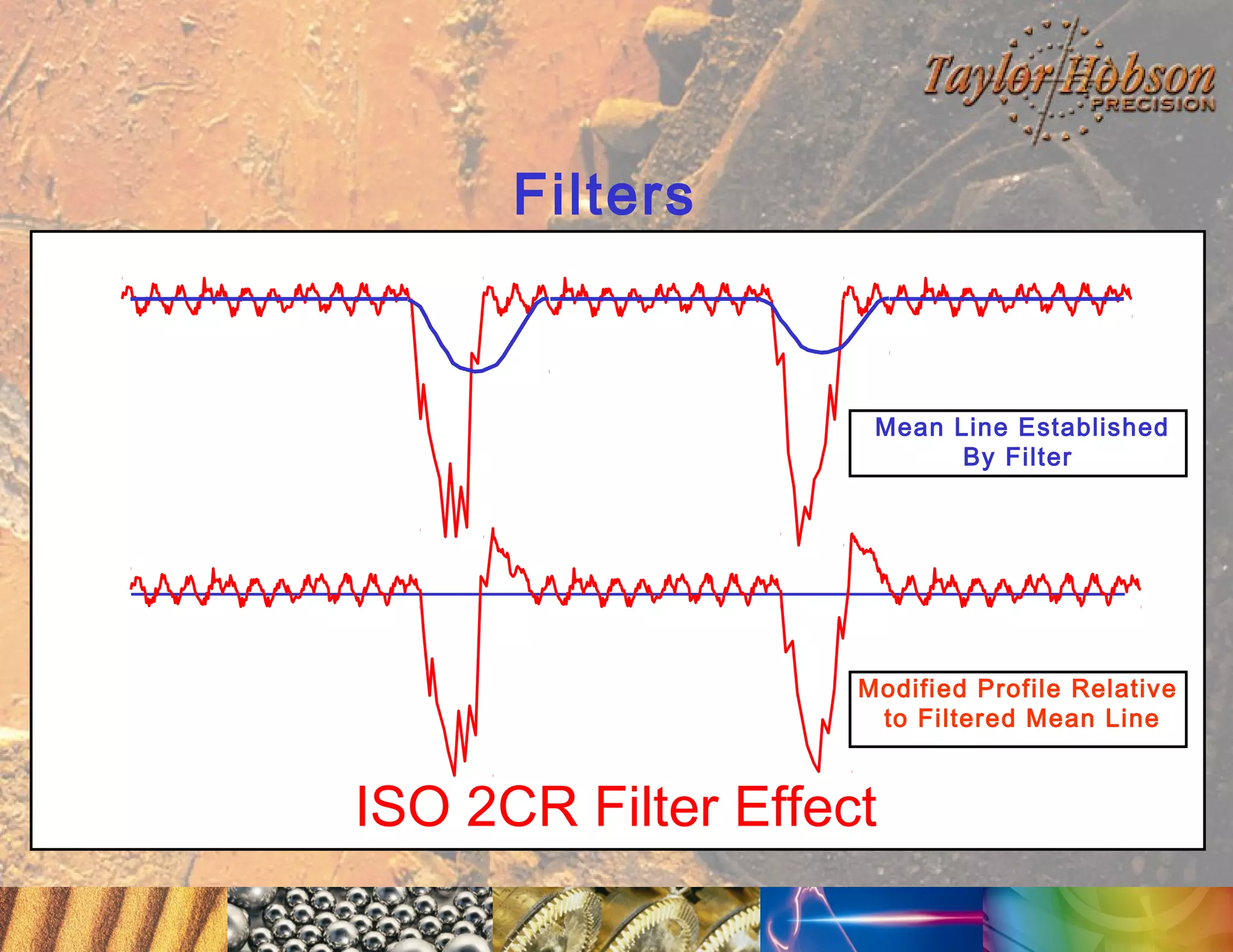
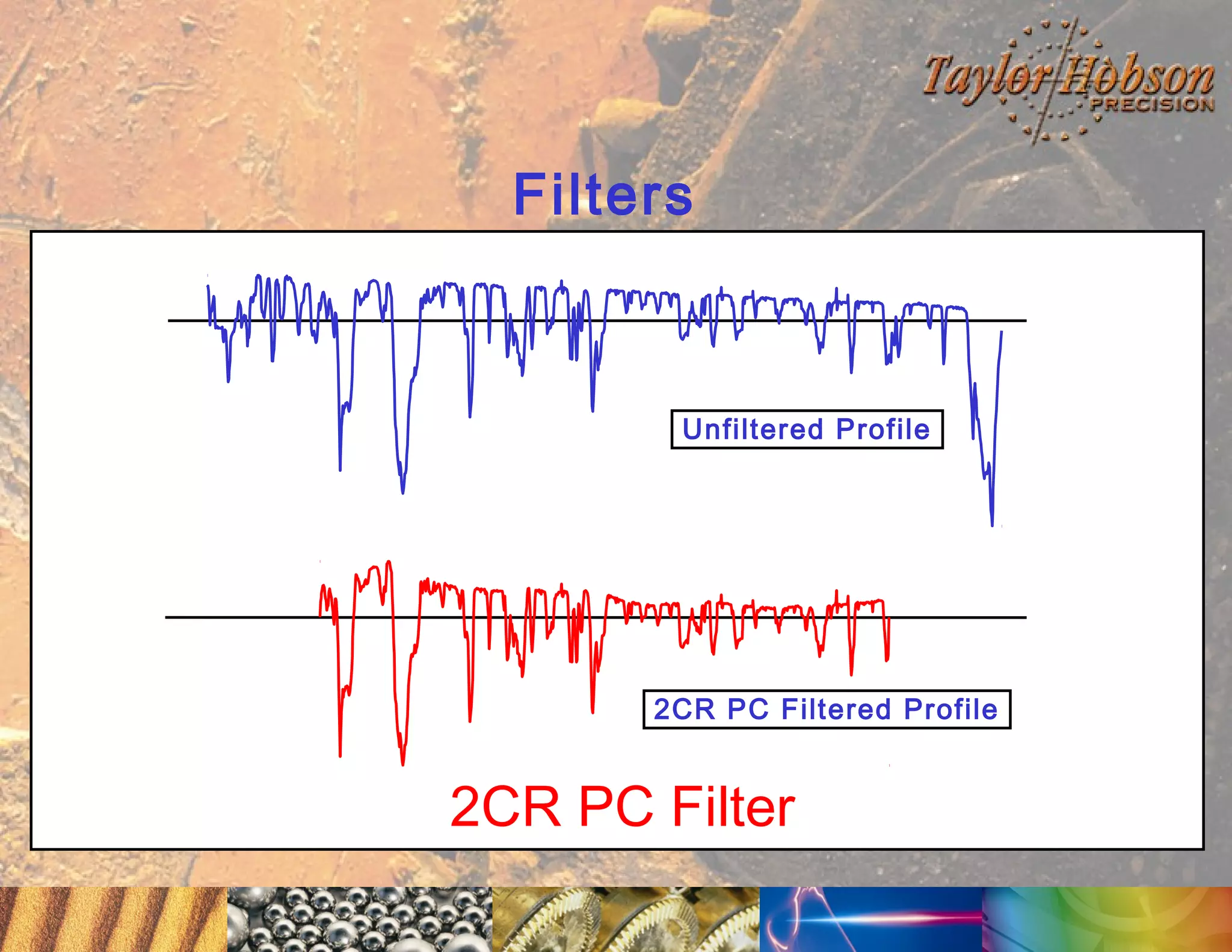
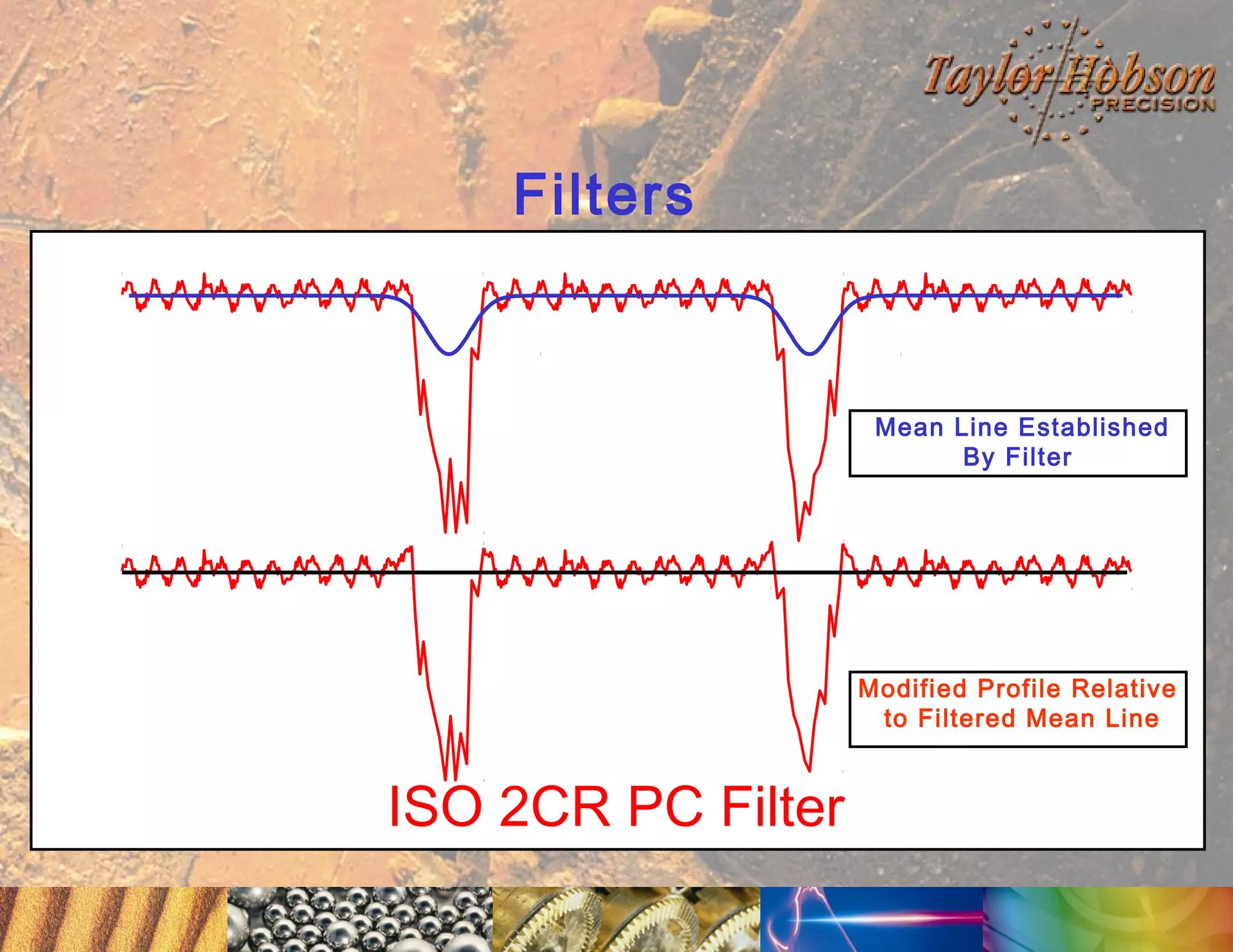
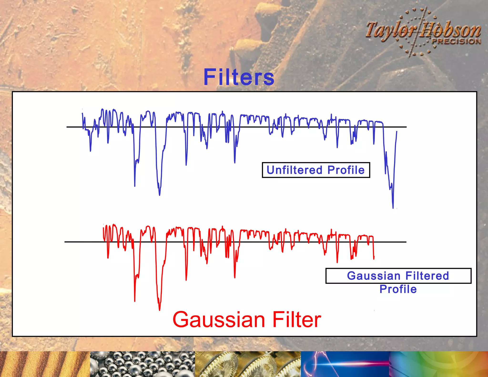
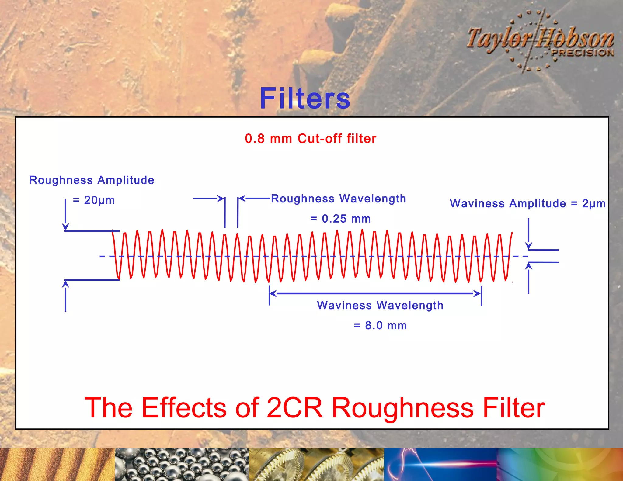
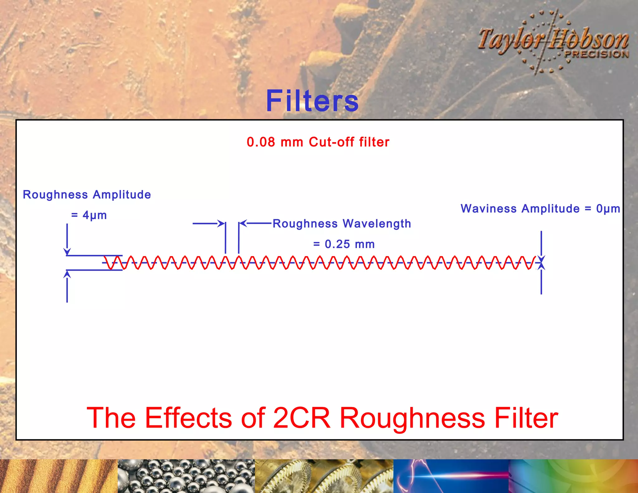
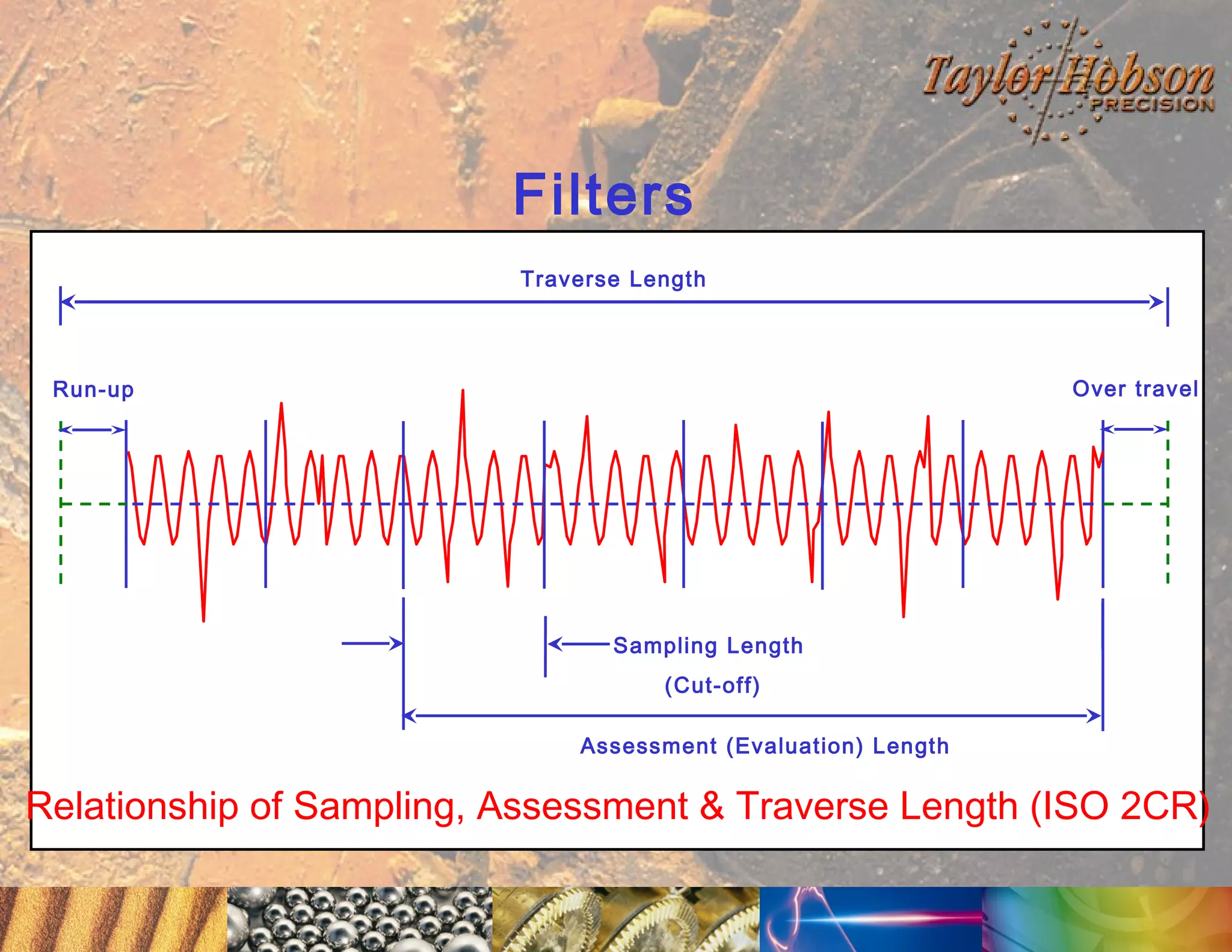
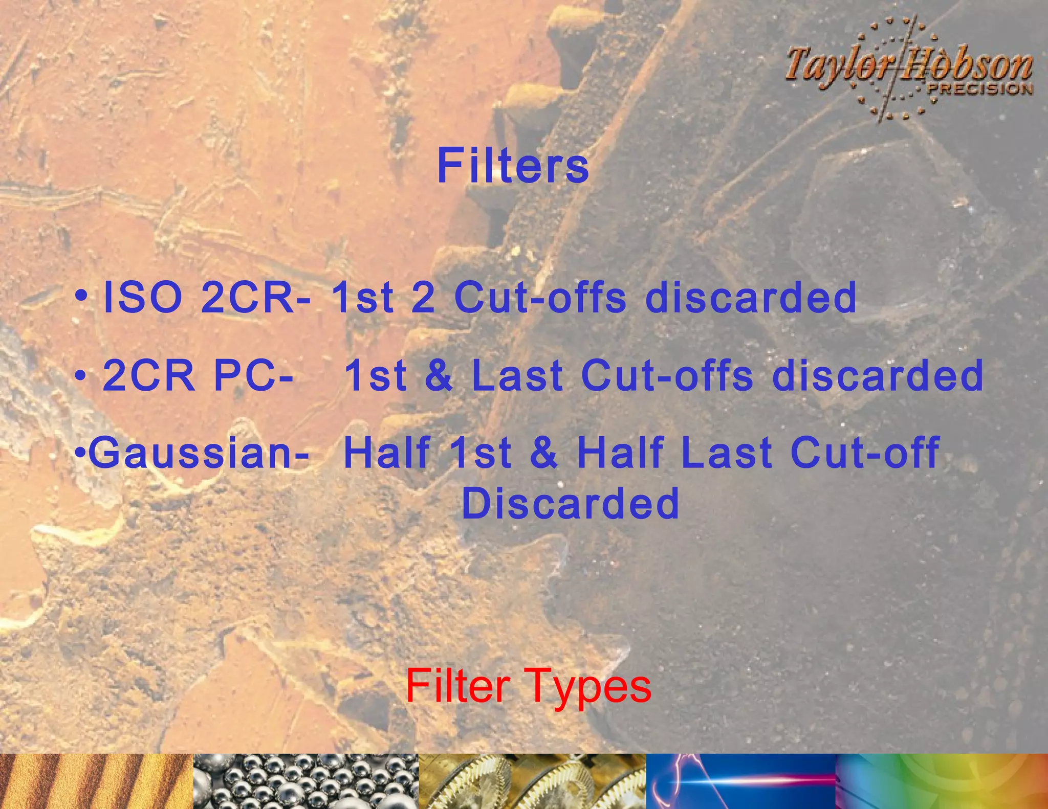
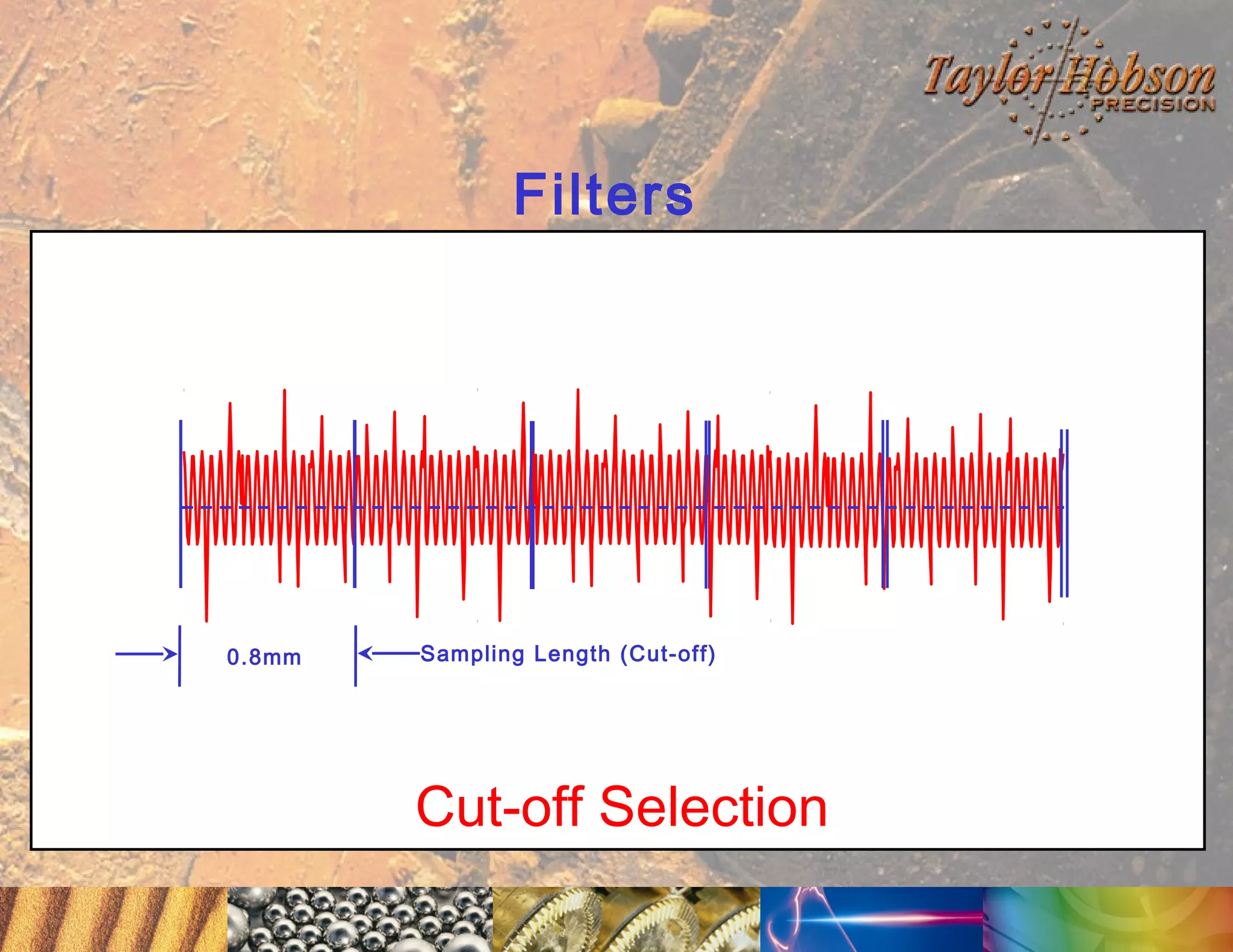
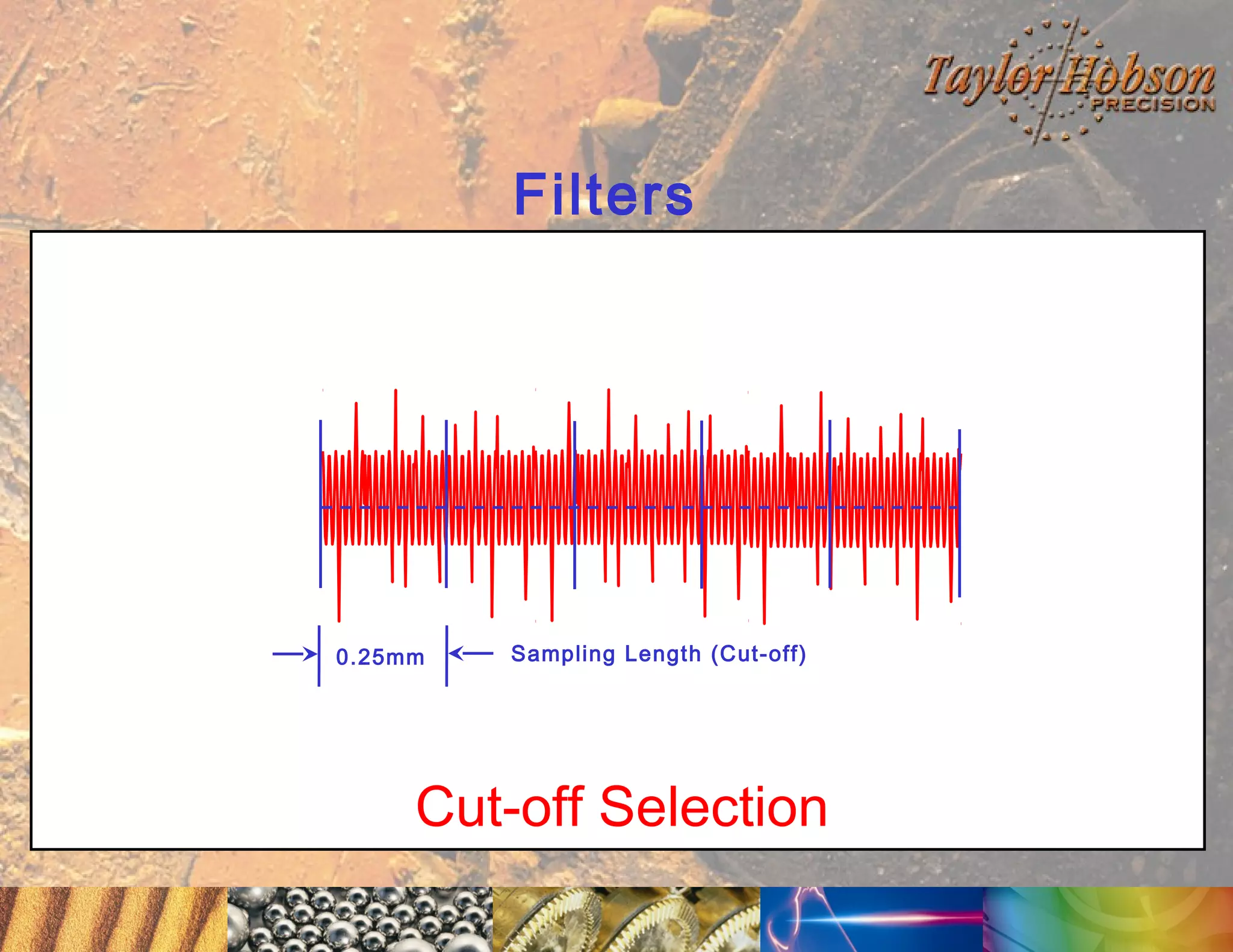
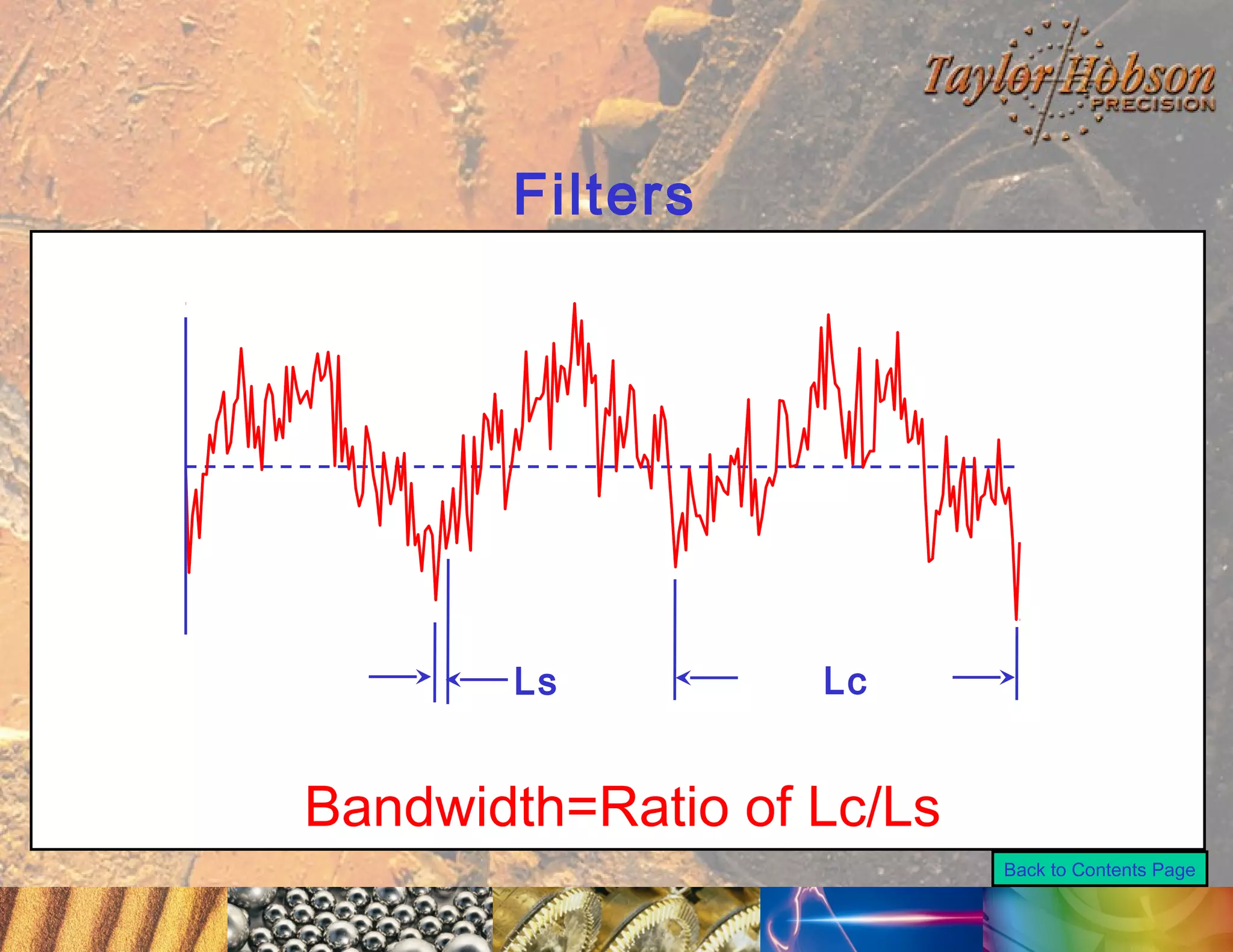
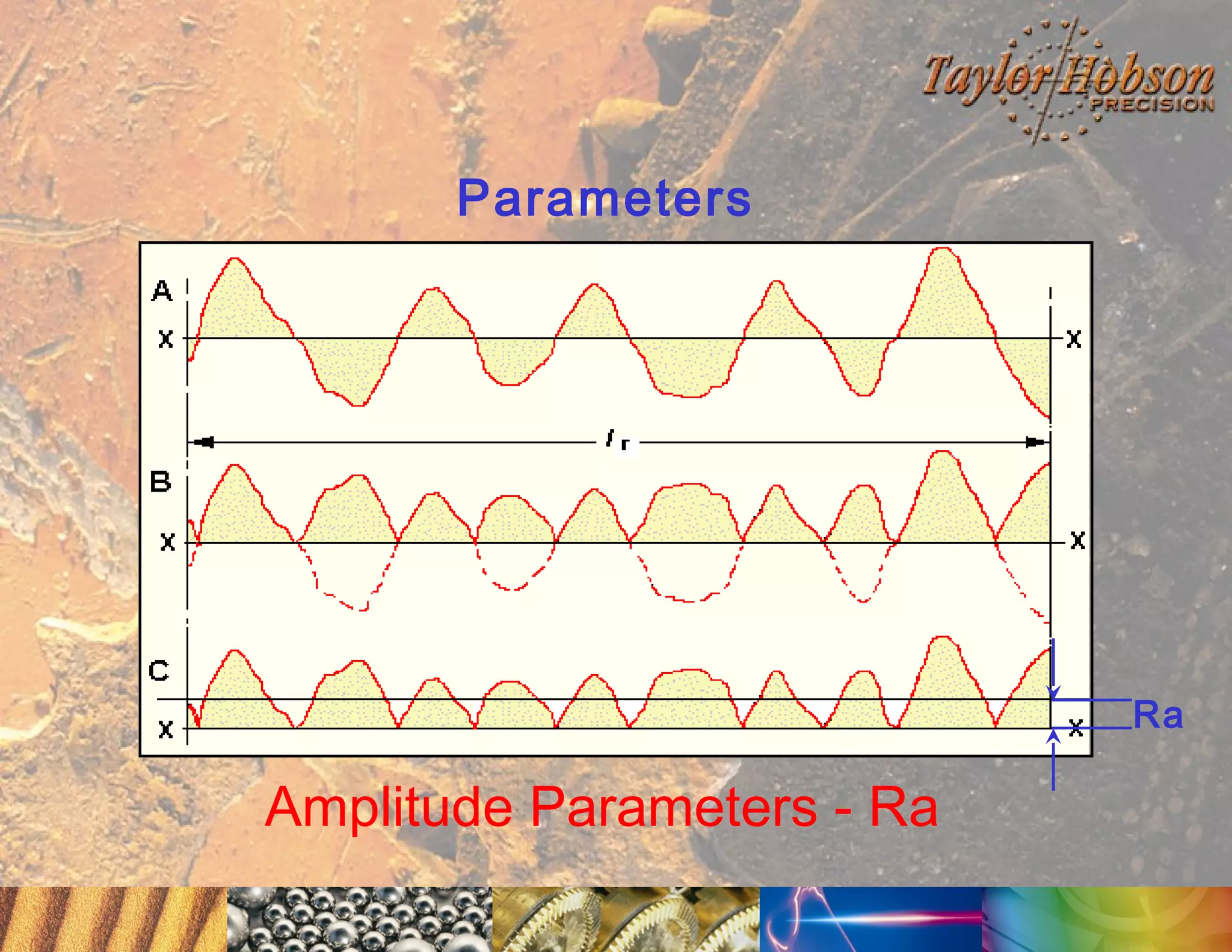
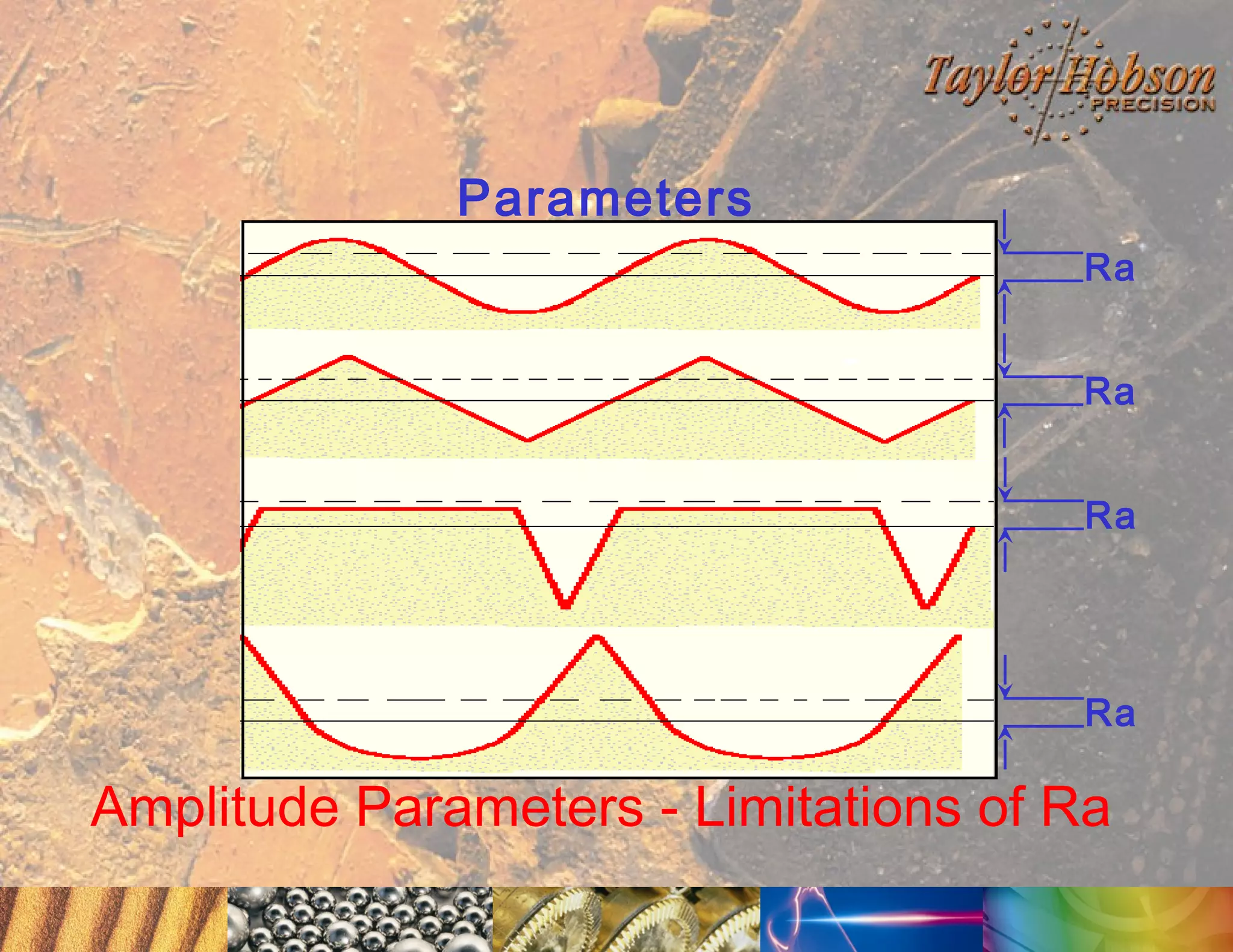
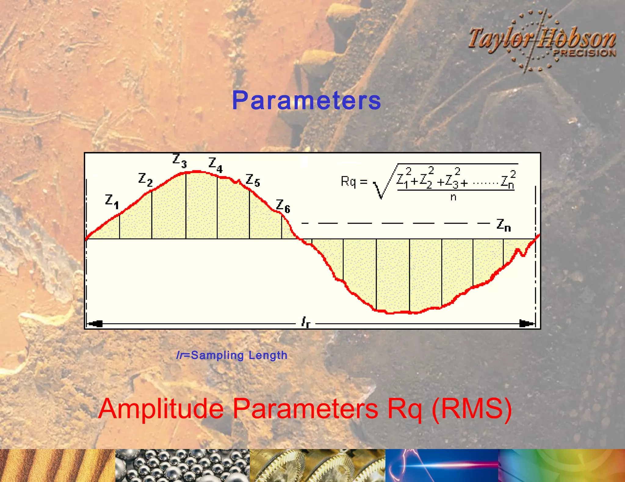
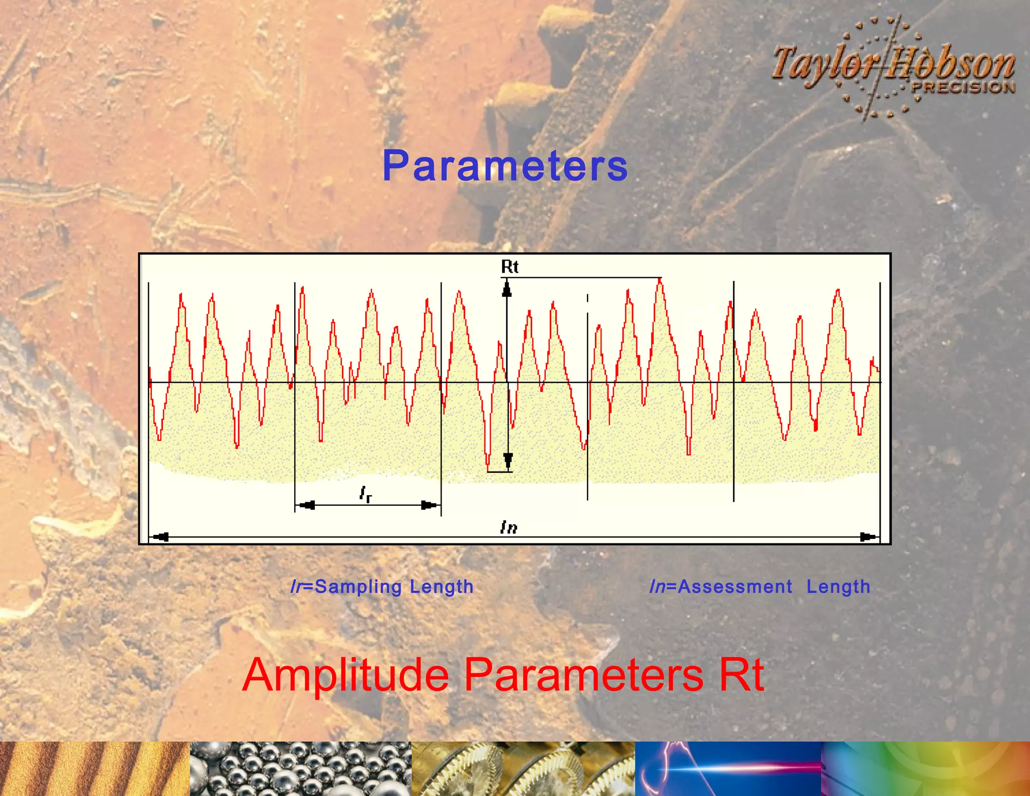
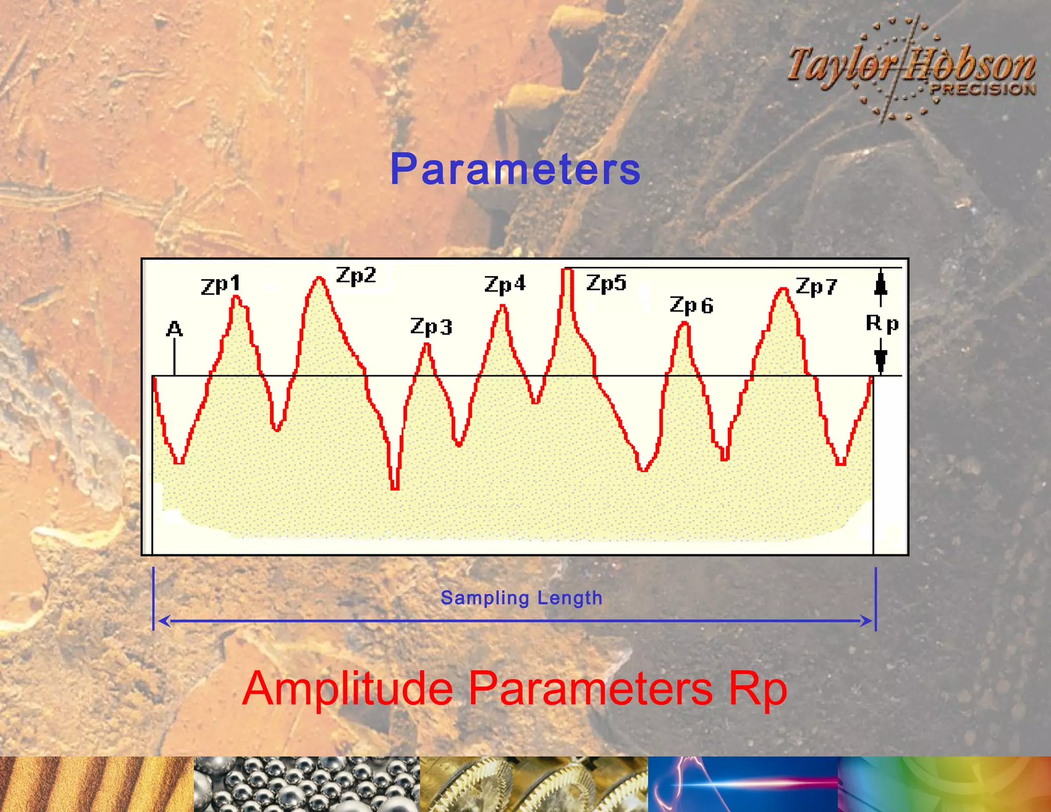
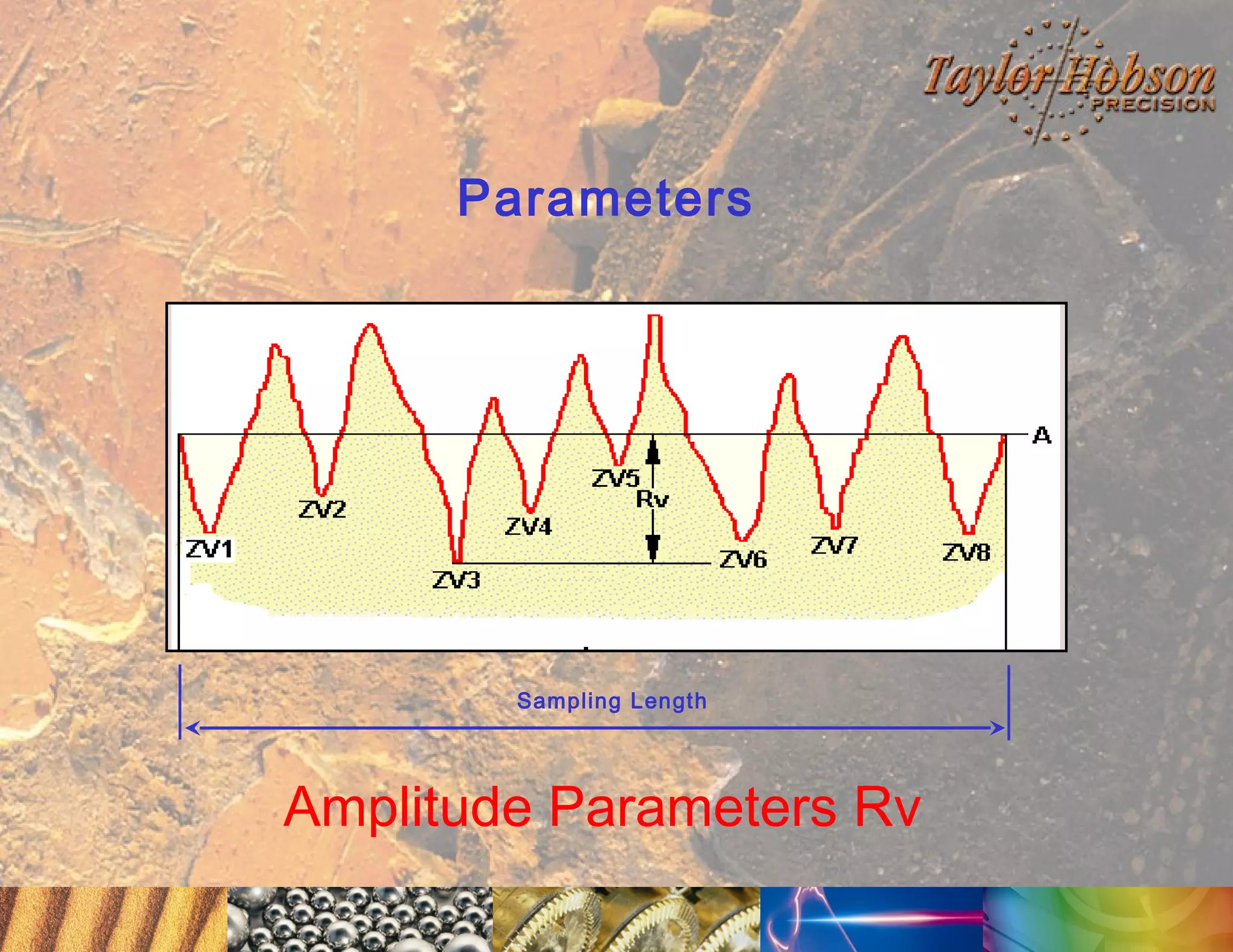
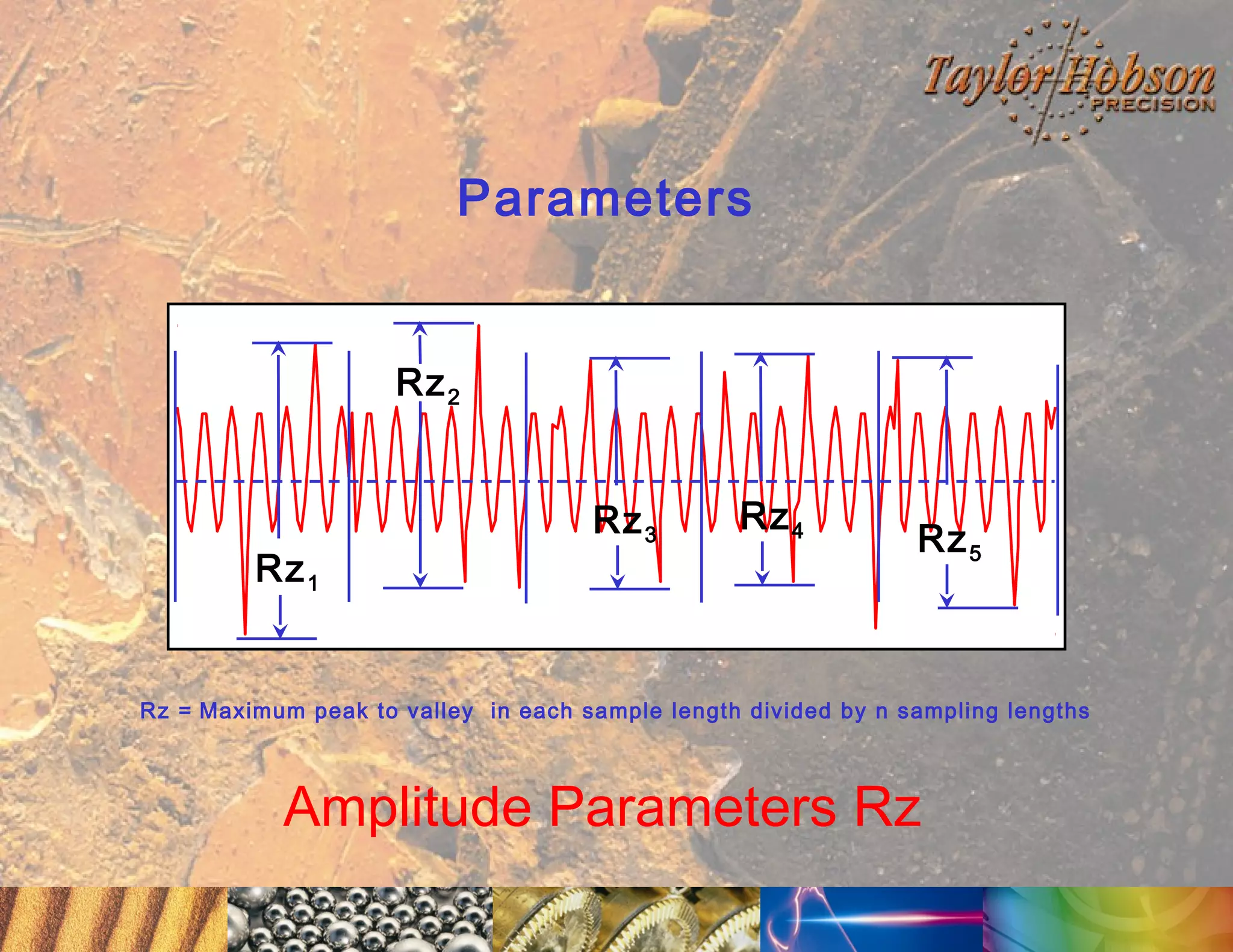
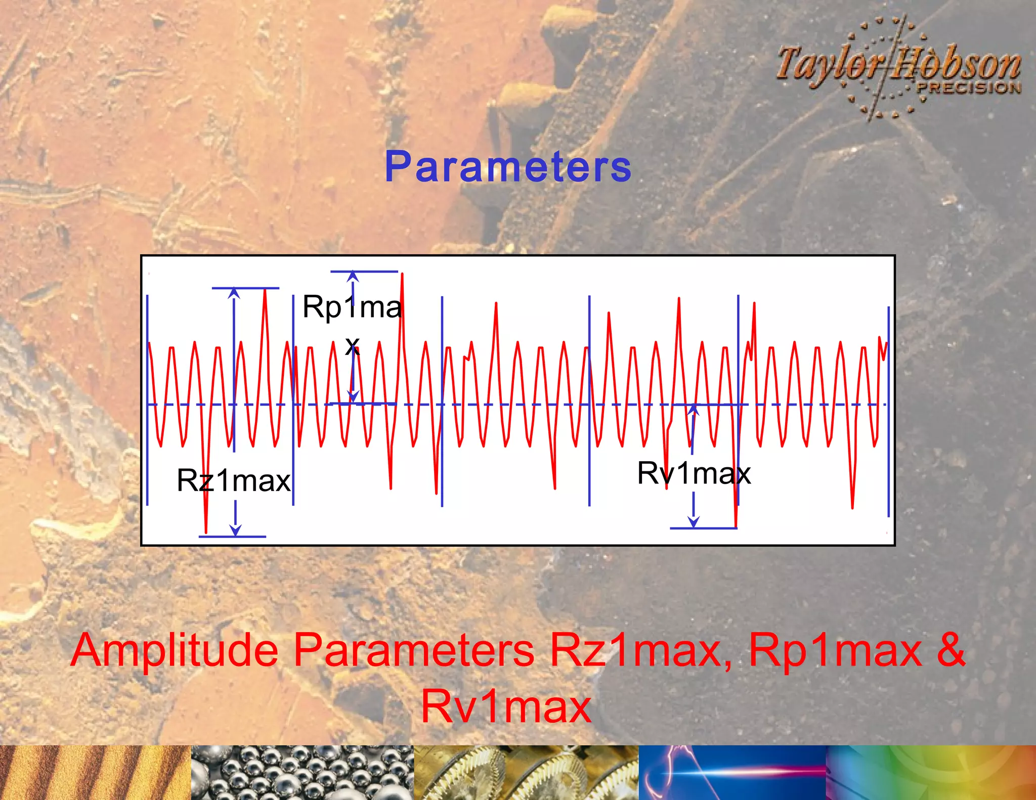
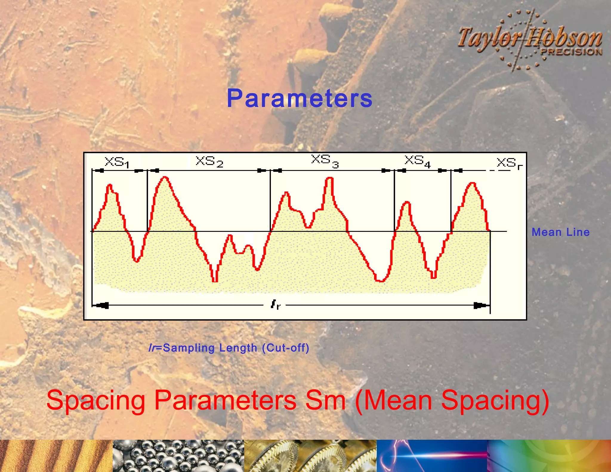
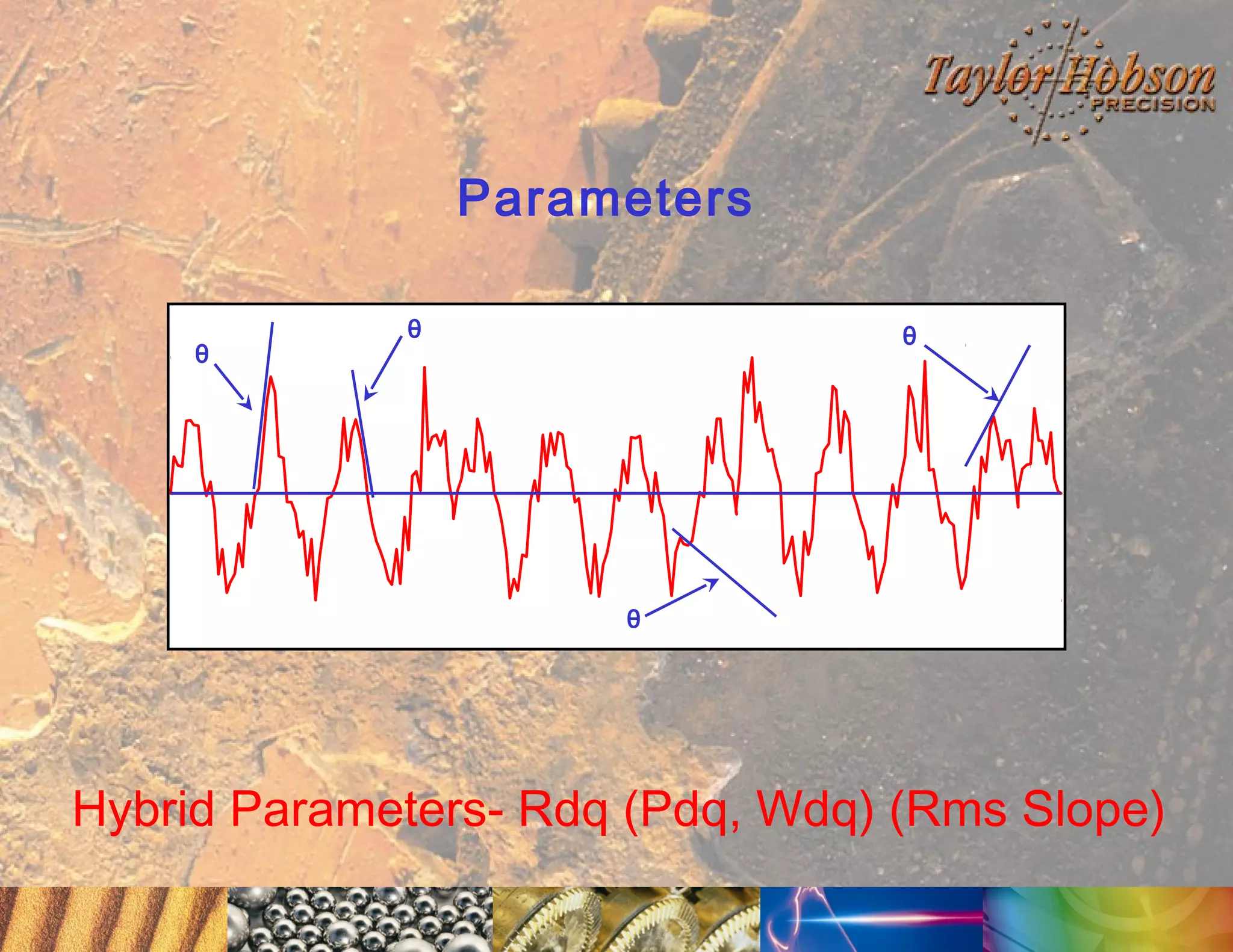
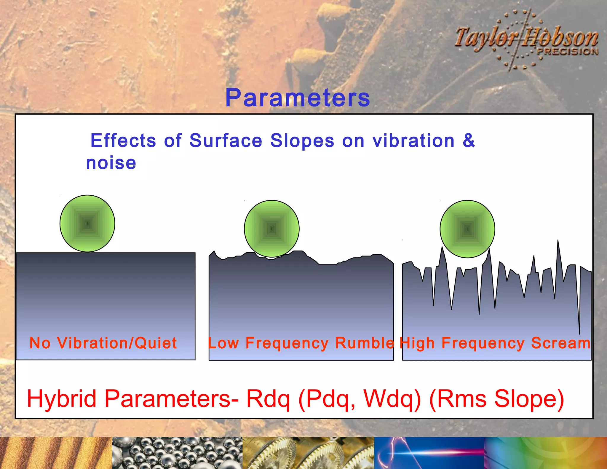
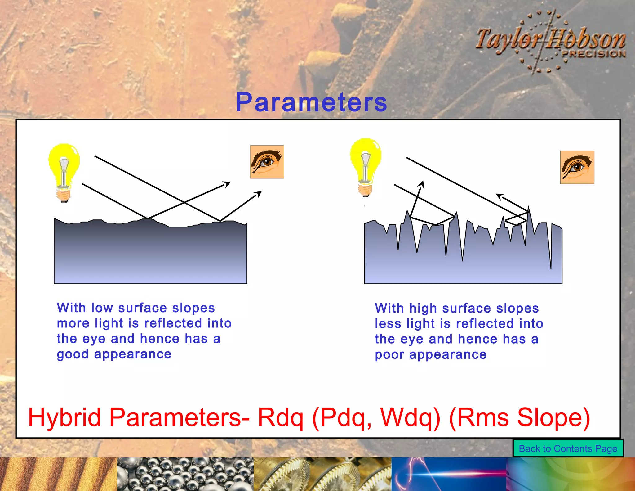
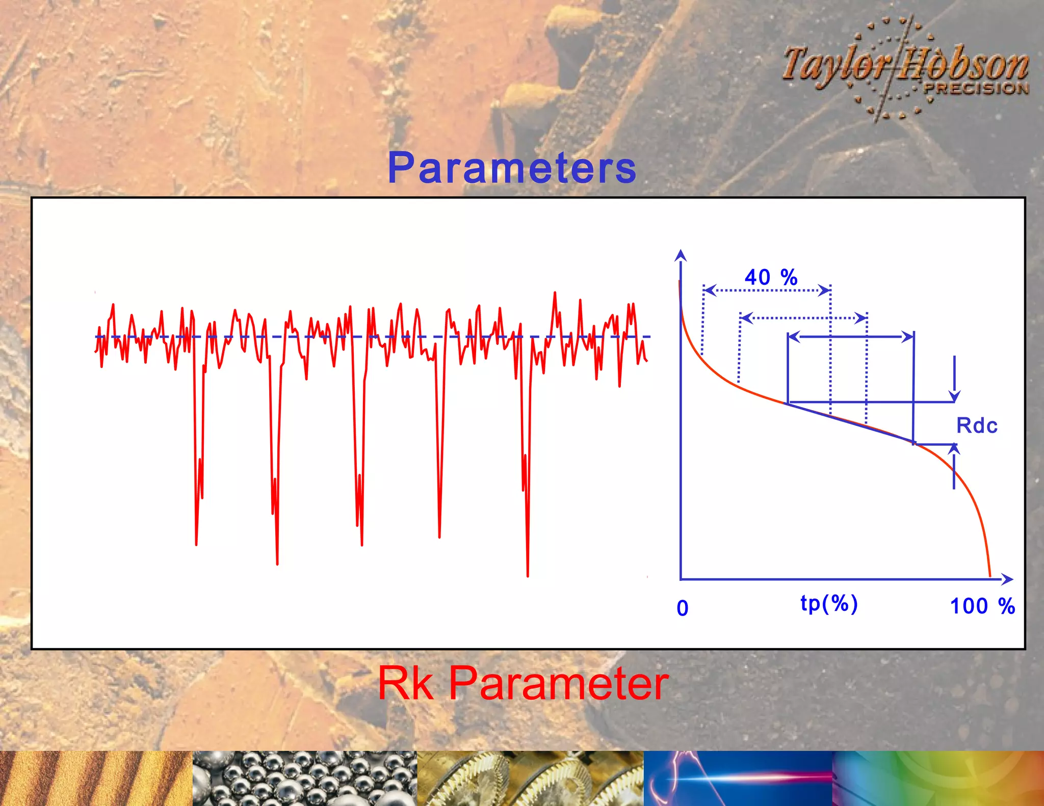
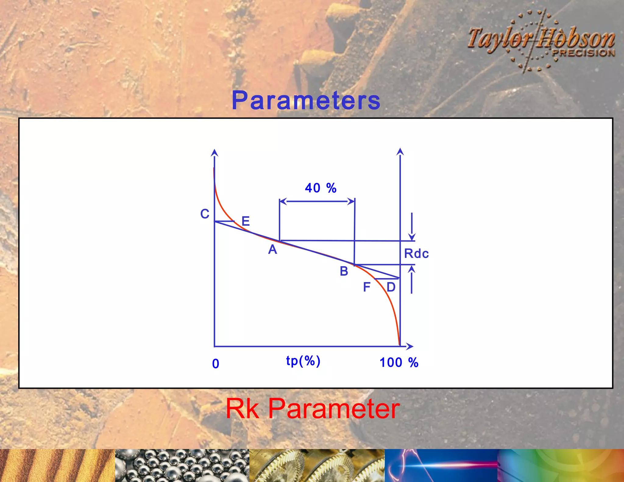
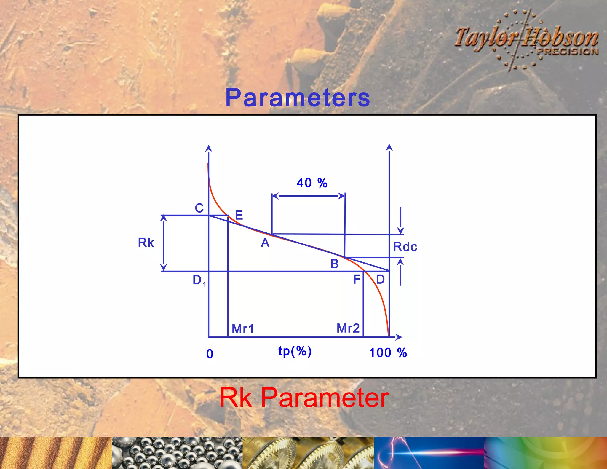
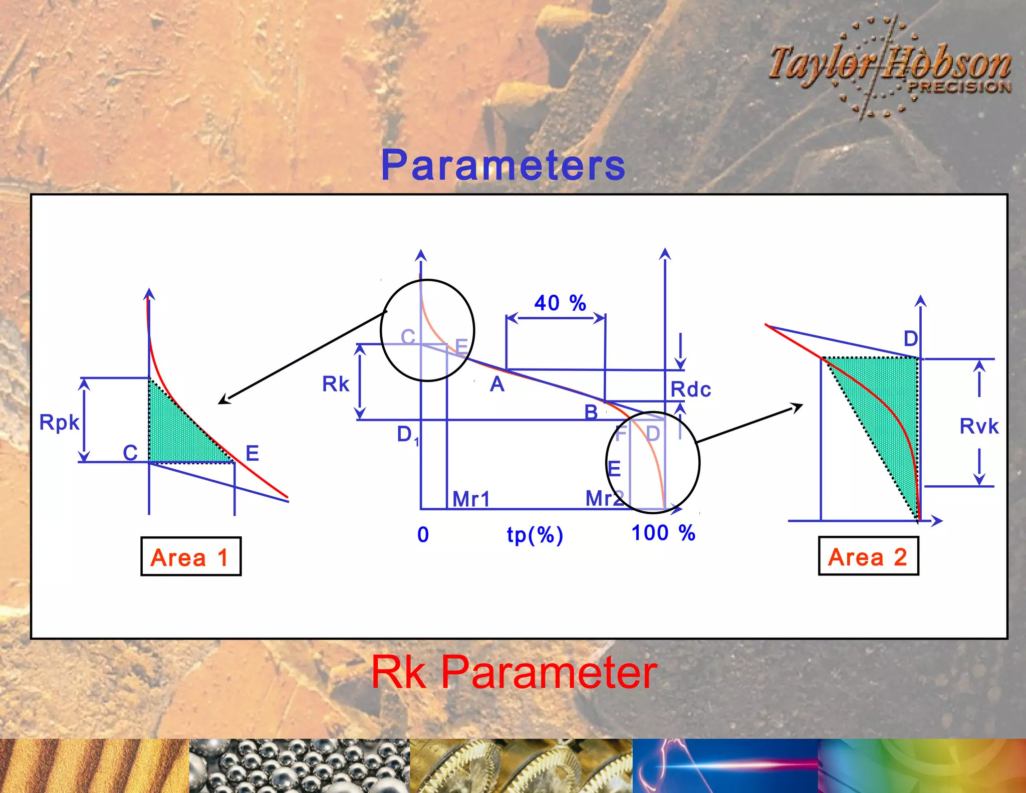
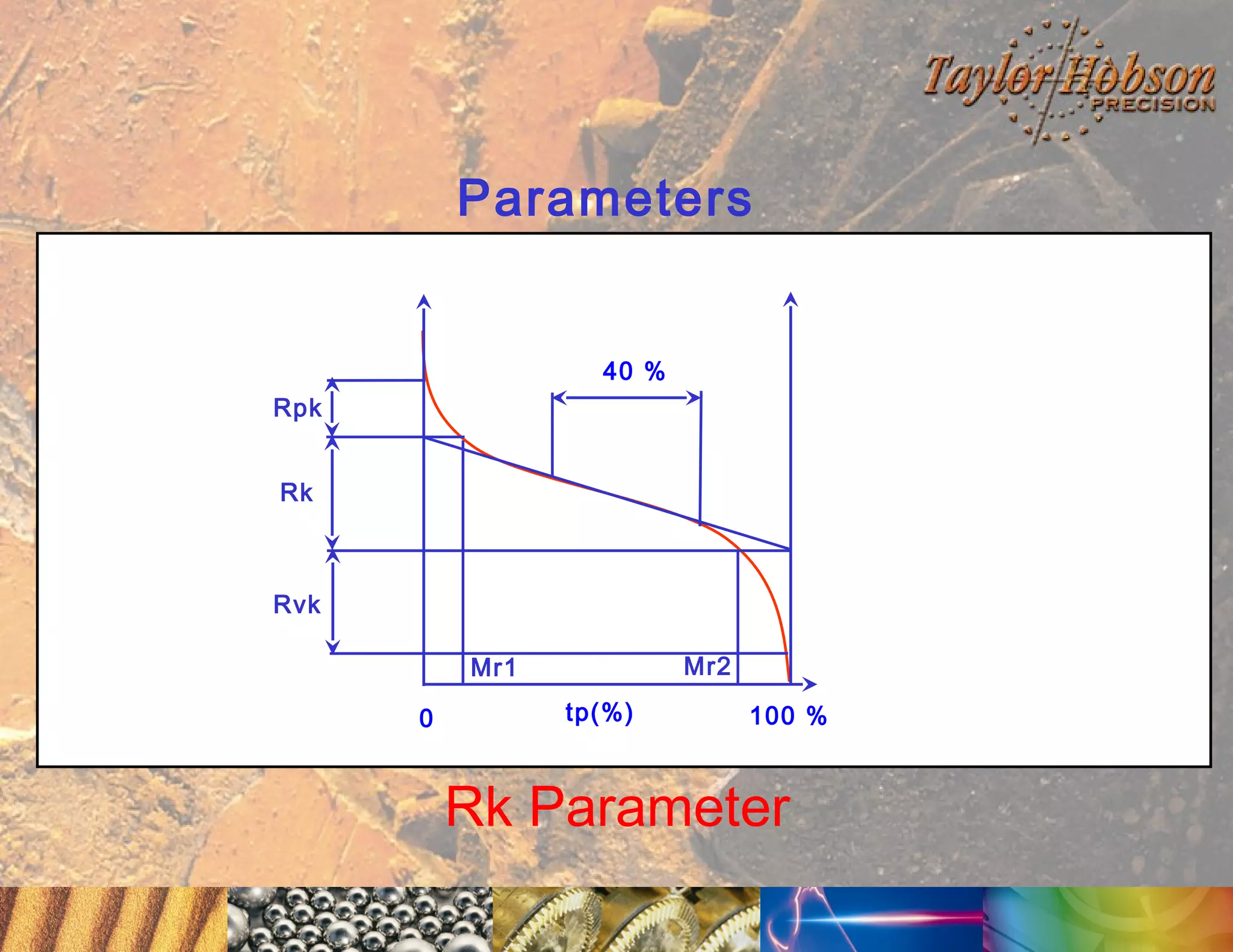
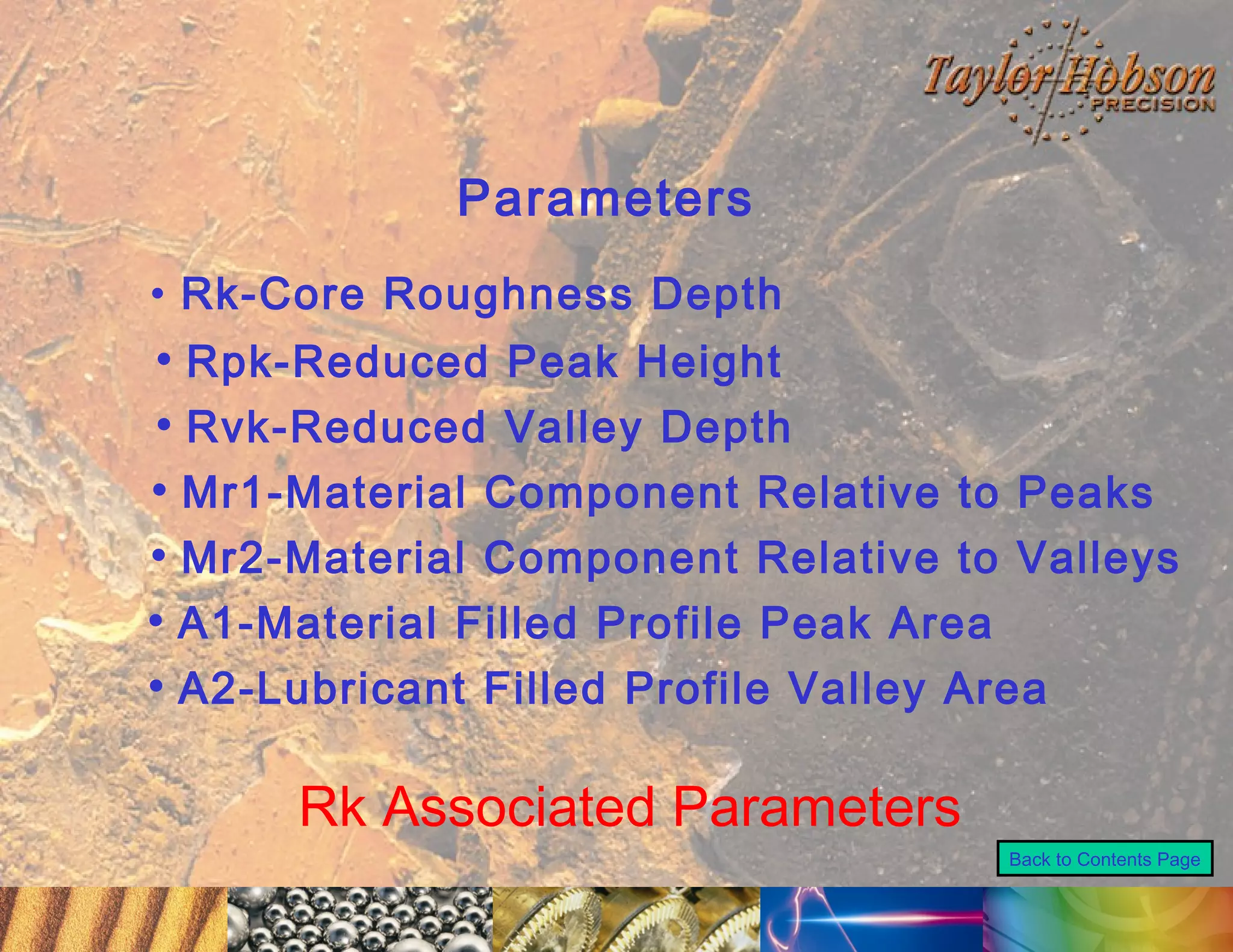
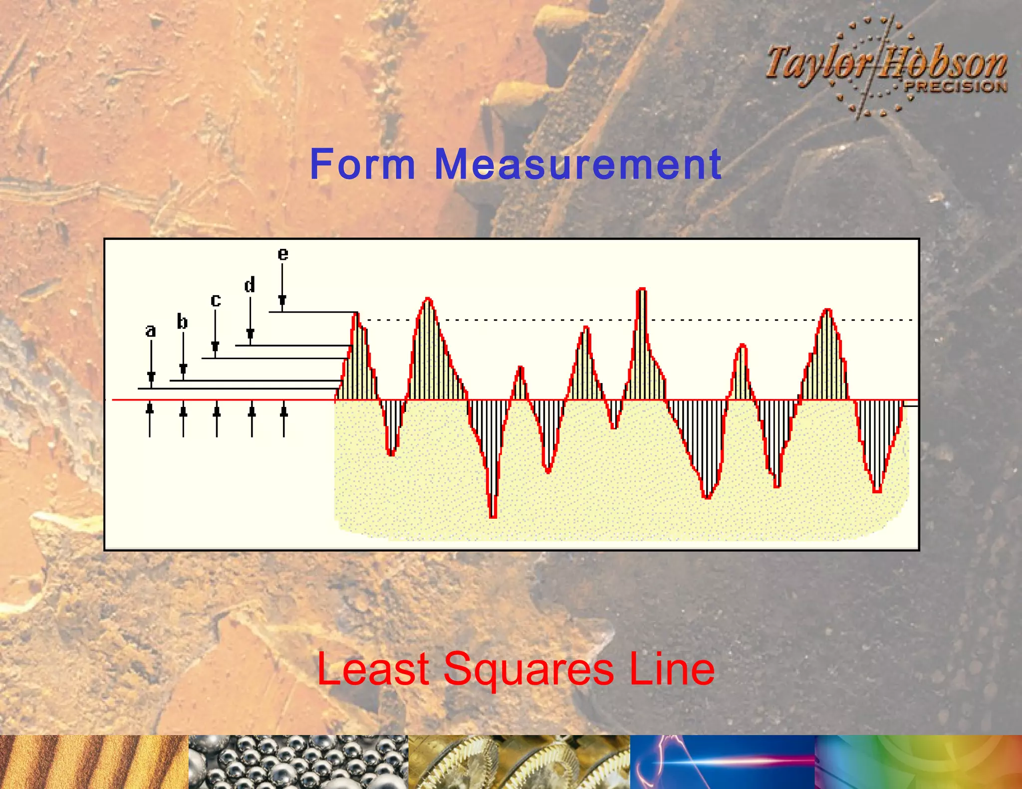
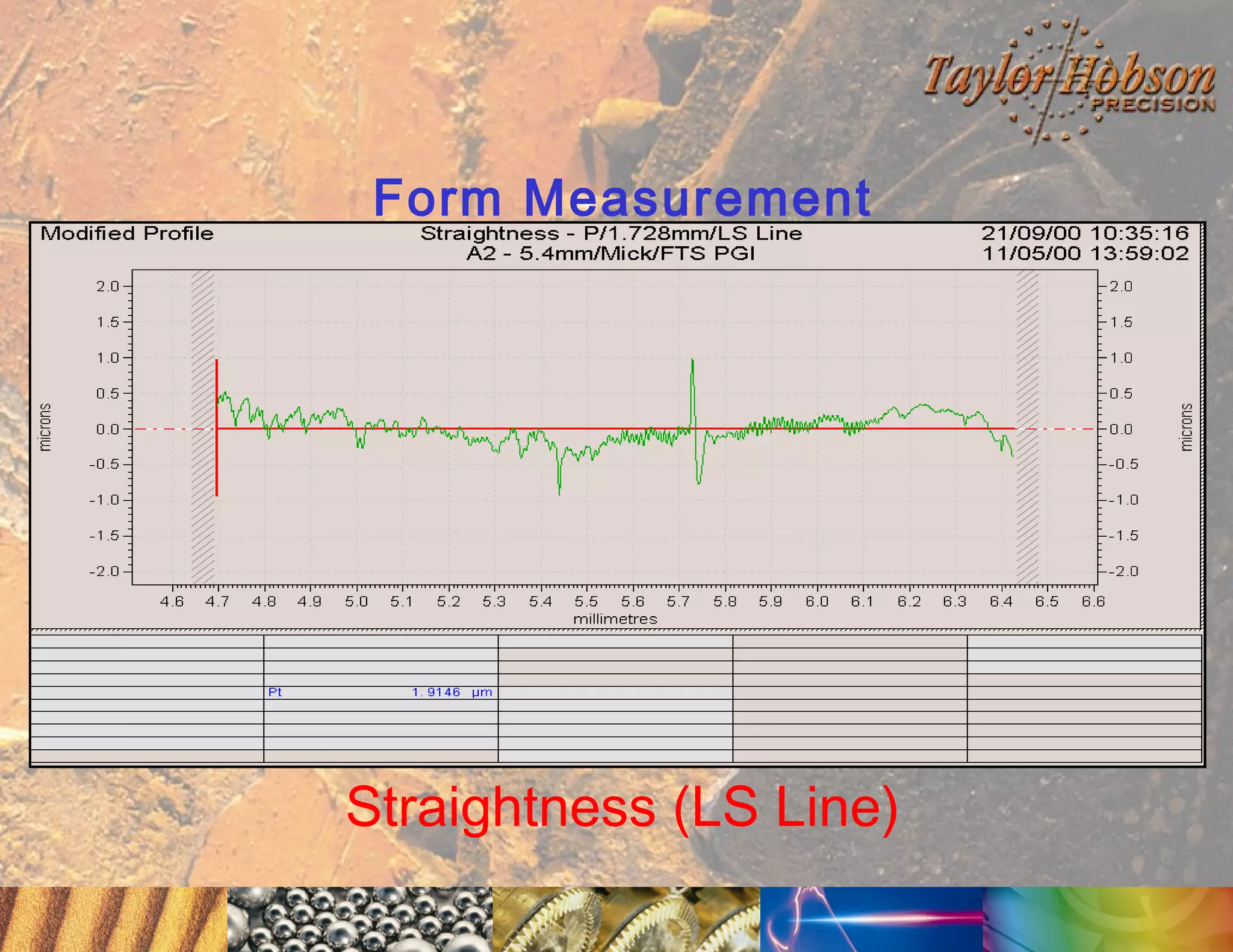
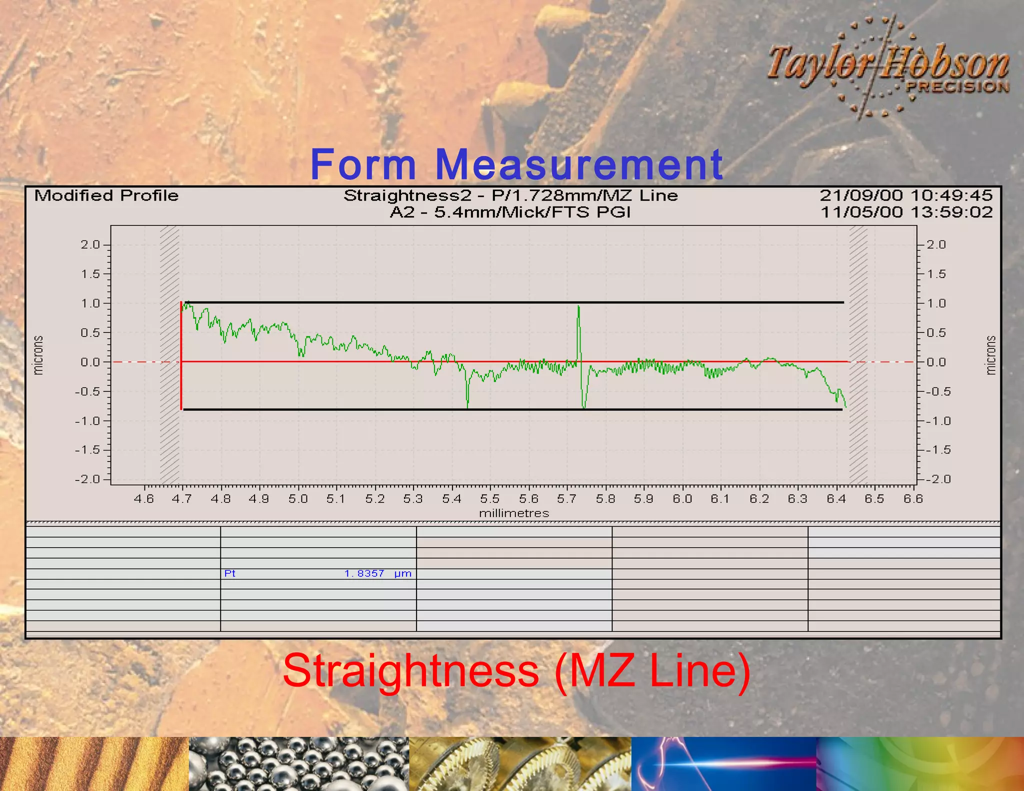
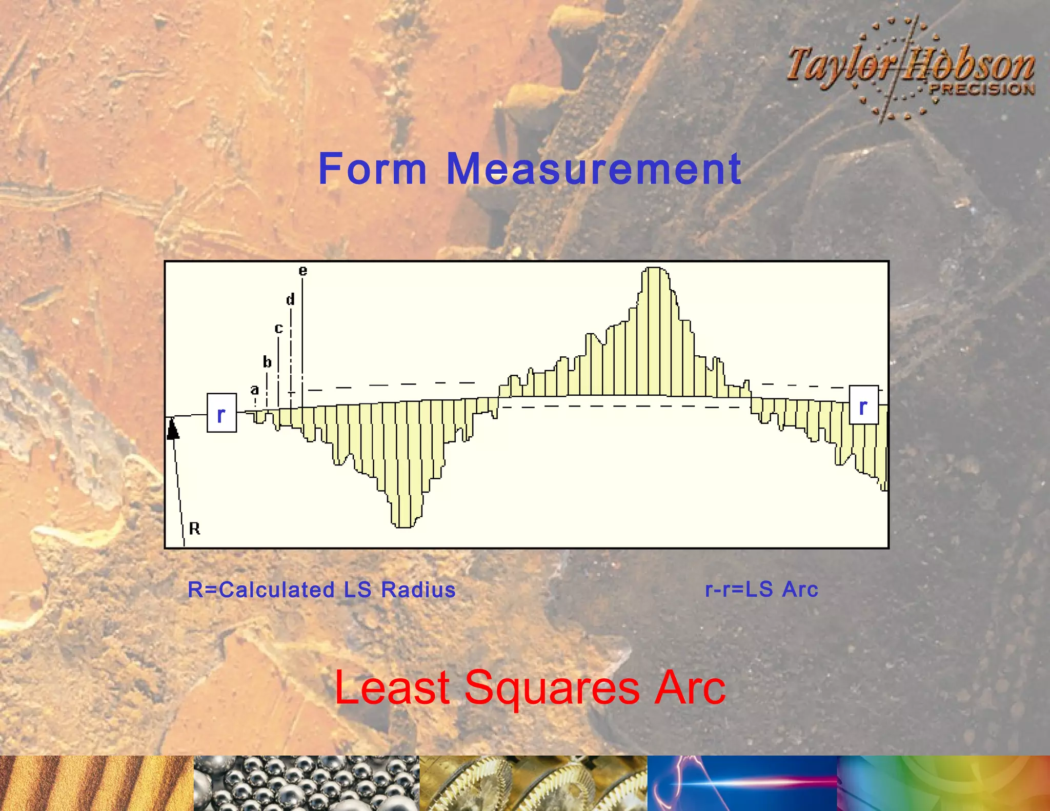
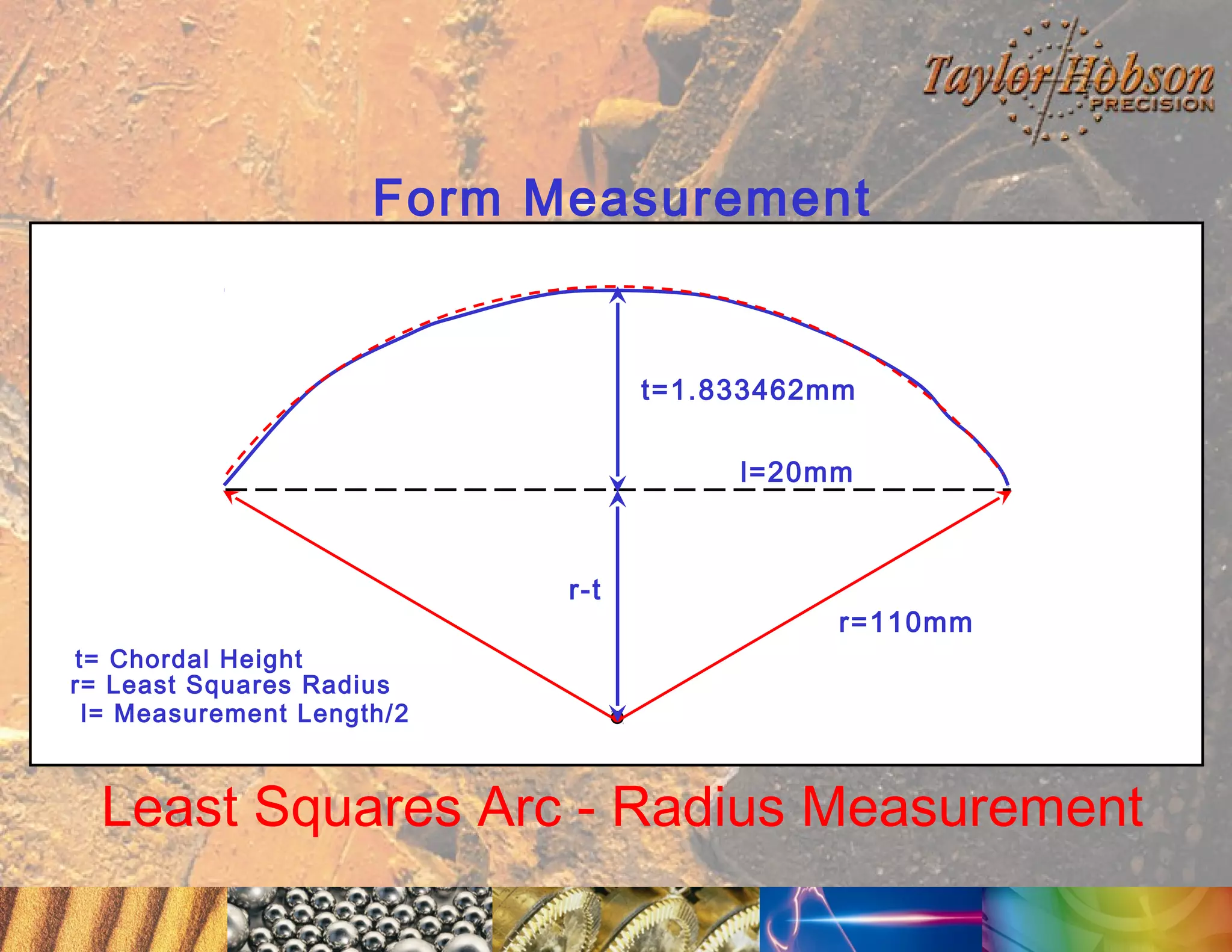
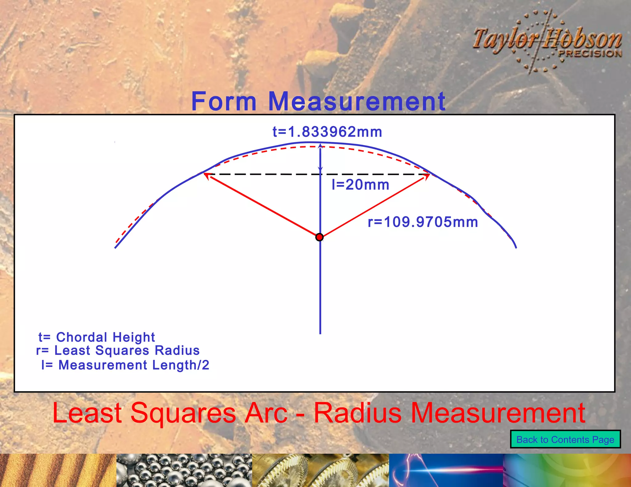
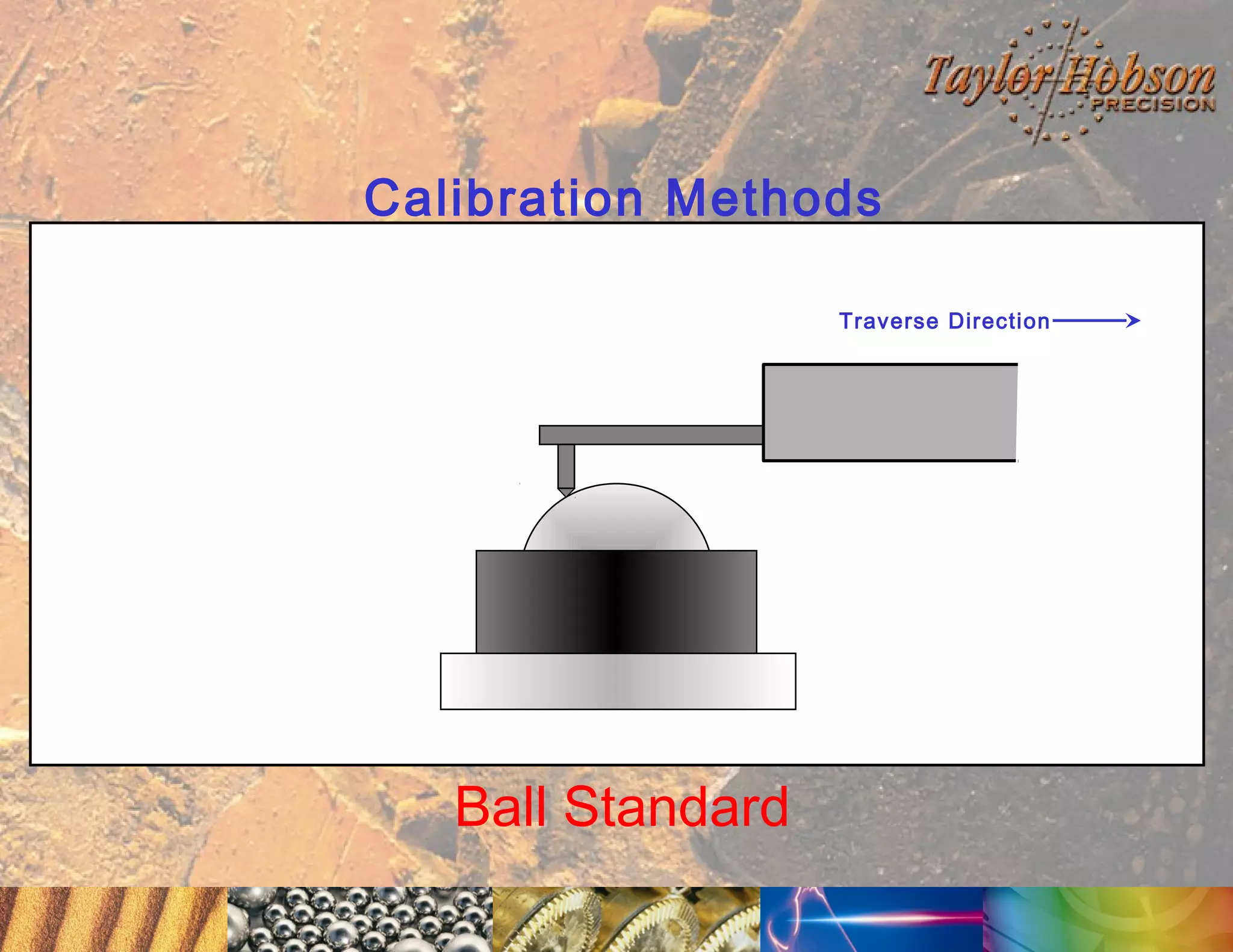
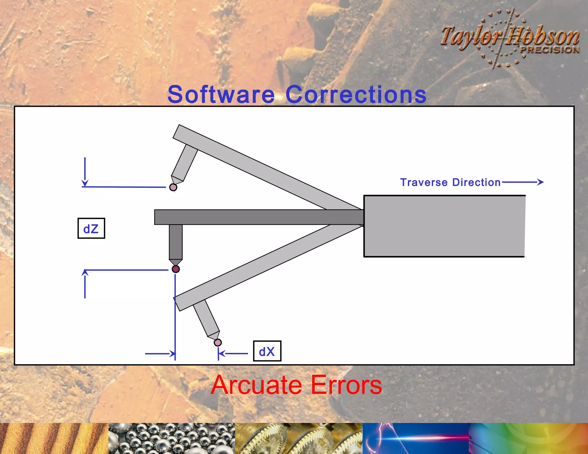
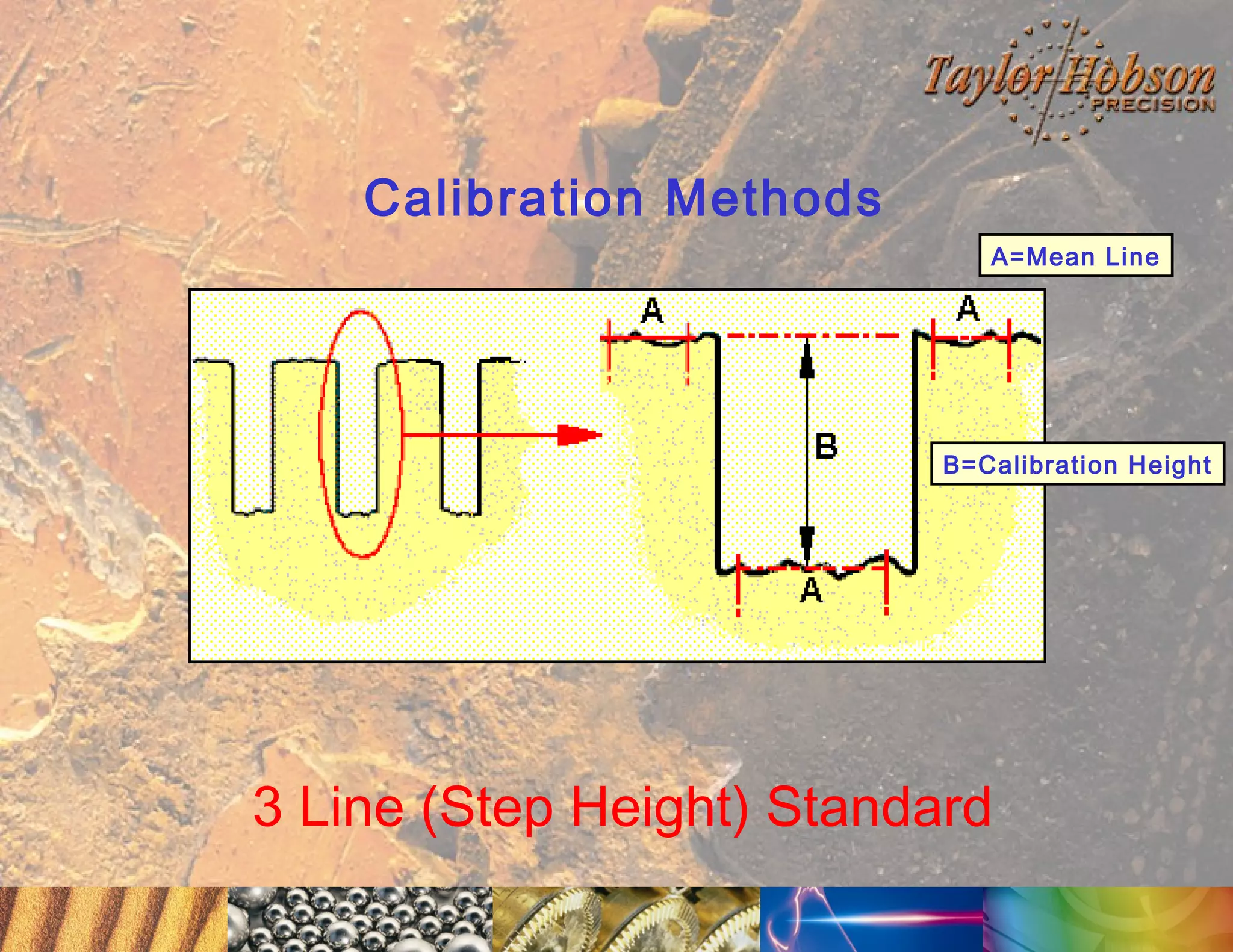
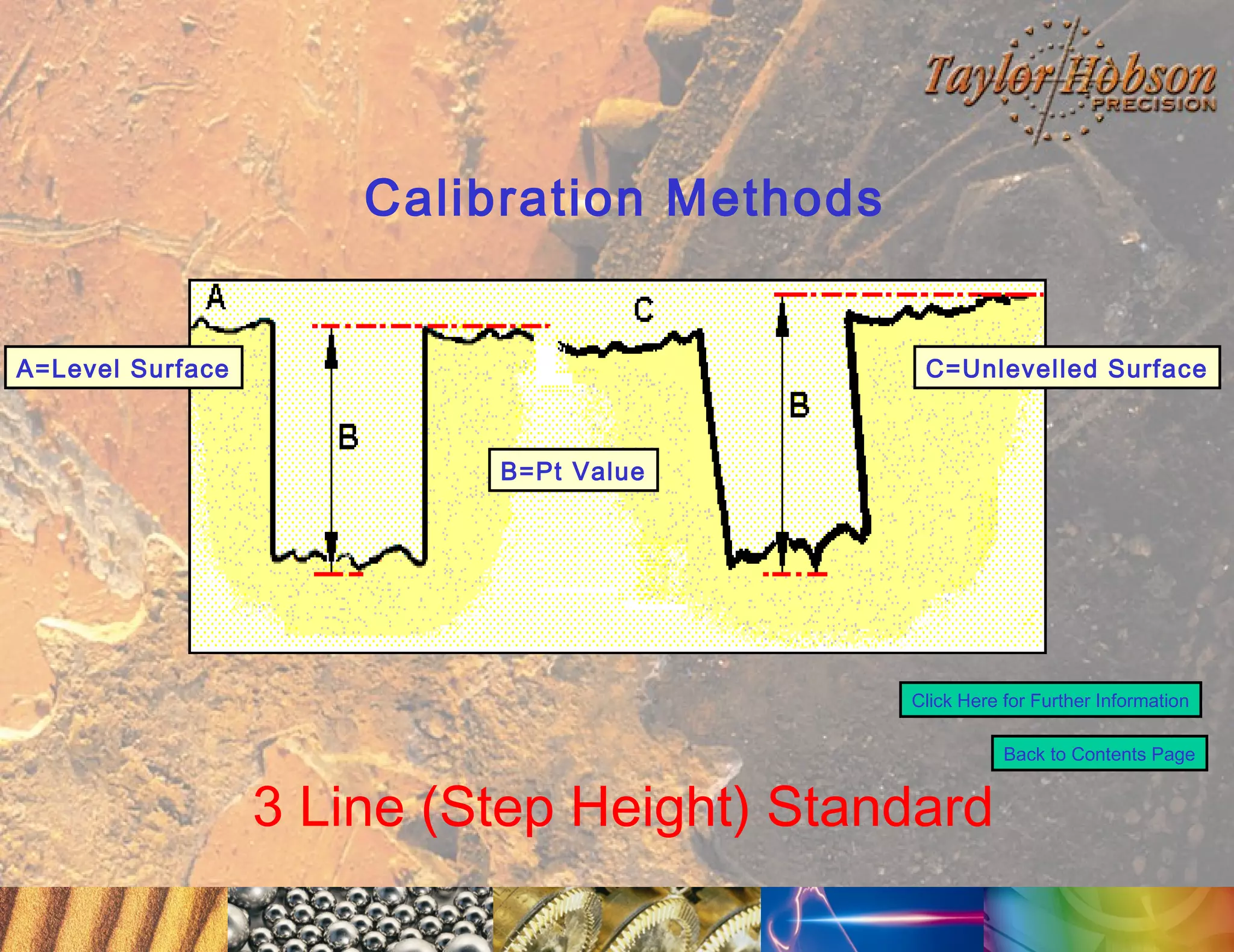
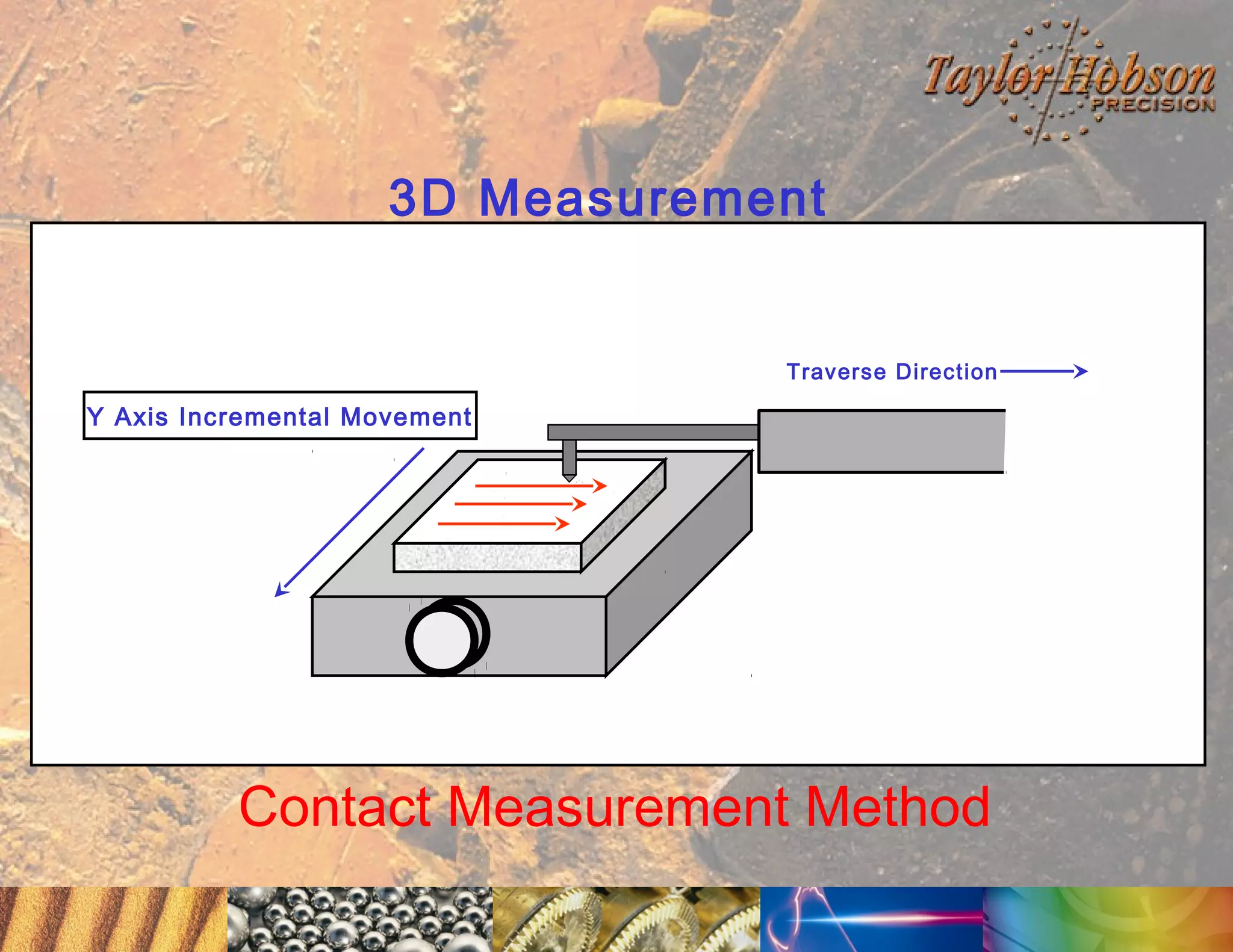
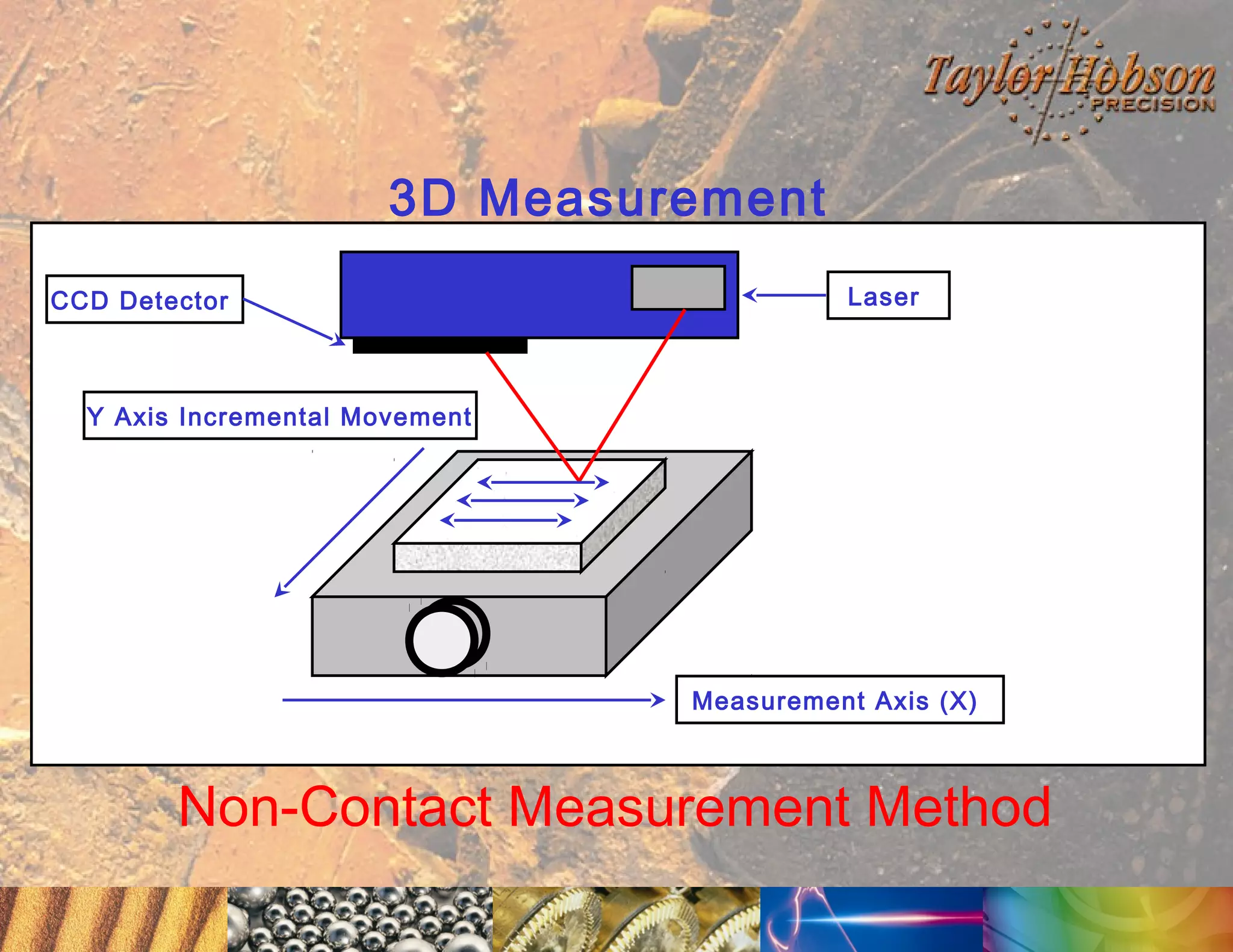
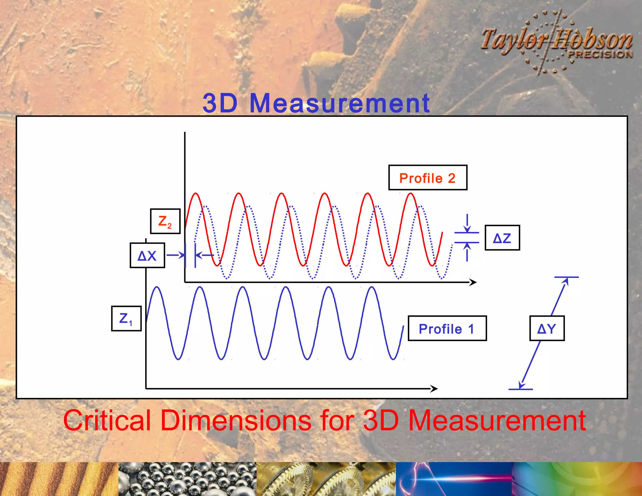
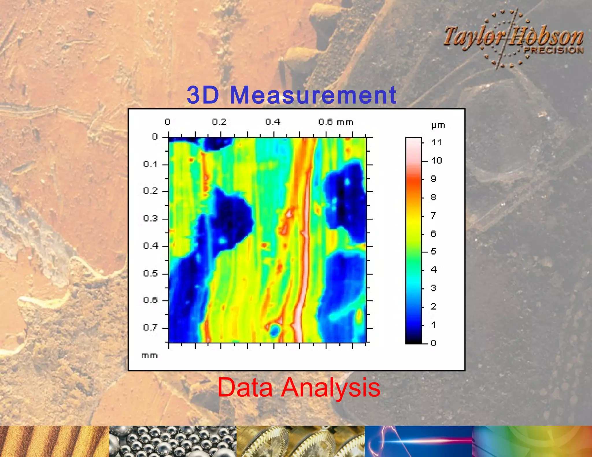
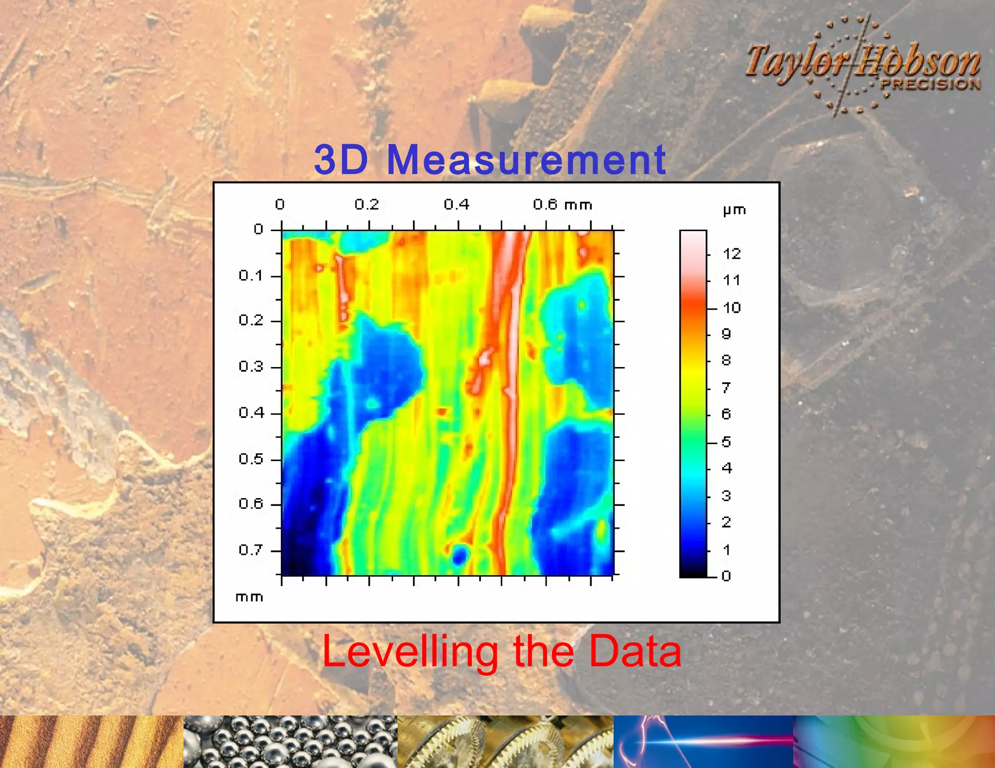
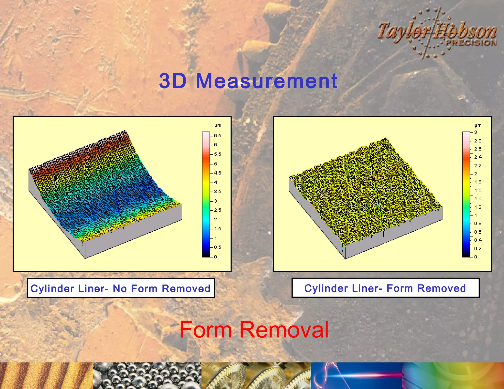
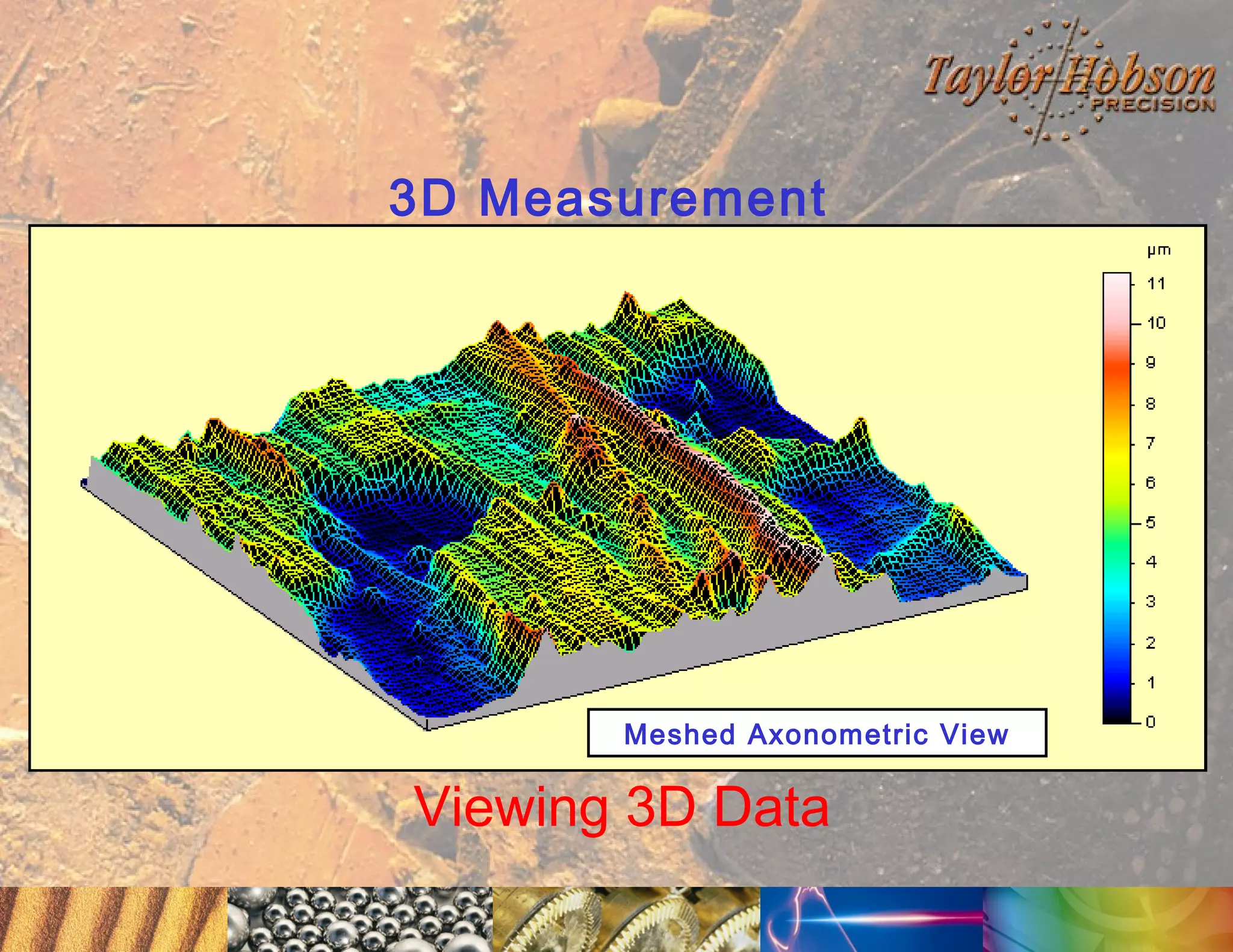
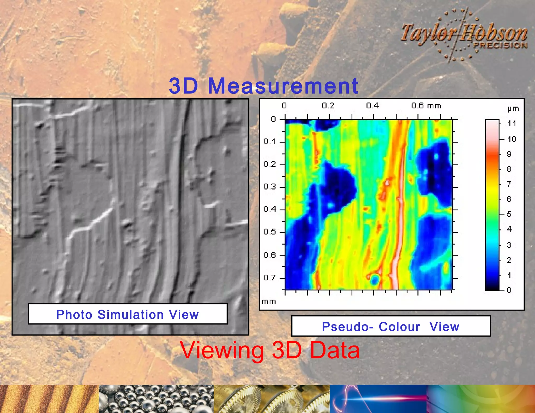
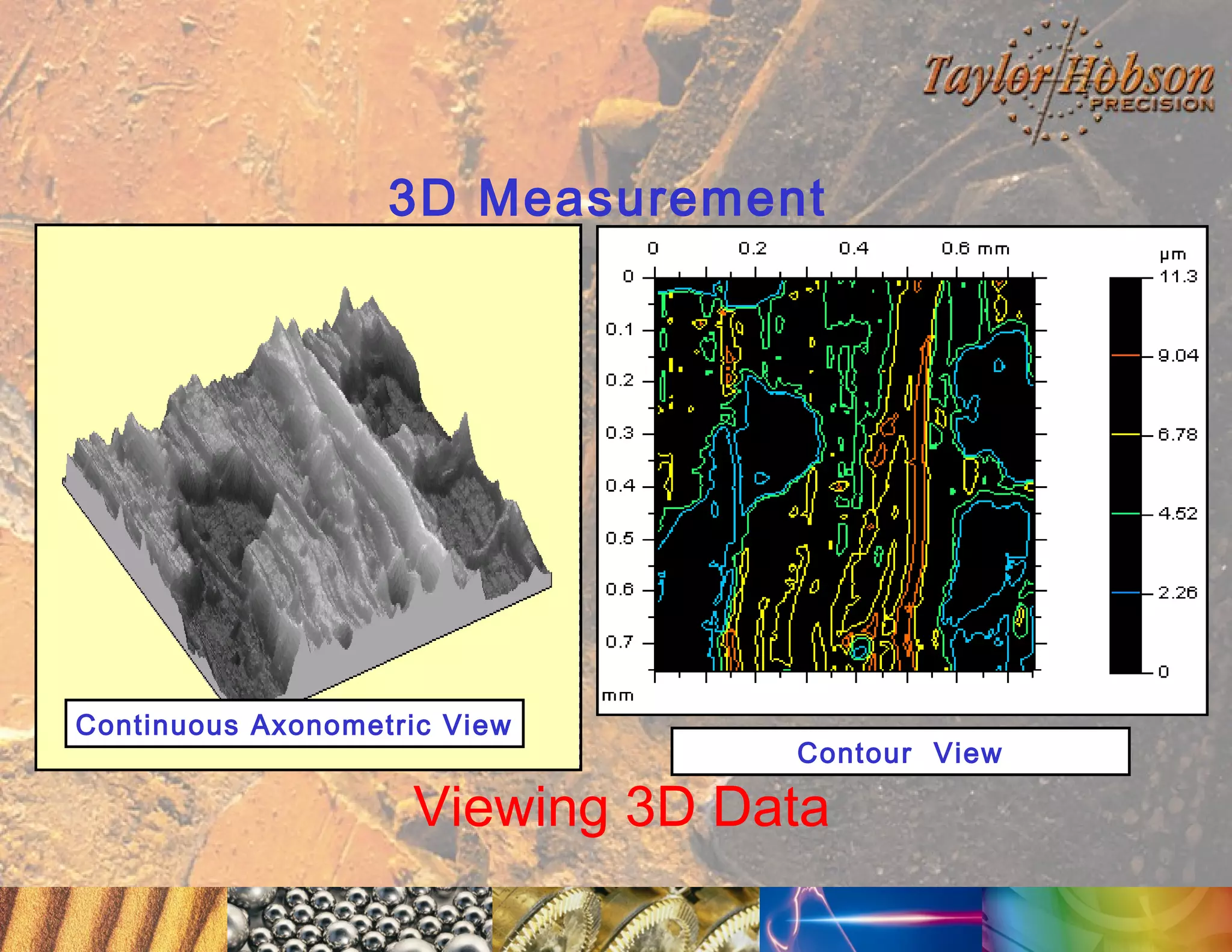
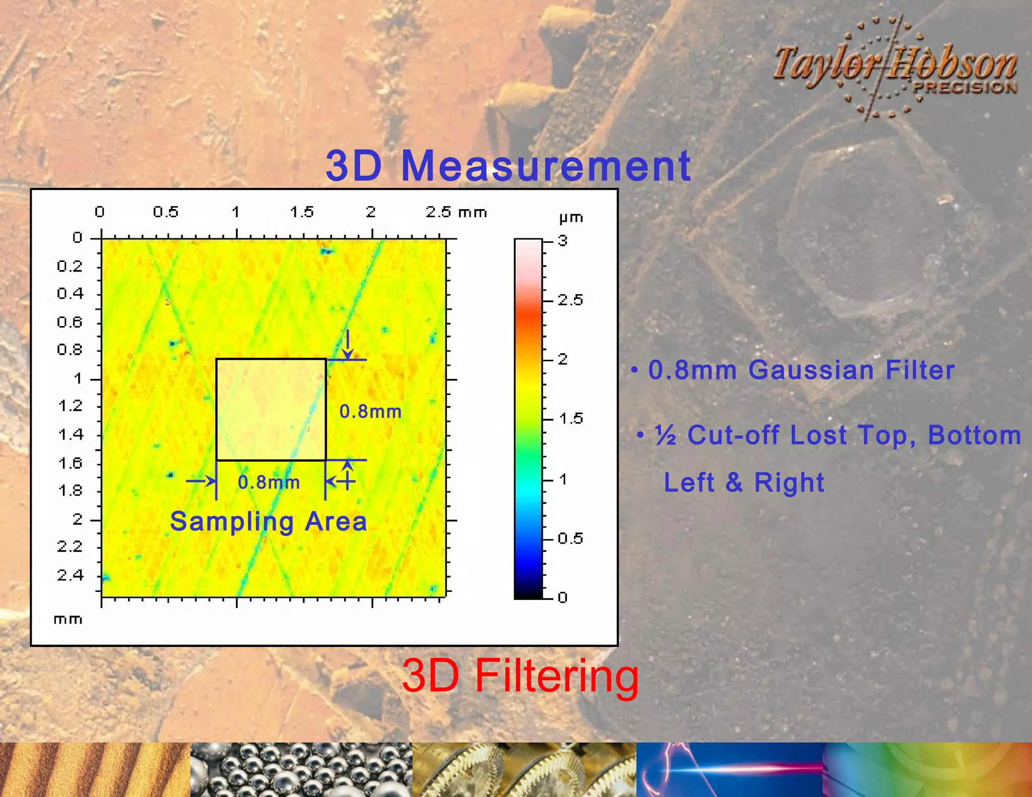
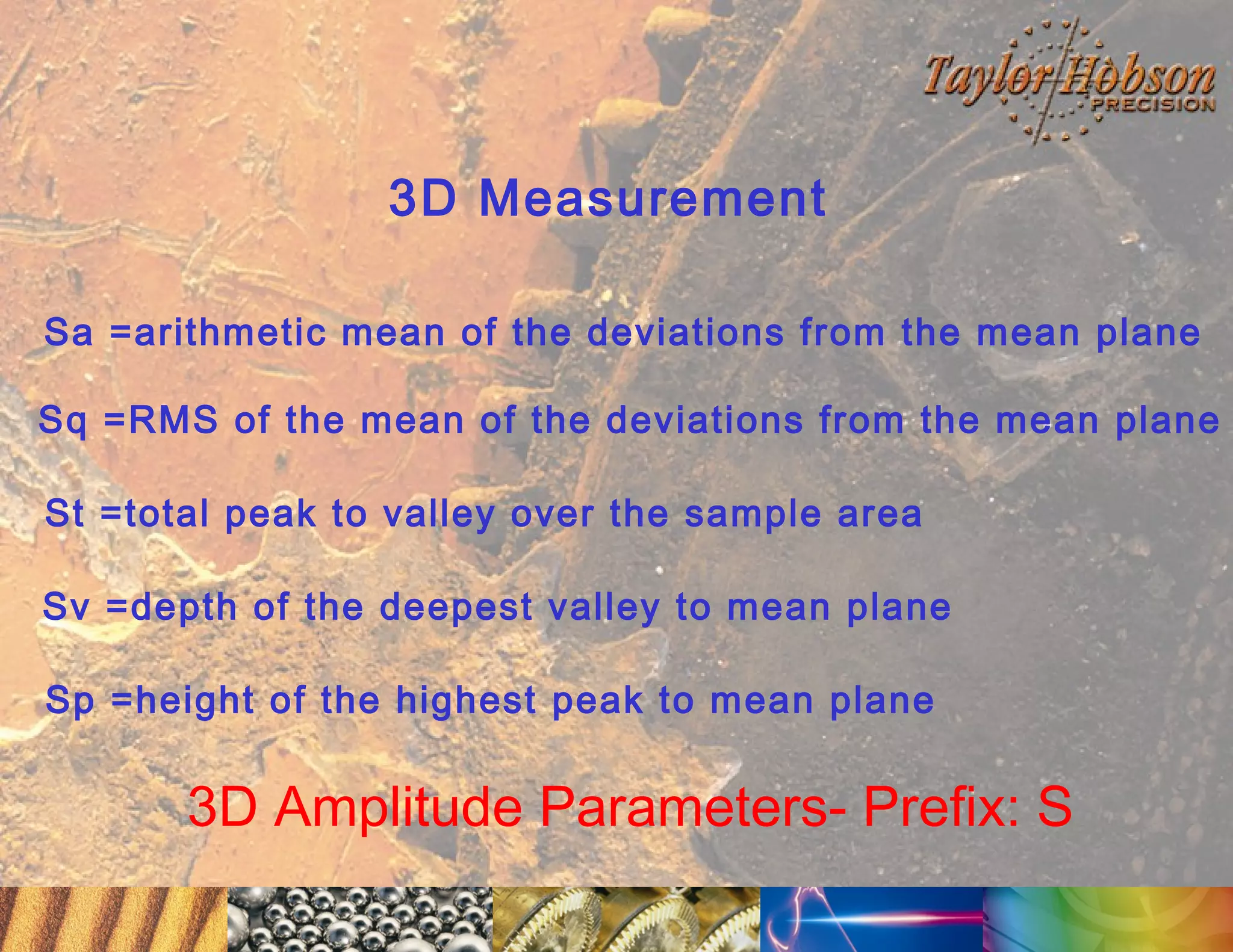
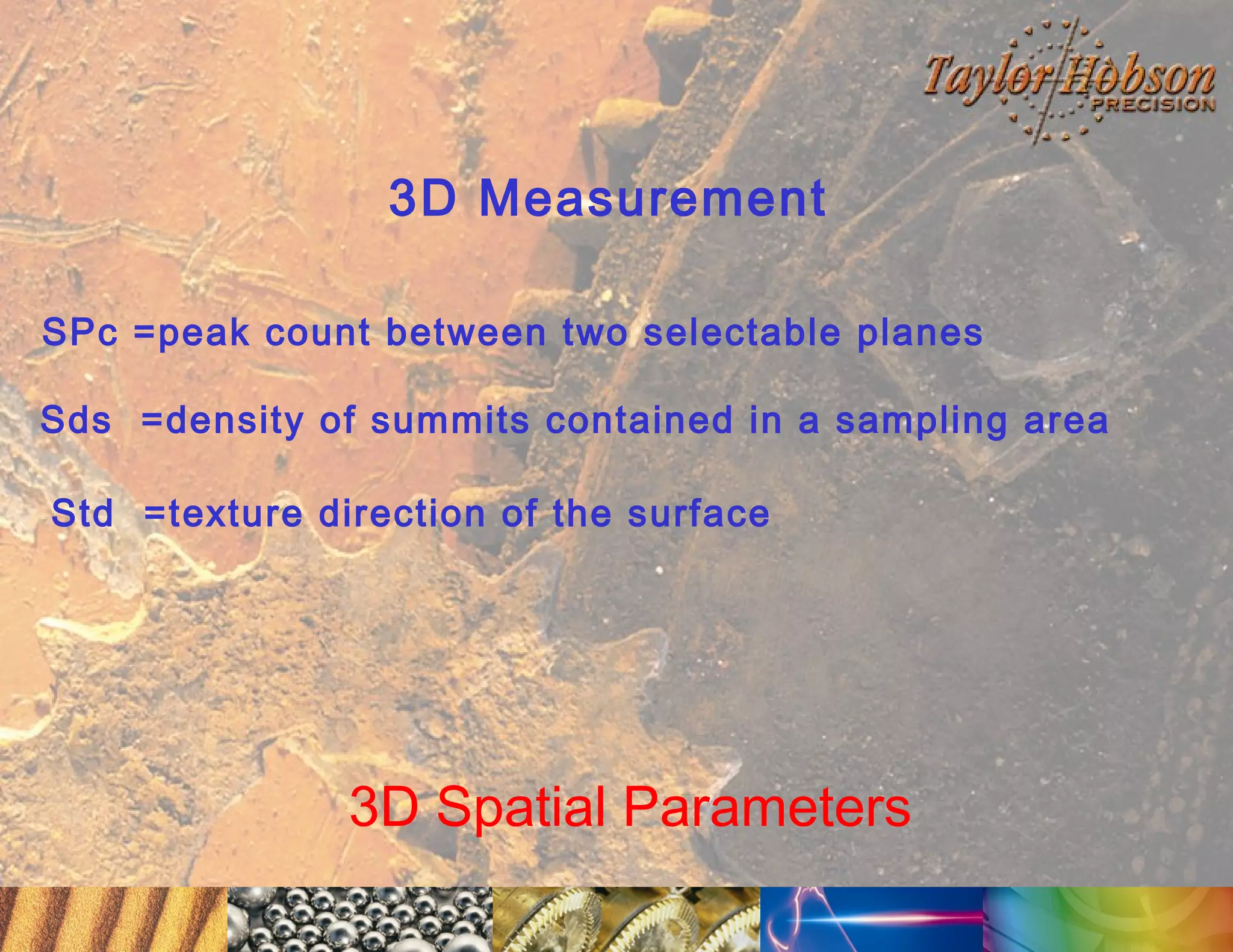
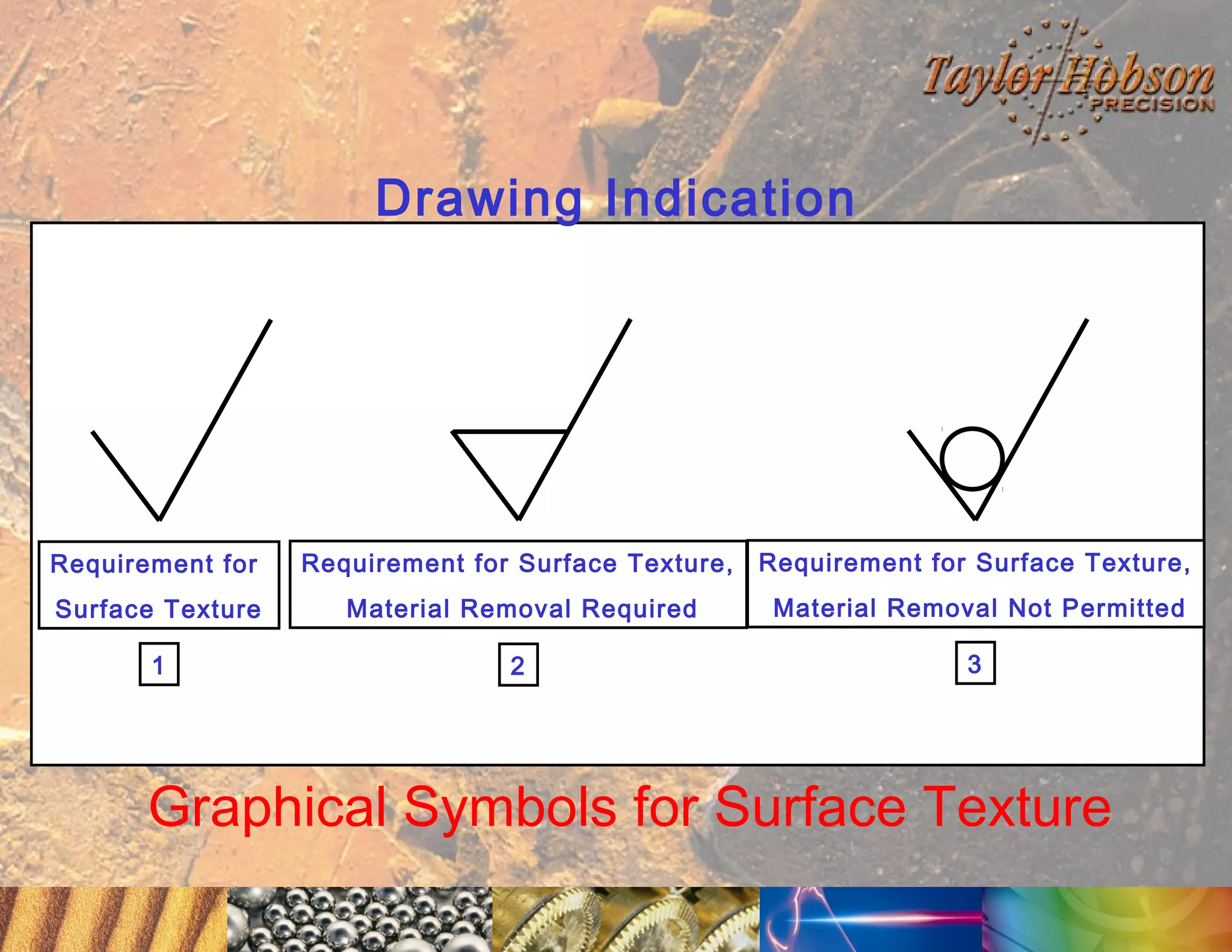
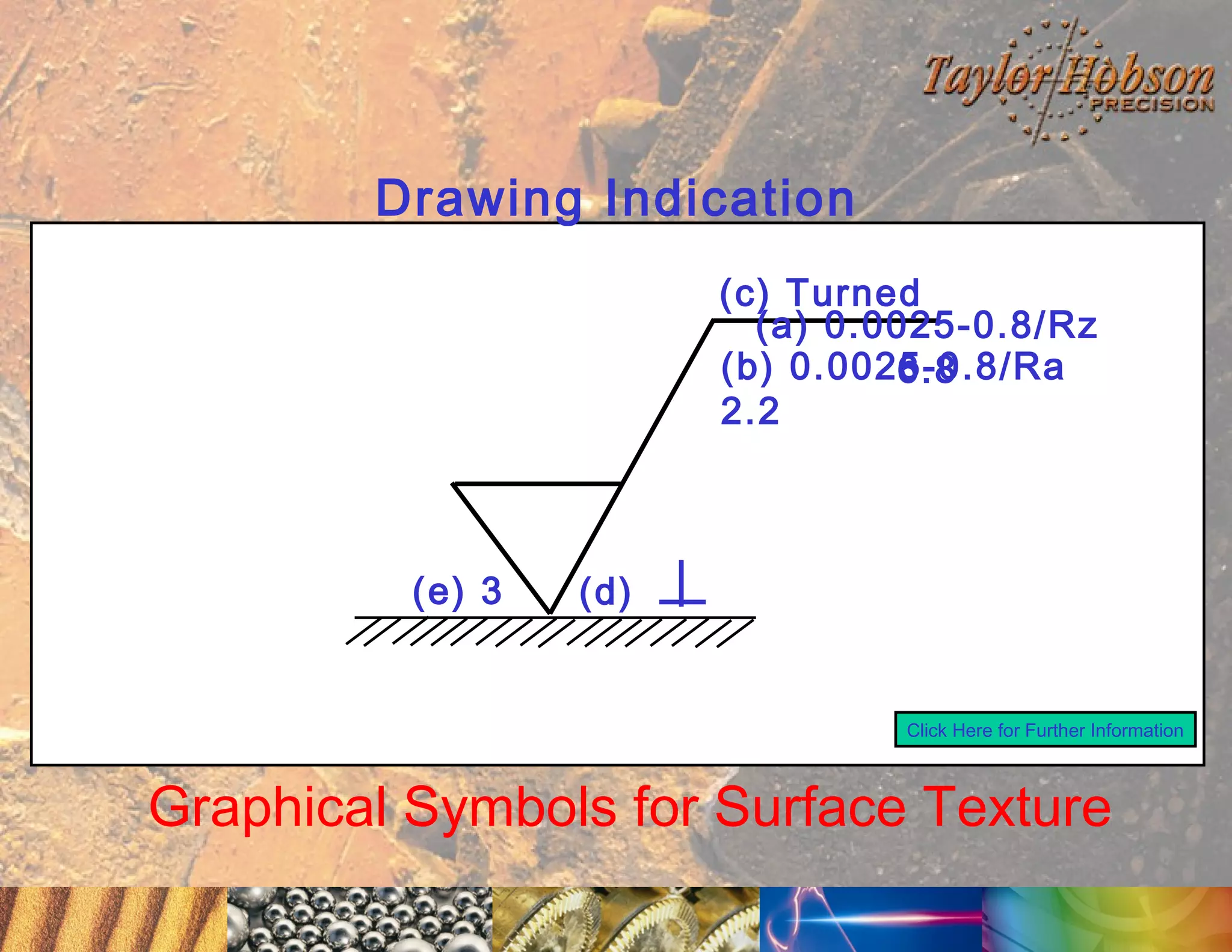
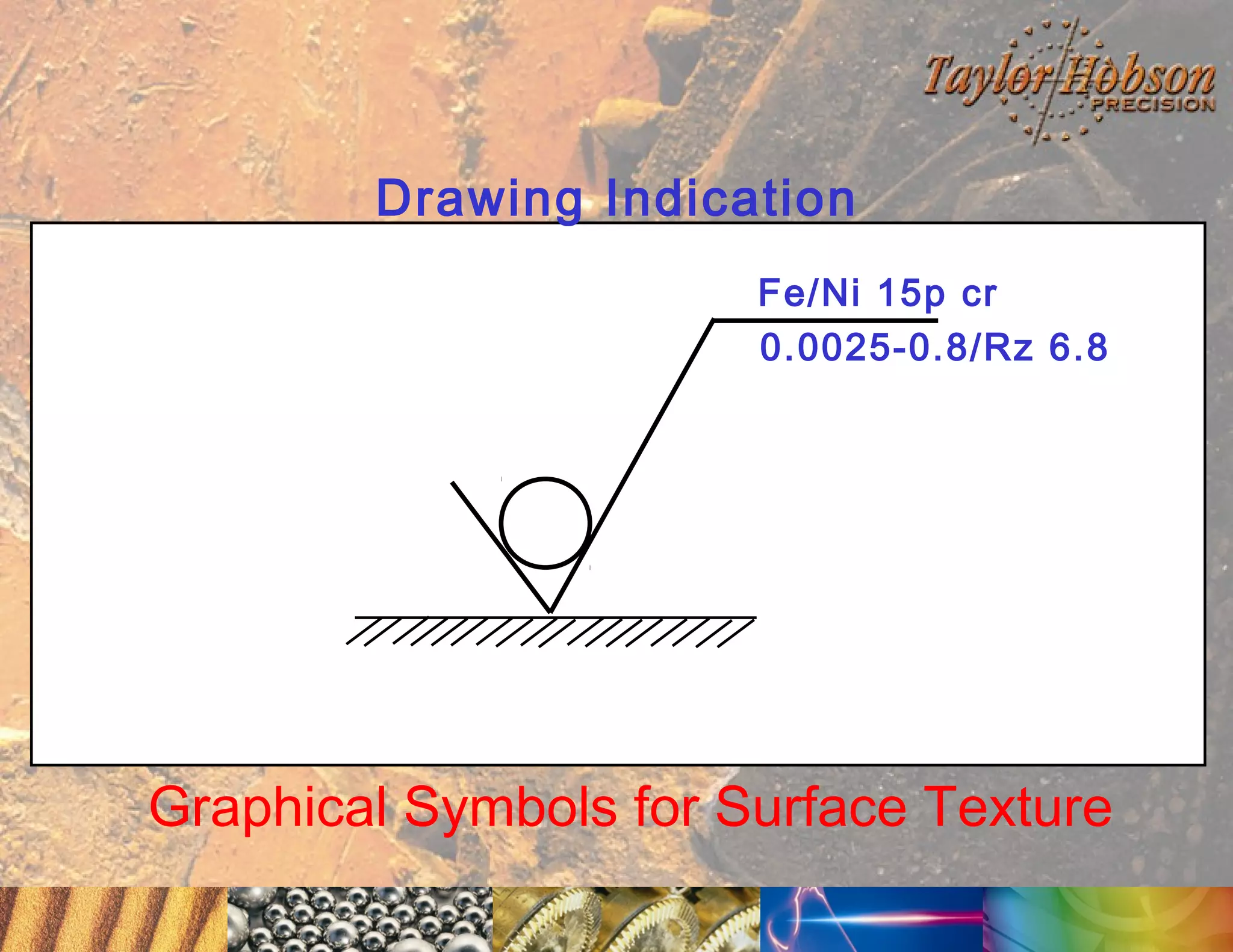
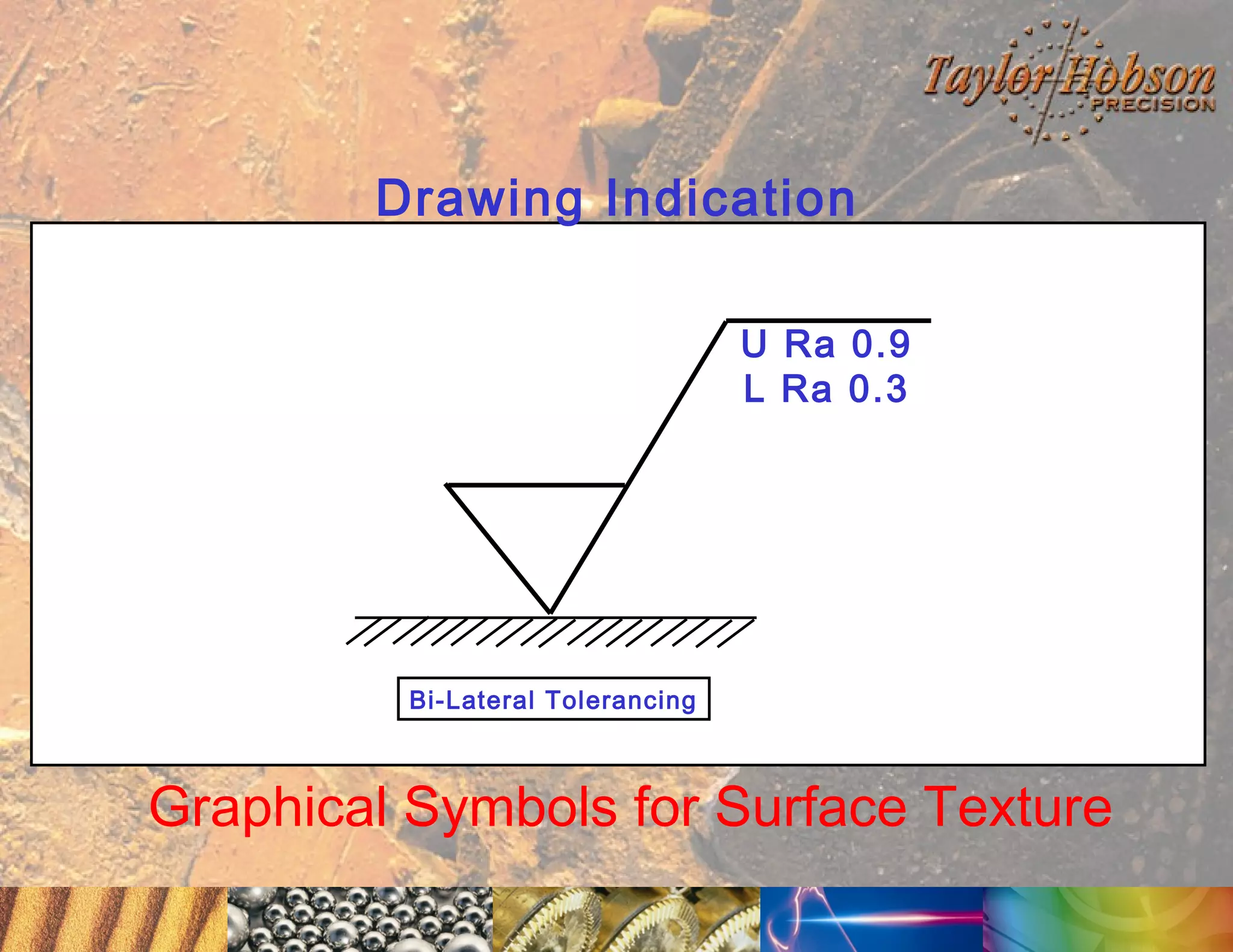
The document discusses surface metrology and measurement. It covers topics such as why surface finish needs to be measured, various measurement methods including contact and non-contact instruments, parameters like roughness and waviness, filters used to separate out different surface components, and calibration methods. Form measurement is also covered, including measurement of parameters like straightness, least squares arcs and radii.

Technology◦Business◦

1 / 178

2 / 178

Surface finish metrology iss1

2.
Contents 1. Why dowe need to measure Surface Finish? 8. Bearing Area (Material Ratio) 2. Measurement Methods 9. The Rk Parameter 3. Measurement Datums 10. Form Measurement 4. Reproducing the Surface 11. Calibration Methods. 5. Terminology 12. Conics and Aspherics. 6. Filters 13. 3D (Areal) Measurement. 7. Parameters 14. Drawing Indication.
3.
Why do weneed to measure Surface Finish?
4.
Nature of Surfaces Themicrostructure of the material
5.
Nature of Surfaces Themicrostructure of the material The action of the cutting tool
6.
Nature of Surfaces Themicrostructure of the material The action of the cutting tool The instability of the cutting tool on the material
7.
Nature of Surfaces Themicrostructure of the material The action of the cutting tool The instability of the cutting tool on the material Errors in machine tool guideways
8.
Nature of Surfaces Themicrostructure of the material The action of the cutting tool The instability of the cutting tool on the material Errors in machine tool guideways Deformations due to stress patterns in the component
9.
Nature of Surfaces Themicrostructure of the material The action of the cutting tool The instability of the cutting tool on the material Errors in machine tool guideways Deformations due to stress patterns in the component
10.
Unwanted Properties ona Surface Deep valleys which may be susceptible to crack propagation Too many peaks which may cause early surface breakdown and wear when in contact with a mating component Excessive waviness which may cause noise or indicate machining problems
11.
Wanted Properties ona Surface Sufficient valleys for oil retention when lubrication is an important factor Sufficient peaks for retention of paint and adhesives Sufficient distribution of valleys for formability Smooth surface profiles for reduced, noise, vibration or high reflectance.
12.
Why Do WeNeed to Measure Surface Finish? Process Control Predicting Component Behaviour Monitoring Component Performance
13.
Why Do WeNeed to Measure Surface Finish? The Ideal Situation
14.
Why Do WeNeed to Measure Surface Finish? The Reality - Process Control
15.
Why Do WeNeed to Measure Surface Finish? Predicting Component Behaviour
16.
Why Do WeNeed to Measure Surface Finish? Back to Contents Page Monitoring Component Performance
17.
Measurement Methods
18.
Measurement Methods Contact TypeInstruments Non-Contact Type Instruments
19.
How Do WeMeasure Surface Finish? Comparison Plates
20.
Measurement Methods Data PointSpacing (X) Stylus Movement (Z) Traverse Direction (X) Contact Type Instrument
21.
Measurement Methods Inductive Typeof Transducer Coil Ferrite Slug (Armature) Beam Coil Stylus Knife Edge Pivots
22.
Measurement Methods Piezo-Electric Typeof Transducer Beam Stylus Piezo Element
23.
Measurement Methods Laser Typeof Transducer Laser Photo Beam Diode Stylus Click Here for Further Information Back to Contents Page
24.
Measurement Datums
25.
Measurement Datums Traverse Direction(X) Skid Stylus Movement (Z) Skid (surface) Datum
26.
Measurement Datums • ReducesEffects of Vibration • No Surface Levelling Required • Instrument Portability • Robust Design Benefits of Using a Skid Datum
27.
Measurement Datums H1 H2 Actual Height Effect ofSkid to Stylus Pitch Apparent Height
28.
Measurement Datums Resultant ProfileP-V = 0µm P-V = 10µm Effect of Skid to Stylus Pitch
29.
Measurement Datums Traverse UnitDatum Traverse Direction Independent Datum
30.
Measurement Datums Traverse UnitDatum Traverse Direction Datum Skid Optical Flat Independent Datum Back to Contents Page
31.
Reproducing the Surface
32.
Reproducing the Surface 2µm TraverseDirection 2µm Conisphere Stylus Truncated Pyramid Stylus Stylus Tip Geometry Click Here for Further Information
33.
Reproducing the Surface StylusTip - Effects of Tip Size & Shape
34.
Reproducing the Surface StylusTip - Flanking
35.
Reproducing the Surface Profileproduced by Stylus B A Stylus Tip B A Stylus Tip - Flanking Back to Contents Page
36.
Terminology
37.
Terminology Data Points True Signal AliasingSignal Sampling Interval Aliasing Click Here for Further Information
38.
Terminology Sample Surface Roughness, Waviness& Form
39.
Terminology Form Roughness, Waviness &Form
40.
Terminology Waviness Roughness, Waviness &Form
41.
Terminology Roughness Roughness, Waviness &Form Back to Contents Page
42.
Filters
43.
Terminology Surface Interaction Filtering-Separates Roughnessand Waviness
44.
Filters Sampling Length Filtering UsingGraphical Techniques
45.
Filters Form Cut-off Sample Ra,Rq,Rz etc... Roughness Filter
46.
Filters Form Cut-off Sample Wa,Wq,Wz etc... Waviness Filter
47.
Filters • ISO 2CR Filter •2CR PC •Gaussian Electronic & Digital Filter Types
48.
Filters Unfiltered Profile ISO 2CRFiltered Profile ISO 2CR Filter Click Here for Further Information
49.
Filters Mean Line Established ByFilter Modified Profile Relative to Filtered Mean Line ISO 2CR Filter Effect
50.
Filters Unfiltered Profile 2CR PCFiltered Profile 2CR PC Filter
51.
Filters Mean Line Established ByFilter Modified Profile Relative to Filtered Mean Line ISO 2CR PC Filter
52.
Filters Unfiltered Profile Gaussian Filtered Profile GaussianFilter
53.
Filters Z Profile Filter Unfiltered Profile MeanLine Cut-off Sampling Length Gaussian Filter X Click Here for Further Information
54.
Filters Unfiltered Profile Roughness Amplitude =20µm Roughness Wavelength = 0.25 mm Waviness Amplitude = 100µm Waviness Wavelength The Effects of Filtering = 8.0 mm
55.
Filters Roughness Amplitude 8.0 mmCut-off filter = 20µm Roughness Wavelength = 0.25 mm Waviness Amplitude = 75µm Waviness Wavelength = 8.0 mm The Effects of 2CR Roughness Filter
56.
Filters 2.5 mm Cut-offfilter Roughness Amplitude = 20µm Roughness Wavelength = 0.25 mm Waviness Amplitude = 24µm Waviness Wavelength = 8.0 mm The Effects of 2CR Roughness Filter
57.
Filters 0.8 mm Cut-offfilter Roughness Amplitude = 20µm Roughness Wavelength Waviness Amplitude = 2µm = 0.25 mm Waviness Wavelength = 8.0 mm The Effects of 2CR Roughness Filter
58.
Filters 0.25 mm Cut-offfilter Roughness Amplitude = 15µm Roughness Wavelength Waviness Amplitude = 0µm = 0.25 mm The Effects of 2CR Roughness Filter
59.
Filters 0.08 mm Cut-offfilter Roughness Amplitude = 4µm Roughness Wavelength Waviness Amplitude = 0µm = 0.25 mm The Effects of 2CR Roughness Filter
60.
Filters Traverse Length Over travel Run-up SamplingLength (Cut-off) Assessment (Evaluation) Length Relationship of Sampling, Assessment & Traverse Length (ISO 2CR)
61.
Filters • ISO 2CR-1st 2 Cut-offs discarded • 2CR PC- 1st & Last Cut-offs discarded •Gaussian- Half 1st & Half Last Cut-off Discarded Filter Types
62.
Filters 0.8mm Sampling Length (Cut-off) Cut-offSelection
63.
Filters 0.25mm Sampling Length (Cut-off) Cut-offSelection
64.
Filters Traverse Direction 1.25 mm Choosingthe Correct Cut-off Value
65.
Filters Cut-off Selection Unless otherwiseindicated on a drawing the table above should be used to determine the cut-off
66.
Filters Ls Lc Bandwidth=Ratio of Lc/Ls Backto Contents Page
67.
Parameters
68.
Parameters •Roughness - Prefix R •Waviness- Prefix W •Primary - Prefix P Analysis Types
69.
Parameters •Amplitude Parameters defined fromZ co-ordinates Parameter Types
70.
Parameters • Amplitude Parameters definedfrom Z co-ordinates • Spacing Parameters defined from X co-ordinates Parameter Types
71.
Parameters • Amplitude Parameters definedfrom Z co-ordinates • Spacing Parameters defined from X co-ordinates • Hybrid Parameters X & Z co-ordinates Parameter Types
72.
Parameters Ra Amplitude Parameters -Ra
73.
Parameters Ra Ra Ra Ra Amplitude Parameters -Limitations of Ra
74.
Parameters lr =Sampling Length AmplitudeParameters Rq (RMS)
75.
Parameters lr =Sampling Length ln=Assessment Length Amplitude Parameters Rt
76.
Parameters Sampling Length Amplitude ParametersRp
77.
Parameters Sampling Length Amplitude ParametersRv
78.
Parameters Rz 2 Rz 1 Rz3 Rz 4 Rz 5 Rz = Maximum peak to valley in each sample length divided by n sampling lengths Amplitude Parameters Rz
79.
Parameters Rp1ma x Rz1max Rv1max Amplitude Parameters Rz1max,Rp1max & Rv1max
80.
Parameters A=Slice level lr =SamplingLength (Cut-off) B= Mean Line ln =Assessment Length Spacing Parameters HSC (High Spot Count)
81.
Parameters Tall narrow peakstend to work harden Hardened peaks will eventually break off and the surface will breakdown Spacing Parameters HSC (High Spot Count)
82.
Parameters A=Selectable Bandwidth B= Mean Line SpacingParameters Rpc (Peak Count)
83.
Parameters Painted Surface Base SheetSteel Orange Peel Effect Due to Peaks on Sheet Steel Base Surface Spacing Parameters Rpc (Peak Count)
84.
Parameters Mean Line lr =SamplingLength (Cut-off) Spacing Parameters Sm (Mean Spacing)
85.
Parameters θ θ θ θ Hybrid Parameters- Rdq(Pdq, Wdq) (Rms Slope)
86.
Parameters Effects of SurfaceSlopes on vibration & noise No Vibration/Quiet Low Frequency Rumble High Frequency Scream Hybrid Parameters- Rdq (Pdq, Wdq) (Rms Slope)
87.
Parameters With low surfaceslopes more light is reflected into the eye and hence has a good appearance With high surface slopes less light is reflected into the eye and hence has a poor appearance Hybrid Parameters- Rdq (Pdq, Wdq) (Rms Slope) Back to Contents Page
88.
Bearing Area (Material Ratio)
89.
Bearing Area (MaterialRatio) Upper surface defines run-in characteristics Body of surface defines wear/life characteristics Valleys define lubrication characteristics Hybrid Parameters - Rmr
90.
Bearing Area (MaterialRatio) Lapping Plate Bearing Line Rmr= a+b+c+d+e ln x100 ln =Assessment Length Hybrid Parameters - Rmr
91.
Bearing Area (MaterialRatio) Level p Tp (%) at level p 0 tp(%) Material Ratio Curve (Rmr) 100 %
92.
Bearing Area (MaterialRatio) Level p Tp (%) at level p 0 tp(%) Material Ratio Curve (Rmr) 100 %
93.
Bearing Area (MaterialRatio) Level p Tp (%) at level p 0 tp(%) Material Ratio Curve (Rmr) 100 %
94.
Bearing Area (MaterialRatio) Level p 0 Number of Peaks Amplitude Distribution Curve Click Here for Further Information
95.
Bearing Area (MaterialRatio) Surface with Random Amplitude DistributionSurface with RandomSkew Zero Amplitude DistributionZero Skew Associated MR Curve Parameters-Rsk (Skew)
96.
Bearing Area (MaterialRatio) Surface with dominant peaks-Positive Skew Associated MR Curve Parameters-Rsk (Skew)
97.
Bearing Area (MaterialRatio) Surface with dominant valleys-negative Skew Associated MR Curve Parameters-Rsk (Skew)
98.
Bearing Area (MaterialRatio) Rku<3 Rku=3 Rku>3 Associated MR Curve Parameters-Rku(Kurtosis) Back to Contents Page
99.
The Rk Parameter
100.
Parameters Surface Interaction Rk Parameter
101.
Bearing Area (MaterialRatio) Material Ratio curve Tilted Profile 0 tp(%) Material Ratio Curve (Rmr) 100 %
102.
Parameters Mean Line Unfiltered RealProfile Rk Parameter
103.
Parameters Valleys removed &kept in memory Unfiltered Real Profile after valley suppression Rk Parameter Mean Line
104.
Parameters Final Filtered RoughnessProfile Rk Parameter
105.
Parameters 40 % Rdc 0 Rk Parameter tp(%) 100%
106.
Parameters 40 % C E A Rdc B 0 tp(%) F D 100 % RkParameter
107.
Parameters 40 % C E Rk A Rdc B D1 D Mr2 Mr1 0 F tp(%) 100 % RkParameter
108.
Parameters 40 % C Rk Rpk C E D E A B D1 Area 1 Rvk FD E Mr2 Mr1 0 Rdc tp(%) 100 % Rk Parameter Area 2
109.
Parameters 40 % Rpk Rk Rvk Mr2 Mr1 0 tp(%) 100 % RkParameter
110.
Parameters • Rk-Core RoughnessDepth • Rpk-Reduced Peak Height • Rvk-Reduced Valley Depth • Mr1-Material Component Relative to Peaks • Mr2-Material Component Relative to Valleys • A1-Material Filled Profile Peak Area • A2-Lubricant Filled Profile Valley Area Rk Associated Parameters Back to Contents Page
111.
Form Measurement
112.
Form Measurement Least SquaresLine
113.
Form Measurement Straightness (LSLine)
114.
Form Measurement Straightness (MZLine)
115.
Form Measurement r r R=Calculated LSRadius r-r=LS Arc Least Squares Arc
116.
Form Measurement t=34.501656mm l=80mm r-t r=110mm t= ChordalHeight r= Least Squares Radius l= Measurement Length/2 Least Squares Arc - Radius Measurement
117.
Form Measurement t=1.833462mm l=20mm r-t r=110mm t= ChordalHeight r= Least Squares Radius l= Measurement Length/2 Least Squares Arc - Radius Measurement
118.
Form Measurement t=1.833962mm l=20mm r=109.9705mm t= ChordalHeight r= Least Squares Radius l= Measurement Length/2 Least Squares Arc - Radius Measurement Back to Contents Page
119.
Calibration Methods
120.
Calibration Methods Traverse Direction BallStandard
121.
Software Corrections Traverse Direction dZ dX ArcuateErrors
122.
Software Corrections Traverse Direction Pathof Stylus Tip Centre Stylus Tip Errors
123.
Calibration Methods Ra &Rz Roughness Standards
124.
Calibration Methods Ra &Rz Roughness Standards
125.
Calibration Methods Traverse Direction 2.5µmStep Height 3 Line (Step Height) Standard
126.
Calibration Methods A=Mean Line B=CalibrationHeight 3 Line (Step Height) Standard
127.
Calibration Methods A=Level Surface C=UnlevelledSurface B=Pt Value Click Here for Further Information Back to Contents Page 3 Line (Step Height) Standard
128.
Conics & Aspherics
129.
Conics and Aspherics ConicSections
130.
Conics and Aspherics Ellipse:K< 0 Sphere: K= 0 Oblate Ellipse: K>0 Z2 + X2 = 1 R2 2 R1 2 Z2 + X2 = 1 R2 R2 Z2 + X2 = 1 R2 2 R1 2 Conic Constants
131.
Conics and Aspherics Hyperbola:K< -1 Parabola: K= -1 Z2 + X2 = 1 R2 2 R1 2 Z = (Ax) 2 Conic Constants
132.
Conics and Aspherics ConventionalSpherical Lens What is an Aspheric?
133.
Conics and Aspherics AsphericLens What is an Aspheric?
134.
Conics and Aspherics •Reduces Spherical Aberration • Ability to Produce Vari-focal Lenses • Reduction in Lens Size and Weight • Greater Design Freedom Reasons for using an Aspheric
135.
Z Axis Conics andAspherics Basic Conic Section (Sphere) Z2 + X2 = 1 R2 R2 X Axis How is an Asphere constructed?
136.
Z Axis Conics andAspherics Basic Conic Section (Sphere) Aspheric Polynomial Curve Z=a 8 |x| 8 X Axis How is an Asphere constructed?
137.
Z Axis Conics andAspherics Aspheric Profile Basic Conic Section (Sphere) Aspheric Polynomial Curve C B A How is an Asphere constructed? X Axis
138.
Z Axis Conics andAspherics Aspheric Profile Aspheric Profile Basic Conic Section (Sphere) Basic Conic Section C B Aspheric Polynomial Curves Aspheric Polynomial Curve A X Axis How is an Asphere constructed?
139.
Conics and Aspherics cx2 Z(x)= 1+ √ 1 -(K+1) c 2 x 2 +a 1 |x| +a 2 | x| 2 + a 3 | x| 3 … +a 20 | x| 20 Where: X is the Radial distance from the Aspheric Axis Z is the corresponding vertical distance a is the indexed Polynomial Coefficient C is the reciprocal of the Base Radius K is the Conic Constant of the Surface Standard Equation for An Aspheric Surface
140.
Conics and Aspherics BaseRadius of Curvature
141.
Conics and Aspherics AsphericAxis Optical Flat How Do We Measure an Aspheric Surface?
142.
Conics and Aspherics AsphericData Radius=40.0mm K= -1 A4= 5.3188e-007 A6=5.5231e-009 A8=-1.6774e-011 A10=-6.3352e-014 How Do We Analyse an Aspheric Surface?
143.
Conics and Aspherics ZAxis B A Aspheric Axis Aspheric Form Fit X Axis
144.
Conics and Aspherics +ZAxis Aspheric Axis A +X Axis -X Axis -Z Axis Aspheric Axis Residual Error after Aspheric Form Removal
145.
Conics and Aspherics HowDo We Analyse an Aspheric Surface?
146.
Conics and Aspherics AsphericParameters
147.
Conics and Aspherics ConvexComponent-Concave Residual Form Error-Increase Base Radius Aspherics-Further Analysis
148.
Conics and Aspherics ConvexComponent-Convex Residual Form Error-Decrease Base Radius Aspherics-Further Analysis
149.
Conics and Aspherics SmallestRt Value Achieved-True Shape & Base Radius Aspherics-Further Analysis Back to Contents Page
150.
3D (Areal) Measurement
151.
3D Measurement • GoodVisualisation of the Surface • More Statistically Stable • Better at Detecting & Analysing Defects • Many Methods of Representing the Data Advantages of 3D (Areal) over 2D
152.
3D Measurement • Longermeasurement cycles • Measurement Produces Large Data Files • Mainly Restricted to R & D • Sometimes Visually Subjective Disadvantages of 3D (Areal)
153.
3D Measurement Traverse Direction YAxis Incremental Movement Contact Measurement Method
154.
3D Measurement CCD Detector Laser YAxis Incremental Movement Measurement Axis (X) Non-Contact Measurement Method
155.
3D Measurement Profile 2 Z2 ΔZ ΔX Z1 Profile1 ΔY Critical Dimensions for 3D Measurement
156.
3D Measurement Data Analysis
157.
3D Measurement Levelling theData
158.
3D Measurement Cylinder Liner-No Form Removed Cylinder Liner- Form Removed Form Removal
159.
3D Measurement Meshed AxonometricView Viewing 3D Data
160.
3D Measurement Photo SimulationView Pseudo- Colour View Viewing 3D Data
161.
3D Measurement Continuous AxonometricView Contour View Viewing 3D Data
162.
3D Measurement • 0.8mmGaussian Filter 0.8mm • ½ Cut-off Lost Top, Bottom Left & Right 0.8mm Sampling Area 3D Filtering
163.
3D Measurement • Amplitude •Spatial • Hybrid • Functional 3D Parameter Types
164.
3D Measurement Sa =arithmeticmean of the deviations from the mean plane Sq =RMS of the mean of the deviations from the mean plane St =total peak to valley over the sample area Sv =depth of the deepest valley to mean plane Sp =height of the highest peak to mean plane 3D Amplitude Parameters- Prefix: S
165.
3D Measurement SPc =peakcount between two selectable planes Sds =density of summits contained in a sampling area Std =texture direction of the surface 3D Spatial Parameters
166.
3D Measurement SΔq =RMSslope of the surface Ssc =mean summit curvature of the surface Sdr =developed interfacial area ratio of the surface 3D Hybrid Parameters
167.
3D Measurement Stp=surface bearingarea ratio Sbi =surface bearing index Sci =core fluid retention index Svi =valley fluid retention index 3D Functional Parameters
168.
3D Measurement Volume/Defect Analysis
169.
3D Measurement Step HeightAnalysis
170.
Drawing Indication
171.
Drawing Indication 6.8 Conventional SurfaceTexture Symbol Graphical Symbols for Surface Texture
172.
Drawing Indication Requirement for Requirementfor Surface Texture, Requirement for Surface Texture, Surface Texture Material Removal Required Material Removal Not Permitted 1 2 3 Graphical Symbols for Surface Texture
173.
Drawing Indication (c) Turned (a)0.0025-0.8/Rz (b) 0.0025-0.8/Ra 6.8 2.2 (e) 3 (d) Click Here for Further Information Graphical Symbols for Surface Texture
174.
Drawing Indication Fe/Ni 15pcr 0.0025-0.8/Rz 6.8 Graphical Symbols for Surface Texture
175.
Drawing Indication U Ra0.9 L Ra 0.3 Bi-Lateral Tolerancing Graphical Symbols for Surface Texture
176.
Drawing Indication • Nomore than 16% of the measured values for an upper limit should exceed the specified value • No more than 16% of the measured values for a lower limit should be less than the specified value The 16% Rule (Default Rule)
177.
Drawing Indication RzMAX 0.9 TheMAX Rule
178.
End Back to ContentsPage

Editor's Notes

#10 The highlighted points are the main areas of measurement when looking at surface finish (roughness). These are the irregularities on the surface of a component that remain after a machining process. Generally the surface finish (roughness) comprises of the traverse feed marks produced by the cutting tool as seen on a turned or ground component.
#11 All of the previous elements that characterise the surface could cause the undesirable effects shown depending on how the component is used. For example if a surface is to be used for a brake liner then it needs to create friction and would be useless if it were smooth. Alternatively if a surface was to be used in a bearing then friction would be undesirable.
#12 These properties are closely linked to the function of the component. If two surfaces are moving in contact with each other then there is a need for sufficient lubricant retention on the surfaces to prevent seizure or rapid wear of the two surfaces. Conversely if there is a requirement for a surface to have good adhesive properties, such as sheet steel used for forming panels on a car body, then the paint must be able to bond to the surface without producing any “orange peel” effects, therefor the surface must have sufficient peaks to allow the paint to bond. A sheet steel surface surface that has predominately valleys will have the ability to be formed much easier the a surface with predominately peaks. Low sloping surface profiles will produce less vibration and noise which would be a requirement of a bearing surface. The cosmetic appearance of a surface will improve if it has a low sloping profile.
#13 The three points shown are the main reasons why we need to measure surface finish. In an ideal world we would like to be able to manufacture large batches of components of the same design correctly time after time and each one performs correctly. The reality, however, is rather different.
#14 If a manufacturing process remained constant all components produced within the design specification would perform correctly and there would be no need to measure the surface finish.
#15 In reality this ideal situation as we are aware does not always happen. No manufacturing process will remain constant. Some irregularities, of varying degrees, will be produced in the manufactured surface by the action of the cutting tool or the instability of the cutting tool on the material. As a consequence we have to insert an extra step in the manufacturing process. This is the measurement/ process control step. This step will help to identify any deviations of the surface that fall outside the design specification, which may affect the performance of the component. Once a measurement has been made and the component has been found to be outside of the required specification, scrapping the component and continuing with production would be uneconomical and a waste of time. Identifying the cause of the failure and correcting the manufacturing process will reduce costs and save time.
#16 Future behaviour of the component can be predicted by taking a surface finish measurement. For example, as we have previously mentioned, a surface that has been identified as having predominately valleys will have good oil or lubricant retaining properties. Therefor, if we can measure the quantity and depth of the valleys this will allow us to predict how well the surface will retain lubricants and consequently how quickly the surface will wear.
#17 The performance is not only a mechanical function of the surface, as well as performing correctly, it must also be possible to produce the component economically in the correct quantities within the design specification. There could be a tendency to over engineer the surface finish if it is not measured and monitored during the manufacturing process, incurring unnecessary expense and wasted time.
#19 The two types of instrumentation used for the assessment of surface finish are the contact and non-contact type of instrument.
#20 A basic method of surface finish measurement is by using a comparison plate. These plates consist of a range of metal blocks which have been machined to give various calibrated surface finish values. A components surface can be compared against these machined blocks either visually or by touch. Obviously this method of measurement is a bit subjective. Using this method it is difficult to attach an absolute value to a surface. The various surfaces on these plates are usually identified with Roughness Grade Numbers, N12 to N1. These grades correspond to nominal preferred Ra values. N12 would be an Ra value of 50µm, N1 a value of 0.0125µm Ra. Note: The N grades used in the USA are not identified in the same way as the European grades shown above.
#21 The contact type of instrument consists of a stylus which tracks across the surface under test. A gauge or pick-up which is a transducer that translates the movements of the stylus in the Z (height) direction as it tracks across the surface (X axis) into a usable electronic signal. This signal is then processed via software to present the operator with a value which represents the surface finish. The traverse mechanism will also provide X co-ordinate positions of the surface data by using a grating which has a fixed spacing. The Form Talysurf Series instrument has data point spacing in the X axis of 0.25µm (1µm for traverse lengths greater than 30mm). Another method of data point collection is by utilising the motor driving the traverse unit. This method involves some form of positional feedback from the motor. Because the speed of the motor is known the position of the stylus can be determined at a set time period during the measurement, which dictates the data point spacing. This method, however, relies on the motor speed being constant to give accurate spacing between data points. An instrument which uses a fixed grating will always give a consistent data point spacing.
#22 The stylus is located at one end of a beam which pivots on knife edges, the other end of the beam consists of a coil with a ferrite slug (armature) which moves inside two coils causing a change in relative inductance. As the stylus moves down a valley the ferrite slug will rise, when the stylus rides up a peak the slug will move down. Each coil therefore represents negative or positive movement of the stylus. The stylus remains in contact with the surface and the knife edges by using a fine spring which acts on the beam. The Form Talysurf Series( S4 ) incorporates this system, the ferrite slug is connected to the end of the stylus.
#23 The piezo-electric transducer contains a piezo-electric crystal element which has the property of developing a voltage across electrodes on the faces of the elements when the crystal is deformed. Again the movement of the stylus creates a bending moment the subsequent voltage output is translated into Z co-ordinates. This type of transducer is used in the Surtronic Duo instrument.
#24 On this type of transducer an end reflector is fixed on the end of pivoted stylus beam which acts as a moving arm for a miniature laser interferometer. The system utilises the laser wavelength as a reference for the measurement. Stylus deviations move a second light path, the change in phase of the wavelengths of one path to another are detected by the photo diode and are translated into surface deviations. This system is used on the Form Talysurf Series ( S5 ) and has a wide dynamic range, achieved by use of the laser interferometric system.
#26 Transducing the gauge movement cannot be done without using some form of fixed reference, i.e. a skid. The movement of the armature within the coils of the gauge is proportional to the stylus movement only if the coils remain stationary with respect to the plane of the surface, therefore, the gauge must traverse along a line parallel to the surface. This will then create a height difference between the skid and the stylus as the gauge traverses the surface. Providing the radius of the skid is larger than the spacing of the surface peaks then the line of traverse will be almost a straight line. The skid radius should ideally be not less than 50 times the nominal cut-off wavelength used. (See Cut-off section) This type of datum is used on the Surtronic range of instruments.
#27 Any vibration on a surface under test will effect both the stylus and skid (datum) simultaneously, reducing the effects of vibration. No levelling would be required because the stylus and skid are traversing the surface together. Depending on the radius of the skid being used this will produce some filtering effect as the skid rides across the top of the surface.
#28 Skid datums can exhibit errors on wavy surfaces. In this example we can see what happens if the skid to stylus tip pitch is equal to half the waviness wavelength of the surface. The apparent or resultant height is twice that of the actual height. An instrument with this type of datum should not be used for measuring waviness or for measuring surfaces that have large waviness profiles.
#29 In this example we can see what can happens when the skid to stylus pitch is equal to the waviness wavelength of the surface. Because there is no height difference between the stylus tip and the skid as the gauge traverses over the surface the resultant profile will display a peak to valley result of zero.
#30 The type of independent datum most commonly found in a surface finish instrument is a ground datum bar. This bar can either be rectangular or round in cross section and is machined to a very high straightness accuracy, usually in the order of 0.5µm over 120mm. This type of datum is found in the Form Talysurf series of instruments. Using this type of datum allows the operator to measure, form waviness and surface finish as well as radius and angle.
#31 An alternative type of independent datum can be produced by utilising an optical flat as shown in this diagram. The flat datum produced by the optical flat is positioned below the gauge and is set parallel to the measurement surface. With this set-up the skid is attached to the underside of the gauge and traverses on the datum surface (optical flat) independently of the measurement surface.
#33 These two diagrams shown the two basic types of stylus tip shape. The 90° diamond tip conisphere and the 90° diamond tip, truncated pyramid. The truncated pyramid has a flat tip with a 2µm tip width in the traverse direction. This is designed in this way to give added strength to the stylus tip but this means that the tip is only useful in the single direction. The conisphere stylus, which has a spherical tip, can be used at 90° to the normal traverse direction whilst still having the correct stylus presentation to the surface. This is particularly useful for measuring difficult radii such as the fillet radii on crankshafts. The conisphere stylus can also have a 5µm tip and/or a 60° tip.
#34 The radius and angle of the stylus tip in relation to the measured surface may effect the accuracy of the measurement. On a surface with deep and narrow valleys the stylus may not be able to reach the bottom of the profile, this produces a mechanical filtering effect on the surface. The greater the stylus tip radius and the larger the cone angle means the tip will make contact with the surface less frequently. Care should be taken when measuring surfaces with an Ra value of < 0.5µm and an Rz value of < 3µm using a 5µm or 10µm stylus tip.
#35 A flanking error may occur when the stylus is traversed over a component profile that includes either a slope or an arc section, any part of which presents a tangential angle greater than 35° for a 90° diamond tipped stylus.
#36 This slide also demonstrates the error cased by stylus flanking on sharp profiles and parts of profiles where the stylus tip is unable to penetrate the profile, producing a rounding off of peaks and an apparent reduction of depth of valleys.
#38 The signal produced by the gauge as the stylus traverses the surface has to be sampled at a fixed sampling interval to produce co-ordinates in the X and Z axes. If this interval is slightly different from the wavelength of the surface a false wavelength will be produced. This error is known as aliasing. To conform to the ISO recommendations a minimum of five data points per wavelength should be taken to obtain a more truer representation of the surface.
#39 The nominal shape of most machined surfaces comprise of three elements, Roughness, Waviness and Form.
#40 In this example the radius or arc of the surface would be the form element of the surface.
#41 Superimposed on the form of the surface would be the Waviness element.
#42 Superimposed on the Waviness of the surface would be the Roughness element.
#44 Why is it necessary to separate Roughness from Waviness ? If we look at the above diagram we can see that the roughness element is making contact with the surface where as the waviness element makes no contact. Consequently it is usually the roughness element of the surface that predicts the interaction of the two surfaces, especially where two parts are in contact. Under these circumstances it is desirable to remove or separate the waviness in order to analyse the roughness. This is achieved by means of filtering the profile.
#45 Prior to the advent of computerised instrumentation the only method of filtering out the waviness of the profile was by means of physically dividing up the profile graph of the surface into sample lengths of discrete values, thus removing the waviness element of the surface.
#46 Computerised instrumentation uses the method shown above to process the data obtained from a measured surface as follows; 1. A form fit, such as a Least Squares (best fit) Arc or line is applied to the data to remove the form. 2. The form removed surface is then passed through a filter with a specific cut-off value which removes the waviness. 3. The resultant roughness profile is then sampled to calculate the roughness parameters.
#47 Computerised instrumentation uses the method shown above to process the data obtained from a measured surface as follows; 1. A form fit, such as a Least Squares (best fit) Arc or line is applied to the data to remove the form. 2. The form removed surface is then passed through a filter with a specific cut-off value which removes the Roughness. 3. The resultant Waviness profile is then sampled to calculate the Waviness parameters.
#48 Surface finish instruments use three types of conventional filter as show above, these consist of analogue filters or digital filters which simulate analogue filters. Ideally the characteristics of the filter type should change abruptly at the selected cut-off length. Any wavelengths shorter than the cut-off length should pass through the filter unaffected, while those wavelengths greater than the cut-off length should be suppressed, hence the term “cut-off”. The ISO 2CR (2 capacitor 2 resistor) filter which was the first type of electronic filter to be used, has the ability to transmit 75% of the wavelengths at the cut-off value selected. Which means that the amplitudes of wavelengths equal to the cut-off length will be reduced by 75% of there value. The ISO 2CR filter exhibits a certain characteristic, which is shown on the following slide.
#49 If we compare the unfiltered profile and the same profile analysed using an ISO 2CR filter we can see that a shift in the phase of the profile has been introduced, causing some distortion. This effect is greatest at wavelengths which are close to the cut-off length. This phase shift is caused by a time delay in the filtering of the profile which is caused by the charge up time or rise time of the capacitor in the 2CR circuit. This time delay can have a significant effect on height parameters.
#50 The mean line through measured profile is established using the filter. Due to the nature of the 2CR analogue circuit a certain amount of phase shift will occur. When the modified profile is displayed relative to the filtered mean line, some distortion may occur.
#51 To overcome this problem of phase shift the 2CR PC (phase corrected) filter is used. The difference between the ISO 2CR and the 2CR PC is that the profile is passed through the filter is twice to try and correct the shift in phase. This is shown in the above slide compared with an unfiltered profile.
#52 Correction of the phase shift caused by using an ISO 2CR filter will be partly overcome by using a phase corrected filtered as shown above.
#53 The Gaussian filter, which is a digital filter, has the ability to transmit 50% of the wavelengths at the cut-off value selected. Which means that the addition of the roughness filtered profile to the waviness filtered profile will equal the original unfiltered profile. Also the amount of data discarded by the Gaussian filter is less than that of the ISO 2CR and 2CR PC. These factors mean that the Gaussian filter is less susceptible to distorting the original profile. The Gaussian filter has now become the preferred filter type.
#54 The above slide shows how the Gaussian filter works on an unfiltered profile. A Gaussian shaped distribution curve is applied to the profile. The base of the curve is equal to the cut-off (sampling length).
#55 This diagram shows an unfiltered profile with the waviness and roughness amplitudes and wavelengths. If we pass the profile through an 8.0mm filter cut-off we see the following effect.
#56 An 8mm cut-off filter has the effect of reducing the amplitude of the waviness. With no affect on the roughness amplitude.
#57 A 2.5mm cut-off filter has a dramatic effect on the amplitude of the waviness, but there is still no affect on the roughness amplitude.
#58 The 0.8mm filter has allowed 97% of the roughness amplitude to pass through but only 2% of the waviness remains.
#59 The waviness has now been removed but the roughness amplitude is starting to be reduced.
#60 The 0.08mm filter cut-off has severely affected both the roughness and the waviness. These previous six slides serve to illustrate the importance of selecting the correct filter cut-off value.
#61 A surface finish measurement length is divide up in the following way. The traverse length is normally longer than the assessment (evaluation) length to allow for run-up and over travel caused by mechanical and electrical transients. The Assessment (Evaluation) length is the data used for calculation and is usually a multiple of the sampling lengths (cut-offs) used for analysis. The sample length is the cut-off value when using a filter. This particular example shows the first two cut-offs discarded for the assessment, i.e an ISO 2CR filter is used.
#62 The extreme ends of data collection are subjected to some form of distortion. This is due mainly to the run-up time needed for the traverse unit to accelerate up to the required measurement speed. Also as we have seen each type of filter subjects the profile to some level of distortion. To allow for this some of the data at the ends of the traverse is discarded.
#63 Choosing the right cut-off has always been a difficult subject to most operators. The above diagram shows the sample length as discussed earlier the cut-off is the instrument equivalent of the sampling length. The cut-off value simulates the effect of the sampling length. The most common value cut-off used is 0.8mm, this value was obtained empirically by vast amounts of testing and evaluation. Roughness marks are created by a number of factors such as the action of the cutting tool on the part. It was found that for most machined parts a sample length of 0.8mm would have around 20-30 crossings of the mean line. These crossings are created by the action of the cutting process, because of the amount of crossings a sample length of 0.8mm would be considered stable for statistical type analysis.
#64 If we now consider very high quality surfaces we can see that higher spindle speeds and slower cutting feed rates would produce more cutting lines/mm and subsequently a smaller sampling length/cut-off would have to be considered.
#65 A common mistake when trying to select the right filter is to reduce the Cut-off value to suit the measurement length. If for example we wanted to measure surface finish inside a ring groove as shown in the above diagram. If the technical drawing indicated that a 0.8mm filter cut-off was required and to conform with the ISO recommendations which states that the analysis is made using five cut-offs, (5x 0.8mm=4.0mm), it is obvious that we can not evaluate this area due to the restricted access of 1.25mm. The mistake is then made where operators select a cut-off value to suit the measurement length, for example a 0.25mm filter cut-off, which would allow an evaluation of five cut-offs to be obtained. As we have seen from the previous slides selection of a smaller value cut-off will attenuate the surface roughness and culminate in false readings. Roughness filters are used to remove waviness elements on the surface. If the part is small enough then the waviness element has already been removed, in this particular case a filter would not be required.
#66 The procedure for selection of the correct Cut-off for a non-periodic surface is as follows; 1. Estimate the sampling length (cut-off) from the above table for a non periodic profile using the Ra or Rz parameter. 2. Measure the profile and analyse the data using the cut-off select in (1) 3. Compare the measured value of Ra or Rz with the range of values of Ra or Rz in the non-periodic profile section in the above table corresponding to the estimated sampling length (cut-off). 4. If the measured value falls outside the range for the estimated sampling length, adjust the cut-off value up or down and compare the result again with the value shown in the table. At this point the correct cut-off should be established. (Ref: ISO 4288) For a Periodic Surface the procedure is as follows; 1. Determine the recommended cut-off value using the Rsm parameter for Periodic profiles shown in the above table. 2. Obtain a measurement of the surface using the select cut-off in step(1) ( Ref: ISO 4288)
#67 There are limits to the wavelength content of a surface that can affect a measurement. The upper limit is set by the length of the measurement traverse itself. The short wavelength (or high frequency) limit is imposed by the design of the instrument. The finite dimensions of the stylus tip, the electrical or mechanical response of the measuring system, and the sampling rate where the profile data is digitised before being processed by a computer. One or more of these factors will always set a short wavelength limit, and the instrument will not respond to surface features with a closer spacing than this wavelength. Describing filtering in terms of cut-off is, therefore, something of an over-simplification, since it suggests that there is no lower limit to the surface wavelengths that can be detected. It is more accurate to describe the response of an instrument as being within a band of wavelengths, between the cut-off wavelength (Lc) and the shortest wavelength (Ls) that can be detected. This is the instrument bandwidth, and is normally expressed as the ratio of the two limiting wavelengths, Lc/Ls. The ISO recommendation is that where possible a bandwidth ratio of 300:1 should be used. For example when using a 0.8mm cut-off a lower cut-of value of 0.0025mm is used for a 300:1 bandwidth.
#69 There are three basic forms of surface finish analysis types as shown above. A Primary analysis will give a result which includes the Roughness and Waviness elements of the surface. A Roughness result has been filtered with a Roughness filter to remove the Waviness elements of the surface and a Waviness result has been filtered using a Waviness filter such that only the Waviness elements remain.
#70 Profile parameters are divided into three types depending on the characteristics of the profile being quantified. Amplitude parameters are determined solely by peak or valley heights, or a combination of both, irrespective of horizontal spacing. The Ra parameter is an amplitude parameter.
#71 Spacing parameters are determined solely by the the spacing irregularities along the surface. The Sm parameter is an example of a spacing parameter.
#72 Hybrid parameters are determined by a combination of the amplitude and spacing of a profile.
#73 This parameter is the most commonly used in surface finish measurement and has also been known in the past as Centre Line Average (CLA) or in the USA, Arithmetic Average (AA). Mathematically, Ra is the arithmetic average value of the profile departure from the mean line, within a sampling length. A method of visualising how Ra is derived is as follows: Graph A: A mean line X-X is fitted to the measurement data. Graph B: The portions of the profile within the sampling length “l” and below the mean line are then inverted and placed above the line. Graph C:Ra is the mean height of the profile above the original mean line. The Ra parameter is often misused. It should be noted that Ra is a controlling parameter,if the Ra value changes then the process it controls has changed, e.g.Cutting tip, speeds, feeds and cutting fluid (lubricant). Ra on its own does not tell us anything about the surface characteristics of the component under test.
#74 As mention on the previous slide the Ra parameter does not tell us anything about the characteristics of a surface, the above picture demonstrates this. There is no distinction between peaks and valleys. The four profiles shown have totally different shapes and different peak to valley values but the all have the same Ra value. These profiles would have very different performance characteristics.
#75 Rq is the Root Mean Square of Ra. Rq is more susceptible to spurious peaks and valleys on the surface under test and in these cases will tend to give a higher value than Ra. Compared with the Ra parameter, Rq (rms) has the effect of giving extra weight to the higher values. This can be illustrated with three groups of values: 3, 4, 5 2, 4, 6 1, 4, 7 The arithmetic average is 4 in each case, the successive increase of one in the higher value being exactly balanced by the decrease in one in the lowest value. The respective rms values are 16.6, 18.6, 22, showing that the increase in the highest figure outweighs the decrease in the lowest. For statistical work, Rq (rms) values are more meaningful than arithmetic averages ones. This parameter is not used very much in general engineering, but is used more in the optical industry due to it’s ability to detect spurious peaks and valleys.
#76 Rt is the maximum peak to valley height of the profile in the assessment (evaluation) length (ln). This parameter is particularly useful where components are subjected to high stresses, any large peak to valley could be areas which are likely to suffer from crack propagation, however because this is a peak parameter it is subject to large variations and can be unstable.
#77 Rp is the maximum height of the profile above the mean line within a sampling length divided by n sample lengths. Peaks are important when considering friction and wear properties, as the interaction between surfaces concentrates around them. The presence of peaks can make dimensional measurements on components that are subjected to wear unreliable, as wear removes the peaks that were originally included in the measurement. It must be noted, that there is no guarantee that a measurement will include the extremes of a surface. Therefore, the results of this parameter, obtained from repeated measurements over the same surface, will tend to vary
#78 Rv is the maximum depth of the profile below the mean line within a sampling length divided by n sample lengths. Valleys are important for the retention of lubrication. However, fracture propagation and corrosion start in valleys. It must be noted, that there is no guarantee that a measurement will include the extremes of a surface. Therefore, the results of this parameter, obtained from repeated measurements over the same surface, will tend to vary
#79 The Rz parameter has changed its meaning over a number of years. The Rz parameter definition as shown here is the mean of all the Rt values taken from each sample length. The definition of this parameter may change according to the age of the instrument, care must be taken when carrying out analysis. This definition is equivalent to the older Rz(DIN) and Rtm(ISO) parameters. The Rz(DIN) parameter was calculated using a 2CR filter. This parameter has similar uses to the Rt parameter but is not subject to high variations caused by spurious features such as dust, burrs or scratches.
#80 The Rz1max parameter is defined as the largest of the individual peak to valleys from each sample length. This parameter has change name over the years, on older instruments it would be known as either Rymax, Ry, or Rmax. The Rp1max parameter is defined as the largest of the individual peak to mean line from each sample length. This parameter has change name over the years, on older instruments it would be known as either Rpmax or Rp. The Rv1max parameter is defined as the largest of the individual mean line to valleys from each sample length. This parameter has change name over the years, on older instruments it would be known as Rv. It should be noted that Rv1max + Rp1max might not equal Rz1max, in certain cases, because they could be in different sample lengths.
#81 The High Spot Count parameter, quantifies the number of complete profile peaks (within the evaluation length) that project above a pre-set reference line or slice level that is set parallel to the mean line. The reference line can be set to a selected depth below the highest peak, to a selected distance above or below the mean line or at a Material Ratio % height [ Rmr (c)]. ( Material Ratio dealt with in preceding slides) This parameter is frequently used in the automobile industry on cylinder liners, where lubrication is essential. It can be used to predict wear or lapping requirements and also in circumstances where a certain number of peaks are required such as brake liners for friction purposes.
#82 If it is known that only the peaks are critical then parameters such as High Spot Count or Count Peak Count (see preceding slide) can be considered. When bearing areas are produced the ideal situation would be for the surface to have plenty of valleys for oil retention and plenty of material to support load. However lots of peaks are undesirable and can cause excessive wear especially if these break off and mix with lubricants. Manufacturers can measure HSC and consequently control the amount of peaks allowed through the process.
#83 The Rpc (Peak Count) parameter is similar to the HSC parameter but has an additional control based on height as well as frequency of occurrence and is evaluated on the primary profile. Rpc is the number of local peaks that project through a selectable bandwidth centred about the mean line. The count is determined over the evaluation length and the results are given in peaks per cm (or per inch). The parameter should, therefore be measured over the greatest evaluation length possible. The reference line is parallel to the mean line and can be set to a selected depth below the highest peak, to a selected distance above or below the mean line. This parameter is often used where control of surface coating adhesion is required. When used by the sheet steel industry it is a good parameter for controlling characteristics related to bending, forming, painting and laminating.
#84 This drawing demonstrates the orange peel effect due to peaks on sheet steel. When a painted surface exhibits ‘orange peel’ it is often due to peaks present on the surface. The surface tension of the paint causes replication of the peaks but with a much reduced sharpness on the finished surface. Proper use of the Rpc parameter can help control this effect.
#85 The Sm (Mean Spacing) is the mean spacing between profile peaks at the mean line within the sampling length. A profile peak is the highest point of the profile between an upwards and downwards crossing of the mean line. The general form for defining this parameter is: Sm is the mean value of the spacing between profile elements within a sampling length. When this parameter is used in conjunction with the S* parameter it can help to differentiate between a Smooth and a Jagged surface. For a smooth waveform the values of these parameters will be similar to each other. Sm is also useful for deciding on the correct filter, for further information on this subject consult the Taylor Hobson Surface texture parameter guide. This is also discussed earlier in this presentation. S* is the mean spacing of adjacent local peaks, measured over the evaluation length.
#86 Rdq (Rms Slope) (RΔq) is the root mean square value of the slopes of the profile within the sampling length. Where θ is the slope of the profile at any given point. Slope is a particularly useful parameter and has close correlation to:- a) Friction: the higher the slope the higher the friction. b) Reflectivity: the higher the slope the less reflective the surface. c) Surface elasticity: the greater the slope the higher the chance of deformation upon loading. d) Wear; the greater the slope the greater the rate of wear.
#87 From the above diagram it is clear that the surface which has low surface slopes will be quieter and exhibit less vibration. This is because less energy is imparted by the rise and fall of the bearing on the surface. Although there are many other factors the noise level or vibration generated is often proportional to the magnitude of the surface slopes and can be measured by the Rdq parameter.
#88 The above slide shows the cosmetic Effects of two different surfaces. Many people judge a the smoothness of a surface by its ability to reflect light. The surface seen as most reflective will often look and feel (to the finger) smoother. This can often be proved by measuring something like a precision ground part (such as a fuel injection nozzle) against a piece of chrome plated bar stock. The chrome will both look and feel smoother than the fuel injection nozzle, although the nozzle may be half the Ra value of the Chromed surface. Often the cosmetic property of a surface can be measured by the slope parameter Rdq
#90 One of the most common uses of an engineered surface is to provide a bearing surface for another component, moving relative to each other. This interaction of two surfaces produces wear. The Material Ratio parameter (Rmr) also known as bearing area or the Abbot Firestone Curve can simulate and predict the wear process. In this case the Ra parameter cannot give enough information about the surface on its own. Manufacturers of cylinder liners for the automotive industry for example, use this parameter extensively to predict wear. The following slide shows how the material ratio is derived.
#91 If we imagine a lapping plate (A) resting on the highest peak on a profile, as the peaks under the lapping action wear and the bearing line (B) moves further into the surface the length of the bearing line, i.e. the length of the profile in contact with the lapping plate, increases.The Material Ratio (Rmr) is the ratio, expressed as a percentage, of the length of the bearing surface at a specified depth into the profile, with respect to the profile length. Although the Material Ratio parameter simulates the effect of wear, it cannot normally replace actual running-in tests. This is because: 1.The Material Ratio is a fraction of a length, not an area of surface. 2.It is determined from a comparatively short sample of the surface and ignores the gaps that may result from waviness or form. 3.This parameter relates to the unloaded surface: whereas, in use, a real surface may undergo elastic deformation. 4.In practice, two contacting surfaces are involved and the surface features of both have a part to play in causing wear. 5.Wear is often accompanied by a physical flow of material and the concept of crests being neatly, geometrically truncated by a line drawn through them is probably unrealistic. Despite its limitations, this is a parameter that finds a number of useful applications and can be correlated to performance
#92 The next three slides show how the Material Ratio Curve, (Abbot Firestone or Bearing Area Curve), is constructed. By plotting the material ratio at a range of given depths, in this case from a level “p”, a material ratio curve can be plotted. This is expressed as a percentage of material with respect to the length at the selected depth. This ratio is known as Tp% (Tangential profile). This depth can be set at a height above or below the mean line, or at a depth below the highest peak.
#93 As the level “p” goes further into the profile the Tp% value increases, i.e the area of material increases.
#94 The deepest point of the level”p” will give a Tp% value of 100%.
#95 An associated function of the Material Ratio Curve (AFC) is the Amplitude Density function ADF, the ADF enables us to evaluate amplitudes, their densities at given depths and allows a more comprehensive analysis of the surface.
#96 Parameters such as Ra, Rq and Rt can be used to analyse the surface under test, but all of these can have the same result from three very different surfaces. It is therefore necessary to use other methods to get a better idea of the surfaces properties. This can be done by using parameters that are more descriptive of the profile. Skew is the measure of the symmetry of the profile about its calculated mean line Here we have a surface with a random profile produced by grinding, this exhibits a skewness value of nominally zero.
#97 Here we have a surface with a positive skew produced by a turning process.
#98 Here we have a profile with a negative skew this surface has been plateau honed to produce a profile with dominant valleys. From acquiring skew values we can have a better understanding of surface profiles and hence determine which parameters would suit the application. If the Rsk value exceeds + or - 1 then averaging parameters such as Ra and Rq are not likely to be good discriminators. Under these conditions non phase corrected filters should also be avoided due to possible distortion. Skidded instruments should be avoided if Rsk is positive.
#99 Known as ‘Kurtosis’ - Mathematically If the Amplitude Distribution Curve has a balanced Gaussian shape Rku approximates to 3. A bumpy surface will give a value less than 3 and a peaky or spiky surface a value more than 3. A pure random surface such as surface grinding with a newly dressed wheel will have a Kurtosis of 3. Kurtosis is thus a measure of the sharpness of the profile.
#101 Where manufacturing processes involve the removal of peaks to produce oil retentive surfaces such as plateau honing ,lapping etc another descriptive parameter may be utilised this is the parameter Rk. The above oil retentive surface (which has highly exaggerated valleys) is shown in contact and interacting with another surface. If we fit a least squares line through the data we get the following profile.
#102 The least squares line has the effect of tilting the profile. Producing a Material Ratio curve from this tilted data would not give a true representation of the wear and oil retention properties of the surface, therefor to ensure the Rk parameter is calculated effectively, the following filtering technique is employed.
#103 Rk consists of parameters derived in two steps involving 5 primary standards and 2 secondary standards. Rk values are derived as follows The first part of the computation process involves a special dual filtering technique The filter computes a phase corrected mean line which is used to truncate the deep valleys (shaded) that would distort the profile. These valleys are kept in memory
#104 Rk consists of parameters derived in two steps involving 5 primary standards and 2 secondary standards. Rk values are derived as follows The first part of the computation process involves a special dual filtering technique The filter computes a phase corrected mean line which is used to truncate the deep valleys (shaded) that would distort the profile. These valleys are removed kept in memory
#105 Rk consists of parameters derived in two steps involving 5 primary standards and 2 secondary standards. Rk values are derived as follows The first part of the computation process involves a special dual filtering technique The filter computes a phase corrected mean line which is used to truncate the deep valleys (shaded) that would distort the profile. These valleys are removed kept in memory The remaining truncated profile is now filtered again, the valleys kept in memory are now returned and inserted back into the filtered profile. The final filtered roughness profile is now formed by displaying it relative to the straightened and levelled mean line. This method of filtering minimises the effects of residual profile distortions. This is the basis for the Material Ratio (Abbott-Firestone) Curve.
#106 A 40% window is now applied to the Material Ratio Curve. This window is moved along the curve until the point of minimum slope is established. This area is the point where the smallest Rdc (Htp) value occurs.
#107 The two points separating the 40% window are now marked A and B respectively. These points are now extended to intersect the points that represent the areas on the Tp% axis of 0 and 100 %, these points are labelled C and D. Lines parallel to the Tp axis through C and D intersecting with the curve at E and F are now added.
#108 Extending the line DF to meet the profile depth axis defines D1. C and D1 define the parameter Rk.(Core Roughness) Points E and F define Mr1 and Mr2, the Rdc (Htp) value between these two bearing ratios by definition is Rk.
#109 From the two shaded areas labelled Area 1 and Area 2 it is now possible to calculate the two parameters Rpk and Rvk. Rpk is the height of the triangle that has the area 1 and the base of CE which is Mr1. Rvk is the height of the triangle Area 2 with the base length of Mr2. Area 1 and Area 2 are the two secondary parameters.
#110 The diagram here shows the five primary parameters, to summarise these are as follows.
#111 The diagram here shows the five primary parameters.
#113 Parameters such as peak to valley need to be related to a reference line or mean line. The least squares line is a line which bisects the profile such that the areas above and below this line are equal and are kept to a minimum. This is shown in the formula: a2+b2+c2+d2+….. Is at a minimum.
#114 For a straightness result the measured data can be fitted to an LS line the resultant Pt value is the maximum deviation from the LS line i.e the component straightness error.
#115 The measured data can also be fitted to an MZ (minimum zone) reference. The minimum zone reference is defined by a pair of straight, parallel lines which just enclose the entire profile such that the distance between the lines (the zone) is a minimum. The displayed reference line is the mean position between these two lines and to which all parameter calculations are referenced. The Pt value displayed is the straightness error. Usually the MZ result will give a smaller straightness error than the LS result over the same profile. It must be said that using an MZ reference is not as stable as an LS reference due to its susceptibility to random peaks and spikes.
#116 The radius of a measured surface can be determined by fitting an arc to the measurement data. This is positioned such that the sum of the squares of the deviations of the profile from the line of the arc is a minimum, shown as: a2+b2+c2+d2+e2….. The radius of this arc is then calculated. The principles used are similar to those employed in the calculation of the Least squares Line.
#117 With reference to the diagram above can see a profile (coloured blue) with a slight form error, fitted through this profile is the least squares arc, shown here as a red dotted line. Using the intersecting chords of a circle theorem we can say that : So for example a measurement made over a radius of 110mm and a measurement length of 160mm will give a value for t as follows. This will make the value for t= 34.501656mm.
#118 If we now reduce the measurement or assessment length to 40mm for the same least squares arc of the same radius then we can say that: This will make the value for t= 1.833462mm.
#119 The profile of this component like all components is not perfect, as we can see from the diagram above, there is an error in form. If we were to calculate a new least squares arc based on the area shown above then the value of t will change from the calculation in the previous slide which shows the calculation for a true arc.If the value of t is increased by 0.5µm to represent the new least squares arc calculation based on the form error in the profile, the value for t will now be changed from 1.833462mm to 1.833962mm. Substituting this new value in the calculation will give: r = 20² + 1.833962² r = 109.9705 mm 2 (1.833962) In conclusion care must be taken when trying to assess instrument accuracy based on small measurement lengths, the case above is not an error but the true radius at the assessed area. Over small measurement lengths the value of t has larger effects on radius calculation. Because of these factors when measuring radius and verifying instrument capability it is important to understand that the calibration standards are measured for radius based on the whole or majority of the surface. Standards with slight form errors will have different radius values at different parts of the profile.
#121 This method of calibration ensures that the gauge travels through (and therefore, calibrated over) most of its range. Ball calibration is used for calibrating the gauge when measurements of form and surface finish are required. The Arcuate corrections, tip corrections, gauge linearity and gain are all calculated from this type of calibration. Any damage to the stylus tip or gauge pivots would be evident using this method of calibration. The measurement data from the calibration routine is fitted to an LS arc and the Pt value, gain correction factor and calibration constants are displayed. If the Pt value was greater than the maximum permissible form error for the stylus, gauge and calibration standard used, this would indicate an error within the measurement loop. This method of calibration is used on the Form Talysurf Series instrument.
#122 As the stylus pivots the effective beam length of the stylus is shortened giving rise to arcuate errors. These errors are taken account of by using a set of Calibration Constants in the software that compensate for arcuate errors and other non-linearity errors. There are five orders of Z correction and three orders of X correction used in the Form Talysurf Series. Use of appropriate constants will correct for all the main non-linearity's in the system providing the instrument has been correctly calibrated.
#123 Actual measurement data is taken from the centre of the tip of the stylus. Software corrections are made to the raw data by taking into account the radius of the stylus tip in order to get a true representation of the surface. These corrections are calculated at the time of calibration and applied to subsequent measurement data.
#124 These standards comprise of a waveform etched or machined on to metal or glass surfaces. The Waveform is usually a sinusoidal shape although square wave and sawtooth forms can also be used. These type of standards can be used with or without a skid, but if a skid is used then the radius must big large enough to make any skid errors negligible. The gain of the instrument is adjusted with respect to the calibrated value of the Standard.
#125 This slide shows the result obtained using an Ra/Rz Calibration Standard having a Sawtooth waveform.
#126 The three line standard is used for calibrating only a very small part of the gauge range and is normally used when only surface finish measurements of a level surface are required. Calibration is typically carried out using the smallest of the available gauge ranges of the instrument. This method of calibration does not calculate any arcuate or tip corrections and is therefor not suitable if form measurement is required.
#127 The purpose of this method of calibration is to accurately set the direct gain of the stylus displacement, to achieve this it is necessary to determine a stable average value of the middle step of the standard. (The Pt value used for calibration is an unstable parameters). This is done as follows: On either side and at the bottom of the central step of the standard, the average of the gauge positions is determined. The difference between the upper and lower values is taken to be the calibration height (this is not the Pt value).
#128 The Pt is defined as the maximum peak to valley height of the profile in the assessment length and this will also include any residual component slope. Calibration being performed on an unlevelled step height profile as shown above will produce produce a false Pt value.
#130 The evaluations of Radius, Ellipse and Hyperbola are performed on curves belonging to the Conics group. These are generated by the intersection of a single plane and a double cone. The five forms obtained by the above method are Circle, Parabola, Pair of lines, Ellipse and Hyperbola. The following slides detail each of the conic sections along with the conic constant.
#131 The value of the Conic Constant (K) is used to represent each of the curves derived from a conic section as shown on the previous slide. The above slide shows the standard form for each conic section, which simplifies the general equation of a conic. The standard form of an Ellipse comprises of a Major Axis (R1) and a Minor Axis (R2). Where R1 is the X axis radius and R2 is the Y axis radius. This type of form fit is used by the optical industries for measuring the deviation from the best fit Ellipse. The results obtained using a Form Talysurf instrument would display radius values for the major and minor axes.
#132 The value of the Conic Constant (K) is used to represent each of the curves derived from a conic section as shown on the previous slide. The above slide shows the standard form for each conic section, which simplifies the general equation of a conic. The standard form for a Parabola is shown above where: A is a constant which is related to the physical dimensions of the form.
#133 When using a normal conventional spherical lens, spherical aberration (distortion) may occur as light passes through the outer edges of the lens area, which which tends to be thinner than the centre of the lens. This means that the light may not be focussing at the same point causing spherical aberration.
#134 An Aspheric lens (or surface) is generated from a basic conic section with a symmetrical deviation superimposed on on to this basic conic form. These deviations will help to correct any aberrations caused by the thinning of the lens edges.
#135 Aspheric surfaces are being used to the greatest extent in optical and allied industries such as Contact Lens manufacturers, Fibre Optic Communications, Photographic Equipment, Telescopes and Aerospace equipment. RGP (Rigid Gas Permeable) Contact lenses can be produced with an Aspheric Form which have various focal points to correct long sighted and short sighted vision defects with one lens. The reduction of size and weight is of greatest benefit when producing large telescopes and infra red optics. Moulded Aspheric lenses are widely used in Compact Disc players where reduction in size and weight is important.
#136 The first part of an Asphere is the Basic Conic Section or Base Radius. This is plotted by using the equation for the particular conic section, such as a sphere shown above. In this instance the “x” value is the horizontal distance from the origin, I.e the axis, the “z” value is the vertical distance from the origin and the “R” value is the Radius of the circle.
#137 A second curve is superimposed on the Base Radius in the form of a Polynomial Curve. This curve is plotted by means of a symmetrical polynomial equation as shown. Where “an” is the Aspheric coefficient and “x” is the radial distance from the origin (Aspheric Axis). Although most optical surfaces with polynomial terms generally only include the even order terms up to the tenth order, the inclusion of odd number terms up to the twentieth term is not unknown.
#138 The resultant Aspheric Profile is produced by the adding the Aspheric Polynomial Curve to the Basic Conic Section. To illustrate this further, if we pick a point “A” on the Basic Conic Section along the X axis and a point “B” at the same X axis position on the Aspheric Polynomial Curve then add the two Z Axis values of these points together we can plot a new point “C” to produce the first point of the Aspheric profile. The remaining points of the Aspheric Profile can be plotted in the same manner equally about the origin (Aspheric Axis).
#139 The Aspheric profile is generated from multiple polynomial curves superimposed on the basic conic section, generated from each of the “a” co-efficients as shown above.
#140 The above slide shows the standard representation of a rotationally symmetrical Aspheric Optical surface which is widely accepted by the Optical and allied industries.
#141 Each of the curves derived from a Conic Section will have a Base Radius of Curvature designated as “R”. This base radius is designated as the instantaneous radius of the conic form as shown above.
#142 An instrument with a large range to resolution ratio, such as a Form Talysurf PGI, is best suited for the measurement of an Aspheric surface. The Levelling and centring of the surface is of great importance when measuring aspherics, the accuracy of the levelling required will often depend on the type of asphere under analysis. One method often adopted is to automatically level the traverse unit of the instrument with respect to an optical flat and then place the component on the flat, of course this relies on the underside of the asphere being square to the Aspheric axis of the component. More accurate setting up of the Asphere prior to measurement could be achieved by utilising a Rotary Table. The measurement length taken over the surface should be long enough to ensure the complete surface is measured allowing for the fact that the Aspheric form is usually applied over the full surface of the component.
#143 The above slide shows an example of data for analysing an Aspheric form fit.
#144 The absolute Aspheric form (B) specified in the form qualifiers during analysis is fitted to the measured profile (A) using a best least squares fit technique, compensating for tilt and dual axis shift (due to set up error).
#145 The residual error (A) is calculated parallel to the Aspheric axis, after the Absolute Aspheric Form has been removed. The displayed result is shown on the following slide.
#146 This slide shows a typical Aspheric profile and parameter result. An explanation of the parameters is shown on the next slide.
#147 The parameters associated with an Aspheric analysis are defined as follows; Figure (Fig.) is the vertical distance between the least squares fit line and the profile height intersected by the Aspheric axis. Xp is the distance of the highest peak from the Aspheric axis. Rt is the maximum peak to valley height of the profile in the assessment length (ln). Xv is the distance of the lowest valley from the Aspheric axis. Xt is the distance of the Aspheric axis from the start of the measured data. Note: When measuring aspherics no roughness filter is applied, however the term Rt is still used. This relates to the form error of the profile.
#148 When analysing the results of a measurement of an Aspheric surface, a curvature can sometimes be observed superimposed onto the residual error. If this occurs, the value of the base radius in the Aspheric Form Qualifiers can be increased or decreased to produce a minimum Rt value (form error). Once this minimum value has been reached, the true base radius and shape of the Asphere has been established. This slide shows a convex surface displaying a concave residual form error implying that the true radius is larger than the radius entered in the form qualifiers.
#149 This slide shows a convex surface displaying a convex residual form error implying that the true radius is smaller than the radius entered in the form qualifiers.
#150 This slide shows a convex surface displaying a minimum Rt value. The optimum base radius entered in the form qualifiers has now been reached.
#152 Although 2D measurement has been used to measure and characterise surfaces for many years, this method of representing a surface has certain limitations and disadvantages. The main disadvantage being that a surface which is in contact with another surface will interact in three dimensions instead of two dimensions. This means that a 2D measurement might not be giving an accurate representation of a surface’s characteristics. A 3D representation of a surface will give more information about a surface in relation to wear, friction, lubrication, sealing and bearing properties of a surface as well as many other surface features.
#153 There are certain disadvantages to the 3D measurement process. Longer measurement cycles and larger data files will be produced due to fact that an area of the surface is being measured rather than a single profile. This area measurement is usually produced by taking many 2D profiles side by side to produce the 3D map of the surface.
#154 The conventional method of performing a 3D measurement on a surface is by using a stylus instrument with an independent datum in conjunction with a motorised automatic Y axis table upon which the surface under test is mounted. The Y axis table and instrument are linked via the software enabling the Y axis table to be incremented in small discrete steps between each 2D measurement to build a 3D map of the surface. To achieve an accurate representation of the surface the Y axis table must be good enough to ensure continuity between single 2D measurements. Obviously this becomes more of a problem with smoother surfaces.
#155 One method of Non contact 3D measurement is by using a laser based gauge. In this particular instance the gauge remains static while the component surface, mounted on the motorised table, traverses under the gauge in the measurement axis. The main advantages of this type measurement set-up is the ability to measure fragile surfaces without causing damage. Measurements can be made at faster speeds using a non contact gauge and bi-directionally. This type of instrument configuration, used with the Talyscan 150, is ideal for fast 3D measurement.
#156 Certain criteria need to be observed when performing a 3D measurement. These criteria are: 1. The difference in height (ΔZ) between the start point of each profile Z1 and Z2. This means a good mechanical datum in the X and Y axes is required. 2.The accuracy of the sampling of the surface i.e. the start point of data collection between each profile in the X axis is important so as not to produce an error (ΔX). Failure to achieve accurate repeatability at the start point could produce distorted results. 3.Inaccuracies in the Y axis (ΔY) positioning between profiles caused by backlash leading to mechanical drift during the measurement cycle.
#157 The data collected from the 3D measurement is a series of 2D measurement profiles which needs to be imported into a dedicated 3D analysis package such as Talymap. This raw data is unlevelled, unfiltered and has no form removed.
#158 Levelling the raw data is necessary to remove the general slope of a surface. This slope can be the result of a measurement that was not strictly perpendicular to the surface. The levelling is achieved by fitting a least squares plane through the measurement data which is then levelled.
#159 As with 2D analysis, removing the form by fitting the data to a Least squares plane, cylinder or sphere, enables the general shape of the surface to be removed. This then allows the resultant form removed surface, made up of waviness and roughness elements, to be filtered then analysed in more detail.
#160 A Meshed (Axonometric) 3D representation of a surface allows the data to be viewed in space, giving a more detailed picture and a greater perception of relief.
#163 Filtering of the form removed surface allows the mathematical separation of the surface into the waviness and roughness elements, allowing meaningful parameter analysis to be performed. Because the filter has dimensions in two axes X and Y, after the data has passed through a Gaussian filter, half a cut-off will be lost from the top, bottom, left and right of the data. As with a 2D Gaussian filter the attenuation at the cut-off point is 50%. When filtering a surface the cut-off cannot exceed half of the surface size because each side of the filtered surface is reduced by half a cut-off.
#165 In general 3D amplitude parameters follow the same principle definitions of their 2D counterparts, however all 3D parameters are defined in one sampling area, which is not the same for most 2D parameters which are defined over the evaluation length consisting of several sampling lengths (cut-offs).
#166 The Spc parameter is calculated from two selectable planes at heights parallel to the mean plane. A peak is counted if it passes through both planes, the result is expressed in peaks/mm2. With the Sds parameter a summit is defined as a central point of a selectable area, above the mean plane, which has the largest value of all the data points contained within that selected area. The Std parameters attempts to to indicate the main direction of the surface texture with respect to the Y axis, in other words the direction of lay. The direction is expressed in degrees from +90° to -90°. 0 degrees would be parallel to the Y axis.
#167 The SΔq parameter is the 3D equivalent of the RΔq 2D parameter calculated within the sampling area. The sampling interval at which the data is collected will have a significant influence on the slope result of the surface. The Ssc parameter is defined as the mean curvature of the summits within the sampling area. This parameter shows the form of the peaks, i.e. how rounded or pointed the peak profiles are. A ground surface will exhibit a higher Ssc value than a polished surface. The peaks on a ground surface being sharper and more pointed than those on a polished surface. The units of measurement for this parameter are 1/xµm The Sdr parameter reflects the hybrid property or complexity of the surface expressed as a percentage. A completely flat surface will exhibit a value of 0%. A higher value indicates a higher significance of either amplitude or spacing or both. Normally ground or honed surfaces will display low values whilst turned or bored surfaces will have higher Sdr values.
#168 The Stp parameter is the ratio of the total contacting area of a plane parallel to the mean plane at a selectable level, over the sampling area. This parameter gives a more truer representation of the bearing area than the 2D equivalent Rmr parameter. It is also useful for providing information about material volume. The Sbi parameter is used to indicate the bearing property of the surface. It is defined as the ratio of the RMS deviation over the surface height at a 5% bearing area. A large bearing index value indicates a good bearing surface. Surfaces that have flattened peaks, e.g. plateau honed or ground surfaces will exhibit large bearing index values. As a surface gets more worn it’s bearing index will increase. For most engineered surfaces this index falls between 0.3 and 2. This parameter has no units. The Sci parameter is used to indicate the fluid retention properties of the surface within the core zone of the surface. It is defined as the ratio of the void volume per sampling area at the core zone over the RMS deviation. A larger the Sci value the better the fluid retention property will be at the core zone of the surface. A turned surface would normally give a larger value than a sand blasted surface. The Svi parameter indicates the fluid retention properties of a surface in the valley zone of the surface, and is defined as the ratio of the void volume per sampling area at the valley zone over the RMS deviation. This parameter works in the same way as the Sci but in the valley zone. As a surface wears down this value usually remains stable.
#169 When analysing a surface using conventional 2D methods certain important defects or areas of interest could easily be missed or if a defect is detected it may not be representative of the whole surface. 3D analysis allows defects to be studied in greater detail and other features such as the volume of a hole or peak to be analysed.
#170 When analysing a surface using conventional 2D methods certain important defects or areas of interest could easily be missed or if a defect is detected it may not be representative of the whole surface. 3D analysis allows defects to be studied in greater detail and other features such as the volume of a hole or peak to be analysed.
#172 The above slide shows the conventional method of indicating a surface finish requirement on a technical drawing, implying to someone measuring the surface that a maximum Ra value of 6.8µm is allowed. The symbol would also indicate the maximum allowable surface finish to the person producing the surface. This method of indication is open to a lot of interpretation. It does not tell the machinist how to achieve the required finish nor whether removal of any material to achieve the specified finish is allowed. No information is given to the person measuring the surface as to which parameter is being measured, which cut-off is to be used, which filter type should be used nor whether the specified value is in fact the maximum allowable value.
#173 To improve clarification of how surface texture is specified on technical drawings the international standard, ISO 1302:1999, has been produced. The above slide shows the three basic graphical symbols used with complementary information to indicate surface texture requirements. Each symbol has the basic following meaning: 1. Indicates that a requirement for surface texture exists but does not say if removal of material to achieve the specified finish is allowed or required. 2. Indicates that the removal of material by machining is required to obtain the required finish. 3. Indicates that removal of material is not permitted to obtain the required finish. This symbol would probably be used on a coated surface.
#174 In order to ensure unambiguity when specifying surface finish requirements it is necessary to to add the the indication of the following: (a)= Bandwidth/sample length/parameter numerical value (b)= can be used for more parameter values (c)= manufacturing method (d)= surface lay & orientation (e)= machining allowance The above symbol indicates that the removal of material by turning is required to achieve an Ra value of 2.2µm and an Rz value of 6.8µm when measured using a 0.8mm cut off and lower cut of value of 0.0025mm with Gaussian filtering. The maximum amount of material removal allowed to achieve the required finish would be 3mm. The surface lay direction and orientation would be perpendicular to the view of the symbol. Unless otherwise specified measurements should be made using a 0.8mm Gaussian filter with an evaluation length of five sample lengths. Note: The 16% rule for parameter values is the default rule for all surface finish requirements specified on a drawing. (see 16% and MAX rule)
#175 The above symbol indicates that the removal of material is not permitted, the upper limit of the Rz parameter is 6.8µm using the 16% rule(default), with an evaluation length of five sampling lengths(default) and a 0.8mm cut-off(default). For parameter designation the default value of 5 sample lengths is assumed unless indicated: e.g: Rp3= Rp parameter over 3 sample lengths.
#176 When an upper and lower limit for a parameter is required (Bi-Lateral Tolerance) the prefix L for lower and U for upper may be used.
#177 When an upper limit of a parameter is specified the measured value is acceptable if not more than 16% of all the measured values, based upon the evaluation length, exceed the specified value. When a lower limit of a parameter is specified the measured value is acceptable if not more than 16% of all the measured values, based upon the evaluation length, are less than the specified value. (Ref. ISO 4288)
#178 To specify that a maximum permissible value applies, the “MAX” index has to be added to the parameter symbol as shown above. This means that none of the measured values for the specified parameter, taken over the complete surface shall exceed the specified value.
#180 The above diagram illustrates the effects of frequency response produced using the older type of surface finish instrument comprising of a gauge, amplifier and linear recorder which outputs a trace of the surface profile. Confusion may arise from the representation of linear distances by variations of the signal over time, i.e. frequency. The frequency of the gauge output signal represents the spacing of the surface irregularities, the closer the irregularities, the higher the waveform frequencies. These frequencies will also increase if the traverse speed is increased. If we compare trace A, C and D we can see that different traverse speeds will produce a different electrical waveform on the same wavelength of surface. Trace A and B will produce a different electrical waveform at the same traverse speed due to the difference in the surface spacing. With these older type of instruments it is the frequency response of the recorder which dictates the highest signal frequency (i.e. surface wavelength) that can be recorded. This frequency response will determine the maximum traverse speed allowable.
#181 This diagram shows the critical dimensions of a diamond tip stylus as used with an inductive gauge on the Form Talysurf Series instrument.
#182 The PGI offers a larger gauge range than the laser interferometer gauge whilst giving a reduction in physical size due to the use of a laser diode as opposed to a gas laser. On this particular gauge a curved phase grating is fitted to the end of the pivoted stylus arm which is the moving part of the interferometer. The wavelength of the grating provides the reference for the measurement. Four photodiodes detect the interference fringe pattern created by the stylus movement, which then interpolate the output signal. This type of transducer gives a very large range to resolution ratio.
#183 The principle of laser triangulation is shown in the above diagram. The laser emits a beam of light, which is reflected back of the sample surface at an angle, into a CCD receptor. The image is seen as a spot, the centre of which is calculated and its position on the CCD grating to give the altitude of the surface. The main advantages of a non-contact type measurement system is the ability to measure fragile surfaces without causing damage. Measurements can be made at faster speeds using a non contact gauge and bi-directionally. This gauge is best suited for fast 3D measurement. Disadvantages would include not being able to measure into small bores or traversing across widely changing shapes as easily as a standard contact stylus. The reflective properties of the surface will also dictate as to whether it is possible to be measured or not. This type of gauge has certain limits with regard to surface finish measurement when measuring fine surfaces due to the gauge resolution of typically 1µm.
#184 The Atomic Force Microscope comprises of a stylus tip, a cantilever and a means of measuring the deflection of the cantilever tip. The stylus is positioned at the end of the cantilever. Atomic forces attract then stylus when it is close to the surface. These forces are balanced by the elastic force generated by bending the cantilever.
#185 The ISO 2CR filter circuit comprises of two resistors and two capacitors as shown.
#186 The response time of the analogue circuit as seen here can have significant effects on height parameters.
#187 With modern instrumentation filtering is performed using either an analogue or computer method of separating the wavelengths. This is achieved by using what is known as a Cut-off. This is the instrument equivalent of the sampling length. The cut-of value simulates the effect of the sampling length. Wavelengths above the selected cut-off value are reduced, leaving the shorter, roughness elements of the surface for further analysis. This diagram demonstrates the transmission characteristics of a ISO 2CR roughness filter for each of the commonly recognised cut-off values.
#188 This diagram shows the transmission characteristics of a Gaussian filter.
#189 This diagram shows the transmission characteristics of a waviness filter. Wavelengths below the cut-off values are reduced.
#190 As shown in the above diagram, by differentiation of the MR curve we can obtain the Amplitude Distribution Curve and by integration of the ADC we can obtain the MR Curve. The MR Curve is the area under the ADC. The ADC represents the instantaneous slope of the MR Curve So far we have discussed the ADC but what can we do with it.
#191 The gain of the gauge can be calibrated by displacing the stylus over an accurate known step i.e. gauge blocks wrung together. This method may be satisfactory for steps of 50µm and above but if small displacements need to be calibrated there could be errors introduced from the gauge blocks themselves. An easy way to reduce the gauge block errors is to use a mechanical reduction lever as shown above. This lever can produce a gauge block error reduction of typically 20 times. The reduction ratio is achieved by adjustment of the pivot point relative to the contact point of the stylus (which remains stationary) by means of a screw and gauge block such that equal deflections are achieved on both sides.
#192 The above schematic shows the principle of operation of a 20:1 Reduction Lever. If (a) is the major length of the lever in contact with the gauge blocks and B and C are the two measurement positions of the lever the lever reduction ratio is the mean of B+C÷(a) = 20:1 This means that the step generated at A will be reduced by a factor of 20 at the measurement point of B and C. Any errors in the gauge blocks will also be reduced by a factor of 20 giving a more accurate step calibration.
#193 One method of checking the stylus tip geometry and size would be using some form of optical system such as a microscope using a magnification of several hundred times. This method is rather time consuming and impractical for most industries. A more practical and dynamic method of checking the stylus is by using a Stylus Wear Gauge. Each of the groove widths normally corresponds to a typical stylus width, e.g: 20µm,10µm, 5µm, 2µm. Using this gauge it is possible to determine the tip size, shape and angle.
#194 A truncated pyramid tip stylus will increase in width as it wears, therefor, if the nominal 2µm tip width increases to 3µm it will be unable to penetrate a groove width of 2µm.
#195 This comprises a glass artefact that has the profile of a truncated pyramid. When measuring components that have a flat or radius surface, then calibration using a ball or radius standard will provide the required system correction factors. However, if the surface to be measured includes angular features, then for maximum accuracy of measurements, the instrument should be additionally calibrated over the prism standard. This will cause the appropriate refinements to be made to the correction constants.
#196 The surface lay and the lay direction produced by the machining process can be indicated by using the symbols shown in the above table as specified in ISO 1302:1999. These symbols should be used with the graphical symbols for the indication of surface texture.

Surface finish metrology iss1

More Related Content

What's hot

Viewers also liked

Similar to Surface finish metrology iss1

More from Affiliate marketing

Recently uploaded

Surface finish metrology iss1

Editor's Notes