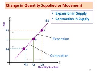
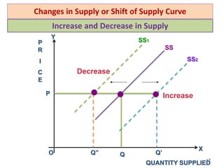
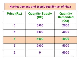
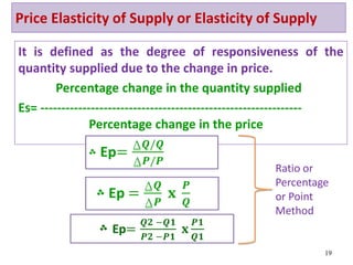
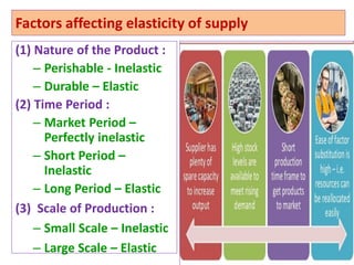
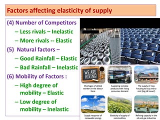
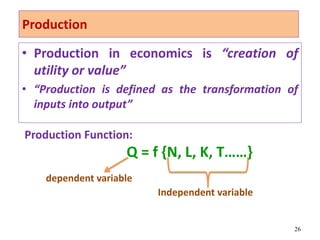
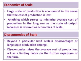
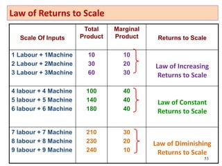
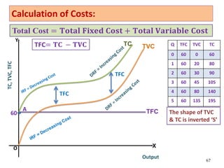
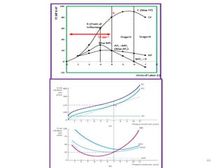
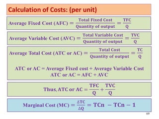
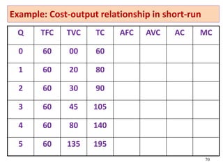
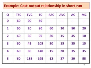
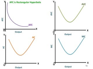
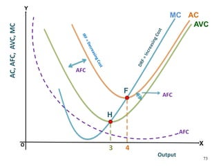
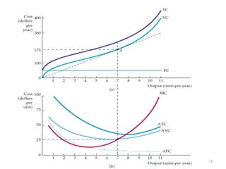
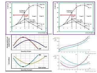
Supply, Production and Cost Analysis
• Supply Analysis: Introduction, Meaning of Supply and
Law of Supply, Exceptions to the Law of Supply, Changes
or Shifts in Supply. Elasticity of supply, Factors
Determining Elasticity of Supply, Practical Importance.
• Market Equilibrium and Changes in Market Equilibrium.
• Production Analysis: Introduction, Meaning of
Production and Production Function,
• Cost of Production: Cost Analysis: Private costs and
Social Costs, Accounting Costs and Economic costs,
Short run and Long Run costs, Economies of scale, Cost-
Output Relationship - Cost Function, Cost-Output
Relationships in the Short Run, and Cost-Output
Relationships in the Long Run.
4/27/2021 Prepared by Dr. Samita Mahapatra
2
The Supply Decision
“THE WILL TO WIN IS IMPORTANT, BUT THE
WILL TO PREPARE IS MORE IMPORTANT”
SUPPLY ANALYSIS
• “Supply is defined as the amount of the commodity
which the seller or producers are able and willing to
offer for sale at a particular price, during a certain
period of time.”
3
Supply Function—
QSx = f { Px, St, Tr, Cp, Fp, Gp…….}
Independent Variable
Dependent Variable
Short – Run Function— QSx = f (Px)
Dependent Variable Independent Variable
Determinants of Supply
1. Price of the Commodity
2. Natural conditions
3. State of Technology
4. Transport conditions
5. Factor prices and their availability
6. Government Policy
7. Number of competitors
4
Law of Supply
• Law of Supply states that, “Other things remaining
the same (Ceterius Paribus) when the price of the
commodity increases the quantity supplied
increases.”
QSx = f {Px}
5
Price of Pizza (Rs.) Quantity Supplied (units) Producer A
500 8
400 7
300 5
200 3
100 0
Market Supply Schedule –Horizontal summation of
individual supply schedule
Price of
Pizza
(Rs.)
QS by
Mr. A
QS by
Mr. B
QS by
Mr. C
Market
Supply
500 8 10 12 30
400 7 9 11 27
300 5 8 10 23
200 3 7 0 10
100 0 6 0 6
6
7
Producer A’s Supply Curve of Pizza
SS
P
P1
Q Q1
Quantity Supplied
Price
O
Y
X
8
Exceptions to the Law of Supply
1. Backward Bending Supply Curve of Labour.
9
X
Y SS
b
c
a
L” L’
L
w”
w’
w
Wage
rate
Number of Laborers
O
Exceptions to the Law of Supply:
2. Land, Rare paintings or
antics
3. Perishable goods
4. Agriculture goods
5. Goods for auction
6. Disposal of stock
10
X
Y
SS
Q
P”
P’
P
P
r
i
c
e
Land, rare paintings,
perishable goods, stock
O
Change in Quantity Supplied or Movement
• Expansion in Supply
• Contraction in Supply
11
Y
X
Price
Quantity Supplied
a
b
c
Q1
Q
Q2
P1
P
P2
Contraction
Expansion
SS
Changes in Supply or Shift of Supply Curve
12
X
Y
P
R
I
C
E
QUANTITY SUPPLIED
SS
SS2
SS1
Q” Q Q’
P
O
Decrease
Increase
Increase and Decrease in Supply
13
“No-Case-on-the –Table” Principle
Market Demand and Supply Equilibrium of Pizza
Price (Rs.) Quantity Supply
(QS)
Quantity
Demanded
(QD)
6 8000 2000
5 6000 3000
4 4000 4000
3 2000 5000
2 0 6000
14
Market or Industry Equilibrium
15
X
Y
Price
Quantity Demanded and Supplied
DD SS
4
4000
E
5
SURPLUS
SS > DD
O
Producers
bid the
price down
Price (Rs.) (QS) (QD)
6 8000 2000
5 6000 3000
4 4000 4000
3 2000 5000
2 0 6000
Demand = Supply
Market or Industry Equilibrium
16
X
Y
Price
Quantity demanded and supplied
DD SS
4
4000
E
O
3
Shortage DD>SS
Consumers bid up
the prices
Price (Rs.) (QS) (QD)
6 8000 2000
5 6000 3000
4 4000 4000
3 2000 5000
2 0 6000
Demand = Supply
Shifts in Market Equilibrium
17
X
Y
Price
Quantity demanded and supplied
SS
DD”
DD’
DD
E”
E
E’
P”
P
P’
Q” Q’
Q
O
18
X
Y
Quantity demanded and supplied
SS
SS’
SS”
E
E’
E”
DD
Q Q’
Q”
P
P”
P’
O
Shifts in Market Equilibrium
Price
Price Elasticity of Supply or Elasticity of Supply
It is defined as the degree of responsiveness of the
quantity supplied due to the change in price.
Percentage change in the quantity supplied
Es= --------------------------------------------------------------
Percentage change in the price
19
Ratio or
Percentage
or Point
Method
Arc Method of Price Elasticity
Prepared by Dr. Samita Mahapatra
es =
Qs2 – Qs1
P
P2 + P1
Qs2 + Qs1
X
Qs
Qs2 + Qs1
2
2
P2 – P1
P2 + P1
es =
4/27/2021
Measurement of Elasticity of Supply
21
Where; P1 = Initial Price
P2 = New Price
Qs1 = Initial quantity supplied
Qs2 = New quantity supplied
Price
Quantity Demanded
Price
Quantity Demanded
Arc
A
B
D
E
C
SS SS
Types of elasticity of Supply
1. Perfectly
elastic (Es=∞)
2. Relatively
elastic (Es>1)
3. Perfectly
inelastic (Es=0)
4. Relatively
inelastic (Es<1)
5. Unitary elastic
(Es=1)
22
X
Y
Price
QUANTITY SUPPLIED
es = ∞
es = 0 es < 1
es = 1
es > 1
O
Factors affecting elasticity of supply
(1) Nature of the Product :
– Perishable - Inelastic
– Durable – Elastic
(2) Time Period :
– Market Period –
Perfectly inelastic
– Short Period –
Inelastic
– Long Period – Elastic
(3) Scale of Production :
– Small Scale – Inelastic
– Large Scale – Elastic 23
Factors affecting elasticity of supply
(4) Number of Competitors
– Less rivals – Inelastic
– More rivals -- Elastic
(5) Natural factors –
– Good Rainfall – Elastic
– Bad Rainfall – Inelastic
(6) Mobility of Factors :
– High degree of
mobility – Elastic
– Low degree of
mobility – Inelastic
24
25
“Minutes Are Worth More Than Money, Spend Them Wisely”
Production Analysis
Production
• Production in economics is “creation of
utility or value”
• “Production is defined as the transformation of
inputs into output”
26
Production Function:
Q = f {N, L, K, T……}
Independent variable
dependent variable
Importance of Production Function
• Gives the idea of Optimum level of output and
employment.
• Tell management the Budget Constraint for increase in
output
• Explains the degree of Substitution and
Complementary of different factors of production
Endeavor to produce an upward shift in production
function.
• Explains the possibility of Disguised unemployment
• Explains the behavior of production function under
different conditions
27
Production Function
28
Long Run Theory
Short Run Theory
Law of Variable Proportions
or Law of Diminishing
Marginal Returns
Law of Returns to Scale
Too Many Cooks Spoil the Broth
The Theory of Law of Variable Proportions
Dr. Samita Mahapatra
Elements:
• Total Product – output produced in Physical units
30
Marginal Product is rate of
change in Total Product
Average Product is Total
Product divided by Quantity of
variable factor (labor)
The Law of Diminishing Returns to Factor or Law
of Variable Proportions
“As equal increments of one input are added; the
inputs of other productive services being held,
constant, beyond a certain point the resulting
increments of product will decrease, i.e., the
marginal product will diminish”. (G. Stigler)
Assumptions:
1. State of technology is constant
2. The quantity of one of the input (Fixed) is constant.
3. The variable Factor is homogeneous.
4. Only physical relationship between the factors are
considered. No monetary value is taken into consideration.
31
32
Land Labor TP AP MP
2 0 0
2 1 20
2 2 50
2 3 90
2 4 120
2 5 140
2 6 150
2 7 150
2 8 130
2 9 100
33
Land Labor TP AP MP
2 0 0 - -
2 1 20 20 20
2 2 50 25 30
2 3 90 30 40
2 4 120 30 30
2 5 140 28 20
2 6 150 25 10
2 7 150 21.5 0
2 8 130 16.25 -20
2 9 100 11.1 -30
Stage- I
Stage- II
Stage- III
34
X
Y
N
H
F
K
TP
AP
MP
o Q
Stage-I: IRF
Stage-II:
DRF
Stage-III: NRF
Point of
Inflexion
Q1 Output
Total
/
Average
/
Marginal
Product
TP’
35
Land Labor TP AP MP
2 0 0 -- --
2 1 15
2 2 20
2 3 20
2 4 76
2 5 15
2 6 15
36
Land Labor TP AP MP
2 0 0 -- --
2 1 15 15 15
2 2 40 20 25
2 3 60 30 20
2 4 76 19 16
2 5 91 18.6 15
2 6 90 15 -1
IRF
DRF
NRF
Application of Law of Variable Proportion :
• Agriculture sector
• Fisheries
• Mining
37
Limitations of Law of Variable Proportions :
• New methods of cultivation
• New Soil
• Insufficient Capital
Practice Multiple Choice Questions
4/27/2021 Prepared by Dr. Samita Mahapatra
1. The point of inflection on the total product curve
corresponds to the level of output where:
a. average product is at a maximum.
b. marginal product is at a maximum.
c. Stage II of production begins.
d. All of these are correct.
39
2. The law of diminishing returns:
a. is reflected in the negatively sloped portion of the marginal
product curve.
b. is the result of specialization and division of labor.
c. applies in both the short run and the long run.
d. All of these are correct.
40
4. By using computers to design and manufacture products,
firms are able to:
a. reduce production costs.
b. reduce the optimal lot size.
c. reduce the time required to introduce new products.
d. All of these are correct
3. Stage II of production begins at the point:
a. where average and marginal product are equal.
b. of inflection of the total product curve.
c. where total product is at a maximum.
d. where marginal product is at a maximum.
41
5. Law of variable proportion explains three stages of
production. In the first stage of production:
a. Both MP and AP rise
b. MP rises
c. AP Falls
d. MP is zero
6. In which stage of production a rational producer likes to
operate in shot-run production ?
a. First Stage
b. Second Stage
c. Third Stage
d. None of these
Dr. Samita Mahapatra
Economies of Scale
• Large scale of production is economical in the sense
that the cost of production is low.
• Anything which serves to minimize average cost of
production in the long run as the scale of output
increases is referred as economies of scale.
44
Diseconomies of Scale
• Beyond a particular limit certain disadvantages of
large scale production emerge.
• Diseconomies raises the average cost of production,
act as a limiting factor on the further expansion of
the firm.
Economies of Scale
45
Internal Economies External Economies
Diseconomies of Scale
Internal Diseconomies External Diseconomies
46
Economies of Scale
Internal Economies
• Technical Economies
• Managerial
Economies
• Financial Economies
• Labour Economies
External Economies
• Economies of
Concentration
• Economies of
Information
• Economies of vertical
Disintegration
• Economies of
By-products
47
Diseconomies of Scale
Internal
Diseconomies
• Technical Problems
• Managerial
Inefficiency
• Financial difficulties
• Unskilled Labor
External
Diseconomies
• Increase in factor prices
• Increase in raw material
prices
• Congestion and
pollution etc
48
Economies of Scope
• It refers to the lowering of costs that a firm often
experience when it produces two or more products
together rather than each alone.
• For example, Printing Machine an be used for
printing magazine, pamphlets, newspaper, visiting
cards, ceremony cards etc.
• Banking sector
49
50
Economies of Scope
Classify the following into Economies and
Diseconomies of scale:
1. Increase in interest rate on loan.
2. Expert consultants.
3. Bureaucracy
4. Political disturbance
5. Fall in the prices of shares in the speculative market.
6. Air Pollution
7. Power cuts.
8. Indefinite transport strike.
9. Ego Clashes among the managers.
10. Expert and efficient laborers. 51
Long Run: Law of Returns to Scale
• Economies of Scale >
Diseconomies of Scale =
Law of Increasing
Returns to Scale
• Economies of Scale =
Diseconomies of Scale =
Law of Constant Returns
to Scale
• Economies of Scale <
Diseconomies of Scale =
Law of Diminishing
Returns to Scale
52
X
Y
Output
O
Input
Constant
Law of Returns to Scale
Scale Of Inputs
Total
Product
Marginal
Product Returns to Scale
1 Labour + 1Machine
2 Labour + 2Machine
3 Labour + 3Machine
10
30
60
10
20
30
Law of Increasing
Returns to Scale
4 labour + 4 Machine
5 labour + 5 Machine
6 labour + 6 Machine
100
140
180
40
40
40
Law of Constant
Returns to Scale
7 labour + 7 Machine
8 labour + 8 Machine
9 labour + 9 Machine
210
230
240
30
20
10
Law of Diminishing
Returns to Scale
53
Practice Multiple Choice Questions
4/27/2021 Prepared by Dr. Samita Mahapatra
55
1. What do economies of scale result in a fall in?
a. Total Cost
b. Sales Revenue
c. Total Profits
d. Average Cost
2. What are diseconomies of scale most likely to be caused by?
a. Increased competition
b. Increased communication as firm grows in size
c. Reduced motivation as a firm grows in size
d. Reduction in average cost
3. What are purchasing economies?
a. When a company buys in bulk and at a discount.
b. An example of spreading fixed costs over a larger level of
output
c. Barriers to communication
d. When the inventory pile up in the company
56
4. The long run is a period of time in which:
a. the firm is able to maximize total profit
b. the firm may want to build a bigger plant, but cannot do so
c. the quantities of all inputs can be varied.
d. economic efficiency is achieved
5. What does spreading fixed costs over a larger level of output
always cause?
a. Economies of scale
b. Diseconomies of scale
c. Growth
d. Competition
57
6. Which of the following explains the short-run production
function ?
a. Law of demand
b. Law of variable proportions
c. Returns to scale
d. Elasticity of demand
7. Long-run production function is related to:
a. Law of Demand
b. Law of Increasing Returns
c. Laws of Returns to Scale
d. Elasticity of Demand
58
“Great Minds Discuss Ideas, Average Minds Discuss
Events, Small Minds Discuss People”
Cost Analysis
Cost:
The term ‘cost’ is most widely used as the ‘money cost’ of
production which relates to the money expenditure of a firm.
The firm incurs following expenditures:
• Wages and salaries paid to the labor.
• Payment incurred on machinery and equipment.
• Payment for materials, power, light, fuel, transportation etc.
• Payments for rent and insurance. 59
Classification of Costs:
60
Private Cost:
While producing a firm has to
pay for raw materials, wages
for workers, it has to pay for
rent of building etc. These are
private costs of the firm.
Social Cost:
Factories emit large about of
smoke from their chimneys into
the atmosphere. Which is not
calculated by the firm. But the
cost of community increases in
buying better quality washing
powder, medical bills etc. These
are social costs.
Accounting Cost:
Cost paid out of pocket. It is
explicit cost. Measured strictly
in monetary terms.
Accounting cost = Explicit Cost
61
Classification of Costs:
Economic Cost :
Cost to a firm of utilizing
economic resources in
production, including
opportunity cost. It includes
implicit cost.
EC = Explicit + Implicit Cost
Opportunity Cost:
• The next best alternative
foregone when an alternative
is selected.
• Example; If you were not
attending the college, you
could have earned Rs. 20,000
a year. So your opportunity
cost of attending a college is
Rs. 20,000 per year.
62
Classification of Costs:
63
64
Fixed costs (Prime Costs):
Cost which remains fixed irrespective of the level of output
produced. They remain constant in the short run can change only
in the long run. For example, plant, machinery, building etc. It is
time related. 65
Classification of Costs:
Variable cost (Supplementary Costs):
Cost that varies/changes in relation to volume of production. The
cost that changes with the level of output in the short run as
well as in the long run. For example, labour, raw material, fuel
etc 66
Classification of Costs:
67
Calculation of Costs:
TFC
O
Output
X
Y
A
Q TFC TVC TC
0 60 0 60
1 60 20 80
2 60 30 90
3 60 45 105
4 60 80 140
5 60 135 195
TVC
TC
60
TFC
TFC
TC,
TVC,
TFC
The shape of TVC
& TC is inverted ‘S’
68
69
Calculation of Costs: (per unit)
Example: Cost-output relationship in short-run
Q TFC TVC TC AFC AVC AC MC
0 60 00 60
1 60 20 80
2 60 30 90
3 60 45 105
4 60 80 140
5 60 135 195
70
Q TFC TVC TC AFC AVC AC MC
0 60 00 60 -- -- -- --
1 60 20 80 60 20 80 20
2 60 30 90 30 15 45 10
3 60 45 105 20 15 35 15
4 60 80 140 15 20 35 35
5 60 135 195 12 27 39 55
71
Example: Cost-output relationship in short-run
72
AFC
O
Output
X
Y
AFC AFC is Rectangular Hyperbola Y
X
O
AVC
Output
AVC
Y
X
O
AC
Output
AC
Y
X
O
MC
Output
MC
73
AVC
O
Output
X
Y
AC,
AFC,
AVC,
MC AC
MC
F
H
AFC
AFC
3 4
AFC
74
75
Example: Construct the cost schedules.
Q MC TFC TVC TC AFC AVC AC
0 --
1 30
2 25
3 20
4 30
5 50 11
6 70
7 90
Example: construct the cost schedule and explain the cost-output
relationships in short -run
Q TFC TVC TC AFC AVC AC MC
0 250
1 100
2 210
3 220
4 510
5 60
6 100
7 60
8 590
9 90
77
Example: Calculate the missing numbers and explain the cost-
output relationship
Q TFC TVC TC MC AFC AVC AC
1 100 50
2 30
3 40
4 270
5 70
79
SRAC3
SRAC1
SRAC2 SRAC4
SRAC5
Output
Costs
O
LRAC
F
H
K
L
J
Q1 Q2 Q Q3
Optimum level
of output
X
Y
500 800 1500
Constant
returns to Scale
LRAC Curve is called Planning Curve or Envelope Curve
80
SAC1 SAC2 SAC3 SAC4
Q AC($) Q AC($) Q AC($) Q AC($)
1 20.00 3 16.00 5 13.00 9 12.00
2 17.00 4 13.00 6 11.50 10 11.50
3 15.50 5 12.20 7 10.50 11 11.70
4 15.00 6 12.00 8 10.00 12 12.00
5 16.00 7 13.00 9 10.50 13 13.50
6 18.00 8 15.00 10 11.00
11 12.00
Example: Plot the table in a graph and find the optimum output
81
SAC1 SAC2 SAC3 SAC4
Q AC($) Q AC($) Q AC($) Q AC($)
1 20.00 3 16.00 5 13.00 9 12.00
2 17.00 4 13.00 6 11.50 10 11.50
3 15.50 5 12.20 7 10.50 11 11.70
4 15.00 6 12.00 8 10.00 12 12.00
5 16.00 7 13.00 9 10.50 13 13.50
6 18.00 8 15.00 10 11.00
11 12.00
Example: Plot the table in a graph and find the optimum output
82
Practice Multiple Choice Questions
4/27/2021 Prepared by Dr. Samita Mahapatra
84
1. Look carefully at the table
which represents a firm's short-
run total cost schedule. When
output goes up from four to five
shirts the marginal cost is:
a. 25
b. 30
c. 4
d. 20
Output Total Cost (Rs)
3 25
4 55
5 75
6 79
2. Which one of the following statements is false?
a. Marginal cost is the increase in total cost resulting from a
unit increase in output.
b. Average fixed cost plus average variable cost equals average
total cost.
c. Marginal cost depends on the amount of labor hired.
d. Total cost equals total fixed cost plus total average cost.
85
3. Which one of the following statements is false? (refer the figure)
a. Curve B comes closer to curve C as output increases
because of a decrease in average fixed costs.
b. The vertical gap between curves B and C is equal to
average fixed cost.
c. The vertical gap between curves B and C is equal to
average variable cost.
d. Average fixed cost decreases with output.
86
4. In the figure the average
variable cost curve is
represented by the curve
labelled:
a. B
b. D
c. A
d. C
5. The marginal cost (MC) curve intersects the:
a. ATC, AVC and AFC curves at their minimum points
b. ATC curve at its maximizing point
c. ATC and AVC curves at their minimum points
d. AVC and AFC curves at their minimum points
87
9. Opportunity cost means:
a. The accounting cost minus the marginal benefit.
b. The highest-valued alternative forgone.
c. The monetary costs of an activity.
d. The accounting cost minus the marginal cost.
10. Variable costs are:
a. sunk costs.
b. multiplied by fixed costs.
c. costs that change with the level of production.
d. defined as the change in total cost resulting from the
production of an additional unit of output.
88
6. Cost functions are derived from:
a. Demand functions
b. Supply functions
c. Production functions
d. Revenue functions
7. Which cost are recorded in books of accounts?
a. Real cost
b. Social cost
c. Implicit cost
d. Explicit cost
8. Which cost is more useful for decision making?
a. Real cost
b. Social cost
c. Opportunity cost
d. Explicit cost

Supply, Production and Cost Analysis

  • 1.
    Supply, Production andCost Analysis • Supply Analysis: Introduction, Meaning of Supply and Law of Supply, Exceptions to the Law of Supply, Changes or Shifts in Supply. Elasticity of supply, Factors Determining Elasticity of Supply, Practical Importance. • Market Equilibrium and Changes in Market Equilibrium. • Production Analysis: Introduction, Meaning of Production and Production Function, • Cost of Production: Cost Analysis: Private costs and Social Costs, Accounting Costs and Economic costs, Short run and Long Run costs, Economies of scale, Cost- Output Relationship - Cost Function, Cost-Output Relationships in the Short Run, and Cost-Output Relationships in the Long Run. 4/27/2021 Prepared by Dr. Samita Mahapatra
  • 2.
    2 The Supply Decision “THEWILL TO WIN IS IMPORTANT, BUT THE WILL TO PREPARE IS MORE IMPORTANT”
  • 3.
    SUPPLY ANALYSIS • “Supplyis defined as the amount of the commodity which the seller or producers are able and willing to offer for sale at a particular price, during a certain period of time.” 3 Supply Function— QSx = f { Px, St, Tr, Cp, Fp, Gp…….} Independent Variable Dependent Variable Short – Run Function— QSx = f (Px) Dependent Variable Independent Variable
  • 4.
    Determinants of Supply 1.Price of the Commodity 2. Natural conditions 3. State of Technology 4. Transport conditions 5. Factor prices and their availability 6. Government Policy 7. Number of competitors 4
  • 5.
    Law of Supply •Law of Supply states that, “Other things remaining the same (Ceterius Paribus) when the price of the commodity increases the quantity supplied increases.” QSx = f {Px} 5 Price of Pizza (Rs.) Quantity Supplied (units) Producer A 500 8 400 7 300 5 200 3 100 0
  • 6.
    Market Supply Schedule–Horizontal summation of individual supply schedule Price of Pizza (Rs.) QS by Mr. A QS by Mr. B QS by Mr. C Market Supply 500 8 10 12 30 400 7 9 11 27 300 5 8 10 23 200 3 7 0 10 100 0 6 0 6 6
  • 7.
    7 Producer A’s SupplyCurve of Pizza SS P P1 Q Q1 Quantity Supplied Price O Y X
  • 8.
  • 9.
    Exceptions to theLaw of Supply 1. Backward Bending Supply Curve of Labour. 9 X Y SS b c a L” L’ L w” w’ w Wage rate Number of Laborers O
  • 10.
    Exceptions to theLaw of Supply: 2. Land, Rare paintings or antics 3. Perishable goods 4. Agriculture goods 5. Goods for auction 6. Disposal of stock 10 X Y SS Q P” P’ P P r i c e Land, rare paintings, perishable goods, stock O
  • 11.
    Change in QuantitySupplied or Movement • Expansion in Supply • Contraction in Supply 11 Y X Price Quantity Supplied a b c Q1 Q Q2 P1 P P2 Contraction Expansion SS
  • 12.
    Changes in Supplyor Shift of Supply Curve 12 X Y P R I C E QUANTITY SUPPLIED SS SS2 SS1 Q” Q Q’ P O Decrease Increase Increase and Decrease in Supply
  • 13.
  • 14.
    Market Demand andSupply Equilibrium of Pizza Price (Rs.) Quantity Supply (QS) Quantity Demanded (QD) 6 8000 2000 5 6000 3000 4 4000 4000 3 2000 5000 2 0 6000 14
  • 15.
    Market or IndustryEquilibrium 15 X Y Price Quantity Demanded and Supplied DD SS 4 4000 E 5 SURPLUS SS > DD O Producers bid the price down Price (Rs.) (QS) (QD) 6 8000 2000 5 6000 3000 4 4000 4000 3 2000 5000 2 0 6000 Demand = Supply
  • 16.
    Market or IndustryEquilibrium 16 X Y Price Quantity demanded and supplied DD SS 4 4000 E O 3 Shortage DD>SS Consumers bid up the prices Price (Rs.) (QS) (QD) 6 8000 2000 5 6000 3000 4 4000 4000 3 2000 5000 2 0 6000 Demand = Supply
  • 17.
    Shifts in MarketEquilibrium 17 X Y Price Quantity demanded and supplied SS DD” DD’ DD E” E E’ P” P P’ Q” Q’ Q O
  • 18.
    18 X Y Quantity demanded andsupplied SS SS’ SS” E E’ E” DD Q Q’ Q” P P” P’ O Shifts in Market Equilibrium Price
  • 19.
    Price Elasticity ofSupply or Elasticity of Supply It is defined as the degree of responsiveness of the quantity supplied due to the change in price. Percentage change in the quantity supplied Es= -------------------------------------------------------------- Percentage change in the price 19 Ratio or Percentage or Point Method
  • 20.
    Arc Method ofPrice Elasticity Prepared by Dr. Samita Mahapatra es = Qs2 – Qs1 P P2 + P1 Qs2 + Qs1 X Qs Qs2 + Qs1 2 2 P2 – P1 P2 + P1 es = 4/27/2021
  • 21.
    Measurement of Elasticityof Supply 21 Where; P1 = Initial Price P2 = New Price Qs1 = Initial quantity supplied Qs2 = New quantity supplied Price Quantity Demanded Price Quantity Demanded Arc A B D E C SS SS
  • 22.
    Types of elasticityof Supply 1. Perfectly elastic (Es=∞) 2. Relatively elastic (Es>1) 3. Perfectly inelastic (Es=0) 4. Relatively inelastic (Es<1) 5. Unitary elastic (Es=1) 22 X Y Price QUANTITY SUPPLIED es = ∞ es = 0 es < 1 es = 1 es > 1 O
  • 23.
    Factors affecting elasticityof supply (1) Nature of the Product : – Perishable - Inelastic – Durable – Elastic (2) Time Period : – Market Period – Perfectly inelastic – Short Period – Inelastic – Long Period – Elastic (3) Scale of Production : – Small Scale – Inelastic – Large Scale – Elastic 23
  • 24.
    Factors affecting elasticityof supply (4) Number of Competitors – Less rivals – Inelastic – More rivals -- Elastic (5) Natural factors – – Good Rainfall – Elastic – Bad Rainfall – Inelastic (6) Mobility of Factors : – High degree of mobility – Elastic – Low degree of mobility – Inelastic 24
  • 25.
    25 “Minutes Are WorthMore Than Money, Spend Them Wisely” Production Analysis
  • 26.
    Production • Production ineconomics is “creation of utility or value” • “Production is defined as the transformation of inputs into output” 26 Production Function: Q = f {N, L, K, T……} Independent variable dependent variable
  • 27.
    Importance of ProductionFunction • Gives the idea of Optimum level of output and employment. • Tell management the Budget Constraint for increase in output • Explains the degree of Substitution and Complementary of different factors of production Endeavor to produce an upward shift in production function. • Explains the possibility of Disguised unemployment • Explains the behavior of production function under different conditions 27
  • 28.
    Production Function 28 Long RunTheory Short Run Theory Law of Variable Proportions or Law of Diminishing Marginal Returns Law of Returns to Scale
  • 29.
    Too Many CooksSpoil the Broth The Theory of Law of Variable Proportions Dr. Samita Mahapatra
  • 30.
    Elements: • Total Product– output produced in Physical units 30 Marginal Product is rate of change in Total Product Average Product is Total Product divided by Quantity of variable factor (labor)
  • 31.
    The Law ofDiminishing Returns to Factor or Law of Variable Proportions “As equal increments of one input are added; the inputs of other productive services being held, constant, beyond a certain point the resulting increments of product will decrease, i.e., the marginal product will diminish”. (G. Stigler) Assumptions: 1. State of technology is constant 2. The quantity of one of the input (Fixed) is constant. 3. The variable Factor is homogeneous. 4. Only physical relationship between the factors are considered. No monetary value is taken into consideration. 31
  • 32.
    32 Land Labor TPAP MP 2 0 0 2 1 20 2 2 50 2 3 90 2 4 120 2 5 140 2 6 150 2 7 150 2 8 130 2 9 100
  • 33.
    33 Land Labor TPAP MP 2 0 0 - - 2 1 20 20 20 2 2 50 25 30 2 3 90 30 40 2 4 120 30 30 2 5 140 28 20 2 6 150 25 10 2 7 150 21.5 0 2 8 130 16.25 -20 2 9 100 11.1 -30 Stage- I Stage- II Stage- III
  • 34.
    34 X Y N H F K TP AP MP o Q Stage-I: IRF Stage-II: DRF Stage-III:NRF Point of Inflexion Q1 Output Total / Average / Marginal Product TP’
  • 35.
    35 Land Labor TPAP MP 2 0 0 -- -- 2 1 15 2 2 20 2 3 20 2 4 76 2 5 15 2 6 15
  • 36.
    36 Land Labor TPAP MP 2 0 0 -- -- 2 1 15 15 15 2 2 40 20 25 2 3 60 30 20 2 4 76 19 16 2 5 91 18.6 15 2 6 90 15 -1 IRF DRF NRF
  • 37.
    Application of Lawof Variable Proportion : • Agriculture sector • Fisheries • Mining 37 Limitations of Law of Variable Proportions : • New methods of cultivation • New Soil • Insufficient Capital
  • 38.
    Practice Multiple ChoiceQuestions 4/27/2021 Prepared by Dr. Samita Mahapatra
  • 39.
    1. The pointof inflection on the total product curve corresponds to the level of output where: a. average product is at a maximum. b. marginal product is at a maximum. c. Stage II of production begins. d. All of these are correct. 39 2. The law of diminishing returns: a. is reflected in the negatively sloped portion of the marginal product curve. b. is the result of specialization and division of labor. c. applies in both the short run and the long run. d. All of these are correct.
  • 40.
    40 4. By usingcomputers to design and manufacture products, firms are able to: a. reduce production costs. b. reduce the optimal lot size. c. reduce the time required to introduce new products. d. All of these are correct 3. Stage II of production begins at the point: a. where average and marginal product are equal. b. of inflection of the total product curve. c. where total product is at a maximum. d. where marginal product is at a maximum.
  • 41.
    41 5. Law ofvariable proportion explains three stages of production. In the first stage of production: a. Both MP and AP rise b. MP rises c. AP Falls d. MP is zero 6. In which stage of production a rational producer likes to operate in shot-run production ? a. First Stage b. Second Stage c. Third Stage d. None of these
  • 43.
  • 44.
    Economies of Scale •Large scale of production is economical in the sense that the cost of production is low. • Anything which serves to minimize average cost of production in the long run as the scale of output increases is referred as economies of scale. 44 Diseconomies of Scale • Beyond a particular limit certain disadvantages of large scale production emerge. • Diseconomies raises the average cost of production, act as a limiting factor on the further expansion of the firm.
  • 45.
    Economies of Scale 45 InternalEconomies External Economies Diseconomies of Scale Internal Diseconomies External Diseconomies
  • 46.
  • 47.
    Economies of Scale InternalEconomies • Technical Economies • Managerial Economies • Financial Economies • Labour Economies External Economies • Economies of Concentration • Economies of Information • Economies of vertical Disintegration • Economies of By-products 47
  • 48.
    Diseconomies of Scale Internal Diseconomies •Technical Problems • Managerial Inefficiency • Financial difficulties • Unskilled Labor External Diseconomies • Increase in factor prices • Increase in raw material prices • Congestion and pollution etc 48
  • 49.
    Economies of Scope •It refers to the lowering of costs that a firm often experience when it produces two or more products together rather than each alone. • For example, Printing Machine an be used for printing magazine, pamphlets, newspaper, visiting cards, ceremony cards etc. • Banking sector 49
  • 50.
  • 51.
    Classify the followinginto Economies and Diseconomies of scale: 1. Increase in interest rate on loan. 2. Expert consultants. 3. Bureaucracy 4. Political disturbance 5. Fall in the prices of shares in the speculative market. 6. Air Pollution 7. Power cuts. 8. Indefinite transport strike. 9. Ego Clashes among the managers. 10. Expert and efficient laborers. 51
  • 52.
    Long Run: Lawof Returns to Scale • Economies of Scale > Diseconomies of Scale = Law of Increasing Returns to Scale • Economies of Scale = Diseconomies of Scale = Law of Constant Returns to Scale • Economies of Scale < Diseconomies of Scale = Law of Diminishing Returns to Scale 52 X Y Output O Input Constant
  • 53.
    Law of Returnsto Scale Scale Of Inputs Total Product Marginal Product Returns to Scale 1 Labour + 1Machine 2 Labour + 2Machine 3 Labour + 3Machine 10 30 60 10 20 30 Law of Increasing Returns to Scale 4 labour + 4 Machine 5 labour + 5 Machine 6 labour + 6 Machine 100 140 180 40 40 40 Law of Constant Returns to Scale 7 labour + 7 Machine 8 labour + 8 Machine 9 labour + 9 Machine 210 230 240 30 20 10 Law of Diminishing Returns to Scale 53
  • 54.
    Practice Multiple ChoiceQuestions 4/27/2021 Prepared by Dr. Samita Mahapatra
  • 55.
    55 1. What doeconomies of scale result in a fall in? a. Total Cost b. Sales Revenue c. Total Profits d. Average Cost 2. What are diseconomies of scale most likely to be caused by? a. Increased competition b. Increased communication as firm grows in size c. Reduced motivation as a firm grows in size d. Reduction in average cost 3. What are purchasing economies? a. When a company buys in bulk and at a discount. b. An example of spreading fixed costs over a larger level of output c. Barriers to communication d. When the inventory pile up in the company
  • 56.
    56 4. The longrun is a period of time in which: a. the firm is able to maximize total profit b. the firm may want to build a bigger plant, but cannot do so c. the quantities of all inputs can be varied. d. economic efficiency is achieved 5. What does spreading fixed costs over a larger level of output always cause? a. Economies of scale b. Diseconomies of scale c. Growth d. Competition
  • 57.
    57 6. Which ofthe following explains the short-run production function ? a. Law of demand b. Law of variable proportions c. Returns to scale d. Elasticity of demand 7. Long-run production function is related to: a. Law of Demand b. Law of Increasing Returns c. Laws of Returns to Scale d. Elasticity of Demand
  • 58.
    58 “Great Minds DiscussIdeas, Average Minds Discuss Events, Small Minds Discuss People” Cost Analysis
  • 59.
    Cost: The term ‘cost’is most widely used as the ‘money cost’ of production which relates to the money expenditure of a firm. The firm incurs following expenditures: • Wages and salaries paid to the labor. • Payment incurred on machinery and equipment. • Payment for materials, power, light, fuel, transportation etc. • Payments for rent and insurance. 59
  • 60.
    Classification of Costs: 60 PrivateCost: While producing a firm has to pay for raw materials, wages for workers, it has to pay for rent of building etc. These are private costs of the firm. Social Cost: Factories emit large about of smoke from their chimneys into the atmosphere. Which is not calculated by the firm. But the cost of community increases in buying better quality washing powder, medical bills etc. These are social costs.
  • 61.
    Accounting Cost: Cost paidout of pocket. It is explicit cost. Measured strictly in monetary terms. Accounting cost = Explicit Cost 61 Classification of Costs: Economic Cost : Cost to a firm of utilizing economic resources in production, including opportunity cost. It includes implicit cost. EC = Explicit + Implicit Cost
  • 62.
    Opportunity Cost: • Thenext best alternative foregone when an alternative is selected. • Example; If you were not attending the college, you could have earned Rs. 20,000 a year. So your opportunity cost of attending a college is Rs. 20,000 per year. 62 Classification of Costs:
  • 63.
  • 64.
  • 65.
    Fixed costs (PrimeCosts): Cost which remains fixed irrespective of the level of output produced. They remain constant in the short run can change only in the long run. For example, plant, machinery, building etc. It is time related. 65 Classification of Costs:
  • 66.
    Variable cost (SupplementaryCosts): Cost that varies/changes in relation to volume of production. The cost that changes with the level of output in the short run as well as in the long run. For example, labour, raw material, fuel etc 66 Classification of Costs:
  • 67.
    67 Calculation of Costs: TFC O Output X Y A QTFC TVC TC 0 60 0 60 1 60 20 80 2 60 30 90 3 60 45 105 4 60 80 140 5 60 135 195 TVC TC 60 TFC TFC TC, TVC, TFC The shape of TVC & TC is inverted ‘S’
  • 68.
  • 69.
  • 70.
    Example: Cost-output relationshipin short-run Q TFC TVC TC AFC AVC AC MC 0 60 00 60 1 60 20 80 2 60 30 90 3 60 45 105 4 60 80 140 5 60 135 195 70
  • 71.
    Q TFC TVCTC AFC AVC AC MC 0 60 00 60 -- -- -- -- 1 60 20 80 60 20 80 20 2 60 30 90 30 15 45 10 3 60 45 105 20 15 35 15 4 60 80 140 15 20 35 35 5 60 135 195 12 27 39 55 71 Example: Cost-output relationship in short-run
  • 72.
    72 AFC O Output X Y AFC AFC isRectangular Hyperbola Y X O AVC Output AVC Y X O AC Output AC Y X O MC Output MC
  • 73.
  • 74.
  • 75.
  • 76.
    Example: Construct thecost schedules. Q MC TFC TVC TC AFC AVC AC 0 -- 1 30 2 25 3 20 4 30 5 50 11 6 70 7 90
  • 77.
    Example: construct thecost schedule and explain the cost-output relationships in short -run Q TFC TVC TC AFC AVC AC MC 0 250 1 100 2 210 3 220 4 510 5 60 6 100 7 60 8 590 9 90 77
  • 78.
    Example: Calculate themissing numbers and explain the cost- output relationship Q TFC TVC TC MC AFC AVC AC 1 100 50 2 30 3 40 4 270 5 70
  • 79.
    79 SRAC3 SRAC1 SRAC2 SRAC4 SRAC5 Output Costs O LRAC F H K L J Q1 Q2Q Q3 Optimum level of output X Y 500 800 1500 Constant returns to Scale LRAC Curve is called Planning Curve or Envelope Curve
  • 80.
    80 SAC1 SAC2 SAC3SAC4 Q AC($) Q AC($) Q AC($) Q AC($) 1 20.00 3 16.00 5 13.00 9 12.00 2 17.00 4 13.00 6 11.50 10 11.50 3 15.50 5 12.20 7 10.50 11 11.70 4 15.00 6 12.00 8 10.00 12 12.00 5 16.00 7 13.00 9 10.50 13 13.50 6 18.00 8 15.00 10 11.00 11 12.00 Example: Plot the table in a graph and find the optimum output
  • 81.
    81 SAC1 SAC2 SAC3SAC4 Q AC($) Q AC($) Q AC($) Q AC($) 1 20.00 3 16.00 5 13.00 9 12.00 2 17.00 4 13.00 6 11.50 10 11.50 3 15.50 5 12.20 7 10.50 11 11.70 4 15.00 6 12.00 8 10.00 12 12.00 5 16.00 7 13.00 9 10.50 13 13.50 6 18.00 8 15.00 10 11.00 11 12.00 Example: Plot the table in a graph and find the optimum output
  • 82.
  • 83.
    Practice Multiple ChoiceQuestions 4/27/2021 Prepared by Dr. Samita Mahapatra
  • 84.
    84 1. Look carefullyat the table which represents a firm's short- run total cost schedule. When output goes up from four to five shirts the marginal cost is: a. 25 b. 30 c. 4 d. 20 Output Total Cost (Rs) 3 25 4 55 5 75 6 79 2. Which one of the following statements is false? a. Marginal cost is the increase in total cost resulting from a unit increase in output. b. Average fixed cost plus average variable cost equals average total cost. c. Marginal cost depends on the amount of labor hired. d. Total cost equals total fixed cost plus total average cost.
  • 85.
    85 3. Which oneof the following statements is false? (refer the figure) a. Curve B comes closer to curve C as output increases because of a decrease in average fixed costs. b. The vertical gap between curves B and C is equal to average fixed cost. c. The vertical gap between curves B and C is equal to average variable cost. d. Average fixed cost decreases with output.
  • 86.
    86 4. In thefigure the average variable cost curve is represented by the curve labelled: a. B b. D c. A d. C 5. The marginal cost (MC) curve intersects the: a. ATC, AVC and AFC curves at their minimum points b. ATC curve at its maximizing point c. ATC and AVC curves at their minimum points d. AVC and AFC curves at their minimum points
  • 87.
    87 9. Opportunity costmeans: a. The accounting cost minus the marginal benefit. b. The highest-valued alternative forgone. c. The monetary costs of an activity. d. The accounting cost minus the marginal cost. 10. Variable costs are: a. sunk costs. b. multiplied by fixed costs. c. costs that change with the level of production. d. defined as the change in total cost resulting from the production of an additional unit of output.
  • 88.
    88 6. Cost functionsare derived from: a. Demand functions b. Supply functions c. Production functions d. Revenue functions 7. Which cost are recorded in books of accounts? a. Real cost b. Social cost c. Implicit cost d. Explicit cost 8. Which cost is more useful for decision making? a. Real cost b. Social cost c. Opportunity cost d. Explicit cost